Discrete time models

Derivatives 1, professor Alexei Zhdanov

Fall 2010

Handout 2

This handout has benefited from the materials provided by Tony Berrada.

1 / 22

Binomial Model

Definition [Arbitrage]. An arbitrage strategy is a strategy whichrequires no (positive) initial investment, never yields a negativeterminal value and has a strictly positive expected terminal value

2 / 22

One Period Model

The binomial market consists initially of two assets

A risky stockA risk-free bond

We call the beginning of the period time 0 and the end of theperiod time 1

The price of the stock at time 0 is S0

The price of the bond at time zero is B0

The price of the stock at time 1 is a random variableS1 ∈ {Su, Sd}The price of the bond at time 1 is a non random variable B1

3 / 22

One Period Model

Define the risk free interest rate as 1 + r = B1B0

The risky return on stock is u = SuS0

or d = SdS0

Let us call p the probability of an ”up” move and 1− p theprobability of a ”down” moveNormalize the model by setting B0 = 1

4 / 22

Replication

Consider a European call option written on the underlyingasset S with exercise price K and maturity at date 1

The payoff of the option is

cu = (Su −K)+ or cd = (Sd −K)+

The price of the option at time 0 is c0

How can we find it?

5 / 22

Replication

Consider a portfolio V consisting of ∆ shares of the stock andβ shares of the bond

β shares of the bond correspond to an investment of β dollarsat the risk-free rate

The value of the portfolio at time 0 is

V0 = ∆× S0 + β

The value of the portfolio at time 1 is given by

Vu = ∆× Su + β(1 + r) and Vd = ∆× Sd + β(1 + r)

We can construct a portfolio consisting of the stock and thebond such that its value at time 1 is always equal to thepayoff of the option

6 / 22

Replication

We call this portfolio a ”replicating portfolio”

(∆∗, β∗) must be such that

cu = (Su −K)+ = ∆∗ × Su + β∗(1 + r)

cd = (Sd −K)+ = ∆∗ × Sd + β∗(1 + r)

The value of this portfolio today must be equal to the price ofthe call to prevent arbitrage:

c0 = ∆∗ × S0 + β∗

Solving this system of equations yields

∆∗ =cu − cdSu − Sd

β∗ =Sucd − Sdcu

(Su − Sd)(1 + r)

7 / 22

Replication

It follows that the price of the European Call option at time 0is given by

c0 =cu − cdSu − Sd

S0 +Sucd − Sdcu

(Su − Sd)(1 + r)

We can generalize this result to any derivative with payoff(Du, Dd)

D0 =Du −Dd

Su − SdS0 +

SuDd − SdDu

(Su − Sd)(1 + r)

8 / 22

Example

r = 2.5%, S0 = 100, Su = S0u = 125, Sd = S0d = 80,K = 102.5

What is the price of the call option?

What is the price of the put option?

What if the price of the call was $5, $15?

9 / 22

Risk-neutral Valuation

Did we ever use the probability of an ”up” move, p?

What if investors are risk-neutral?

In the risk-neutral world all assets earn the same rate of return- r

Then the ”risk-neutral” probability q :

q =(1 + r)− du− d

and the price of a derivative

D0 =1

1 + r[qDu + (1− q)Dd]

note that it is identical to our no-arbitrage formula

10 / 22

Risk-neutral Valuation

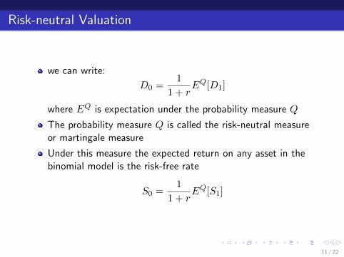
we can write:

D0 =1

1 + rEQ[D1]

where EQ is expectation under the probability measure Q

The probability measure Q is called the risk-neutral measureor martingale measure

Under this measure the expected return on any asset in thebinomial model is the risk-free rate

S0 =1

1 + rEQ[S1]

11 / 22

Multi-period model

We extend the binomial setting to a finer grid

The concepts developed in the one-period model still hold

We still use two assets, the stock and the bond

The bond yields a risk free return of (1 + r) per period

The evolution of the stock price is described by the followingtree

12 / 22

Multi-period model

We will still want to construct a portfolio whose payoffreplicates the payoff of the option at the terminal date

A portfolio starting at time zero with (∆0, β0) can berearranged at any later point in time

We focus our attention on portfolios satisfying the followingcondition

(∆t+1 −∆t)St+1 + (βt+1 − βt)Bt+1 = 0

13 / 22

Multi-period model

We call this portfolio self-financing, as after time 0 they donot require any further cash flow

Self-financing in this case means

∆0Su + β0B1 = ∆uSu + βuB1

∆0Sd + β0B1 = ∆dSd + βdB1

This set of conditions imply

(∆u −∆0)Su + (βu − β0)B1 = 0

(∆d −∆0)Sd + (βd − β0)B1 = 0

We consider a European derivative with maturity at date 2

The payoff is given by some functionD2(S2) ∈ {Duu, Dud, Ddd}

14 / 22

Multi-period model

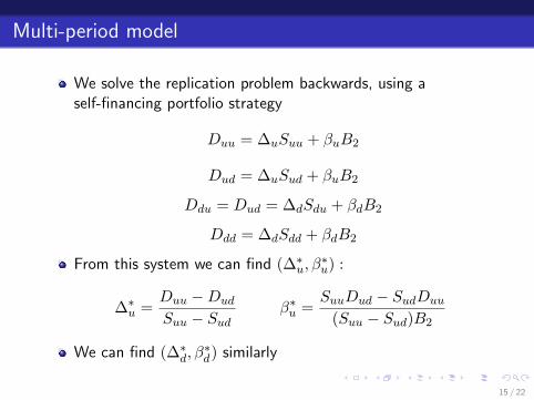
We solve the replication problem backwards, using aself-financing portfolio strategy

Duu = ∆uSuu + βuB2

Dud = ∆uSud + βuB2

Ddu = Dud = ∆dSdu + βdB2

Ddd = ∆dSdd + βdB2

From this system we can find (∆∗u, β

∗u) :

∆∗u =

Duu −Dud

Suu − Sudβ∗u =

SuuDud − SudDuu

(Suu − Sud)B2

We can find (∆∗d, β

∗d) similarly

15 / 22

Multi-period model

Obtaining the price of the derivative at time 0 is similar to theone period problem of replicating a derivative with payoffgiven by

Du = V ∗u = ∆∗

uSu + β∗uB1

Dd = V ∗d = ∆∗

dSd + β∗dB1

Then

∆∗0 =

V ∗u − V ∗

d

Suu − Sudβ∗0 =

SuV∗d − SdV ∗

u

(Su − Sd)B1

And we have solved the replication problem for any Europeanderivative

D0 = V ∗0 = ∆∗

0S0 + β∗0

Note that it is important that our strategy be self-financing.Why?

16 / 22

Example

r = 2.5%, S0 = 100, u = 1.25, d = 0.8, K = 100, T = 2

What is the price of the call option?

What if the price of the call was $20?

17 / 22

Risk-neutral valuation

We can also interpret the pricing equation as expectation

Du =1

1 + r[qDuu + (1− q)Dud] =

1

1 + rEQ[D2|S1 = Su]

Dd =1

1 + r[qDdu + (1− q)Ddd] =

1

1 + rEQ[D2|S1 = Sd]

18 / 22

Risk-neutral valuation

Then

D0 = V ∗0 =

1

1 + r[qDu + (1− q)Dd] =

1

(1 + r)2[q2Duu + (1− q)2Ddd + 2q(1− q)Dud] =

1

(1 + r)2EQ[D2]

The price of a derivative security is the expected value of thepayoff under the risk neutral measure discounted at the riskfree rate

19 / 22

Hedging

Let us go back to the one period model

Consider the problem of the seller of the call option

The seller wants to hedge his short position in the call byholding an adequate quantity of the underlying stock

If this is possible, we will have another way to determine theprice of the option

The perfectly hedged portfolio must have a return equal tothe risk-free rate

A perfect hedge ∆H requires

∆HSu − cu = ∆HSd − cd

20 / 22

Hedging

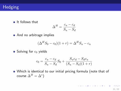
It follows that

∆H =cu − cdSu − Sd

And no arbitrage implies

(∆HS0 − c0)(1 + r) = ∆HSu − cu

Solving for c0 yields

c0 =cu − cdSu − Sd

S0 +Sucd − Sdcu

(Su − Sd)(1 + r)

Which is identical to our initial pricing formula (note that ofcourse ∆H = ∆∗)

21 / 22

Hedging

The ∆ of an option is thus the amount require to hedge ashort position in that option

In a dynamic model, ∆ must be readjusted whenever theunderlying stock price moves

In our multi-period binomial model, the seller adjusts thehedge at any node

22 / 22