DERIVATION OF A NON-LINEAR MODEL EQUATION FOR WAVE PROPAGATION IN BUBBLY LIQUIDS* Domenico Fusco** Francesco Oliveri***

MECCANICA

24 (1989), 15-25

SOMMARIO. Mgdiante l'uso di uno schema asintotico

viene dedotta una equazione differenziale alle derivate parziati del quarto ordine, atta a deserivere l'evoluzione

eli un' onda non lineare propagantesi con la velocitd del suono

in un liquido con bolle. Tale equazione in particolare pre-

scnta detle non tinearita anche helle derivate di ordine pi~

elevato. Infine vengono discussi alcuni risultati numerici

co/messi con la ricerca di soluzion/ del tipo onda stazionaria

e con la relazione di dispersione.

SUMMARY. Through the use o f an asymptotic approach,

it is deduced a fourth order partial differential equation

governing the e~olution o f nonlinear (sound) wave propaga-

tion in bubbly liquids. Remarkably it involves also higher

order nonlinear terms�9 Some results concerning the steady-

state solution as well as the dispersion relation are obtained.

1. INTRODUCI'tON AND GENERAL REMARKS

Great aRention has been paid to the theoretical and

experimental investigation of liquids containing gas bubbles. Actually such a topic has proved to be relevant in several physical and industrial applications such as cavitation pro- blems [1], sonar propagation near the ocean's surface [2].

geophysical problems and cooling processes in chemical and nuclear reactors [3].

Several mathematical models have been proposed for describing the dynamics of bubbly liquids. The most cele-

brated one was proposed by van Wijngaarden [4, 5] on the basis of physical reasoning in the case of negligible velocity

differences between the phases. Furthermore more general

governing equations for dispersed two-phase flows where velocity differences between the phases are allowed have

been obtained (see [6] and the references therein quoted) by making use of various averaging techniques. Also within such a context Caflish et al. [7. 8] have shown that the

equations of van Wijngaarden [4, 5] may be recovered in a specific asymptotic limit from the equations that describe the microscopic motion of the liquid and the gas bubbles.

A different governing model has been obtained by Drum-

heller and Bedford [9] by making use of a variational proce-

* This work was supported by M.P.I. through (~F6ndi per la ricerca scienfifica 40% e 60%>).

** Department of Mathematics and applications, University of Napoli, via Mezzocannone 8, 80134 Napoli, Italy. *** Department of Mathematics, University of Messina, Contrada Papardo, Salita Sperone 31,98166 Sant'Agata, Messina~ Italy.

dure for immiscible mixtures [ 10]. They derived the follow- ing set of field equations:

01 + 02 = 1

/5141 + P l~ l + p 1 4 1 divv l = O

/32~2 + P2~2 + P202 divv 2 = 0

dv 1 9 p~/3 P l ~ l - - + - - ~ ' q~2 (I)1 - - 0 2 ) +

dt 2 R 2 p~/o 3

' (< + ~ P i 0 2 + 4 1 gradP1 +

2 at at I

(l.1)

(1.2)

(1.3)

(1.4)

4 3-/~2 n2/3 P102 .? - - o "2o " 9 p~1/3 ~ " grad P2 +

t Pt 1 Pl q~2

6 p82/30 1 /32 " grad ~?- 3 p2s/3

do 2 9 p~/3

~/ 'O2 R2~2/3 P 2 02 dt 2 "'0v20

1 Pl ( avl ~)v2) - - - r 2 3t at

-grad /32] =

% - % ) -

+ 0 2 ' gradP l + R ~ ~/0 3

4 q~22 �9 9 011/3 41 /32 . grad P2 +

1 plq52 ~2 ' grad �9 e 6 p8/3 O~

1 ] 3 p82/30 i /52 gradt52 = 0

1 �9 2

6 p8/3 01 152 �9 grad p I +

(15)

1 [ 4 2 - - 1 1 0 1 ] 7Ro d" P2 6 + Pl/5 +p ol 4 +

6@ 1 (1.6)

2o p~ 4 R n1[3 p8/3(P 1 - P 2 ) + - - 7.052/3 �9 b 2 = 0

0t.20 3

where �9 i (i = 1 for the liquid and i= 2 for the gas) is the

constituent volume fraction, Pi is the constituent local den-

sity (the constituent mass per unit volume of constituent), v; is the constituent velocity, Pi is the constituent thermo-

dynamic pressure, R 0 is the initial equilibrium bubble radius, r~ is the viscosity of the liquid and u is the surface tension coefficient; moreover the material derivative of a

function kI, i (x, t) following the motion of the i-th con- stituent has been denoted by

24 (1989) 15

d a 41i - dt ~t'i= 7 t , I , i + g r a d R , i . o i

where grad denotes the spatial gradient, while div stands

for the spatial divergence and the subscript 0 means that

a quanti ty is evaluated at a reference equilibrium state.

The system of equations (1.1) - (1.6) must be supple-

mented by tke constitutive equations:

P1 = P I ( P l ), P2 =P2(P2 ) (1.7)

The detailed derivation of the equations (1.1) - (1.6)

and the physical meaning of the various terms therein in-

volved can be found in the afore ment ioned paper [9].

However we remark that within the present context the

liquid and the bubbles are each considered as continua and

are assumed to have independent motions. Therefore (1.2) -

(1.3) represent, respectively, the continuity equations

for the liquid phase and for the gaseous phase, whereas

(1.4) - (1.5) are the momentum equations. Furthermore

the equation (1.6) describes the radial bubble oscillations.

When 4 2 / 4 1 -+ 0 it reduces to the equation due to Rayleigh

for the growth Ond collapse of a bubble [ 1 1 ].

The theory presented in [9] includes explicitly the diffu-

sion of the bubbles relative to the liquid. A considerable

simplification can be obtained by supposing the interaction

forces (proport ional to the constituent relative velocity

and relative acceleration) to be large enough to allow for

the assumption that both the gas bubbles and the liquid

have the same motion.

Actually let us assume

v = v 1 = 02 (1.8)

and let us introduce the mixture density

p = P141 + p242 (1.9)

By adding (1.2) to (1.3) and taking account of (1.8) -

- (1.9) we get

/5 + /9 . div o = 0 (1.10)

whereas by adding (1.4) to (1.5) we obtain:

d o 1 " p - - + g radP 1 R2a2/3 (Ol_ cb2 P~

dt - - ~ "20 g rad \ 41 p~/3) = 0 (1.11)

Of course (1.10) and (1.1 1) represent respectively the

continuity equation and the momentum equation for the

mixture.

By considering the lagrangian formulation of the continui-

ty equation and bearing in mind that the Jacobian of the

mot ion is identical for the liquid and the bubbles we have

also :

P10410 P Pl = ~ (1.12)

PO (1)1

P2 -- - - P20 cI~20 P

Po 42 (1.13)

Thus we have that the set of equations (1.10) - ( 1 . 1 3 )

together with the volume fraction constraint (1.1) and the

Rayleigh equation (1.6) constitute a set of six equations

in p, o, P l , P2 ' ~ l and ~2 of a non diffusing theory of bubbly liquids.

Now let us consider the limit form of (1.6) and of (1.9) -

- (1.13) when ~b2/~ 1 -+ 0 and rewrite the Rayleigh equation

in terms of the actual bubble radius R instead of P2' If we

add the assumption that the mass of the gas per unit mass

of the liquid is constant and if we take the following con-

stitutive equation for Pa :

p2 R 3 = const (1.14)

then we recover the accepted standard model established

by van Wijngaarden [4, 5] in order to describe the one-

dimensional transient flow of bubbly liquids.

The analysis of the equations carried out in [9] (see

also [12] for the case of liquids containing vapor bubbles)

was valid only in the linearized regime. Therefore it seems

reasonable to us to develop a nonlinear analysis of the

full set of equations (1.1) - (1.6) in order to bet ter under-

stand the validity of the model.

Specifically in this paper we are interested in a situation

where the liquid phase predominates on t h e gaseous one,

in the sense that the gas-bubble volume fraction is small.

Such an assumption seems to be suitable for studying sound

wave propagation in bubbly liquids [5 ].

The evolution equation which has been usually derived

in order to describe the perturbation of the velocity of the

liquid with bubbles is the well known Korteweg-deVries-

Burgers (KdVB)equat ion [5, 13, 14].

Within the theoretical approach worked out in [15]

to generalize to the nonlinear case the well known <<wave"

hierarchies>> problem considered by Whitham [1 6], in connec-

t ion with the model (1.1) - (1.6) we will be able to show that

a sound wave propagating through the bubbly liquid is

governed by an evolution equation which includes the

Korteweg-deVries-Burgers one as particular case. However

the equation derived herein involves in addit ion higher

order nonlinear ten-as.

According to the situation which is usually considered for

investigating wave propagation in bubbly liquids, we will

develop our analysis for the one-dimensional case. However

we remark that by means of the procedures given in [15,

1 7, 1 8] the results we will obtain, with slight modifications,

are also valid in the multidimensional case.

The content of the paper is as follows.

In Section 2 we reduce the basic system (1.1) - (1.6)

to a particular dimensionless form which is suitable for

investigating sound wave propagation in a gas-liquid mixture.

Furthermore, in Section 3 looking for asymptotic solutions

exhibiting the features of a progressive wave [171, we are

able to show that the amplitude of a wave propagating

with the sound speed satisfies an evolution equation of

the form:

u r +oa~u~+~u~ + ' y u ~ + S u ~ +#(u r +auu~)~ +

+ u(u r +auur + O(u r + a u u ~ ) ~ = 0 (1.15)

16 MECCANICA

where u is the wave amplitude factor and the subscripts

stand for partial derivatives with respect to the indicated

variables. It should be noticed that fourth order evolution equations

have been akeady derived [19] within other theories of bubbly liquids. But the presence in (1.15) of higher order nonlinear term is, to the best of our knowledge, new.

Finally, some numerical investigations connected to the steady-state solution and to the dispersion relation of the equation (1.15) are shown in Section 4.

2. DIMENSIONLESS FIELD EQUATIONS

Limiting ourselves to a one,dimensional motion, let us

introd0ce the following set of dimensionless quantities:

Pi p * - i = 1,2 (2.1)

P20

X x* = - - (2.2)

A

t t* - (2.3)

T

T v* =~-- V~ i = 1,2 (2.4)

R 0 Pi* - Pi i = 1,2 (2 5 )

2o

where Pz0' R0, o have been akeady clefined in Section 1, while A and T are, respectively, characteristic length and

time scales. Our further analysis will be devoted to point out the

main features of the evolution of a sound wave propaga- ting through the gas-liquid mixture. The usual underlying

assumption of such an investigation is that the gas volume

fraction is much smaller than the liquid phase one. Hence, as far as the model (1.1) - (1.6) is concerned, we are led

to assume:

~z0 - e ~ 1 ( 2 . 6 )

10

where q~10 and cb20 are the liquid and the gas volume frac- tion evaluated at an initial reference state of equilibrium.

Since we are interested in a situation where the wave propagation is mainly ruled by the fluid dynamics system

of equations (e.g: <<sound wave propagatiom0, according to (2.6) we make also the following assumptions:

R o rlT 2 o T 2 -- K l e - K2e-1 - K3e -2 (2.7)

A Rr P20 R03 P20

where K1, K 2 and /~ (equal to /~ 2 ) are some quantities of

order one. The relations (2.7) 2 and (2.7) 3 are equivalent to:

P20 P20 R e = 0(1) W = 1 (2.8)

Plo Pl0

where the Reynolds number R e and the Weber number W for the bubbly liquid system have been introduced as follows:

R o A P l o R o A 2 p l o R e - W - - - (2.9)

rlt 2 o T 2

Since P2O/PlO ,~ 1 (2.7) 2 and (2.7) 3 mean that the Rey- nolds number R e and the Weber number W are large. Actual- ly a large Weber number would correspond to a situation

where the radius of the bubbles is no too much small. In fact it is known [ 7] that the Weber number for air bubbles in water at atmospheric pressure is of order one only for

bubbles o f micron size and smaller�9 After (2.1) - (2.7), the governing system of equations

specializes to:

~1 + r = 1 (2.10)

00 1 /51r 1 + p l r +pigs1 - 0 (2.11)

0x

002 /)2~2 + P 2 ~ 2 +P2~2 - - = 0 (2.12)

0x

do I 9 P l ~ l - - + - - K2e-leb2p2/3(v 1 _ V2 ) + (2.13)

dt 2

1 ~ + e~l + + - - pid~2 2 \ Ot 3 t 1 Ox

+ 4 0P 2 1 Pl K~e2 Pl~2 0~ 2 9 bx 6 p28/3~ 1 1522 0x 0 1/3 . . . . .

1 p I ~v~ 2 0p2 ] 3 J = o

P2qbl do 2 9

dt 2 K 2e - ldp lp~/3(v I - 0 2 ) - (2.14)

1 ( 0V 1 002 ) 0P 1 - ' ~ P l ~1 + ~1 +

Ot ~t bx

4 Pl ~2 Op 2 1 191 a~ 2 + + K Z e 2 9 p2 n/3 t52 0x 6 ~1 0x

1 1 ap 1

6 pS2/3 ~ ~----~

1 PlY2 a/52] = 0

3 p~/3 [~2 ~x J

l i p ~ 2 - - 11~ t ]

6~ 1 (2.15)

4 -/q2 c2P /3(e* + 3/q -lp /3& = o

24 (1989) 17

where, for convenience, we used the same notation for

dimensionless variables.

3. ASYMPTOTIC SOLUTION AND TRANSPORT

EQUATION

Taking into account the considerations made in the pre- vious section, here we aim to study the evolution of a wave

propagating into a region of equilibrium.

The insertion of (2.6) into the constraint Ct0 + r = I

leads to:

r = 1 - e + . . . (3.1)

For further convenience we set:

u r = (PI ,P2, vl ' v2) (3.2)

where the superscript T means for transposition. Therefore looking for a solution of the system (2.10) -

- (2.15) having the features of a progressive wave [17] and bearing in mind (3.t.) we assume for U and r respectively, the following asymptotic developments:

U= U o + eUl(x, t, t) + e2U2(x, t, ~) + . . . (3.3)

(I)1 = 1 - e + e 2 C n (x, t, ~) + . . . . (3.4)

where ~ = e-l~x, t) denotes a r variable, 9(x, t)being a phase function to be determined, while

U0 r = (Pl0,1, v 0, %) = const

Owing to (3.4) the relation (2.10) yields:

r = e - - e 2 r + . . . (3.5)

Substituting (3.3) - (3.4) (and (3.5)) into the basic system

(2.10) - (2.15) and cancelling the coefficients of e -1 , e ~ e [ 18] we obtain the set of determining equations:

/)Pli /)~ ( - X + 1 )o ) + P l o - 0 (3.6)

at a~

a1)11 (dP1 I 0P11

P~~176176 ~ + "-%p~Io ot = 0 (3.7)

0P12 01)12 ( - X + u ~ O"-T- + P l o Ot + (3.8)

1 (0011 / )Pn /+ aP11 + ~ ~- -~ t + 1)0 ~ + ~x -f ix / vll 0~

0r aVll PlO 01)11 + P lo( 'h+VO ) ' +Oi l + - - = 0

at at %, ax

~1)12 ( ~dP1 ) aPl 2 P l 0 ( - X + 1 ) 0 ) a~ + dp 1 o at

m +

PlO (01)11 0011) 0Vll + + 1)0 ~ +P101)11

~o x at 0x 0t +

i)V11 1 PlO X ( 0011 aV21 ) D ( ) +

+ -11--- ~k + V0- at 2 a~ Ot

(3.9)

+ m K2 ~ (~ - 1)21 ) + 2 ~o x ~o x

{d2Pl I 0Pll ~ = 0

+ ~--7Tloapi P~I a t

0Pll

o /)x +

0P21 ar 01)21 ( - X + . 0 ) - - - ( - X + % ) + at at at

= o ( 3 . 1 o )

a1)21 1 (a1)11 a1)21) (--X+V0) a t +T pl0x 0~ 0~ + (3.1!)

9 ( t ) ~ _ r a g 2 (Vll _ V2 I ) + - - - 0

2 0 a/~ (3.12)

1 02p21 4 K 2 0P21 _ ~ + ~ ~ ( - X + V o ) ~ + 3 01~ ( - ?" + 0~ 0t 2 3 ~Px a t

- - ~ P21 :d- + (el0 P2o) + K~ o

Kt~o x 2 2 ~ do I o Pn = 0

~o t 0~o 0~ where X = , With ~t = - - and ex = - - �9

~0 x at ax The set of equations (3.6) - (3.7) represents a linear

0Pll /)1)11 homogeneous system for and . Following

at at the well established pro cedure given in [ 18, 20] we obtain:

(dPl}l /2 (3.13)

),2 = 1)0 + ~ p l / 0

P 10 Pn(X, t , t )= u, v n ( x , t , t ) = u (3.14)

% - X

where u(x, t, t) denotes the wave amplitude factor which

will be determined further by requiring the consistency of the full set of equations (3.6) - (3.12).

Hereafter we will consider only progressive waves pro-

pagating with the velocity X = k + . Therefore the phase

function r = ~x, t) must satisfy the equation

~o t + k~o x = 0 (3.15)

The integration of (3.15) with the initial condition

~o(x, 0) = x gives rise to ~x , t) = x -- Xt. Substituting (3.14) into (3.8) - (3.12) and eliminating

0P12 Bv12 and _ _ from (3.8) - (3.9), according to the approach

at at developed in [ 18, 20], we are led to:

- bP n + b e n + o21 = 0 (3.16)

a v 2 1 ( 3 c l a u (g-- b), Bt +f~ = g - "-bl ' -~ + fu (3.17)

18 MECCANICA

[~2 P21 ~P21 3c - - + e p 2 1 = - u ( 3 . 1 8 )

c 0 6 + d O/j b

av21 g - - +fo21 + 3 c - - - a~

~dPll DU aU - m ~ + g ~ + ( 3 . 1 9 )

O~ dr b~

au + n u - - + f u

a~

a a a where a r - at + x 8x represents the t ime derivative

along the characteristic rays corresponding to (3.15) and the

expressions of the constants b, c, d, e, f, g, m, n are given

in the appendix.

Furthermore, by eliminating in (3.16) - (3.19) PZl, u21 and

r in terms of u we obtain the following evolution equation

for the wave amplitude u :

u + auu r + [3u ~ + 7u ~ + 5u r m + #(u~. + ~uu ~)r + (3.20)

+ v(% + auu r)rr + 0 ( u + ~ u r)rrr = 0

where the variable transformation

= r - r~ (3.21)

has been used.

Also. the expressions of parameters r, a, f3, 7, 5, #, v, 0

can be found in the appendix.

Although the coefficient appearing in (3.20) are defined

through rather complicated relations which can not be

immediately interpreted, however we would like to remark

that they characterize the interaction between nonl inear i ty

and all the dispersive or dissipative effects of different

order of magnitude involved in the original model (1.1) -

( t .6) .

Of course the fourth order equatio n (3.20) includes as

a particular case the KdVB equation which is usually obtain-

ed in investigating the propagation of perturbat ions in a

liquid with gas bubbles.

In addit ion we notice that if # = v = 0 = 0 then (3.20)

specializes to the fourth order equation considered in a diffe-

rent context in [21] for describing the long waves on a

viscous fluid flowing down an inclined plane and the unstable

drift waves in plasma.

In passing we remark that , within the framework of the

<<wave hierarchies>> problem [15, 16], in the present context

the fluid dynamics sistem represents the <<reduced system

of equations>> governing the lower order wave mot ion (i.e.

sound wave propagation).

4. STEADY-STATE SOLUTION AND DISPERSION

RELATION

Here we look for a solgtion of the equation (3.20) of the form:

u = u ( f - s t ) (4 . ! )

where s is a constant.

Inserting (4.1) into (3.20) we obtain:

w w ' + [Jw" + 7 w " + 5w"" + # (ww' ) ' + v(ww')" + (4.2)

+ O(ww')" = 0

where w = ot(u - s)'and the prime ' stands for differentiation

with respect to the argument ( ~ ' - sr).

On account of the complexity of the ordinary differential

equation writ ten above and in view of describing the beha-

viour of the steady-state solution of (3.20), we will perform

only numerical integrations to (4.2).

The scheme we use is the Adams-Moulton predictor-

corrector method.

As m o d e l physical situation in order to develop the nume-

rical tests, we assume the bubbly liquid system composed

by water with air bubbles all of which have the same radius.

The initial gas volume fraction is taken equal to 10 -3 whereas

the initial bubble radius runs from 0.4 mm up to 4 mm.

Moreover we specialize (1.7) by adopting the following

constitutive relations for P1 [9] and P2 :

I"

P1 = Pl0 + K I n - - P2 = P2o Pio

where K (equal to 2.2 �9 101i Pascal) is the bulk stiffness

of the liquid [22 ] and 1" is the gas adiabatic exponent.

The corresponding profiles of the steady-state solution

of the equation (3.20) are displayed in the figures ( l ) - (8).

The same initial conditions have been assumed in all the

cases considered here.

The figures (1) - (3) describe a range of oscillatory shock

wave which characterizes the competi t ion among nonlineari-

ty, dispersion and dissipation like the case considered in

[211. The profiles shown in the figures (4) - ( 8 ) a r e connected

with a situation where the most relevant effect is given by

the balance between nonlinearity and dissipation. In fact

the behaviour of the steady- state solution is close to the

usual monotone shock wave.

In closing, we discuss some results concerning the disper-

sion relation associated with the equation (3.20). By sub-

stituting

u cc exp [ i ( k ~ - cot)]

into the linearized version o f (3.20) we obtain:

w = R + i J (4.3)

where

R - [ u o k , (#~ + #2u o +'y + 2vu0)k3 + 0aS + 2#0u o +

+ 0l$ + v3, + v2u0)k5 -- (05 + 02uo)k7] / [ (#k -- 0k3) 2 +

+ (1 --pk2) 2 ] (4,4)

J = .[--/3k 2 + (5 --/a), + v[3)k 4 + (0"7 - vS)k 6 ]/[Oak - Ok 3 )2+

+ (1 - vk2) 2 ] (4.5)

and u 0 is a constant reference solution of (3.20).

From (4.3) it is straightforward to see that small ampli tude

sinusoidal waves are linearly unstable (respectively linearly stable) if

24 (1989) 19

W

.5-

- 0 3 '

1

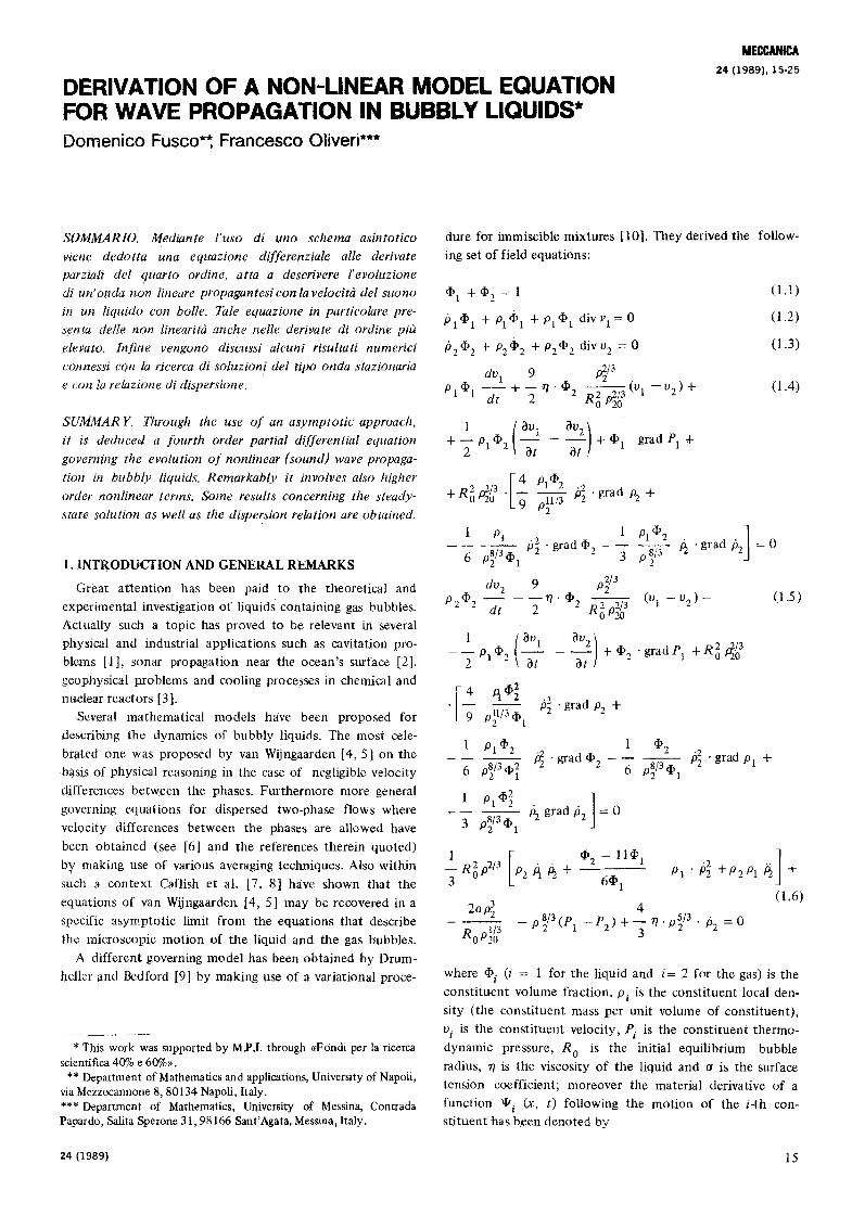
F i g u r e 1. S t e a d y w a v e p r o f i l e f o r R 0 = 0 . 4 n u n : / 3 = - 1 . 7 6 5 2 , 7 = - 2 . 8 5 2 4 , 6 = - 1 1 . 4 3 5 6 , # = - 0 . 1 2 2 3 , v = 0 . ~ 7 9 4 , 0 = - 0 . 1 6 4 8 .

wl

03-

-03'

sb

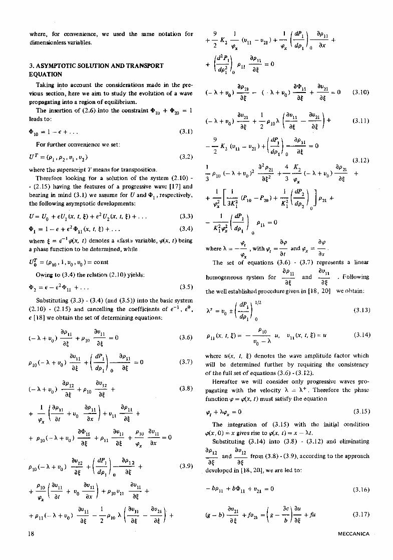
F i g u r e 2 . S t e a d y ~ c a v e p r o ~ e f o r R 0 = 0 . 6 r a m : / 3 = - 4 . 2 4 6 8 , 7 = ~ 5 ; 5 8 7 7 , fi = - 3 9 . 1 2 5 5 , # = - 2 9 4 2 6 , ~ = 0 . 2 8 4 5 , 0 = - 1 . 2 3 t 1.

20 MECCANICA

W

0.5-

~

Figu re 3. S t e a d y wave prof i le f o r R 0 = 0 .8 m m : / 9 = - - 7 . 5 8 8 6 , 7 = - - 3 . 3 5 3 ~ , 6 = - - 4 1 . 3 5 1 1 , / ~ = - - 7 . 1 7 6 9 , p = 0 . 1 7 9 3 , 0 ~= - - 2 2 , 1 6 1 .

W

0.5

-0.5-

sb C

F i g u r e 4 . S t e a d y wave prof i le f o r R 0 = 0 .9 r a m : / ~ - - - 9 . 6 0 9 7 , 3 ' = - 2 . 4 7 2 1 , 6 = - - 3 8 . 8 0 8 6 , ~t = - - 9 . 3 9 2 0 , ~ -~ 0 . 1 5 5 6 , 0 -- - - 2 - ~ 8 6 9 .

24 (1989) 21

W

0.5-

-0.5"

s'o C

F i g m e 5. S teady wave prof 'de for R 0 = 1 mm: /3 = - 11 .8669 , 7 = - 1 .8560, 5 = -- 3 6 0 , 5 3 6 , # = - 11 .7601 , ~, = 0 .1306 , 0 = -- 2 .9139 .

W

O.S ~

0

-0.5H

s'o

Figure 6 . S teady w a v e prof 'de fo r R o = 2 nun : ~ = - - 4 7 . 4 8 1 2 , 7 = - - 0 . 2 9 0 9 , 5 = - - 2 4 ~ 0 4 0 , # = - - 4 7 . 6 7 6 7 , v = 0 .6 8 8 6 , 0 = - - 5 .9052.

22 MECCANICA

w I

-0.5'

s'0

F i g u r e 7 . S t e a d y w a v e p r o f d e f o r R o = 3 m m : / ] = - - 1 0 6 . 8 3 3 , 7 = - - 0 . 1 1 8 7 , 6 = ~ 2 3 9 8 5 6 , / ~ = - - 1 0 7 . 2 8 6 , v = 0 . 0 4 5 7 , 0 = - - 8~8603 .

W

0.5"

-0.5"

F i g u r e 8 . S t e a d y w a v e p r o f i l e f o r R 0 = 4 m m : / ~ = , 1 8 9 . 9 2 6 , 7 = - - 0 , 0 7 6 2 , ~ = - - 2 6 . 3 5 8 2 , / ~ = - - 1 9 0 . 7 3 2 , ~ = 0 . 0 3 4 3 , 0 = - - 1 1 . 8 1 4 9 .

24 (1989) 23

F(k ) = -- 3 + (5 - la ~ + v3)k 2 + (O"l - ~5)k 4 > 0

(respectively: F( k ) < (0).

It is simple matter to see that we are led to linear sta-

bility when k 1 < k < k~ where k 1 a n d k 2 denote the (po-

sitive) roots of F(k).

It seems to us of a certain interest to point out the ranges

of the wavenumber k giving rise to F(k) < 0 in correspon-

dence to the values 3, % 5, ta, v, and 0 eonnected with the

model physical situation which has been assumed above

for investigating the behaviour of the steady-state solution

of (3:20). Therefore the values of k 1 and k 2 related to the

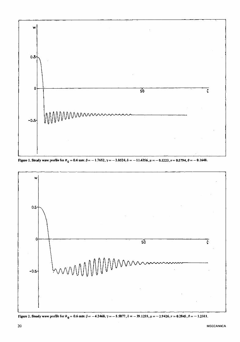
different choices of R 0 are listed below:

R 0 = 0.4 mm, k 1

R 0 = 0.6 mm, k 1

R 0 = 0.8 mm, k 1

R 0 = 0.9 mm, k 1

R 0 = 1 mm, k 1

R 0 =-2 mm, k 1

R 0 = 3 mm, k 1

R 0 = 4 ram, k 1

= 0.3877, k 2 = 1.2861

=0 .2768 , k 2 = 1.7537

= 0.3415, k 2 = 2.0905

= 0.3950, k 2 = 2.2252

= 0.4539, k z = 2.3489

= 1.1234, k 2 = 3.3157

= 1.7454, k 2 ~ 4.0381

= 2.2205, k 2 = 4.6181

5. CONCLUSIONS AND FINAL REMARKS

In this paper we considered the governing system of

equations derived by Drumheller and Bedford [9] for de-

scribing a gas-liquid mixture. Thus, within the theoretical

framework of the <<wave hierarchies>> studied by Whitham

[16] and Fusco [15], by means of a suitable asymptotic

approach we deduced a fourth order transport e~luation rul-

ing the propagation of nonlinear (sound) waves in bubbly

liquids.

In deriving this equation we took explicitly into account,

as the model proposed in [9] does, the diffusion effects

of the bubbles relative to the liquid as well as we assumed

that the gas volume fraction 42 , though small, was not

negligible. These leading assumptions gave rise to the higher

order nonlinear terms which make our model equation

different from other fourth order evolution equations derived

for gasqiquid mixtures (see for example [19]). In order to

investigate the travelling wave solutions to (3.20) we made

use of numerical integrations performed in connection

with a given model physical situation.

The results of the. calculations show that our equation

can admit either oscillatory or monotons' shock wave solu-

tions as the standard KdVB equation does. However, as

shown in figures 2 and 3, in the present case also wave

profiles exhibiting non-monotoniei ty of oscillation ampli-

tude seem to be possible.

To our own knowledge, unlike the wave behaviours com-

patible with the KdVB equation, the wave profiles of the

type shown in figures 2 and 3 have not been observed yet

in bubbly liquids. However, as pointed out in [23] there

are. some physical cases where a discrepancy between the

theoretical predictions based upon the KdVB equation

and experimental results occurs. Hence, apart from its

intrinsinc mathematical interest, the model equation (3.20),

despite of the complexity of the coefficients therein invol-

ved, should prove to be a suitable basis for experimental

studies which could verify or disprove the correctness of

the underlying postulates of the governing system proposed

in [9].

ACKNOWLEDGEMENT

The authors would like to thank the Referees for their

valuable criticism and suggestions to a previous draft of the

paper.

APPENDIX

The expressions of the constants b, c, d, e, f, g, m, n

and r which appear in the set of equations (3.16) - (3.19)

and in (3.21) are:

b = X - %

1 c = - - 010( - ~, + 00)2

3

4 d = - - - - ~ ' K 2 ( - X + t~ 0)

e - + o

9 - - K 2 1"= 2

1

g = 2 p1~

m = 2Pl 0

" = (o0_

6c 9c 2 b r = + - -

bm bern m

+ 2Ol0

Furthermore the coefficients a, ~, 7, 5, ~, v, 0 of the

transport equation (3.20) are given by:

n Ol =

rn

6c 9 c 2 b 2 9c2d 3 = - - + -

fro b2 frn fin beZm

dg 2 9c2d 9c 2 ",[= +

elm b 2 elm b f 2m

3cez b 2 d bdg 6cd + - - - - + + - -

b 2 frno efm elm elm

9c2g 2ez

b2 f2m fmo

6bc 6cg + - -

f2m f2m

+ -

2 4 M E C C A N I C A

b 3 b2g b 2 ez 9c 3 3cz

- f 2-----m + ~ + 3cfm-----~ + - - be2m b mo

bcg b 2 dg bdg 2 . 3cdg 2 6 - +

ef2m e2f2rn bef2rn

bg 3 beg 2 z b 2 egz + + ~ +

f 3 m f 3 m 3cf2mo

2eg2z bdgz dgz 3c 2 + - - + - - + ~ + ~

bfmo 3cfmo bfmu efm

9c2dg 3c2g 9c 3 9c 2 + - - + - -

b 2 e f2m befm

18c2g 362c

+ b--7 m +

eg2 z 3cez _ _ - - _{_

f 2 m o b f 2 m v

cz bz

bmu 3too

efm

2b2g 2

b2 efm f 3 m

3bcg 3cg 3 + - -

f 3 m

3cegz

3 ~ 2 m 0 "

b3g

f3 m +

2b 2 eg 2 z +

3 ~ 2 m u

3bcd 9c2d

~ 2 m b ~ 2 m

9c2g 2 - - + - - +

b2 f3m

3cg 3 bez

bf3m f 3 m f 2 m v

dz 3cdz - - + - - + fmo b2fmo

+

b2 f 2 m 0

3c2z

bernv

d ez

e �9 3co

c dz 1 7 = ~ - -

e 3co

z

0 -

3v

where we made the posit ions:

b3e o = +

+ 3el 2

2b 2 eg beg 2 be eg 2 2eg

3cf2 3cf2 + f2 bf2 f 2

bdg dg d b c + +

3cf by f 3 b

b 3 d 2b 2 dg bdg 2 3bcd 3cdg 2

z e f 2 + e f 2 e f 2 + e f 2 + be f 2

b2 c cg 2 bcg cg 2 3e 2 3c2g 3b2c _ - - + - - + _ _ + .... + + ~ _

e f e f e f e f e f bey f 3

3cg 3 9bcg 9cg z b 4 3b3 g

bf3 f 3 f 3 f3 f 3

3bZg z bg 3 _ ~ q L - -

f 3 f 3

bZd

3of

6cdg

ef 2

Received: September 3, 1987; in revised version: August 30, 1988.

R E F E R E N C E S

[ 1 ] PLESSET M.S., PRO~ERETH A., Bubble dynamics and cavitation, Ann. Rev. Fluid. Mech., 9, 1977, pp. 145-185.

[2] MEDWlN H., Acoustic fluctuations due to microbubbles in the near surface ocean. J. Acoust. Soc. Am.,56, 1974, pp. 1100- 1104.

[3] WALCHLI I{., WESf JAM., Heterogeneous water cooled reactors, in Reactor Handbook, vol. IV, Engineering, edited by S. McLain and J. H. Martens. Interscience, New York, 1964.

[4] van WIJNGAARDEN L., On the equations of motion for mixtures of liquid and gas bubbles. J. Fluid Mech., 33, 1968, pp. 465-474.

[5] van WIJNGAARDEN L., One-dimensional flow of liquids contain- ing small gas bubbles. Ann. Rev. Fluid Mech., 4, 1972, pp. 369-396.

[6] B/ESHEUVEL A., van WIJNGAARDEN L., Two-phase flow equa- tions for a dilute dispersion o f gas bubbles in liquid. J. Fluid Mech., 148, 1984, pp. 301-318.

[7] CAFLISH R.E., MIKSlS MJ., PAPANICOLAU G.C., TING L., Effective equations for wave propagation in bubbly liquids. J. Fluid Mech. 153, 1985, pp. 259-273.

[8] CAFLISH R.E., MIKSlS MJ., PAPANICOLAU G.C., TING L., Wave propagation in bubbly liquids at finite volume fraction. J. Fluid Mech., 160, 1985, pp. 1-14,

[9] DRUMHELLER D.S., BEDFORD A., A theory of bubbly liquids. J. Acoust. Soc. Am., 66, 1979, pp. 197-208.

[10] BEDFORD A., DRUMHELLER D.S., A variational theory of immiscible fluid mixture. Arch. Rat. Mech. Anal., 68, 1978, pp. 37-51.

[11] DRUMHELLER D.S., BEDFORD A., A thermomeehanical theory for reacting immiscible mixture. Arch. Rat. Mech. Anal. 73, 1980, pp. 257-284.

[12] DRUMHELLER D.S., BEDFORD A., A theory of liquids with

vapor bubbles. J. Acoust. Soc. Am., 67, 1980, pp. 186-200. [13] KUZNETSOV V.V., NAKORYAKOV V.E., POKUSAEV B.G.~

SHREIBER I.R., Liquid with gas bubbles as an example of a Korteweg~leVries-Burgers medium JETP Lett., 23, 1976, pp. 172-176.

[14] KUZNETSOV V.V., NAKORYAKOV V.E., POKUSAEV B.G., SHRE]BER I.R., Propagation of pert~zrbations in a gas-liquM mixture, J. Fluid Mech., 85, 1978, pp. 85-96.

[15] Fusco D., Some comments on wave motions described by non-homogeneous quasi-linear first order hyperbolic systems. Meccanica, 17, 1982, pp. 128-137.

[16] WH1THAM G.B., Linear and nonlinear waves. John Wiley and Sons, New York, 1974.

[17] GERMAIN P., Progressive waves. Jber DGLR, 1971. Koln, pp. I 1-39.

[18] BOILLAT G., Ondes asymptotiques non linEaires. Ann. Mat. Pura Appl., 61, 1976, pp. 31-44.

[19] NOORDZIJ L., van WIINGAARDEN L., Relaxation effects, caused by relative motion, on shock waves in gas-bubble/liquid mixtures. J. Fluid. Mech. 66, 1974, pp. 115-143.

[20] CHOQUET-BRUHAT Y., Ondes asymptotiques et approchEes pour des syst~mes d'equations aux derivdes partielles non lin& aires. J. Math. Pure appl., 48, 1969, pp. 117-158.

[21] KAWAHARA T., Formation of saturated solitons in a nonlinear dispersive system with instability and dissipation. Phys. Rev. Lett. 51, 1983, pp. 381-383.

[22] KIEFFER S.W., Sound speed in liquid-gas mixtures: waterair and water-steam. J. Geophys. Res., 82, 1977, pp. 2895-2904.

[23] DRUMHELLER D.$., KIPP M.E., BEDFORD A., Transient wave propagation in bubbly liquids. J. Fluid Mech., 119, 1982, pp. 347-365.

94 (1989) 25