Robust Arbitrage Conditions for Financial Markets

Derek Singh, Shuzhong Zhang

Department of Industrial and Systems Engineering, University of Minnesotasingh644@umn.edu, zhangs@umn.edu

Abstract

This paper investigates arbitrage properties of financial markets under distributional uncertainty using Wasser-stein distance as the ambiguity measure. The weak and strong forms of the classical arbitrage conditions are con-sidered. A relaxation is introduced for which we coin the term statistical arbitrage. The simpler dual formulationsof the robust arbitrage conditions are derived. A number of interesting questions arise in this context. One ques-tion is: can we compute a critical Wasserstein radius beyond which an arbitrage opportunity exists? What is theshape of the curve mapping the degree of ambiguity to statistical arbitrage levels? Other questions arise regardingthe structure of best (worst) case distributions and optimal portfolios. Towards answering these questions, sometheory is developed and computational experiments are conducted for specific problem instances. Finally someopen questions and suggestions for future research are discussed.

Keywords— arbitrage, statistical arbitrage, Farkas lemma, robust optimization, Wasserstein distance, Lagrangian duality

1 Introduction and Overview

1.1 The Characterization of Arbitrage in Financial MarketsFinancial arbitrage with respect to securities pricing is a fundamental concept regarding the behavior of financial markets

developed by Ross in the 1970s. A couple of his seminal papers include Return, Risk, and Arbitrage (Ross et al., 1973) andThe Arbitrage Theory of Capital Asset Pricing (Ross, 1976). In the author’s own words the arbitrage model or arbitrage pricingtheory (APT) was developed as an alternate approach to the (mean variance) Capital Asset Pricing Model (CAPM) (Sharpe,1964) which was itself an extension of the foundational work on Modern Portfolio Theory by Harry Markowitz (Markowitz,1952). Ross argued that APT imposed less restrictions on the capital markets as did CAPM such as its requirement that themarket be in equilibrium and its consideration of (only) a single market risk factor as measured by variance of asset returns.Recall that CAPM uses the security market line to relate the expected return on an asset to its beta or sensitivity to systematic(market) risk. APT, on the other hand, is a multi-factor cross sectional model that explains the expected return on an asset inlinear terms of betas to multiple market risk factors that capture systematic risk (Ross et al., 1973), (Ross, 1976).

The motivating idea behind APT is the no-arbitrage principle as characterized by the no-arbitrage conditions. This principleasserts that in a securities market it should not be possible to construct a zero cost portfolio that guarantees per scenario eithera riskless profit or no chance of losses, across all possible market scenarios. If this were the case, one would be able to makemoney from nothing, so to speak. Ross formulates the no-arbitrage conditions and via duality theory of linear programmingshows the equivalent existence of a state price vector to recover market prices (Ross et al., 1973). Existing results in theliterature (Delbaen and Schachermayer, 2006) have shown the equivalence between the single period and multi period no-arbitrage properties (on a finite probability space). To simplify the analysis, we focus on the discrete single period setting.

As a further refinement, the notions of weak and strong arbitrage were developed. A portfolio w∈Rn of n market securitiesis designated a weak arbitrage opportunity if w ·S0 ≤ 0 but Pr(w ·S1 ≥ 0) = 1 and Pr(w ·S1 > 0)> 0 for initial asset price vectorS0 and time 1 asset price vector S1. Similarly, a portfolio w ∈ Rn is designated a strong arbitrage opportunity if w ·S0 < 0 butPr(w ·S1 ≥ 0) = 1. In a discrete setting with s market states, given security price vector p ∈ Rn and payoff matrix X ∈ Rn×s, aweak arbitrage opportunity is a portfolio w ∈Rn that satistifes X>w 0 and p>w≤ 0. Similarly, a strong arbitrage opportunityis a portfolio w ∈ Rn that satistifes X>w ≥ 0 and p>w < 0. Note there are cases of weak arbitrage portfolios which are notstrong arbitrage portfolios (cf. e.g. LeRoy and Werner, 2014).

In a discrete setting, the well known Farkas Lemma can be used to characterize the property of (weak) strong arbitrage.The Farkas Lemma characterization says that security price vectors p exclude (weak) strong arbitrage iff given payoff matrixX (across all market scenarios) there exists a (strictly) positive solution q to p = Xq. The normalized state price vectorsq∗s = qs/∑s qs become the set of discrete risk neutral probabilities that defines the measure Q (cf. e.g. LeRoy and Werner, 2014).

1

arX

iv:2

004.

0943

2v1

[q-

fin.

PM]

20

Apr

202

0

The fundamental theorem of asset pricing (also: of arbitrage, of finance) equates the non-existence of arbitrage opportunities ina financial market to the existence of a risk neutral (or martingale) probability measure Q which can be used to compute the fairmarket value of all assets. A financial market is said to be complete if such a measure Q is unique (cf. e.g. Follmer and Schied,2011). The unique measure Q is frequently used in mathematical finance and the pricing of derivative securities in particular,in both discrete time (Shreve, 2005) and continuous time settings (Shreve, 2004).

In the context of distributional uncertainty, a natural question arises as to how to characterize the notion of arbitrage. Onewould presumably seek a balance of generality and practicality in developing a framework to study the arbitrage properties.Some structure is needed to develop intuition and understanding. On the other hand, too much structure could be restrictiveand limit useful degrees of freedom. The approach taken in this line of research is to start from the fundamental (weak andstrong) no-arbitrage conditions and investigate how the market model transitions from one of no-arbitrage to arbitrage or viceversa. Distributional uncertainty is characterized via the Wasserstein metric for a couple reasons. The Wasserstein metricis a (reasonably) well understood metric and a natural, intuitive way to compare two probability distributions using ideas oftransport cost. It is also a flexible approach that encompasses parametric and non-parametric distributions of either discreteor continuous form. Furthermore, recent duality results and structural results on the worst case distributions could help usto understand and/or quantify the market model transitions as well as measure (in a relative sense) the degree of arbitrage orno-arbitrage inherent to a given market model.

Logical reasoning dictates that it should be possible to distort a no-arbitrage measure into an arbitrage admissible measure.For a simple discrete example, consider a one-period binomial tree of stock prices where 0 < Sd < 1+ r < Su, pu + pd = 1,pu > 0 =⇒ pd > 0 are the conditions that characterize an arbitrage-free market (Shreve, 2005). If we now distort the aboveQ measure into a P measure such that pd = 0, it is clear to see that a zero cost portfolio that is long the stock and short ariskless bond will make profit with probability 1. So then, how “far” is this distorted measure P from the original no-arbitragemeasure Q? Can we safeguard ourselves within a ball of (only) arbitrage-free probability measures Q′ of distance at most δ

from the reference measure Q? What is the structure of the worst case distributions and optimal portfolios within this ball? Isthere a critical radius δ ∗ for this ball of arbitrage-free measures beyond which an arbitrage admissible measure is sure to exist?Alternatively, suppose the reference measure Q admitted arbitrage. What is the nearest arbitrage-free measure to this measure?Is that minimal distance, call it δ ∗g , computable? These questions are the motivation for the line of research conducted in thispaper. As mentioned above, this research uses the Wasserstein distance metric (cf. e.g. Villani, 2008). To the best of ourknowledge, this paper is the first to investigate these notions under the Wasserstein metric and develop a mixture of theoreticaland computational answers to these questions.

The contributions of this paper are as follows. Primal problem formulations for the classical and statistical arbitrage con-ditions (under distributional uncertainty using Wasserstein ambiguity) are developed. Using recent duality results (Gao andKleywegt, 2016), (Blanchet and Murthy, 2019), simpler dual formulations that only involve the reference arbitrage-free proba-bility measure are constructed and solved. The max-min and max-max dual problems are formulated as nonlinear programmingproblems (NLPs). The structure of the best (worst) case distributions is analyzed. A formal proof for the NP hardness of thedual no-arbitrage problem is also given. Using this theoretical machinery, the critical radii δ ∗, the best (worst) case distribu-tions, and/or optimal portfolios are computed for a few specific problem instances involving real world financial market data.The complementary problem to compute the minimal distance δ ∗g to an arbitrage-free measure for a reference measure thatadmits arbitrage is formulated and solved. We make use of the fundamental theorem of asset pricing to do this (cf. e.g. LeRoyand Werner, 2014; Follmer and Schied, 2011).

An outline of this paper is as follows. Section 1 gives an overview of the financial concepts of arbitrage and statistical arbi-trage as well as a literature review. Section 2 develops the main theoretical results to characterize arbitrage under distributionaluncertainty using Wasserstein distance. Section 3 extends this machinery to cover the notion of statistical arbitrage. Section4 presents applications of the theory developed in Sections 2 and 3. Section 5 gives formal proofs for the NP hardness of theno-arbitrage problem. Section 6 is a computational study of the arbitrage properties for a few specific problem instances andcomputes numerical solutions. Section 7 discusses conclusions and suggestions for further research.

1.2 The Characterization of Statistical Arbitrage in Financial MarketsStatistical arbitrage denotes a class of data driven quantitative trading and algorithmic investment strategies, for a set of

securities, to exploit deviations in relative market prices from their “true” distributions. Classical notions of statistical arbitrageopportunites involve estimation and use of statistical time series models (such as cointegration or kalman filter) to describestructural properties of asset prices such as mean reversion, volatility, etc. and help identify temporal deviations in marketprices that present trading and/or investment opportunites before the market “reverts” to its equilibrium behavior (Focardi et al.,2016). One particular sub-class of such strategies that is prevalent in both the literature and industry practice is known as pairstrading. The canonical example here is the coke vs. pepsi trade where one identifies a price dislocation and then simultaneouslyshorts the over-priced asset and buys the under-priced asset and waits for the relative prices to restore to equilibrium, and closesout the position, thus realizing a profit for the arbitrageur (Krauss, 2017).

2

Practitioners, such as investment banks and hedge funds, employ a wide array of professionals to work in multiple aspectsof this: such as trading systems design and technology support, data collection, model development, trade execution, riskmanagement, reporting, business development, and so on. The actual practice of statistical arbitrage typically involves amixture of art and science. The science component is reflected through the estimation and use of statistical time series modelsand incorporation of emerging trends in the academic literature and technology (for the practical aspects of trade execution andrisk management). The art component is reflected through incorporation of investment professionals knowledge, experience,and beliefs about financial markets’ current state and future outlook (Lazzarino et al., 2018).

Classical notions of statistical arbitrage “already” have an intrinsic notion of variability, hence their name. The motivationfor the line of research in this paper is to extend this notion to incorporate distributional uncertainty within the framework ofWasserstein distance and the corresponding duality results. In this sense, the objectives are analagous, with the topic of focusshifted from classical arbitrage to statistical arbitrage. The first steps are to define notions of statistical arbitrage and robuststatistical arbitrage and characterize their meaning. A survey of the literature reveals that no universal definition of statisticalarbitrage currently exists (Lazzarino et al., 2018). With that in hand, next steps are to quantify the best case (αbc) and worstcase (αwc) levels of statistical arbitrage as a function of the degree of distributional uncertainty, as represented by the radiusδ of the Wasserstein ball. A related, complementary, problem is how to find the nearest probability measure (to the original,reference measure) that guards against statistical arbitrage of level α close to 1.

1.3 Literature ReviewIn conducting the literature review for this research, not many references were found that have investigated the topic of

arbitrage under distributional uncertainty. From Section 1.1 above, one can see that considerable research has been done inacademic circles regarding the classical notions of arbitrage in financial markets. Indeed, several academic papers and financialtextbooks have been written that cover these topics from their origin in the 1970s until today. It was surprising to us, at least,to find only a few papers that address and/or extend the classical notions of arbitrage under the presence of some form ofdistributional uncertainty. This subsection gives an overview of what we found in the academic literature.

An earlier paper by Jeyakumar and Li (2011) took a Farkas Lemma approach to describe linear systems subject to datauncertainty in the form of bounded uncertainty sets. The authors develop a notion of a robust Farkas Lemma in terms of theclosure of a convex cone they call the robust characteristic cone. As an application of the lemma, they characterize robustsolutions of conic linear programs with data contained in closed convex uncertainty sets. Recently Dinh et al. (2017) appliedthe robust Farkas Lemma approach to characterize weakly minimal elements of multi-objective optimization problems withuncertain constraints. Note that weakly minimal elements correspond to the notion of optimal solution in the scalar (singletonvector) case. The authors remark that their results are consistent with existing literature in the scalar case.

One seminal paper of note by Ostrovskii used the total variation (TV) metric to characterize a radius δTV such that allprobability measures Q′ within this distance from a weak arbitrage-free reference measure Q are also weak arbitrage-free.The author remarks that δTV can be interpreted as the minimal probability of success that a zero cost initial portfolio w ∈ Rn

achieves positive value w · S1 at time 1. The additional constraint on the selected portfolio w is that it must have a strictlypositive probability of profit under the reference measure P. This allows δTV > 0 to hold. This lemma is proven using toolsfrom probability theory and real analysis. The main result relating δTV to the minimal probability of success is established viaproof by contradiction (Ostrovski, 2013). The bound appears to be tight although this result is not proven in the paper.

The author remarks that the probability measures Q and Q′ could have different support and/or generate different probabilityspaces. Furthermore, Ostrovski describes the no-arbitrage conditions and computes the critical radius δTV for a one-periodbinomial and trinomial tree respectively. The conditions for the one-period binomial tree are given in Section 1.1 above. Thecorresponding radius δTV is min(pu, pd). For the one-period trinomial tree, different configurations are possible. Let qd ,qm,qudenote the one-period transition probabilities to the down, middle, and up nodes respectively. For the case Sd < Sm < 1+r < Suthe trinomial tree would allow arbitrage iff qd = qm = 0 or qu = 0. In the first case, the TV distance between the binomial andtrinomial trees would be max(1− pu, pd) = max(pd , pd) = pd . In the second case it would be max(pu,qm, |pd − qd |) ≥ pu.Thus the trinomial model would be arbitrage-free if the TV distance to the binomial model were less than min(pu, pd). Theother cases Sd < Sm = 1+ r < Su and Sd < 1+ r < Sm < Su can be handled similarly (Ostrovski, 2013). While these results aretractable it was not clear (to us) how to apply these results to develop a dual formulation to study the market model transitionsfrom no-arbitrage to arbitrage or vice versa. Furthermore, total variation distance has been described as a strong notion ofdistance in the academic literature. Given our motivation to avoid (strong) restrictions in our characterization of robust no-arbitrage markets, it would seem that a different notion of distance between probability measures might be more appropriate.

A recent paper by Bartl et al. (2017) explicitly incorporates a no-arbitrage constraint directly into the worst case Europeancall option pricing problem under Wasserstein ambiguity. We consider this problem from a different perspective in this paper,namely we restrict the Wasserstein ball of probability measures to implicitly consider only those measures which are arbitrage-free without the need to enforce an explicit constraint. In Section 2, the theoretical machinery to compute a critical radius δ ∗w(s)is developed to pursue this approach. Simpler worst case option pricing formulas (that omit the explicit no-arbitrage constraint)

3

are derived as well.Finally, another recent paper by the same author (Bartl et al., 2019) investigates the robust exponential utility maximization

problem in a discrete time setting. The worst case expected utility is maximized under a family of probabilistic models ofendowment that satisfy no-arbitrage conditions by assumption. The authors show that an optimal trading strategy exists andthey provide a dual representation for the primal optimization problem. Furthermore, the optimal value is shown to converge tothe robust superhedging price as the risk aversion parameter increases.

1.4 Arbitrage FrameworkThis section lays out the foundations for our framework to investigate the arbitrage properties under distributional uncer-

tainty. Recall the approach taken here is to start from the classical no-arbitrage conditions and introduce a notion of distribu-tional uncertainty via the Wasserstein distance metric. As such, we include definitions for these terms as well as commentaryon some important results:

(i) definitions for no-arbitrage and statistical arbitrage conditions;

(ii) Lagrangian duality to formulate the dual problem for robust arbitrage in financial markets;

(iii) existence and structure of worst case distributions;

(iv) computation of Wasserstein distance between distributions.

1.4.1 Weak and Strong No-Arbitrage (NA) Conditions

The set of admissible portfolio weights for the weak no-arbitrage conditions is

Γw(S0) := w ∈ Rn : w ·S0 = 0; w 6= 0. (WW)

The set of admissible portfolio weights for the strong no-arbitrage conditions is

Γs(S0) := w ∈ Rn : w ·S0 < 0. (SW)

The no-arbitrage condition to be evaluated under probability measure Q in both cases is Pr(w · S1 ≥ 0) = EQ[1w·S1≥0 ] < 1.Note that portfolio weight vectors w satisfy the positive homogeneity property (of degree zero) since Pr(w ·S1≥ 0) = Pr(w ·S1≥0) for w = cw and c > 0. It is the proportions of the holdings in the assets that distinguish w vectors, not their absolute sizes.Weak arbitrage requires two conditions to hold: Pr(w · S1 ≥ 0) = 1 and Pr(w · S1 > 0) > 0. The second condition is noteasily incorporated into the duality framework of this paper and hence it is omitted. Consequently the critical radius δ ∗w that isdeveloped in Section 2 may not be tight. Strong arbitrage requires just one condition hence the bound δ ∗s will be tight.

For a given measure Q, no weak arbitrage means that supw∈ΓwEQ[1w·S1≥0 ] < 1. Similarly, for a given measure Q, no

strong arbitrage means that supw∈ΓsEQ[1w·S1≥0 ]< 1. The empirical measure, QN , is defined as QN(dz) = 1

N ∑Ni=11s(1,i)(dz).

To simplify the notation, the leading subscript on s(1,i) is suppressed and going forward we refer to the realization of time 1asset price vector s(1,i) as just si. In the context of this work, the uncertainty set for probability measures is Uδ (QN) = Q :Dc(Q,QN) ≤ δ where Dc is the optimal transport cost or Wasserstein discrepancy for cost function c (Blanchet et al., 2018).The definition for Dc is

Dc(Q,Q′) = infEπ [c(X ,Y )] : π ∈ P(Rn×Rn),πX = Q,πY = Q′where P denotes the space of Borel probability measures and πX and πY denote the distributions of X and Y . Here X denotesasset prices SX ∈Rn and Y denotes asset prices SY ∈Rn respectively. This work uses the cost function c where c(u,v)= ‖u−v‖2.

1.4.2 Note on Equivalence of Single and Multi Period NA

For clarity we cite the following result from the literature (Delbaen and Schachermayer, 2006). Let S = (St)Tt=0 be a discrete

price process (with unit increments and T ∈ N) on a finite probability space (Ω,F ,P). Then the following are equivalent:

(i) S satisfies the no-arbitrage property;

(ii) For each 0 ≤ t < T , we have that the one-period market (St ,St+1) with respect to the filtration (Ft ,Ft+1) satisfies theno-arbitrage property.

Further detail on the equivalence of single and multi period no-arbitrage can be found in e.g. LeRoy and Werner (2014).As our focus in this paper is on the discrete single period setting, the above relationship suffices. One direction for furtherresearch would be to consider the robust no-arbitrage properties in a multi period continuous time setting for a suitable class ofadmissible trading strategies. A more general version of the fundamental theorem of asset pricing applies there. See Delbaenand Schachermayer (2006) for additional detail on this topic.

4

1.4.3 Weak and Strong Statistical Arbitrage (SA) Conditions

To characterize the situation where a profitable trading opportunity is highly likely yet not necessarily certain, we introducea notion of statistical arbitrage. Recall that no universal definition of statistical arbitrage currently exists (Lazzarino et al.,2018). Towards that end, we propose using a relaxation of the classical arbitrage conditions to define a notion of statisticalarbitrage. In particular, let us write the best case (bc) statistical arbitrage (of level αbc ∈ (0,1)) condition under probabilitymeasure Q as Pr(w · S1 ≥ 0) = EQ[1w·S1≥0 ] ≤ αbc. The set of admissible portfolio weights for the weak (strong) conditionis w ∈ Γw(s) as before (see Section 1.4.1). Intuitively, the best case statistical arbitrage condition says that it should not bepossible to construct a zero (or negative) cost portfolio that returns either a profit or no chance of losses with probability αbc

close to 1. In the limit αbc→ 1 one recovers the classical arbitrage condition. Similarly, the worst case (wc) condition (of levelαwc ∈ (0,1)) is Pr(w ·S1 ≥ 0) = EQ[1w·S1≥0 ]≥ αwc. Probability αwc close to 0 describes a no-win situation.

1.4.4 Restatement of Lagrangian Duality Result

In Section 2 we formulate the primal stochastic optimization problem for distributionally robust arbitrage-free markets. Asin our earlier work (Singh and Zhang, 2019) a key step in the approach is to use recent Lagrangian duality results to formulatethe equivalent dual problem. The dual problem is much more tractable than the primal problem since it only involves thereference probability measure as opposed to a Wasserstein ball of probability measures (of some finite radius). This allowsus to solve a maximin optimization problem under the original empirical measure defined by the selected data set. A briefrestatement of this duality result follows next.

For real valued upper semicontinuous objective function f ∈ L1 and non-negative lower semicontinuous cost function csuch that (u,v) : c(u,v)< ∞ is Borel measurable and non-empty, it holds that (Blanchet et al., 2016)

supQ∈Uδ (QN)

EQ[ f (X)] = infλ≥0

[λδ +1N

n

∑i=1

Ψλ (xi)]

whereΨλ (xi) := sup

u∈dom( f )[ f (u)−λc(u,xi)].

The primal problem (LHS above) is concerned with the worst case expected loss for some objective function f with respect to aWasserstein ball of probability measures of finite radius δ . The Wasserstein ball is used to reflect some (real world) uncertaintyabout the true underlying distribution for random variable (or vector) X . Note that the primal problem is an infinite dimensionalstochastic optimization problem and thus difficult to solve directly. The simplicity and tractability of the dual problem (RHSabove) make it quite attractive as an analytical and/or computational tool in our toolkit.

Further details, including proofs and concrete examples, can be found in the papers by Blanchet and Murthy (2019), Gaoand Kleywegt (2016), and Esfahani and Kuhn (2018). These authors independently derived these results around the sametime although Blanchet and Murthy (2019) did so in a more general setting. The duality result has been applied by the aboveauthors and others in several papers on topics in data driven distributionally robust stochastic optimization such as robustmachine learning, portfolio selection, and risk management. For these types of robust optimization problems, the incorporationof distributional uncertainty can be viewed as adding a penalty term (similar to penalized regression) to the optimal solution(Blanchet et al., 2018). This gives us a nice intuitive way to think about the cost of robustness.

1.4.5 Characterization of Worst Case Distributions

Simply put, the set of worst case (wc) distributions (when non-empty) can be defined as WC( f ,δ ) := Q∗ : EQ∗ [ f (X)] =supQ∈Uδ (QN)

EQ[ f (X)]. Another recent set of results from the literature describes the existence and structure of the worstcase distribution(s) when they exist (Blanchet and Murthy, 2019), (Gao and Kleywegt, 2016), (Esfahani and Kuhn, 2018). Theboundedness conditions for existence are tied to the growth rate κ := limsup

d(X ,X0)→∞

f (X)− f (X0)d(X ,X0)

for fixed X0 and the value of the dual

minimizer λ ∗. For empirical reference distributions, supported on N points, such that WC( f ,δ ) is non-empty, there exists aworst case distribution that is another empirical distribution supported on at most N+1 points. This worst case distribution canbe constructed via a greedy approach. For up to N points, they can be identified as solving x∗i ∈ argminx∈dom( f )[λ

∗c(x,xi)−f (x)]. At most one point has its probability mass split into two pieces (according to budget constraint δ ) that solve x∗i0 ,x

∗∗i0 ∈

argminx∈dom( f )[λ∗c(x,xi0)− f (x)]. Details can be found in Gao and Kleywegt (2016). For our problem setting, the growth

rate conditions are satisfied and hence we proceed to formulate and then apply a greedy algorithm (see Section 2.2) to computethe worst case distribution for a concrete example in Section 5. A similar example from the literature, which uses a greedyalgorithm to compute the minimal (worst case) membership to a given set C, is covered in (Gao and Kleywegt, 2016). Note thatother worst case distributions can be constructed with different support sets and/or probability mass functions (PMFs). It can

5

be insightful to examine how the reference distribution can be perturbed for a given objective f as δ varies. See Section 2.2 forspecific commentary on the structure and construction of the worst case distribution(s) for the robust NA problem.

1.4.6 On Computing Wasserstein Distance

This section introduces some standard and recent results on computing Wasserstein distance between distributions. Therecent results are focused on discrete distributions since our problems of interest are data driven. The standard results (below) aretaken from the online document by Wasserman (2017). Wasserstein distance has simple expressions for univariate distributions.The Wasserstein distance of order p is defined over the set of joint distributions P with marginals Q and Q′ as

Wp(Q,Q′) =(

infπ∈P(X ,Y )

∫‖x− y‖p dπ(x,y)

)1/p

.

Note that in this work we consider Wasserstein distance of order p = 1. When d = 1 there is the formula

Wp(Q,Q′) =(∫ 1

0|F−1(z)−G−1(z)|p dz

)1/p

.

For empirical distributions with N points, there is the formula using order statistics on (X ,Y )

Wp(Q,Q′) =

(N

∑i=1‖X(i)−Y(i)‖p

)1/p

.

Additional closed forms are known for: (i) normal distributions, (ii) mappings that relate Wasserstein distance to multiresolutionL1 distance. See Wasserman (2017) for details. This concludes the brief survey of standard (closed form) results.

For discrete distributions, at least a couple of methods have been recently developed to compute approximate and/or (inthe limit) exact Wasserstein distance. The commentary on these methods is taken from Xie et al. (2018). For distributions withfinite support, and cost matrix C, one can compute W (Q,Q′) := minπ〈C,π〉 with probability simplex constraints using linearprogramming (LP) methods of O(N3) complexity. An entropy regularized version of this, using regularizer h(π) :=∑πi, j logπi, jgives rise to the Sinkhorn distance

Wε(Q,Q′) := minπ〈C,π〉+ εh(π)

which can be solved using iterative Bregman projections via the Sinkhorn algorithm. However, the authors comment thatcertain problems (such as generative model learning and barycenter computation) experience performance degradation for amoderately sized ε but opting for a small size can be computationally expensive. To address these shortcomings, they developtheir own approach called inexact proximal point method for optimal transport (IPOT). The proximal point iteration takes theform

π(t+1) = argmin

π

〈C,π〉+β(t)Dh(π,π

(t))

where β denotes a parameter of the method and Dh denotes the Bregman divergence based on the entropy function. Substitutionfor Bregman divergence gives the form

π(t+1) = argmin

π

〈C−β(t) logπ

(t),π〉+β(t)h(π).

It turns out that this iteration can also be solved via the Sinkhorn algorithm. However the authors propose an inexact methodthat improves efficiency while maintaining convergence. See Xie et al. (2018) for details.

2 Theory: Robust Arbitrage Conditions for Financial MarketsThis section develops the theory for robust arbitrage in financial markets. In Section 2.1, the primal problem is formulated

using classical notions of arbitrage as discussed in Section 1.4.1. The dual problem is formulated using the Lagrangian dualityresult from Section 1.4.4. Note that the dual problem is a maximin stochastic optimization problem. The inner optimizationproblem (evaluating Ψλ ,w) can be solved analytically using the Projection Theorem (Calafiore and El Ghaoui, 2014). Themiddle optimization problem (evaluating the dual objective function over infλ≥0) can be solved via execution of a simple linearsearch algorithm over a finite set of points. The outer optimization problem (evaluating over supw∈Γw(s)

) can be formulated asan NLP. Finally, the middle and outer problems can be solved jointly via a maximin NLP approach.

Section 2.2 gives details on the worst case distributions and Sections 2.3 and 2.4 show how to incorporate portfolio restric-tions (such as short sales) in a straightforward manner. Section 2.5 introduces the complementary problem of how to find thenearest arbitrage-free measure to the arbitrage admissible reference measure. This machinery gives us a practical approach toexplore applications of our framework for robust arbitrage.

6

2.1 Robust Weak and Strong No-Arbitrage (NA) ConditionsThe robust weak no-arbitrage conditions can be expressed as

supw∈Γw

supQ∈Uδ (QN)

EQ[1w·S1≥0 ]< 1 (WP)

where Γw is defined in WW. Note the indicator function 1w·S1≥0 on closed set w ·S1 ≥ 0 is upper semicontinuous hence wecan apply the duality theorem (see Section 1.4.4) to obtain the dual formulation

supw∈Γw

infλ≥0

[λδ +1N

N

∑i=1

Ψλ ,w(si) ]< 1 (WD)

where Ψλ ,w is defined, in terms of cost function c, as Ψλ ,w = sups∈Rn [1w·s≥0−λc(s,si) ]. Similarly, for the robust strongno-arbitrage conditions

supw∈Γs

supQ∈Uδ (QN)

EQ[1w·S1≥0 ]< 1 (SP)

where Γs is defined in SW, the dual formulation is

supw∈Γs

infλ≥0

[λδ +1N

N

∑i=1

Ψλ ,w(si) ]< 1. (SD)

2.1.1 Inner Optimization Problem

The objective here is to evaluate Ψλ ,w in closed form. There are two cases to consider.

Case 1.1w·si≥0 = 1 =⇒ Ψλ ,w(si) = 1−λ ·0 = 1 which is optimal.

Case 2.1w·si≥0 = 0 =⇒ Ψλ ,w(si) = [1−λc(s∗i ,si)]

+ where s∗i = argmin‖s− si‖2 is optimal.

By the Projection Theorem (Calafiore and El Ghaoui, 2014), ‖s∗i − si‖2 =|w>si|‖w‖2

=⇒ Ψλ ,w(si) = [1−λci]+ for

ci =|w>si|‖w‖2

∈ Rn+.

Proposition 1.1N

N

∑i=1

Ψλ ,w(si) = K0(w)+K1(λ ,w)

where K0(w) = 1N ∑

Ni=11w·si≥0 and K1(λ ,w) = 1

N ∑Ni=11w·si<0[1−λci]

+ for ci =|w>si|‖w‖2

∈ Rn+.

Proof. This follows by a straightforward application of the two cases above.

2.1.2 Middle Optimization Problem

Remark 1. In this subsubsection, the dependency of λ ∗ on (w,δ ) is suppressed to ease the notation.

Now the objective is to evaluate infλ≥0 H(λ ) := [λδ +K0(w)+K1(λ ,w) ]. Since H(λ ) is a convex function of λ , the firstorder optimality condition suffices to determine λ ∗ = argminλ≥0 H(λ ). Note that H(λ ) may have kinks so we look for λ ∗ suchthat 0 ∈ ∂H(λ ∗). Following the approach in our earlier work (Singh and Zhang, 2019), we arrive at the following result.

Proposition 2. Let λ ∗ = supλ≥0λ : δ − 1N [∑i∈J+1 (λ )1w·si<0ci]≤ 0= infλ≥0λ : δ − 1

N [∑i∈J1(λ )1w·si<0ci]≥ 0,where

J+1 (λ ) = i ∈ 1, . . . ,N : 1−ciλ > 0, J1(λ ) = i ∈ 1, . . . ,N : 1−ciλ ≥ 0. In the degenerate case, where supλ≥0 is takenover an empty set, select λ ∗ = 0 =⇒ H(λ ∗) = 0.

Proof sketch. This result follows from writing down the first order conditions for left and right derivatives for convex objectivefunction H(λ ). For each additional index i ∈ J+1 (J1) such that at least one indicator function is true, we pick up an additional citerm in the left (right) derivative. Search on λ (from the left or the right) until we find λ ∗ such that 0 ∈ ∂H(λ ∗).

7

Proof. The first order optimality condition says

δ − 1N ∑

i∈J+1 (λ )

1w·si<0ci ≤ 0≤ δ − 1N ∑

i∈J1(λ )

1w·si<0ci.

Note the LHS is an increasing function in λ . Hence one can write

λ∗ = sup

λ≥0λ : δ − 1

N ∑i∈J+1 (λ )

1w·si<0ci ≤ 0.

Similarly the RHS is also an increasing function in λ . Equivalently, one can write

λ∗ = inf

λ≥0λ : δ − 1

N ∑i∈J1(λ )

1w·si<0ci ≥ 0.

Proposition 3. Equivalently, λ ∗ can be computed via a linear seach over 1ci as in Algorithm 1 (listed below).

Proof. The break points for J1(J+1 ) are ci : i ∈ 1, . . . ,N. Observe that the only possible candidates for λ ∗, as given inProposition 2.2, are 1

ci: i ∈ 1, . . . ,N or 0. One can sort and relabel the ci to be in increasing order. Note that (1− c jλ ) >

0 =⇒ (1− ciλ ) > 0 ∀ ci ≤ c j. Thus m ∈ J1(J+1 ) =⇒ 1, . . . ,m ∈ J1(J+1 ). Search backwards to find the smallest indexk∗ ∈ 1, . . . ,N such that ∑

k∗i=11w·si<0ci ≥ Nδ . If no such index k∗ is found, return λ ∗ = 0 else return λ ∗ = 1

ck∗.

Algorithm 1: Linear Search over 1ci to compute λ ∗

Input: 1ci, w , si , N , δ

Output: λ ∗ = supλ≥0λ : δ − 1N [∑i∈J+1 (λ )1w·si<0ci]≤ 0= infλ≥0λ : δ − 1

N [∑i∈J1(λ )1w·si<0ci]≥ 01 Set Q∗ = QN2 Sort ci Increasing3 Compute Vk where Vk := ∑

ki=11w·si<0ci

4 k = N5 if Vk < Nδ then6 return λ ∗ := 0

7 else8 while k ≥ 1 and Vk ≥ Nδ do9 k = k−1

10 k∗ = k+111 return λ ∗ := 1

ck∗

2.1.3 Outer Optimization Problem

The weak no-arbitrage conditions can now be expressed as

vw(δ ) := supw∈Γw

λ ∗(w,δ )δ +K0(w)+K1(λ∗(w,δ ),w)< 1. (WD2)

Similarly, for the strong no-arbitrage conditions

vs(δ ) := supw∈Γs

λ ∗(w,δ )δ +K0(w)+K1(λ∗(w,δ ),w)< 1. (SD2)

The authors are not aware of any such pairing of mixed integer nonlinear program (MINLP) formulation and solver thatcan return the (global) optimal values vw(s)(δ ) for arbitrary problem instances. Our attempts at such an MINLP formu-lation to be solved using Neos / Baron MINLP solvers (Tawarmalani and Sahinidis, 2005) and/or Neos / Knitro solvers(Byrd et al., 2006) were successful on small but not large problem instances. Difficulties were encountered in finding fea-sible solutions and/or returning optimal solutions. Given the findings above, our original solution strategy was revised tofocus on solving an equivalent NLP maximin problem formulation to local optimality using the Matlab fminimax solver andthe identity maxx mink Fk(x) = −minx maxk(−Fk(x)). The equivalent formulation is constructed from the observation thatλ ∗ ∈ 1

ck: k ∈ 1, . . . ,N∪λ0 := 0. Developing a global solution strategy would be an interesting area for further research.

8

Theorem 1. vw(δ ) is approximated by the (global) solution to nonlinear program (NLP) N WNA (listed below).

The constraints on variables below, with index i, apply for i ∈ 1, . . . ,N, although this is suppressed. Also recall that weightvectors w satisfy homogeneity, hence the use of “big M” to express w ∈ Γw(s) is appropriate.

>

w∈Rn maximize<

b minλk : k∈0,1,...,N

Fk(w) := λkδ +1N

[ N

∑i=1

1w·si≥0+N

∑i=1

z+i 1w·si<0

]vw(δ ) =

subject to ci =|w>si|‖w‖2

,

λk =1ck∀k ∈ 1, . . . ,N,

λ0 = 0,|wi| ≤M,

w ·S0 = 0,n

∑j=1|w j| ≥ ε,

zi = [1−λkci]

(1)

Proof. The NLP formulation follows from equation WD2 and the fact that λ ∗ ∈ 1ck

: k ∈ 1, . . . ,N∪λ0 := 0.

Corollary 1. vs(δ ) is approximated by the solution to NLP N SNA (described next). N SNA is very similar to N WNA. Onejust needs to omit the ∑

nj=1 |w j| ≥ ε constraint and replace the initial cost constraint w · S0 = 0 with −M ≤ w · S0 ≤ −ε , or

equivalently with w ·S0 = κ < 0, (κ arbitrary), using the homogeneity property of w.

Proof. There is a slight variation on the constraints to express w ∈ Γs. No other changes are needed.

Theorem 2. The critical radius δ ∗w(s) can be expressed as infδ ≥ 0 : vw(s)(δ ) = 1. Furthermore, δ ∗w(s) can be explicitlycomputed via binary search. Let δw(s) < δ ∗w(s). For Qw(s) ∈ Uδw(s)

(QN), it follows that Qw(s) is weak (strong) arbitrage-free. ForQw(s) /∈ Uδ ∗w(s)

(QN), it follows that Qw(s) may admit weak (strong) arbitrage.

Proof. This characterization of the critical radius δ ∗w(s) follows from the condition WD2 (SD2) as well as the definition of weak(strong) no-arbitrage. The asymptotic properties of vw(s) are such that vw(s)(0)≤ 1 and limδ→∞ vw(s)(δ ) = 1. Furthermore, sincevw(s)(δ ) is a non-decreasing function of δ , it follows that δ ∗w(s) can be computed via binary search.

One can view the critical radius δ ∗w(s) as a relative measure of the degree of weak (strong) arbitrage in the reference measureQN . Those QN which are “close” to allowing arbitrage will have a relatively smaller value of δ ∗w(s).

2.2 Best Case Distribution for Arbitrage ConditionThis subsection expands on the commentary in Section 1.4.5 and works through the details for how this notion applies

to the robust no-arbitrage problem. First recall from Section 1.4.5 the definition of the set of worst case distributions asWC( f ,δ ) := Q∗ : EQ∗ [ f (X)] = supQ∈Uδ (QN)

EQ[ f (X)] and x∗i ∈ argminx∈dom( f )[λ∗c(x,xi)− f (x)]. For the NA problem, ci

represents c(s∗i ,si) and the objective function is f (S1) := 1w·S1≥0 hence growth rate κ = 0 =⇒ WC non-empty (growth ratecondition satisfied). From an arbitrageur’s perspective, Q∗ represents a best case distribution, hence let us relabel the set WC asBC. We use the notation BC(w,δ ) to emphasize the parametrization on w. In Section 6 the greedy algorithm (to be describedbelow) is used to compute a best case distribution Q∗w ∈ BC(w,δ ∗). Please note that although this Q∗w satisfies EQ∗ [ f (S1)] = 1it does not necessarily allow arbitrage. Intuitively, an arbitrage distribution would use up budget δ ≥ δ ∗ to allow arbitragewhereas the greedy worst case distribution may not do so. An arbitrage distribution must satisfy

supw∈Γw(s)

supQ∈Uδ∗ (QN)

EQ[1w·S1≥0 ] = 1.

whereas a (greedy) worst case distribution with budget δ ≥ δ ∗ only needs to satisfy the condition that the inner sup evaluates to1. However, selecting portfolio weights w∗ that satisfy the outer sup condition above, one can recover Q∗w∗ that allows arbitrage.

9

Algorithm 2: Greedy Algorithm to compute Q∗w ∈ BC(w,δ ) for NAInput: f , w , si , ci ,N , δ

Output: Q∗w : EQ∗w [ f (X)] = supQ∈Uδ (QN)EQ[ f (X)]

1 Define Q∗w := Q∗v ,Q∗p where Q∗v denotes the support and Q∗p denotes probabilities2 Set Q∗w = QN so that those scenarios i ∈ 1, . . . ,N : 1w·si≥0 do not move3 Sort ci Increasing4 Set V0 := 0 and Compute Vk where Vk := ∑

ki=11w·si<0ci

5 k = 16 while k ≤ N and Vk ≤ Nδ do7 if 1w·sk<0 and (1−λ ∗ck)≥ 0 then8 Q∗v(k) = sk− sgn(w · sk)ck

w‖w‖

9 k = k+1

10 if k ≤ N and Vk > Nδ and 1w·sk<0 then11 p0 = (Nδ −Vk−1)/Vk12 Q∗p(N +1) = p0

N13 Q∗v(N +1) = sk− sgn(w · sk)ck

w‖w‖

14 Q∗p(k) =1−p0

N

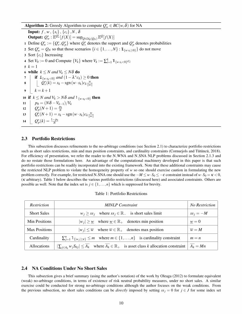
2.3 Portfolio RestrictionsThis subsection discusses refinements to the no-arbitrage conditions (see Section 2.1) to characterize portfolio restrictions

such as short sales restrictions, min and max position constraints, and cardinality constraints (Cornuejols and Tutuncu, 2018).For efficiency of presentation, we refer the reader to the N WNA and N SNA NLP problems discussed in Section 2.1.3 anddo no restate those formulations here. An advantage of the computational machinery developed in this paper is that suchportfolio restrictions can be readily incorporated into the existing framework. Note that these additional constraints may causethe restricted NLP problem to violate the homogeneity property of w so one should exercise caution in formulating the newproblem correctly. For example, for restricted N SNA one should use the−M≤w ·S0 ≤−ε constraint instead of w ·S0 = κ < 0,(κ arbitrary). Table 1 below describes the various portfolio restrictions (discussed here) and associated constraints. Others arepossible as well. Note that the index set is j ∈ 1, . . . ,n which is suppressed for brevity.

Table 1: Portfolio Restrictions

Restriction MINLP Constraint No Restriction

Short Sales w j ≥ ss j where ss j ∈ R− is short sales limit ss j =−M

Min Positions |w j| ≥ w where w ∈ R+ denotes min position w = 0

Max Positions |w j| ≤ w where w ∈ R+ denotes max position w = M

Cardinality ∑nj=11|w j|≥ε ≤ m where m ∈ 1, . . . ,n is cardinality constraint m = n

Allocations |∑ j∈Akw jS0 j| ≤ Ak where Ak ∈ R+ is asset class k allocation constraint Ak = Mn

2.4 NA Conditions Under No Short SalesThis subsection gives a brief summary (using the author’s notation) of the work by Oleaga (2012) to formulate equivalent

(weak) no-arbitrage conditions, in terms of existence of risk neutral probability measures, under no short sales. A similarexercise could be conducted for strong no-arbitrage conditions although the author focuses on the weak conditions. Fromthe previous subsection, no short sales conditions can be directly imposed by setting ss j = 0 for j ∈ J for some index set

10

J ⊆ 1, . . . ,n. Oleaga begins his paper with a remark that the Fundamental Theorem of Finance establishes the equivalencebetween the no-arbitrage conditions and the existence of a risk neutral probability measure (see Section 1.1 of this paper fordetails) under the assumption that short selling of risky securities is allowed. He remarks that when short sales are not allowed,the academic literature is scarce regarding equivalent conditions on probability measures. As motivation for his main result(which implies that existence of a risk neutral measure is not guaranteed under no short sales) the author develops two examples:one using a simple one-period binomial model with one risky asset, and another involving wagers in a stylized market where theassets are Arrow-Debreu securities. Using standard techniques in linear algebra, convex analysis, and the separating hyperplanetheorem the author proves his main result which is stated below for convenience.

Theorem. (Arbitrage Theorem for No Short Sales). The market modelM with m scenarios for n assets X j : j ∈ 1, . . . ,n hasno-arbitrage opportunities iff there exists a probability measure π such that the initial prices x j are greater than or equal to thediscounted value of the expected future prices under π . Written in symbols we have:

x j ≥1

1+ r0

m

∑i=1

πiXi j where j ∈ 1, . . . ,n.

Moreover, for those assets X j : j ∈ 1, . . . ,n where short selling is allowed, equality is achieved in the above relation. Inparticular, the bank account or cash bond (used to execute the borrowing to purchase the portfolio at time 0) is treated as aspecial asset X0 excluded from the above relation. It would hold with equality if included.

In an independent work, LeRoy and Werner (2014) develop essentially the same results for both weak and strong no-arbitrageconditions. They show that for the weak conditions, the probability measure π is such that π > 0 whereas for the strongconditions π ≥ 0.

2.5 Nearest NA ProblemRecall that the motivating question here is how to find the nearest arbitrage-free measure to the arbitrage admissible refer-

ence measure.

2.5.1 Short Sales Allowed

This subsection looks at the problem of computing the minimal distance δ ∗g to an arbitrage-free measure for a referencemeasure QN that admits arbitrage. In a discrete setting, the nearest (strong) no-arbitrage problem can be formulated as

δ∗ns = min

X‖X− X‖F such that ∃ q≥ 0 : p = Xq (NSP)

where ‖X‖F denotes the Frobenius norm of matrix X . A penalty relaxation can be formulated as

δ∗nsr(β ) = min

X ,q≥0‖X− X‖F +β‖p− Xq‖2

F (NSPR)

A tight lower bound δ ∗nst ≤ δ ∗ns to the relaxation problem NSPR is given by

δ∗nst = sup

β≥0δ∗nsr(β ) (NSPRT)

For a complete market with non-redundant securities, note that X (and hence X) is a full rank, invertible square n×n matrix.

2.5.2 No Short Sales

This subsection mimics the approach of the previous subsection, however we make use of the equivalent probability mea-sure condition discussed in Section 2.4 (Oleaga, 2012), (LeRoy and Werner, 2014). In a discrete setting, the nearest (weak)no-arbitrage problem, under no short sales, can be formulated as

δ∗nns = min

X‖X− X‖F such that ∃ probability measure q > 0 : p≥ X

1+ r0q. (NNWP)

A penalty relaxation can be specified as

δ∗nnsr(β ) = min

X ,q>0‖X− X‖F +β‖(Xq− (1+ r0)p)+‖2

F (NNWPR)

11

A tight lower bound δ ∗nnst ≤ δ ∗nns to the relaxation problem NNWPR is given by

δ∗nnst = sup

β≥0δ∗nnsr(β ) (NNWPRT)

Recall the bank account or cash bond (used to borrow) is excluded from the above relation. For a complete market withnon-redundant securities, note that X (and hence X) is a full rank, invertible square n×n matrix.

2.6 Alternate Robust NA ConditionsFor completeness, we comment on an alternate formulation of the robust NA conditions (from Section 2.1) that exchanges

the order of sup operators. Such conditions can be expressed as

supQ∈Uδ (QN)

supw∈Γs

EQ[1w·S1≥0 ]< 1 (RSNAP)

where Γs is defined in SW. The intuitive meaning of this formulation is that the market player first chooses a favorable distri-bution Q ∈ Uδ (QN) and then the portfolio manager chooses an optimal w ∈ Γs. It is clear that

supQ∈Uδ (QN)

supw∈Γs

EQ[1w·S1≥0 ] = supw∈Γs

supQ∈Uδ (QN)

EQ[1w·S1≥0 ].

3 Theory: Robust Statistical Arbitrage (SA) Conditions for Financial MarketsThis section develops the theory for robust statistical arbitrage in financial markets. We follow the same approach as in

Section 2 for robust arbitrage. For simplicity, and to ease the notation, let us focus on the strong conditions. The weak conditionscan be handled similarly, replacing w ∈ Γs with w ∈ Γw, as in Section 2. In Section 3.1, the primal problem for the SA best caseconditions is formulated using notions of statistical arbitrage as discussed in Section 1.4.3. The dual problem is formulatedusing the Lagrangian duality result from Section 1.4.4. The dual problem is a maximin stochastic optimization problem. Section3.2 touches on the best case SA distribution. In Section 3.3, the primal problem for the SA worst case conditions is formulated.The dual problem for this is maximax. Both dual problems can be solved as in Section 2. Section 3.4 touches on the worstcase SA distribution. Section 3.5 addresses portfolio restrictions. Section 3.6 covers the nearest SA problem. Section 3.7discusses alternate robust SA conditions. Altogether, this machinery gives us a practical approach to explore applications ofour framework in Sections 4 and 6.

3.1 Robust SA Best Case ConditionsThe robust (strong) statistical arbitrage best case conditions (of level αbc ∈ (0,1)) can be expressed as

supw∈Γs

supQ∈Uδ (QN)

EQ[1w·S1≥0 ]≤ αbc, (SSAP)

where Γs is defined in SW. As before, the indicator function 1w·S1≥0 on closed set w ·S1 ≥ 0 is upper semicontinuous hencewe can apply the duality theorem (see Section 1.4.4) to obtain the dual formulation

supw∈Γs

infλ≥0

[λδ +1N

N

∑i=1

Ψλ ,w(si) ]≤ αbc (SSAD)

where Ψλ ,w is defined, in terms of cost function c, as Ψλ ,w = sups∈Rn [1w·s≥0−λc(s,si) ].

3.1.1 Inner Optimization Problem

The goal here is the same as for the robust no-arbitrage conditions in Section 2.1.1, namely to evaluate Ψλ ,w in closed form.As such the solution is also the same, therefore one can invoke Proposition 2.1 to compute 1

N ∑Ni=1 Ψλ ,w(si).

3.1.2 Middle Optimization Problem

As before, in Section 2.1.2, the objective is to evaluate infλ≥0 H(λ ) := [λδ +K0(w)+K1(λ ,w) ]. As such the solution isalso the same, therefore one can invoke Propositions 2.2, 2.3 and Algorithm 1 to compute λ ∗ and H(λ ∗).

12

3.1.3 Outer Optimization Problem

As before, in Section 2.1.3, the objective is to evaluate vs(δ ) := supw∈Γsλ ∗(w,δ )δ +K0(w)+K1(λ

∗(w,δ ),w). As suchthe solution is also the same, therefore one can invoke Theorem 2.1 and Corollary 2.1.1 to evaluate the above expression(s).The analog to Theorem 2.2 is given below.

Theorem 3. The critical radius δ bcα can be expressed as infδ ≥ 0 : vs(δ )≥ αbc. Furthermore, δ bc

α can be explicitly computedvia binary search. Let δ < δ bc

α . For Q ∈ Uδ (QN), it follows that Q is (strong) statistical arbitrage free, for level α > vs(δbcα ).

For Q /∈ Uδ bc

α(QN), it follows that Q may admit (strong) statistical arbitrage for level α > vs(δ

bcα ).

Proof. This characterization of the critical radius δ bcα follows from the condition SSAD as well as the definition of (strong)

statistical arbitrage. The asymptotic properties of vs are such that vs(0)≤ 1 and limδ→∞ vs(δ ) = 1. Furthermore, since vs(δ ) isa non-decreasing function of δ , it follows that δ bc

α can be computed via binary search.

One can view critical radius δ bcα as a relative measure of the degree of (strong) statistical arbitrage in reference measure QN .

Those QN which are “close” to admitting statistical arbitrage of level αbc will have a relatively smaller value of δ bcα .

3.2 Best Case Distribution for SA ProblemThe characterization of best case distributions for NA problems carries over into the SA context. In particular, one is

interested in best case distributions Qαw ∈ BC(w,δ α) such that EQα

w [1w·S1≥0 ] = supQ∈Uδα (QN)EQ[1w·S1≥0 ]. As before, by

selecting portfolio weights wα that satisfy the outer sup condition

supw∈Γs

supQ∈Uδα (QN)

EQ[1w·S1≥0 ]≥ αbc,

one can recover Qαwα that admits statistical arbitrage of level αbc. See Section 6.2 for a concrete example.

3.3 Robust SA Worst Case ConditionsThe robust (strong) statistical arbitrage worst case conditions (of level αwc ∈ (0,1)) can be expressed as

supw∈Γs

infQ∈Uδ (QN)

EQ[1w·S1≥0 ]≥ αwc, (SSAPwc)

where Γs is defined in SW. Relaxing the objective function from 1w·S1≥0 to 1w·S1>0 and using the relations 1w·S1>0 =1−1w·S1≤0 and inf(S) =−sup(−S) for bounded set S, we have the equivalent condition:

supw∈Γs

−

sup

Q∈Uδ (QN)

EQ[1w·S1≤0−1 ]

≥ α

wc. (SSAP2wc)

As before, the indicator function 1w·S1≤0 on closed set w ·S1 ≤ 0 is upper semicontinuous hence we can apply the dualitytheorem (see Section 1.4.4) to obtain the dual formulation

supw∈Γs

−

infλ≥0

[λδ +1N

N

∑i=1

Ψwcλ ,w(si) ]

≥ α

wc (SSADwc)

where Ψwcλ ,w is defined, in terms of cost function c, as Ψwc

λ ,w = sups∈Rn [1w·s≤0−λc(s,si)−1 ].

3.3.1 Inner Optimization Problem

The goal here is the same as for the robust no-arbitrage conditions in Section 2.1.1, namely to evaluate Ψwcλ ,w in closed form.

There are two cases to consider.

Case 1.1w·si≤0 = 1 =⇒ Ψ

wcλ ,w(si) = 1− λ ·0 −1 = 0 which is optimal.

Case 2.1w·si≤0 = 0 =⇒ Ψ

wcλ ,w(si) = [1−λc(s∗i ,si)]

+−1 where s∗i = argmin‖s− si‖2 is optimal.

13

By the Projection Theorem (Calafiore and El Ghaoui, 2014), ‖s∗i − si‖2 =|w>si|‖w‖2

=⇒ Ψwcλ ,w(si) = [1−λci]

+−1 for

ci =|w>si|‖w‖2

∈ Rn+.

Proposition 4.1N

N

∑i=1

Ψwcλ ,w(si) = Kwc

0 (w)+Kwc1 (λ ,w) = Kwc

1 (λ ,w)

where Kwc0 (w) = 1

N ∑Ni=11w·si≤0 ·0 and Kwc

1 (λ ,w) = 1N ∑

Ni=11w·si>0([1−λci]

+−1) for ci =|w>si|‖w‖2

∈ Rn+.

Proof. This follows by a straightforward application of the two cases above.

3.3.2 Middle Optimization Problem

As before, in Section 2.1.2, the objective is to evaluate infλ≥0 Hwc(λ ) := [λδ +Kwc1 (λ ,w) ]. As such the solution is also

the same, with one exception: replace 1w·si<0 with 1w·si>0 in those results. Therefore one can apply Propositions 2.2, 2.3and Algorithm 1 (with the above replacement of indicator functions) to compute λ ∗ and Hwc(λ ∗).

3.3.3 Outer Optimization Problem

As before, in Section 2.1.3, the objective is to evaluate vwcs (δ ) := supw∈Γs

−λ ∗(w,δ )δ +Kwc1 (λ ∗(w,δ ),w). As such the

solution is similar, with the following adjustments: replace Fk(w) with −Fwck (w) where

−Fwck (w) := λkδ +

1N

[ N

∑i=1

(z+i −1)1w·si>0

]and place a minus sign in front of the min term in the maximin expression for vw(s)(δ ). Therefore one can apply Theorem 2.1and Corollary 2.1.1 (with the above adjustments) to evaluate vwc

s (δ ). The revised formulation is shown below.

Theorem 4. vwcs (δ ) is approximated by the (global) solution to nonlinear program (NLP) N SSA (listed below).

The constraints on variables below, with index i, apply for i ∈ 1, . . . ,N, although this is suppressed.

>

w∈Rn maximize<

b maxλk : k∈0,1,...,N

Fwck (w) =−λkδ +

1N

[ N

∑i=1

(1− z+i )1w·si>0

]vwc

s (δ ) =

subject to ci =|w>si|‖w‖2

,

λk =1ck∀k ∈ 1, . . . ,N,

λ0 = 0,|wi| ≤M,

w ·S0 ≤−ε,

zi = [1−λkci]

(2)

Proof. The NLP formulation follows from the definition of vwcs and the fact that λ ∗ ∈ 1

ck: k ∈ 1, . . . ,N∪λ0 := 0.

The analog to Theorem 2.2 is given below.

Theorem 5. The critical radius δ wcα can be expressed as infδ ≥ 0 : vwc

s (δ ) ≤ αwc. Furthermore, δ wcα can be explicitly

computed via binary search. Let δ < δ wcα . For Q ∈ Uδ wc

α(QN), it follows that Q admits (strong) statistical arbitrage, for level

α ≥ vwcs (δ wc

α ). For Q /∈ Uδ wcα(QN), it follows that Q may not admit (strong) statistical arbitrage for level α < vwc

s (δ wcα ).

Proof. This characterization of the critical radius δ wcα follows from the condition (SSADwc) as well as the definition of (strong)

statistical arbitrage. The asymptotic properties of vwcs are such that vwc

s (0) > 0 and limδ→∞ vwcs (δ ) = 0. Furthermore, since

vwcs (δ ) is a non-increasing function of δ , it follows that δ wc

α can be computed via binary search.

One can view critical radius δ wcα as a relative measure of the degree of (strong) statistical arbitrage in reference measure QN .

Those QN which are “close” to not admitting statistical arbitrage of level αwc will have a relatively smaller value of δ wcα .

14

3.4 Worst Case Distribution for SA ProblemThe characterization of worst case distributions for NA problems carries over into the SA context. In particular, one is

interested in worst case distributions Qαw ∈WC(w,δ α) such that EQα

[1w·S1≥0 ] = infQ∈Uδα (QN)EQ[1w·S1≥0 ]. By selecting

portfolio weights w with their associated worst case distributions, it follows that

supw∈Γs

EQαw [1w·S1≥0 ]≤ α

wc.

Applying the greedy algorithm to 1w·S1<0 = 1−1w·S1≥0, one can recover Qαw that is the most punitive for w and admits

statistical arbitrage of level at most αwc for a given w ∈ Γs. See Section 6.2 for a concrete example.

3.5 Portfolio Restrictions, SA Under No Short SalesThe portfolio restrictions for NA problems apply in the SA context as well. We refer the reader to Section 2.3 and do not

duplicate the material here. The Farkas Lemma characterization of classical weak (strong) no arbitrage via the existence (anduniqueness for complete markets) of risk neutral measures does not yield any new relationships in the context of statisticalarbitrage under no short sales. As such, we do not establish any new results in this subsection. Note that the theorem givenin Section 2.4 still holds for probability measures Qα for α ∈ (0,1); in words, it holds for market models that admit statisticalarbitrage but not classical arbitrage.

3.6 Nearest SA ProblemAs above, the Farkas Lemma characterization does not yield any new relationships for the nearest no-arbitrage problem in

the context of statistical arbitrage. However, the nuances of how one uses the existing results in Section 2.5 (vs. Section 2.4)are different. In particular, one can apply those results for probability measures Qα for α = 1; in words, it holds for marketmodels that admit classical arbitrage.

3.7 Alternate Robust SA ConditionsThe concept of exchanging the order of the sup and inf operators for the robust NA conditions (see Section 2.6) can be

extended to cover SA. As before, exchanging the order of the operators gives the robust SA best case conditions

supQ∈Uδ (QN)

supw∈Γs

EQ[1w·S1≥0 ]≤ αbc. (RSSAPbc)

Similarly, an alternate formulation of the robust SA worst case conditions is

infQ∈Uδ (QN)

supw∈Γs

EQ[1w·S1≥0 ]≥ αwc. (RSSAPwc)

The intuitive meaning of these formulations is that the market adversary first chooses a punitive distribution Q ∈ Uδ (QN) andthen the portfolio manager chooses an optimal w∈ Γs. Although one can invoke the min-max inequality to establish the relation

infQ∈Uδ (QN)

supw∈Γs

EQ[1w·S1≥0 ]≥ supw∈Γs

infQ∈Uδ (QN)

EQ[1w·S1≥0 ],

finding a method to compute the LHS of RSSAPbc or RSSAPwc is not really achievable (to our knowledge) since the innerproblem is NP Hard (see Section 5 for a proof) and the outer problem is infinite dimensional.

4 ApplicationsSection 4 presents applications of the theory developed in Sections 2 and 3 to robust option pricing and robust portfolio

selection. In the latter we consider two examples: the classical Markowitz problem and a more modern view of risk using CVaR(as opposed to variance) as the measure of risk.

15

4.1 Robust Option PricingThis subsection is a refinement (simplification) of the result for robust pricing of European options given in Bartl et al.

(2017). For clarity, we adopt the notation and problem setup of Example 2.14 (Robust Call) (Bartl et al., 2017). The approachtaken there is to add an additional constraint on the probability measure µ to reside within Wasserstein radius δ of the ref-erence (arbitrage-free) measure µ0. For this example, let us assume µ0 is arbitrage-free, distance function dc is the secondorder Wasserstein distance with associated quadratic cost function c(x,y) = (x− y)2/2,M1(R) denotes the set of probabilitymeasures on R, and the penalty function is φ := ∞1(δ ,∞] with associated convex conjugate φ ∗(λ ) = λδ . The authors show thatthe robust call option with maturity T , strike k, on a single asset, satisfies the relation:

CALLrobust(k) = supµ∈M1(R):

∫R Sdµ=s

CALL(k)−φ(dc(µ0,µ)) = infβ∈R

infλ>0

λδ +CALL(k− (2β +1)/(2λ ))+β

2/(2λ )

(3)

where β denotes the Lagrange multiplier for the arbitrage-free probability measure constraint µ ∈M1(R) :∫R Sdµ = s, and

λ denotes the Lagrange multiplier for the Wasserstein distance constraint dc(µ0,µ)≤ δ . Here CALL(k) denotes the non-robustcall option price for strike k. Now let us assume that we have calculated the critical radius δ ∗w(s) for this problem (assume thereference measure µ0 is empirical) and we have chosen δ α < min(δ ∗w,δ

∗s ). Here δ α denotes the radius of a Wasserstein ball

of probability measures that allow statistical arbitrage (up to some level α < 1) but not classical arbitrage. It follows fromTheorem 2.2 that the arbitrage-free probability measure constraint is not needed, hence one can simply set β := 0 in the aboveformula 3 to reduce it to the simpler formula:

CALLrobust(k) = infλ>0

G(λ ) :=

λδα +CALL(k−1/(2λ ))

. (4)

Note that in formula 4 above, G(λ ) is convex in λ . Once again, following the approach in our earlier work (Singh and Zhang,2019), we can simplify further to arrive at the following result.

Proposition 5. Let λ ∗ = supλ≥0λ : δ α − 1N [∑i∈J+1 (λ ) 1/(2λ 2)]≤ 0= infλ≥0λ : δ α − 1

N [∑i∈J1(λ ) 1/(2λ 2)]≥ 0,where

J+1 (λ ) = i ∈ 1, . . . ,N : [1/(2λ )+ si− k]> 0, J1(λ ) = i ∈ 1, . . . ,N : [1/(2λ )+ si− k]≥ 0.

Proof sketch. This result follows from writing down the first order conditions for left and right derivatives for convex objectivefunction G(λ ). Inspection of the left and right derivatives for G(λ ) reveals that they will cross zero (as λ sweeps from 0 to∞) and hence the sup and inf operators will apply over non-empty sets. For each index i ∈ J+1 (J1) we pick up another 1/(2λ 2)term in the left (right) derivative. Search on λ (from the left or the right) until we find λ ∗ such that 0 ∈ ∂G(λ ∗).

Proof. The first order optimality condition says

δα − 1

N ∑i∈J+1 (λ )

1/(2λ2)≤ 0≤ δ

α − 1N ∑

i∈J1(λ )

1/(2λ2).

Note the LHS is an increasing function in λ . Hence one can write

λ∗ = sup

λ≥0λ : δ

α − 1N ∑

i∈J+1 (λ )

1/(2λ2)≤ 0.

Similarly the RHS is also an increasing function in λ . Equivalently, one can write

λ∗ = inf

λ≥0λ : δ

α − 1N ∑

i∈J1(λ )

1/(2λ2)≥ 0.

Corollary 5.1.CALLrobust(k) = G(λ ∗) :=

[λ∗δ

α +CALL(k−1/(2λ∗))]

where λ ∗ is given by Proposition 4.1 above.

Proof. This follows by direct substitution of λ ∗ from Proposition 4.1 into formula 4 above.

16

4.2 Robust Portfolio Selection

4.2.1 Robust Markowitz Portfolio Selection

This subsection is a refinement of the result(s) for robust Markowitz (mean variance) portfolio selection given in Blanchetet al. (2018). For clarity, we adopt the notation and problem setup of that paper. The convex primal problem is a distributionallyrobust Markowitz problem given by

minφ∈Fδ ,r(N)

maxP∈Uδ (PN)

φ>VarP(R)φ (5)

where φ ∈ Rd denotes the portfolio weight vector, R ∈ Rd denotes the random (gross) asset returns, PN denotes the empiricalmeasure, Uδ (PN) denotes the uncertainty set for probability measures, with associated cost function c(u,v) = ‖v−u‖2

q for q≥ 1,VarP(R) denotes the covariance matrix of returns under P, and Fδ ,r(N) = φ : φ>1 = 1 ; minP∈Uδ (PN)EP(φ

>R) ≥ r denotesthe feasible region for portfolios. Using Lagrangian duality techniques (similar to this paper) the authors show that this primalproblem is equivalent to the convex dual problem

minφ∈Fδ ,r(N)

(√φ>VarPN (R)φ +

√δ‖φ‖p

)2

(6)

in terms of optimal value and solution(s), with 1/p+1/q = 1. Following the approach in the previous subsection, let us assumethe reference measure PN is arbitrage-free and we have chosen δ α < min(δ ∗w,δ

∗s ). Again δ α denotes the radius of a Wasserstein

ball of probability measures that allow statistical arbitrage (up to some level α < 1) but not classical arbitrage. It follows fromTheorem 2.2 that the arbitrage-free probability measure constraint is not needed hence the arbitrage-free primal problem

minφ∈Fδα ,r(N)

maxP∈Uδα (PN)

φ>VarP(R)φ (7)

where Uδ α (PN) = Uδ α (PN)∩P : supφ∈Γw∪Γs EP[1φ ·ST≥0 ] < 1 is equivalent to the primal and dual problems above. In

this setting R = R(S0,ST ) is the random vector of asset returns calculated based on initial asset prices S0 ∈ Rd and terminalasset prices ST ∈ Rd .

4.2.2 Robust Mean Risk Portfolio Selection

This subsection is a refinement of the result(s) for robust mean risk portfolio optimization given in Esfahani and Kuhn(2018). For clarity, we adopt the notation and problem setup of that paper. Let ξ ∈ Rm denote a random vector of (gross) assetreturns and x ∈X denote a vector of portfolio percentage weights ranging over the probability simplex X= x ∈Rm

+ : ∑mi=1 xi =

1. Thus we consider a “long only” portfolio. However, the reader is advised that today’s market includes securities such asexchange traded funds (ETFs) that behave like short positions hence the long portfolio setting is not as restrictive as it mightseem at first glance. The portfolio return is given by 〈x,ξ 〉. A single stage stochastic program which minimizes a weighted sumof the mean and CVaR of portfolio loss at confidence level α ∈ (0,1], given the investor’s risk aversion ρ ∈R+ and distributionP is given by

J∗ = infx∈XEP[−〈x,ξ 〉+ρ CVaRα(−〈x,ξ 〉)]. (8)

Substituting the formal definition of CVaR into the above, they show that

J∗ = infx∈XEP[−〈x,ξ 〉]+ρ inf

τ∈REP[τ +(1/α) max(−〈x,ξ 〉− τ,0)] (9)

= infx∈X,τ∈R

EP[maxk≤K

ak〈x,ξ 〉+bkτ] (10)

where K = 2, a1 =−1, a2 =−1− (ρ/α), b1 = ρ, b2 = ρ(1− (1/α)).For Wasserstein ambiguity set Bε(PN) of radius ε about reference measure PN , the authors formulate the distributionally

robust primal problemJN(ε) := inf

x∈Xsup

Q∈Bε (PN)

EQ[−〈x,ξ 〉+ρ CVaRα(−〈x,ξ 〉)] (11)

Applying techniques of Lagrangian duality, Esfahani and Kuhn formulate the equivalent dual problem

JN(ε) =

infx,τ,λ ,si,γik

λε + 1N ∑

Ni=1 si

such that x ∈ X,bkτ +ak〈x, ξi〉+ 〈γik,d−Cξi〉 ≤ si,

‖C>γik−akx‖∗ ≤ λ ,

γik ≥ 0

(12)

17

∀i ≤ N,∀k ≤ K. Following the approach in the previous subsection, let us assume the reference measure PN is arbitrage-freeand we have chosen εα < min(ε∗w,ε

∗s ). As before εα denotes the radius of a Wasserstein ball of probability measures that allow

statistical arbitrage (up to some level α < 1) but not classical arbitrage. It follows from Theorem 2.2 that the arbitrage-freeprobability measure constraint is not needed hence the arbitrage-free primal problem

infx∈X

supQ∈Bεα (PN)

EQ[−〈x,ξ 〉+ρ CVaRα(−〈x,ξ 〉)] (13)

where Bεα (PN) = Bεα (PN)∩Q : supφ(x)∈Γw∪Γs EQ[1φ(x)·ST≥0 ]< 1 is equivalent to the primal and dual problems above.

In this setting, ξ = ξ (S0,ST ) is the random vector of asset returns calculated based on initial asset prices S0 ∈ Rm and terminalasset prices ST ∈ Rm. Also, S0 = (S0,B0) appends the initial cash bond (borrowing) B0 used to purchase the portfolio (at zeroor negative cost) and ST = (ST ,BT ) appends the bond repayment (principal plus interest) at the end of the investment period.Finally, φ(x) ∈ Rm+1 for x ∈ X denotes the portfolio weight vector corresponding to the portfolio purchase and cash loan. Byconstruction, the first m components of φ are non-negative whereas the last component has a negative sign.

5 Complexity of NA ProblemThis section gives formal proofs for the complexity of the No-Arbitrage Problem. We establish that the weak and strong

no-arbitrage problems are NP Hard. The approach taken here is to use reduction on the known NP complete closed (open)hemisphere decision problem (Johnson and Preparata, 1978). The optimization problem, using the notation of this paper, isstated below (Avis et al., 2005).

1. closed hemisphere:Find w ∈ Rn such that card(i : si ∈ S; w · si ≥ 0) is maximized.

2. open hemisphere:Find w ∈ Rn such that card(i : si ∈ S; w · si > 0) is maximized.

To complete the problem statement, note that the set S above denotes a finite subset ofQn containing N points. It followsthat the mixed hemisphere problem (where ci ≥ 0 ∀i) is also NP complete.

3. mixed hemisphere:

supw∈Rn

[ N

∑i=1

1w·si≥0+N

∑i=1

ci1w·si<0]. (M1)

One can write a simplified version of the weak and strong no-arbitrage optimization problems as follows (see Section 2.1.3).To construct these simplified versions, we have fixed λ ∗ to a constant, relabeled [1−λci]

+ as ci, and omitted the initial costconstraint w ·S0 = κ . Recall κ is zero in the weak case, but strictly less than zero (for arbitrary κ) in the strong case.

supw∈Rn

F(w) :=[ N

∑i=1

1w·si≥0+N

∑i=1

ci1w·si<0]. (WD3,SD3)

However, there is some work to be done to incorporate the initial cost constraint back to formulate the no-arbitrage problems.First, think of the unconstrained initial cost as the union of three possibilities: (i) w ·S0 < 0, (ii) w ·S0 = 0, (iii) w ·S0 > 0. Somethought suggests that the following proposition holds.

Proposition 6. Asumming P 6= NP, there can be no polynomial time algorithm to solve the simplified no-arbitrage problemunder initial cost constraint w ·S0 ≤ κ for κ ∈ R.

Proof. Proceed by contradiction. Suppose there is a polynomial time algorithm A that can solve the following problem:

supw∈Rn,w·S0≤κ

F(w). (M2)

Exploiting symmetry, one can then also use algorithm A to solve this problem:

supw∈Rn,w·S0≥κ

F(w). (M3)

Returning the better answer now gives us a polynomial time algorithm to solve the mixed hemisphere problem which contradictsP 6= NP. Hence it must be that there is no polynomial time algorithm A to solve either M2 or M3.

18

Corollary 6.1. Asumming P 6= NP, there can be no polynomial time algorithms to solve both the weak and strong no-arbitrageproblems.

Proof. This follows directly from the definitions of the weak and strong no-arbitrage conditions (see Section 1.3.1).

Corollary 6.2. Asumming P 6= NP, there can be no polynomial time algorithms to solve either the weak or strong no-arbitrageproblems.

Proof. Recall that weight vectors w satisfy the homogeneity property. Hence the optimal solution to the strong no-arbitrageproblem is invariant to the actual choice of κ up to the sign. In other words, we have the following relation:

supw∈Rn,w·S0<0

F(w) = supw∈Rn,w·S0=κ<0(κ arbitrary)

F(w). (M4)

Furthermore, the RHS formulation above is equivalent in form to the weak no-arbitrage problem.

6 Computational StudyThis computational study uses the Matlab fminimax and fmincon solvers to work out a couple of concrete examples to find

the critical radii at the cusp of (statistical) arbitrage assuming short sales are allowed. Best (worst) case distributions and optimalportfolios are computed as well. Suitable values (for the problem instances below) for M range from 100 to 10,000 and for ε

from 0.001 to 0.0001. Other choices may be suitable. Recall that Matlab fminimax solves to local optimality using a sequentialquadratic programming (SQP) method with modifications (Fletcher, 2010). Similarly, fmincon solves to local optimality usinggradient based techniques. Our algorithm incorporates a few additional features to improve the robustness of the approach.These are listed next.

1. multi search: multiple search paths (that evolve candidate solutions) are used, similar to a genetic algorithm.

2. hot start: the optimal portfolio from the previous run δprev becomes the initial portfolio for the next run δnext .

3. function smoothing: the indicator function can be relaxed using a sigmoid with appropriate scale factor.

As mentioned in Section 2, developing an approach to solve for global optimality would be a topic for further research. Mean-while, for this section, the computed values for vw(s) and corresponding critical values for δ ∗w(s) represent local optimality (upper

bounds for globally optimal δ ∗w(s)). This comment also applies for the statistical arbitrage calculations for δ bcα and δ wc

α .

6.1 Binomial Tree Asset PricingFor the first example, consider the simple setting of a one-period binomial tree asset pricing model. There is a riskless bond

priced at par at time zero that earns a deterministic risk free rate of return r at time 1. In addition there is a risky asset (stock)with initial price s0 and time 1 price su = us0 that occurs with probability p= 1/2 and price sd = ds0 that occurs with probabilityq = 1− p = 1/2. The (weak) no-arbitrage conditions can be stated as: 0 < d < 1+ r < u (Shreve, 2005). Let us mock up anexample to satisfy these conditions. Consider the problem setting below. Here 0 < d = 0.966... < 1+ r ∈ 0.995,1.005< u =1.0333... thus the conditions are satisfied. Intuitively the investor could either make or lose money depending on what happens.

Solving NLP N WNA (see Theorem 2.1) for various values of δ gives the results in Table 2 (including the optimal port-folios). The critical radius δ ∗w from Theorem 2.2 is at most 1.5. Solving NLP N SNA (see Corollary 2.1.1) for various valuesof δ gives the results in Table 3. The critical radius δ ∗s is at most 1.5 as well. For this problem setup it appears that weak andstrong arbitrage occur together. A plot of these values (from both tables) is shown in Figure 2 below.

Table 2: vw(δ )< 1: Weak No-Arbitrage Condition

δ 0.001 0.1 0.25 0.5 1.0 1.25 1.5vw 0.50 0.54 0.59 0.69 0.87 0.97 1.0

wstock 1.3 -0.7 -0.7 -0.7 -0.7 -0.7 -0.5wbond -3.9 2.1 2.1 2.1 2.1 2.1 1.5

19

Figure 1: One-Period Binomial Tree

Stock =$310Bond =$100.5

Stock = $300Bond = $100

Stock =$290Bond =$99.5

p

q =(1− p)

Table 3: vs(δ )< 1: Strong No-Arbitrage Condition

δ 0.001 0.1 0.25 0.50 1.0 1.25 1.5vs 0.50 0.54 0.59 0.69 0.87 0.97 1.0

wstock 1.3 188 188 188 -300 -300 -82wbond -3.9 -565 -565 -565 899 899 247

Figure 2: Arbitrage Probabilities for One-Period Binomial Asset Pricing

0 0.5 1 1.5

0.4

0.6

0.8

1

1.2

Delta

Prob

abili

ty

0.4

0.6

0.8

1

1.2

Prob

abili

ty

StrongWeak

6.2 Pairs TradingA typical example of a pairs trade would be to trade a linear combination of cointegrated tickers. The idea is to exploit

temporary divergence from the long run relationship in the belief that convergence to the long run mean will result in a profitabletrading strategy (Wojcik, 2005). The following annual data set of month end closing prices is taken from Yahoo finance website.A plot of this market data is shown in Figure 3 below.

20

Table 4: U.S. Tech Pair Market Data 2019

Date 04/01 05/01 06/01 07/01 08/01 09/01Google 1,188.48 1,103.63 1,080.91 1,216.68 1,188.10 1,219.00Amazon 1,926.52 1,775.07 1,893.63 1,866.78 1,776.29 1,735.91

Table 5: U.S. Tech Pair Market Data 2019/2020

Date 10/01 11/01 12/01 01/01 02/01 03/01Google 1,260.11 1,304.96 1,337.02 1,434.23 1,339.33 1,298.41Amazon 1,776.66 1,800.80 1,847.84 2,008.72 1,883.75 1,901.09

Figure 3: U.S. Tech Pair Market Data

0 2 4 6 8 10 121,000

1,100

1,200

1,300

1,400

1,500

Month

Clo

sing

Pric

es

0 2 4 6 8 10 121,700

1,800

1,900

2,000

2,100

2,200

Month

Clo

sing

Pric

es

AmazonGoogle

Solving NLP N SNA for various values of δ gives the results in Table 6. A plot of these values is shown in Figure 4 below.The entire 12 point data set is used as the support for the time 1 distribution. The arithmetic average is used for the time 0prices. The data tuples of closing prices are assigned to the (uniform) discrete distribution for time 1.

Table 6: vs(δ ): SA Best Case

δ 0.001 1 2 5 10 20 31 31.7vs 0.58 0.67 0.69 0.77 0.83 0.93 0.99 1.0

wgoogle 10.1 100.0 100.0 100.0 100.0 100.0 100.0 100.0wamazon -6.9 -67.5 -67.5 -67.5 -67.5 -67.5 -67.5 -67.5

A plot of the best case (bc) distribution is shown in Figure 5 below. Recall the robust (strong) no-arbitrage conditions are

supw∈Γw(s)

supQ∈Uδ (QN)

EQ[1w·S1≥0 ]< 1.

The best case distribution has the property that the inner sup evaluates to 1 for δ ≥ δ ∗ = 31.7 (critical radius from Table 6above). Using the optimal portfolio w∗ = 100.0,−67.5 from Table 6, corresponding to δ = δ ∗, the outer sup also evaluates

21

Figure 4: Arbitrage Probabilities for U.S. Tech Pair

0 10 20 30

0.4

0.6

0.8

1

1.2

Delta

Prob

abili

ty

Best Case

to 1. Using the greedy algorithm discussed in Section 2.2 one recovers an arbitrage distribution. From the plot in Figure 5 it isclear that Google dominates Amazon which allows for the profit making opportunity.

Also from Table 6 one case see that for α = 0.99 the critical radius is δ bcα = 31. It turns out that point 3 is the most expensive

to move towards the arbitrage conditions, as Amazon dominates Google here (instead of the other way around). Moving 95% ofits mass towards the new values (and using the arbitrage admissible distribution for the remaining points) recovers the statisticalarbitrage distribution for α = 0.99. See Table 7 for the detailed probability mass function (PMF) for α = 0.99. Recall that onepoint mass from the reference distribution can be split into two pieces according to the budget constraint δ . In this case, thishappens for point 3. 95% of its mass is moved towards the new values in point 13.

Figure 5: U.S. Tech Pair Best Case Distribution

0 2 4 6 8 10 121,100

1,200

1,300

1,400

1,500

Month

Clo

sing

Pric

es

0 2 4 6 8 10 121,700

1,800

1,900

2,000

2,100

Month

Clo

sing

Pric

es

AmazonGoogle

22

Table 7: Best Case PMF for α = 0.99

Point 1 2 3 4 5 6 7 8 9 10 11 12 13Prob 1/12 1/12 0.0041 1/12 1/12 1/12 1/12 1/12 1/12 1/12 1/12 1/12 0.0792

Google 1,265 1,169 1,081 1,247 1,196 1,219 1,260 1,305 1,337 1,434 1,339 1,298 1,217Amazon 1,875 1,731 1,894 1,847 1,771 1,736 1,777 1,801 1,848 2,009 1,884 1,901 1,802

Switching to the worst case SA conditions, solving NLP N SSA for various values of δ gives the results in Table 8. A plotof these values is shown in Figure 6 below. The problem setup is the same as for the best case SA conditions above. A plot of theworst case (wc) distribution Qα

wα for α = 0 is shown in Figure 7 below. The corresponding portfolio is wα = 99.11,−66.864.These results were calculated using the Matlab fmincon solver, aplpying a grid search over λ to solve the maximax problem(which is convex in λ ). Using the greedy algorithm discussed in Section 2.2 one recovers a no-win distribution. From theplot in Figure 7 it is clear that neither Amazon nor Google dominates at all points but for the optimal portfolio wα , a quickcheck verifies that this distribution leads to a no-win situation, meaning EQα

wα [1wα ·S1≥0 ] = 0. Our calculations show that forα = 0 the critical radius is δ wc

α = 31.4. See Table 9 for the detailed probability mass function (PMF). Finally, Figure 8 showsthe absolute values of these two positions in the optimal portfolio with weights wα . Here the dominance of the short Amazonposition is easier to see.

Table 8: vwcs (δ ): SA Worst Case

δ 0.001 1 2 5 10 20 31 31.4vwc

s 0.58 0.51 0.47 0.41 0.31 0.11 0.004 0.0wgoogle 2.94 99.97 98.55 99.08 99.08 99.36 99.36 2.94

wamazon -1.98 -67.44 -67.48 -66.84 -66.84 -67.02 -67.02 -1.98

Figure 6: Arbitrage Probabilities for U.S. Tech Pair

0 10 20 300

0.2

0.4

0.6

0.8

1

Delta

Prob

abili

ty

Worst Case

23

Figure 7: U.S. Tech Pair Worst Case Distribution

0 2 4 6 8 10 121,000

1,100

1,200

1,300

1,400

Month

Clo

sing

Pric

es

0 2 4 6 8 10 121,700

1,800

1,900

2,000

2,100

Month

Clo

sing

Pric

es

AmazonGoogle

Table 9: Worst Case PMF for α = 0

Point 1 2 3 4 5 6 7 8 9 10 11 12Prob 1/12 1/12 1/12 1/12 1/12 1/12 1/12 1/12 1/12 1/12 1/12 1/12

Google 1,188 1,104 1,081 1,217 1,188 1,186 1,218 1,243 1,275 1,380 1,292 1,288Amazon 1,927 1,775 1,894 1,867 1,776 1,758 1,805 1,843 1,890 2,045 1,916 1,908

Figure 8: U.S. Tech Pair Worst Case Positions: Absolute Values

0 2 4 6 8 10 121

1.1

1.2

1.3

1.4·105

Month

Port

folio

Posi

tions

0 2 4 6 8 10 121

1.1

1.2

1.3

1.4·105

Month

Port

folio

Posi

tions

AmazonGoogle

24

6.3 Basket TradingBasket trading involves simultaneous trading of a basket of stocks. This example computes the critical radius for a small

basket of U.S. equities from the S&P 500 index used in the statistical arbitrage study by (Zhao et al., 2018). Table 10 belowlists the stock tickers, names, and industries. Table 11 displays a partial listing of the 5y historical market data set from March2015 through March 2020 used in this study. As before, the arithmetic average is used for time 0 and the data tuples for time1. Table 12 and Figure 9 display the optimal portfolios and best case arbitrage probabilities. Figures 10 and 11 show differentviews of the best case distribution for α = 1 and optimal portfolio wα = 17.20,−0.24,10.90,−11.19,−41.23,2.07,−3.90.The quantiles in Figure 11b are 0.25,0.5,0.75 respectively.

Table 10: Basket Constituents

Ticker Name Industry Market Cap (bn)APA Apache Corporation Energy: Oil and Gas 10.68AXP American Express Company Credit Services 109.0CAT Caterpillar Inc. Farm Machinery 74.94COF Capital One Financial Corp. Credit Services 46.19FCX Freeport-McMoRan Inc. Copper 17.33IBM 1nternational Business Machines Corp. Technology 132.70

MMM 3M Company Industrial Machinery 90.33

Table 11: Basket 2019 Market Data

Date 06/01 07/01 08/01 09/01 10/01 11/01 12/01APA 28.13 23.71 21.17 25.12 21.25 22.11 25.39AXP 122.16 123.08 119.50 117.42 116.43 119.71 124.06CAT 133.26 128.74 117.25 124.45 135.77 143.72 146.65COF 89.62 91.28 85.56 90.26 92.51 99.22 102.51FCX 11.45 10.91 9.10 9.48 9.73 11.34 13.07IBM 133.31 143.31 131.02 142.24 130.80 131.51 132.65

MMM 168.77 170.11 157.45 161.53 162.11 166.80 174.84

Table 12: vs(δ ): SA Best Case

δ 0.001 0.01 0.05 0.1 0.5 1vs 0.67 0.71 0.75 0.81 0.95 1.0

wapa 5.31 16.37 7.03 -7.61 6.38 17.2waxp -3.90 -7.50 -6.44 -14.45 -4.75 -0.24wcat -3.03 2.69 -0.94 5.54 6.36 10.90wco f 5.29 -11.00 -5.27 14.53 1.66 -11.19w f cx 9.59 -7.39 17.31 -92.13 -52.97 -41.23wibm -7.12 -6.56 -5.83 3.00 0.68 2.07

wmmm 4.82 9.08 7.86 3.38 -0.41 -3.90

25

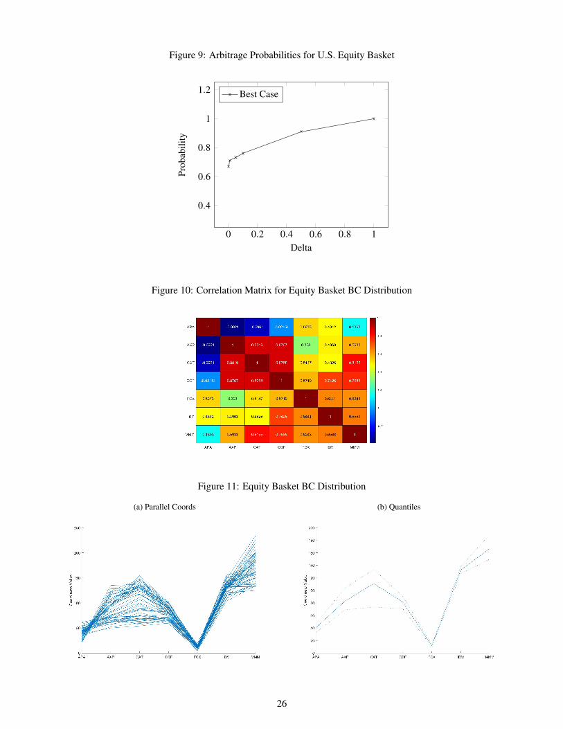
Figure 9: Arbitrage Probabilities for U.S. Equity Basket

0 0.2 0.4 0.6 0.8 1

0.4

0.6

0.8

1

1.2

Delta

Prob

abili

ty

Best Case

Figure 10: Correlation Matrix for Equity Basket BC Distribution

Figure 11: Equity Basket BC Distribution

(a) Parallel Coords (b) Quantiles

26

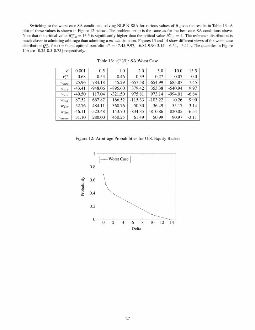
Switching to the worst case SA conditions, solving NLP N SSA for various values of δ gives the results in Table 13. Aplot of these values is shown in Figure 12 below. The problem setup is the same as for the best case SA conditions above.Note that the critical value δ wc

α=0 = 13.5 is significantly higher than the critical value δ bcα=1 = 1. The reference distribution is

much closer to admitting arbitrage than admitting a no-win situation. Figures 13 and 14 show different views of the worst casedistribution Qα

wα for α = 0 and optimal portfolio wα = 7.45,9.97,−6.84,9.90,3.14,−6.54,−3.11. The quantiles in Figure14b are 0.25,0.5,0.75 respectively.

Table 13: vwcs (δ ): SA Worst Case

δ 0.001 0.5 1.0 2.0 5.0 10.0 13.5vwc

s 0.68 0.53 0.46 0.39 0.27 0.07 0.0wapa 25.96 784.18 -45.29 -657.58 -654.99 685.87 7.45waxp -43.41 -948.06 –895.60 379.42 353.38 -540.94 9.97wcat -40.50 117.04 -321.50 975.81 973.14 -994.01 -6.84wco f 87.52 667.87 166.52 -115.33 -103.22 -0.26 9.90w f cx 52.76 484.11 360.76 -50.30 -36.49 55.17 3.14wibm -46.11 -523.48 143.70 -834.35 -810.86 820.05 -6.54

wmmm 31.10 280.00 450.25 61.49 50.99 90.97 -3.11

Figure 12: Arbitrage Probabilities for U.S. Equity Basket

0 2 4 6 8 10 12 140

0.2

0.4

0.6

0.8

1

Delta

Prob

abili

ty

Worst Case

27

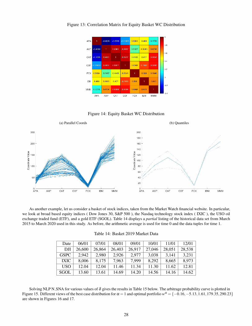
Figure 13: Correlation Matrix for Equity Basket WC Distribution

Figure 14: Equity Basket WC Distribution

(a) Parallel Coords (b) Quantiles

As another example, let us consider a basket of stock indices, taken from the Market Watch financial website. In particular,we look at broad based equity indices ( Dow Jones 30, S&P 500 ), the Nasdaq technology stock index ( IXIC ), the USO oilexchange traded fund (ETF), and a gold ETF (SGOL). Table 14 displays a partial listing of the historical data set from March2015 to March 2020 used in this study. As before, the arithmetic average is used for time 0 and the data tuples for time 1.

Table 14: Basket 2019 Market Data

Date 06/01 07/01 08/01 09/01 10/01 11/01 12/01DJI 26,600 26,864 26,403 26,917 27,046 28,051 28,538

GSPC 2,942 2,980 2,926 2,977 3,038 3,141 3,231IXIC 8,006 8,175 7,963 7,999 8,292 8,665 8,973USO 12.04 12.04 11.46 11.34 11.30 11.62 12.81

SGOL 13.60 13.61 14.69 14.20 14.56 14.16 14.62

Solving NLP N SNA for various values of δ gives the results in Table 15 below. The arbitrage probability curve is plotted inFigure 15. Different views of the best case distribution for α = 1 and optimal portfolio wα = −0.16,−5.13,1.61,179.35,290.23are shown in Figures 16 and 17.

28

Table 15: vs(δ ): SA Best Case

δ 0.001 0.01 0.05 0.1 0.5 0.6vs 0.68 0.68 0.70 0.81 0.99 1.0

wd ji 0.80 1.55 1.37 0.83 0.95 -0.16wgspc -0.04 -0.77 2.73 2.54 -11.65 -5.13wixic -2.70 -4.97 -5.45 -3.21 0.08 1.61wuso -6.01 4.42 105.07 21.27 -392.33 179.35wsgol -0.01 -17.15 -232.03 -334.96 1,000.00 290.23

Figure 15: Arbitrage Probabilities for Basket of Indices

0 0.1 0.2 0.3 0.4 0.5 0.6

0.4

0.6

0.8

1

1.2

Delta

Prob

abili

ty

Best Case

Figure 16: Correlation Matrix for Indices BC Distribution

29

Figure 17: Indices BC Distribution

(a) Parallel Coords (b) Quantiles

Switching to the worst case gives the results in Table 16 below. The arbitrage probability curve is plotted in Figure 18. Notethat the critical value δ wc

α=0 = 32.6 is significantly higher than the critical value δ bcα=1 = 0.6. As before, the reference distribution

is much closer to admitting arbitrage than admitting a no-win situation. Different views of the worst case distribution for α = 0and optimal portfolio wα = 1.84,8.42,−9.52,9.0,3.0 are shown in Figures 19 and 20.

Table 16: vwcs (δ ): SA Worst Case

δ 0.001 1.0 2.0 5.0 10.0 20.0 32.6vwc

s 0.68 0.64 0.61 0.55 0.45 0.25 0.0wd ji 110.62 184.78 142.34 49.08 189.16 260.27 1.84

wgspc -71.35 -83.14 -53.80 -18.59 -71.69 -98.82 8.42wixic -349.21 -597.31 -464.08 -160.00 -616.62 -848.45 -9.52wuso -55.20 29.16 16.30 5.79 14.07 46.47 9.00wsgol 19.75 -232.03 5.59 5.33 4.45 23.25 3.00

Figure 18: Arbitrage Probabilities for Basket of Indices

0 10 20 300

0.2

0.4

0.6

0.8

1

Delta

Prob

abili

ty

Worst Case

30

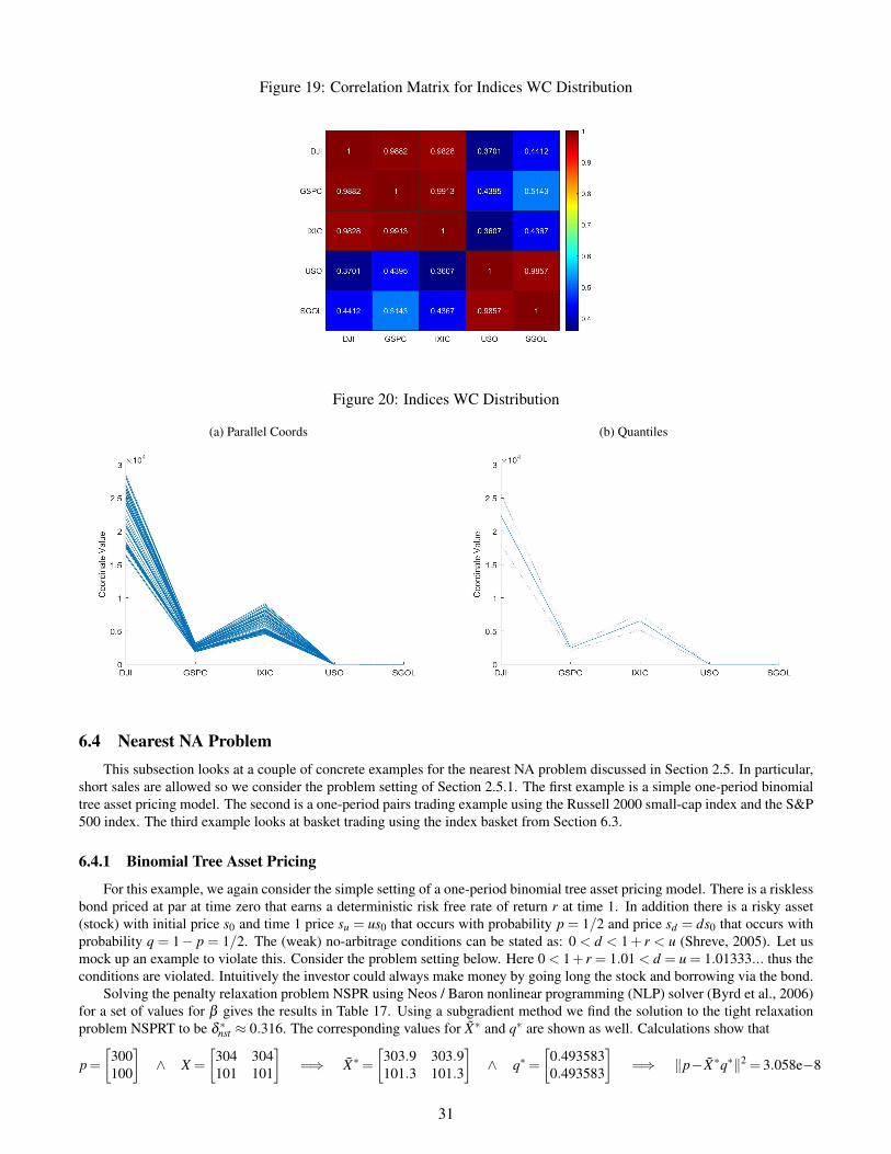
Figure 19: Correlation Matrix for Indices WC Distribution

Figure 20: Indices WC Distribution

(a) Parallel Coords (b) Quantiles

6.4 Nearest NA ProblemThis subsection looks at a couple of concrete examples for the nearest NA problem discussed in Section 2.5. In particular,

short sales are allowed so we consider the problem setting of Section 2.5.1. The first example is a simple one-period binomialtree asset pricing model. The second is a one-period pairs trading example using the Russell 2000 small-cap index and the S&P500 index. The third example looks at basket trading using the index basket from Section 6.3.

6.4.1 Binomial Tree Asset Pricing

For this example, we again consider the simple setting of a one-period binomial tree asset pricing model. There is a risklessbond priced at par at time zero that earns a deterministic risk free rate of return r at time 1. In addition there is a risky asset(stock) with initial price s0 and time 1 price su = us0 that occurs with probability p = 1/2 and price sd = ds0 that occurs withprobability q = 1− p = 1/2. The (weak) no-arbitrage conditions can be stated as: 0 < d < 1+ r < u (Shreve, 2005). Let usmock up an example to violate this. Consider the problem setting below. Here 0 < 1+ r = 1.01 < d = u = 1.01333... thus theconditions are violated. Intuitively the investor could always make money by going long the stock and borrowing via the bond.

Solving the penalty relaxation problem NSPR using Neos / Baron nonlinear programming (NLP) solver (Byrd et al., 2006)for a set of values for β gives the results in Table 17. Using a subgradient method we find the solution to the tight relaxationproblem NSPRT to be δ ∗nst ≈ 0.316. The corresponding values for X∗ and q∗ are shown as well. Calculations show that

p=[

300100

]∧ X =

[304 304101 101

]=⇒ X∗=

[303.9 303.9101.3 101.3

]∧ q∗=

[0.4935830.493583

]=⇒ ‖p−X∗q∗‖2 = 3.058e−8

31

Figure 21: One-Period Binomial Tree

Stock =$304Bond =$101

Stock = $300Bond = $100

Stock =$304Bond =$101

p

q =(1− p)

Table 17: Min Distance to Arbitrage-Free Measure

β 1 2 4 8 16 32 64 128 256 512 1024δ ∗nsr 0.098 0.188 0.252 0.284 0.300 0.308 0.312 0.314 0.315 0.316 0.316

For the complete markets problem, using the Neos / Knitro solver,

p=[

300100

]∧ X =

[304 304101 101

]=⇒ X∗=

[304.0 303.9101.0 101.3

]∧ q∗=

[0

0.987167

]=⇒ ‖p−X∗q∗‖2 = 8.786e−23

with minimal distance δ ∗cns ≈ 0.316. As another example (using the subgradient method) we find that

p=[

300100

]∧ X =

[309 306101 101

]=⇒ X∗=

[309 305.7

101.0 101.899

]∧ q∗=

[0

0.981354

]=⇒ ‖p−X∗q∗‖2 = 1.038e−8

with tight relaxation δ ∗nst ≈ 0.949. For the complete markets problem, we arrive at essentially the same solution.

6.4.2 Pairs Trading

This example uses the Russell 2000 and S&P 500 indices to conduct pairs trading on an annual data set of month end closingprices from the Yahoo website, as shown in Tables 18 and 19. A plot of this market data is shown in Figure 22. To satisfythe (strong) arbitrage conditions, an initial asset price vector S0 = 1,660,2,750 is selected. The portfolio w∗ = −1.0,0.6satisfies the (strong) arbitrage condition, for time 1 asset price vector S1 following a uniform discrete distribution with theannual data set as its support. Converting to the nearest NA problem setting of p = Xq, this support is used as the scenariomatrix X and the initial asset price vector S0 is used as the price vector p.

Table 18: Russell 2k and S&P 500 Market Data 2019

Date 04/01 05/01 06/01 07/01 08/01 09/01Russell 2k 1,591 1,466 1,567 1,577 1,495 1,523S&P 500 2,946 2,752 2,942 2,980 2,926 2,977

Solving the penalty relaxation problem NSPR using Neos / Knitro nonlinear programming (NLP) solver (Byrd et al., 2006)for a set of values for β gives the results in Table 20. Using a subgradient method we find the solution to the tight relaxationproblem NSPRT to be δ ∗nst ≈ 160.36. The corresponding values for X∗ and q∗ are shown as well.

32

Table 19: Russell 2k and S&P 500 Market Data 2019/2020

Date 10/01 11/01 12/01 01/01 02/01 03/01Russell 2k 1,562 1,625 1,668 1,614 1,476 1,153S&P 500 3,038 3,141 3,230 3,226 2,954 2,585

Figure 22: Russell 2k and S&P 500 Market Data

0 2 4 6 8 10 12

1,200

1,400

1,600

Month

Port

folio

Posi

tions

0 2 4 6 8 10 12

2,600

2,800

3,000

3,200

Month

Port

folio

Posi

tions

SP500Russell2k

Table 20: Min Distance to Arbitrage-Free Measure

β 1 2 4 8 16 32 64 128 256 512 1024δ ∗nsr 160.09 160.23 160.29 160.33 160.35 160.35 160.36 160.36 160.36 160.36 160.36

p=[

1,6602,750

]∧ X =

[1,591 1,466 1,567 1,577 1,495 1,523 1,562 1,625 1,668 1,614 1,476 1,1532,946 2,752 2,942 2,980 2,926 2,977 3,038 3,141 3,230 3,226 2,954 2,585

]=⇒

X∗ =[

1,728.29 1,466 1,567 1,577 1,495 1,523 1,562 1,625 1,668 1,614 1,476 1,1532,863.13 2,752 2,942 2,980 2,926 2,977 3,038 3,141 3,230 3,226 2,954 2,585

]∧

q∗ =[0.960488 0 0 0 0 0 0 0 0 0 0 0

]=⇒ ‖p− X∗q∗‖2 = 2.58e−7.

6.4.3 Basket Trading

This example uses the index basket from Section 6.3 to conduct trading. The reference data set is the 2019 month endclosing prices from the Yahoo website, as shown in Tables 21 and 22. A plot of this market data is shown in Figure 23. Tosatisfy the (strong) arbitrage conditions, an initial asset price vector S0 = 28256,3226,9151,10.84,15.27 is selected. Theportfolio w∗ = 0.16,5.13,−1.61,−179.35,−290.23 satisfies the (strong) arbitrage condition, for time 1 asset price vector S1following a uniform discrete distribution with the annual data set as its support. Converting to the nearest NA problem settingof p = Xq, this support is used as the scenario matrix X and the initial asset price vector S0 is used as the price vector p.

33

Table 21: Index Basket 2019 Market Data

Date 01/01 02/01 03/01 04/01 05/01 06/01DJI 25,000 25,916 25,929 26,593 24,815 26,600

GSPC 2,704 2,785 2,834 2,946 2,752 2,942IXIC 7,282 7,533 7,729 8,095 7,453 8,006USO 11.35 11.95 12.50 13.29 11.10 12.04

SGOL 12.73 12.65 12.46 12.37 12.59 13.60

Table 22: Index Basket 2019 Market Data

Date 07/01 08/01 09/01 10/01 11/01 12/01DJI 26,864 26,403 26,917 27,046 28,051 28,538

GSPC 2,980 2,926 2,977 3,038 3,141 3,231IXIC 8,175 7,963 7,999 8,292 8,665 8,973USO 12.04 11.46 11.34 11.30 11.62 12.81

SGOL 13.61 14.69 14.20 14.56 14.16 14.62

Figure 23: Indices Reference Distribution

(a) Parallel Coords (b) Quantiles

Solving the penalty relaxation problem NSPR using Neos / Knitro nonlinear programming (NLP) solver (Byrd et al., 2006)for a set of values for β gives the results in Table 23. Using a subgradient method we find the solution to the tight relaxationproblem NSPRT to be δ ∗nst ≈ 130.07. The corresponding values for X∗ and q∗ are shown as well.

Table 23: Min Distance to Arbitrage-Free Measure

β 1 2 4 8 16 32 64 128 256 512 1024δ ∗nsr 129.57 129.82 129.95 130.01 130.04 130.06 130.07 130.07 130.07 130.07 130.07

34

p =

25,000

2,7047,72912.5012.46

∧

X =

25,000 25,916 25,929 26,593 24,815 26,600 26,864 264,03 26,917 27,046 28,051 28,538

2,704 2,785 2,834 2,946 2,752 2,942 2,980 2,926 2,977 3,038 3,141 3,2307,282 7,533 7,729 8,095 7,453 8,006 8,175 7,963 7,999 8,292 8,665 8,97311.35 11.95 12.50 13.29 11.10 12.04 12.04 11.46 11.34 11.30 11.62 12.8112.73 12.65 12.46 12.37 12.59 13.60 13.61 14.69 14.20 14.56 14.16 14.62

=⇒

X∗=

25,000 25,918.88 25,929 26,593 24,815 26,600 26,864 264,03 26,917 27,046 28,051 28,546.396

2,704 2,743.19 2,834 2,946 2,752 2,942 2,980 2,926 2,977 3,038 3,141 3,108.2497,282 7,538.30 7,729 8,095 7,453 8,006 8,175 7,963 7,999 8,292 8,665 8,988.43511.35 12.51 12.50 13.29 11.10 12.04 12.04 11.46 11.34 11.30 11.62 14.42912.73 12.56 12.46 12.37 12.59 13.60 13.61 14.69 14.20 14.56 14.16 14.351

∧ q∗ =

[0 0.229248 0 0 0 0 0 0 0 0 0 0.667620

]=⇒ ‖p− X∗q∗‖2 = 4.78e−7.

7 Conclusions and Further WorkThis work has developed theoretical results and investigated calculations of robust arbitrage-free markets under distri-

butional uncertainty using Wasserstein distance as an ambiguity measure. The financial market overview and foundationalnotation and problem definitions were introduced in Section 1. Using recent duality results (Blanchet and Murthy, 2019), thesimpler dual formulation and its mixture of analytic and computational solutions were derived in Section 2. In Section 3 therobust arbitrage methodology was extended to encompass statistical arbitrage. In Section 4, some applications to robust optionpricing and portfolio selection were presented. Section 5 gave formal proofs for the NP Hardness of the NA problem. In Section6, we performed a computational study to calculate the critical radii (for the arbitrage conditions), optimal portfolios, and best(worst) case distributions for some concrete examples. The examples included a simple binomial tree, a pairs trading data set,and two trading baskets. The nearest NA problem was also explored to complete the study. Finally, we conclude with somecommentary on directions for further research.

One direction for future research, as has been previously discussed in Section 1.4.2, would be to investigate robust arbitrageproperties in a multi period continuous time setting for a suitable class of admissible trading strategies. Recall that a moregeneral version of the fundamental theorem of asset pricing applies there. Additional detail on this topic can be found inDelbaen and Schachermayer (2006). Another direction for future research, as mentioned in Section 2, would be to develop(and apply) a global solution strategy for the NLP problem formulations of Section 2.1.3. One possibility (as mentioned) isto construct an MINLP problem formulation, in programming languages such as GAMS, that is solvable to global optimalityusing the Baron solver, for example. Perhaps a third direction for future research would be to investigate notions of robust(modern) portfolio theory applying and/or extending the framework developed thus far.

Data Availability StatementThe raw and/or processed data required to reproduce the findings from this research can be obtained from the corresponding

author, [D.S.], upon reasonable request.

Conflict of Interest StatementThe authors declare they have no conflict of interest.

Funding StatementThe authors received no specific funding for this work.

35

ReferencesAndrei, N. and Andrei, N. (2013). Nonlinear optimization applications using the GAMS technology. Springer.

Avis, D., Hertz, A., and Marcotte, O. (2005). Graph theory and combinatorial optimization, volume 8. Springer Science &Business Media.

Bartl, D., Drapeau, S., and Tangpi, L. (2017). Computational aspects of robust optimized certainty equivalents and optionpricing.

Bartl, D. et al. (2019). Exponential utility maximization under model uncertainty for unbounded endowments. The Annals ofApplied Probability, 29(1):577–612.

Blanchet, J., Chen, L., and Zhou, X. Y. (2018). Distributionally robust mean-variance portfolio selection with wassersteindistances.

Blanchet, J., Kang, Y., and Murthy, K. (2016). Robust wasserstein profile inference and applications to machine learning. arXivpreprint arXiv:1610.05627.

Blanchet, J. and Murthy, K. (2019). Quantifying distributional model risk via optimal transport. Mathematics of OperationsResearch, 44(2):565–600.

Byrd, R., Nocedal, J., and KNITRO, R. W. (2006). An integrated package for nonlinear optimization.

Calafiore, G. C. and El Ghaoui, L. (2014). Optimization models. Cambridge university press.

Cornuejols, G. and Tutuncu, R. (2018). Optimization methods in finance. Cambridge University Press, 2 edition.

Delbaen, F. and Schachermayer, W. (2006). The mathematics of arbitrage. Springer Science & Business Media.

Dinh, N., Goberna, M. A., Lopez, M., and Mo, T. H. (2017). Robust optimization revisited via robust vector farkas lemmas.Optimization, 66(6):939–963.

Esfahani, P. M. and Kuhn, D. (2018). Data-driven distributionally robust optimization using the wasserstein metric: Perfor-mance guarantees and tractable reformulations. Mathematical Programming, 171(1-2):115–166.

Fletcher, R. (2010). The sequential quadratic programming method. In Nonlinear optimization, pages 165–214. Springer.

Focardi, S. M., Fabozzi, F. J., and Mitov, I. K. (2016). A new approach to statistical arbitrage: Strategies based on dynamicfactor models of prices and their performance. Journal of Banking & Finance, 65:134–155.

Follmer, H. and Schied, A. (2011). Stochastic finance: an introduction in discrete time. Walter de Gruyter.

Gao, R. and Kleywegt, A. J. (2016). Distributionally robust stochastic optimization with wasserstein distance. arXiv preprintarXiv:1604.02199.

Jeyakumar, V. and Li, G. (2011). Robust farkas lemma for uncertain linear systems with applications. Positivity, 15(2):331–342.

Johnson, D. S. and Preparata, F. P. (1978). The densest hemisphere problem. Theoretical Computer Science, 6(1):93–107.

Krauss, C. (2017). Statistical arbitrage pairs trading strategies: Review and outlook. Journal of Economic Surveys, 31(2):513–545.

Lazzarino, M., Berrill, J., Sevic, A., et al. (2018). What is statistical arbitrage? Theoretical Economics Letters, 8(05):888.

LeRoy, S. F. and Werner, J. (2014). Principles of financial economics. Cambridge University Press.

Markowitz, H. (1952). Portfolio selection. The journal of finance, 7(1):77–91.

Oleaga, G. (2012). Arbitrage conditions with no short selling. Boletın de Matematicas, 19(1):37–54.

Ostrovski, V. (2013). Stability of no-arbitrage property under model uncertainty. Statistics & Probability Letters, 83(1):89–92.

Ross, S. (1976). The arbitrage theory of capital asset pricing. Journal of Economic Theory, 13(3):341–360.

36

Ross, S. A. et al. (1973). Return, risk and arbitrage. Rodney L. White Center for Financial Research, The Wharton School .

Sharpe, W. F. (1964). Capital asset prices: A theory of market equilibrium under conditions of risk. The journal of finance,19(3):425–442.

Shreve, S. (2005). Stochastic calculus for finance I: the binomial asset pricing model. Springer Science & Business Media.

Shreve, S. E. (2004). Stochastic calculus for finance II: Continuous-time models, volume 11. Springer Science & BusinessMedia.

Singh, D. and Zhang, S. (2019). Distributionally robust xva via wasserstein distance part 1. arXiv preprint arXiv:1910.01781.

Tawarmalani, M. and Sahinidis, N. V. (2005). A polyhedral branch-and-cut approach to global optimization. MathematicalProgramming, 103:225–249.

Villani, C. (2008). Optimal transport: old and new, volume 338. Springer Science & Business Media.

Wasserman, L. (2017). Optimal transport and wasserstein distance. http://www.stat.cmu.edu/~larry/=sml/Opt.pdf.Accessed: 2020-03-15.

Wojcik, R. (2005). Pairs trading: a professional approach. PDF dated, 19.

Xie, Y., Wang, X., Wang, R., and Zha, H. (2018). A fast proximal point method for computing wasserstein distance. arXivpreprint arXiv:1802.04307.

Zhao, Z., Zhou, R., Wang, Z., and Palomar, D. P. (2018). Optimal portfolio design for statistical arbitrage in finance. In 2018IEEE Statistical Signal Processing Workshop (SSP), pages 801–805. IEEE.

37