depth profiles of geochemistry and organic carbon …
TRANSCRIPT

DEPTH PROFILES OF GEOCHEMISTRY AND ORGANIC CARBON FROM
PERMAFROST AND ACTIVE LAYER SOILS IN TUNDRA LANDSCAPES
NEAR LAC DE GRAS, NORTHWEST TERRITORIES, CANADA
By
Rupesh Subedi, B.Sc.
A thesis submitted to the
Faculty of Graduate and Postdoctoral Studies
in partial fulfillment of the requirements
for the degree of
Master of Science in Geography
Carleton University
Department of Geography
Rupesh Subedi, Ottawa, Canada, 2016.

ii
ABSTRACT
The geochemistry of permafrost is relevant for understanding impacts of thaw and for
unraveling landscape dynamics. This study aimed to contribute to knowledge of permafrost
geochemistry from the Lac de Gras region, Northwest Territories, Canada. The area
represents a contrasting geomorphic and climatic setting from other more intensively
studied permafrost areas in northwestern Canada. Permafrost and active layer samples from
24 sites were collected to examine the vertical and spatial distribution of water content,
organic matter content and soluble cations. These varied between the active layer, near-
surface permafrost and the permafrost at depth. Near-surface solute enrichment of
permafrost was evident at some sites in each terrain type, but the majority of sites had lower
cation contents in near-surface permafrost than in the active layer. Active layer organic
materials from peatlands and wetlands terrain were solute rich in comparison to mineral
soils of till blanket, till veneer or esker terrains at similar depth. In the Lac de Gras area,
organic soils are enriched with solutes relative to tills or glaciofluvial deposits, and since
the organics are primarily near the surface, active layers often are solute rich with respect
to underlying mineral soil permafrost.

iii
ACKNOWLEDGMENTS
This research reported here was supported by the Canadian Northern Economic
Development Agency, and by the Dominion Diamond Corporation. The Northwest
Territories Geological Survey supported the successful completion of this project.
First and foremost, I am very much thankful to my supervisor Dr. Stephan Gruber
for his immense support and guidance. I could have never done this without you, Stephan.
Thanks a lot for introducing me to permafrost science, and for everything. I would also like
to extend my gratitude towards my thesis committee: Dr. Chris Burn and Dr. Steve Kokelj.
Thank you both for your valuable feedback and comments during this process. I am also
very thankful to Dr. Denis Lacelle for his detailed feedbacks on my thesis.
I would like to extend my sincere thanks to Barrett Elliott and Dr. Kumari
Karunaratne for their overwhelming support in this project. Also many thanks to Nick
Brown for his support during the field campaign. Field assistance from Julia Riddick, Luca
Heim, Rosaille Davreux and Christian Peart was magnificent, thank you very much guys.
I would also like to thank Cameron Samson for helping with LiDAR data used in this
project. Also many thanks to Bin Cao for helping with coding.
I thank the Taiga Lab at Yellowknife, N.W.T for their assistance with the laboratory
analysis of the samples. From Carleton University, I owe my sincere thanks to Dr. Murray
Richardson for allowing me to use the lab equipment for LOI analysis. Phew.. I didn’t put
the LOEB building on fire. I would also like to thank Jerry Demorcy for his lab assistance
during LOI analysis. I am very much thankful to Dr. Elyn Humphreys for helping me
during laboratory analysis of samples.
To all my friends from batch 2014, MSc. Geography, I remember you all, and I am
very much thankful to you for motivating and always giving me helpful ideas. I survived
in Ottawa guys, as winter isn’t bad and people have warm hearts. To all my other friends
from Ottawa, thank you so much, you guys are awesome.
Last, but certainly not least, I would like to extend my gratitude to my family, and
to someone I know from the last 9 years. Words cannot describe how much I owe you.
Thank you very much for believing me and always motivating me to do things, and to be
a problem solver every day. Love you so much!! Jay Shree Ganesh!!

iv
TABLE OF CONTENTS
ABSTRACT ........................................................................................................................ ii
ACKNOWLEDGMENTS ................................................................................................. iii
TABLE OF CONTENTS ................................................................................................... iv
LIST OF FIGURES ......................................................................................................... viii
LIST OF TABLES ........................................................................................................... xiv
LIST OF ACRONYMS ................................................................................................... xvi
CHAPTER 1. INTRODUCTION ....................................................................................... 1
1.1. Context ........................................................................................................................... 1
1.2. Review of Literature ....................................................................................................... 4
1.3. Underlying Gaps ............................................................................................................. 6
1.4. Research Objectives and Research Questions ................................................................ 7
1.5. Thesis Structure .............................................................................................................. 8
CHAPTER 2. BACKGROUND ....................................................................................... 10
2.1. Overview ...................................................................................................................... 10
2.2. Permafrost and Active Layer ........................................................................................ 10
2.2.1. Ground Thermal Regime of Permafrost at Equilibrium ...................................... 10
2.2.2. Active Layer Thermal Regime ............................................................................ 11
2.2.3. The Transition Zone............................................................................................. 13
2.3. Moisture Content of Permafrost and Active Layer....................................................... 13
2.3.1. Unfrozen Water Content in Permafrost ............................................................... 13
2.3.2. Water Movement in Permafrost and Active Layer .............................................. 17
2.4. Solute and Organic Matter Content in Permafrost and Active Layer Soils .................. 20
2.4.1. Ion Migration in Active Layer and Permafrost .................................................... 20
2.4.2. Hill-Slope Morphology and Geochemistry .......................................................... 21
2.4.3. Organic Matter in the Active Layer and in Permafrost ........................................ 26
CHAPTER 3. STUDY AREA AND METHODS ............................................................ 28
3.1. Study Area .................................................................................................................... 28
3.1.1. Location and General Characteristics .................................................................. 28
3.1.2. Surficial Geology ................................................................................................. 30

v
3.1.3. Climate ................................................................................................................. 31
3.1.4. Vegetation ............................................................................................................ 33
3.1.5. Permafrost ............................................................................................................ 33
3.2. Study Design ................................................................................................................ 34
3.2.1. Site Selection ....................................................................................................... 35
3.2.2. Limitations of Site Selection ................................................................................ 36
3.2.3. Site Grouping Details........................................................................................... 36
3.2.4. Site Classification ................................................................................................ 39
3.3. Field Methods ............................................................................................................... 43
3.3.1. Plot Design ........................................................................................................... 43
3.3.2. Borehole Core Extraction .................................................................................... 43
3.3.3. Limitations of Field Measurements ..................................................................... 46
3.3.4. Exterior Pits ......................................................................................................... 47
3.3.5. Limitations of Field Methods .............................................................................. 47
3.4. Laboratory and Analytical Methods ............................................................................. 51
3.4.1. Soil Water Sampling ............................................................................................ 51
3.4.2. Core Samples (Boreholes + Exterior Pits) ........................................................... 54
3.4.3. Soil Textural Analysis ......................................................................................... 60
3.5. Data .............................................................................................................................. 61
3.5.1. Quality Control .................................................................................................... 61
3.5.2. Presentation of the Data ....................................................................................... 62
CHAPTER 4. RESULTS .................................................................................................. 64
4.1. Overview ...................................................................................................................... 64
4.2. Grain Size and Soil Texture.......................................................................................... 64
4.3. Depth Profiles: Moisture Content, Organic Matter and Soluble Cations ..................... 66
4.3.1. Moisture Content and Excess Ice Content ........................................................... 66
4.3.2. Organic Matter Content ....................................................................................... 73
4.3.3. Total Soluble Cations........................................................................................... 76
4.3.4. Summary .............................................................................................................. 91
4.3.5. Relation Between Electrical Conductivity and Total Soluble Cations .............. 103
4.3.6. Relation Between Water Content GWB and Total Soluble Cations .................. 105
4.3.7. Relation Between Organic Matter Content and Total Soluble Cations ............. 105
CHAPTER 5. DISCUSSION .......................................................................................... 109

vi
5.1. Overview .................................................................................................................... 109
5.2. Effect of Soil-Water Extraction Method on the Concentration of Soluble Cations ... 110
5.3. Relation Between Gravimetric Water Content GWB and Soil Texture ..................... 112
5.4. Vertical and Spatial Distribution: Gravimetric Water Content GWB, Organic Matter
Content and Total Soluble Cations .......................................................................................... 115
5.4.1. Gravimetric Water Content GWB (%) .............................................................. 115
5.4.2. Organic Matter Content GDB (%) ..................................................................... 121
5.4.3. Total Soluble Cations (meq/100 g dry soil) ....................................................... 122
CHAPTER 6. CONCLUSIONS ..................................................................................... 127
BIBLIOGRAPHY ........................................................................................................... 129
APPENDIX A: Drill log sheet used for recording the core information ........................ 139
APPENDIX B: Log sheet used for recording soil pit information ................................. 140
APPENDIX C: Protocols for sample preparation and analysis ...................................... 141
APPENDIX D: Data ....................................................................................................... 142
APPENDIX E: Grain size analysis of active layer and permafrost samples from various
terrain types near Lac de Gras, N.W.T. .......................................................................... 162
APPENDIX F1: Summary statistics of gravimetric water content GWB (%) in the top 0.5
m, 1 m, 2 m, 4 m, 6 m and 10 m of 24 sites near Lac de Gras, N.W.T. N is the number of
samples, PS (%) is the percentage of total sampling that was considered and N/A values
delineate depth intervals where no samples were recovered or core lengths that did not
reach the specified depths. .............................................................................................. 163
APPENDIX F2: Summary statistics of organic matter content (%) in the top 0.5 m, 1 m, 2
m, 4 m, 6 m and 10 m of 24 sites near Lac de Gras, N.W.T. N is the number of samples,
PS (%) is the percentage of total sampling that was considered and N/A values delineate
depth intervals where no samples were recovered or core lengths that did not reach the
specified depths. .............................................................................................................. 164
APPENDIX F3: Summary statistics of total soluble cations (meq/100 g dry soil) in the top
0.5 m, 1 m, 2 m, 4 m, 6 m and 10 m of 24 sites near Lac de Gras, N.W.T. N is the number
of samples, PS (%) is the percentage of total sampling that was considered and N/A values

vii
delineate depth intervals where no samples were recovered or core lengths that did not
reach the specified depths. .............................................................................................. 165

viii
LIST OF FIGURES
Figure 1.1 Location of the study area (Modified from Heginbottom et al., 1995) ............ 2
Figure 2.1 Ground thermal regime of permafrost at equilibrium (after Burn, 2004, Figure
3.3.2). ........................................................................................................................ 12
Figure 2.2 Unfrozen water content at temperatures below 0 ºC for different soil types (from
Williams and Smith, 1991, Figure 1.4). .................................................................... 15
Figure 2.3 Mechanisms of water adsorption by clay surfaces: (a) hydrogen bonding, (b)
ion hydration, (c) attraction by osmosis, and (d) dipole attraction (from Mitchell and
Soga, 2005, Figure 6.4). ............................................................................................ 16
Figure 2.4 Hydraulic conductivities of different soil types below 0 ºC (from Burt and
Williams, 1976)......................................................................................................... 19
Figure 2.5 (a) A turf-banked solifluction terrace formed by the slow movement of soil
downslope (near Holman, western Victoria Island, NWT, Canada) (from French,
2007), and (b) mean annual soil movement (cm/year) for the tops of plastic tubes
inserted at Garry Island, N.W.T. for the (1964–1977) period (from Mackay, 1981).
................................................................................................................................... 22
Figure 2.6 The possible relation between hill slope morphology and geochemistry as
explained by mass movement process (solifluction). ............................................... 25
Figure 2.7 The possible relation between hill slope morphology and geochemistry as
explained by water movement along the flow path. The darker longer arrows towards
the slope and near the bottom of the hill represent increasing water content due to
increase in the catchment area, and hence the potential for more leaching due to higher
acidity. ....................................................................................................................... 25
Figure 3.1 Surficial sediments and terrain units in the Lac de Gras area (circle). Modified
from Dredge et al. (1999). ......................................................................................... 29
Figure 3.2 Mean monthly air temperature (circles), and mean monthly precipitation (bars)
for Yellowknife Airport (1981–2010), Lupin Airport (1982–2006) and Ekati Airport
(1998–2008) respectively (Environment Canada 2016). .......................................... 32
Figure 3.3 Locations of boreholes used for this study in the Lac de Gras area. The grey
hillshade shows the area covered by the LiDAR DEM. The diamond mine (Ekati)

ix
infrastructure as well as areas not covered in the DEM acquisition are shown by white
spaces. ....................................................................................................................... 37
Figure 3.4 Borehole locations from the Control group, Hill 1 and Hill 3. ....................... 40
Figure 3.5 Borehole locations Hill 2 and Valley. The Valley group contains the largest
number of boreholes drilled in two transects across various regional conditions. ... 40
Figure 3.6 Esker 1, where 3 boreholes were drilled in proximity to compare the small-scale
variability in geochemistry and organic carbon. ....................................................... 41
Figure 3.7 Location of Esker 2 containing a single borehole in its terrain. ..................... 41
Figure 3.8 (a) Graphical representation of the plot design; (b) the position of the exterior
pit varies at each site depending upon the surface conditions. ................................. 44
Figure 3.9 (a) Field use of diamond drilling rig (Kryotek Compact Diamond Sampler); (b)
typical core segment. ................................................................................................ 45
Figure 3.10 (a) Calcium concentration; (b) magnesium concentration; (c) potassium
concentration; and (d) sodium concentration measured with three methods. (e) relative
difference of Method 2 with Methods 1 and 3. Square represents 2 with 1, while
triangles represent 2 with 3. Orange, green, blue and red denotes sodium, calcium,
potassium and magnesium ions respectively. Concentrations obtained from Method 2
and Method 3 were corrected to original “field” water contents. ............................. 53
Figure 3.11 (a) Sample being weighed in a crucible; (b) crucibles inside a muffle furnace
ready to undergo LOI 550. ........................................................................................ 59
Figure 4.1 A textural ternary plot (from USDA soil classification system) indicating soil
textures of various terrain types near Lac de Gras, N.W.T. Larger icons represent the
mean soil texture of each terrain, while smaller icons denote soil textures of individual
samples from each type. ............................................................................................ 65
Figure 4.2 Gravimetric water content (GWB) and excess ice profiles from the active layer
and permafrost at peatlands and wetlands sites, near Lac de Gras, N.W.T. Blue
triangles represent water content GWB while dark blue upside down triangles
represent excess ice content. The dashed line represents the thickness of the active
layer at the time of sampling while the dotted line represents the lower boundary of
the near-surface permafrost (See Figure 3.4 to 3.7 for location context). ................ 67

x
Figure 4.3 Gravimetric water content (GWB) and excess ice profiles from the till blanket
sites, near Lac de Gras, N.W.T. Blue triangles represent water content GWB while
dark blue upside down triangles represent excess ice content. The dashed line
represents the thickness of the active layer at the time of sampling while the dotted
line represents the lower boundary of the near-surface permafrost (See Figure 3.4 to
3.7 for location context). ........................................................................................... 69
Figure 4.4 Gravimetric water content (GWB) and excess ice profiles from the active layer
and permafrost, till veneer sites, near Lac de Gras, N.W.T. Blue triangles represent
water content GWB while dark blue upside down triangles represent excess ice
content. The dashed line represents the thickness of the active layer at the time of
sampling while the dotted line represents the lower boundary of the near-surface
permafrost (See Figure 3.4 to 3.7 for location context). ........................................... 71
Figure 4.5 Gravimetric water content (GWB) profiles from the esker sites, near Lac de
Gras, N.W.T. The dashed line represents the thickness of the active layer at the time
of sampling while the dotted line represents the lower boundary of the near-surface
permafrost (See Figure 3.4 to 3.7 for location context). ........................................... 72
Figure 4.6 Soil Organic-matter contents in the active layer and permafrost, peatlands and
wetlands site, near Lac de Gras, N.W.T. The dashed line represents the represents the
thickness of the active layer at the time of sampling while the dotted line represents
the lower boundary of the near-surface permafrost (See Figure 3.4 to 3.7 for location
context). .................................................................................................................... 74
Figure 4.7 Soil Organic-matter content profiles from the till blanket sites, near Lac de
Gras, N.W.T. The dashed line represents the thickness of the active layer at the time
of sampling while the dotted line represents the lower boundary of the near-surface
permafrost (See Figure 3.4 to 3.7 for location context). ........................................... 75
Figure 4.8 Soil Organic-matter contents in the active layer and permafrost, till veneer sites,
near Lac de Gras, N.W.T. The dashed line represents the thickness of the active layer
at the time of sampling while the dotted line represents the lower boundary of the
near-surface permafrost (See Figure 3.4 to 3.7 for location context). ...................... 77
Figure 4.9 Soil Organic-matter content profiles from the esker sites, near Lac de Gras,
N.W.T. The dashed line represents the thickness of the active layer at the time of

xi
sampling while the dotted line represents the lower boundary of the near-surface
permafrost (See Figure 3.4 to 3.7 for location context). ........................................... 78
Figure 4.10 Profiles of total soluble cations in the active layer and permafrost, peatlands
and wetlands sites, near Lac de Gras, N.W.T. The dashed line represents the thickness
of the active layer at the time of sampling while the dotted line represents the inferred
depth of the near-surface permafrost while the dotted line represents the lower
boundary of the near-surface permafrost (See Figure 3.4 to 3.7 for location context).
................................................................................................................................... 80
Figure 4.11 Profiles of total soluble cations from till blanket sites, near Lac de Gras,
N.W.T. The dashed line represents the thickness of the active layer at the time of
sampling while the dotted line represents the lower boundary of the near-surface
permafrost (See Figure 3.4 to 3.7 for location context). ........................................... 83
Figure 4.12 Profiles of total soluble cations in the active layer and permafrost, till veneer
sites, near Lac de Gras, N.W.T. The dashed line represents the thickness of the active
layer at the time of sampling while the dotted line represents the lower boundary of
the near-surface permafrost (See Figure 3.4 to 3.7 for location context). ................ 86
Figure 4.13 Profiles of total soluble cations from the esker sites, near Lac de Gras, N.W.T.
The dashed line represents the thickness of the active layer at the time of sampling
while the dotted line represents the lower boundary of the near-surface permafrost
(See Figure 3.4 to 3.7 for location context). ............................................................. 89
Figure 4.14 Gravimetric water content GWB (%) variations (A) between the active layer,
near-surface permafrost and the permafrost at depth of four different surface types;
and (B) between the Unitcodes. In cases where N ≤ 5 all data points have been
represented using dots. .............................................................................................. 95
Figure 4.15 Organic matter content GDB (%) variations (A) between the active layer, near-
surface permafrost and the permafrost at depth of four different surface types; and (B)
between the Unitcodes. Organic matter content (%) values for Figure A and B are
transformed logarithmically. In cases where N ≤ 5 all data points have been
represented using dots. .............................................................................................. 95
Figure 4.16 (A) Soluble cation concentration variations between the active layer, near-
surface permafrost and the permafrost at depth; and (B) median total soluble cation

xii
concentrations in mineral soils of the active layer and in the top 1 m of underlying
permafrost (N=15). In cases where N ≤ 5 all data points in Figure 4.16A have been
represented using dots. .............................................................................................. 98
Figure 4.17 Active layer soluble cation contents compared between organic and mineral
soils ......................................................................................................................... 102
Figure 4.18 Comparison of logarithm soluble cation enrichment ratios between the ice-
rich and ice-poor permafrost. A non-parametric (Mann-Whitney U) test showed the
median enrichment ratios between ice-rich and ice-poor sites to be significantly
different (p-value = 0.009). ..................................................................................... 102
Figure 4.19 Soluble cation concentration variations between the Unitcodes, for the cores
obtained near Lac de Gras, N.W.T. ........................................................................ 104
Figure 4.20 The relation between electrical conductivity (Cpw) and total soluble cation
concentrations (Spw) (sum of soluble Ca2+, Mg2+, K+ and Na+) in pore-water
extractions from the active layer and permafrost samples, near Lac de Gras, N.W.T.
The relation between two variables is summarized by Spw = 8.83Cpw + 0.253 (R2 =
0.90, N = 313). ........................................................................................................ 104
Figure 4.21 The relation between gravimetric water content GWB (%) and total soluble
cations meq/ 100g dry soil (A) for the entire depths, i.e., in the active layer, near-
surface permafrost and at depth in permafrost; (B) in the active layer; and (C) in the
near-surface permafrost for the cores obtained from various terrain in near Lac de
Gras, N.W.T. ........................................................................................................... 106
Figure 4.22 The relation between organic matter content (%) and total soluble cations meq/
100g dry soil (A) with respect to terrain types for the entire cores in the active layer,
near-surface permafrost and at depth in permafrost; (B) with respect to UnitCodes;
(C) in the active layer; (D) in near-surface permafrost; and (E) in permafrost at depth
for the cores obtained near Lac de Gras, N.W.T. ................................................... 108
Figure 5.1 Relative difference of soluble cations obtained from Method 3 and Method 2.
The relative difference is defined by subtracting the concentration of soluble cations
obtained from Method 2 from the concentration of Method 3. .............................. 111

xiii
Figure 5.2 Comparison of water content GWB with Clay Content (%), Silt Content (%)
and Sand Content (%) in samples obtained from various terrain types from Lac de
Gras, N.W.T ............................................................................................................ 114
Figure 5.3 Core photos showing ice lenses present in the near-surface permafrost at two
different sites from peatlands and wetlands terrain near Lac de Gras, N.W.T. ...... 117
Figure 5.4 Core photos showing high excess ice contents in permafrost at depth for the till
blanket terrain near Lac de Gras, N.W.T. ............................................................... 120

xiv
LIST OF TABLES
Table 3.1 Site groups representing boreholes located within proximity and similar regional
setting ........................................................................................................................ 38
Table 3.2 Site classification of boreholes based on the terrain units ............................... 42
Table 3.3 Measuring the concentration of major ions (mg/ l) at different dilution limits 50
Table 3.4 Trial experiment reporting the mass of frozen cores before and after dipping in
a foam mixture .......................................................................................................... 50
Table 4.1 Mean total soluble cation concentrations of various sites located within the
peatlands and wetlands sites ......................................................................................81
Table 4.2 Mean total soluble cation concentrations of various sites located within the till
blanket sites ............................................................................................................... 84
Table 4.3 Mean total soluble cation concentrations of various sites located within the till
veneer sites ................................................................................................................ 87
Table 4.4 Mean total soluble cation concentrations of various sites located within the esker
sites ........................................................................................................................... 90
Table 4.5 and Table 4.6: Summary statistics of gravimetric water content GWB (%) and
organic matter content GDB (%) in the active layer, near-surface permafrost and at
depth in permafrost of 24 sites near Lac de Gras, N.W.T. N is the number of samples,
PS (%) is the percentage of total sampling that was considered and N/A values
delineate depth intervals where no samples were recovered or core lengths that did
not reach the specified depths. .................................................................................. 93
Table 4.7 Summary statistics of total soluble cations (meq/100 g dry soil) in the active
layer, near-surface permafrost and at depth in permafrost of 24 sites near Lac de Gras,
N.W.T. N is the number of samples, PS (%) is the percentage of total sampling that
was considered and N/A values delineate depth intervals where no samples were
recovered or core lengths that did not reach the specified depths. ........................... 94
Table 4.8 Enrichment ratio of soluble cation concentration of near-surface permafrost for
several sites in various terrains, near Lac de Gras, N.W.T ..................................... 100
Table 4.9 Classification of soil types with respect to organic matter content of the active layer
according to the Canadian System of Soil Classification (CSSC, 1978). ................ 101

xv
Table 5.1 Concentration of soluble cations reported from the mineral soils of active layer
and permafrost from previous studies in northwestern Canada. ..............................125

xvi
LIST OF ACRONYMS
AES Alcohol ethoxy sulphate
APHA American Public Health Association
AWWA American Water Works Association
DEM Digital elevation model
GDB Gravimetric dry basis
GPS Global positioning system
GWB Gravimetric water content, Wet-Basis
GWCD Gravimetric water content, Dry-Basis
LD Laser diffraction
LiDAR Light detection and ranging
MAAT Mean annual air temperature
PPP Precise point positioning
SD Standard deviation
SOC Soil organic carbon
SSA Specific surface area
TWI Topographic wetness index
USDA United States Department of Agriculture
USEPA US Environmental Protection Agency
WEF Water Environment Federation

1
CHAPTER 1. INTRODUCTION
1.1. Context
This thesis examines the vertical and spatial patterns of soluble cations and organic
carbon in permafrost and active layer soils near Lac de Gras, Northwest Territories, Canada
(Figure 1.1). Geochemical studies of permafrost and the active layer provide opportunities
to infer present and past geomorphic activity for a given area (O’Sullivan 1966; Pewe and
Sellmann, 1973) and to investigate geochemical impacts of permafrost thaw (Kokelj and
Lewkowicz, 1999; Kokelj et al., 2002; Kokelj et al., 2005; Malone et al., 2013).
Quantifying soil organic carbon (SOC) assists understanding potential carbon emissions
from cryosols (Tarnocai, 1999).
Thawing permafrost is a major concern in the Arctic (Schuur et al., 2008; Kokelj
and Jorgenson, 2013) and as a result interest has focused on evaluating the impacts of
permafrost degradation on emissions of CO2 and CH4 (Hugelius et al., 2010; Schuur et al.,
2008), and on changing soil biogeochemistry (Frey and McClelland, 2009; Hinzman et al.,
2013). Most recent studies from northern Canada, especially from Herschel Island and the
Mackenzie Delta, have observed distinct geochemical characteristics between the
permafrost and the active layer of different soil types (Kokelj et al., 2002; Kokelj and Burn,
2003; Kokelj and Burn, 2005). The concentrations of the major cations Ca2+, Mg2+, K+ and
Na+ – hereafter termed ‘soluble cations’– are much higher in pore water obtained from
near-surface permafrost than in that from the overlying active layer. This is likely caused
by two main processes: First, leaching removes solutes from the active layer by lateral
water flow. Changes in the soil pH, in part driven by soil forming processes can accelerate

2
Figure 1.1 Location of the study area (Modified from Heginbottom et al., 1995)

3
leaching. Second, during soil freezing, thermally-induced moisture migration is
accompanied by ion redistribution (Cary and Mayland, 1972; Qui et al., 1988), leading
to the enrichment of near-surface permafrost with solutes (Kokelj and Burn, 2005). As a
result, ion concentrations in the active layer and permafrost may differ strongly.
This near-surface geochemical contrast is relevant because the release of water and
nutrients from degrading permafrost as a result of geomorphic disturbance, forest fire or
atmospheric warming may have a significant impact on the chemistry of soils and surface
water, and provoke noticeable ecological effects (Mackay, 1995; Leibman and Streletskaya
1997; Kokelj and Lewkowicz, 1999). Some of these effects are described in studies from
Herschel Island, Inuvik and the Mackenzie Delta region (Kokelj et al., 2002; Kokelj and
Burn, 2003; Kokelj and Burn, 2005).
High-latitude soils hold large stocks of soil organic carbon (SOC), an important
component of the global carbon cycle (Hugelius et al., 2010). Much of this storage occurs
in cryosols due to reduced decomposition rates caused by low temperature and lack of
liquid water (Hugelius et al., 2010). Cryoturbation, soil movement due to frost action
(French, 2007), is a major cause for the vertical re-distribution of organic carbon in the
active layer and near-surface permafrost (Bockheim, 2007). Permafrost carbon has
potentially significant climate feedbacks because of its amount and the intensity of climate
forcing at high latitudes (Schuur et al., 2008). Permafrost thawing will make existing
carbon available for decomposition, combustion and hydrologic re-distribution (Kuhry et
al., 2013). Therefore, measurements of the amount and distribution of organic matter in the
active layer, near-surface permafrost and in permafrost at depth are important.

4
1.2. Review of Literature
The study of the chemical composition of ice and sediments in permafrost was
initiated in North America by O’Sullivan (1966) near Barrow, on the coastal plain of
northern Alaska. His work established relationships between electrical conductivity and
ion concentration from water-extracts of sediment at a number of locations. Later, several
studies were conducted on permafrost samples from Fairbanks (Brown, 1969), based upon
techniques developed at Barrow. Several Russian papers were published in the early 1960’s
on the chemistry of sediments and soils associated with permafrost (see references in
Bakhman and Efemiov, 1962). More recently, interest has focused on the concentration of
soluble ions in the permafrost and active layer, and the effect of permafrost degradation on
soils (Kokelj and Lewkowicz, 1999; Kokelj et al., 2002), surface waters (Kokelj et al.,
2005; Keller et al., 2007; Malone et al., 2013) and terrestrial (Lantz et al., 2009) and aquatic
ecosystems (Theinpont et al., 2012; Chin et al., 2016).
A contrast in geochemical composition between permafrost and the active layer
was observed already by O’Sullivan (1966), finding considerable leaching of cations up to
the depth of 3.04 m in Barrow, Alaska, in an area dominated by marine sediments of mid-
to late-Wisconsinan age. This was attributed to enhanced freshwater leaching during the
Holocene. Brown et al. (1967) identified a series of fluctuations in ion concentration with
depth in a detailed sampling of a 25-m-deep core. In particular, they found that the soluble
cation concentration was less in the active layer and increased in step-like fashion at depth
in the permafrost.
Recently, studies from various permafrost environments in northern Canada
reported geochemical differences between permafrost and the active layer. Kokelj et al.

5
(2002) reported an increase in soluble cation concentration with depth at undisturbed sites
on Herschel Island. In addition, past permafrost conditions at these undisturbed sites were
inferred through the identification of paleo-active layers (thaw unconformity), indicated by
the distribution of soluble cations, moisture and organic matter content. At disturbed sites,
cation concentrations in the active layer were greater than in the undisturbed active layer.
Leaching of salts from disturbed areas over time was observed to allow the succession of
vegetation types, contributing to the floristic diversity of Herschel Island. Cation
concentrations were observed up to ten times higher in near-surface permafrost than in the
active layer at Inuvik, N.W.T (Kokelj and Burn, 2003). This study concluded that the zone
of near-surface ice-rich permafrost was a sink for the deposition of soluble material.
Similarly, Kokelj and Burn (2005) in their assessment of permafrost geochemistry from
aggrading delta surfaces of the Mackenzie Delta region observed near-surface permafrost
to be solute rich throughout their study locations. Cation enrichment in near-surface
permafrost was up to 7.5 times compared with the overlying active layer. This near-surface
ion enrichment was attributed to leaching of solutes from the active layer and to convective
transport of soluble materials along thermal gradients in near-surface permafrost. The
aforementioned studies from northern Canada used pore water extraction methods to
characterize the active layer and permafrost geochemistry. The aim of using these methods
is the quantification of readily available ions in soil water or ground ice, that may reach
ground and surface water through transport in the soil environment.

6
1.3. Underlying Gaps
To date, the majority of the permafrost literature on geochemistry and carbon
quantification is concerned with processes within the active and transient layers (Lacelle
and Vasil’chuk, 2013). However, increasing ground temperature, active-layer thicknesses,
and permafrost degradation (i.e. Jorgenson et al., 2006; Smith et al., 2010) generate a need
to better understand permafrost characteristics, also at depths greater than a few meters
below the surface. For example, during past warm intervals, such as the early Holocene,
the depth of the active layer was found to be greater than today, by about 2.5 times (Burn,
1997). The active layer comprised both the modern day active layer, as well as a “relict
active layer” (ground immediately below the modern active layer that was once part of the
active layer but is now perennially frozen). The relict active layer (now a part of
permafrost) likely experienced intermittent thawing and leaching during the Holocene, and
therefore may have different chemical signatures.
Although there is relatively a good understanding of the permafrost carbon pool in
the upper 3 m of soils, carbon contents at greater depths are less well understood. In the
context of the present research area, little or no information is available on the carbon pool
in permafrost. It is important to estimate these underground storages, as they are an
important component of the global carbon stock.
Most studies of permafrost geochemistry were conducted in similar environmental
conditions from the western Arctic. Most geochemical studies of permafrost in Canada,
have been conducted on the Peel Plateau, in the Mackenzie Delta, on Herschel Island or
near Inuvik. However, geochemical studies in areas with differing environmental
conditions are currently lacking. The present study aims to address this gap by investigating

7
permafrost geochemistry from the Slave province, which represents a contrasting
geomorphic and climatic setting. The area consists of a different regional setting, and is
underlain by igneous rocks where glacial deposits form the most prevalent surface
materials (Dredge et al., 1999). Similarly, erosion or accumulation processes are of mostly
local scale (e.g. hillslopes).
1.4. Research Objectives and Research Questions
The present study aims to investigate the patterns of soluble cation concentration
and organic carbon in a till environment on the Canadian Shield. Samples for this study
were obtained to depths of 2–10 meters below the surface. Twenty-four sites with varying
surface and terrain conditions were sampled through borehole drilling. Terrain types
include: peatlands and wetlands, till blanket, till veneer and eskers to examine landscape-
scale variability.
The goal of this thesis is to examine the water content, ionic characteristics and
carbon contents of the active layer and permafrost near Lac de Gras, N.W.T.
Three main themes with several research questions (RQ) arise from this objective.
Theme 1: Vertical distribution of water content, soluble cations and organic carbon.
RQ (1) What are the patterns in carbon and cation concentrations between active
layer, transient layer and permafrost?
RQ (2) Are there correlations between water content, organic carbon and soluble
cations?
Theme 2: Spatial variability of permafrost geochemistry and organic carbon contents.

8
RQ (3) How do water content, organic carbon and soluble cation characteristics
vary between the active layer, near-surface permafrost and the permafrost depth of
different terrain types?
RQ (4) How do vertical patterns of cations and carbon vary between terrain types?
Theme 3: A comparison of permafrost geochemistry and organic carbon with previous
studies.
RQ (5) Is near-surface permafrost in tills, eskers and organics in the Slave province
enriched in soluble ion concentrations similar to observations from other regions?
1.5. Thesis Structure
This thesis is comprised of six chapters. Following the introduction, Chapter 2
introduces permafrost and reviews the processes that govern the geochemical
characteristics of permafrost and active layer soils, and their relations with terrain
morphology, ecology, and hydrology. Chapter 3 describes the study area, study design,
field methods, and analytical methods used in this study. This chapter also includes the
results of an intermediate analysis performed in order to select a suitable soil-water
extraction method. The results obtained from three different water extraction methods are
compared here, which directed the lab procedures for processing soil samples. In addition,
the chapter also shows results of a lab experiment that was conducted to determine the level
of contamination on permafrost samples due to the use of Halliburton Quik-Foam in the
drilling process. Chapter 4 discusses the vertical and spatial distribution of water, organic
matter and soluble cations, and the relations of controlling factors with water, cation and

9
organic matter. Chapter 5 is a discussion of the study results. Chapter 6 provides a
summary and conclusions of the present research.

10
CHAPTER 2. BACKGROUND
2.1. Overview
This chapter provides an overview of the hydraulic conductivity of frozen soils,
controlling mechanisms of solute migration in permafrost and the active layer, and the
processes that are associated with hill slope morphology in a periglacial environment. To
provide context for this study of active layer and permafrost geochemistry and organic
carbon, the following topics are reviewed: (1) Permafrost and active layer characteristics
and ground thermal regime; (2) soil texture and composition; (3) moisture contents of
permafrost and the active layer including unfrozen water content in permafrost; (4)
processes responsible for ion migration, and organic carbon sequestration in permafrost
and the active layer; and (5) the relations between terrain morphology and geochemical
characteristics in a permafrost environment.
2.2. Permafrost and Active Layer
2.2.1. Ground Thermal Regime of Permafrost at Equilibrium
The behavior of soils, particularly in cold regions, is strongly influenced by
temperature and hence the analysis of the ground thermal regime is important for
understanding ground properties (Williams and Smith, 1991). Permafrost terrain can be
classified as a two-layered system comprised of permafrost and the active layer. Permafrost
is defined as ground that lies at or below 0 ºC for at least two consecutive years (ACGR,
1988) and it is usually overlain by a layer of ground that freezes in winter and thaws during
summer known as the active-layer (French, 2007). The thickness of the active layer is
controlled by a number of factors, including air temperature, vegetation, snow cover, soil
and/or rock type, slope, aspect, and water content (French, 2007). The top few meters of

11
permafrost are usually referred to as near-surface permafrost. The ground thermal regime
of permafrost (Figure 2.1) has two principal components: (1) the thermal gradient, which
is the change in temperature with depth; and (2) the temperature envelope, which is the
area in the graph bounded by the maximum and the minimum temperature at each depth,
until the depth of zero-annual amplitude where there is no longer annual temperature
variation. The base of the permafrost occurs where the maximum ground temperature rises
above 0 ºC at depth (Osterkamp and Burn, 2002).
2.2.2. Active Layer Thermal Regime
The freezing and thawing of the active layer occurs on an annual basis. The thawing
of the active layer is a one-sided process, i.e. from the surface downwards in late spring
and summer when ground surface temperatures rise above 0 ºC. The rate of thawing is
initially rapid due to steep temperature gradients near the ground surface, and declines with
time as the depth of thaw increases and reaches the ice-rich zone at the base of the active
layer (Burn, 2004). The autumn freeze-back is a more complex process because in regions
underlain by permafrost, freezing can be two-sided, which occurs both downwards from
the surface and upwards from the perennially-frozen ground beneath (French, 2007). The
rate of upfreezing depends on the temperature in the permafrost (Burn, 2004). As freezing
commences, the active layer often remains in a near-isothermal state, just below 0 ºC (Burn,
2004), for an extended period of time.

12
Figure 2.1 Ground thermal regime of permafrost at equilibrium (after Burn, 2004, Figure
3.3.2).
13
2.2.3. The Transition Zone
Shur et al. (2005), based on work in Russia, proposed a three-layer conceptual
model to explain the behavior of the active layer-permafrost system over long periods,
particularly in ice-rich terrain. This three-layer conceptual model includes a layer termed
the “transition zone”, which is the top layer of permafrost below the active layer (Shur et
al., 2005). The upper part of the transition zone at the top of the permafrost and the base
of the active layer is known as the transient layer which joins the active layer
intermittently at the sub-decadal to multi-centennial time scales (Shur et al., 2005). There
are several factors that control its development, degradation and reestablishment. Deep
thaw in the transition zone is largely controlled by climatic changes at long timescales
(Shur et al., 2005). Similarly, surface disturbances can cause the active layer thickness to
increase, degrading near-surface permafrost. In contrast, climate cooling, ecological
succession or sedimentation can all cause the permafrost table to aggrade upwards leading
to an increase in the thickness of the transient layer. This layer has a strong influence upon
the processes that govern the formation of soil, and on the thermal stability of permafrost
in the face of climatic variation (Shur et al., 2005). According to Lacelle and Vasil’chuk,
(2013) the majority of permafrost literature on geochemistry and water movement is
concerned within the active and transient layers, and there is a need for research to
understand the permafrost characteristics at greater depth to infer past conditions.
2.3. Moisture Content of Permafrost and Active Layer
2.3.1. Unfrozen Water Content in Permafrost
Significant amounts of water can remain unfrozen in soil-water systems in
equilibrium with ice at temperatures considerably below 0 ºC (Williams and Smith, 1991).

14
This water exists in small capillaries or as films adsorbed on the surfaces of soil particles.
The unfrozen water content at subzero temperatures is determined by adsorption forces of
soil particles and pore geometry, which reduces the free energy and depresses the freezing
point of the soil water (Williams and Smith, 1991; Watanabe and Mizoguchi, 2002). The
freezing point of the soil water is further depressed if it includes solutes, and this depends
on the concentration of the solutes (Watanabe and Mizoguchi, 2002). As a result, a
considerable amount of water can remain unfrozen in fine-grained soils at temperatures
several degrees below 0 ºC (Figure 2.2). The specific surface area (SSA)–the surface area
of particles per unit volume of soil–is the primary factor controlling the amount of
adsorptive forces in the soil. Clay has the highest SSA followed by silt and sand. This
together with the charged pore-size characteristics, is why clay holds more unfrozen water
than silt or sand at temperatures below 0 ºC.
Adsorption is caused by forces emanating from the mineral particles surfaces, that
reduces the free energy in a thin layer, ‘the adsorbed layer’ of water on the particles
(Williams and Smith, 1991). The importance of this layer (also referred as interfacial
premelted layer) has also been studied in terms of liquid transport and frost heave (Rempel,
2010). The adsorbed water exhibits a premelting effect, which prevents it from forming
ice. Several possible mechanisms of water adsorption as films on soil particles are
described here from Mitchell and Soga (2005). First, the surface of soil particles has an
uneven charge distribution. Due to this charge, they attract positively charged sides of
bipolar water molecules (Figure 2.3a). As a result, this prevents the hydrogen bonding
necessary for the formation of an ice lattice. Second, the hydration energy between mineral
particle surfaces and pore-water solutes restricts the formation of ice (Figure 2.3b). Third,

15
Figure 2.2 Unfrozen water content at temperatures below 0 ºC for different soil types (from
Williams and Smith, 1991, Figure 1.4).

16
Figure 2.3 Mechanisms of water adsorption by clay surfaces: (a) hydrogen bonding, (b) ion
hydration, (c) attraction by osmosis, and (d) dipole attraction (from Mitchell and Soga, 2005, Figure
6.4).

17
the negatively charged surfaces of a soil particle also attract cations present in the pore
water. This increased concentration of cations near the soil particle surface further reduces
the freezing point (Figure 2.3c). Lastly, dipole attraction causes water dipoles to orient their
positive poles towards the negative surfaces of a clay particle (Figure 2.3d). Adsorbed
cations are tightly held on surfaces of negatively charged clay particles. Due to their high
concentration near the surfaces of particles, they tend to diffuse away into the pore water
however, they are restricted by both the negative electric field on the particle surfaces
and ion-surface interactions that are unique to specific cations (Mitchell and Soga, 2005).
This leads to a uniform distribution of ions across the surfaces of a clay particle which
further reduces the freezing point. The charged soil surface and the distributed charge in
the adjacent phase are together termed the diffuse double layer (Mitchell and Soga, 2005).
2.3.2. Water Movement in Permafrost and Active Layer
Water movement from the thawed active layer to the top of the permafrost is well
known. For example, seasonal water movement from the active layer into the top of
permafrost has been measured directly by neutron probe (Cheng, 1983), and indirectly by
heavemeter (Mackay, 1983; Smith 1985), and traced by the movement of tritium (Chizhov
et al., 1983; Burn and Michel, 1988). Permafrost was for long considered as an
impermeable barrier to water movement and hydrologically inactive (Williams and Smith,
1991), but a mobile liquid phase persists at temperatures significantly below 0 ºC (Burt and
Williams, 1976; Smith, 1985) and soils with high frost susceptibility, i.e. silts and some
clays, have significant hydraulic conductivities well below 0 ºC. There are numerous forces
that act upon the soil water to induce or prevent its movement. Adsorption, osmotic effects,

18
and gravity constitute the total potential of soil water. The differences in potential give rise
to movement of water, i.e. from high to low potential (Williams and Smith, 1991).
The movement of water through a porous medium, is governed by Darcy’s Law:
(1) 𝑞 = 𝑘𝐴∆ℎ
𝐿
where q is the volumetric flow rate in m3 s–1, k is the hydraulic conductivity, A is the cross-
sectional area perpendicular to flow, and L is the flow path length. The fraction h L–1 is
the pressure gradient.
The hydraulic conductivity of a frozen soil is determined mainly by soil type and
temperature (Burt and Williams, 1976). The porous and the particulate nature of the soil
that primarily determine the amount of unfrozen water content at temperatures below 0 ºC.
For example, silts have the highest frozen hydraulic conductivities at temperatures only a
few degrees below 0 ºC due to their permeable nature and larger capillaries (Figure 2.4).
Clays on the other hand have high unfrozen water content, but lower hydraulic conductivity
than silt due to the smaller pore sizes (Figure 2.4). Sands have the lowest unfrozen water
content and very low hydraulic conductivities below 0 ºC.
A temperature gradient in the frozen soil establishes a gradient of water potential
that induces water movement towards the area of lower temperatures (Burt and Williams,
1976). The pressure gradient in the frozen soil is proportional to change in the temperature,
therefore, an imposed thermal gradient induces water movement along the direction of
decreasing temperatures (Cheng, 1983). At high temperatures, the ‘adsorbed layer’ of
water is thicker and under high pressure (lower tension) than at low temperatures where
the layer is thinner and under low pressure (high tension). As a result, unfrozen water
migrates from areas of high pressure to low pressure under an influence of thermally-

19
Figure 2.4 Hydraulic conductivities of different soil types below 0 ºC (from Burt and Williams,
1976).

20
induced pressure gradient (Cheng, 1983; Mackay, 1983).
2.4. Solute and Organic Matter Content in Permafrost and Active Layer Soils
2.4.1. Ion Migration in Active Layer and Permafrost
The migration of ions in the active layer and in permafrost is primarily influenced
by the hydraulic conductivity, temperature gradients, and concentration gradients of ions
in soils (Anderson and Morgenstern, 1973). Ion redistribution in the active layer is caused
by freeze-thaw cycles of the seasonally frozen ground, which removes solutes by leaching
(during summer thawing), and progressive removal and accumulation of ions (during
winter freezing). As a result, geochemical differences occur between the active layer and
the subjacent permafrost (Kokelj et al., 2002). Entrapment of solutes by a rising permafrost
table in conjunction with the downward migration of ions along thermally induced suction
gradients suggest near-surface permafrost as a sink for soluble ion deposition (Kokelj and
Burn, 2003).
Ion transfer in the frozen soil is linked with specific ground conditions such as
salinity, and large gradients of temperature (Brouchkov, 2000). Ion transfers in the frozen
soil occur through two different mechanisms. First, during soil freezing in permafrost, the
films of water on particle surfaces have a tendency towards higher salinity due to longer
residence time and sufficient dissolution with the adjacent soil particles (Lacelle and
Vasil’chuk, 2013). Second, ions and solutes tend to be rejected from a growing ice lattice,
where they are excluded and confined to the domains of the unfrozen interfacial water
(Anderson and Morgenstern, 1973), they are then concentrated and mixed with other
21
exchangeable ions to form a brine solution. Konrad and McCammon (1990) describe solute
rejection as a function of the cooling rate.
2.4.2. Hill-Slope Morphology and Geochemistry
2.4.2.1. Mass Movement Processes
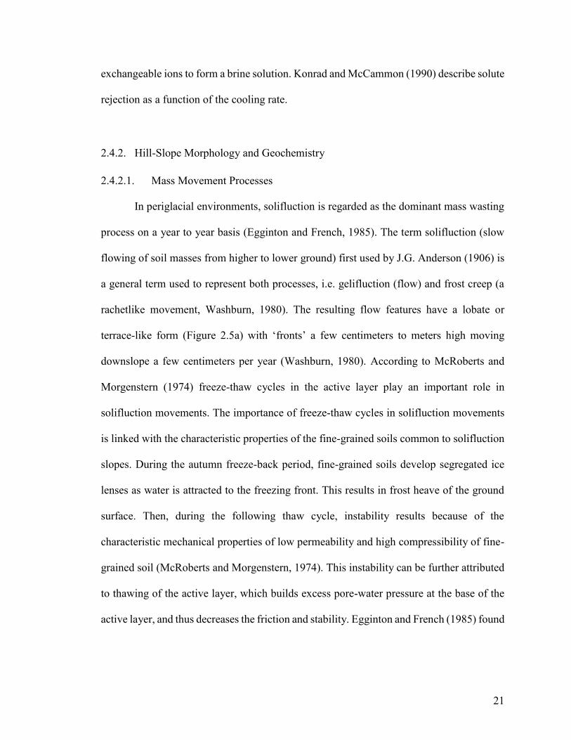
In periglacial environments, solifluction is regarded as the dominant mass wasting
process on a year to year basis (Egginton and French, 1985). The term solifluction (slow
flowing of soil masses from higher to lower ground) first used by J.G. Anderson (1906) is
a general term used to represent both processes, i.e. gelifluction (flow) and frost creep (a
rachetlike movement, Washburn, 1980). The resulting flow features have a lobate or
terrace-like form (Figure 2.5a) with ‘fronts’ a few centimeters to meters high moving
downslope a few centimeters per year (Washburn, 1980). According to McRoberts and
Morgenstern (1974) freeze-thaw cycles in the active layer play an important role in
solifluction movements. The importance of freeze-thaw cycles in solifluction movements
is linked with the characteristic properties of the fine-grained soils common to solifluction
slopes. During the autumn freeze-back period, fine-grained soils develop segregated ice
lenses as water is attracted to the freezing front. This results in frost heave of the ground
surface. Then, during the following thaw cycle, instability results because of the
characteristic mechanical properties of low permeability and high compressibility of fine-
grained soil (McRoberts and Morgenstern, 1974). This instability can be further attributed
to thawing of the active layer, which builds excess pore-water pressure at the base of the
active layer, and thus decreases the friction and stability. Egginton and French (1985) found

22
a)
b)
Figure 2.5 (a) A turf-banked solifluction terrace formed by the slow movement of soil downslope
(near Holman, western Victoria Island, NWT, Canada) (from French, 2007), and (b) mean annual
soil movement (cm/year) for the tops of plastic tubes inserted at Garry Island, N.W.T. for the
(1964–1977) period (from Mackay, 1981).
23
mean surface displacements with an average value of only 0.6 cm/ year over the periods
1972–1983 on the hummocky moraine of eastern Banks Island. Mackay (1981) reported
an average value of up to 1 cm/ year in hummocky centres on Garry Island, N.W.T. (Figure
2.5b). Some rapid and more conspicuous soil movements have also been reported from
Arctic and sub-arctic areas (Williams and Smith, 1991).
2.4.2.2. Hill-Slope Geochemistry
Mass movement processes such as solifluction and the subsurface flow of water
have potential impacts on the geochemical characteristics of hill slopes. Seasonally frozen
ground, (i.e. the active layer) undergoes a series of changes during its winter freezing and
summer thawing. The influence of hill slope morphology on geochemistry could be
explained using two endmember models related to: (a) solifluction, and (b) length of the
flow path.
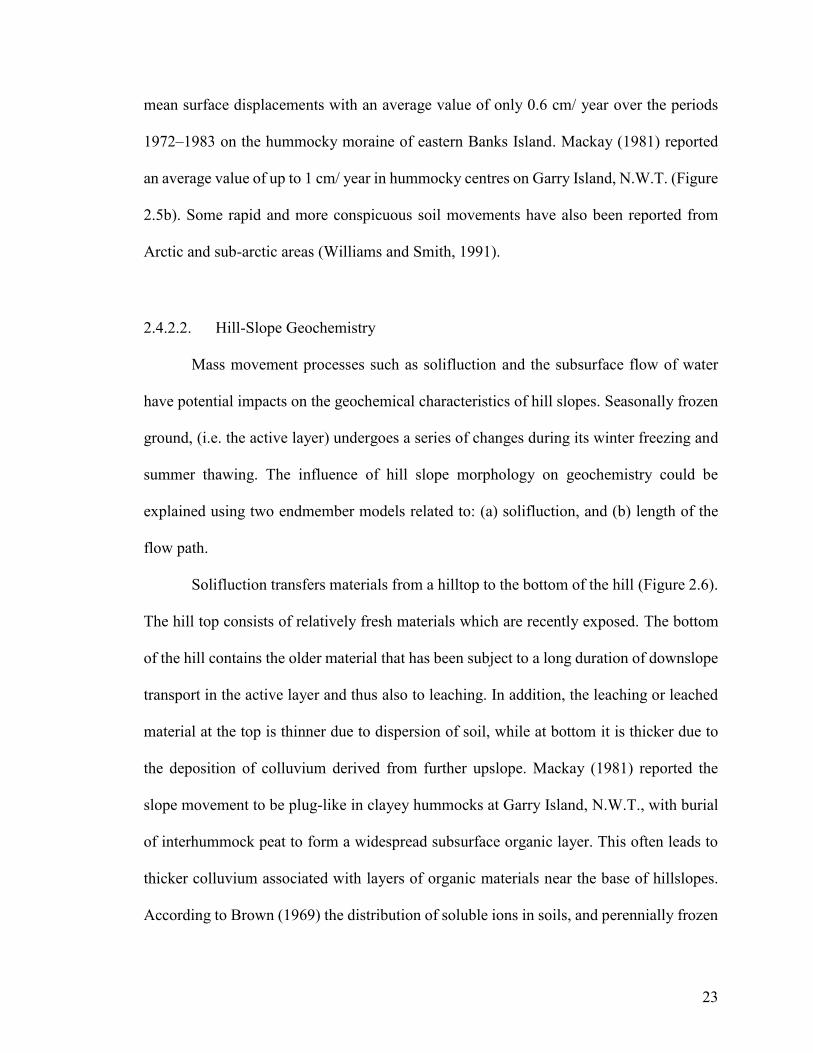
Solifluction transfers materials from a hilltop to the bottom of the hill (Figure 2.6).
The hill top consists of relatively fresh materials which are recently exposed. The bottom
of the hill contains the older material that has been subject to a long duration of downslope
transport in the active layer and thus also to leaching. In addition, the leaching or leached
material at the top is thinner due to dispersion of soil, while at bottom it is thicker due to
the deposition of colluvium derived from further upslope. Mackay (1981) reported the
slope movement to be plug-like in clayey hummocks at Garry Island, N.W.T., with burial
of interhummock peat to form a widespread subsurface organic layer. This often leads to
thicker colluvium associated with layers of organic materials near the base of hillslopes.
According to Brown (1969) the distribution of soluble ions in soils, and perennially frozen

24
ground is influenced by both the material and the present and past depositional and leaching
environments. This suggests that on a hill slope, solifluction may play a significant role in
generating contrasts in geochemical characteristics and soil organic carbon profiles. The
fresh material at the hill top usually has a high soluble ion concentration while the material
at the bottom of the hill is progressively depleted of ions along the pathway.
Second, geochemical contrasts between the points at a hill top and hill bottom also
depend upon the nature and intensity of chemical and biogeochemical weathering, along
the flow path. For example, excessive protons in soil can be produced through various
processes, such as soil respiration (which increases the partial pressure of CO2 in the soil
waters), and pyrite oxidation (which releases H+), which ultimately drives the carbonate
dissolution (Woo and Marsh, 1977; Kling et al., 1992; Huh et al., 1998; and Slutter and
Billet 2003). Similarly, Lacelle et al. (2008) discuss the importance of pCO2 to describe the
difference in ion concentrations between the active layer and near the permafrost table.
This study shows that in the active layer: 1) pCO2 of near-surface groundwater is lower
than that of groundwater near the permafrost table; and 2) pCO2 of the groundwater near
the permafrost table increases as we move downslope, because of the large volume of
meltwaters passing through the sediments. This affects the ion concentrations, being higher
at the bottom of the hill due to higher acidity along a longer flow path, while lower at the
top of a hill due to lower acidity and shorter flow paths (Figure 2.7).
It is expected that both of these processes, i.e. solifluction and water movement,
may occur on hill slopes in periglacial regions on different time scales. In this study,
permafrost samples are collected from diverse locations on hillslopes to determine whether
geochemical conditions vary between erosive and depositional permafrost environments.

25
Figure 2.6 The possible relation between hill slope morphology and geochemistry as explained by
mass movement process (solifluction).
Figure 2.7 The possible relation between hill slope morphology and geochemistry as explained by
water movement along the flow path. The darker longer arrows towards the slope and near the
bottom of the hill represent increasing water content due to increase in the catchment area, and
hence the potential for more leaching due to higher acidity.

26
2.4.3. Organic Matter in the Active Layer and in Permafrost
Cryoturbation is an important process responsible for the transport and
sequestration of organic materials into the active layer and near-surface permafrost
(Bockheim, 2007). The influence of cryoturbation in sequestering organic materials in
permafrost soils normally concerns shallow (1–3 m) depths (Tarnocai et. al., 2009). As the
soil temperature falls below 0 ºC, pore water within the soil successively freezes and
expands. This expansion as well as the formation of ice lenses by water migration to the
freezing front leads to heaving and moves soil towards the surface (upwards). In some
cases, this upward displacement of materials also results to form mound shaped features
known as hummocks (Mackay, 1980). When the ice melts, this results in the subsidence of
the previously frozen soil mass, and materials are transported downwards (Diochon et al.,
2013). This repeated and laterally heterogeneous process of heaving and subsidence
transfers and mixes organic-rich materials from the surface to the bottom of the active
layer, and in some cases to the surface (Diochon et al., 2013). This gives rise to the
characteristically broken or irregular soil horizons commonly associated with
cryoturbation. Large quantities of organic materials can be transported by cryoturbation
into the active layer and from there be incorporated into near-surface permafrost where
conditions are not conducive for decomposition (Kaiser et al., 2007). Other possible
mechanisms include the burial of surface organic matter followed by permafrost
aggradation which transfers organic matter content into the deeper horizons (e.g. Kokelj et
al., 2009; O’Donnell et al., 2011).
There is relatively good understanding of the vertical (soil horizon) partitioning of
the permafrost carbon pool in the upper 3 m of soils. However, deeper carbon pools in

27
unconsolidated Quaternary deposits need to be better constrained (Kuhry et al., 2013). For
example, deltaic, alluvial and yedoma deposits, are predicted to contain large amounts of
organic carbon below 3 m depth (Tarnocai et al., 2009) which are at potential risk of
thawing (Schuur et al., 2008). Several other deposits in permafrost have been reported from
northern Siberia which are predicted to contain large SOC mass (Schirrmeister et al., 2002).
These include the typical ice-rich, fine-grained ‘Yedoma Ice Complex’ of the late
Pleistocene mammoth tundra-steppe, Holocene and Weichselian peat and fluvial deposits,
lacustrine deposits in (former) thermokarst depressions and older Ice Complex deposits.
These deposits vary greatly in carbon contents (0.5–10% of dry weight).

28
CHAPTER 3. STUDY AREA AND METHODS
3.1. Study Area
3.1.1. Location and General Characteristics
The study area is located in the Lac de Gras region of the Slave Geological
Province, Northwest Territories. It is situated north of tree line, approximately 320 km
northeast of Yellowknife and 200 km south of the Arctic Circle. The study area is in the
continuous permafrost zone (Figure 1.1). Permafrost in this region is estimated to be more
than 460 m thick (Canamera Geological, 1996).
The Lac de Gras area lies in the Bear Slave Upland physiographic region of the
Canadian Shield, and is characterized generally by low relief (Hu et al., 2003). The area
was covered by the Laurentide ice sheet and now glacial deposits form the most prevalent
surface materials (Dredge et al., 1999). The region includes a wide range of terrain units
(Figure 3.1). Most of the area is overlain by till often differentiated as till veneer (<2 m
thick), till blanket (2 to 10 m), and hummocky till (5 to 30 m) (Wilkinson et al., 2001).
Similarly, bedrock with a thin, patchy veneer of glacially derived surficial soils is exposed
over a considerable area, and irregular bedrock knobs and cuestas form hills up to 50 m
high (Dredge et al., 1999). Numerous, eskers and outwash complexes are found in the Lac
de Gras area (Dredge et al., 1994). Other terrain types in the region include organic
deposits, peatlands, as well as earth hummocks in valleys. The area also contains some of
the oldest rocks on earth and is well known for a long history related to mining and
development (Karunaratne, 2011). The area is characterized by three main lithological
units, namely: 1) greywacke-mudstone metaturbidites (metasedimentary rocks), 2) biotite-
hornblende tonalite to quartz diorite (diorite), and 3) 2-mica granite and suite (granite to

29
Figure 3.1 Surficial sediments and terrain units in the Lac de Gras area (circle). Modified from
Dredge et al. (1999).

30
granodiorite) (Hu et al., 2003). The metasedimentary rocks in the area belongs to the
Yellowknife Supergroup and are comprised of thinly-bedded metagreywacke to locally
thick-bedded porphyroblastic schists (Kjarsgaard and Wyllie 1994). At the surface,
weathered materials from porphyroblastic schists with a dark grey to green-brown or rusty
brown colour are typically avalable. The granitic rocks are usually light grey, fine to
pegmatitic and are comprised of biotire, muscovite and portions of quartz, plagioclase and
potassium feldspar. Some accessory minerals include apatitite, tourmaline and garnet (Hu
et al., 2003).
3.1.2. Surficial Geology
All glacial features in the Lac de Gras area were conditioned by the Late
Wisconsinan Laurentide ice sheet, which retreated about 9000 years ago (Kerr et al., 1997).
The surficial soils consist predominantly of ablation till or glaciofluvial sediments. The
northern half of the region is dominated by silty sand till deposits while the southern half
consists of granitic bedrock with minor till deposits (Hu et al., 2003). Generally, however,
the till is characterized by a silty sand to sand matrix with low percentages of clay, and
contains 5 to 40% gravel (Wilkinson et al., 2001). Till derived from granitic and gneissic
terrain has a slightly silty, sandy matrix, whereas, till derived from metasedimentary rocks
contains a higher silt-clay content (Dredge et al., 1999).
Solifluction, freeze-thaw cycles and low temperatures have led to a range of
periglacial features such as boulder fields, frost mounds and patterned ground (Hu et al.,
2003). These processes have contributed to the development of large solifluction lobes on
some slopes, especially on the drumlin flanks in terrain underlain by sedimentary rock

31
where the tills are slightly plastic (Dredge et al., 1999). Due to the large modification of
upper 0.5 to 1 m of soil by cryoturbation, organic material has been sequestered at depths
of up to 80 cm (Dredge et al., 1994).
3.1.3. Climate
The regional climate is continental, with summers cool and short, and winters cold
and extremely long (Hu et al., 2003). However, there are differences in the mean annual
air temperature (MAAT), and precipitation across the region. Yellowknife, located
approximately 320 km southwest of Lac de Gras area has a MAAT of -4.2 ºC (1981–2010),
and daily mean temperatures above 0 ºC from May to September (Environment Canada,
2016). July is usually the warmest month (17 ºC), and January is typically coldest (-26 ºC)
(Figure 3.2). Total annual precipitation at Yellowknife is 293 mm and the majority falls in
the summer and autumn (Figure 3.2). In contrast, Lupin, a gold mine in Nunavut
approximately 100 km northwest of Lac de Gras (Figure 3.1), has a MAAT of -10.9 ºC
(1982–2006), and daily mean temperatures above 0 ºC from June to September
(Environment Canada 2016). The warmest and coldest months at Lupin are also July and
January however, with mean monthly air temperatures of 12 ºC and, -30 ºC respectively
(Figure 3.2). Annual precipitation at Lupin is slightly greater than at Yellowknife, with a
total of 298 mm (Figure 3.2). Ekati has a MAAT of -8.9 ºC (1998–2008) with a maximum
monthly temperature of about 14 ºC in July and a minimum monthly temperature of -28 ºC
in January (Figure 3.2) (Environment Canada 2016). Total annual precipitation at Ekati is
275 mm.

32
Figure 3.2 Mean monthly air temperature (circles), and mean monthly precipitation (bars) for
Yellowknife Airport (1981–2010), Lupin Airport (1982–2006) and Ekati Airport (1998–2008)
respectively (Environment Canada 2016).
0
10
20
30
40
50
60
70
Pre
cip
ita
tion (
mm
)
Temperature
Precipitation-4
0-3
0-2
0-1
00
10
20
Yellowknife Climate (1981-2010)
Months
Tem
pera
ture
(ºC
)
Jan Feb Mar Apr May Jun Jul Aug Sep Oct Nov Dec
0
10
20
30
40
50
60
70
Pre
cip
ita
tion
(m
m)
Temperature
Precipitation
-40
-30
-20
-10
01
02
0
Lupin Climate (1982-2006)
Months
Te
mp
era
ture
(ºC
)
Jan Feb Mar Apr May Jun Jul Aug Sep Oct Nov Dec
0
10
20
30
40
50
60
70
Pre
cip
ita
tion (
mm
)
Temperature
Precipitation
-40
-30
-20
-10
010
20
Ekati Climate (1998-2008)
Months
Tem
pera
ture
(ºC
)
Jan Feb Mar Apr May Jun Jul Aug Sep Oct Nov Dec

33
3.1.4. Vegetation
The project area is characterized mainly by continuous shrub tundra (Wiken et al.,
1996). Common shrubs in the area include Northern Labrador Tea (Rhododendron
tomentosum), and Dwarf Birch (Betula glandulosa), while Bog Cranberry (Vaccinium
vitis-idaea) and Dwarf Bog Rosemary (Andromeda polifolia) are the dominant short shrubs
(Karunaratne, 2011). The upland areas are often covered with a thin layer of lichens and
mosses, due to well-drained soil conditions (Hu et al., 2003). Sphagnum spp. mosses also
colonize many wetlands (Karunaratne, 2011). The most common species of lichens are
Cladina spp. and Cladonia spp. while Aulacomnium turgidum and Rhacomitrium
lanuginosum are the typical mosses (Karunaratne, 2011). Vegetation in valleys and
low-lying areas consists mainly of coarse grasses, mosses, and peat, due to poorly-drained
soil conditions (Hu et al., 2003). The vegetation is lush along drainage courses, and in wet
areas where willows (Salix spp) can be as tall as 2 m (Hu et al., 2003). In addition, low-
lying depressions in this area also have thick deposits of peat associated with ice-wedge
polygons and sedge meadows, underlain by fine-grained materials (Karunaratne, 2011).
3.1.5. Permafrost
In the Lac de Gras area, permafrost is estimated to be more than 460 m thick
(Canamera Geological, 1996), however this varies considerably depending on local site
conditions. Factors such as the mean annual ground temperature, thermal properties of
earth materials, and proximity to water bodies contribute to this variability (Williams and
Smith, 1991). The mean annual ground temperatures at a depth of 20 m range between -3
ºC to -6 ºC (Hu et al., 2003). The depth of the active layer varies with vegetation cover,
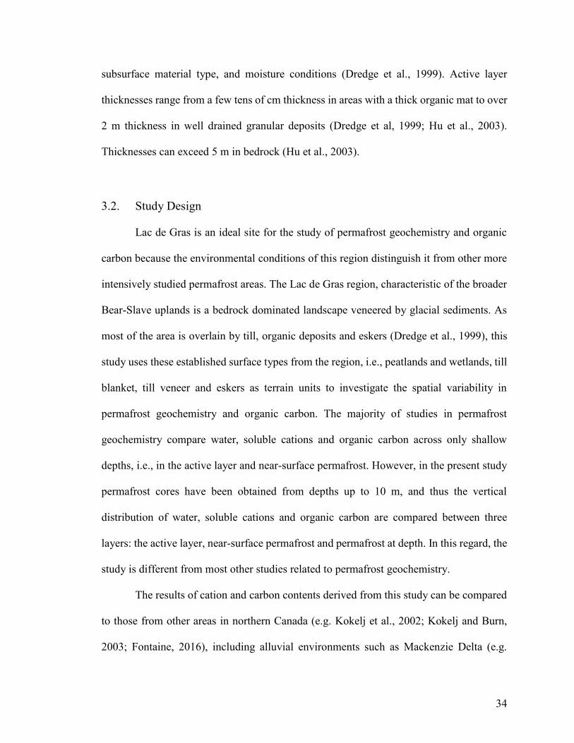
34
subsurface material type, and moisture conditions (Dredge et al., 1999). Active layer
thicknesses range from a few tens of cm thickness in areas with a thick organic mat to over
2 m thickness in well drained granular deposits (Dredge et al, 1999; Hu et al., 2003).
Thicknesses can exceed 5 m in bedrock (Hu et al., 2003).
3.2. Study Design
Lac de Gras is an ideal site for the study of permafrost geochemistry and organic
carbon because the environmental conditions of this region distinguish it from other more
intensively studied permafrost areas. The Lac de Gras region, characteristic of the broader
Bear-Slave uplands is a bedrock dominated landscape veneered by glacial sediments. As
most of the area is overlain by till, organic deposits and eskers (Dredge et al., 1999), this
study uses these established surface types from the region, i.e., peatlands and wetlands, till
blanket, till veneer and eskers as terrain units to investigate the spatial variability in
permafrost geochemistry and organic carbon. The majority of studies in permafrost
geochemistry compare water, soluble cations and organic carbon across only shallow
depths, i.e., in the active layer and near-surface permafrost. However, in the present study
permafrost cores have been obtained from depths up to 10 m, and thus the vertical
distribution of water, soluble cations and organic carbon are compared between three
layers: the active layer, near-surface permafrost and permafrost at depth. In this regard, the
study is different from most other studies related to permafrost geochemistry.
The results of cation and carbon contents derived from this study can be compared
to those from other areas in northern Canada (e.g. Kokelj et al., 2002; Kokelj and Burn,
2003; Fontaine, 2016), including alluvial environments such as Mackenzie Delta (e.g.

35
Smith, 1975; Kokelj and Burn, 2005), or regions with thick carbonate-derived tills (Kokelj
and Burn, 2003; Lacelle et al., 2013). Therefore, patterns of geochemistry and organic
carbon from the Lac de Gras region can be compared with these contrasting depositional
environments.
3.2.1. Site Selection
The selection of sites was based on the LiDAR and imagery dataset provided by
the Dominion Diamond Ekati Corporation. LiDAR data was collected in twelve flights
between July 23rd and August 11th 2013, and was made available at 1 m grid resolution. As
the surficial conditions (relief, vegetation, drainage, snow, soil and rock characteristics)
play a significant role in determining the conditions of permafrost, the collected data were
interpreted in the context of the following attributes: slope-angle, potential direct solar-
radiation, and Topographic Wetness Index (TWI) computed from the LiDAR data. In
addition, a Landsat-derived index outlining the location of late-lying snow drifts was
available for the area. This helped in determining landscape variability and prioritizing
areas representative of different environmental settings including a range of moisture,
vegetation and soil conditions in peatlands, hilltops, hill slopes, hill bottoms, highly
vegetated surfaces, and earth hummocks and depressions, which were then used for site
selection and borehole placement. Twenty-four boreholes were selected using this
approach in different terrain types such as peatlands and wetlands, till blankets, till veneer
and eskers. The location of boreholes across various terrain types is shown in Figure 3.3.

36
3.2.2. Limitations of Site Selection
There are several limitations associated with the site selection of this study. For
example, no boreholes were drilled in block fields despite their importance in the
landscape. Furthermore, problems arose when attempting to drill at many sites from Hill 2
and Hill 3 groups. At Hill 2 and Hill 3, there were some boreholes which got obstructed
when drilled to a few centimeters because they were underlain by bedrock. As a result, they
had to be abandoned. This affected the total number of boreholes available and the diversity
of surface conditions that are sampled.
3.2.3. Site Grouping Details
Boreholes were grouped according to their proximity to each other and respective
terrain types to provide an idea of the geographical location of boreholes. This was also
carried out to facilitate the comparison of water content, soluble cations and organic carbon
across sites within the same terrain type. For example, two different sites from till blanket
terrain could be compared with each other between a hilltop and hill bottom. Table 3.1
shows seven site groups used for the current study. The Control group represents two
boreholes that were drilled next to each other (within 5 m distance) in peatlands and
wetlands. Peatland is a term used to encompass peat-covered terrain (Rydin et al., 2013).
A wetland is defined as: land that is saturated with water long enough to promote wetland
or aquatic processes as indicated by poorly drained soils, hydrophytic vegetation and
various kinds of biological activity which are adapted to a wet environment (National
Wetlands Working Group 1988). Hill 1 represents six boreholes drilled at various locations
within a till blanket in hilly terrain near the Control group. Hill 3 represents two boreholes

37
Figure 3.3 Locations of boreholes used for this study in the Lac de Gras area. The grey hillshade
shows the area covered by the LiDAR DEM. The diamond mine (Ekati) infrastructure as well as
areas not covered in the DEM acquisition are shown by white spaces.

38
Table 3.1 Site groups representing boreholes located within proximity and similar
regional setting
Site Groups Borehole ID (NGO-DD15- )
Control 1006, 1007
Hill 1 1004, 1005, 2004, 2005, 2006, 2007
Hill 2 1014, 2018
Hill 3 2009, 2033
Valley 1009, 1010, 2011, 2012, 2013, 2015,
2016, 2019
Esker 1 2008, 2028, 2029
Esker 2 2026

39
in a till blanket in hilly terrain to the east of the control group. Boreholes drilled at both hill
sites reflected a range of surface conditions with respect to their slope, solar radiation,
steepness, vegetation and wetness index. In addition, both Hill 1 and Hill 3 sites
were characterized by frost boils and small solifluction lobes. Figure 3.4 shows the
boreholes in the Control group, Hill 1 and Hill 3. Hill 2 represents two boreholes in a till
veneer. The Valley group contains the largest number of boreholes drilled in two transects
having varying slope, radiation, snow drift persistence and wetness conditions. Figure 3.5
shows the location of Hill 2 and the Valley. Finally, Esker 1 and Esker 2 represent four
boreholes that are drilled in two different esker complexes. Figure 3.6 and Figure 3.7 show
the location of the two esker sites.
3.2.4. Site Classification
Four different terrain types were compared, i.e., peatlands and wetlands, till
blanket, till veneer and eskers. Previous studies related to geochemistry employed various
formats to compare the sites of interest. For example, at Herschel Island sites were
classified as disturbed vs. undisturbed terrain based on the range of surface conditions
encountered on the island (Kokelj et al., 2002). In the Mackenzie Delta region, a range of
forest-terrain types were considered as terrain types for site classification (Kokelj and Burn,
2005). In the present study, sites were classified on the basis of established terrain units
that were local to Lac de Gras area (Figure 3.1, Table 3.2). This was done in order to
represent a heterogeneous landscape, through sampling of different terrain types, to
investigate the spatial variability that exists in water, organic carbon and soluble cations.

40
Figure 3.4 Borehole locations from the Control group, Hill 1 and Hill 3.
Figure 3.5 Borehole locations Hill 2 and Valley. The Valley group contains the largest number of
boreholes drilled in two transects across various regional conditions.

41
Figure 3.6 Esker 1, where 3 boreholes were drilled in proximity to compare the small-scale
variability in geochemistry and organic carbon.
Figure 3.7 Location of Esker 2 containing a single borehole in its terrain.

42
Table 3.2 Site classification of boreholes based on the terrain units
Terrain Units Borehole ID (NGO-
DD15- )
Includes Site
Groups From
Total Number of
Boreholes
Till Blanket 1004, 2004, 2005, 2006,
2007, 2009, 2033
Hill 1 and Hill 3 7
Till Veneer 1014, 2013, 2016, 2018,
2019
Hill 2 and Valley 5
Peatlands and
wetlands
1005, 1006, 1007, 1009,
1010, 2011, 2012, 2015
Control group, Hill
1 and Valley
8
Eskers 2008, 2028, 2029, 2026 Esker 1 and Esker 2 4

43
3.3. Field Methods
3.3.1. Plot Design
Upon arrival at the field site a 15 m by 15 m plot was centered around the borehole
location and was delineated by wooden dowels placed in each corner. For each plot,
observations of vegetation, topography, and surficial permafrost features were recorded. In
addition, photographs were taken from all four sides of the plot facing towards the North,
South, East, and West for reference. Following this, two soil pits were dug just outside the
plot, aiming to sample similar surface conditions to those of the plot. A graphical
representation of the plot design is shown in Figure 3.8. The idea behind selecting two
extra soil pits was to carry out additional active layer measurements which would have
been difficult to carry out at the drill site. A brief explanation of the measured variables
from the exterior pit is given in Section 3.3.4.
3.3.2. Borehole Core Extraction
Borehole drilling was carried out using a diamond drilling rig (Kryotek Compact
Diamond Sampler) operated by field drillers and an Aurora Geosciences geologist (Figure
3.9). This drilling machine extracts cores of 5 cm diameter. The length of the core segment
was measured for every run using a measuring tape after it was removed from the barrel
(Figure 3.9). Similarly, the depth of the borehole was measured after each run by sliding
the measuring tape to the bottom of the borehole and taking the reading. When drilling to
greater depths, the depth of the borehole was determined by first measuring the core
segment of the barrel placed at the bottom of a run and adding the length of the barrel
stacked on top.

44
a)
b)
Figure 3.8 (a) Graphical representation of the plot design; (b) the position of the exterior pit
varies at each site depending upon the surface conditions.
N

45
a)
b)
Figure 3.9 (a) Field use of diamond drilling rig (Kryotek Compact Diamond Sampler); (b) typical
core segment.

46
All core segments were sectioned into 20 cm intervals using a hammer and a chisel.
The sectioned cores were examined carefully to record their general characteristics. This
included soil type (texture), colour, ice content and visible organic matter. All records were
maintained in a well-labelled drill log sheet. An example of a log sheet is attached in the
Appendix A. After this, each section was kept in a well-labelled sample bag, which was
doubled to avoid any leakage. Finally, the sample bags were made ready for transport to a
laboratory in Yellowknife.
3.3.3. Limitations of Field Measurements
There are some uncertainties associated with field measurements in this study.
Discrepancies existed between the total length of the core segments and the borehole depth.
This was especially the case in lower parts of the boreholes. As core segments would stick
to the bottom of the borehole, they had to be broken up into pieces to take them out. As
a result, core segments would break, introducing a measurement error. Similarly, ice rich
samples would often stick into the barrel so they had to be hammered many times before
they could be taken out. Core segments were sometimes broken and accurate measurements
could not be made. When there were discrepancies between the measurements, the
borehole depth was used to determine the length of the core segment. Lastly, the depth of
thaw at the time of sampling could not be measured accurately at the drilled locations.
However, the sectioned cores were classified as being either frozen or unfrozen and the
respective samples from permafrost and the overlying layers were distinguished.
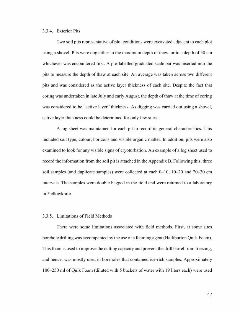
47
3.3.4. Exterior Pits
Two soil pits representative of plot conditions were excavated adjacent to each plot
using a shovel. Pits were dug either to the maximum depth of thaw, or to a depth of 50 cm
whichever was encountered first. A pre-labelled graduated scale bar was inserted into the
pits to measure the depth of thaw at each site. An average was taken across two different
pits and was considered as the active layer thickness of each site. Despite the fact that
coring was undertaken in late July and early August, the depth of thaw at the time of coring
was considered to be “active layer” thickness. As digging was carried out using a shovel,
active layer thickness could be determined for only few sites.
A log sheet was maintained for each pit to record its general characteristics. This
included soil type, colour, horizons and visible organic matter. In addition, pits were also
examined to look for any visible signs of cryoturbation. An example of a log sheet used to
record the information from the soil pit is attached in the Appendix B. Following this, three
soil samples (and duplicate samples) were collected at each 0–10, 10–20 and 20–30 cm
intervals. The samples were double bagged in the field and were returned to a laboratory
in Yellowknife.
3.3.5. Limitations of Field Methods
There were some limitations associated with field methods. First, at some sites
borehole drilling was accompanied by the use of a foaming agent (Halliburton Quik-Foam).
This foam is used to improve the cutting capacity and prevent the drill barrel from freezing,
and hence, was mostly used in boreholes that contained ice-rich samples. Approximately
100–250 ml of Quik Foam (diluted with 5 buckets of water with 19 liters each) were used

48
for a 5 m borehole. Quik Foam is a proprietary blend of alcohol ethoxy sulphates (AES
CnH2n(C2H4O)mSO4X), where n=12–18, m= 0–8 and X = sodium, ammonium or
triethanolamine. As the foam used in the current drilling belonged to a sodium salt grade,
some boreholes were contaminated with some amount of sodium.
In order to determine the level of contamination on the samples, an analysis was
conducted on Quik Foam, with concentrations of soluble cations measured at different
dilution limits (Table 3.3). The contamination was evident at different dilution limits
especially for K+ and Na+ ions. The concentration of Ca2+ and Mg2+ was negligible to
almost < 0.1 mg/ l at all three dilution limits. During field drilling, an average of 175 ml of
foam was diluted with 95 l of water for each borehole. This implies about 542 ml of water,
per ml of foam, which is more than 500 times diluted. With the expected concentration at
500 times dilution, the contamination on the actual samples were predicted to be low due
to the higher dilution (Table 3.3).
A separate lab experiment was carried out at Carleton University’s Geocryology
Laboratory in order to determine the amount of foam attached to a given volume of the
frozen core segment after it is dipped in a foam mixture. This was done by weighing the
frozen core, dipping it into a foam mixture and finally weighing it again to compare the
weight gained. Table 3.4 reports the mass of frozen cores before and after dipping into the
foam mixture. The experiment was performed two times with five and four replicates,
respectively. A decrease in the mass of sample was observed at both trials after the samples
were dipped into the foam mixture. This experiment shows that at least some of the foam
which is attached to the outer surfaces of the frozen core flows away along with ice
melt and causes a decrease in the total mass. Because the duration in the field is much

49
longer from the time core segments are taken out from the barrel to examining their general
characteristics and finally bagging, most of the foam attached to the outer surfaces of the
cores likely runs off during the sample handling time.
The two different analyses on the foam showed that the concentration of K+ and
Na+ in the actual sample should be relatively low due to higher dilution (nearly 500x), and
running off of the foam during sample handling time.
Additional limitations of the field methods included irregular sampling intervals
(core sectioning) for core segments of few boreholes. Occasionally, core segments would
contain either bedrock, or boulders extending few cm in between soil samples and
therefore, had to be discarded. Whenever, if this was the case, a note was made on a
particular section. This included recording the material type and its length.
Finally, active layer depths could not be measured directly from the boreholes. This
is because core barrels were longer than a meter length with only 5.5 cm diameter, making
accurate measurements of the active layer impossible in the borehole itself. However,
qualitative estimates of active layer depths were made when core segments were taken out
from the barrel. This was done by examining the core segment and classifying it as being
either frozen or unfrozen. The length of the unfrozen core segment obtained from the first
run was considered as the thickness of the active layer. Lastly, the excess ice content
reported in this study is a minimum estimate because at many instances, some ice was lost
due to the drilling heat. This was mainly the case when drilling at sites from till blanket
and till veneer terrains.

50
Table 3.3 Measuring the concentration of major ions (mg/ l) at different dilution limits
Soluble Ions 50x 75x 100x Expected at 500x
Calcium < 0.1 < 0.1 < 0.1 < 0.1
Magnesium < 0.1 < 0.1 < 0.1 < 0.1
Potassium 143 135 125 14.3–25.0
Sodium 107 101 90.6 10.7–18.1
Table 3.4 Trial experiment reporting the mass of frozen cores before and after dipping in
a foam mixture
First Trial
Initial Mass (g) Final Mass (g)
729.91 728.84
703.71 702.81
690.35 689.38
682.58 681.73
675.88 674.74
Second Trial
Initial Mass (g) Final Mass (g)
900.55 900.44
874.96 874.89
825.64 825.60
801.63 800.93

51
3.4. Laboratory and Analytical Methods
3.4.1. Soil Water Sampling
A few samples collected from the field were first used in an experiment to compare
three distinct soil water extraction techniques for geochemical analysis. Method 1 and
Method 2 are commonly used methods in soil science for the extraction of soil water.
Another method (Method 3) was also tested to compare cation concentrations obtained
from all three methods. The experiment was performed using eight permafrost samples
with sample numbers (162-5, 162-6, 163-3, 163-4, 164-9, 164-11, 165-4, and 165-17) at
Carleton University’s Geocryology Laboratory.
In Method 1, permafrost samples were thawed and homogenized, poured into
beakers, weighed, and allowed to settle for 12 h. Supernatant water was extracted from
thawed permafrost samples using a syringe and filtered through 0.45 μm cellulose filter
paper. Supernatant water was extracted from four samples (163-3, 164-9, 164-11, and 165-
4), which were vialed separately for analysis. One of the drawbacks of this method is that
not all samples contain supernatant water and, therefore, some samples need to be
processed with other methods such as Method 2 or Method 3 for soil-water extraction. In
order to facilitate the comparison of solute concentrations obtained from the three water
extraction techniques, gravimetric water content “at extraction” and the “field” moisture
content were determined for samples that required deionized water.
In Method 2, all samples were oven dried and a known amount of deionized water
was added to make a saturated paste (~1:1 extraction ratio by mass; Janzen 1993). All
samples were mixed thoroughly, and the samples were reweighed. The sediment was
allowed to settle for 12 h, and excess water was then collected with a syringe and filtered

52
through 0.45 μm cellulose filter paper for geochemical analysis. A drawback associated
with this method is the likely possibility of reduced dissolution of ions into the soil-water
after drying.
In Method 3, samples were subject to a direct addition of a known amount of
deionized water (~1:1 extraction ratio by mass; Janzen 1993). All samples were mixed
thoroughly, and the samples were reweighed. The samples were allowed to settle for 12 h,
and excess water was extracted with the help of a syringe and finally, filtered through 0.45
μm cellulose filter paper. Four samples (162-5, 162-6, 163-4, and 165-17) underwent this
method for the extraction of water which were kept in different vials. The extracted water
from all three methods were sent to a lab for the analysis of soluble cations. A drawback
associated with this method is a likely possibility of causing additional ion uptake due to
reduced concentration after dilution.
The results obtained from this experiment indicate that concentrations of soluble
cations obtained from Method 1 and Method 2 are relatively similar and distinct from
Method 3 (Figure 3.10). Method 2 has the advantage of providing standardization for better
comparability, but the disadvantage of possibly subduing high ion content present in soil-
water. Method 1 is a desirable method, however, not practical as some samples do not
contain supernatant water. Toner et al. (2013) describe that in the water extraction with
Method 3 the resulting concentration of soluble ions changes with the extraction ratio
chosen as samples are usually not fully leached out. Because this thesis aims to determine
the pore water characteristics in active layer and permafrost samples (to infer the amount
of solutes released into the environment, if the permafrost were to thaw), and not the
potential to release ions during leaching over time, Methods 1 and 3 were considered

53
Figure 3.10 (a) Calcium concentration; (b) magnesium concentration; (c) potassium concentration; and (d) sodium
concentration measured with three methods. (e) relative difference of Method 2 with Methods 1 and 3. Square
represents 2 with 1, while triangles represent 2 with 3. Orange, green, blue and red denotes sodium, calcium,
potassium and magnesium ions respectively. Concentrations obtained from Method 2 and Method 3 were corrected
to original “field” water contents.
162-5 162-6 163-3 163-4 164-11 164-9 165-17 165-4
020
40
60
80
10
0120
140
Ca2+
concentration
Sample ID
Concen
tra
tion (
mg/l)
Method 1
Method 2
Method 3
a)
162-5 162-6 163-3 163-4 164-11 164-9 165-17 165-4
01
02
030
40
50
60
Mg2+
concentration
Sample ID
Method 1
Method 2
Method 3
b)
162-5 162-6 163-3 163-4 164-11 164-9 165-17 165-4
02
00
40
06
00
80
01
000
K+ concentration
Sample ID
Co
nce
ntr
atio
n (
mg/l)
Method 1
Method 2
Method 3
c)
162-5 162-6 163-3 163-4 164-11 164-9 165-17 165-4
010
020
03
00
400
50
060
0
Na+ concentration
Sample ID
Method 1
Method 2
Method 3
d)
162-5 162-6 163-3 163-4 164-11 164-9 165-17 165-4
-2-1
01
2
Relative difference of Method 2 with Methods 1 and 3
Sample ID
Re
lative
diffe
ren
ce
e)
54
appropriate for obtaining water for the determination of the concentration of soluble cations
in cases with strongly differing soil-water contents.
3.4.2. Core Samples (Boreholes + Exterior Pits)
In the laboratory (EBA, Yellowknife), thawed permafrost samples were
homogenized, poured into beakers, weighed, and allowed to settle for 12 h (e.g. Kokelj and
Burn, 2003). A qualitative estimate of sediment texture and organic matter was also made
and recorded. Following this, samples were processed to estimate the excess-ice content.
3.4.2.1. Excess-Ice Content
The excess-ice content was determined for each ice-rich sample from the boreholes.
Volumes of sediment and supernatant water were recorded to estimate excess ice content
Ic (%) as follows (e.g. Kokelj and Burn, 2003):
(2) 𝐼𝑐 (%) = (𝑊𝑣 ∗ 1.09) / (𝑆𝑣 + (𝑊𝑣 ∗ 1.09)) ∗ 100
where Ic (%) is the excess-ice content expressed on a volumetric basis, Wv is the volume
of supernatant water, Sv is the volume of saturated sediment and 1.09 represents the density
of water divided by that of ice.
3.4.2.2. Soil Water Extraction
After the comparison of results obtained from the Soil Water Sampling, Method 1
and Method 3 were considered as appropriate methods to obtain soil water for geochemical
analysis. This section provides further details on the methods used to extract soil water
from all core samples. Method 1 was used to extract supernatant water from thawed
permafrost samples. A known amount of deionized water was added to active layer and

55
permafrost samples that were not supersaturated (~1:1 extraction ratio; Janzen 1993,
Method 3). All samples were mixed thoroughly, and were allowed to settle for 12 h. The
excess water was then collected with a syringe and filtered through 0.45 μm cellulose filter
paper for geochemical analysis. Since, the “original” field moisture content and the water
content “at extraction” were determined for each core sample, the concentration of soluble
cations obtained from Method 3 were corrected to “field” water contents using the steps
below:
Step 1 – Original water content in the sample
(3) 𝑂𝑟𝑖𝑔𝑖𝑛𝑎𝑙 𝑤𝑎𝑡𝑒𝑟 = {(𝐺𝑊𝐵 (%) ∗ 𝑚𝑤𝑠) / 100}
where original water is the mass of water (g) at field conditions, GWB (%) is the percentage
gravimetric water content expressed on a wet-basis and mws is the mass of field-moist soil
(g).
Step 2 – Total water mass
(4) Total water = Original water + Added water
Where total water is the mass of total water (g) contained in a sample and added water is
the mass of water (g) that were added to samples which were not supersaturated.
Step 3 – Correction factor
(5) Correction factor = Total water / Original water
where correction factor is the correction for the original water in a sample depending upon
total water contained.

56
3.4.2.3. Electrical Conductivity
The electrical conductivity (mS/cm) was measured on all water extracts after
filtering with a Yellow Springs Instruments Model 30 conductivity-salinity probe,
calibrated daily against an NaCl reference solution. Since conductivity is proportional to
the amount of electrolyte in solution, its measurement can be indicative of total soluble
cations (sum of soluble Ca2+, Mg2+, K+ and Na+) in soil-water extractions (Janzen, 1993).
The values of conductivity (mS/cm) were corrected to the original water content in the
samples:
(6) Field conductivity (mS/cm) = measured Conductivity * Correction factor
where correction factor is the correction for the original water in a sample depending upon
total water contained.
3.4.2.4. Gravimetric Water Content
Gravimetric water content-dry basis (GWCD) was determined for each core sample
using the oven drying method. Each sample was weighed in the lab, oven dried at 105º C
for 24 h and reweighed to determine the GWCD. The GWCD was obtained by dividing the
mass of water (mw) given by difference between wet and dry masses by the mass of the dry
soil.
(7) GWCD = mw/mds
where GWCD is the gravimetric water content expressed on a dry-basis, mw is the mass of
water (g), mds is the mass of oven-dried soil (g).
In ice-rich soil, GWCD can produce values that greatly exceed 100%, which are
difficult to interpret (Phillips et al., 2015). Therefore, gravimetric water content was also

57
expressed on a wet-basis, i.e., Gravimetric water content-wet basis (GWB). The water
content GWB was obtained by dividing the mass of water by wet or field weight of the
sample.
(8) GWB = mw/mws
where GWB is the gravimetric water content expressed on a wet-basis, mw is the mass of
water (g), mws is the mass of field-moist soil (g).
3.4.2.5. Soluble Cation Concentrations
The concentration of soluble cations (i.e. Ca2+, Mg2+, Na+ and K+) was determined
on all soil water extracts using an atomic adsorption spectrophotometer at the Taiga lab in
Yellowknife. Since, the moisture content at extraction was determined for each core
sample, the concentration of soluble cations obtained from Method 3 were corrected to
original “field” water contents using the steps below:
Step 4 – Concentration of soluble cations with respect to “field” water contents
(9) CCFWC = Reported concentration * Correction factor
where CCFWC is the concentration of soluble cations in (mg/l) after correction to field
water concentration. Reported concentration is the concentration of soluble cations in
(mg/l) before correction and correction factor is the correction for the original water in a
sample depending upon total water contained.
Soluble ion concentrations in soil-water extractions were also converted to milli-
equivalents per unit weight of dry soil (meq/ 100g of dry soil). First, the reported
concentration of soluble cations in (mg/l) were converted to (meq/l) by the equation:
(10) 𝐶𝐶𝐸𝑄𝐿 = 𝐶𝐶𝐹𝑊𝐶𝐸𝑞𝑊𝑡.⁄

58
where CCEQL is the concentration of soluble cations in milli-equivalents per liter of water,
CCFWC is the concentration of soluble cations in milli-grams per liter of water and EqWt.
is the equivalent weight of ions in grams.
Finally, the results of ions from CCEQL were converted to C(meq/100 g of dry
soil) by the equation:
(11) 𝐶𝐶𝐸𝑄𝐷𝑆 = 𝑊𝑚 ∗ 𝐶𝐶𝐸𝑄𝐿
where CCEQDS is the concentration of soluble cations expressed in milli-equivalents per
unit weight of dry soil (meq/ 100g of dry soil), Wm is the mass of water per 100 g of dry
soil and CCEQL is the concentration of soluble cations in milli-equivalents per liter of
water. Presentation of soluble cation concentrations per unit weight of dry soil (meq/ 100g)
facilitated comparison of solute concentration between core samples of varying moisture
contents.
3.4.2.6. Organic Matter Content
Organic matter content was determined for all core samples using the sequential
loss-on ignition method (Sheldrick, 1984) at Carleton University. A small amount (2–3) g
of the oven dried sample (< 0.5 mm soil fraction) was placed in a crucible and heated to
550 ºC in a high-temperature muffle-furnace for 6 h (Figure 3.11). However, some samples
from the exterior pits were highly organic in nature and hence, in these cases crucibles
were filled to only 1/4. The crucible was allowed to cool in a desiccator and was then
reweighed, and the organic matter content was determined according to (Sheldrick, 1984):
(12) LOI = ((SOD – Si) / SOD) * 100

59
a)
b)
Figure 3.11 (a) Sample being weighed in a crucible; (b) crucibles inside a muffle furnace ready to
undergo LOI 550.

60
where LOI is the % Loss-on-ignition, SOD is the mass of sediment after oven drying at 105º
C, and Si is the sediment mass after ignition at 550 ºC.
3.4.3. Soil Textural Analysis
Soil type is an important control on hydraulic conductivity as it governs pore size
distribution and water content below 0º C, and therefore the potential for ice segregation
and ground water movement. Finer-textured soils with moderate permeability and porosity
(e.g. frost susceptible silts) allow unfrozen water to move towards a freezing front, and
this process is responsible for the formation of segregation ice. In this study, selected
samples from boreholes were analyzed for soil texture to examine whether water and
excess ice contents at sites from various terrains were related to their soil textures. This
provided the context for the present research, to examine the spatial variability of water
content (including excess ice) between different terrain types based on their soil properties.
The soil texture was analyzed using the laser diffraction (LD) method (e.g. Eshel et al.,
2004).
Soil subsamples were taken from each borehole based on the total depth of the
borehole, and spatial continuity of the sample distribution (sample types). To do this,
samples were first identified from different depth intervals i.e. near-surface (< 2 m),
shallow (2–4 m), and deeper permafrost (> 4 m) depending upon the total depth of the
borehole. Second, the spatial continuity of sample distribution was examined within each
interval by looking at the drill logs that were prepared during the field measurements. A
total of 59 samples were selected from 24 boreholes for the analysis of grain size which
represented a range of soil types, and depth intervals found within each borehole.

61
Each sample was first oven dried at 105º C, and then crushed and homogenized in a
mortar. The sample was then passed through a 2 mm sieve to remove any coarse particles.
This was followed by the removal of organic matter using hydrogen peroxide. The samples
were then mixed with calgon to prevent flocculation and passed through a Beckman
Coulter LS 13 320 Laser Diffraction-Particle Size Analyzer for the grain size analysis.
3.5. Data
3.5.1. Quality Control
Field sampling, analysis of samples, and processing of the data, followed
established protocols. In the field, written protocols were used to maintain proper sampling
and for recording of the information and sample bagging. Core samples were
photographed, double-bagged and labelled properly to avoid any leakage or loss. Similarly,
samples from each borehole were kept in a well-labelled pail until delivered to the
laboratory.
Specific protocols were developed and handed to the EBA lab to assist sample
preparation and analysis. This included step-wise instructions to prepare samples for the
lab analysis of cations and soil organic matter. Gravimetric and volumetric measurements
were used to derive the gravimetric water content and excess ice content in the samples.
The protocol is presented in Appendix C. Test methods and data used by the Taiga lab are
regularly validated by the Laboratory Quality Assurance Program. All the routine methods
are based on recognized procedures from sources such as Standard Methods for the
Examination of Water and Wastewater APHA (American Public Health Association),
AWWA (American Water Works Association), WEF (Water Environment Federation),

62
Environment Canada and USEPA (US Environmental Protection Agency). A regular
correspondence was maintained with labs with the updated results and comments to ensure
proper lab analysis at all times.
During the processing of the data, the original results (.xlsx files) from the Taiga
lab were kept in a separate folder and renamed as “original results” to ensure no changes
were made. Secondary files were created and renamed as “import sources” so that they
could to be modified and read for data analysis using the software package R. The changes
were recorded in a separate file known as the “modification catalog”.
3.5.2. Presentation of the Data
Data for this study is presented by site groups as described in Section 3.2.2, and is
placed in the Appendix D. The first part of the data is the field data which is presented in
tables. The field data includes site number, geographic location and elevation (from survey-
grade GPS + PPP), terrain conditions, surface topography and vegetation conditions at each
site. Next, field and laboratory data from each borehole are presented in plots. Each plot
contains the information on the active layer depth (indicated by a dashed line), Unitcode (a
visual description of permafrost samples as recorded by the field geologists in their drill
logs), total soluble cations (meq/100 g of dry soil), soil-water conductivity (mS/cm,
standardized to the original water content in the samples), gravimetric water content (%,
expressed on a gravimetric wet basis) and excess ice content (%, gravimetric basis), and
organic matter content (%, expressed on a dry basis). The Unitcode provides an idea of the
type of sample recovered, a rough estimate of soil texture, excess ice content and their
types, and any organic materials recorded. Similarly, small symbols vs. larger symbols

63
have been used in the plots to represent the samples from the exterior pits vs. boreholes.
Gravimetric water content and excess ice content are plotted on the same graph for ease of
understanding water and ice content in a sample. Only the recovered samples are plotted,
and unrecovered drill intervals are left blank.

64
CHAPTER 4. RESULTS
4.1. Overview
The results are organized into four sections. Following this introduction, the second
section presents the results of the grain size analysis that was conducted on selected
samples. The results of this analysis provide an idea of soil textures of samples from each
site, and guides comparison of spatial variability in water and excess ice, organic matter
and soluble cation content between terrain types. The third section reports the values of
measured variables at sites to describe their vertical distribution, including the contrast
between the active layer, near-surface permafrost and the permafrost at depth. Further, the
section also incorporates the results of the statistical analyses conducted in order to
compare the spatial variability of observed water, organic matter and ion contents between
terrain types. Finally, the last section describes the observed correlations between the water
content GWB, organic matter content and cation contents.
4.2. Grain Size and Soil Texture
The results of the grain size analyses are presented in Appendix E, classified
according to the USDA textural classification system (2 mm > sand > 53 μm > silt > 2 μm
> clay). The results indicate that on average, soils consist of poorly to very poorly sorted
silt and sand. The mean grain size of samples from four different terrains was quite variable
with highest of 212 µm from eskers and the lowest of 83 µm from peatlands and wetlands
(Appendix E). The relative proportion of silt was quite high among peatlands and wetlands,
and till veneer terrains. Clay percentage was < 18% among all four terrain types.
A textural ternary plot is presented in Figure 4.1. On average, the soil texture was
classified to be “sandy loam” for peatlands and wetlands and till veneer, and “loamy sand”
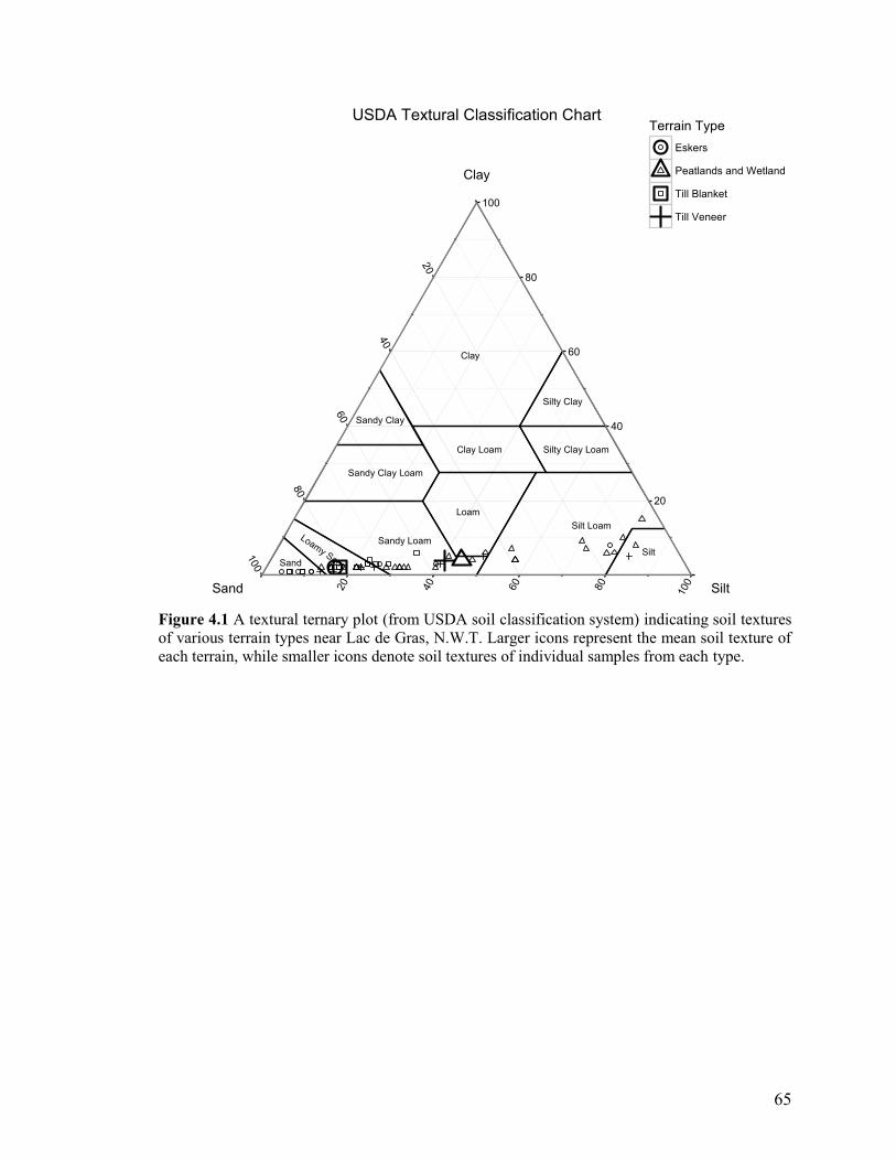
65
Figure 4.1 A textural ternary plot (from USDA soil classification system) indicating soil textures
of various terrain types near Lac de Gras, N.W.T. Larger icons represent the mean soil texture of
each terrain, while smaller icons denote soil textures of individual samples from each type.
Clay
Sandy Clay
Sandy Clay Loam
Sandy LoamLoam
y SandSand
Clay Loam
Loam
Silt Loam
Silty Clay
Silty Clay Loam
Silt
20
40
60
80
100
20
40
60
80
100
20
40
60
80
100
Clay
Sand Silt
Terrain Type
Eskers
Peatlands and Wetland
Till Blanket
Till Veneer
USDA Textural Classification Chart

66
for till blanket and eskers.
4.3. Depth Profiles: Moisture Content, Organic Matter and Soluble Cations
4.3.1. Moisture Content and Excess Ice Content
In peatlands and wetlands, water content GWB was usually high in samples
recorded as organics or ice-rich (Figure 4.2). “Till” samples generally had lower water
content GWB, but some tills with increased excess-ice contents in the near-surface
permafrost or at depth in permafrost had high water content GWB. The active layer at most
sites had high water contents. Similarly, water content GWB was also high (between 50
and 90%) in the near-surface permafrost. The zones with high water contents in the near-
surface permafrost were often associated with ice-lenses, several centimeters thick (Figure
4.2), but no excess ice was evident at the peatland sites (1005 and 1006), in the near-surface
permafrost. This is due to a very high organic matter content, over 75%, up to 1.5 m (Figure
4.2a and g). At most sites, water content GWB and excess ice contents at depth in
permafrost declined with depth (e.g. Figure 4.2a, b, d, e, and g), however some sites from
peatlands (1005 and 1009) were observed with increasing water content GWB and thick
ice lenses at depth with excess ice contents more than 50% (Figure 4.2c and f). These
ice-rich intervals corresponded with their respective sample types from the Unicode
information.

67
Figure 4.2 Gravimetric water content (GWB) and excess ice profiles from the active layer and
permafrost at peatlands and wetlands sites, near Lac de Gras, N.W.T. Blue triangles represent water
content GWB while dark blue upside down triangles represent excess ice content. The dashed line
represents the thickness of the active layer at the time of sampling while the dotted line represents
the lower boundary of the near-surface permafrost (See Figure 3.4 to 3.7 for location context).
a) 1006
Peatland
0.0
0.5
1.0
1.5
2.0
2.5
3.0
3.5
4.0
4.5
5.0
5.5
6.0
0 25 50 75 100 125
Depth
(m
)
Water Content GWB & Excess Ice (%)
b) 1007
Peatland
0.0
0.5
1.0
1.5
2.0
2.5
3.0
3.5
4.0
4.5
5.0
5.5
6.0
0 25 50 75 100 125
Depth
(m
)
Water Content GWB & Excess Ice (%)
c) 1005
Peatland
0.0
0.5
1.0
1.5
2.0
2.5
3.0
3.5
4.0
4.5
5.0
5.5
6.0
0 25 50 75 100 125
Depth
(m
)
Water Content GWB & Excess Ice (%)
d) 2011
Wetland
0.0
0.5
1.0
1.5
2.0
2.5
3.0
3.5
4.0
4.5
5.0
5.5
6.0
0 25 50 75 100 125
Depth
(m
)
Water Content GWB & Excess Ice (%)
e) 2012
Wetland
0.0
0.5
1.0
1.5
2.0
2.5
3.0
3.5
4.0
4.5
5.0
5.5
6.0
0 25 50 75 100 125
Depth
(m
)
Water Content GWB & Excess Ice (%)
f) 1009
Peatland
0.0
0.5
1.0
1.5
2.0
2.5
3.0
3.5
4.0
4.5
5.0
5.5
6.0
0 25 50 75 100 125
Depth
(m
)
Water Content GWB & Excess Ice (%)
g) 1010
Wetland
0.0
0.5
1.0
1.5
2.0
2.5
3.0
3.5
4.0
4.5
5.0
5.5
6.0
0 25 50 75 100 125
Depth
(m
)
Water Content GWB & Excess Ice (%)
h) 2015
Peatland
0.0
0.5
1.0
1.5
2.0
2.5
3.0
3.5
4.0
4.5
5.0
5.5
6.0
0 25 50 75 100 125
Depth
(m
)
Water Content GWB & Excess Ice (%)

68
At a few sites discrepancies existed between the active layer moisture contents
obtained between two exterior pits (Figure 4.2c and e), while some variations were also
observed between the water content GWB of boreholes and exterior pits in the active layer
(Figure 4.2f and g). Two sites in peatlands and wetlands terrain, i.e. 1009 and 1010, were
ice-rich from the base of the active layer to permafrost at depth with distinct zones of ice
lenses (Figure 4.2e, f, and g). These distinct zones of ice lenses had excess ice contents
between 25 and 60%.
In till blanket, a general correspondence in the water content profiles in the active
layer was observed between various sites (Figure 4.3). However, water content profiles
were different in the near-surface permafrost or at depth in permafrost depending upon the
local positions of boreholes in a hillslope. Most sites indicated a water content GWB of <
25% for the uppermost layer, with few exceptions at the hilltop and hillslope sites (2004,
2005 and 2007). Below this uppermost layer, lower moisture content extended to depths of
about 1.75 to 2 m at all sites. Similarly, no excess ice content was recorded at any site
except the hilltop site (2004) up to 2 m depth (Figure 4.3b). At this site (2004) two ice-rich
layers, 12 to 17 cm thick, with water content GWB between 14 and 20% were encountered
at 1.0 and 1.7 m depths. Similarly, another interval between 1.75 and 4.00 m depth was
underlain by three distinct ice-rich zones with water content GWB more than 60%. Excess
ice contents for all three intervals were more than 60%.
Sites located on steep slopes and bottom of hills also had excess ice, however they
were encountered much deeper in ground at the hill bottom site. Excess ice content was
present at 2.5 m depth at the steep slope (site 2007), however was absent for the same depth
interval at the bottom of the hill (site 2006) (Figure 4.3d and e).

69
Figure 4.3 Gravimetric water content (GWB) and excess ice profiles from the till blanket sites,
near Lac de Gras, N.W.T. Blue triangles represent water content GWB while dark blue upside down
triangles represent excess ice content. The dashed line represents the thickness of the active layer
at the time of sampling while the dotted line represents the lower boundary of the near-surface
permafrost (See Figure 3.4 to 3.7 for location context).
a) 1004
Hill 1 - Steep Slope
0.0
0.5
1.0
1.5
2.0
2.5
3.0
3.5
4.0
4.5
5.0
5.5
6.0
0 25 50 75 100 125
Dep
th (
m)
Water Content GWB & Excess Ice (%)
b) 2004
Hill 1 - Top of Hill
0.0
0.5
1.0
1.5
2.0
2.5
3.0
3.5
4.0
4.5
5.0
5.5
6.0
0 25 50 75 100 125
Dep
th (
m)
Water Content GWB & Excess Ice (%)
c) 2005
Hill 1 - Steep Slope
0.0
0.5
1.0
1.5
2.0
2.5
3.0
3.5
4.0
4.5
5.0
5.5
6.0
0 25 50 75 100 125
Dep
th (
m)
Water Content GWB & Excess Ice (%)
d) 2006
Hill 1 - Hill Bottom
0.0
0.5
1.0
1.5
2.0
2.5
3.0
3.5
4.0
4.5
5.0
5.5
6.0
0 25 50 75 100 125
De
pth
(m
)
Water Content GWB & Excess Ice (%)
e) 2007
Hill 1 - Steep Slope
0.0
0.5
1.0
1.5
2.0
2.5
3.0
3.5
4.0
4.5
5.0
5.5
6.0
0 25 50 75 100 125
De
pth
(m
)
Water Content GWB & Excess Ice (%)
f) 2033
Hill 3 - Top of Hill
0.0
0.5
1.0
1.5
2.0
2.5
3.0
3.5
4.0
4.5
5.0
5.5
6.0
0 25 50 75 100 125
De
pth
(m
)
Water Content GWB & Excess Ice (%)
g) 2009
Hill 3 - Hill Bottom
0.0
0.5
1.0
1.5
2.0
2.5
3.0
3.5
4.0
4.5
5.0
5.5
6.0
0 25 50 75 100 125
De
pth
(m
)
Water Content GWB & Excess Ice (%)
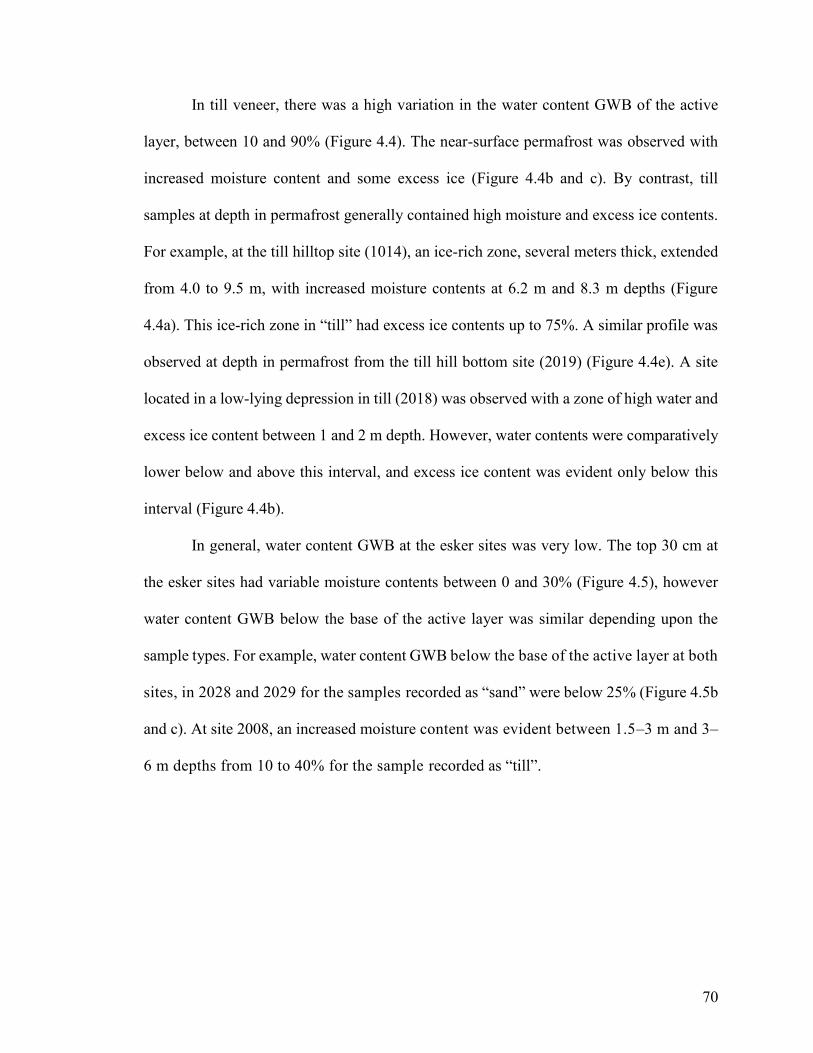
70
In till veneer, there was a high variation in the water content GWB of the active
layer, between 10 and 90% (Figure 4.4). The near-surface permafrost was observed with
increased moisture content and some excess ice (Figure 4.4b and c). By contrast, till
samples at depth in permafrost generally contained high moisture and excess ice contents.
For example, at the till hilltop site (1014), an ice-rich zone, several meters thick, extended
from 4.0 to 9.5 m, with increased moisture contents at 6.2 m and 8.3 m depths (Figure
4.4a). This ice-rich zone in “till” had excess ice contents up to 75%. A similar profile was
observed at depth in permafrost from the till hill bottom site (2019) (Figure 4.4e). A site
located in a low-lying depression in till (2018) was observed with a zone of high water and
excess ice content between 1 and 2 m depth. However, water contents were comparatively
lower below and above this interval, and excess ice content was evident only below this
interval (Figure 4.4b).
In general, water content GWB at the esker sites was very low. The top 30 cm at
the esker sites had variable moisture contents between 0 and 30% (Figure 4.5), however
water content GWB below the base of the active layer was similar depending upon the
sample types. For example, water content GWB below the base of the active layer at both
sites, in 2028 and 2029 for the samples recorded as “sand” were below 25% (Figure 4.5b
and c). At site 2008, an increased moisture content was evident between 1.5–3 m and 3–
6 m depths from 10 to 40% for the sample recorded as “till”.

71
Figure 4.4 Gravimetric water content (GWB) and excess ice profiles from the active layer and
permafrost, till veneer sites, near Lac de Gras, N.W.T. Blue triangles represent water content GWB
while dark blue upside down triangles represent excess ice content. The dashed line represents the
thickness of the active layer at the time of sampling while the dotted line represents the lower
boundary of the near-surface permafrost (See Figure 3.4 to 3.7 for location context).
a) 1014
Hill 2 - Top of Hill
0
1
2
3
4
5
6
7
8
9
10
0 25 50 75 100 125
De
pth
(m
)
Water Content GWB & Excess Ice (%)
b) 2018
Hill 2 - Low-lying Depression
0
1
2
3
4
5
6
7
8
9
10
0 25 50 75 100 125D
ep
th (
m)
Water Content GWB & Excess Ice (%)
c) 2013
Hill Bottom (Snow Drifts)
0
1
2
3
4
5
6
7
8
9
10
0 25 50 75 100 125
De
pth
(m
)
Water Content GWB & Excess Ice (%)
d) 2016
Hill Bottom
0
1
2
3
4
5
6
7
8
9
10
0 25 50 75 100 125
Dep
th (
m)
Water Content GWB & Excess Ice (%)
e) 2019
Hill Bottom (Snow Drifts)
0
1
2
3
4
5
6
7
8
9
10
0 25 50 75 100 125
Dep
th (
m)
Water Content GWB & Excess Ice (%)

72
Figure 4.5 Gravimetric water content (GWB) profiles from the esker sites, near Lac de Gras,
N.W.T. The dashed line represents the thickness of the active layer at the time of sampling while
the dotted line represents the lower boundary of the near-surface permafrost (See Figure 3.4 to 3.7
for location context).
a) 2008
0
1
2
3
4
5
6
7
8
9
10
11
12
0 25 50 75 100 125
De
pth
(m
)
Water Content GWB (%)
b) 2028
0
1
2
3
4
5
6
7
8
9
10
11
12
0 25 50 75 100 125
De
pth
(m
)
Water Content GWB (%)
c) 2029
0
1
2
3
4
5
6
7
8
9
10
11
12
0 25 50 75 100 125
De
pth
(m
)
Water Content GWB (%)
d) 2026
0
1
2
3
4
5
6
7
8
9
10
11
12
0 25 50 75 100 125
De
pth
(m
)
Water Content GWB (%)

73
4.3.2. Organic Matter Content
In peatlands and wetlands, the organic matter content in the active layer and in near-
surface permafrost of few sites was very high, up to 90% (Figure 4.6a, c and g), and
corresponded to their respective sample types. Organic matter contents normally declined
with depth, and were the lowest at depth in permafrost. However, at one peatland site
(1006) organic matter between 1.5 m and 2.5 m depth was very high, about 85% (Figure
4.6a). The majority of “till” samples in profiles were observed to have low organic matter
contents (Figure 4.6c). By contrast, organic matter contents were also associated with ice-
rich samples at depth in permafrost with some minor increments (Figure 4.6c and f),
however the absolute percentage of this organic content at depth was very low.
In till blanket, the organic matter content of the top 50 cm depth was less than 5%
at each site (Figure 4.7). In comparison to peatlands and wetlands terrain, this percentage
of organic content in the active layer is low, which is likely due to the surface condition
and vegetation. This is reflected in observed sample types of till blanket terrain in the
uppermost layer, which were mostly classified as “till”. Some minor increments in organic
matter contents were noticed near the base of the active layer at the steep slope site (1004)
and the hill bottom site (2006) (Figure 4.7a and d), however organics in the soil profile
declined in cores at site from the top of the hill (2004) (Figure 4.7b). The near-surface
permafrost in till blanket terrain contained only 2 to 5% of organic matter, and was quite
comparable with the organic matter in the active layer. Organic matter content at depth in
permafrost was generally low, less than 2.5%, but some minor increments were observed at
depth for sites located at the hilltop (2004) and the steep slope (2007) (Figure 4.7b and e).

74
Figure 4.6 Soil Organic-matter contents in the active layer and permafrost, peatlands and wetlands
site, near Lac de Gras, N.W.T. The dashed line represents the represents the thickness of the active
layer at the time of sampling while the dotted line represents the lower boundary of the near-surface
permafrost (See Figure 3.4 to 3.7 for location context).
a) 1006
Peatland
0.0
0.5
1.0
1.5
2.0
2.5
3.0
3.5
4.0
4.5
5.0
5.5
6.0
0 25 50 75 100 125
Dep
th (
m)
Organic Matter GDB (%)
b) 1007
Peatland
0.0
0.5
1.0
1.5
2.0
2.5
3.0
3.5
4.0
4.5
5.0
5.5
6.0
0 25 50 75 100 125
Dep
th (
m)
Organic Matter GDB (%)
c) 1005
Peatland
0.0
0.5
1.0
1.5
2.0
2.5
3.0
3.5
4.0
4.5
5.0
5.5
6.0
0 25 50 75 100 125
Dep
th (
m)
Organic Matter GDB (%)
d) 2011
Wetland
0.0
0.5
1.0
1.5
2.0
2.5
3.0
3.5
4.0
4.5
5.0
5.5
6.0
0 25 50 75 100 125
Dep
th (
m)
Organic Matter GDB (%)
e) 2012
Wetland
0.0
0.5
1.0
1.5
2.0
2.5
3.0
3.5
4.0
4.5
5.0
5.5
6.0
0 25 50 75 100 125
Depth
(m
)
Organic Matter GDB (%)
f) 1009
Peatland
0.0
0.5
1.0
1.5
2.0
2.5
3.0
3.5
4.0
4.5
5.0
5.5
6.0
0 25 50 75 100 125
Depth
(m
)
Organic Matter GDB (%)
g) 1010
Wetland
0.0
0.5
1.0
1.5
2.0
2.5
3.0
3.5
4.0
4.5
5.0
5.5
6.0
0 25 50 75 100 125
Depth
(m
)
Organic Matter GDB (%)
h) 2015
Peatland
0.0
0.5
1.0
1.5
2.0
2.5
3.0
3.5
4.0
4.5
5.0
5.5
6.0
0 25 50 75 100 125
Depth
(m
)
Organic Matter GDB (%)
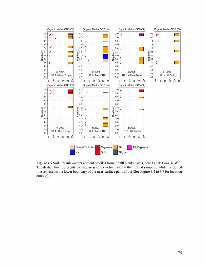
75
Figure 4.7 Soil Organic-matter content profiles from the till blanket sites, near Lac de Gras, N.W.T.
The dashed line represents the thickness of the active layer at the time of sampling while the dotted
line represents the lower boundary of the near-surface permafrost (See Figure 3.4 to 3.7 for location
context).
a) 1004
Hill 1 - Steep Slope
0.0
0.5
1.0
1.5
2.0
2.5
3.0
3.5
4.0
4.5
5.0
5.5
6.0
0 5 10 15 20 25
Depth
(m
)
Organic Matter GDB (%)
b) 2004
Hill 1 - Top of Hill
0.0
0.5
1.0
1.5
2.0
2.5
3.0
3.5
4.0
4.5
5.0
5.5
6.0
0 5 10 15 20 25
Depth
(m
)
Organic Matter GDB (%)
c) 2005
Hill 1 - Steep Slope
0.0
0.5
1.0
1.5
2.0
2.5
3.0
3.5
4.0
4.5
5.0
5.5
6.0
0 5 10 15 20 25
Depth
(m
)
Organic Matter GDB (%)
d) 2006
Hill 1 - Hill Bottom
0.0
0.5
1.0
1.5
2.0
2.5
3.0
3.5
4.0
4.5
5.0
5.5
6.0
0 5 10 15 20 25
Depth
(m
)
Organic Matter GDB (%)
e) 2007
Hill 1 - Steep Slope
0.0
0.5
1.0
1.5
2.0
2.5
3.0
3.5
4.0
4.5
5.0
5.5
6.0
0 5 10 15 20 25
Depth
(m
)
Organic Matter GDB (%)
f) 2033
Hill 3 - Top of Hill
0.0
0.5
1.0
1.5
2.0
2.5
3.0
3.5
4.0
4.5
5.0
5.5
6.0
0 5 10 15 20 25
Depth
(m
)
Organic Matter GDB (%)
g) 2009
Hill 3 - Hill Bottom
0.0
0.5
1.0
1.5
2.0
2.5
3.0
3.5
4.0
4.5
5.0
5.5
6.0
0 5 10 15 20 25
Depth
(m
)
Organic Matter GDB (%)

76
In till veneer, organic matter content at depth in permafrost was generally low, less
than 1.5% as observed at the till hilltop and hill bottom sites (1014, 2013 and 2019) (Figure
4.8a, c and e). The majority of samples at depth from this terrain were associated with “till”
of varying excess ice contents. Similarly, organic matter content in the active layer was
also low, between 2 and 6%, however in the near-surface permafrost was high, about 65%
(Figure 4.8b and d).
At the esker sites, the top 50 cm depth was characterized with organic matter
contents between 1 and 6%, and was quite similar among most sites (Figure 4.9a, c and d).
In the near-surface permafrost and at depth in permafrost, organic matter content was
generally low and the profiles were relatively similar to each other. The observed relatively
high percentage of organic matter in the active layer, and low percentage at depth
corresponded with the sample nature belonging to those depths.
4.3.3. Total Soluble Cations
In peatlands and wetlands, total soluble cation concentration in the active layer had
a wide variation, between 0.72 to 3.43 meq/100 g (Table 4.1). Similarly, the near-surface
permafrost at some sites was observed with increased concentrations. The mean total
soluble cation concentration in the active layer was at least 5 times greater than that present
in the near-surface permafrost (Table 4.1). Permafrost at depth generally contained low
soluble cation concentrations, however some minor peaks were evident in ice-rich samples.
The majority of “organic” samples in profiles from the active layer and near-
surface permafrost contained high soluble cation concentrations (Figure 4.10a, c and g).
“Till” samples normally contained low soluble cations, but a few sites at depth were

77
Figure 4.8 Soil Organic-matter contents in the active layer and permafrost, till veneer sites, near
Lac de Gras, N.W.T. The dashed line represents the thickness of the active layer at the time of
sampling while the dotted line represents the lower boundary of the near-surface permafrost (See
Figure 3.4 to 3.7 for location context).
a) 1014
Hill 2 - Top of Hill
0
1
2
3
4
5
6
7
8
9
10
0 25 50 75 100 125
Depth
(m
)
Organic Matter GDB (%)
b) 2018
Hill 2 - Low-lying Depression
0
1
2
3
4
5
6
7
8
9
10
0 25 50 75 100 125
Depth
(m
)
Organic Matter GDB (%)
c) 2013
Hill Bottom (Snow Drifts)
0
1
2
3
4
5
6
7
8
9
10
0 25 50 75 100 125
Depth
(m
)
Organic Matter GDB (%)
d) 2016
Hill Bottom
0
1
2
3
4
5
6
7
8
9
10
0 25 50 75 100 125
Depth
(m
)
Organic Matter GDB (%)
e) 2019
Hill Bottom (Snow Drifts)
0
1
2
3
4
5
6
7
8
9
10
0 25 50 75 100 125
Depth
(m
)
Organic Matter GDB (%)

78
Figure 4.9 Soil Organic-matter content profiles from the esker sites, near Lac de Gras, N.W.T. The
dashed line represents the thickness of the active layer at the time of sampling while the dotted line
represents the lower boundary of the near-surface permafrost (See Figure 3.4 to 3.7 for location
context).
a) 2008
0
1
2
3
4
5
6
7
8
9
10
11
12
0 20 40 60
De
pth
(m
)
Organic Matter GDB (%)
b) 2028
0
1
2
3
4
5
6
7
8
9
10
11
12
0 20 40 60
De
pth
(m
)
Organic Matter GDB (%)
c) 2029
0
1
2
3
4
5
6
7
8
9
10
11
12
0 20 40 60
De
pth
(m
)
Organic Matter GDB (%)
d) 2026
0
1
2
3
4
5
6
7
8
9
10
11
12
0 20 40 60
De
pth
(m
)
Organic Matter GDB (%)

79
observed with increased concentrations, about 3 meq/100 g (Figure 4.10d and f). The top
of the permafrost at a few sites was observed with an increased soluble cation concentration
compared to that at the base of the active layer. For example, at the peatland site (1006),
total soluble cation concentration increased from 2.16 meq/100 g at the base of the active
layer to 3.16 meq/100 g in a moisture enriched zone in near-surface permafrost (Figure
4.2a and 4.10a). Similar patterns were also observed at the peatland and wetland sites (1005
and 1010) (Figure 4.10c and g). All three sites had high organic matter content in the active
layer and in the near-surface permafrost (Figure 4.6a, c and g). Soluble cation concentration
also increased at depth in permafrost. For example, at one wetland site (2011) the depth
interval between 2 m and 3 m depth was observed with an increased concentration of
soluble cations up to 3 meq/100 g dry soil (Figure 4.10d).
The enriched zones in soluble cations at the majority of sites correspond with the
ice-rich zones at that particular depth. Zones of low cation concentration also coincided
with low ice contents in permafrost. For example, similar patterns in ice and soluble ion
accumulation were observed at depth in profiles from the peatland and wetland sites (1005
and 1010) underlain by high-ice-content permafrost (Figure 4.2c and 4.10c). However, at
the wetland site (2011), the depth just below the base of the active layer was characterized
by very low soluble cation concentration, and the zone of high cation concentration
coincided with low ice content at the top of permafrost (Figure 4.10d and 4.2d).
In peatlands and wetlands, Mg2+ was the dominant cation reported from the active
layer and permafrost at most sites except at the two peatland sites (1006 and 2015). At
these two sites, the concentration of soluble Mg2+ in the active layer was slightly less than
soluble Ca2+ (Table 4.1). The highest concentration of Mg2+ in the active layer was reported

80
Figure 4.10 Profiles of total soluble cations in the active layer and permafrost, peatlands and
wetlands sites, near Lac de Gras, N.W.T. The dashed line represents the thickness of the active
layer at the time of sampling while the dotted line represents the inferred depth of the near-surface
permafrost while the dotted line represents the lower boundary of the near-surface permafrost (See
Figure 3.4 to 3.7 for location context).
a) 1006
Peatland
0.0
0.5
1.0
1.5
2.0
2.5
3.0
3.5
4.0
4.5
5.0
5.5
6.0
0 2 4 6
Depth
(m
)
Total Soluble Cations (meq/100g dry soil)
b) 1007
Peatland
0.0
0.5
1.0
1.5
2.0
2.5
3.0
3.5
4.0
4.5
5.0
5.5
6.0
0 2 4 6
Depth
(m
)
Total Soluble Cations (meq/100g dry soil)
c) 1005
Peatland
0.0
0.5
1.0
1.5
2.0
2.5
3.0
3.5
4.0
4.5
5.0
5.5
6.0
0 2 4 6
Depth
(m
)
Total Soluble Cations (meq/100g dry soil)
d) 2011
Wetland
0.0
0.5
1.0
1.5
2.0
2.5
3.0
3.5
4.0
4.5
5.0
5.5
6.0
0 2 4 6
Depth
(m
)
Total Soluble Cations (meq/100g dry soil)
e) 2012
Wetland
0.0
0.5
1.0
1.5
2.0
2.5
3.0
3.5
4.0
4.5
5.0
5.5
6.0
0 2 4 6
Depth
(m
)
Total Soluble Cations (meq/100g dry soil)
f) 1009
Peatland
0.0
0.5
1.0
1.5
2.0
2.5
3.0
3.5
4.0
4.5
5.0
5.5
6.0
0 2 4 6
Depth
(m
)
Total Soluble Cations (meq/100g dry soil)
g) 1010
Wetland
0.0
0.5
1.0
1.5
2.0
2.5
3.0
3.5
4.0
4.5
5.0
5.5
6.0
0 2 4 6
Depth
(m
)
Total Soluble Cations (meq/100g dry soil)
h) 2015
Peatland
0.0
0.5
1.0
1.5
2.0
2.5
3.0
3.5
4.0
4.5
5.0
5.5
6.0
0 2 4 6
Depth
(m
)
Total Soluble Cations (meq/100g dry soil)

81
Table 4.1 Mean total soluble cation concentrations of various sites located within the
peatlands and wetlands sites
Mean Total Soluble cations (meq/ 100g dry soil)
Borehole ID
(NGO-DD15-
Active Layer Permafrost
Ca2+ Mg2+ K+ Na+ Total Ca2+ Mg2+ K+ Na+ Total
1006 0.49 0.42 0.15 0.11 1.18 0.66 0.59 0.07 0.16 1.48
1007 0.24 0.36 0.23 0.12 0.95 0.01 0.02 0.01 0.02 0.05
1005 0.20 0.25 0.15 0.11 0.72 0.33 0.34 0.10 0.11 0.88
2011 1.04 1.39 0.68 0.33 3.43 0.22 0.39 0.03 0.07 0.72
2012 0.23 0.32 0.25 0.07 0.87 0.05 0.09 0.01 0.03 0.17
1009 0.78 0.90 0.31 0.30 2.29 0.31 0.58 0.05 0.14 1.07
1010 0.82 0.97 0.64 0.24 2.67 0.17 0.30 0.03 0.07 0.57
Top 1 m depth (unfrozen) Below 1 m depth (frozen)
2015 0.08 0.07 0.01 0.03 0.19 0.03 0.04 0.00 0.06 0.14

82
from the wetland site (2011) with 1.39 meq/100g, while in permafrost it was measured at
the peatland site (1006) with 0.59 meq/100 g (Table 4.1). Similarly, Ca2+ was the other
soluble cation whose relative abundance was quite high especially at the wetland sites
(1010 and 2011), and one peatland site (1009) (Table 4.1). The concentrations of soluble
K+ and Na+ were high in the active layer, but in permafrost they were relatively low (Table
4.1). In absolute terms, the concentration of soluble Na+ was the lowest in the active
layer at only two peatland sites, whereas in permafrost, soluble K+ was recorded with their
lowest concentrations at all sites (Table 4.1).
In till blanket, total soluble cation concentration of the active layer was generally
low except at few sites from the top of the hill and steep slopes (2004, 2005 and 2007)
(Figure 4.11b, c and e). At these three sites, soluble cation concentrations of the topmost
layer between 0 and 10 cm depth were much higher, and declined with the elevation from
the top of the hill down the steep slope, to the lowest at the bottom of the hill (Figure 4.11d).
These variations in cation concentrations of the active layer along a hillslope correspond
to the processes explained in Section 2.4.2.2 and Figure 2.6, on how geochemical
conditions vary between depositional and erosive permafrost environments. The same
phenomenon however could not be explained with the data obtained from Hill 3 as the
active layer consisted of relatively low concentrations, both at the top of the hill as well as
the hill bottom (Figure 4.11f and g).
Mean total soluble cation concentrations of the top 1 m and the ground below it
indicated that four of seven sites were enriched with higher soluble cation concentrations
in permafrost than in the active layer in till blanket terrain (Table 4.2). The mean
concentration of cations in permafrost was very low, between 0.22 to 0.50 meq/100 g.
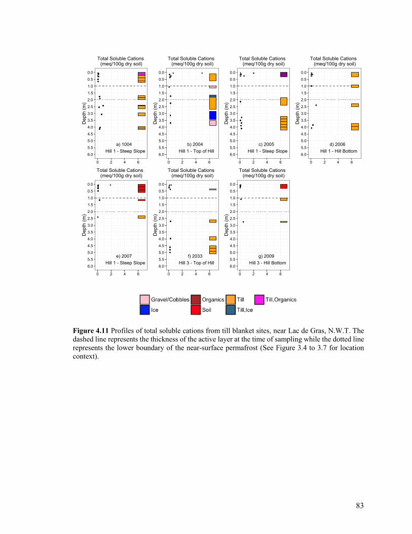
83
Figure 4.11 Profiles of total soluble cations from till blanket sites, near Lac de Gras, N.W.T. The
dashed line represents the thickness of the active layer at the time of sampling while the dotted line
represents the lower boundary of the near-surface permafrost (See Figure 3.4 to 3.7 for location
context).
a) 1004
Hill 1 - Steep Slope
0.0
0.5
1.0
1.5
2.0
2.5
3.0
3.5
4.0
4.5
5.0
5.5
6.0
0 2 4 6
Depth
(m
)
Total Soluble Cations (meq/100g dry soil)
b) 2004
Hill 1 - Top of Hill
0.0
0.5
1.0
1.5
2.0
2.5
3.0
3.5
4.0
4.5
5.0
5.5
6.0
0 2 4 6
Depth
(m
)
Total Soluble Cations (meq/100g dry soil)
c) 2005
Hill 1 - Steep Slope
0.0
0.5
1.0
1.5
2.0
2.5
3.0
3.5
4.0
4.5
5.0
5.5
6.0
0 2 4 6
Depth
(m
)
Total Soluble Cations (meq/100g dry soil)
d) 2006
Hill 1 - Hill Bottom
0.0
0.5
1.0
1.5
2.0
2.5
3.0
3.5
4.0
4.5
5.0
5.5
6.0
0 2 4 6
Depth
(m
)
Total Soluble Cations (meq/100g dry soil)
e) 2007
Hill 1 - Steep Slope
0.0
0.5
1.0
1.5
2.0
2.5
3.0
3.5
4.0
4.5
5.0
5.5
6.0
0 2 4 6
Depth
(m
)
Total Soluble Cations (meq/100g dry soil)
f) 2033
Hill 3 - Top of Hill
0.0
0.5
1.0
1.5
2.0
2.5
3.0
3.5
4.0
4.5
5.0
5.5
6.0
0 2 4 6
Depth
(m
)
Total Soluble Cations (meq/100g dry soil)
g) 2009
Hill 3 - Hill Bottom
0.0
0.5
1.0
1.5
2.0
2.5
3.0
3.5
4.0
4.5
5.0
5.5
6.0
0 2 4 6
Depth
(m
)
Total Soluble Cations (meq/100g dry soil)

84
Table 4.2 Mean total soluble cation concentrations of various sites located within the till
blanket sites
Mean Total Soluble cations (meq/ 100g dry soil)
Borehole ID
(NGO-DD15-
Top 1 m depth (unfrozen) Below 1 m depth (frozen)
Ca2+ Mg2+ K+ Na+ Total Ca2+ Mg2+ K+ Na+ Total
1004 0.03 0.02 0.01 0.03 0.08 0.10 0.12 0.07 0.08 0.37
2004 0.27 0.45 0.20 0.03 0.94 0.06 0.11 0.03 0.02 0.23
2005 0.16 0.19 0.09 0.03 0.47 0.06 0.07 0.04 0.03 0.18
2006 0.03 0.03 0.01 0.02 0.08 0.11 0.13 0.03 0.03 0.30
2033 0.05 0.06 0.01 0.02 0.14 0.06 0.09 0.04 0.03 0.22
2007 0.09 0.10 0.06 0.03 0.29 0.01 0.01 0.01 0.01 0.04
2009 0.02 0.03 0.01 0.02 0.08 0.15 0.24 0.07 0.04 0.50

85
However, mean total soluble cation concentration in the top 1 m depth was recorded up to
0.94 meq/100 g at the hilltop site (2004) (Table 4.2).
In till blanket, soluble cation concentrations at depth in permafrost of few sites
increased to more than double those present at the near-surface permafrost (Figure 4.11a,
d and g). For example, at the till steep slope site (1004), an increase in the concentration
from 0.33 meq/100 g to 0.80 meq/100 g was evident between the depths of 2.0 and 2.5
m. At the hill bottom sites (2006 and 2009), a similar increase in cation concentration was
observed at depths of around 2.5 m where soluble cations reached up to 0.77 meq/100 g
(Figure 4.11d and 4.11g).
In till blanket, Mg2+ was the dominant cation reported from the top 1 m and below
1 m depth at most sites (Table 4.2). Similarly, Ca2+ was also available in comparable
amounts, but the absolute concentrations of both ions were low, not more than 0.45
meq/100 g (Table 4.2). Furthermore, soluble K+ and Na+ were also detected, and the
relative abundances of these two ions were quite comparable with other cations, especially
from the permafrost.
In till veneer, active layer soluble cation concentrations at the low-lying hill bottom
sites (2018 and 2019) were comparatively higher than those at depths in permafrost (Figure
4.12b and e). At the low-lying depression site (2018), mean total soluble cation
concentrations of the active layer reached up to 0.90 meq/100 g, while in permafrost was
only about 0.25 meq/100 g (Table 4.3). Similarly, at the hill bottom site (2019) mean total
soluble cation concentrations in the active layer was nearly double those in permafrost
(Table 4.3). The high concentrations of soluble cations at the topmost layers of these sites
were mostly related to the organic samples.

86
Figure 4.12 Profiles of total soluble cations in the active layer and permafrost, till veneer sites,
near Lac de Gras, N.W.T. The dashed line represents the thickness of the active layer at the time
of sampling while the dotted line represents the lower boundary of the near-surface permafrost (See
Figure 3.4 to 3.7 for location context).
a) 1014
Hill 2 - Top of Hill
0
1
2
3
4
5
6
7
8
9
10
0 2 4 6
Depth
(m
)
Total Soluble Cations (meq/100g dry soil)
b) 2018
Hill 2 - Low-lying Depression
0
1
2
3
4
5
6
7
8
9
10
0 2 4 6
Depth
(m
)
Total Soluble Cations (meq/100g dry soil)
c) 2013
Hill Bottom (Snow Drifts)
0
1
2
3
4
5
6
7
8
9
10
0 2 4 6
Depth
(m
)
Total Soluble Cations (meq/100g dry soil)
d) 2016
Hill Bottom
0
1
2
3
4
5
6
7
8
9
10
0 2 4 6
Depth
(m
)
Total Soluble Cations (meq/100g dry soil)
e) 2019
Hill Bottom (Snow Drifts)
0
1
2
3
4
5
6
7
8
9
10
0 2 4 6
Depth
(m
)
Total Soluble Cations (meq/100g dry soil)

87
Table 4.3 Mean total soluble cation concentrations of various sites located within the till
veneer sites
Mean Total Soluble cations (meq/ 100g dry soil)
Borehole ID
(NGO-DD15-
Active Layer Permafrost
Ca2+ Mg2+ K+ Na+ Total Ca2+ Mg2+ K+ Na+ Total
2018 0.28 0.34 0.09 0.19 0.90 0.09 0.11 0.01 0.03 0.25
2019 0.15 0.14 0.11 0.05 0.45 0.06 0.13 0.01 0.05 0.25
Top 1 m depth (unfrozen) Below 1 m depth (frozen)
1014 N/A N/A N/A N/A N/A 0.13 0.16 0.07 0.04 0.39
2013 0.06 0.09 0.13 0.04 0.32 0.45 0.83 0.02 0.09 1.39
2016 0.06 0.06 0.02 0.03 0.17 0 0 0 0 0

88
Few sites also contained high soluble cation concentrations at depth in permafrost
(Figure 4.12a and c). For example, at the hilltop site (1014), total soluble cation
concentrations at depth between 4.0 m and 9.5 m ranged between 0.06 to 1.04 meq/100 g,
and fluctuations mostly followed the ice-rich intervals (Figure 4.12a and Figure 4.4a).
However, this was not true at the hill bottom site (2013) (Figure 4.12c and Figure 4.4c).
The depth interval between 2.0 m and 2.5 m contained high concentration of soluble
cations, greater than 1.1 meq/100 g, but the excess ice contents at this depth interval were
much lower.
In till veneer, Mg2+ was the dominant cation reported from the permafrost at all
sites. The concentration of soluble Mg2+ in permafrost ranged between 0.11 to 0.83
meq/100 g (Table 4.3). In the active layer, Mg2+ was a dominant cation at only two sites in
2018 and 2019 (Table 4.3). At other sites, active layer soluble cation concentration was
either dominated by Ca2+ ions or the relative abundance of Ca2+ was comparable with
soluble Mg2+ ions. Similarly, soluble K+ and Na+ were also present in considerable amounts
within the active layer at till veneer sites, but the relative abundances of these ions in
permafrost was comparatively low (Table 4.3).
At the esker sites, the relative and absolute concentrations of total soluble cations
in the active layer and in permafrost were very low (Figure 4.13). A comparison of mean
total soluble cation concentrations indicated that permafrost had higher soluble cation
concentrations than the active layer (Table 4.4). Most sites in eskers indicated very low
total soluble cation concentration of less than 0.25 meq/100 g except at 2028. At this

89
Figure 4.13 Profiles of total soluble cations from the esker sites, near Lac de Gras, N.W.T. The
dashed line represents the thickness of the active layer at the time of sampling while the dotted line
represents the lower boundary of the near-surface permafrost (See Figure 3.4 to 3.7 for location
context).
a) 2008
0
1
2
3
4
5
6
7
8
9
10
11
12
0.0 0.5 1.0 1.5 2.0 2.5
Dep
th (
m)
Total Soluble Cations (meq/100g dry soil)
b) 2028
0
1
2
3
4
5
6
7
8
9
10
11
12
0.0 0.5 1.0 1.5 2.0 2.5
Dep
th (
m)
Total Soluble Cations (meq/100g dry soil)
c) 2029
0
1
2
3
4
5
6
7
8
9
10
11
12
0.0 0.5 1.0 1.5 2.0 2.5
De
pth
(m
)
Total Soluble Cations (meq/100g dry soil)
d) 2026
0
1
2
3
4
5
6
7
8
9
10
11
12
0.0 0.5 1.0 1.5 2.0 2.5
De
pth
(m
)
Total Soluble Cations (meq/100g dry soil)

90
Table 4.4 Mean total soluble cation concentrations of various sites located within the
esker sites
Mean Total Soluble cations (meq/ 100g dry soil)
Borehole ID
(NGO-DD15-
Top 50 cm depth (unfrozen) Below 50 cm depth (frozen)
Ca2+ Mg2+ K+ Na+ Total Ca2+ Mg2+ K+ Na+ Total
2026 0.03 0.03 0.01 0.02 0.08 0.03 0.05 0.02 0.03 0.13
Top 1 m depth (unfrozen) Below 1 m depth (frozen)
2008 0.01 0.02 0.01 0.01 0.05 0.01 0.01 0.02 0.04 0.10
2028 0.01 0.04 0.02 0.01 0.09 0.05 0.08 0.07 0.11 0.31
2029 0.01 0.00 0.00 0.01 0.02 0.01 0.01 0.02 0.05 0.08
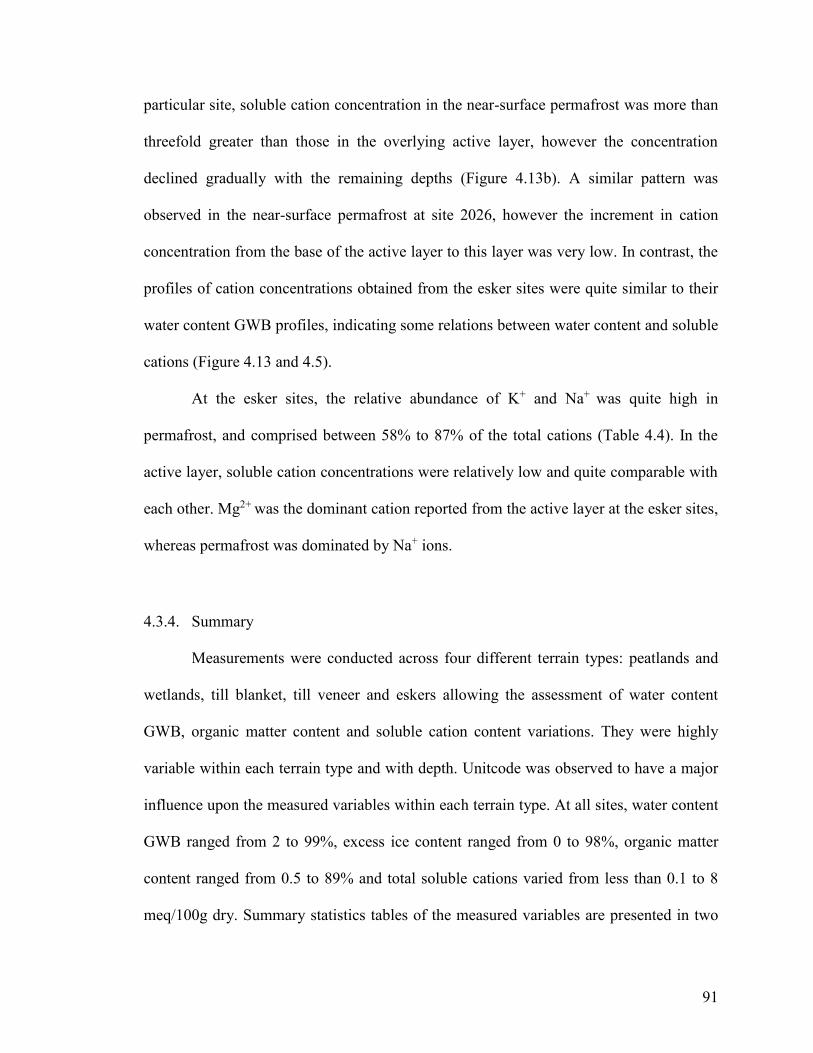
91
particular site, soluble cation concentration in the near-surface permafrost was more than
threefold greater than those in the overlying active layer, however the concentration
declined gradually with the remaining depths (Figure 4.13b). A similar pattern was
observed in the near-surface permafrost at site 2026, however the increment in cation
concentration from the base of the active layer to this layer was very low. In contrast, the
profiles of cation concentrations obtained from the esker sites were quite similar to their
water content GWB profiles, indicating some relations between water content and soluble
cations (Figure 4.13 and 4.5).
At the esker sites, the relative abundance of K+ and Na+ was quite high in
permafrost, and comprised between 58% to 87% of the total cations (Table 4.4). In the
active layer, soluble cation concentrations were relatively low and quite comparable with
each other. Mg2+ was the dominant cation reported from the active layer at the esker sites,
whereas permafrost was dominated by Na+ ions.
4.3.4. Summary
Measurements were conducted across four different terrain types: peatlands and
wetlands, till blanket, till veneer and eskers allowing the assessment of water content
GWB, organic matter content and soluble cation content variations. They were highly
variable within each terrain type and with depth. Unitcode was observed to have a major
influence upon the measured variables within each terrain type. At all sites, water content
GWB ranged from 2 to 99%, excess ice content ranged from 0 to 98%, organic matter
content ranged from 0.5 to 89% and total soluble cations varied from less than 0.1 to 8
meq/100g dry. Summary statistics tables of the measured variables are presented in two

92
different ways – (1) with respect to depth, integrating from the surface + the depths of 0.5
m, 1 m, 2 m, 4 m, 6 m and 10 m (Appendix F), and (2) with respect to strata, i.e., in the
active layer, near-surface permafrost and at depth in permafrost (Tables 4.5, 4.6 and 4.7).
In comparing variations with respect to depth and sites statistically, the number of
sample (N) and actual percentage sampled (PS) were the limiting factors in the near-surface
permafrost and also at depth in permafrost. PS is the actual interval sampled from the active
layer, near-surface permafrost or from the permafrost at depth expressed as a percentage
of the total thickness of that layer. N and PS were extremely low in the active layer of some
sites for the organic matter content. Thus, variations with respect to depth are presented
graphically with plots for describing the absolute amounts of water, organic matter and
soluble cations at different depths.
4.3.4.1. Gravimetric Water Content (%) Variations
Gravimetric water content was highly variable between depths for all terrain types
except the eskers (Figure 4.14A). Similarly, water content GWB also varied between
terrain types, and was observed to be the lowest at the esker sites. The highest water content
GWB values were associated with the active layers in peatlands and wetlands with the
median of 83%, which is due to wet conditions and high organic matter in the uppermost
layers of those sites. Till blanket and till veneer contained lower water contents in the active
layer. A few sites from peatlands and wetlands, and till veneer have high median water
contents GWB in the near-surface permafrost (Figure 4.14A). Water content GWB at depth
in permafrost was also high, and were quite similar between two terrains (peatlands and
wetlands and till veneer) with median of about 40%, whereas in till blanket it was much higher

93
Table 4.5 and Table 4.6: Summary statistics of gravimetric water content GWB (%) and organic matter content GDB (%) in the active layer, near-surface permafrost and at depth in
permafrost of 24 sites near Lac de Gras, N.W.T. N is the number of samples, PS (%) is the percentage of total sampling that was considered and N/A values delineate depth intervals where
no samples were recovered or core lengths that did not reach the specified depths.
4.5. GWB Active Layer Near-Surface Permafrost Permafrost Depth
Terrain Core ID
N
PS
(%) Mean Median Max Min SD
N
PS
(%) Mean Median Max Min SD
N Mean Median Max Min SD
Peatlands and wetlands 1006 7 100 81.3 80.9 89.3 78.0 3.8 4 90 85.8 85.9 88.6 82.8 2.5 7 48.5 32.7 84.4 11.6 32.7
1007 6 86 84.2 84.9 86.8 80.0 2.6 3 60 42.0 40.8 52.3 33.0 9.7 11 21.8 9.8 61.8 5.2 21.0
1005 6 86 59.7 83.2 85.3 10.6 37.8 6 93 55.3 63.7 81.9 14.9 25.5 14 55.5 49.5 98.7 11.6 32.1
2011 6 100 90.4 90.6 92.1 87.6 1.6 4 75 43.6 45.4 55.8 27.7 14.0 20 28.3 22.5 54.1 19.2 11.5
2012 6 55 43.8 42.4 76.1 17.4 28.4 2 48 35.8 35.8 42.2 29.3 9.2 10 41.2 44.2 52.5 13.2 12.0
1009 7 83 81.3 82.2 91.1 59.5 10.8 3 79 55.9 48.1 73.7 45.8 15.5 11 56.9 53.7 65.5 45.9 6.4
1010 8 100 77.7 84.7 92.8 45.9 16.9 3 72 63.5 59.3 76.8 54.4 11.8 16 45.2 41.7 71.7 30.3 11.0
2015 6 30 20.4 17.9 31.8 16.4 5.9 5 100 39.5 34.1 53.2 29.3 11.5 0 N/A N/A N/A N/A N/A
Till Blanket 1004 10 74 7.9 8.4 10.5 4.1 2.2 2 31 8.0 8.0 9.3 6.7 1.9 5 13.2 12.9 25.9 6.3 7.8
2004 7 60 23.3 14.7 68.2 8.7 22.3 2 29 17.5 17.5 20.6 14.4 4.3 3 67.0 63.9 76.1 61.0 8.0
2005 7 30 18.4 8.6 60.7 7.5 19.6 0 0 N/A N/A N/A N/A N/A 6 54.5 67.5 75.9 12.6 25.6
2006 8 40 8.9 9.5 11.4 3.5 2.4 0 0 N/A N/A N/A N/A N/A 3 41.0 34.6 73.1 15.3 29.5
2033 7 35 10.5 9.0 19.5 7.1 4.3 0 0 N/A N/A N/A N/A N/A 5 64.9 63.5 76.1 53.5 8.7
2007 9 60 15.2 10.9 55.9 7.8 15.3 1 8 8.8 8.8 8.8 8.8 N/A 1 30.7 30.7 30.7 30.7 N/A
2009 7 30 10.1 10.2 12.6 6.9 1.8 1 20 6.8 6.8 6.8 6.8 N/A 1 68.0 68.0 68.0 68.0 N/A
Till Veneer 2018 7 40 74.5 82.9 88.6 24.4 22.6 1 20 55.8 55.8 55.8 55.8 N/A 5 46.7 48.7 60.9 31.3 11.3
2019 6 75 39.9 24.0 83.1 14.4 31.7 0 0 N/A N/A N/A N/A N/A 5 31.4 30.3 40.8 20.9 7.5
1014 0 0 N/A N/A N/A N/A N/A 0 0 N/A N/A N/A N/A N/A 19 71.0 81.8 93.0 24.3 21.1
2013 6 30 24.3 15.2 71.7 10.6 23.5 1 20 31.6 31.6 31.6 31.6 N/A 2 26.2 26.2 29.2 23.1 4.3
2016 8 100 16.8 15.4 27.3 13.0 4.6 0 0 N/A N/A N/A N/A N/A 0 N/A N/A N/A N/A N/A
Eskers 2026 6 60 23.2 24.4 29.1 17.7 4.3 0 0 N/A N/A N/A N/A N/A 0 N/A N/A N/A N/A N/A
2008 7 30 13.8 15.6 20.3 4.4 6.5 0 0 N/A N/A N/A N/A N/A 2 25.8 25.8 41.9 9.6 22.8
2028 6 30 14.2 16.2 21.8 2.3 7.2 1 100 17.6 17.6 17.6 17.6 N/A 3 16.3 16.2 17.7 15.0 1.3
2029 6 30 4.7 3.0 10.2 2.1 3.3 0 0 N/A N/A N/A N/A N/A 7 13.7 14.4 15.2 9.4 2.0
4.6. Organic Matter Active Layer Near-Surface Permafrost Permafrost Depth
Terrain Core ID
N
PS
(%) Mean Median Max Min SD
N
PS
(%) Mean Median Max Min SD
N Mean Median Max Min SD
Peatlands and wetlands 1006 1 45 89.4 89.4 89.4 89.4 N/A 4 90 82.5 82.0 87.8 78.4 4.9 7 36.2 4.2 86.3 1.1 42.7
1007 0 0 N/A N/A N/A N/A N/A 3 60 5.0 3.5 9.2 2.4 3.6 11 1.3 1.0 3.0 0.8 0.7
1005 0 0 N/A N/A N/A N/A N/A 6 93 44.2 50.8 80.6 1.0 32.5 16 3.5 2.3 9.3 0.9 2.8
2011 0 0 N/A N/A N/A N/A N/A 4 75 3.8 3.5 4.8 3.5 0.6 19 0.8 0.8 1.9 0.5 0.3
2012 0 0 N/A N/A N/A N/A N/A 2 48 3.2 3.2 5.3 1.1 2.9 10 1.5 1.2 3.2 0.9 0.8
1009 1 78 26.3 26.3 26.3 26.3 N/A 3 79 6.0 3.9 10.6 3.3 4.1 11 2.4 1.6 8.4 1.1 2.2
1010 1 79 27.4 27.4 27.4 27.4 N/A 3 72 18.8 2.7 51.8 2.1 28.5 16 1.5 1.4 3.1 0.7 0.6
2015 0 0 N/A N/A N/A N/A N/A 5 100 1.4 1.2 1.9 1.0 0.4 0 N/A N/A N/A N/A N/A
Till Blanket 1004 10 74 2.2 1.3 7.1 0.9 2.0 2 31 2.6 2.6 3.0 2.2 0.6 5 1.1 0.8 2.1 0.6 0.6
2004 1 60 2.8 2.8 2.8 2.8 N/A 2 29 1.2 1.2 1.2 1.1 0.1 3 2.3 1.2 4.8 1.0 2.1
2005 1 30 1.6 1.6 1.6 1.6 N/A 0 0 N/A N/A N/A N/A N/A 6 0.7 0.7 1.1 0.3 0.3
2006 8 40 1.7 1.3 3.3 0.7 1.0 0 0 N/A N/A N/A N/A N/A 3 0.8 0.9 1.0 0.6 0.2
2033 1 5 2.9 2.9 2.9 2.9 N/A 0 0 N/A N/A N/A N/A N/A 5 1.1 1.1 1.1 1.0 0.1
2007 3 60 2.1 2.0 2.4 1.8 0.3 1 8 2.0 2.0 2.0 2.0 N/A 1 6.0 6.0 6.0 6.0 N/A
2009 7 30 1.1 1.0 2.0 0.4 0.5 1 20 0.9 0.9 0.9 0.9 N/A 1 0.9 0.9 0.9 0.9 N/A
Till Veneer 2018 1 10 3.9 3.9 3.9 3.9 N/A 1 20 66.1 66.1 66.1 66.1 N/A 5 4.3 2.3 12.3 1.8 4.5
2019 0 0 N/A N/A N/A N/A N/A 0 0 N/A N/A N/A N/A N/A 5 0.9 0.8 1.4 0.6 0.3
1014 0 0 N/A N/A N/A N/A N/A 0 0 N/A N/A N/A N/A N/A 19 1.2 1.1 1.6 1.0 0.2
2013 0 0 N/A N/A N/A N/A N/A 1 20 1.1 1.1 1.1 1.1 N/A 2 1.2 1.2 1.3 1.2 0.0
2016 8 100 2.5 1.8 6.3 1.3 1.7 0 0 N/A N/A N/A N/A N/A 0 N/A N/A N/A N/A N/A
Eskers 2026 6 60 2.9 3.0 5.2 0.8 1.6 0 0 N/A N/A N/A N/A N/A 0 N/A N/A N/A N/A N/A
2008 7 30 4.2 4.0 5.7 2.7 1.0 0 0 N/A N/A N/A N/A N/A 2 0.7 0.7 0.9 0.4 0.3
2028 0 0 N/A N/A N/A N/A N/A 1 100 0.7 0.7 0.7 0.7 N/A 3 0.9 0.9 1.2 0.5 0.3
2029 6 30 2.1 1.5 6.2 0.7 2.0 0 0 N/A N/A N/A N/A N/A 7 0.4 0.4 0.5 0.4 0.0

94
Table 4.7 Summary statistics of total soluble cations (meq/100 g dry soil) in the active layer, near-surface permafrost and at depth in permafrost of 24 sites near Lac de
Gras, N.W.T. N is the number of samples, PS (%) is the percentage of total sampling that was considered and N/A values delineate depth intervals where no samples
were recovered or core lengths that did not reach the specified depths.
Active Layer Near-Surface Permafrost Permafrost Depth
Terrain Core ID
N
PS
(%)
Mean Median Max Min SD
N
PS
(%)
Mean Median Max Min SD
N
Mean Median Max Min SD
Peatlands and wetlands 1006 7 100 1.2 0.6 3.2 0.3 1.1 4 90 2.4 2.5 3.2 1.6 0.7 7 0.9 0.1 2.7 0.0 1.1
1007 6 86 0.9 0.6 2.6 0.3 0.9 3 60 0.0 0.0 0.1 0.0 0.0 11 0.1 0.0 0.2 0.0 0.1
1005 6 86 0.7 0.7 1.5 0.1 0.6 6 93 1.2 1.3 2.4 0.1 0.9 14 0.8 0.5 1.9 0.1 0.6
2011 6 100 3.4 3.0 5.4 2.4 1.1 4 75 0.2 0.1 0.4 0.0 0.2 20 0.8 0.3 2.6 0.2 0.8
2012 6 55 0.9 0.7 2.4 0.1 1.0 2 48 0.0 0.0 0.0 0.0 0.0 10 0.2 0.1 0.6 0.0 0.2
1009 7 83 2.3 2.1 3.4 1.5 0.7 3 79 1.2 0.3 3.3 0.1 1.8 11 1.0 0.7 3.2 0.3 0.9
1010 8 100 2.7 2.0 8.1 0.2 2.4 3 72 1.3 0.4 3.4 0.2 1.8 16 0.4 0.3 1.2 0.1 0.3
2015 6 30 0.2 0.1 0.6 0.1 0.2 5 100 0.1 0.1 0.3 0.1 0.1 0 N/A N/A N/A N/A N/A
Till Blanket 1004 10 74 0.1 0.1 0.1 0.0 0.0 2 31 0.3 0.3 0.3 0.3 0.0 5 0.5 0.4 0.8 0.2 0.2
2004 7 60 0.9 0.2 4.9 0.1 1.8 2 29 0.2 0.2 0.3 0.1 0.1 3 0.3 0.3 0.3 0.2 0.0
2005 7 30 0.5 0.2 2.0 0.1 0.7 0 0 N/A N/A N/A N/A N/A 6 0.2 0.2 0.3 0.1 0.1
2006 8 40 0.1 0.1 0.2 0.0 0.0 0 0 N/A N/A N/A N/A N/A 3 0.4 0.3 0.8 0.1 0.4
2033 7 35 0.1 0.1 0.4 0.0 0.1 0 0 N/A N/A N/A N/A N/A 5 0.2 0.2 0.3 0.2 0.1
2007 9 60 0.3 0.1 1.9 0.1 0.6 1 8 0.3 0.3 0.3 0.3 N/A 1 0.0 0.0 0.0 0.0 N/A
2009 7 30 0.1 0.1 0.1 0.0 0.0 1 20 0.2 0.2 0.2 0.2 N/A 1 0.5 0.5 0.5 0.5 N/A
Till Veneer 2018 7 40 0.8 0.6 2.2 0.1 0.7 1 20 0.5 0.5 0.5 0.5 N/A 5 0.2 0.3 0.3 0.1 0.1
2019 6 75 0.4 0.1 1.8 0.0 0.7 0 0 N/A N/A N/A N/A N/A 5 0.2 0.3 0.3 0.2 0.1
1014 0 0 N/A N/A N/A N/A N/A 0 0 N/A N/A N/A N/A N/A 19 0.4 0.3 1.0 0.1 0.3
2013 6 30 0.3 0.1 1.6 0.1 0.6 1 20 1.3 1.3 1.3 1.3 N/A 2 1.4 1.4 1.7 1.1 0.4
2016 8 100 0.2 0.1 0.6 0.1 0.2 0 0 N/A N/A N/A N/A N/A 0 N/A N/A N/A N/A N/A
Eskers 2026 6 60 0.1 0.1 0.2 0.0 0.0 0 0 N/A N/A N/A N/A N/A 0 N/A N/A N/A N/A N/A
2008 7 30 0.0 0.0 0.1 0.0 0.0 0 0 N/A N/A N/A N/A N/A 2 0.1 0.1 0.2 0.0 0.1
2028 6 30 0.1 0.0 0.3 0.0 0.1 1 100 0.4 0.4 0.4 0.4 N/A 3 0.3 0.3 0.4 0.1 0.1
2029 6 30 0.0 0.0 0.0 0.0 0.0 0 0 N/A N/A N/A N/A N/A 7 0.1 0.1 0.1 0.1 0.0
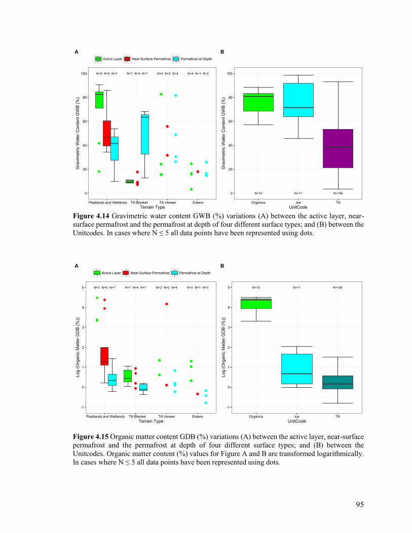
95
Figure 4.14 Gravimetric water content GWB (%) variations (A) between the active layer, near-
surface permafrost and the permafrost at depth of four different surface types; and (B) between the
Unitcodes. In cases where N ≤ 5 all data points have been represented using dots.
Figure 4.15 Organic matter content GDB (%) variations (A) between the active layer, near-surface
permafrost and the permafrost at depth of four different surface types; and (B) between the
Unitcodes. Organic matter content (%) values for Figure A and B are transformed logarithmically.
In cases where N ≤ 5 all data points have been represented using dots.
N=8 N=8 N=7 N=7 N=4 N=7 N=4 N=2 N=4 N=4 N=1 N=3
0
20
40
60
80
100
Peatlands and Wetlands Till Blanket Till Veneer Eskers
Terrain Type
Gra
vim
etr
ic W
ate
r C
on
ten
t G
WB
(%
)
Active Layer Near-Surface Permafrost Permafrost at Depth
A
N=15 N=11 N=1560
20
40
60
80
100
Organics Ice Till
UnitCode
Gra
vim
etr
ic W
ate
r C
on
ten
t G
WB
(%
)
B
N=3 N=8 N=7 N=7 N=4 N=7 N=2 N=2 N=4 N=3 N=1 N=3
-1
0
1
2
3
4
5
Peatlands and Wetlands Till Blanket Till Veneer Eskers
Terrain Type
Log
(O
rga
nic
Matt
er
GD
B (
%))
Active Layer Near-Surface Permafrost Permafrost at Depth
A
N=15 N=11 N=156
-1
0
1
2
3
4
5
Organics Ice Till
UnitCode
Log
(O
rga
nic
Matt
er
GD
B (
%))
B

96
with the median of nearly 65%.
Water content GWB was also compared between the Unitcodes (classification of
sample types based on the information from the drill logs, Figure 4.14B). Water contents
were found to be very high in “organic” and “ice” logged samples with medians of 81%
and 72%, but comparatively low in “till” samples with the median of about 39%. The high
water content GWB in the active layer of peatlands and wetlands, but low in till blanket
and till veneer terrains is well explained by the organic nature of core samples from the
former terrain.
4.3.4.2. Organic Matter Content GDB (%) Variations
In peatlands and wetlands, organic matter content was very high in the active layer,
followed by the near-surface permafrost and was comparatively low at depth in permafrost
(Figure 4.15). Organic matter content of the active layer and near-surface permafrost were
comparable in till blanket terrain, but varied more than threefold in the eskers. In till veneer,
the near-surface permafrost was characterized with very high organic matter content, but
was comparatively low in the active layer and especially at depth in permafrost. In
summary, organic matter content was high in peatlands and wetlands and till veneer
terrains, but was very low in till blanket and esker terrains.
Organic matter content between sample types was observed to be very high in
samples logged as “organics” with median of about 80%. Similarly, ice-rich samples were
also observed to contain organic materials, however much less than the organic samples.
Till samples contained the lowest organic matter contents between 0 and 1% (Figure
4.15B). As most samples from permafrost at depth were logged as “till”, and from Figure
4.15A it is clear that deep till or till with ice-rich materials at depth contains less organic

97
carbon. In summary, organic matter content varied with depth for most terrains, and was
very high in the active layer and in the near-surface permafrost at peatlands and wetlands
terrain.
4.3.4.3. Variations in Total Soluble Cation Concentration
Soluble cation concentration in the near-surface permafrost was higher and more
than double than that in the overlying active layer at the majority of sites from till blanket,
and in few sites from peatlands and wetlands, till veneer and esker terrains (Figure 4.16A
and B). Conversely, the majority of sites from peatlands and wetlands terrain contained
higher soluble cation concentrations in the active layer than in the underlying permafrost.
In peatlands and wetlands terrain, the median soluble cation concentration at depth in
permafrost was higher than the median soluble cation in the near-surface permafrost. This
is due to increased concentration of soluble cations below the depth of lower boundary of
the near-surface permafrost at few sites (e.g. 2011 and 1009) (Figure 4.10c and f). In till
blanket terrain, soluble cation concentration between the near-surface permafrost and the
permafrost at depth were relatively similar, but in till veneer and eskers, soluble cations
in the near-surface permafrost was higher than those at depth in permafrost.
Enrichment ratios were determined for the respective sites using data presented in
Figure 4.16 by diving median total soluble cation concentration in the near-surface
permafrost by the median total soluble cation concentration in samples obtained from the
active layer. Permafrost enrichment ratios for specific sites ranged from less than 0.05 to
21, indicating several sites to be depleted or enriched in the active layer (Table 4.8, Figure
4.16A and B).

98
Figure 4.16 (A) Soluble cation concentration variations between the active layer, near-surface
permafrost and the permafrost at depth; and (B) median total soluble cation concentrations in
mineral soils of the active layer and in the top 1 m of underlying permafrost (N=15). In cases where
N ≤ 5 all data points in Figure 4.16A have been represented using dots.
N=8 N=8 N=7 N=7 N=4 N=7 N=4 N=2 N=4 N=4 N=1 N=3
0.0
0.5
1.0
1.5
2.0
2.5
3.0
3.5
Peatlands and Wetlands Till Blanket Till Veneer Eskers
Terrain Type
To
tal S
olu
ble
Catio
ns (
me
q/1
00 g
dry
soil)
Active Layer Near-Surface Permafrost Permafrost at Depth
A
1:1
2:1
1:2
more in permafrost←m
ore
in a
ctiv
e la
ye
r
↓
0
1
2
3
0 1 2 3
Soluble cation concentrations in the active layer (meq/100 g)
So
luble
catio
n c
once
ntr
ation
s in p
erm
afr
ost (m
eq
/10
0 g
)
Terrain Type Eskers Peatlands and Wetland Till Blanket Till Veneer
B
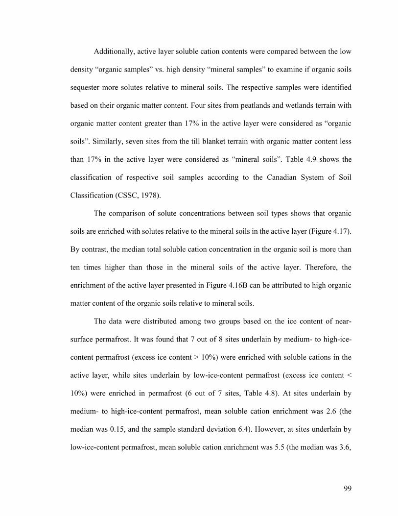
99
Additionally, active layer soluble cation contents were compared between the low
density “organic samples” vs. high density “mineral samples” to examine if organic soils
sequester more solutes relative to mineral soils. The respective samples were identified
based on their organic matter content. Four sites from peatlands and wetlands terrain with
organic matter content greater than 17% in the active layer were considered as “organic
soils”. Similarly, seven sites from the till blanket terrain with organic matter content less
than 17% in the active layer were considered as “mineral soils”. Table 4.9 shows the
classification of respective soil samples according to the Canadian System of Soil
Classification (CSSC, 1978).
The comparison of solute concentrations between soil types shows that organic
soils are enriched with solutes relative to the mineral soils in the active layer (Figure 4.17).
By contrast, the median total soluble cation concentration in the organic soil is more than
ten times higher than those in the mineral soils of the active layer. Therefore, the
enrichment of the active layer presented in Figure 4.16B can be attributed to high organic
matter content of the organic soils relative to mineral soils.
The data were distributed among two groups based on the ice content of near-
surface permafrost. It was found that 7 out of 8 sites underlain by medium- to high-ice-
content permafrost (excess ice content > 10%) were enriched with soluble cations in the
active layer, while sites underlain by low-ice-content permafrost (excess ice content <
10%) were enriched in permafrost (6 out of 7 sites, Table 4.8). At sites underlain by
medium- to high-ice-content permafrost, mean soluble cation enrichment was 2.6 (the
median was 0.15, and the sample standard deviation 6.4). However, at sites underlain by
low-ice-content permafrost, mean soluble cation enrichment was 5.5 (the median was 3.6,

100
Table 4.8 Enrichment ratio of soluble cation concentration of near-surface permafrost for
several sites in various terrains, near Lac de Gras, N.W.T
Median Total Soluble
Cation Concentration
(meq./100g dry soil)
Enrichment Ratio of
Near-Surface
Permafrost
Terrain-Type Borehole
ID Excess Ice Active Layer Permafrost
Peatlands and
Wetlands
1006 Low 0.60 2.50 4.2
1007 Medium To High 0.64 0.03 0.05
2011 Medium To High 3.04 0.11 0.04
2012 Medium To High 0.67 0.03 0.04
1009 Medium To High 2.10 0.26 0.12
1010 Medium To High 2.00 0.37 0.19
2015 Medium To High 0.12 0.10 0.83
1005 Low 0.66 1.34 2.0
Till Blanket
2004 Medium To High 0.22 0.18 0.81
1004 Low 0.08 0.31 3.9
2007 Low 0.09 0.29 3.2
2009 Low 0.05 0.18 3.6
Till Veneer 2018 Low 0.58 0.51 0.88
2013 Medium To High 0.07 1.29 18.4
Eskers 2028 Low 0.02 0.42 21

101
Table 4.9 Classification of soil types with respect to organic matter content of the active layer
according to the Canadian System of Soil Classification (CSSC, 1978).
Terrain-Type Borehole ID
Median Active-Layer
Organic Matter
Content (%)
Soil Type
Peatlands and
Wetlands
1005 >17 Organic
1006 89.4 Organic
1009 26.3 Organic
1010 27.4 Organic
Till Blanket
1004 1.31 Mineral
2004 2.81 Mineral
2005 1.57 Mineral
2006 1.33 Mineral
2007 1.98 Mineral
2033 2.85 Mineral
2009 1.03 Mineral

102
Figure 4.17 Active layer soluble cation contents compared between organic and mineral soils
Figure 4.18 Comparison of logarithm soluble cation enrichment ratios between the ice-rich and
ice-poor permafrost. A non-parametric (Mann-Whitney U) test showed the median enrichment
ratios between ice-rich and ice-poor sites to be significantly different (p-value = 0.009).
N=4 N=7
0.0
0.5
1.0
1.5
2.0
2.5
Organic Mineral
Active Layer Soil Types
To
tal S
olu
ble
Ca
tio
ns (
me
q/1
00
g d
ry s
oil)
N=8 N=7
-3
-2
-1
0
1
2
3
4
Ice-rich Ice-poor
Ice Content of Near-Surface Permafrost
Log
So
lub
le C
atio
n E
nrichm
ent
Ratio

103
and sample standard deviation 6.9, Figure 4.18). A non-parametric (Mann-Whitney U) test
showed that the median enrichment ratio between ice-rich and ice-poor sites was
significantly different (p-value = 0.009).
Variations in soluble cation concentration were also compared between the
Unitcodes (Figure 4.19). Soluble cations were much higher in samples logged as
“organics” followed by the “ice” and the “till” samples. In organic samples, the mean cation
concentration was 2.4 meq/ 100g dry soil (the median was 2.0, and the sample standard
deviation 1.8). In ice-rich samples, the mean cation concentration was 1.2 meq/100 g dry
soil (the median was 1.1, and the sample standard deviation 0.8). In till samples, the mean
was the lowest with 0.6 meq/100 g dry soil (the median was 0.4, and the sample standard
deviation 0.6).
4.3.5. Relation Between Electrical Conductivity and Total Soluble Cations
Electrical conductivity of water is a proxy for the concentration of dissolved ions
and is therefore expected to correlate with the total soluble cations present in a solution. In
this study, a large number of boreholes showed similar patterns between the electrical
conductivity and total soluble cations (see Appendix D). To test the relationship between
the two, the electrical conductivities in pore-water extracts were compared with the total
soluble cations determined in the laboratory (i.e. Ca2+, Mg2+, K+ and Na+). Figure 4.20
shows that the soil-water conductivity and total soluble cations were highly correlated
(R2=0.90, n=313).

104
Figure 4.19 Soluble cation concentration variations between the Unitcodes, for the cores obtained
near Lac de Gras, N.W.T.
Figure 4.20 The relation between electrical conductivity (Cpw) and total soluble cation
concentrations (Spw) (sum of soluble Ca2+, Mg2+, K+ and Na+) in pore-water extractions from the
active layer and permafrost samples, near Lac de Gras, N.W.T. The relation between two variables
is summarized by Spw = 8.83Cpw + 0.253 (R2 = 0.90, N = 313).
N=15 N=11 N=156
0.0
0.5
1.0
1.5
2.0
2.5
3.0
3.5
Organics Ice Till
UnitCode
Tota
l S
olu
ble
Cation
s (
me
q/1
00 g
dry
so
il)
0
10
20
30
40
50
60
70
0 2 4 6 8
Soil-Water Conductivity (mS/cm)
To
tal S
olu
ble
Cation
s (
me
q/l)

105
4.3.6. Relation Between Water Content GWB and Total Soluble Cations
Gravimetric water content GWB and soluble cation concentrations were compared
with each other to see if any relation existed between these two variables. Figure 4.21
shows the regression analysis between water content GWB and soluble cations (A) with
the data for the entire cores from every terrain; (B) with the data obtained from the active
layer; and (C) with the data obtained from the near-surface permafrost near Lac de Gras,
N.W.T. Regression analysis between water and cations yielded R2 values of 0.39, 0.51 and
0.53, respectively, and p-values < 0.05 (Figure 4.21) for the entire cores, in the active
layer as well as in the near-surface permafrost. However, further examination of the linear
fit between the two variables suggests that the residuals were not normally distributed. As
such, the significance of this relationship could be tested statistically despite the low p-
value. Nonetheless, an increased R2 in the active layer and especially in the near-surface
permafrost with most data from peatlands and wetlands indicates that some relationship
exists between water and soluble cations (Figure 4.21B and C).
4.3.7. Relation Between Organic Matter Content and Total Soluble Cations
A comparison of organic matter content and total soluble cation concentration
yielded an R2 value of 0.37 and a p-value < 0.05 (Figure 4.22A). However, further
examination of the linear fit between the two variables indicated that residuals were heavy
tailed, and hence non-normal. As such, the significance of this relationship could not be
built from the statistical analysis, despite the low p-value. The two variables were also
compared with data from the active layer and near-surface permafrost, however revealed
similar results as in the previous analysis (Figure 4.22C and 4.22D).

106
Figure 4.21 The relation between gravimetric water content GWB (%) and total soluble cations
meq/ 100g dry soil (A) for the entire depths, i.e., in the active layer, near-surface permafrost and at
depth in permafrost; (B) in the active layer; and (C) in the near-surface permafrost for the cores
obtained from various terrain in near Lac de Gras, N.W.T.
y = 0.02x - 0.183
R2 = 0.39
p-value = 0.000
0
2
4
6
8
0 20 40 60 80 100
Gravimetric Water Content GWB (%)
To
tal S
olu
ble
Ca
tion
s (
me
q/1
00
g d
ry s
oil) Terrain Type
Eskers
Peatlands and Wetlands
Till Blanket
Till Veneer
Across Entire DepthsAy = 0.03x - 0.231
R2 = 0.51
p-value = 0.000
0
2
4
6
8
0 20 40 60 80 100
To
tal S
olu
ble
Ca
tion
s (
me
q/1
00
g d
ry s
oil)
Terrain Type
Eskers
Peatlands and Wetlands
Till Blanket
Till Veneer
Active LayerB
y = 0.03x - 0.660
R2 = 0.53
p-value = 0.000
0
2
4
6
8
0 20 40 60 80 100
Gravimetric Water Content GWB (%)
To
tal S
olu
ble
Ca
tion
s (
me
q/1
00
g d
ry s
oil)
Terrain Type
Near-Surface PermafrostC
Eskers
Peatlands and Wetlands
Till Blanket
Till Veneer

107
A further examination of the relationship between the organic matter content and
total soluble cations based on the UnitCodes is presented in Figure 4.22B. Figure 4.22B
suggests that other than “organic” samples there is no evidence to believe that any
relationship exists between organic matter and soluble cations in gravel/cobbles, ice, sand,
silt, soil and till samples. This is supported by an increased r-squared value, i.e., R2 = 0.84
and 0.53 in the active layer and near-surface permafrost, respectively with most organic
data from the peatlands and wetlands terrain (Figure 4.22D), and a decreased R2 value 0.15
with few organic samples at depth in permafrost (Figure 4.22E).

108
Figure 4.22 The relation between organic matter content (%) and total soluble cations meq/ 100g
dry soil (A) with respect to terrain types for the entire cores in the active layer, near-surface
permafrost and at depth in permafrost; (B) with respect to UnitCodes; (C) in the active layer; (D)
in near-surface permafrost; and (E) in permafrost at depth for the cores obtained near Lac de Gras,
N.W.T.
y = 15.80x - 0.934
R2 = 0.37
p-value = 0.000
0
1
2
3
4
0 20 40 60 80 100
Organic Matter Content GDB (%)
To
tal S
olu
ble
Ca
tion
s (
me
q/1
00
g d
ry s
oil)
Terrain Type
Eskers
Peatlands and Wetlands
Till Blanket
Till Veneer
Across Entire Depths With Respect To Terrain TypesA
0
1
2
3
4
0 20 40 60 80 100
Organic Matter Content GDB (%)
To
tal S
olu
ble
Ca
tion
s (
me
q/1
00
g d
ry s
oil)
UnitCodes
Gravel/Cobbles
Ice
Organics
Sand
Silt
Soil
Till
Across Entire Depths With Respect To UnitCodesB
y = 0.03x + 0.038
R2 = 0.84
p-value = 0.000
0
1
2
3
4
0 20 40 60 80 100
Organic Matter Content GDB (%)
To
tal S
olu
ble
Ca
tion
s (
me
q/1
00
g d
ry s
oil)
Terrain Type
Eskers
Peatlands and Wetlands
Till Blanket
Till Veneer
Active LayerC
y = 0.02x + 0.255
R2 = 0.53
p-value = 0.000
0
1
2
3
4
0 20 40 60 80 100
Organic Matter Content GDB (%)
To
tal S
olu
ble
Ca
tion
s (
me
q/1
00
g d
ry s
oil)
Terrain Type
Near-Surface PermafrostD
Eskers
Peatlands and Wetlands
Till Blanket
Till Veneer
y = 0.02x + 0.413
R2 = 0.15
p-value = 0.000
0
1
2
3
4
0 20 40 60 80 100
Organic Matter Content GDB (%)
To
tal S
olu
ble
Ca
tio
ns (
me
q/1
00
g d
ry s
oil)
Terrain Type
Eskers
Peatlands and Swamps
Till Blanket
Till Veneer
Permafrost At Depth

109
CHAPTER 5. DISCUSSION
5.1. Overview
In Chapter 4, the vertical and spatial distribution of water content GWB, organic
matter content and total soluble cations were examined between depths, and also between
terrain types. Geochemical distinctions between the active layer, near-surface permafrost
and the permafrost at depth were evident at sites in each terrain type. Differences were also
observed between terrain types, and this was mainly attributed to type of sediment. This
chapter discusses the observed profiles and patterns in more detail. First, in order to support
the results of total soluble cations and provide rationale to the near-surface ionic
enrichment of permafrost in this study, the results from three distinct water extraction
techniques (Section 3.4.1) are discussed. The second section examines the relation between
soil texture and water content GWB, to assess the relative importance of soil type on water
and ground ice content variability. The third section discusses the factors associated with
variation in water, organic matter and soluble cations between the active layer, near-surface
permafrost and the permafrost at depth, and also between terrain types. This section also
compares geochemical profiles of this study with previous studies from differing
environments. The last section discusses the observed patterns of water, organic matter and
soluble cations to infer the depth of thaw unconformity at one of the sites from till veneer
terrain.

110
5.2. Effect of Soil-Water Extraction Method on the Concentration of Soluble
Cations
This study used the pore water extraction technique, i.e., Method 1 and Method 3,
to measure the concentration of soluble cations present in soil-water (e.g. Kokelj et al.,
2002; Kokelj and Burn, 2003). Although most studies in permafrost geochemistry use the
same method, some studies have also considered the leachate method, i.e., Method 2, in
which permafrost samples are thawed and dried, and a pre-determined soil:water ratio,
(extraction ratio) ranging from 1:1 to 1:25 by mass is used to extract the leachate water
(e.g. Blum et al., 2002; Keller et al., 2007). Fontaine (2016) compared these two water
extraction techniques and suggested that the use of Method 3 underestimates the
concentration of total soluble cations by 2 to more than 20 times relative to Method 2.
Based on this study, the enrichment of soluble cations in the near-surface permafrost in
studies from Kokelj et al. (2002) and Kokelj and Burn (2005) could have been biased as a
result of using pore water extraction method.
The results obtained from soil-water sampling using Method 2 and Method 3 in this
study however contradicts the aforementioned observation (Section 3.4.1). The
concentration of soluble cations i.e. Ca2+, Mg2+, K+ and Na+ is much higher in pore water
extracts obtained from Method 3, while those obtained from Method 2 are lower. A plot
showing the relative difference of Method 3 with Method 2 is presented in Figure 5.1. The
figure shows the concentration of Ca2+ and Mg2+ ions to vary the most, while K+ and Na+
ions have smaller differences. Because a predetermined extraction ratio (1:1) was
employed for both methods, while sufficient time was also given to undergo dissolution,
the low concentration of soluble cations from Method 2 indicates possible effects of drying

111
Figure 5.1 Relative difference of soluble cations obtained from Method 3 and Method 2. The
relative difference is defined by subtracting the concentration of soluble cations obtained from
Method 2 from the concentration of Method 3.
-0.25
0.00
0.25
0.50
0.75
1.00
162-5 162-6 163-4 165-17
SampleID
Rela
tive
Diffe
rence
Calcium
Magnesium
Potassium
Sodium
Relative Difference of Method 3 with Method 2

112
on samples which subdues the high ion contents present in soil water. In addition, an
extraction ratio greater than 1:1 allows an increase in the amount of soluble cations in the
leachate water, because of higher dissolution rates. Thus, the high values of leachate
conductivity in studies from Fontaine (2016) was likely simply a result of using a higher
extraction ratio (1:10). Therefore, the results of the pore water geochemistry and the related
near-surface ion enrichment of permafrost in studies from Kokelj et al. (2002) and Kokelj
and Burn (2005) are likely not biased based on data presented here.
5.3. Relation Between Gravimetric Water Content GWB and Soil Texture
In order to assess the relative importance of soil type for water and ground ice
content variability, the relation between water content GWB and soil texture was
examined. Since, water and ground ice content in permafrost are closely related to soil
porosity and pore geometry, finer-textured soils (e.g. “frost-suceptible” silts) are known to
draw water towards a freezing front (French, 2007), leading to the development of
segreated ice. In this study, the results of grain size analysis suggested higher silt contents
in peatlands and wetlands and till veneer terrains in comparison to other terrains (Appendix
E), thus indicating high potential for ground ice development in the former two terrain
types. The depth profiles of gravimetric water content GWB presented in Section 4.3.1 and
the comparison of water content GWB between terrain types (Figure 4.14) shows high
water content GWB in peatlands and wetlands and till veneer terrains relative to till blanket
and esker terrains. Thus, soil type represents a major influence on water and ground ice
content variability in this study area. However, it is also important to note the influence of
organic contents at a few sites from peatlands and wetlands terrain. For example, sites

113
characterized by very high organic matter content in the active layer and near-surface
permafrost (1005, 1006 and 1010) have high water content GWB, but no excess ice
contents (Figure 4.2). This is because organic soils have lower bulk density and high
porosity compared with mineral soils. Thus, as Morse et al. (2009) suggest, it is important
to handle gravimetric water content data carefully because high moisture content may be
indicative of high organic matter content rather than high ice content.
In order to examine if a significant relationship exists between the water content
GWB and soil texture in data obtained from various sites, a regression analysis was
conducted. Figure 5.2 shows statistically significant results (p-values = < 0.05) between
water content GWB vs. clay content (%), silt content (%) and sand content (%) in
permafrost samples with r-squared values of (0.15, 0.15 and 0.16, respectively). Water
content GWB increased in fine-grained sediments (%) (i.e. clay and silt), while it decreased
in the coarser sediments (i.e. sand). These results support the observed high water content
GWB values in the near-surface permafrost and in permafrost at depth for the peatlands
and wetlands and till veneer terrains as till samples in those terrain types consisted of more
fine-grained sediments than in till blanket or the esker terrains (Figure 5.2 A, B and C). In
contrast, decreasing water content GWB was evident in the coarser sediments. However,
points from the esker as well as till blanket sites which were expected to exemplify this
relation are not too close to the line of best fit. Although the regression provides with
some expected results, there is a significant amount of scatter in the plots indicating that
other factors also influence these relations. One such factor may be the varying soil
properties, such as bulk density, in samples from different terrain types.

114
Figure 5.2 Comparison of water content GWB with Clay Content (%), Silt Content (%) and Sand
Content (%) in samples obtained from various terrain types from Lac de Gras, N.W.T
y = 3.7x + 24.724
R2 = 0.15
p-value = 0.002
A
0
25
50
75
100
0 2 4 6 8 10
Clay Content (%)
Wate
r C
onte
nt
GW
B (
%)
y = 0.44x + 22.506
R2 = 0.15
p-value = 0.001
B
0
25
50
75
100
0 25 50 75 100
Silt Content (%)
y = - 0.40x + 62.643
R2 = 0.16
p-value = 0.001
C
0
25
50
75
100
0 25 50 75 100
Sand Content (%)

115
The results of the water content GWB and soil texture obtained here is quite
comparable with the results from the western Arctic. For example, Kokelj and Burn (2005)
documented an inverse association of sand content and the ice content of near-surface
permafrost at a site in sandy silt alluvium, although in clayey silt alluvium excess ice
contents increased due to high silt contents. Similarly, Morse et al. (2009) found that ice-
rich permafrost in the outer Mackenzie Delta was associated with soils normally composed
of at least 40% silt. In the Illisarvik drained lake basin, Mackay and Burn (2002) found
aggradation ice development in frost-susceptible organic rich silts, while was very little in
areas with sandy soils.
5.4. Vertical and Spatial Distribution: Gravimetric Water Content GWB, Organic
Matter Content and Total Soluble Cations
5.4.1. Gravimetric Water Content GWB (%)
The vertical and spatial distribution of water and excess ice contents from four
terrain types indicated that near-surface permafrost at a majority of sites from peatlands
and wetlands and till veneer terrains contained high water content GWB and excess ice
(Figure 4.2 and 4.4). This zone of high excess ice content in the near-surface permafrost,
also termed “transient layer” by Shur et al. (2005), is documented in many studies from the
western Arctic (e.g. Kokelj et al., 2002; Kokelj and Burn, 2003; O' Neill and Burn, 2012).
This zone of ice enrichment can be attributed to the annual flux divergence between the
downward moisture migration from the active layer into frozen ground and upward out of
permafrost, seasonally in summer and winter, respectively (Cheng, 1983). Mackay (1972)
further introduced the term aggradational ice for the ice-rich zone, and emphasized that

116
ice-lenses present at the base of the active layer may be trapped by an aggrading permafrost
table due to climate cooling, vegetation change or sedimentation.
Cheng’s (1983) hypothesis on segregated ice development is quite relevant for sites
from peatlands and wetlands terrain. In peatlands and wetlands terrain, high ice content in
the near-surface permafrost was often associated with frost-susceptible silts indicating high
potential for segregated ice development (Appendix E). Photos of cores showing ice lenses
from the near-surface permafrost of two different sites are given in Figure 5.3. Similarly,
Mackay’s (1972) hypothesis on near-surface aggradational ice is applicable at sites from
the till veneer terrains. At this terrain, site (2018 and 2013) from Hill 2 and Valley groups,
respectively were located either in low-lying depression or just at the bottom of the hill
where permafrost aggradation likely coincided with sedimentation, which resulted in the
development of near-surface ice-rich zone (Figure 3.5 and 4.4). In addition, the results of
the grain size analysis also suggest high silt contents for this particular terrain, indicating
high potential for ground ice development (Appendix E).
The active layer water content GWB at sites from peatlands and wetlands terrain
was significantly higher (see Table 4.8) than in sites of any other terrains (Figure 4.14).
This is due to the presence of high organic matter content in the uppermost layer of those
terrains (Figure 4.15), which contain lower bulk density in comparison to the mineral soils.
The comparison of water content GWB between the Unitcodes in Figure 4.14B also supports
this assumption as water content GWB tended to be high in organic samples, with the
median of about 80%. However, other factors also need consideration. For example,
conditions might have been favored by the lower relief at peatland and wetland sites, due
to poor drainage or drainage convergence resulting in high moisture availability in the

117
Figure 5.3 Core photos showing ice lenses present in the near-surface permafrost at two
different sites from peatlands and wetlands terrain near Lac de Gras, N.W.T.

118
active layer. By contrast, water content GWB of the active layer in till blanket and esker
terrains were comparatively low, which is explained by the coarser grain size as well as the
low organic matter content of the active layer in these terrains. Fontaine (2016) reported
similar results from the western Canadian Arctic where a positive association between
water and organic matter content described the uppermost 2 m of a sedge meadow site
corresponding to an organic rich zone, whereas in sites from thaw slumps (characterized
by low organic contents), gravimetric water content GWB was the lowest in the active
layer (< 60% GDB). Several distinctions in the active layer water content GWB should be
noted, especially from peatlands and wetlands, till veneer and esker terrains. Water content
GWB of the active layer at sites from these terrains were quite variable for the data obtained
between two exterior pits, or between pits and borehole. This variation corresponds to the
small-scale variability at sites existing due to subtle differences in relief, drainage, soils
and vegetation conditions over distances of 1–15 m.
In peatlands and wetlands and till veneer terrains, water content GWB of permafrost
normally declined with depth, but a few sites in those terrains were associated with
extremely high water and excess ice contents of up to 98% and 75%, respectively at depth
(Figure 4.2c, 4.2e, 4.2f, 4.2g and 4.4a). This is due to the high ice-segregation at the bottom
of the profiles, which were often associated with frost-susceptible tills of high silt contents.
The depth profiles of water content GWB from Section 4.3.1 as well as the comparison of
water content GWB between Unitcodes supports this argument as “till” samples contain
water content GWB up to 95%. The results of water content GWB and excess ice content
presented here contrasts with previous studies from the western Arctic. For example, the
deeper zones of increased moisture contents from Herschel Island are reported to be only

119
20 to 30 cm thick with ice lenses of about 2 cm (Kokelj et al., 2002), but in the present
study the zones of increased water content GWB at depth consisted between 50 to 100 cm,
and ice lenses at least 10 cm thick. Similarly, the deepest zones of ice accumulation on
hummocky tops of Inuvik are reported to contain only 12% excess-ice (Kokelj and Burn,
2003), whereas in this study, the average volumetric ice content in hummocky areas from
the Valley group are reported to contain more than 50% excess-ice.
5.4.1.1. Gravimetric Water Content GWB of the Hillslopes
The observed distinctions in the water content GWB profiles of the hillslopes
(especially from Hill 1 and Hill 3), depending upon the local positions of boreholes,
indicate the influence of erosive as well as accumulative nature of the slope materials that
are common at hill slope and hill bottom, respectively. For example, sites from Hill 1 and
Hill 3 groups, in till blanket terrain show excess ice content much closer to the ground
surface at the top of the hill, but as it approaches the slope and the hill bottom excess ice
content is either absent at the same depth interval, or gets much deeper into the ground
surface (Figure 4.3b, c, d, e and g). Core photos showing high excess ice contents in
permafrost at depth from various sites in till blanket terrain are provided in Figure 5.4.
Previous studies in western Arctic Canada have provided important evidence on buried
glacial ice near the northwest limit of the Laurentide Ice Sheet (Mathews and Mackay,
1960; Mackay et al., 1972). In the western Arctic Canada, buried glacial ice from the
Laurentide Ice sheet is supposed to have been preserved for more than 10 ka within large
moraine belts, hummocky till and glaciofluvial deposits (French and Harry, 1990). Given
the long glacial history of this area

120
Figure 5.4 Core photos showing high excess ice contents in permafrost at depth for the till blanket
terrain near Lac de Gras, N.W.T.

121
attributed to the Late Wisconsinan Laurentide ice sheet, which retreated from the region
approximately 9000 years ago (Kerr et al., 1997), it is possible that glacial thrusting and
shearing emplaced unconsolidated frozen sediments into the ice, which in the present
context is still buried underneath ablation till.
5.4.2. Organic Matter Content GDB (%)
The active layer and near-surface permafrost from most sites contained high
amounts of organic matter, while the permafrost at depth contained very little (Figure 4.15).
Organic matter content was highly variable between terrain types, however a general
similarity in profiles was observed in peatlands and wetlands, till blanket and eskers. In
these terrain types, organic matter content usually declined with depth and was the lowest
at depth in permafrost (Figure 4.15). By contrast, till veneer was observed with very high
organic matter content in the near-surface permafrost, while in the active layer and at depth
it was relatively low.
Organic matter content was highest in the active layer of peatlands and wetlands,
with values of up to 90% (Table 4.6). This is due to the presence of thick layers of peat (up
to 2.5 m thickness) near the surface (Figure 4.6). Similarly, active layers in other terrain
types also contained organic matter, but the values were very low, less than 5%. This is
likely due to surface conditions as well as a harsher growing environment in unconsolidated
tills which incorporate very little organic materials in the active layer. Similarly, the near-
surface permafrost also had some of the highest organic matter contents. This was mostly
the case in peatlands and wetlands and till veneer terrains, but in other terrains were very
low, less than 3% (Table 4.6). In peatlands and wetlands, the thick layers of peat explain

122
the high concentration of organic matter in the near-surface permafrost (Figure 4.6). Other
possible mechanisms include cryoturbation (Dredge et al., 1994), and the burial of surface
organic matter followed by permafrost aggradation which transfers organic matter content
into the deeper horizons (e.g. Kokelj et al., 2009). The latter mechanism is relevant at sites
from till veneer terrain because the majority of them were located in low-lying depressions
or just at the bottom of the hills where permafrost aggradation likely coincided with
sedimentation. Organic matter content was the lowest at depth in permafrost for all terrain
types investigated. The absolute concentration of carbon in deeper unconsolidated
Quaternary deposits had a range of 0.40–4.00% of dry weight.
5.4.3. Total Soluble Cations (meq/100 g dry soil)
Most studies from the western Arctic report distinct geochemical characteristics
between the active layer and underlying permafrost, based on the increased concentrations
of soluble cations in the near-surface permafrost (e.g. Kokelj and Lewkowicz, 1999; Kokelj
et al., 2002; Kokelj and Burn, 2003; Kokelj and Burn, 2005). In this study, the near-surface
permafrost in mineral soils is enriched with soluble cations similar to observations from
other regions. For example, the median soluble cation concentration at the till steep slope
and hill bottom sites (1004, 2007, 2009 and 2013) from till blanket and till veneer terrains,
and at the esker site (2028) is higher in near-surface permafrost than the overlying active
layer (Table 4.8 and Figure 4.16B). However, in this study, the result of soluble cations
obtained from organic soils, contrasts with those obtained from mineral soils. In organic
soils, the active layer soluble cation concentration is much higher than the underlying
mineral soil permafrost. For example, the median soluble cation concentration of the active

123
layer obtained from six peatland and wetland sites (1007, 2011, 2012, 1009, 1010 and
2015) is much higher in the organic active layer than the underlying mineral soil permafrost
(Table 4.8 and Figure 4.16B). Further, the comparison of active layer soluble cations
between organic soils and mineral soils revealed that organic soils contain more solutes
than mineral soils (Figure 4.17). These results suggest that in the Lac de Gras area, organic
soils are enriched with solutes relative to tills and glaciofluvial deposits, and since the
organics are primarily at the surface or within the active layer, the active layer is therefore
solute rich with respect to underlying mineral soil permafrost.
A recent study conducted by Fontaine (2016) near the Mackenzie delta region
found similar enrichment in the active layer. Three out of her 8 sites, associated with high
organic matter content, contained significantly higher concentration of soluble cations in
the active layer than the underlying permafrost. The active layer enrichment of this study
is quite comparable with Fontaine (2016), because the enriched sites in peatlands and
wetlands terrain were highly organic in nature. In addition, the comparison of solute
concentration between sample types also supports this result as organic samples show
highest concentrations of soluble cations (Figure 4.19). Few enrichments in the active layer
are also reported from the disturbed sites, at Herschel Island, but the sites had little or no
vegetation (Kokelj et al., 2002).
The near-surface cation enrichment of sites observed in this study is related to the
geomorphic setting of each terrain type, and may be explained with processes that are
documented in previous studies. In peatlands and wetlands terrain, high concentration of
soluble cations in the near-surface permafrost at the peatland sites (1005 and 1006) is
explained by high organic matter content, which extended up to 2.5 m depth in permafrost

124
(Figure 4.16B and Figure 4.10). The high concentration of soluble cation in the uppermost
surface of low-lying site 2018 can be attributed to high volume of organics present in
the active layer.
In profiles, zones of increased cation concentrations corresponded with ice-rich
intervals at depth in permafrost, indicating that soluble materials may be drawn with water
along thermal gradients (Cary and Mayland 1972; Qui et al., 1988; Chuvilin et al., 1998;
Brouchkov 2000). This was especially true for sites in peatlands and wetlands and till
veneer terrains (Figure 4.10 and 4.12), as samples in these terrains consisted of high silt
contents, so solute accumulation may have accompanied segregated ice development.
The absolute concentration of soluble cations obtained in this study is very low
compared to previous studies from northwestern Canada. Other than the organic samples,
where the mean total soluble cation concentrations reach up to 3.43 meq/100 g dry soil in
the active layer, and 1.48 meq/100 g dry soil in permafrost (Table 4.1), due to their lower
bulk density, mineral soils constitute very low soluble cation concentration in the active
layer and underlying permafrost (Table 4.2). In mineral soils, the mean total soluble cation
concentration of the active layer from various sites in till blanket terrain is often less than
0.50 meq/100 g dry soil, and in permafrost, less than 0.40 meq/100 g dry soil (Table 4.2).
Previous studies from the Mackenzie Delta and Herschel Island report higher concentration
of soluble cations from the active layer and permafrost of various terrain types (Table 5.1).
In Mackenzie Delta, a range of forest-terrain types contained soluble cations up to three-
fold higher in the active layer, and five times higher in permafrost, than those observed in
mineral soils of this study (Table 5.1). Even when active layers and permafrost soluble
cation concentrations are compared with undisturbed terrain types of Herschel Island, the

125
Table 5.1 Concentration of soluble cations reported from the mineral soils of active layer
and permafrost from previous studies in northwestern Canada.
Mackenzie Delta
(Kokelj and Burn, 2005)
Herschel Island
(Kokelj et al., 2002)
Lac de Gras Area
(This Study)
Terrain
Type
Total Soluble
Cations (meq/100 g
dry soil)
Terrain
Type
Total Soluble
Cations (meq/100 g
dry soil)
Terrain
Type
Total Soluble
Cations (meq/100 g
dry soil)
Active
Layer
Permafrost Active
Layer
Permafrost Active
Layer
Permafrost
Point-Bar
Willow 2.06 3.83
Undisturbed
Plateau
0.25–
1.5 12–14
Till
Blanket
0.08–
0.94
0.04–0.50
Point-Bar
Alder 1.54 2.15
Undisturbed
Plateau
0.25–
6 8–14
Till
Veneer
0.17–
0.90
0.25–1.39
Spruce-
Alder-
Bearberry
0.64 2.09
Undisturbed
Stable
Slope
< 0.25 5
Eskers
0.02–
0.08
0.08–0.31
Spruce-
Feathermoss 0.49 1.24
Disturbed
AL
Detachment
Slides
2–10 12
Spruce-
Crowberry-
Lichen 0.38 1.62
Disturbed
AL
Detachment
Slides
2–12 12

126
absolute concentrations of soluble cations are very low in this study. This difference in
soluble cation concentrations from previous studies might be associated with materials of
different origins. Since, Lac de Gras area has a contrasting geomorphic and regional setting
from other areas in the north, this difference might be a major contributing factor to the
observed low concentration of soluble cations in mineral soils.

127
CHAPTER 6. CONCLUSIONS
This thesis examined the vertical and spatial patterns of water content GWB,
organic matter content (%) and total soluble cations (meq./100 g dry soil) near Lac de Gras,
N.W.T. The following conclusions can be drawn from this study.
1. In the Lac de Gras area, organic soils are enriched with solutes relative to tills and
glaciofluvial deposits, and since the organics are primarily at the surface or within
the active layer, the active layer is solute rich with respect to underlying permafrost.
2. Active layer and underlying permafrost are geochemically distinct, but unlike
previous studies from other areas, this difference is attributed to organic soils,
which sequester more solutes in the active layer, relative to underlying mineral soil
permafrost.
3. Near-surface solute enrichment of permafrost, similar to most previous studies
from northwestern Canada, is evident at some sites in each terrain type.
4. The concentration of soluble cations at depth in permafrost was generally low, but
the zones of increased cation concentrations at depth corresponded with ice-rich
intervals.
5. Organic matter content was highest in the active layer of peatlands and wetlands
terrain, and in other terrains the uppermost layers were characterized by relatively
low organic matter. Organic matter content also declined with depth, i.e., it was
highest in the active layer, followed by the near-surface permafrost and was lowest
at depth in permafrost for all terrain types.

128
6. In comparison with previous studies from northwestern Canada, the absolute
concentration of soluble cations in the active layer and near-surface permafrost of
mineral soils is about one order of magnitude lower in the Lac de Gras area.

129
BIBLIOGRAPHY
Andersson, J. G. (1906). Solifluction; a component of subaerial denudation. Journal of
Geology, 14, 91–112.
Anderson, D. M., and Morgenstern, N. R. (1973). Physics, chemistry, and mechanics of
frozen ground. A review. In Permafrost: The North American contribution to the 2nd
International Conference on Permafrost, Yakutsk, 13-28 July. pp. 257–288.
Associate Committee on Geotechnical Research (ACGR). (1988). Canadian glossary of
permafrost and related ground-ice terms, technical memorandum No. 142. National
Research Council of Canada: Ottawa, ON; 156 pp.
Bakhman, V.I., and Efemiov, A.L. (1962). Chemical composition of water and bottom
sediments in some thermokarst lakes of central Yakutia. Akad. Nauk SSSR Sibirskoe
otd – ie Inst Merzlotovedeniia Mnogoletnemerzlye, p. 114–122.
Beuselinck, L., Govers, G., Poesen, J., Degraer, G., and Froyen, L. (1998). Grain-size
analysis by laser diffractometry: comparison with the sieve-pipette method. Catena,
32(3-4), p. 193–208.
Blum J. D., Klaue A., Nezat C. A., Driscoll C. T., Johnson C. E., Siccama T. G., Eagar C.,
Fahey T. J., and Likens G. E. (2002). Mycorrhizal weathering of apatite as an
important calcium source in base-poor forest ecosystems. Nature 417:729–731.
Bockheim J. G., Everett L. R., Hinkel K. M., Nelson F. E., and Brown J. (1999). Soil
organic carbon storage and distribution in arctic tundra, Barrow, Alaska. Soil Science
Society of America Journal 63: 934–940.
Bockheim, J. G. (2007). Importance of cryoturbation in redistributing organic carbon in
permafrost-affected soils. Soil Science Society of America Journal, 71, 1335.
Bouchard M. (1974). Geologie de depots de L’Ile Herschel, Territoire du Yukon. (Thèse
M.Sc. non publié). University de Montreal, Montreal, Canada.
Brouchkov, A. (2000). Salt and water transfer in frozen soils induced by gradients of
temperature and salt content. Permafrost and Periglacial Processes, 11: 42–49.
Brown, R.J.E. (1967). Permafrost in Canada. Geological Survey of Canada Map 1246a.
National Research Council of Canada, Ottawa, Ontario.
Brown, J., Gray, S., and Webster, W. (1967). Chemical and related properties of permafrost
section from Fairbanks, Alaska. USA. CRREL Technical Note, 18 p.

130
Brown, J. (1969). Ionic concentration gradients in permafrost, Barrow, Alaska. Cold
Regions Research and Engineering Lab Hanover NH (No. CRREL-RR-272).
Burn C.R. (1997). Cryostratigraphy, paleogeography, and climate change during the Early
Holocene warm interval, western Arctic coast, Canada. Canadian Journal of Earth
Sciences, 34, 912–925.
Burn C. R. (2004). The thermal regime of cryosols. In Cryosols: Permafrost-affected Soils,
Kimble JM (ed.). Springer-Verlag: Berlin, Germany; 391–413.
Burn C. R., and Michel FA. (1988). Evidence for recent temperature-induced water
migration into permafrost from tritium content of ground ice near Mayo, Yukon
Territory, Canada. Canadian Journal of Earth Sciences 25: 909–915.
Burt T. P., and Williams P. J. (1976). Hydraulic conductivity in frozen soils. Earth Surface
Processes 1: 349–360.
Canada Soil Survey Committee. (1978). The Canadian system of soil classification.
Research Branch, Canada Department of Agriculture.
Canamera Gelogical (1996). Lytton Minerals Limited Jericho Diamond Project: Bulk
Sample Class A Land Use Application. Report submitted to Indian and Northern
Affaira Canada, p. 46.
Cary, J. W., and Mayland, H. F. (1972). Salt and water movement in unsaturated frozen
soil. Soil Science Society of America Journal, 36(4), p. 549–555.
Cheng, G. (1983). The mechanism of repeated-segregation for the formation of thick
layered ground ice. Cold Regions Science and Technology, 8(1), p. 57–66.
Chin, K. S., Lento, J., Culp, J. M., Lacelle, D., and Kokelj, S. V. (2016). Permafrost thaw
and intense thermokarst activity decreases abundance of stream benthic
macroinvertebrates. Global Change Biology, 22, p. 2715–2728.
Chizhov A. B., Chizhova N. I., Morkovina I. K., and Romanov VV. (1983). Tritium in
permafrost and ground ice. In Proceedings, 4th International Conference on
Permafrost, Fairbanks, Alaska, July 17–22, 1983, Vol. 1. National Academy Press:
Washington, DC; 1030–1035.
Chuvilin, E. M., Ershov, E. D., and Smirnova, O. G. (1998). Ionic migration in frozen soils
and ice. In Proceedings of the 7th International Permafrost Conference, Yellowknife,
N.W.T., 23–27 June 1998. Edited by A.G. Lewkowicz and M. Allard. Centre d’études

131
nordiques, Université Laval, Laval, Quebec. p. 167–171.
Diochon, A., Gregorich, E. G., and Tarnocai, C. (2013). Evaluating the quantity and
biodegradability of soil organic matter in some Canadian Turbic Cryosols. Geoderma,
202–203, 82–87.
Dredge, L.A., Ward, B.C., and Kerr, D.E. (1994). Glacial geology and implications for
drift prospecting in the Lac de Gras, Winter Lake, and Aylmer Lake map areas, central
Slave Province. In Current Research 1994-C; Geological Survey of Canada, p. 33–
38.
Dredge, L. A., Kerr, D. E., and Wolfe, S. A. (1999). Surficial materials and related ground
ice conditions, Slave Province, N.W.T., Canada. Canadian Journal of Earth Sciences,
36, p. 1227–1238.
Egginton, P. A., and French, H. M. (1985). Solifluction and related processes, eastern
Banks Island, N.W.T. Canadian Journal of Earth Sciences, 22(11), 1671–1678.
Environment Canada (2016). National climate data and information archive, climate
normals and averages, http://climate.weather.gc.ca/climate_normals/index_e.html.
[accessed February 2016].
Eshel, G., Levy, G. J., Mingelgrin, U., and Singer, M. J. (2004). Critical evaluation of the
use of laser diffraction for particle-size distribution analysis. Soil Science Society of
America Journal, 68(3), p. 736.
Fontaine, M. (2016). Ground ice content and geochemistry of active layer and permafrost
in northwestern Arctic Canada. (Master’s thesis). University of Ottawa, Ottawa,
Canada. Retrieved from www.ruor.uottawa.ca/handle/10393/33428.
French, H. M., and Harry, D. G. (1990). Observations on buried glacier ice and massive
segregated ice, western Arctic coast, Canada. Permafrost and Periglacial Processes,
1(1), 31–43.
French, H. M. (2007). The periglacial environment. 3rd edition. Longman, London, UK.
Frey K.E. and McClelland J.W. (2009). Impacts of permafrost degradation on arctic river
biogeochemistry. Hydrological Processes, 23(1), 169–182.
Gill, D. (1973). Ecological modifications caused by the removal of tree and shrub canopies
in the Mackenzie Delta. Arctic, 26: 95–111.
Guodong, C. (1983). The mechanism of repeated-segregation for the formation of thick

132
layered ground ice. Cold Regions Science and Technology, 8(1), 57–66.
Heginbottom, J.A., Dubreuil, M.A., and Harker, P.A. (1995). Canada-Permafrost. In
National Atlas of Canada 5th Edition, National Atlas Information Service, Natural
Resources Canada, Ottawa, Plate 2.1, MCR 4177.
Hinzman L.D., Deal C.J., McGuire A.D., Mernild S.H., Polyakov I.V. and Walsh J.E.
(2013). Trajectory of the Arctic as an integrated system. Ecological Applications, 23,
1837–1868.
Hugelius, G., Kuhry, P., Tarnocai, C., and Virtanen, T. (2010). Soil organic carbon pools
in a periglacial landscape: A case study from the central Canadian Arctic. Permafrost
and Periglacial Processes, 21(1), p. 16–29.
Hu, X., Holubec, I., Wonnacott, J., Lock, R., and Olive, R. (2003). Geomorphological,
geotechnical and geothermal conditions at Diavik Mines. In 8th International
Conference on Permafrost. Zurich, Switzerland. p. 18.
Huh, Y., Tsoi, M. Y., Zaitsev, A., and Edmond, J. M. (1998). The fluvial geochemistry of
the rivers of Eastern Siberia: I. Tributaries of the Lena River draining the sedimentary
platform of the Siberian Craton. Geochimica et Cosmochimica Acta, 62: 1657-1676.
Janzen, H.H. (1993). Soluble salts. In Soil sampling and methods of analysis. Lewis
Publishers, Boca Raton, Fla., p. 161–166.
Jorgenson M. T., Shur Y. L., and Pullman E. R. (2006). Abrupt increase in permafrost
degradation in Arctic Alaska. Geophysical Research Letters 33: L02503.
Kaiser, C., Meyer, H., Biasi, C., Rusalimova, O., Basukov, P., and Richter, A., (2007).
Conservation of soil organic matter through cryoturbation in arctic soils in Siberia.
Journal of Geophysical Research 112, G02017.
Karunaratne, K. C. (2011). A field examination of climate-permafrost relations in
continuous and discontinuous permafrost of the Slave geological province. (Doctoral
dissertation). Carleton University, Ottawa, Canada.
Keller, K., Blum, J. D., and Kling, G. W. (2007). Geochemistry of soils and streams on
surfaces of varying ages in Arctic Alaska. Arctic, Antarctic, and Alpine Research,
39(1), p. 84–98.
Kerr, D.E., Wolfe, S.A., and Dredge, L.A. (1997). Surficial geology of the Contwoyto Lake
map area (north half), District of Mackenzie, Northwest Territories. In Current

133
Research 1997-C, Geological Survey of Canada, p. 51–59.
Kjarsgaard, B.A. and Wyllie, R.J.S. (1994). Geology of the Paul Lake Area, Lac de Gras,
Lac de Sauvage Region of the Central Slave Province, District of Keewatin, N.W.T.
In Current Research. 1994-C, Geological Survey of Canada . 23– 32.
Kokelj, S. V., and Lewkowicz, A. G. (1999). Salinization of permafrost terrain due to
natural geomorphic disturbance, Fosheim Peninsula, Ellesmere Island. Arctic, 52(4),
p. 372–385.
Kokelj, S. V., Smith, C. A. S., and Burn, C. R. (2002). Physical and chemical
characteristics of the active layer and permafrost, Herschel Island, western Arctic
Coast, Canada. Permafrost and Periglacial Processes, 13(2), p. 171–185.
Kokelj, S. V., and Burn, C. R. (2003). Ground ice and soluble cations in near-surface
permafrost, Inuvik, Northwest Territories, Canada. Permafrost and Periglacial
Processes, 14(3), p. 275–289.
Kokelj, S. V., and Burn, C. R. (2005). Geochemistry of the active layer and near-surface
permafrost, Mackenzie delta region, Northwest Territories, Canada. Canadian
Journal of Earth Sciences, 42(1), p. 37–48.
Kokelj S. V., Lantz T. C., Kanigan J., Smith S. L., and Coutts R. (2009). Origin and
polycyclic behavior of tundra thaw slumps, Mackenzie Delta Region, Northwest
Territories, Canada. Permafrost and Periglacial Processes, 20, 173–184.
Kokelj S.V., and Jorgenson M.T. (2013). Advances in thermokarst research. Permafrost
and Periglacial Processes, 24(2), 108–119.
Kokelj, S. V., Lacelle, D., Lantz, T. C., Tunnicliffe, J., Malone, L., Clark, I. D. and Chin,
K.S. (2013). Thawing of massive ground ice in mega slumps drives increases in
stream sediment and solute flux across a range of watershed scales. Journal of
Geophysical Research: Earth Surface, 118, 681–692.
Konrad, J. M., and McCammon, A. W. (1990). Solute partitioning in freezing soils.
Canadian Geotechnical Journal, 27(6), 726–736.
Kling, G.W., O'Brien, J., Miller, M.C., and Hershey, A.E. (1992). The biogeochemistry
and zoogeography of lakes and rivers in arctic Alaska. Hydrobiologia, 240: 1-14.
Kopecký, M., and Čížková, Š. (2010). Using topographic wetness index in vegetation
ecology: does the algorithm matter. Applied Vegetation Science, 13(4), 450–459.

134
Kuhry, P., Grosse, G., Harden, J. W., Hugelius, G., Koven, C. D., Ping, C.-L.,
Schirrmeister, L., and Tarnocai, C. (2013). Characterisation of the Permafrost Carbon
Pool. Permafrost and Periglacial Processes, 24(2), p. 146–155.
Kudryavtsev, A., Dostovalov, B. N., and Garagulya, L. S. (1978). Radiation-heat balance
of the soil surface as a factor in the formation and dynamics of seasonally frozen soils
and permafrost. In Permafrost, Second International Conference, July 13–28, 1973:
USSR contribution. p. 18.
Lacelle, D., Juneau, V., Pellerin, A., Lauriol, B., and Clark, I.D. (2008). Weathering regime
and geochemical conditions in a polar desert environment, Haughton impact structure
region, Devon Island, Canada. Canadian Journal of Earth Sciences, 45, 1139–1157.
Lacelle, D., and Vasil’chuk, Y. K. (2013). Recent progress (2007-2012) in permafrost
isotope geochemistry. Permafrost and Periglacial Processes, 24(2), p. 138–145.
Lantz, T. C., Kokelj, S. V., Gergel, S. E., and Henry, G. H. (2009). Relative impacts of
disturbance and temperature: persistent changes in microenvironment and vegetation
in retrogressive thaw slumps. Global Change Biology, 15(7), p. 1664–1675.
Leibman, M. O., and Streletskaya, I. D. (1997). Land-slide induced changes in the chemical
composition of active layer soils and surface-water run-off, Yamal Peninsula, Russia.
In Proceedings of the International symposium on physics, chemistry, and ecology of
seasonally frozen soils, Fairbanks, Alaska, 10–12 June 1997. Edited by I.K. Iskandar,
E.A. Wright, J.K. Radke, B.S. Sharratt, P.H. Groenevelt, and L.D. Hinzman. CRREL
Special Report 97-10, Cold Regions Research and Engineering Laboratory (CRREL),
Hanover, N.H., p. 120–126.
Mackay, J. R. (1972). The world of underground ice. Annals of the Association of American
Geographers. 63, 1-22.
Mackay, J. R., Rampton, V. N., and Fyles, J. G. (1972). Relic Pleistocene permafrost,
western Arctic, Canada. Science, 176(4041), 1321–1323.
Mackay, J. R. (1980). The origin of hummocks, western Arctic coast, Canada. Canadian
Journal of Earth Sciences, 17, 996–1006.
Mackay, J. R. (1981). Active layer slope movement in a continuous permafrost
environment, Garry Island, Northwest Territories, Canada. Canadian Journal of
Earth Sciences, 18(11), 1666–1680.

135
Mackay, J. R. (1982). Active layer growth, Illisarvik experimental drained lake site,
Richards Island, Norwest Territories; in Current Research, Part A, Geological Survey
of Canada, Paper 82-1A, p. 123–126, 1982.
Mackay, J. R. (1983). Downward water movement into frozen ground, Western Arctic
coast, Canada. Canadian Journal of Earth Sciences, 20(1), p. 120–134.
Mackay, J. R. (1995). Active layer changes (1968 to 1993) following the forest-tundra fire
near Inuvik, N.W.T., Canada. Arctic and Alpine Research, 27(4), p. 323.
Mackay J. R., and Burn C. R., (2002). The first 20 years (1978-1979 to 1998-1999) of
active-layer development, Illisarvik experimental drained lake site, western Arctic
coast, Canada. Canadian Journal of Earth Sciences 39: 1657–1674.
Malone L., Lacelle D., Kokelj S.V. and Clark I.D. (2013). Impacts of hillslope thaw slumps
on the geochemistry of permafrost catchments (Stony Creek watershed, NWT,
Canada). Chemical Geology, 356, 38–49.
Mathews, W. H. and Mackay, J. R. (1960). Deformation of soils by glacier ice and the
influence of pore pressure and permafrost. Royal Society of Canada Transactions,
LIX, Series III, Section 4, 27–36.
McRoberts, E. C., and Morgenstern, N. R. (1974). The stability of thawing slopes.
Canadian Geotechnical Journal, 11(4), 447–469.
Mitchell, JK., Soga, K. (2005). Fundamentals of soil behaviour. John Wiley & Sons,
Hoboken, New Jersey.
Morse, P. D., Burn, C. R., and Kokelj, S. V. (2009). Near-surface ground-ice distribution,
Kendall Island Bird Sanctuary, Western Arctic coast, Canada. Permafrost and
Periglacial Processes, 20, 155–171.
National Wetlands Working Group. (1988). Wetlands of Canada. Ecological land
classification series, no. 24. Sustainable Development Branch, Environment Canada,
Ottawa, Ontario, and Polyscience Publications Inc., Montreal, Quebec, 452.
O'Donnell, J. A., Harden, J. W., McGuire, A. D., Kanevskiy, M. Z., Jorgenson, M. T., and
Xu, X. (2011). The effect of fire and permafrost interactions on soil carbon
accumulation in an upland black spruce ecosystem of interior Alaska: implications for
post‐thaw carbon loss. Global Change Biology, 17(3), 1461-1474.
O’Neill, H. B. and Burn, C.R. (2012). Physical and temporal factors controlling the

136
development of near-surface ground ice at Illisarvik, western Arctic coast, Canada.
Canadian Journal of Earth Sciences, 49, 1096–1110.
O'Sullivan, J. B. (1966). Geochemistry of permafrost, Barrow, Alaska. In Proceedings,
International Conference on Permafrost. National Academy of Sciences – National
Research Council Publication 1287. p. 30–37.
Osterkamp, T. E., and Burn, C. R., (2002), Permafrost, in Holton, J.R., Pyle, J., and Curry,
J.A., eds., Encyclopedia of Atmospheric Sciences: New York, Academic Press, p.
1717–1729.
Pewe, T. L., and Sellmann, P. V. (1973). Geochemistry of permafrost and Quaternary
stratigraphy. In Permafrost: North American Contribution to the Second International
Conference, Yakutsk, U.S.S.R. National Academy of Science Press, Washington,
D.C., pp. 166–170.
Phillips, M. R., Burn, C. R., Wolfe, S. A., Morse, P. D., Gaanderse, A. J., O'Neill, H. B.,
Shugar, D.H. and Gruber, S. (2015). Improving water content description of ice-rich
permafrost soils. In Proceedings of the GeoQuebec 2015 Conference, September 21–
23, Quebec, Canada. Canadian Geotechnical Society, Richmond, BC. 7 p.
Qui, G., Sheng, W., Huang, C., and Zheng, K. (1988). Direction of ion migration during
cooling and freezing processes. In Proceedings, Fifth International Conference on
Permafrost, 2-5 August, Trondheim, Norway. Trondheim, Norway: Tapir Publishers,
vol. 1, p. 442– 447.
Rampton V. N. (1988). Quaternary geology of the Tuktoyaktuk Coastlands, Northwest
Territories. Geological Survey of Canada Memoir 423.
Rempel, A. W. (2010). Frost heave. Journal of Glaciology, 56(200), 1122–1128.
Rydin, H., Jeglum, J. K., and Jeglum, J. K. (2013). The biology of peatlands, 2e. Oxford
university press.
Schirrmeister, L., C. Siegert, T. Kuznetsova, S. Kuzmina, A. Andreev, F. Kienast, H.
Meyer, and A. Bobrov (2002). Paleoenvironmental and paleoclimatic records from
permafrost deposits in the Arctic region of northern Siberia, Quat. Int., 89, 97–118
Schuur, E. A. G., et al. (2008), Vulnerability of permafrost carbon to climate change:
Implications for the global carbon cycle, BioScience, 58, 701–714.
Sheldrick BH. (ed.). (1984). Analytical methods manual 1984. Land Resource Research
137
Institute, Agriculture Canada, Ottawa, Canada, LRRI Contribution No. 84–30.
Shur, Y., Hinkel, K. M., and Nelson, F. E. (2005). The transient layer: implications for
geocryology and climate-change science. Permafrost and Periglacial Processes,
16(1), 5–17.
Stutter, M. I., and Billet, M. F. (2003). Biogeochemical controls on stream water and soil
solution chemistry in a High Arctic environment. Geoderma, 113: 127-146.
Smith, M. W. (1975). Microclimatic influences on ground temperatures and permafrost
distribution, Mackenzie Delta, Northwest Territories. Canadian Journal of Earth
Sciences, 12(8), p. 1421–1438.
Smith, MW. (1985). Observations of soil freezing and frost heave at Inuvik, Northwest
Territories, Canada. Canadian Journal of Earth Sciences, 22, 283–290.
Smith C. A. S.., Fox C. A., and Hargrave A. E. (1991). Development of soil structure in
some Turbic Cryosols in the Canadian low Arctic. Canadian Journal of Soil Science
71: 11–29.
Smith S. L., Romanovsky V. E., Lewkowicz A. G., Burn C. R., Allard M., Clow G. D.,
Yoshikawa K., and Throop J. (2010). Thermal state of permafrost in North America:
a contribution to the International Polar Year. Permafrost and Periglacial Processes
21: 117–135.
Tarnocai, C. (1999). The effect of climate warming on the carbon balance of Cryosols in
Canada. Permafrost and Periglacial Processes, 10(3), p. 251–263.
Tarnocai, C., Canadell, J. G., Schuur, E. A. G., Kuhry, P., Mazhitova, G., and Zimov, S.
(2009). Soil organic carbon pools in the northern circumpolar permafrost region.
Global Biogeochemical Cycles, 23(2).
Thienpont, J. R., Johnson, D., Nesbitt, H., Kokelj, S. V., Pisaric, M. F., and Smol, J. P.
(2012). Arctic coastal freshwater ecosystem responses to a major saltwater intrusion:
A landscape-scale palaeolimnological analysis. The Holocene, 22(12), p. 1451-1460.
Toner, J. D., Sletten, R. S., and Prentice, M. L. (2013). Soluble salt accumulations in Taylor
Valley, Antarctica: implications for paleolakes and Ross Sea Ice Sheet dynamics.
Journal of Geophysical Research: Earth Surface, 118(1), 198-215.
Washburn A.L. (1980). Geocryology: a survey of periglacial processes and environments.
John Wiley & Sons, New York, NY, 406 p.

138
Watanabe, K., Mizoguchi, M., (2002). Amount of unfrozen water in frozen porous media
saturated with solution. Cold Regions Science and Technology. 34, 103–110.
Wiken, E. B., Gauthier, D., Marshall, I., Lawton, K., and Hirvonen, H. (1996). A
perspective on Canada’s ecosystems. Canadian Council on Ecological Areas, 14.
Wilkinson, L., Harris, J., Kjarsgaard, B., Mcclenaghan, B., and Kerr, D. (2001). Influence
of till thickness and texture on till geochemistry in the Lac de Gras area, Northwest
Territories, with applications for regional kimberlite exploration. Current research.
Geological Survey of Canada, Report, C9.
Williams, P. J., and Smith, M. W. (1991). The Frozen Earth. Cambridge University Press.
Wolfe S. A., Kotler E., and Nixon M. F. (2000). Recent warming impacts in the Mackenzie
Delta, Northwest Territories, and northern Yukon Territory coastal areas. Current
Research, Geological Survey of Canada Paper, 2000–B1.
Woo, M. K., and Marsh, P. (1977). Effect of vegetation on limestone solution in a small
high Arctic basin. Canadian Journal of Earth Sciences, 14: 571-581.

139
APPENDIX A: Drill log sheet used for recording the core information
Hole Location UTM NAD83 Zone 12
Crew
Logistics
Page __/__HoleID:
Easting: Northing:
Date/Time
Start Date/Time: End:
Geo: Drill Company: Driller: Helper:Kryotek
Move Notes:
Drilling Notes:
Downtime Length/Reason:
Drill Log 1
Elev:
Site Evaluation (Circle Appropriately)
Terrain: {Shore, Swamp, Hills, Flat} Trees: {None, Visible, Few, Many} Frost Boil: {Active, Inactive, None, Unsure}
Boulder Rounding: {Low, Medium, High, Unsure} Boulder Abundance: {Absent, Low, Medium, High}
LogFrom (m) To (m) Unit Description
From (m) To (m) SampleIDSamples

140
APPENDIX B: Log sheet used for recording soil pit information
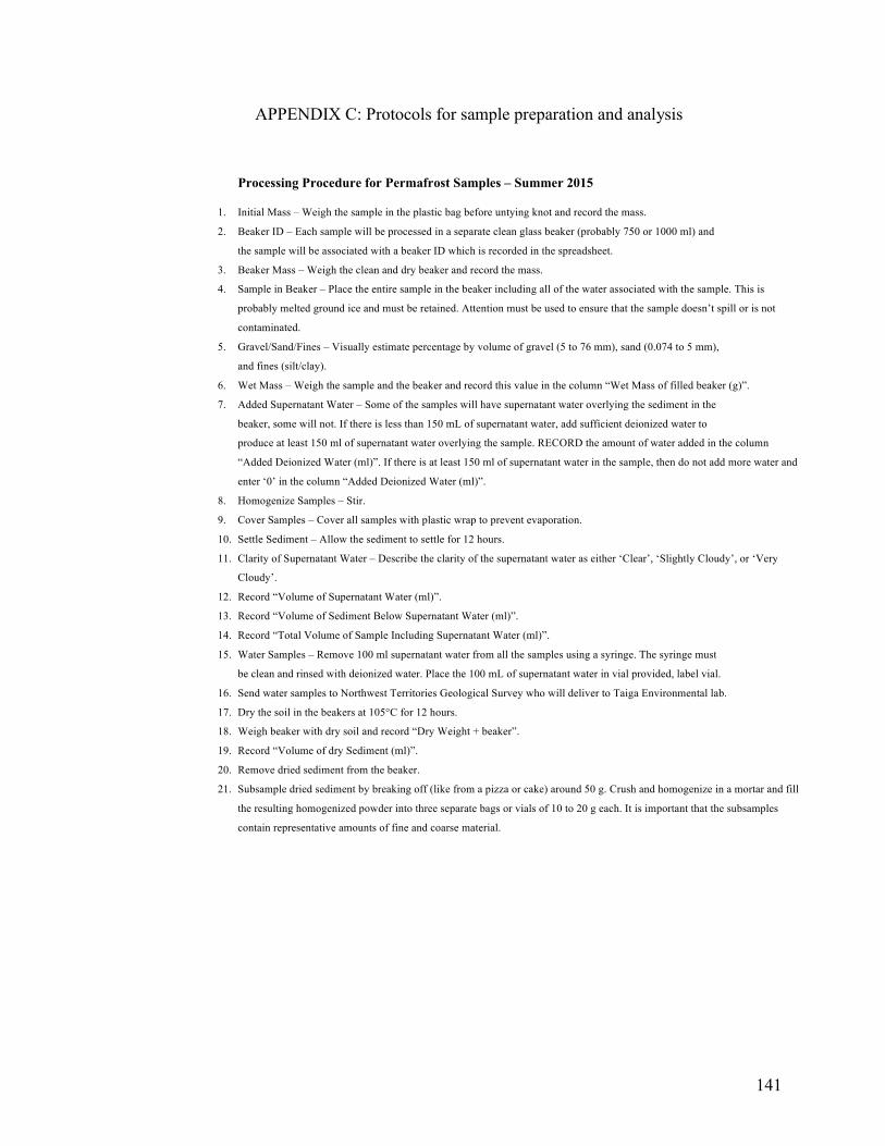
141
APPENDIX C: Protocols for sample preparation and analysis
Processing Procedure for Permafrost Samples – Summer 2015
1. Initial Mass – Weigh the sample in the plastic bag before untying knot and record the mass.
2. Beaker ID – Each sample will be processed in a separate clean glass beaker (probably 750 or 1000 ml) and
the sample will be associated with a beaker ID which is recorded in the spreadsheet.
3. Beaker Mass – Weigh the clean and dry beaker and record the mass.
4. Sample in Beaker – Place the entire sample in the beaker including all of the water associated with the sample. This is
probably melted ground ice and must be retained. Attention must be used to ensure that the sample doesn’t spill or is not
contaminated.
5. Gravel/Sand/Fines – Visually estimate percentage by volume of gravel (5 to 76 mm), sand (0.074 to 5 mm),
and fines (silt/clay).
6. Wet Mass – Weigh the sample and the beaker and record this value in the column “Wet Mass of filled beaker (g)”.
7. Added Supernatant Water – Some of the samples will have supernatant water overlying the sediment in the
beaker, some will not. If there is less than 150 mL of supernatant water, add sufficient deionized water to
produce at least 150 ml of supernatant water overlying the sample. RECORD the amount of water added in the column
“Added Deionized Water (ml)”. If there is at least 150 ml of supernatant water in the sample, then do not add more water and
enter ‘0’ in the column “Added Deionized Water (ml)”.
8. Homogenize Samples – Stir.
9. Cover Samples – Cover all samples with plastic wrap to prevent evaporation.
10. Settle Sediment – Allow the sediment to settle for 12 hours.
11. Clarity of Supernatant Water – Describe the clarity of the supernatant water as either ‘Clear’, ‘Slightly Cloudy’, or ‘Very
Cloudy’.
12. Record “Volume of Supernatant Water (ml)”.
13. Record “Volume of Sediment Below Supernatant Water (ml)”.
14. Record “Total Volume of Sample Including Supernatant Water (ml)”.
15. Water Samples – Remove 100 ml supernatant water from all the samples using a syringe. The syringe must
be clean and rinsed with deionized water. Place the 100 mL of supernatant water in vial provided, label vial.
16. Send water samples to Northwest Territories Geological Survey who will deliver to Taiga Environmental lab.
17. Dry the soil in the beakers at 105°C for 12 hours.
18. Weigh beaker with dry soil and record “Dry Weight + beaker”.
19. Record “Volume of dry Sediment (ml)”.
20. Remove dried sediment from the beaker.
21. Subsample dried sediment by breaking off (like from a pizza or cake) around 50 g. Crush and homogenize in a mortar and fill
the resulting homogenized powder into three separate bags or vials of 10 to 20 g each. It is important that the subsamples
contain representative amounts of fine and coarse material.

142
APPENDIX D: Data
1. Control Group
Field data from the Control group representing the surface conditions
BoreholeID
(NGO-
DD15-
Easting
(m)
Northing
(m)
Elevation
(m)
Terrain
Type
Surface
Topography
Vegetation
1006 536691 7164515 439 Peatland Hummocky Shrubs,
Grasses,
Sedges,
Mosses
1007 536712 7164515 439 Peatland Hummocky Shrubs,
Grasses,
Sedges,
Mosses
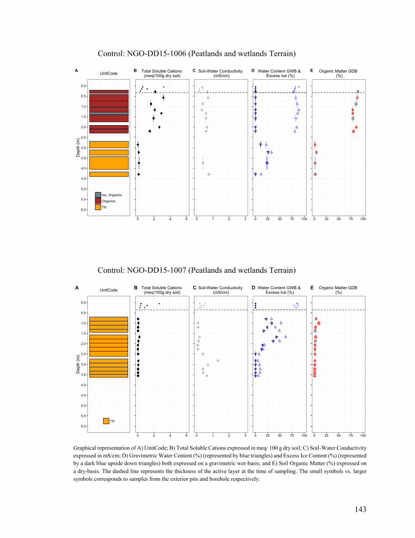
143
Control: NGO-DD15-1006 (Peatlands and wetlands Terrain)
Control: NGO-DD15-1007 (Peatlands and wetlands Terrain)
Graphical representation of A) UnitCode; B) Total Soluble Cations expressed in meq/ 100 g dry soil; C) Soil-Water Conductivity
expressed in mS/cm; D) Gravimetric Water Content (%) (represented by blue triangles) and Excess Ice Content (%) (represented
by a dark blue upside down triangles) both expressed on a gravimetric wet-basis; and E) Soil Organic Matter (%) expressed on
a dry-basis. The dashed line represents the thickness of the active layer at the time of sampling. The small symbols vs. larger
symbols corresponds to samples from the exterior pits and borehole respectively.
0.0
0.5
1.0
1.5
2.0
2.5
3.0
3.5
4.0
4.5
5.0
5.5
6.0
Depth
(m
)
Ice, Organics
Organics
Till
UnitCodeA
0 2 4 6
Total Soluble Cations (meq/100g dry soil)
B
0 1 2 3
Soil-Water Conductivity (mS/cm)
C
0 25 50 75 100
Water Content GWB & Excess Ice (%)
D
0 25 50 75 100
Organic Matter GDB (%)
E
0.0
0.5
1.0
1.5
2.0
2.5
3.0
3.5
4.0
4.5
5.0
5.5
6.0
Depth
(m
)
Till
UnitCodeA
0 2 4 6
Total Soluble Cations (meq/100g dry soil)
B
0 1 2 3
Soil-Water Conductivity (mS/cm)
C
0 25 50 75 100
Water Content GWB & Excess Ice (%)
D
0 25 50 75 100
Organic Matter GDB (%)
E

144
2. Hill 1 Group
Field data from Hill 1 group representing the surface conditions
BoreholeID
(NGO-
DD15-
Easting
(m)
Northing
(m)
Elevation
(m)
Terrain
Type
Surface
Topography
Vegetation
1004 536470
7163553
471
Steep Slope
(SouthFace)
Hilly Shrubs,
Lichens,
Mosses
2004 536548
7163683
480 Top of Hill Hilly Shrubs,
Lichens,
Mosses
2005 536707
7163726
472 Steep Slope
(EastFace)
Hilly (Gentle
slope)
Shrubs,
Lichens,
Mosses
2006 536825
7163749
453 Hill Bottom
(EastFace)
Hilly
(Steep slope)
Shrubs,
Sedges,
Lichens,
Mosses
2007 536591
7163926
459 Steep Slope
(NorthFace)
Hilly Shrubs,
Lichens,
Mosses
1005 536587
7164081
440 Peatland Hummocky Shrubs,
Grasses,
Sedges,
Lichens

145
Hill 1: NGO-DD15-1004 (Till Blanket Terrain)
Hill 1: NGO-DD15-2004 (Till Blanket Terrain)
Graphical representation of A) UnitCode; B) Total Soluble Cations expressed in meq/ 100 g dry soil; C) Soil-Water Conductivity
expressed in mS/cm; D) Gravimetric Water Content (%) (represented by blue triangles) and Excess Ice Content (%) (represented
by a dark blue upside down triangles) both expressed on a gravimetric wet-basis; and E) Soil Organic Matter (%) expressed on
a dry-basis. The dashed line represents the thickness of the active layer at the time of sampling. The small symbols vs. larger
symbols corresponds to samples from the exterior pits and borehole respectively.
0.0
0.5
1.0
1.5
2.0
2.5
3.0
3.5
4.0
4.5
5.0
5.5
6.0
Depth
(m
)
Organics
Organics, Till
Till
UnitCodeA
0 2 4 6
Total Soluble Cations (meq/100g dry soil)
B
0 3 6 9
Soil-Water Conductivity (mS/cm)
C
0 25 50 75 100
Water Content GWB (%)
D
0 25 50 75 100
Organic Matter GDB (%)
E
0.0
0.5
1.0
1.5
2.0
2.5
3.0
3.5
4.0
4.5
5.0
5.5
6.0
Depth
(m
)
Gravel/Cobbles
Ice
Till
Till, Ice
UnitCodeA
0 2 4 6
Total Soluble Cations (meq/100g dry soil)
B
0 2 4 6
Soil-Water Conductivity (mS/cm)
C
0 25 50 75 100
Water Content GWB & Excess Ice (%)
D
0 25 50 75 100
Organic Matter GDB (%)
E
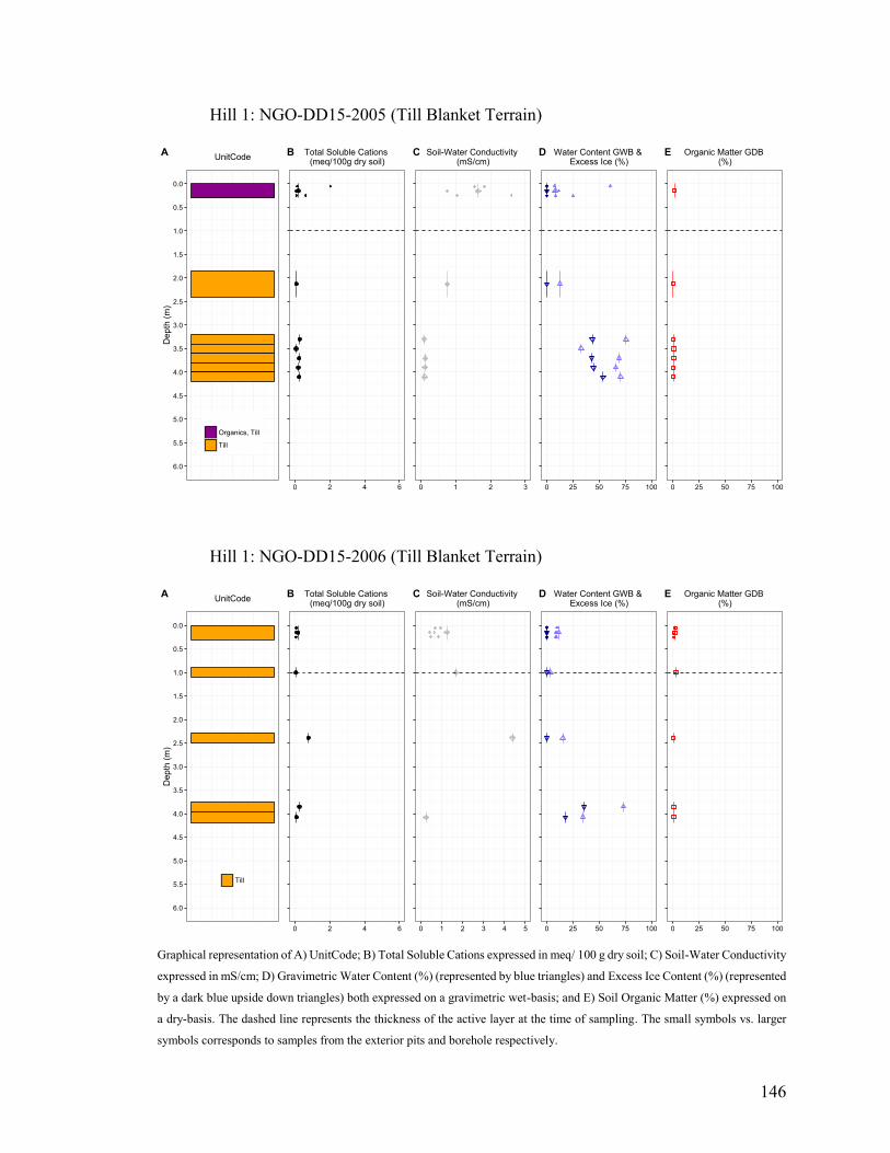
146
Hill 1: NGO-DD15-2005 (Till Blanket Terrain)
Hill 1: NGO-DD15-2006 (Till Blanket Terrain)
Graphical representation of A) UnitCode; B) Total Soluble Cations expressed in meq/ 100 g dry soil; C) Soil-Water Conductivity
expressed in mS/cm; D) Gravimetric Water Content (%) (represented by blue triangles) and Excess Ice Content (%) (represented
by a dark blue upside down triangles) both expressed on a gravimetric wet-basis; and E) Soil Organic Matter (%) expressed on
a dry-basis. The dashed line represents the thickness of the active layer at the time of sampling. The small symbols vs. larger
symbols corresponds to samples from the exterior pits and borehole respectively.
0.0
0.5
1.0
1.5
2.0
2.5
3.0
3.5
4.0
4.5
5.0
5.5
6.0
Depth
(m
)
Organics, Till
Till
UnitCodeA
0 2 4 6
Total Soluble Cations (meq/100g dry soil)
B
0 1 2 3
Soil-Water Conductivity (mS/cm)
C
0 25 50 75 100
Water Content GWB & Excess Ice (%)
D
0 25 50 75 100
Organic Matter GDB (%)
E
0.0
0.5
1.0
1.5
2.0
2.5
3.0
3.5
4.0
4.5
5.0
5.5
6.0
Depth
(m
)
Till
UnitCodeA
0 2 4 6
Total Soluble Cations (meq/100g dry soil)
B
0 1 2 3 4 5
Soil-Water Conductivity (mS/cm)
C
0 25 50 75 100
Water Content GWB & Excess Ice (%)
D
0 25 50 75 100
Organic Matter GDB (%)
E
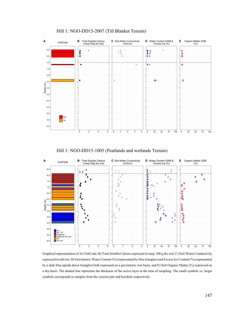
147
Hill 1: NGO-DD15-2007 (Till Blanket Terrain)
Hill 1: NGO-DD15-1005 (Peatlands and wetlands Terrain)
Graphical representation of A) UnitCode; B) Total Soluble Cations expressed in meq/ 100 g dry soil; C) Soil-Water Conductivity
expressed in mS/cm; D) Gravimetric Water Content (%) (represented by blue triangles) and Excess Ice Content (%) (represented
by a dark blue upside down triangles) both expressed on a gravimetric wet-basis; and E) Soil Organic Matter (%) expressed on
a dry-basis. The dashed line represents the thickness of the active layer at the time of sampling. The small symbols vs. larger
symbols corresponds to samples from the exterior pits and borehole respectively.
0.0
0.5
1.0
1.5
2.0
2.5
3.0
3.5
4.0
4.5
5.0
5.5
6.0
Depth
(m
)
Soil
Till
UnitCodeA
0 2 4 6
Total Soluble Cations (meq/100g dry soil)
B
0 1 2 3 4
Soil-Water Conductivity (mS/cm)
C
0 25 50 75 100
Water Content GWB & Excess Ice (%)
D
0 25 50 75 100
Organic Matter GDB (%)
E
0.0
0.5
1.0
1.5
2.0
2.5
3.0
3.5
4.0
4.5
5.0
5.5
6.0
Depth
(m
)
IceIce, TillOrganicsOrganics,Till, IceTillTill, Ice
UnitCodeA
0 2 4 6
Total Soluble Cations (meq/100g dry soil)
B
0 1 2 3
Soil-Water Conductivity (mS/cm)
C
0 25 50 75 100
Water Content GWB & Excess Ice (%)
D
0 25 50 75 100
Organic Matter GDB (%)
E

148
3. Hill 2 Group
Field data from Hill 2 group representing the surface conditions
BoreholeID
(NGO-
DD15-
Easting
(m)
Northing
(m)
Elevation
(m)
Terrain
Type
Surface
Topography
Vegetation
1014 512651
7166738
489 Top of Hill Not Available Not
Available
2018 526886
7176651
461
Low-lying
Depression
Hummocky Shrubs,
Sedges,
Mosses

149
Hill 2: NGO-DD15-1014 (Till Veneer Terrain)
Hill 2: NGO-DD15-2018 (Till Veneer Terrain)
Graphical representation of A) UnitCode; B) Total Soluble Cations expressed in meq/ 100 g dry soil; C) Soil-Water Conductivity
expressed in mS/cm; D) Gravimetric Water Content (%) (represented by blue triangles) and Excess Ice Content (%) (represented
by a dark blue upside down triangles) both expressed on a gravimetric wet-basis; and E) Soil Organic Matter (%) expressed on
a dry-basis. The dashed line represents the thickness of the active layer at the time of sampling. The small symbols vs. larger
symbols corresponds to samples from the exterior pits and borehole respectively.
0.0
0.5
1.0
1.5
2.0
2.5
3.0
3.5
4.0
4.5
5.0
5.5
6.0
6.5
7.0
7.5
8.0
8.5
9.0
9.5
10.0
Depth
(m
)
Till
Till, Ice
UnitCodeA
0 2 4 6
Total Soluble Cations (meq/100g dry soil)
B
0 1 2 3
Soil-Water Conductivity (mS/cm)
C
0 25 50 75 100
Water Content GWB & Excess Ice (%)
D
0 25 50 75 100
Organic Matter GDB (%)
E
0.0
0.5
1.0
1.5
2.0
2.5
3.0
3.5
4.0
4.5
5.0
5.5
6.0
Depth
(m
)
Sand, Silt
Soil
Till
UnitCodeA
0 2 4 6
Total Soluble Cations (meq/100g dry soil)
B
0 1 2 3
Soil-Water Conductivity (mS/cm)
C
0 25 50 75 100
Water Content GWB & Excess Ice (%)
D
0 25 50 75 100
Organic Matter GDB (%)
E

150
4. Hill 3 Group
Field data from Hill 3 group representing the surface conditions
BoreholeID
(NGO-
DD15-
Easting
(m)
Northing
(m)
Elevation
(m)
Terrain
Type
Surface
Topography
Vegetation
2033 537552 7164712 458 Top of Hill Hummocky Shrubs,
Grasses,
Mosses,
Lichens
2009 537477 7164566 446 Hill Bottom
(SouthFace)
Hummocky Shrubs,
Grasses,
Mosses,
Lichens

151
Hill 3: NGO-DD15-2033 (Till Blanket Terrain)
Hill 3: NGO-DD15-2009 (Till Blanket Terrain)
Graphical representation of A) UnitCode; B) Total Soluble Cations expressed in meq/ 100 g dry soil; C) Soil-Water Conductivity
expressed in mS/cm; D) Gravimetric Water Content (%) (represented by blue triangles) and Excess Ice Content (%) (represented
by a dark blue upside down triangles) both expressed on a gravimetric wet-basis; and E) Soil Organic Matter (%) expressed on
a dry-basis. The dashed line represents the thickness of the active layer at the time of sampling. The small symbols vs. larger
symbols corresponds to samples from the exterior pits and borehole respectively.
0.0
0.5
1.0
1.5
2.0
2.5
3.0
3.5
4.0
4.5
5.0
5.5
6.0
Depth
(m
)
Till
UnitCodeA
0 2 4 6
Total Soluble Cations (meq/100g dry soil)
B
0 1 2 3
Soil-Water Conductivity (mS/cm)
C
0 25 50 75 100
Water Content GWB & Excess Ice (%)
D
0 25 50 75 100
Organic Matter GDB (%)
E
0.0
0.5
1.0
1.5
2.0
2.5
3.0
3.5
4.0
4.5
5.0
5.5
6.0
Depth
(m
)
Soil
Till
UnitCodeA
0 2 4 6
Total Soluble Cations (meq/100g dry soil)
B
0 1 2 3
Soil-Water Conductivity (mS/cm)
C
0 25 50 75 100
Water Content GWB & Excess Ice (%)
D
0 25 50 75 100
Organic Matter GDB (%)
E

152
5. Valley Group
Field data from the Valley group representing the surface conditions
BoreholeID
(NGO-
DD15-
Easting
(m)
Northing
(m)
Elevation
(m)
Terrain
Type
Surface
Topography
Vegetation
2013 525915
7175659 440
Hill Bottom,
Snow Drifts
Hummocky Shrubs,
Sedges,
Mosses,
Lichens
2011 526327
7175398 432
Wetland Hummocky Shrubs,
Sedges,
Mosses
2012 526341 7175331
433
Wetland Hummocky Shrubs,
Sedges,
Mosses,
Lichens
1009 526480 7175266
432
Peatland Hummocky Shrubs,
Sedges,
Lichens
2019 526910 7175377
428 Hill Bottom,
Snow Drifts
Hilly Shrubs,
Sedges,
Mosses
1010 526708 7175445 426
Wetland Hummocky Shrubs,
Sedges,
Mosses,
Lichens
2015 526747 7175566
425 Peatland Hummocky Shrubs,
Sedges,
Mosses,
Lichens
2016 526649 7175677 431 Hill Bottom Hummocky Shrubs,
Lichens

153
Valley: NGO-DD15-2013 (Till Veneer Terrain)
Valley: NGO-DD15-2011 (Peatlands and wetlands Terrain)
Graphical representation of A) UnitCode; B) Total Soluble Cations expressed in meq/ 100 g dry soil; C) Soil-Water Conductivity
expressed in mS/cm; D) Gravimetric Water Content (%) (represented by blue triangles) and Excess Ice Content (%) (represented
by a dark blue upside down triangles) both expressed on a gravimetric wet-basis; and E) Soil Organic Matter (%) expressed on
a dry-basis. The dashed line represents the thickness of the active layer at the time of sampling. The small symbols vs. larger
symbols corresponds to samples from the exterior pits and borehole respectively.
0.0
0.5
1.0
1.5
2.0
2.5
3.0
3.5
4.0
4.5
5.0
5.5
6.0
Depth
(m
)
Till
UnitCodeA
0 2 4 6
Total Soluble Cations (meq/100g dry soil)
B
0 1 2 3
Soil-Water Conductivity (mS/cm)
C
0 25 50 75 100
Water Content GWB & Excess Ice (%)
D
0 25 50 75 100
Organic Matter GDB (%)
E
0.0
0.5
1.0
1.5
2.0
2.5
3.0
3.5
4.0
4.5
5.0
5.5
6.0
Depth
(m
)
SoilTill
UnitCodeA
0 2 4 6
Total Soluble Cations (meq/100g dry soil)
B
0 2 4 6
Soil-Water Conductivity (mS/cm)
C
0 25 50 75 100
Water Content GWB & Excess Ice (%)
D
0 25 50 75 100
Organic Matter GDB (%)
E

154
Valley: NGO-DD15-2012 (Peatlands and wetlands Terrain)
Valley: NGO-DD15-1009 (Peatlands and wetlands Terrain)
Graphical representation of A) UnitCode; B) Total Soluble Cations expressed in meq/ 100 g dry soil; C) Soil-Water Conductivity
expressed in mS/cm; D) Gravimetric Water Content (%) (represented by blue triangles) and Excess Ice Content (%) (represented
by a dark blue upside down triangles) both expressed on a gravimetric wet-basis; and E) Soil Organic Matter (%) expressed on
a dry-basis. The dashed line represents the thickness of the active layer at the time of sampling. The small symbols vs. larger
symbols corresponds to samples from the exterior pits and borehole respectively.
0.0
0.5
1.0
1.5
2.0
2.5
3.0
3.5
4.0
4.5
5.0
5.5
6.0
De
pth
(m
)
Till
UnitCodeA
0 2 4 6
Total Soluble Cations (meq/100g dry soil)
B
0 1 2 3
Soil-Water Conductivity (mS/cm)
C
0 25 50 75 100
Water Content GWB & Excess Ice (%)
D
0 25 50 75 100
Organic Matter GDB (%)
E
0.0
0.5
1.0
1.5
2.0
2.5
3.0
3.5
4.0
4.5
5.0
5.5
6.0
Depth
(m
)
Ice
Organics, Sand
Till
UnitCodeA
0 2 4 6
Total Soluble Cations (meq/100g dry soil)
B
0 1 2 3
Soil-Water Conductivity (mS/cm)
C
0 25 50 75 100
Water Content GWB & Excess Ice (%)
D
0 25 50 75 100
Organic Matter GDB (%)
E

155
Valley: NGO-DD15-2019 (Till Veneer Terrain)
Valley: NGO-DD15-1010 (Peatlands and wetlands Terrain)
Graphical representation of A) UnitCode; B) Total Soluble Cations expressed in meq/ 100 g dry soil; C) Soil-Water Conductivity
expressed in mS/cm; D) Gravimetric Water Content (%) (represented by blue triangles) and Excess Ice Content (%) (represented
by a dark blue upside down triangles) both expressed on a gravimetric wet-basis; and E) Soil Organic Matter (%) expressed on
a dry-basis. The dashed line represents the thickness of the active layer at the time of sampling. The small symbols vs. larger
symbols corresponds to samples from the exterior pits and borehole respectively.
0.0
0.5
1.0
1.5
2.0
2.5
3.0
3.5
4.0
4.5
5.0
5.5
6.0
De
pth
(m
)
Till
UnitCodeA
0 2 4 6
Total Soluble Cations (meq/100g dry soil)
B
0 1 2 3
Soil-Water Conductivity (mS/cm)
C
0 25 50 75 100
Water Content GWB & Excess Ice (%)
D
0 25 50 75 100
Organic Matter GDB (%)
E
0.0
0.5
1.0
1.5
2.0
2.5
3.0
3.5
4.0
4.5
5.0
5.5
6.0
Depth
(m
)
IceOrganicsSiltTill
UnitCodeA
0.0 2.5 5.0 7.5 10.0
Total Soluble Cations (meq/100g dry soil)
B
0 1 2 3 4 5
Soil-Water Conductivity (mS/cm)
C
0 25 50 75 100
Water Content GWB & Excess Ice (%)
D
0 25 50 75 100
Organic Matter GDB (%)
E

156
Valley: NGO-DD15-2015 (Peatlands and wetlands Terrain)
Valley: NGO-DD15-2016 (Till Veneer Terrain)
Graphical representation of A) UnitCode; B) Total Soluble Cations expressed in meq/ 100 g dry soil; C) Soil-Water Conductivity
expressed in mS/cm; D) Gravimetric Water Content (%) (represented by blue triangles) and Excess Ice Content (%) (represented
by a dark blue upside down triangles) both expressed on a gravimetric wet-basis; and E) Soil Organic Matter (%) expressed on
a dry-basis. The dashed line represents the thickness of the active layer at the time of sampling. The small symbols vs. larger
symbols corresponds to samples from the exterior pits and borehole respectively.
0.0
0.5
1.0
1.5
2.0
2.5
3.0
3.5
4.0
4.5
5.0
5.5
6.0
Depth
(m
)
Till
UnitCodeA
0 2 4 6
Total Soluble Cations (meq/100g dry soil)
B
0 1 2 3
Soil-Water Conductivity (mS/cm)
C
0 25 50 75 100
Water Content GWB & Excess Ice (%)
D
0 25 50 75 100
Organic Matter GDB (%)
E
0.0
0.5
1.0
1.5
2.0
2.5
3.0
3.5
4.0
4.5
5.0
5.5
6.0
Depth
(m
)
Sand, Soil
Till
UnitCodeA
0 2 4 6
Total Soluble Cations (meq/100g dry soil)
B
0 1 2 3
Soil-Water Conductivity (mS/cm)
C
0 25 50 75 100
Water Content GWB (%)
D
0 25 50 75 100
Organic Matter GDB (%)
E

157
6. Esker 1 Group
Field data from the Esker 1 group representing the surface conditions
BoreholeID
(NGO-
DD15-
Easting
(m)
Northing
(m)
Elevation
(m)
Terrain
Type
Surface
Topography
Vegetation
2008 539002
7164161
458 Esker Hunmocky Shrubs,
Lichens
2028 539001
7164157
458 Esker Hummocky Shrubs,
Lichens
2029 539024
7164143 458 Esker Hummocky Shrubs,
Lichens

158
Esker 1: NGO-DD15-2008 (Esker Terrain)
Esker 1: NGO-DD15-2028 (Esker Terrain)
Graphical representation of A) UnitCode; B) Total Soluble Cations expressed in meq/ 100 g dry soil; C) Soil-Water Conductivity
expressed in mS/cm; D) Gravimetric Water Content (%) (represented by blue triangles) expressed on a wet-basis; and E) Soil
Organic Matter (%) expressed on a dry-basis. The small symbols vs. larger symbols corresponds to samples from the exterior
pits and borehole respectively.
0
1
2
3
4
5
6
7
8
9
10
11
12
Depth
(m
)
Soil
Till
UnitCodeA
0 2 4 6
Total Soluble Cations (meq/100g dry soil)
B
0 1 2 3
Soil-Water Conductivity (mS/cm)
C
0 25 50 75 100
Water Content GWB (%)
D
0 25 50 75 100
Organic Matter GDB (%)
E
0
1
2
3
4
5
6
7
8
9
10
11
12
Depth
(m
)
Gravel/Cobbles, SandSand
UnitCodeA
0 2 4 6
Total Soluble Cations (meq/100g dry soil)
B
0 1 2 3
Soil-Water Conductivity (mS/cm)
C
0 25 50 75 100
Water Content GWB (%)
D
0 25 50 75 100
Soil Organic Matter (%)
E

159
Esker 1: NGO-DD15-2029 (Esker Terrain)
Graphical representation of A) UnitCode; B) Total Soluble Cations expressed in meq/ 100 g dry soil; C) Soil-Water Conductivity
expressed in mS/cm; D) Gravimetric Water Content (%) (represented by blue triangles) expressed on a wet-basis; and E) Soil
Organic Matter (%) expressed on a dry-basis. The small symbols vs. larger symbols corresponds to samples from the exterior
pits and borehole respectively.
0
1
2
3
4
5
6
7
8
9
10
11
12
Depth
(m
)
Sand
UnitCodeA
0 2 4 6
Total Soluble Cations (meq/100g dry soil)
B
0 1 2 3
Soil-Water Conductivity (mS/cm)
C
0 25 50 75 100
Water Content GWB (%)
D
0 25 50 75 100
Organic Matter GDB (%)
E

160
7. Esker 2 Group
Field data from the Esker 2 group representing the surface conditions
BoreholeID
(NGO-
DD15-
Easting
(m)
Northing
(m)
Elevation
(m)
Terrain
Type
Surface
Topography
Vegetation
2026 531203 7177920 437 Esker Hilly Shrubs,
Grasses,
Sedges,
Mosses

161
Esker 2: NGO-DD16-2026 (Esker Terrain)
Graphical representation of A) UnitCode; B) Total Soluble Cations expressed in meq/ 100 g dry soil; C) Soil-Water Conductivity
expressed in mS/cm; D) Gravimetric Water Content (%) (represented by blue triangles) expressed on a wet-basis; and E) Soil
Organic Matter (%) expressed on a dry-basis. The small symbols vs. larger symbols corresponds to samples from the exterior
pits and borehole respectively.
0
1
2
3
4
5
6
7
8
9
10
11
12
Depth
(m
)
Silt
UnitCodeA
0 2 4 6
Total Soluble Cations (meq/100g dry soil)
B
0 1 2 3
Soil-Water Conductivity (mS/cm)
C
0 25 50 75 100
Water Content GWB (%)
D
0 25 50 75 100
Organic Matter GDB (%)
E

162
APPENDIX E: Grain size analysis of active layer and permafrost samples from various
terrain types near Lac de Gras, N.W.T.
Terrain Type Sample ID Depth (m) Mean Grain Size (µm) Sand (%) Silt (%) Clay (%)
Peatlands and wetlands 1006-03 0.72–1.03 12 9 83 8
1006-09 2.70–3.00 207 83 15 2 1006-11 3.42–4.05 64 54 41 5
1007-01 0.70–0.90 210 83 15 2
1007-10 2.73–2.93 269 86 13 2
1007-14 3.48–3.63 142 77 21 2
1005-03 0.75–0.95 16 21 70 9
1005-17 2.86–3.03 19 21 72 7
1005-24 3.99–4.16 11 11 79 10
2011-01 0.30–0.48 75 65 33 2
2011-06 1.42–1.62 21 17 78 6
2011-10 2.45–2.65 40 39 57 4
2011-15 3.45–3.65 80 68 30 2
2012-01 0.97–1.25 111 70 28 2 2012-02 1.40–1.60 132 77 21 2
2012-06 2.25–2.50 63 58 39 2
2012-09 3.40–3.60 45 39 57 4
1009-01 0.00–0.28 142 76 22 2
1009-06 1.56–1.76 108 66 32 2
1009-11 2.50–2.70 88 67 31 2
1009-14 3.10–3.40 20 15 79 6
1010-02 0.15–0.42 6 4 81 15
1010-06 1.52–1.71 38 45 49 6
1010-11 2.58–2.78 165 80 18 2 1010-15 3.40–3.50 27 38 54 7
2015-01 0.95–1.15 52 49 47 4 2015-03 1.35–1.55 89 67 31 2
Mean 83 51 44 4
SD 68 26 23 3
Till Blanket 1004-02 0.20–0.40 84 61 33 6
1004-10 3.96–4.08 135 74 23 3
2004-01 0.10–0.60 188 82 17 2 2004-05 1.82–2.70 172 82 17 2
2004-06 3.45–3.95 124 72 25 3
2005-01 0.00–0.30 107 69 28 3
2005-04 1.85–2.40 285 94 6 1
2005-07 3.60–3.80 152 77 21 2
2006-03 2.28–2.50 241 93 6 1
2006-04 3.75–3.95 201 83 15 2
2007-01 0.00–0.20 247 90 9 1
2007-05 2.31–2.50 198 83 16 2
2033-01 0.35–0.40 87 73 23 4
2033-03 3.85–4.10 136 74 23 3
2009-01 0.00–0.30 274 90 9 1
2009-03 2.80–3.90 289 90 9 1
Mean 182 80 17 2
SD 67 9 8 1
Till Veneer 1014-01 4.03–4.23 139 73 25 2
2018-02 0.30–0.40 217 86 13 1
2018-08 2.65–2.80 168 82 16 1
2013-01 1.80–2.00 98 57 40 3
2013-03 2.20–2.50 17 12 83 5
2016-01 0.00–0.34 100 76 22 2
2019-01 1.80–2.00 43 46 49 5
2019-04 2.40–2.60 15 15 77 8
Mean 100 56 41 4
SD 68 27 25 2
Eskers 2008-01 0.00–0.30 238 95 4 1
2028-01 0.00–0.30 238 91 8 1
2028-04 9.00–11.7 132 71 26 3
2029-01 1.50–3.00 238 87 11 1
2029-06 9.00–10.5 214 88 11 1
2026-01 0.00–1.50 64 58 39 3
Mean 212 82 16 2
SD 41 13 16 1

163
APPENDIX F1: Summary statistics of gravimetric water content GWB (%) in the top 0.5 m, 1 m, 2 m, 4 m, 6 m and 10 m of 24 sites near Lac de Gras, N.W.T. N is the number of samples,
PS (%) is the percentage of total sampling that was considered and N/A values delineate depth intervals where no samples were recovered or core lengths that did not reach the specified
depths.
Top 0.5 m Top 1 m Top 2 m
Terrain Core ID
N PS
(%) Mean Median Max Min SD
N PS
(%) Mean Median Max Min SD
N PS
(%) Mean Median Max Min SD
Peatlands and wetlands 1006 7 72 81.3 80.9 89.3 78.0 3.8 9 100 81.9 81.1 89.3 78.0 3.5 12 83 83.0 82.1 89.3 78.0 3.8
1007 6 60 84.2 84.9 86.8 80.0 2.6 7 94 76.9 84.6 86.8 33.0 19.5 12 73 66.0 70.9 86.8 33.0 20.2
1005 7 90 60.3 82.8 85.3 10.6 34.6 9 90 64.2 81.9 85.3 10.6 31.0 13 86 54.7 64.3 85.3 10.6 31.2
2011 7 96 81.4 90.0 92.1 27.7 23.7 9 84 75.6 89.9 92.1 27.7 23.5 14 91 64.2 55.4 92.1 27.1 25.2
2012 6 60 43.8 42.4 76.1 17.4 28.4 0 0 N/A N/A N/A N/A N/A 10 59 40.5 35.3 76.1 17.4 21.8
1009 7 60 81.3 82.2 91.1 59.5 10.8 9 73 73.7 80.4 91.1 45.8 17.8 13 82 70.4 73.7 91.1 45.8 16.0
1010 8 84 77.7 84.7 92.8 45.9 16.9 10 83 75.7 81.4 92.8 45.9 15.9 13 76 70.1 76.8 92.8 39.9 18.0
2015 6 60 20.4 17.9 31.8 16.4 5.9 0 0 N/A N/A N/A N/A N/A 11 68 29.1 29.3 53.2 16.4 13.1
Till Blanket 1004 8 80 8.6 9.2 10.5 5.2 1.7 10 74 7.9 8.4 10.5 4.1 2.2 12 53 7.9 8.4 10.5 4.1 2.0
2004 7 100 23.3 14.7 68.2 8.7 22.3 0 0 N/A N/A N/A N/A N/A 9 56 22.0 14.7 68.2 8.7 19.6
2005 7 60 18.4 8.6 60.7 7.5 19.6 0 0 N/A N/A N/A N/A N/A 0 0 N/A N/A N/A N/A N/A
2006 7 60 9.6 9.6 11.4 8.0 1.1 0 0 N/A N/A N/A N/A N/A 8 25 8.9 9.5 11.4 3.5 2.4
2033 7 70 10.5 9.0 19.5 7.1 4.3 0 0 N/A N/A N/A N/A N/A 0 0 N/A N/A N/A N/A N/A
2007 8 80 16.1 11.0 55.9 7.8 16.1 9 60 15.2 10.9 55.9 7.8 15.3 10 18 14.5 10.5 55.9 7.8 14.6
2009 7 60 10.1 10.2 12.6 6.9 1.8 0 0 N/A N/A N/A N/A N/A 8 25 9.7 9.9 12.6 6.8 2.1
Till Veneer 2018 7 80 74.5 82.9 88.6 24.4 22.6 8 57 72.2 80.1 88.6 24.4 21.9 9 79 70.9 77.3 88.6 24.4 20.9
2019 6 60 39.9 24.0 83.1 14.4 31.7 0 0 N/A N/A N/A N/A N/A 7 25 38.5 26.5 83.1 14.4 29.2
1014 0 0 N/A N/A N/A N/A N/A 0 0 N/A N/A N/A N/A N/A 0 0 N/A N/A N/A N/A N/A
2013 6 60 24.3 15.2 71.7 10.6 23.5 0 0 N/A N/A N/A N/A N/A 7 25 25.3 17.1 71.7 10.6 21.6
2016 7 68 16.6 15.2 27.3 13.0 4.9 8 100 16.8 15.4 27.3 13.0 4.6 0 0 N/A N/A N/A N/A N/A
Eskers 2026 6 60 23.2 24.4 29.1 17.7 4.3 7 100 23.4 24.5 29.1 17.7 4.0 0 0 N/A N/A N/A N/A N/A
2008 7 60 13.8 15.6 20.3 4.4 6.5 0 0 N/A N/A N/A N/A N/A 0 0 N/A N/A N/A N/A N/A
2028 6 60 14.2 16.2 21.8 2.3 7.2 0 0 N/A N/A N/A N/A N/A 7 100 14.7 17.0 21.8 2.3 6.7
2029 6 60 4.7 3.0 10.2 2.1 3.3 0 0 N/A N/A N/A N/A N/A 0 0 N/A N/A N/A N/A N/A
Top 4 m Top 6 m Top 10 m
Core ID
N PS
(%) Mean Median Max Min SD
N PS
(%) Mean Median Max Min SD
N PS
(%) Mean Median Max Min SD
1006 17 80 72.9 81.1 89.3 22.0 22.5 18 58 69.5 81.0 89.3 11.6 26.2 18 0 N/A N/A N/A N/A N/A
1007 20 75 43.5 44.9 86.8 5.2 32.2 0 0 N/A N/A N/A N/A N/A 20 0 N/A N/A N/A N/A N/A
1005 23 83 51.9 53.1 98.7 10.6 30.0 0 0 N/A N/A N/A N/A N/A 26 0 N/A N/A N/A N/A N/A
2011 23 92 49.2 39.3 92.1 20.0 27.6 30 83 42.7 29.0 92.1 19.2 26.9 30 0 N/A N/A N/A N/A N/A
2012 17 65 43.1 42.2 76.1 17.4 17.1 18 46 41.5 42.2 76.1 13.2 18.0 18 0 N/A N/A N/A N/A N/A
1009 21 83 64.9 60.8 91.1 45.8 14.9 0 0 N/A N/A N/A N/A N/A 21 0 N/A N/A N/A N/A N/A
1010 22 83 60.5 56.8 92.8 33.4 19.4 27 74 56.9 54.4 92.8 30.3 19.5 27 0 N/A N/A N/A N/A N/A
2015 0 0 N/A N/A N/A N/A N/A 0 0 N/A N/A N/A N/A N/A 11 0 N/A N/A N/A N/A N/A
1004 15 38 9.4 9.0 25.9 4.1 5.1 17 29 9.5 9.0 25.9 4.1 4.9 17 0 N/A N/A N/A N/A N/A
2004 12 68 33.3 17.7 76.1 8.7 26.5 0 0 N/A N/A N/A N/A N/A 12 0 N/A N/A N/A N/A N/A
2005 12 41 32.1 18.6 75.9 7.5 27.7 13 26 35.1 24.7 75.9 7.5 28.6 13 0 N/A N/A N/A N/A N/A
2006 10 24 15.9 9.6 73.1 3.5 20.3 11 80 17.6 9.6 73.1 3.5 20.1 11 0 N/A N/A N/A N/A N/A
2033 9 17 24.5 9.8 76.1 7.1 28.0 0 0 N/A N/A N/A N/A N/A 12 0 N/A N/A N/A N/A N/A
2007 11 22 16.0 10.9 55.9 7.8 14.7 0 0 N/A N/A N/A N/A N/A 11 0 N/A N/A N/A N/A N/A
2009 9 40 16.2 10.2 68.0 6.8 19.5 0 0 N/A N/A N/A N/A N/A 9 0 N/A N/A N/A N/A N/A
2018 13 83 62.4 60.9 88.6 24.4 22.1 0 0 N/A N/A N/A N/A N/A 13 0 N/A N/A N/A N/A N/A
2019 11 33 36.0 28.9 83.1 14.4 23.4 0 0 N/A N/A N/A N/A N/A 11 0 N/A N/A N/A N/A N/A
1014 0 0 N/A N/A N/A N/A N/A 7 25 78.1 83.6 92.4 52.3 14.6 19 47 71.0 81.8 93.0 24.3 21.1
2013 9 25 25.5 20.3 71.7 10.6 18.8 0 0 N/A N/A N/A N/A N/A 9 0 N/A N/A N/A N/A N/A
2016 0 0 N/A N/A N/A N/A N/A 0 0 N/A N/A N/A N/A N/A 8 0 N/A N/A N/A N/A N/A
2026 0 0 N/A N/A N/A N/A N/A 0 0 N/A N/A N/A N/A N/A 7 0 N/A N/A N/A N/A N/A
2008 8 53 13.3 15.5 20.3 4.4 6.2 9 85 16.5 15.6 41.9 4.4 11.1 9 0 N/A N/A N/A N/A N/A
2028 7 25 14.7 17.0 21.8 2.3 6.7 8 100 15.1 17.3 21.8 2.3 6.3 9 90 15.2 17.0 21.8 2.3 5.9
2029 8 70 6.4 5.3 14.2 2.1 4.5 9 88 7.3 7.2 14.5 2.1 5.0 9 93 9.2 9.8 15.2 2.1 5.4

164
APPENDIX F2: Summary statistics of organic matter content (%) in the top 0.5 m, 1 m, 2 m, 4 m, 6 m and 10 m of 24 sites near Lac de Gras, N.W.T. N is the number of samples, PS (%) is
the percentage of total sampling that was considered and N/A values delineate depth intervals where no samples were recovered or core lengths that did not reach the specified depths.
Top 0.5 m Top 1 m Top 2 m
Terrain Core ID
N PS
(%) Mean Median Max Min SD
N PS
(%) Mean Median Max Min SD
N PS
(%) Mean Median Max Min SD
Peatlands and wetlands 1006 1 32 89.4 89.4 89.4 89.4 N/A 3 77 87.6 87.8 89.4 85.6 1.9 6 54 83.1 82.4 89.4 78.4 5.1
1007 0 0 N/A N/A N/A N/A N/A 1 20 3.5 3.5 3.5 3.5 N/A 6 58 3.7 2.7 9.2 1.8 2.8
1005 1 40 72.5 72.5 72.5 72.5 N/A 3 40 67.5 72.5 80.6 49.3 16.2 9 71 30.8 9.5 80.6 1.0 32.7
2011 1 36 4.8 4.8 4.8 4.8 N/A 3 58 3.9 3.5 4.8 3.5 0.7 8 77 2.5 2.7 4.8 0.9 1.5
2012 0 0 N/A N/A N/A N/A N/A 0 0 N/A N/A N/A N/A N/A 4 44 3.0 2.9 5.3 1.1 1.7
1009 1 56 26.3 26.3 26.3 26.3 N/A 3 87 13.6 10.6 26.3 3.9 11.5 7 81 8.4 4.6 26.3 1.6 8.5
1010 1 54 27.4 27.4 27.4 27.4 N/A 3 68 27.3 27.4 51.8 2.7 24.5 6 69 14.4 2.4 51.8 1.3 21.0
2015 0 0 N/A N/A N/A N/A N/A 0 0 N/A N/A N/A N/A N/A 5 53 1.4 1.2 1.9 1.0 0.4
Till Blanket 1004 8 80 1.7 1.3 4.3 0.9 1.1 10 74 2.2 1.3 7.1 0.9 2.0 12 53 2.3 1.4 7.1 0.9 1.8
2004 1 100 2.8 2.8 2.8 2.8 N/A 0 0 N/A N/A N/A N/A N/A 3 40 1.7 1.2 2.8 1.1 0.9
2005 1 60 1.6 1.6 1.6 1.6 N/A 0 0 N/A N/A N/A N/A N/A 0 0 N/A N/A N/A N/A N/A
2006 7 60 1.5 1.2 3.3 0.7 0.9 0 0 N/A N/A N/A N/A N/A 8 25 1.7 1.3 3.3 0.7 1.0
2033 1 10 2.9 2.9 2.9 2.9 N/A 0 0 N/A N/A N/A N/A N/A 1 0 N/A N/A N/A N/A N/A
2007 2 80 2.1 2.1 2.4 1.8 0.4 3 60 2.1 2.0 2.4 1.8 0.3 4 34 2.0 2.0 2.4 1.8 0.2
2009 7 60 1.1 1.0 2.0 0.4 0.5 7 0 N/A N/A N/A N/A N/A 8 25 1.1 1.0 2.0 0.4 0.5
Till Veneer 2018 1 20 3.9 3.9 3.9 3.9 N/A 2 30 35.0 35.0 66.1 3.9 44.0 3 64 27.4 12.3 66.1 3.9 33.8
2019 0 0 N/A N/A N/A N/A N/A 0 0 N/A N/A N/A N/A N/A 1 10 0.6 0.6 0.6 0.6 N/A
1014 0 0 N/A N/A N/A N/A N/A 0 0 N/A N/A N/A N/A N/A 0 0 N/A N/A N/A N/A N/A
2013 0 0 N/A N/A N/A N/A N/A 0 0 N/A N/A N/A N/A N/A 1 10 1.1 1.1 1.1 1.1 N/A
2016 7 68 2.4 1.7 6.3 1.3 1.8 8 100 2.5 1.8 6.3 1.3 1.7 8 0 N/A N/A N/A N/A N/A
Eskers 2026 6 60 2.9 3.0 5.2 0.8 1.6 7 100 2.8 2.9 5.2 0.8 1.5 0 0 N/A N/A N/A N/A N/A
2008 7 60 4.2 4.0 5.7 2.7 1.0 0 0 N/A N/A N/A N/A N/A 0 0 N/A N/A N/A N/A N/A
2028 0 0 N/A N/A N/A N/A N/A 0 0 N/A N/A N/A N/A N/A 1 100 0.7 0.7 0.7 0.7 N/A
2029 6 60 2.1 1.5 6.2 0.7 2.0 0 0 N/A N/A N/A N/A N/A 0 0 N/A N/A N/A N/A N/A
Top 4 m Top 6 m Top 10 m
Core ID
N PS
(%) Mean Median Max Min SD
N PS
(%) Mean Median Max Min SD
N PS
(%) Mean Median Max Min SD
1006 11 75 61.1 79.1 89.4 1.1 38.0 12 54 56.1 78.7 89.4 1.1 40.1 0 0 N/A N/A N/A N/A N/A
1007 14 68 2.1 1.0 9.2 0.8 2.2 0 0 N/A N/A N/A N/A N/A 0 0 N/A N/A N/A N/A N/A
1005 19 76 15.9 3.0 80.6 0.9 26.2 22 59 14.6 3.6 80.6 0.9 24.5 0 0 N/A N/A N/A N/A N/A
2011 16 86 1.6 0.9 4.8 0.7 1.4 23 78 1.3 0.8 4.8 0.5 1.2 0 0 N/A N/A N/A N/A N/A
2012 11 60 1.9 1.3 5.3 0.9 1.3 12 41 1.8 1.2 5.3 0.9 1.3 0 0 N/A N/A N/A N/A N/A
1009 15 83 4.7 1.8 26.3 1.1 6.6 0 0 N/A N/A N/A N/A N/A 0 0 N/A N/A N/A N/A N/A
1010 15 83 6.7 1.5 51.8 0.7 14.1 20 73 5.4 1.6 51.8 0.7 12.3 0 0 N/A N/A N/A N/A N/A
2015 0 0 N/A N/A N/A N/A N/A 0 0 N/A N/A N/A N/A N/A 0 0 N/A N/A N/A N/A N/A
1004 15 38 2.1 1.3 7.1 0.7 1.7 17 29 1.9 1.3 7.1 0.6 1.6 0 0 N/A N/A N/A N/A N/A
2004 6 67 2.0 1.2 4.8 1.0 1.5 0 0 N/A N/A N/A N/A N/A 0 0 N/A N/A N/A N/A N/A
2005 6 83 0.9 0.8 1.6 0.3 0.4 7 41 0.8 0.7 1.6 0.3 0.4 0 0 N/A N/A N/A N/A N/A
2006 10 24 1.5 1.2 3.3 0.6 0.9 11 80 1.5 1.1 3.3 0.6 0.9 0 0 N/A N/A N/A N/A N/A
2033 3 12 1.7 1.1 2.9 1.1 1.0 6 18 1.4 1.1 2.9 1.0 0.7 0 0 N/A N/A N/A N/A N/A
2007 5 22 2.8 2.0 6.0 1.8 1.8 0 0 N/A N/A N/A N/A N/A 0 0 N/A N/A N/A N/A N/A
2009 9 40 1.1 1.0 2.0 0.4 0.4 0 0 N/A N/A N/A N/A N/A 0 0 N/A N/A N/A N/A N/A
2018 7 51 13.0 2.6 66.1 1.8 23.7 0 0 N/A N/A N/A N/A N/A 0 0 N/A N/A N/A N/A N/A
2019 5 25 0.9 0.8 1.4 0.6 0.3 0 0 N/A N/A N/A N/A N/A 0 0 N/A N/A N/A N/A N/A
1014 0 0 N/A N/A N/A N/A N/A 7 25 1.2 1.2 1.5 1.0 0.2 19 47 1.2 1.1 1.6 1.0 0.2
2013 3 18 1.2 1.2 1.3 1.1 0.1 0 0 N/A N/A N/A N/A N/A 0 0 N/A N/A N/A N/A N/A
2016 8 0 N/A N/A N/A N/A N/A 0 0 N/A N/A N/A N/A N/A 0 0 N/A N/A N/A N/A N/A
2026 0 0 N/A N/A N/A N/A N/A 0 0 N/A N/A N/A N/A N/A 0 0 N/A N/A N/A N/A N/A
2008 8 53 3.8 3.9 5.7 0.9 1.5 9 85 3.4 3.7 5.7 0.4 1.8 0 0 N/A N/A N/A N/A N/A
2028 0 0 N/A N/A N/A N/A N/A 2 100 0.6 0.6 0.7 0.5 0.1 3 90 0.7 0.7 0.9 0.5 0.2
2029 8 70 1.7 1.2 6.2 0.4 1.9 9 88 1.6 0.9 6.2 0.4 1.8 3 93 1.3 0.6 6.2 0.4 1.6

165
APPENDIX F3: Summary statistics of total soluble cations (meq/100 g dry soil) in the top 0.5 m, 1 m, 2 m, 4 m, 6 m and 10 m of 24 sites near Lac de Gras, N.W.T. N is the number of
samples, PS (%) is the percentage of total sampling that was considered and N/A values delineate depth intervals where no samples were recovered or core lengths that did not reach the
specified depths.
Top 0.5 m Top 1 m Top 2 m
Terrain Core ID
N PS
(%) Mean Median Max Min SD
N PS
(%) Mean Median Max Min SD
N PS
(%) Mean Median Max Min SD
Peatlands and wetlands 1006 7 72 1.2 0.6 3.2 0.3 1.1 9 100 1.5 1.2 3.2 0.3 1.2 12 83 1.7 1.8 3.2 0.3 1.1
1007 6 60 0.9 0.6 2.6 0.3 0.9 7 94 0.8 0.4 2.6 0.0 0.9 12 73 0.5 0.2 2.6 0.0 0.8
1005 7 90 0.8 0.7 1.5 0.1 0.6 9 90 1.1 1.4 2.4 0.1 0.8 13 86 0.9 0.7 2.4 0.1 0.8
2011 7 96 3.0 2.9 5.4 0.1 1.6 9 84 2.4 2.9 5.4 0.1 1.8 14 91 1.7 1.0 5.4 0.0 1.7
2012 6 60 0.9 0.7 2.4 0.1 1.0 0 0 N/A N/A N/A N/A N/A 10 59 0.5 0.1 2.4 0.0 0.8
1009 7 60 2.3 2.1 3.4 1.5 0.7 9 73 1.8 2.0 3.4 0.1 1.1 13 82 1.8 2.0 3.4 0.1 1.1
1010 8 84 2.7 2.0 8.1 0.2 2.4 10 83 2.5 2.0 8.1 0.2 2.3 13 76 2.0 1.5 8.1 0.1 2.2
2015 6 60 0.2 0.1 0.6 0.1 0.2 0 0 N/A N/A N/A N/A N/A 11 68 0.2 0.1 0.6 0.1 0.1
Till Blanket 1004 8 80 0.1 0.1 0.1 0.0 0.0 10 74 0.1 0.1 0.1 0.0 0.0 12 53 0.1 0.1 0.3 0.0 0.1
2004 7 100 0.9 0.2 4.9 0.1 1.8 0 0 N/A N/A N/A N/A N/A 9 56 0.8 0.2 4.9 0.1 1.6
2005 7 60 0.5 0.2 2.0 0.1 0.7 0 0 N/A N/A N/A N/A N/A 0 0 N/A N/A N/A N/A N/A
2006 7 60 0.1 0.1 0.2 0.0 0.0 0 0 N/A N/A N/A N/A N/A 8 25 0.1 0.1 0.2 0.0 0.0
2033 7 70 0.1 0.1 0.4 0.0 0.1 0 0 N/A N/A N/A N/A N/A 0 0 N/A N/A N/A N/A N/A
2007 8 80 0.3 0.1 1.9 0.1 0.6 9 60 0.3 0.1 1.9 0.1 0.6 10 18 0.3 0.1 1.9 0.1 0.6
2009 7 60 0.1 0.1 0.1 0.0 0.0 0 0 N/A N/A N/A N/A N/A 8 25 0.1 0.1 0.2 0.0 0.1
Till Veneer 2018 7 80 0.8 0.6 2.2 0.1 0.7 8 57 0.8 0.5 2.2 0.1 0.7 9 79 0.7 0.5 2.2 0.1 0.7
2019 6 60 0.4 0.1 1.8 0.0 0.7 0 0 N/A N/A N/A N/A N/A 7 25 0.4 0.1 1.8 0.0 0.7
1014 0 0 N/A N/A N/A N/A N/A 0 0 N/A N/A N/A N/A N/A 0 0 N/A N/A N/A N/A N/A
2013 6 60 0.3 0.1 1.6 0.1 0.6 0 0 N/A N/A N/A N/A N/A 7 25 0.5 0.1 1.6 0.1 0.7
2016 7 68 0.2 0.1 0.6 0.1 0.2 8 100 0.2 0.1 0.6 0.1 0.2 0 0 N/A N/A N/A N/A N/A
Eskers 2026 6 60 0.1 0.1 0.2 0.0 0.0 7 100 0.1 0.1 0.2 0.0 0.0 0 0 N/A N/A N/A N/A N/A
2008 7 60 0.0 0.0 0.1 0.0 0.0 0 0 N/A N/A N/A N/A N/A 0 0 N/A N/A N/A N/A N/A
2028 6 60 0.1 0.0 0.3 0.0 0.1 0 0 N/A N/A N/A N/A N/A 7 100 0.1 0.0 0.4 0.0 0.2
2029 6 60 0.0 0.0 0.0 0.0 0.0 0 0 N/A N/A N/A N/A N/A 0 0 N/A N/A N/A N/A N/A
Top 4 m Top 6 m Top 10 m
Core ID
N PS
(%) Mean Median Max Min SD
N PS
(%) Mean Median Max Min SD
N PS
(%) Mean Median Max Min SD
1006 17 80 1.4 1.5 3.2 0.0 1.1 18 58 1.4 1.3 3.2 0.0 1.1 0 0 N/A N/A N/A N/A N/A
1007 20
75
0.3 0.1 2.6 0.0 0.6 0
0
N/A N/A N/A N/A N/A 0
0
N/A N/A N/A N/A N/A
1005 23 83 0.8 0.6 2.4 0.1 0.7 26 0 0.8 0.7 2.4 0.1 0.7 0 0 N/A N/A N/A N/A N/A
2011 23 92 1.6 1.2 5.4 0.0 1.4 30 83 1.3 0.5 5.4 0.0 1.4 0 0 N/A N/A N/A N/A N/A
2012 17 65 0.4 0.1 2.4 0.0 0.7 18 46 0.4 0.1 2.4 0.0 0.6 0 0 N/A N/A N/A N/A N/A
1009 21 83 1.5 1.3 3.4 0.1 1.1 0 0 N/A N/A N/A N/A N/A 0 0 N/A N/A N/A N/A N/A
1010 22 83 1.3 0.4 8.1 0.1 1.9 27 74 1.2 0.4 8.1 0.1 1.7 0 0 N/A N/A N/A N/A N/A
2015 0 0 N/A N/A N/A N/A N/A 0 0 N/A N/A N/A N/A N/A 0 0 N/A N/A N/A N/A N/A
1004 15 38 0.2 0.1 0.8 0.0 0.2 17 29 0.2 0.1 0.8 0.0 0.2 0 0 N/A N/A N/A N/A N/A
2004 12 68 0.6 0.3 4.9 0.1 1.4 0 0 N/A N/A N/A N/A N/A 0 0 N/A N/A N/A N/A N/A
2005 12 41 0.3 0.2 2.0 0.1 0.6 13 26 0.3 0.2 2.0 0.1 0.5 0 0 N/A N/A N/A N/A N/A
2006 10 24 0.2 0.1 0.8 0.0 0.2 11 80 0.2 0.1 0.8 0.0 0.2 0 0 N/A N/A N/A N/A N/A
2033 9 17 0.2 0.1 0.4 0.0 0.1 12 0 0.2 0.2 0.4 0.0 0.1 0 0 N/A N/A N/A N/A N/A
2007 11 22 0.3 0.1 1.9 0.0 0.5 0 0 N/A N/A N/A N/A N/A 0 0 N/A N/A N/A N/A N/A
2009 9 40 0.1 0.1 0.5 0.0 0.2 0 0 N/A N/A N/A N/A N/A 0 0 N/A N/A N/A N/A N/A
2018 13 83 0.6 0.3 2.2 0.1 0.6 0 0 N/A N/A N/A N/A N/A 0 0 N/A N/A N/A N/A N/A
2019 11 33 0.4 0.2 1.8 0.0 0.5 0 0 N/A N/A N/A N/A N/A 0 0 N/A N/A N/A N/A N/A
1014 0 0 N/A N/A N/A N/A N/A 7 25 0.4 0.4 1.0 0.1 0.3 19 47 0.4 0.3 1.0 0.1 0.3
2013 9 25 0.7 0.1 1.7 0.1 0.7 0 0 N/A N/A N/A N/A N/A 0 0 N/A N/A N/A N/A N/A
2016 0 0 N/A N/A N/A N/A N/A 0 0 N/A N/A N/A N/A N/A 0 0 N/A N/A N/A N/A N/A
2026 0 0 N/A N/A N/A N/A N/A 0 0 N/A N/A N/A N/A N/A 0 0 N/A N/A N/A N/A N/A
2008 8 53 0.0 0.0 0.1 0.0 0.0 9 85 0.1 0.0 0.2 0.0 0.1 0 0 N/A N/A N/A N/A N/A
2028 0 25 N/A N/A N/A N/A N/A 8 100 0.2 0.1 0.4 0.0 0.2 9 90 0.2 0.2 0.4 0.0 0.2
2029 8 70 0.0 0.0 0.1 0.0 0.0 9 88 0.0 0.0 0.1 0.0 0.0 9 93 0.0 0.1 0.1 0.0 0.0