depreciation in eu member states: empirical and ... · 1 depreciation in eu member states:...

1

Depreciation in EU Member States: Empirical and Methodological Differences 1

Bernd Görzig, DIW Berlin [email protected]

April 2007

Abstract

Depreciation levels in the EU 15 countries vary considerably. However, there seems to be no unique economic factor to explain this. Methodological differences exist, but the causality is not clear-cut. To improve the possibilities of explanation, it would be helpful to apply more standardised methods. The most important strategy for standardisation in the EU KLEMS project is the harmonisation of the asset and industry breakdown. A harmonised asset and industry breakdown will improve the possibilities to separate structural from methodological influences. An open question will remain for the harmonisation of service life assumptions. While it must be conceded that presently differences in service life assumptions across countries might have historical origins, it should also be kept in mind that the service life of an asset is determined by economic factors. These might be different across countries. Depending on the type of asset, service lives might differ.

1 This paper has been prepared for the Helsinki workshop of the EU KLEMS project for Work package 3: Capital Accounts.

2

Contents:

1 Overview.....................................................................................................................................3

2 Economic Explanations of Varying CFC Ratios.........................................................................4

3 The Political Dimension..............................................................................................................6

4 Methodological Differences in Calculating CFC........................................................................9

4.1 Sources of Depreciation Data ...................................................................................................9

4.2 Sources of Capital Stock Data ................................................................................................10

4.3 Service Lives: Definition........................................................................................................14

4.4 Service Lives: Sources ...........................................................................................................15

4.5 Service Lives: Degree of Differentiation................................................................................15

4.6 Service Lives: Comparisons ...................................................................................................16

4.7 Models ....................................................................................................................................22

4.8 Depreciation Schedules ..........................................................................................................22

5 Conclusions for the EU KLEMS Project ..................................................................................23

References:.............................................................................................................................................24

Annex 1: Data Used in Assessing Average Service Lives in the EU Countries ....................................25

Annex 2: Elements of the DIW Capital Stock Model............................................................................27

Tables:

Table 1: Coefficients of Correlation between Selected Indicators and CFC Ratios – Averages 1993 - 2000 ..........................................................................................................................................5

Table 2: Simulation of GDP and Operating Surplus, given equal Shares of CFC in Domestic Product – Averages 1993 – 2000 ................................................................................................7

Table 3: Methods Applied by EU 15 Member States to Calculate Depreciation ..................................11

Table 4: Methods Applied by New Member States to Calculate Depreciation......................................12

Table 5: Stocks and Flows of Fixed Assets according to ESA’95..........................................................14

Table 6: Applied Service Life Assumptions by Selected EU 15 Countries.............................................17

Table 7: Selected Service Life Assumptions by Activity.........................................................................18

Table 8: Assessment of Implicit Service Life Assumptions for Published Depreciation Values - Adaptation Period for CFC 1970 - 2004 ..................................................................................20

Table 9: Ranges of Implicit Service Life for Different Periods .............................................................21

Figures:

Figure 1: CFC Ratios in Net Domestic Product at Factor Costs – Averages 1994 – 2001 ....................3

Figure 2: Share of Operating Surplus in Net Domestic Product – Original and Simulated – Averages 1993 – 2000.................................................................................................................8

3

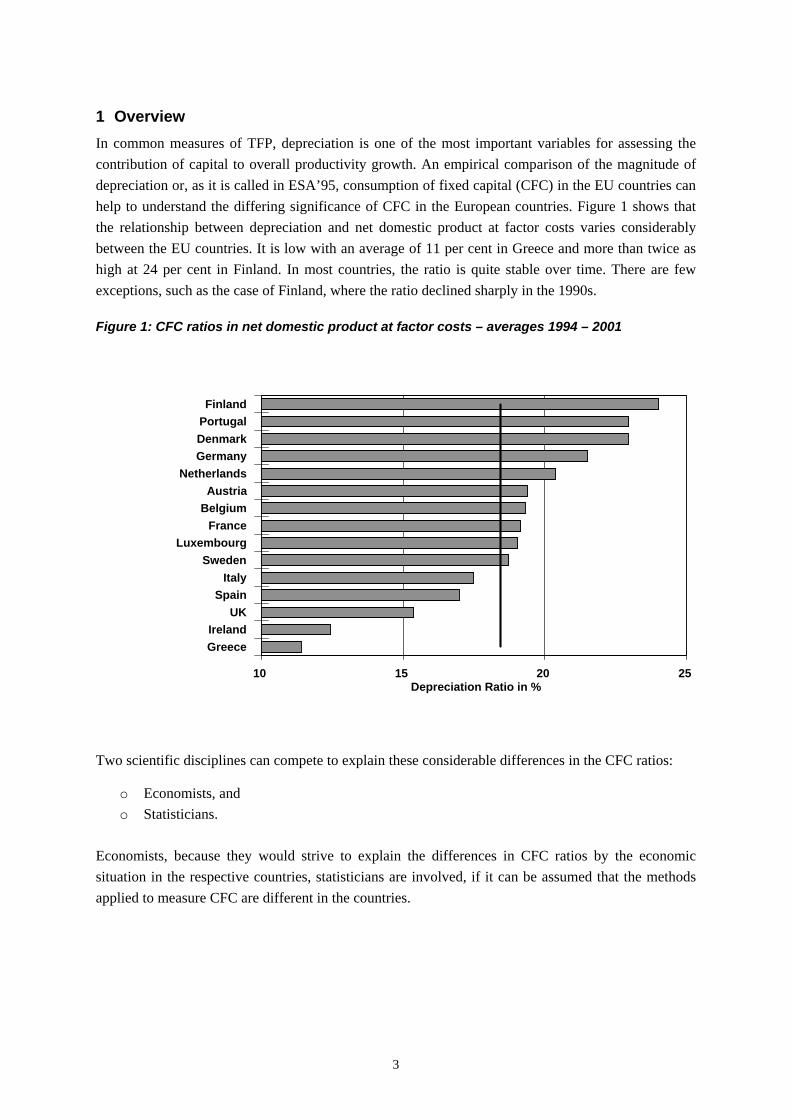
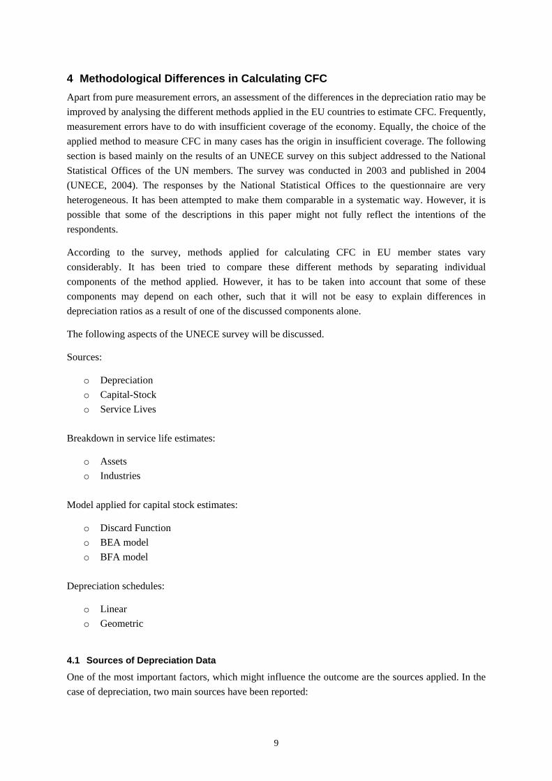
1 Overview In common measures of TFP, depreciation is one of the most important variables for assessing the contribution of capital to overall productivity growth. An empirical comparison of the magnitude of depreciation or, as it is called in ESA’95, consumption of fixed capital (CFC) in the EU countries can help to understand the differing significance of CFC in the European countries. Figure 1 shows that the relationship between depreciation and net domestic product at factor costs varies considerably between the EU countries. It is low with an average of 11 per cent in Greece and more than twice as high at 24 per cent in Finland. In most countries, the ratio is quite stable over time. There are few exceptions, such as the case of Finland, where the ratio declined sharply in the 1990s.

Figure 1: CFC ratios in net domestic product at factor costs – averages 1994 – 2001

Two scientific disciplines can compete to explain these considerable differences in the CFC ratios:

o Economists, and o Statisticians.

Economists, because they would strive to explain the differences in CFC ratios by the economic situation in the respective countries, statisticians are involved, if it can be assumed that the methods applied to measure CFC are different in the countries.

10 15 20 25 Depreciation Ratio in %

GreeceIreland

UKSpain

ItalySweden

LuxembourgFrance

BelgiumAustria

NetherlandsGermanyDenmarkPortugalFinland

4

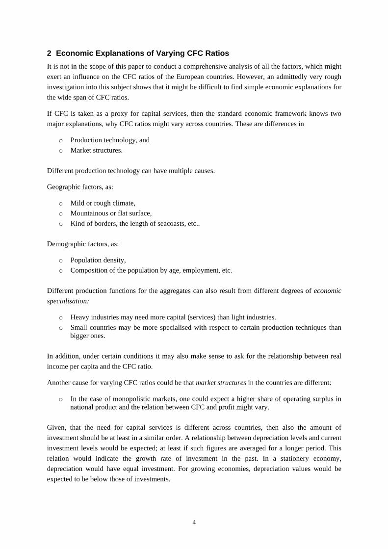
2 Economic Explanations of Varying CFC Ratios It is not in the scope of this paper to conduct a comprehensive analysis of all the factors, which might exert an influence on the CFC ratios of the European countries. However, an admittedly very rough investigation into this subject shows that it might be difficult to find simple economic explanations for the wide span of CFC ratios.

If CFC is taken as a proxy for capital services, then the standard economic framework knows two major explanations, why CFC ratios might vary across countries. These are differences in

o Production technology, and o Market structures.

Different production technology can have multiple causes.

Geographic factors, as:

o Mild or rough climate, o Mountainous or flat surface, o Kind of borders, the length of seacoasts, etc..

Demographic factors, as:

o Population density, o Composition of the population by age, employment, etc.

Different production functions for the aggregates can also result from different degrees of economic specialisation:

o Heavy industries may need more capital (services) than light industries. o Small countries may be more specialised with respect to certain production techniques than

bigger ones.

In addition, under certain conditions it may also make sense to ask for the relationship between real income per capita and the CFC ratio.

Another cause for varying CFC ratios could be that market structures in the countries are different:

o In the case of monopolistic markets, one could expect a higher share of operating surplus in national product and the relation between CFC and profit might vary.

Given, that the need for capital services is different across countries, then also the amount of investment should be at least in a similar order. A relationship between depreciation levels and current investment levels would be expected; at least if such figures are averaged for a longer period. This relation would indicate the growth rate of investment in the past. In a stationery economy, depreciation would have equal investment. For growing economies, depreciation values would be expected to be below those of investments.

5

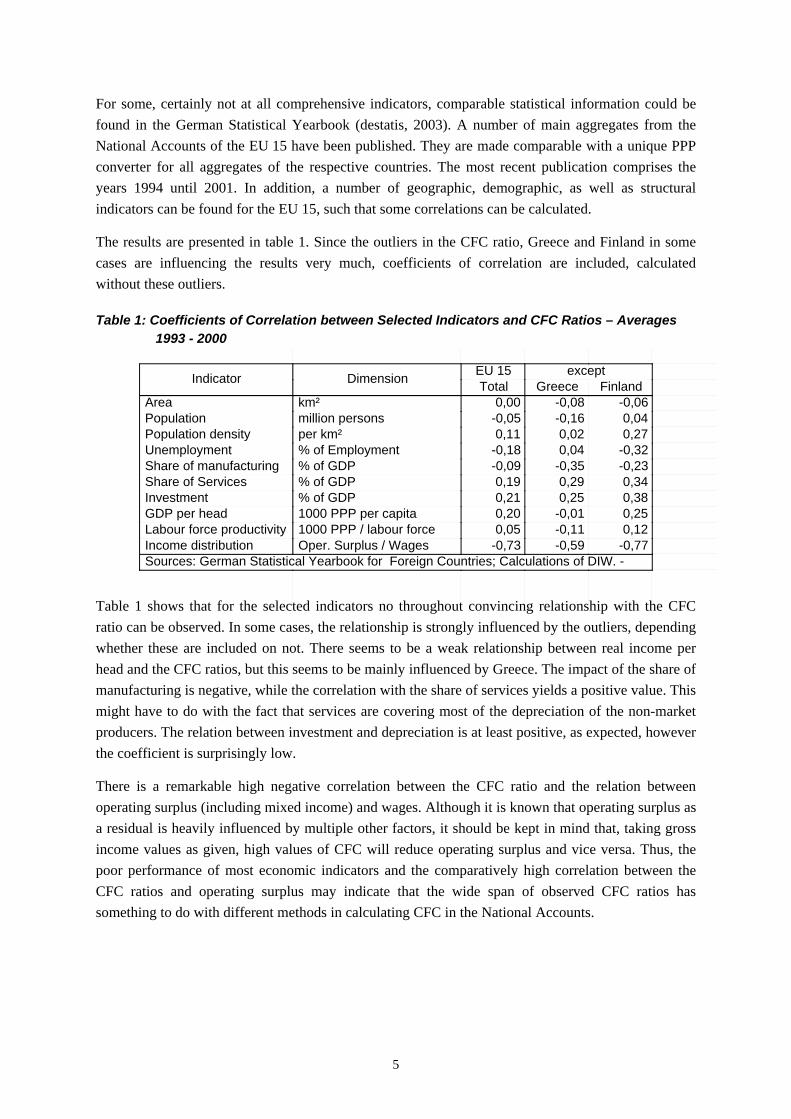
For some, certainly not at all comprehensive indicators, comparable statistical information could be found in the German Statistical Yearbook (destatis, 2003). A number of main aggregates from the National Accounts of the EU 15 have been published. They are made comparable with a unique PPP converter for all aggregates of the respective countries. The most recent publication comprises the years 1994 until 2001. In addition, a number of geographic, demographic, as well as structural indicators can be found for the EU 15, such that some correlations can be calculated.

The results are presented in table 1. Since the outliers in the CFC ratio, Greece and Finland in some cases are influencing the results very much, coefficients of correlation are included, calculated without these outliers.

Table 1: Coefficients of Correlation between Selected Indicators and CFC Ratios – Averages 1993 - 2000

Table 1 shows that for the selected indicators no throughout convincing relationship with the CFC ratio can be observed. In some cases, the relationship is strongly influenced by the outliers, depending whether these are included on not. There seems to be a weak relationship between real income per head and the CFC ratios, but this seems to be mainly influenced by Greece. The impact of the share of manufacturing is negative, while the correlation with the share of services yields a positive value. This might have to do with the fact that services are covering most of the depreciation of the non-market producers. The relation between investment and depreciation is at least positive, as expected, however the coefficient is surprisingly low.

There is a remarkable high negative correlation between the CFC ratio and the relation between operating surplus (including mixed income) and wages. Although it is known that operating surplus as a residual is heavily influenced by multiple other factors, it should be kept in mind that, taking gross income values as given, high values of CFC will reduce operating surplus and vice versa. Thus, the poor performance of most economic indicators and the comparatively high correlation between the CFC ratios and operating surplus may indicate that the wide span of observed CFC ratios has something to do with different methods in calculating CFC in the National Accounts.

DimensionIndicator

Sources: German Statistical Yearbook for Foreign Countries; Calculations of DIW. -

except EU 15FinlandGreeceTotal

-0,06-0,080,00km²Area0,04-0,16-0,05million personsPopulation0,270,020,11per km²Population density

-0,320,04-0,18% of EmploymentUnemployment-0,23-0,35-0,09% of GDPShare of manufacturing0,340,290,19% of GDPShare of Services0,380,250,21% of GDPInvestment0,25-0,010,201000 PPP per capitaGDP per head0,12-0,110,051000 PPP / labour forceLabour force productivity

-0,77-0,59-0,73Oper. Surplus / WagesIncome distribution

6

3 The Political Dimension Before the subject of known methodological differences between CFC estimates in EU countries is approached, a remark on the political aspects of CFC calculations should be made. CFC is not only an important variable for productivity analysis; it also has a direct impact on relevant political decisions. CFC is an important variable not only in productivity analysis; it also has a direct impact on relevant political decisions. CFC is a component in calculating value added for the institutional sector of general government and for dwellings. Up to one third of total CFC can be attributed to these activities. Differences between countries in the methodologies used for measuring CFC therefore might have a direct influence on the level of GDP and in a number of important EU contexts, such as:

o Contributions for the Community budget, o Assessment of the deficit criteria for public budgets.

It is not known to what extent differences in CFC ratios have to be attributed to such methodological differences, neither is it known to what extent value added and GDP are influenced by the differences. However, it might be interesting to get an idea of the magnitude, such differences can result in.

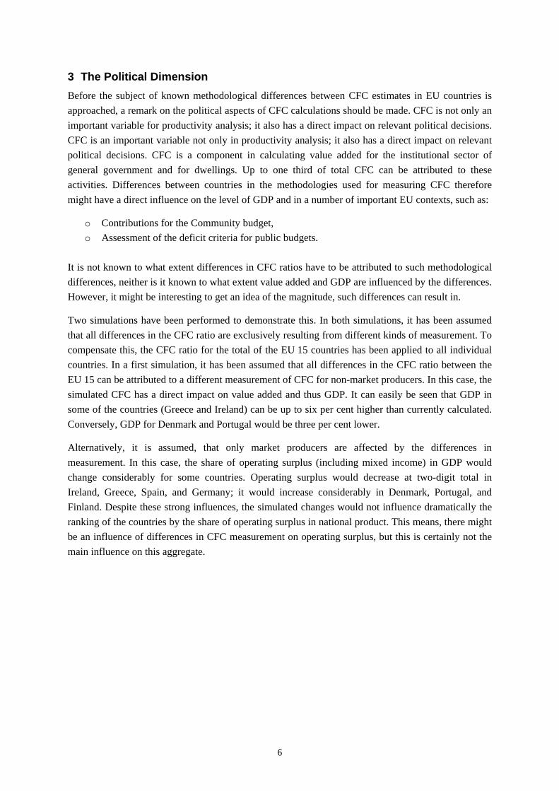
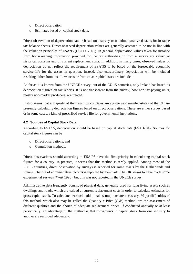
Two simulations have been performed to demonstrate this. In both simulations, it has been assumed that all differences in the CFC ratio are exclusively resulting from different kinds of measurement. To compensate this, the CFC ratio for the total of the EU 15 countries has been applied to all individual countries. In a first simulation, it has been assumed that all differences in the CFC ratio between the EU 15 can be attributed to a different measurement of CFC for non-market producers. In this case, the simulated CFC has a direct impact on value added and thus GDP. It can easily be seen that GDP in some of the countries (Greece and Ireland) can be up to six per cent higher than currently calculated. Conversely, GDP for Denmark and Portugal would be three per cent lower.

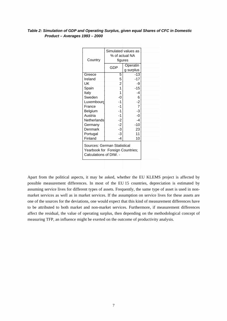
Alternatively, it is assumed, that only market producers are affected by the differences in measurement. In this case, the share of operating surplus (including mixed income) in GDP would change considerably for some countries. Operating surplus would decrease at two-digit total in Ireland, Greece, Spain, and Germany; it would increase considerably in Denmark, Portugal, and Finland. Despite these strong influences, the simulated changes would not influence dramatically the ranking of the countries by the share of operating surplus in national product. This means, there might be an influence of differences in CFC measurement on operating surplus, but this is certainly not the main influence on this aggregate.

7

Table 2: Simulation of GDP and Operating Surplus, given equal Shares of CFC in Domestic Product – Averages 1993 – 2000

Apart from the political aspects, it may be asked, whether the EU KLEMS project is affected by possible measurement differences. In most of the EU 15 countries, depreciation is estimated by assuming service lives for different types of assets. Frequently, the same type of asset is used in non-market services as well as in market services. If the assumption on service lives for these assets are one of the sources for the deviations, one would expect that this kind of measurement differences have to be attributed to both market and non-market services. Furthermore, if measurement differences affect the residual, the value of operating surplus, then depending on the methodological concept of measuring TFP, an influence might be exerted on the outcome of productivity analysis.

figures% of actual NA

Simulated values as

Country

g surplusOperatinGDP

Calculations of DIW. -Yearbook for Foreign Countries;Sources: German Statistical

-135Greece-175Ireland-92UK

-151Spain-41Italy6-0Sweden

-2-1Luxembourg7-1France

-3-1Belgium-0-1Austria-4-2Netherlands

-10-2Germany23-3Denmark11-3Portugal10-4Finland

8

Figure 2: Share of Operating Surplus in Net Domestic Product – Original and Simulated – Averages 1993 – 2000

0 10 20 30 40 50 60 Share of Operating Surplus in NDP %

GreeceIreland

UKSpain

ItalySweden

LuxembourgFrance

BelgiumAustria

NetherlandsGermanyDenmarkPortugalFinland

Simulated Shares

NationalAccounts

9

4 Methodological Differences in Calculating CFC Apart from pure measurement errors, an assessment of the differences in the depreciation ratio may be improved by analysing the different methods applied in the EU countries to estimate CFC. Frequently, measurement errors have to do with insufficient coverage of the economy. Equally, the choice of the applied method to measure CFC in many cases has the origin in insufficient coverage. The following section is based mainly on the results of an UNECE survey on this subject addressed to the National Statistical Offices of the UN members. The survey was conducted in 2003 and published in 2004 (UNECE, 2004). The responses by the National Statistical Offices to the questionnaire are very heterogeneous. It has been attempted to make them comparable in a systematic way. However, it is possible that some of the descriptions in this paper might not fully reflect the intentions of the respondents.

According to the survey, methods applied for calculating CFC in EU member states vary considerably. It has been tried to compare these different methods by separating individual components of the method applied. However, it has to be taken into account that some of these components may depend on each other, such that it will not be easy to explain differences in depreciation ratios as a result of one of the discussed components alone.

The following aspects of the UNECE survey will be discussed.

Sources:

o Depreciation o Capital-Stock o Service Lives

Breakdown in service life estimates:

o Assets o Industries

Model applied for capital stock estimates:

o Discard Function o BEA model o BFA model

Depreciation schedules:

o Linear o Geometric

4.1 Sources of Depreciation Data

One of the most important factors, which might influence the outcome are the sources applied. In the case of depreciation, two main sources have been reported:

10

o Direct observation, o Estimates based on capital stock data.

Direct observation of depreciation can be based on a survey or on administrative data, as for instance tax balance sheets. Direct observed depreciation values are generally assessed to be not in line with the valuation principles of ESA'95 (OECD, 2001). In general, depreciation values taken for instance from book-keeping information provided for the tax authorities or from a survey are valued at historical costs instead of current replacement costs. In addition, in many cases, observed values of depreciation do not reflect the requirement of ESA’95 to be based on the foreseeable economic service life for the assets in question. Instead, also extraordinary depreciation will be included resulting either from tax allowances or from catastrophic losses are included.

As far as it is known from the UNECE survey, out of the EU 15 countries, only Ireland has based its depreciation figures on tax reports. It is not transparent from the survey, how non tax-paying units, mostly non-market producers, are treated.

It also seems that a majority of the transition countries among the new member-states of the EU are presently calculating depreciation figures based on direct observations. These are either survey based or in some cases, a kind of prescribed service life for governmental institutions.

4.2 Sources of Capital Stock Data

According to ESA'95, depreciation should be based on capital stock data (ESA 6.04). Sources for capital stock figures can be

o Direct observations, and o Cumulation methods.

Direct observations should according to ESA’95 have the first priority in calculating capital stock figures for a country. In practice, it seems that this method is rarely applied. Among most of the EU 15 countries, direct observation by surveys is reported for some assets by the Netherlands and France. The use of administrative records is reported by Denmark. The UK seems to have made some experimental surveys (West 1998), but this was not reported in the UNECE survey.

Administrative data frequently consist of physical data, generally used for long living assets such as dwellings and roads, which are valued at current replacement costs in order to calculate estimates for gross capital stock. To calculate net stock, additional assumptions are necessary. Major difficulties of this method, which also may be called the Quantity x Price (QxP) method, are the assessment of different qualities and the choice of adequate replacement prices. If conducted annually or at least periodically, an advantage of the method is that movements in capital stock from one industry to another are recorded adequately.

11

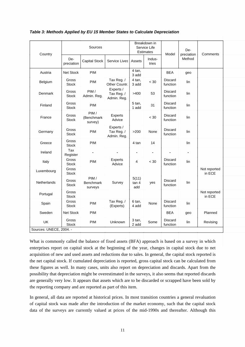
Table 3: Methods Applied by EU 15 Member States to Calculate Depreciation

What is commonly called the balance of fixed assets (BFA) approach is based on a survey in which enterprises report on capital stock at the beginning of the year, changes in capital stock due to net acquisition of new and used assets and reductions due to sales. In general, the capital stock reported is the net capital stock. If cumulated depreciation is reported, gross capital stock can be calculated from these figures as well. In many cases, units also report on depreciation and discards. Apart from the possibility that depreciation might be overestimated in the surveys, it also seems that reported discards are generally very low. It appears that assets which are to be discarded or scrapped have been sold by the reporting company and are reported as part of this item.

In general, all data are reported at historical prices. In most transition countries a general revaluation of capital stock was made after the introduction of the market economy, such that the capital stock data of the surveys are currently valued at prices of the mid-1990s and thereafter. Although this

CommentsMethod

preciationDe-

ModelCountry

Sources: UNECE, 2004. -

EstimatesService Life

Breakdown inSources

triesIndus-AssetsService LivesCapital Stock

preciationDe-

geoBEA3 add4 tan,PIMNet StockAustria

linfunctionDiscard< 30

3 add4 tan,

Other Countr.Tax Reg. /PIM

StockGrossBelgium

linfunctionDiscard53>400

Admin. Reg.Tax Reg. /Experts /

Admin. Reg.PIM /

StockGrossDenmark

linfunctionDiscard31

1 add5 tan,PIM

StockGrossFinland


AdviceExperts

survey)(Benchmark

PIM /

StockGrossFrance

linfunctionDiscardNone>200

Admin. Reg.Tax Reg. /Experts /

PIMStockGrossGermany

lin144 tanPIMStockGrossGreece

------RegisterTaxIreland


AdviceExpertsPIM

StockGrossItaly

in ECENot reported

StockGrossLuxembourg

linfunctionDiscardyes

addtan 45(11)

Surveysurveys

BenchmarkPIM /

StockGrossNetherlands

in ECENot reported

StockGrossPortugal

linfunctionDiscardNone

4 add6 tan,

(Experts)Tax Reg. /PIM

StockGrossSpain

PlannedgeoBEAPIMNet StockSweden

RevisinglinfunctionDiscardSome

2 add3 tan,UnknownPIM

StockGrossUK

12

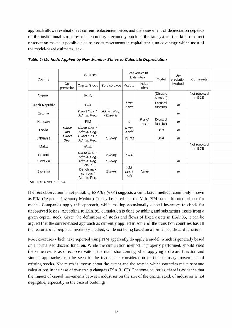
approach allows revaluation at current replacement prices and the assessment of depreciation depends on the institutional structures of the country’s economy, such as the tax system, this kind of direct observation makes it possible also to assess movements in capital stock, an advantage which most of the model-based estimates lack.

Table 4: Methods Applied by New Member States to Calculate Depreciation

If direct observation is not possible, ESA’95 (6.04) suggests a cumulation method, commonly known as PIM (Perpetual Inventory Method). It may be noted that the M in PIM stands for method, not for model. Companies apply this approach, while making occasionally a total inventory to check for unobserved losses. According to ESA’95, cumulation is done by adding and subtracting assets from a given capital stock. Given the definitions of stocks and flows of fixed assets in ESA’95, it can be argued that the survey-based approach as currently applied in some of the transition countries has all the features of a perpetual inventory method, while not being based on a formalised discard function.

Most countries which have reported using PIM apparently do apply a model, which is generally based on a formalised discard function. While the cumulation method, if properly performed, should yield the same results as direct observation, the main shortcoming when applying a discard function and similar approaches can be seen in the inadequate consideration of inter-industry movements of existing stocks. Not much is known about the extent and the way in which countries make separate calculations in the case of ownership changes (ESA 3.103). For some countries, there is evidence that the impact of capital movements between industries on the size of the capital stock of industries is not negligible, especially in the case of buildings.

CommentsMethod

preciationDe-

ModelCountry

Sources: UNECE, 2004.

EstimatesBreakdown inSources

triesIndus-AssetsService LivesCapital Stock

preciationDe-

in ECENot reported

function)(Discard(PIM)Cyprus

linfunctionDiscard

2 add4 tan,PIMCzech Republic

lin/ ExpertsAdmin. Reg.

Admin. Reg.Direct Obs. /Estonia

linfunctionDiscard

more9 and4PIMHungary

linBFA4 add5 tan,

Admin. Reg.Direct Obs. /

Obs.DirectLatvia

linBFA21 tanSurveyAdmin. Reg.Direct Obs. /

Obs.DirectLithuania

in ECENot reported(PIM)Malta

8 tanSurveyAdmin. Reg.Direct Obs. /Poland

linSurveyAdmin. Reg.Slovakia

linNoneadd

tan, 3>12

Survey

Admin. Reg.surveys /

BenchmarkPIM /

Slovenia

13

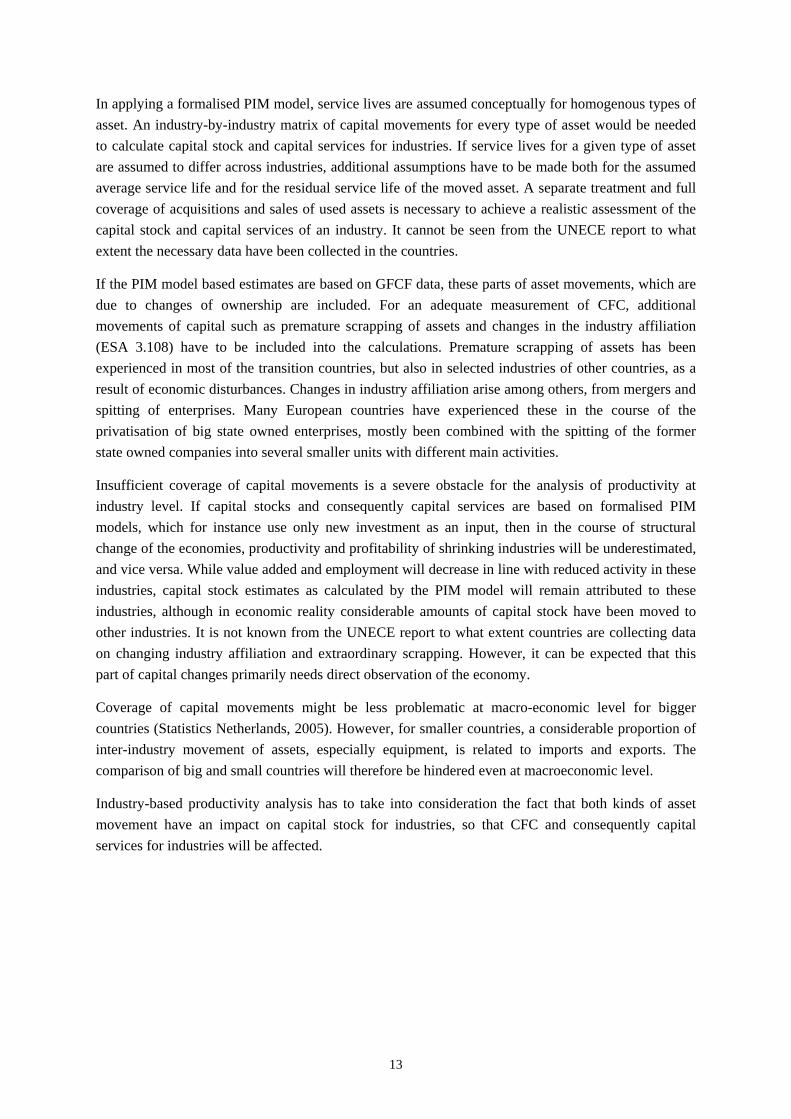
In applying a formalised PIM model, service lives are assumed conceptually for homogenous types of asset. An industry-by-industry matrix of capital movements for every type of asset would be needed to calculate capital stock and capital services for industries. If service lives for a given type of asset are assumed to differ across industries, additional assumptions have to be made both for the assumed average service life and for the residual service life of the moved asset. A separate treatment and full coverage of acquisitions and sales of used assets is necessary to achieve a realistic assessment of the capital stock and capital services of an industry. It cannot be seen from the UNECE report to what extent the necessary data have been collected in the countries.

If the PIM model based estimates are based on GFCF data, these parts of asset movements, which are due to changes of ownership are included. For an adequate measurement of CFC, additional movements of capital such as premature scrapping of assets and changes in the industry affiliation (ESA 3.108) have to be included into the calculations. Premature scrapping of assets has been experienced in most of the transition countries, but also in selected industries of other countries, as a result of economic disturbances. Changes in industry affiliation arise among others, from mergers and spitting of enterprises. Many European countries have experienced these in the course of the privatisation of big state owned enterprises, mostly been combined with the spitting of the former state owned companies into several smaller units with different main activities.

Insufficient coverage of capital movements is a severe obstacle for the analysis of productivity at industry level. If capital stocks and consequently capital services are based on formalised PIM models, which for instance use only new investment as an input, then in the course of structural change of the economies, productivity and profitability of shrinking industries will be underestimated, and vice versa. While value added and employment will decrease in line with reduced activity in these industries, capital stock estimates as calculated by the PIM model will remain attributed to these industries, although in economic reality considerable amounts of capital stock have been moved to other industries. It is not known from the UNECE report to what extent countries are collecting data on changing industry affiliation and extraordinary scrapping. However, it can be expected that this part of capital changes primarily needs direct observation of the economy.

Coverage of capital movements might be less problematic at macro-economic level for bigger countries (Statistics Netherlands, 2005). However, for smaller countries, a considerable proportion of inter-industry movement of assets, especially equipment, is related to imports and exports. The comparison of big and small countries will therefore be hindered even at macroeconomic level.

Industry-based productivity analysis has to take into consideration the fact that both kinds of asset movement have an impact on capital stock for industries, so that CFC and consequently capital services for industries will be affected.

14

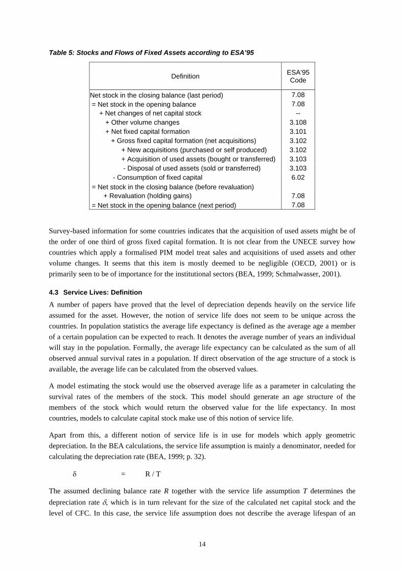
Table 5: Stocks and Flows of Fixed Assets according to ESA’95

Definition ESA’95 Code

Net stock in the closing balance (last period) 7.08 = Net stock in the opening balance 7.08

+ Net changes of net capital stock -- + Other volume changes 3.108 + Net fixed capital formation 3.101 + Gross fixed capital formation (net acquisitions) 3.102

+ New acquisitions (purchased or self produced) 3.102 + Acquisition of used assets (bought or transferred) 3.103 - Disposal of used assets (sold or transferred) 3.103

- Consumption of fixed capital 6.02 = Net stock in the closing balance (before revaluation)

+ Revaluation (holding gains) 7.08 = Net stock in the opening balance (next period) 7.08

Survey-based information for some countries indicates that the acquisition of used assets might be of the order of one third of gross fixed capital formation. It is not clear from the UNECE survey how countries which apply a formalised PIM model treat sales and acquisitions of used assets and other volume changes. It seems that this item is mostly deemed to be negligible (OECD, 2001) or is primarily seen to be of importance for the institutional sectors (BEA, 1999; Schmalwasser, 2001).

4.3 Service Lives: Definition

A number of papers have proved that the level of depreciation depends heavily on the service life assumed for the asset. However, the notion of service life does not seem to be unique across the countries. In population statistics the average life expectancy is defined as the average age a member of a certain population can be expected to reach. It denotes the average number of years an individual will stay in the population. Formally, the average life expectancy can be calculated as the sum of all observed annual survival rates in a population. If direct observation of the age structure of a stock is available, the average life can be calculated from the observed values.

A model estimating the stock would use the observed average life as a parameter in calculating the survival rates of the members of the stock. This model should generate an age structure of the members of the stock which would return the observed value for the life expectancy. In most countries, models to calculate capital stock make use of this notion of service life.

Apart from this, a different notion of service life is in use for models which apply geometric depreciation. In the BEA calculations, the service life assumption is mainly a denominator, needed for calculating the depreciation rate (BEA, 1999; p. 32).

δ = R / T

The assumed declining balance rate R together with the service life assumption T determines the depreciation rate δ, which is in turn relevant for the size of the calculated net capital stock and the level of CFC. In this case, the service life assumption does not describe the average lifespan of an

15

asset in the net capital stock. The service life assumption applied in a geometric depreciation formula defined in this way is not necessarily comparable with the notion of average service life in the sense of average life expectancy2.

In commercial uses of geometric depreciation, the declining-balance rate frequently is assumed to be 2. This is for instance the standard value, which is used in spreadsheet applications like MS Excel. The US Bureau for Economic Analysis (BEA), which applies geometric depreciation, assumes in most cases a factor of 1.65. For some assets, as for instance CT equipment, the value of the declining balance rate goes up to a value of more than two. In other cases, it is around 0.9, as in the case of dwellings and other kinds of buildings (BEA 1999, p. 29).

4.4 Service Lives: Sources

A variety of different sources for service lives has been reported. Most countries use several sources. These are experts’ advises for instance in the case of Spain, Italy, France, Germany, and Estonia. Information from the tax register is used by Spain, Germany, Belgium, and a. o. Some countries use the results of other countries estimates, especially the US estimates. Frequently, use is made of administrative data (Germany, Denmark, Estonia, a. o.). Some countries also have surveys on service lives, as for instance the Netherlands, Finland, and some of the transition countries.

It is not always clear, what the surveys on service lives actually are reporting. In some surveys, reporting units are asked for the assumed service life, the actual service life and expected service life. In any case, a survey asking directly for the service life needs a very detailed asset breakdown. Otherwise, the reporting units would have to apply a weighting method for averaging the service lives of the assets in use. To cover homogeneous assets, the necessary breakdown would have to be considerably deeper then the AN classification suggested by ESA'95 (table 7.1) for gross fixed capital formation (GFCF) or the one in the delivery programme of Eurostat

Known surveys of asset service lives (Cope, 1998) ask for data on more than two hundred different types of assets. The asset breakdown in the BEA estimates is about 150. For the German calculations, Destatis (Schmalwasser, 2001) uses more than 200 different types of assets. An idea of the magnitude of different service lives applied by firms might also be given by the fact that the German tables for tax service lives cover more than 2 000 different types of assets (BMF: AfA-Tabellen).

Another method of obtaining information on service lives is to ask for the age structure of the stock, preferably the gross stock (e.g. Czech Republic, Lithuania, Netherlands). In this case, values which are available in the companies’ accounting system can be aggregated and reported. Since values are normally reported at historic acquisition prices, additional assumptions and a revaluation at current replacement costs will be needed.

4.5 Service Lives: Degree of Differentiation

Although it is known (OECD, 2001) and easy to demonstrate that service life assumptions have a strong influence on capital stock and consumption of fixed capital, it is difficult, to measure its impact

2 In fact, if geometric depreciation is assumed together with an infinite serving period, the average life expectancy M of an asset in net capital stock converges with an increasing serving period to the reciprocal of the depreciation rate. This can easily be calculated with the sum formula for geometric rows.

16

on the published data of consumption of fixed capital for the countries in question. Main reason for this is that no comparable breakdowns of assets are made for the service life assumptions. Breakdown in the context of service life does not mean the asset and industry breakdown for which GFCF time series are available. This information has been provided for the countries in the EU KLEMS questionnaire. For an assessment of the assumptions on service lives however, it is necessary to know, for how many types of assets, different service life assumptions have been applied. There may be an A 60 industry breakdown and an asset breakdown of the same order available. If only a unique service life assumption have been applied, this would result with respect to depreciation in the same value as if the exercise had been done for the aggregated time-series.

ESA'95 does not give a specific suggestion on the necessary degree of asset breakdown. ESA'95 suggests that the average service life of a specific asset should be the regular case for all units of the economy (ESA’95, 6.04). The underlying idea is that there exists some kind of homogeneous type of capital asset, which experiences economic obsolescence. Clearly, in this concept the service life has to be seen as an economic variable. The underlying idea of a unique service life for homogeneous types of asset is the model of perfect competition. However, from the economic point of view, the asset breakdown in the AN classification for GFCF (ESA'95, 3.106) certainly cannot be seen to be of sufficient detail to represent homogeneous types of asset.

Whether the implicit economic model is a realistic representation of existing economies, might be another question, yet in practice, only a few countries seem to adhere to the concept of a unique service live by types of asset. According to the UNECE survey in most EU 15 countries, the asset breakdown is reported to be more or less in line or below that of the AN classification as given in ESA'95. Only Denmark and Germany are reporting an asset breakdown, which might be differentiated enough to cover individual assets, which might be assumed to represent homogeneous types of asset. Yet, Denmark is reporting to have an additional breakdown according to the industries in which the assets are used.

Reasons for an additional industry breakdown can be twofold:

a) The applied asset classification is not deep enough to cover homogeneous types of asset, or b) Different market structures in the industries will induce different economic service lives for the same type of asset.

An additional industry breakdown seems to be applied in many countries. In the EU KLEMS questionnaire, some consortium members have reported a very detailed breakdown of GFCF by industry and type of asset (EU KLEMS, 2005). Not necessarily, these industry breakdowns are made with respect to different service life assumptions. In these countries, where according to the UNECE report, information on service lives has been reported by type of asset and by industry (e. g. Belgium, France, Italy), it becomes transparent, that with some exceptions, the degree of service life differentiation between industries seems not to be very high.

4.6 Service Lives: Comparisons

A varying degree of breakdown by asset and by industry makes it difficult to compare the assumed service lives across countries. In some cases, it might be possible to compare the assumptions for a specified asset for two selected countries. However, to arrive at an assessment of the impact of service

17

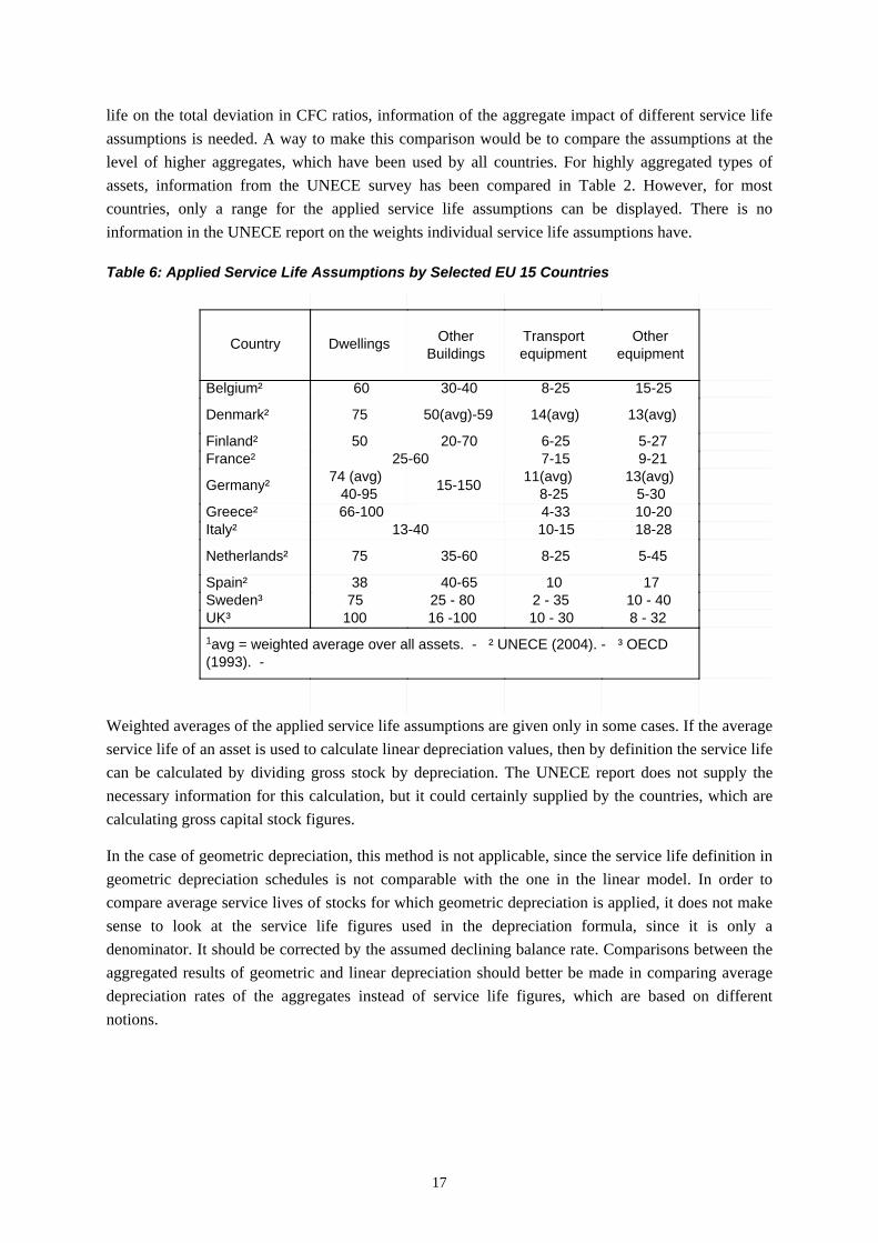
life on the total deviation in CFC ratios, information of the aggregate impact of different service life assumptions is needed. A way to make this comparison would be to compare the assumptions at the level of higher aggregates, which have been used by all countries. For highly aggregated types of assets, information from the UNECE survey has been compared in Table 2. However, for most countries, only a range for the applied service life assumptions can be displayed. There is no information in the UNECE report on the weights individual service life assumptions have.

Table 6: Applied Service Life Assumptions by Selected EU 15 Countries

Weighted averages of the applied service life assumptions are given only in some cases. If the average service life of an asset is used to calculate linear depreciation values, then by definition the service life can be calculated by dividing gross stock by depreciation. The UNECE report does not supply the necessary information for this calculation, but it could certainly supplied by the countries, which are calculating gross capital stock figures.

In the case of geometric depreciation, this method is not applicable, since the service life definition in geometric depreciation schedules is not comparable with the one in the linear model. In order to compare average service lives of stocks for which geometric depreciation is applied, it does not make sense to look at the service life figures used in the depreciation formula, since it is only a denominator. It should be corrected by the assumed declining balance rate. Comparisons between the aggregated results of geometric and linear depreciation should better be made in comparing average depreciation rates of the aggregates instead of service life figures, which are based on different notions.

25-60

13-40

(1993). - 1avg = weighted average over all assets. - ² UNECE (2004). - ³ OECD

equipmentOther

equipmentTransport

BuildingsOtherDwellingsCountry

15-258-2530-40 60Belgium²

13(avg)14(avg)50(avg)-5975Denmark²

5-276-2520-7050Finland² 9-217-15France²

5-30 13(avg)

8-2511(avg) 15-15040-95

74 (avg) Germany²

10-204-33 66-100Greece² 18-2810-15Italy²

5-45 8-25 35-6075Netherlands²

171040-6538Spain² 10 - 40 2 - 35 25 - 80 75 Sweden³ 8 - 32 10 - 30 16 -100 100 UK³

18

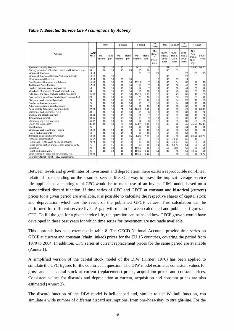
Table 7: Selected Service Life Assumptions by Activity

Between levels and growth rates of investment and depreciation, there exists a reproducible non-linear relationship, depending on the assumed service life. One way to assess the implicit average service life applied in calculating total CFC would be to make use of an inverse PIM model, based on a standardised discard function. If time series of CFC and GFCF at constant and historical (current) prices for a given period are available, it is possible to calculate the respective shares of capital stock and depreciation which are the result of the published GFCF values. This calculation can be performed for different service lives. A gap will remain between calculated and published figures of CFC. To fill the gap for a given service life, the question can be asked how GFCF growth would have developed in these past years for which time series for investment are not made available.

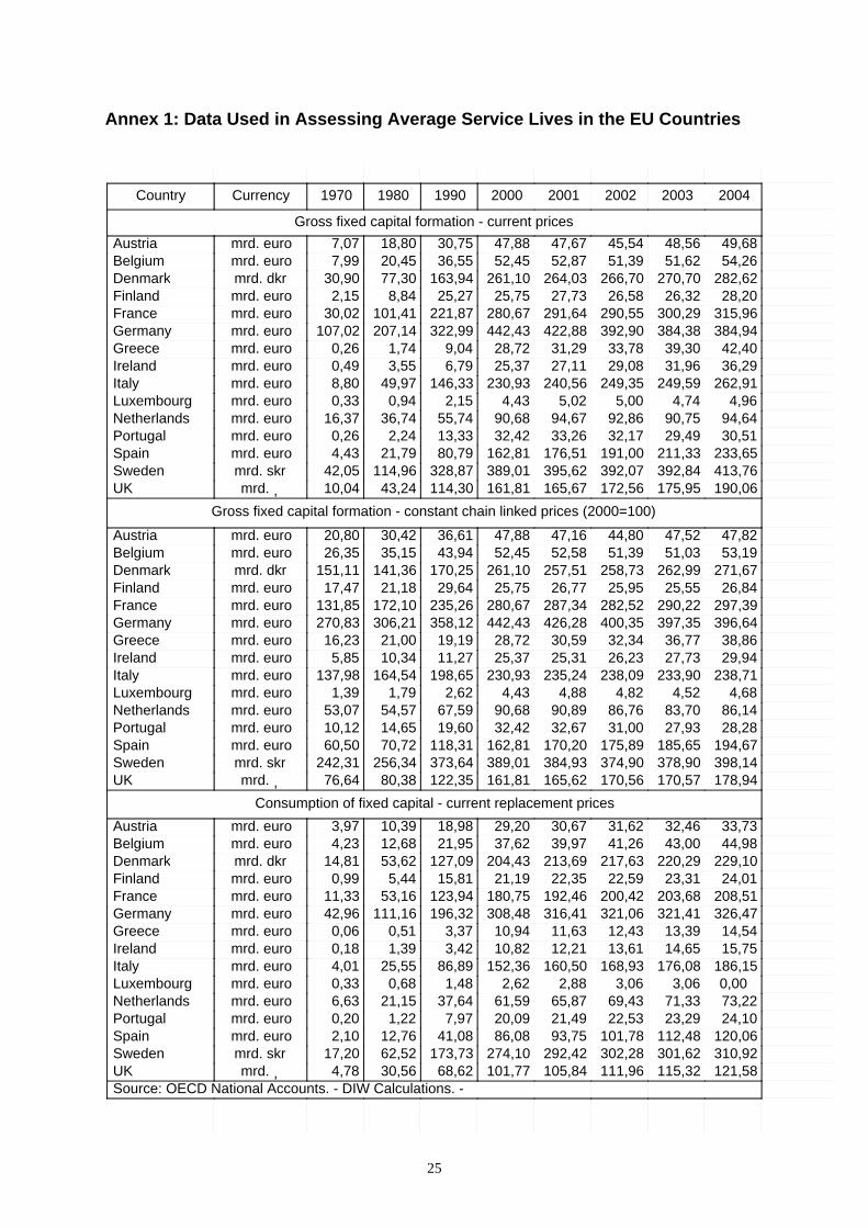
This approach has been exercised in table 8. The OECD National Accounts provide time series on GFCF at current and constant (chain linked) prices for the EU 15 countries, covering the period from 1970 to 2004. In addition, CFC series at current replacement prices for the same period are available (Annex 1).

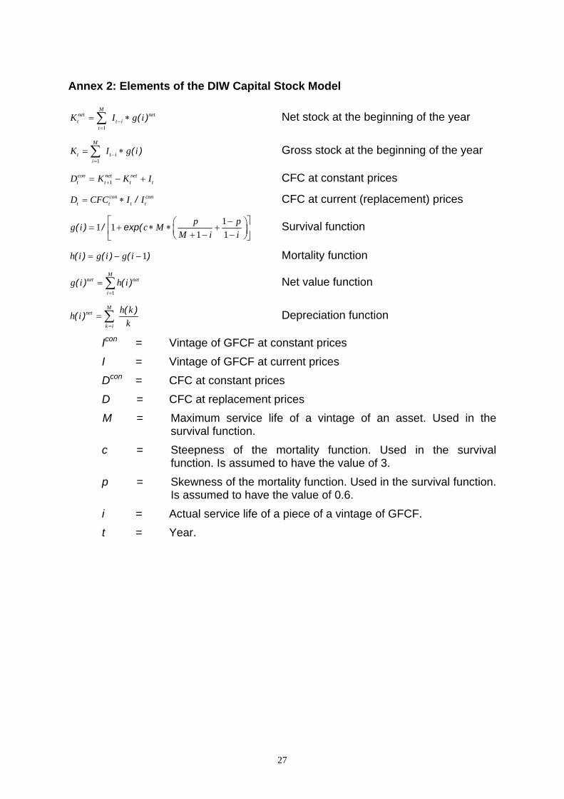
A simplified version of the capital stock model of the DIW (Kirner, 1970) has been applied to simulate the CFC figures for the countries in question. The DIW model estimates consistent values for gross and net capital stock at current (replacement) prices, acquisition prices and constant prices. Consistent values for discards and depreciation at current, acquisition and constant prices are also estimated (Annex 2).

The discard function of the DIW model is bell-shaped and, similar to the Weibull function, can simulate a wide number of different discard assumptions, from one-hoss-shay to straight-line. For the

rev 1NACEActivities

Sources: UNECE, 2004. - DIW Calculations. -

FinlandmanyGer-BelgiumItaly

manyGer-FinlandBelgiumItaly

turesStruc-

ingsBuild-

dentialResi-Non

turesStruc-ings &Build-



mentEquip-

&chinery

Ma-

portTrans-

chineryMa-

portTrans-

chineryMa-

portTrans-

chineryMa-

30-5035-403751095-121215101801-02Agriculture, Hunting, Forestry 3935010152515101805Fishing; operation of fish hatcheries and fish farms; etc

2530232171810-14Mining and Quarrying2335101810-12Mining and Quarrying of Energy Producing Materials14333581020101813-14Other Mining and Quarrying

254033343514717-191020101815-16Food Products, Beverages and Tobacco4035403835147141019101817-18Textiles and Textile Products4035413835147141018101819Leather; manufacture of luggage,etc.25353545351110161018101820Wood and of products of wood and cork, etc.3540354535126-1015-181019101821-22Pulp, paper and paper products, publishing, printing40352738351810231018101823Coke, refined petroleum products and nuclear fuel35402734351510181018101824Chemicals and chemical products4045343435137181017101825Rubber and plastic products40403030351410191019101826Other non-metallic mineral products

30-4040293535148-1216-231021101827-28Basic metals, fabricated metal products3040303535138131019101829Machinery and equipment n.e.c. 3040313535127111019101830-33Electrical and optical equipment4045303535119151018101834-35Transport equipment3535383535128141018101836-37Manufacturing n.e.c; recycling

35-4045-50454240198-1024-271025101840-41Energy and water supply 3040414291010102045Construction 3040504065101015815101850-52Wholesale and retail trade; repairs

40594065121015815101855Hotels and restaurants 20-70 20-50334080137-255-251515101860-64Transport, storage and communication

4066 40-60651010815101865-67Financial intermediation705066 40-6080101015815101870-74Real estate, renting and business activities705051 60-7080111015815152875Public administration and defence; social security705059 (60)5781010-15815101880Education 7040-50584035118-1010-15815101885Health and social work

40-7050484088-1010-1581590-93Other community, social and personal services

19

simulations, it has been assumed that the aggregated discard function for the total economy in the countries is left steep3. In the UNECE survey, a number of countries have reported to apply changing service live assumptions. The reason for this is that either by economic and technological influences service live has changed. In the aggregate, the average service life can also change due to structural changes. The focus of this exercise is not to estimate capital stock and CFC in the respective countries. Instead, the aim is to evaluate the rough magnitude of the implicit average service live assumption used in calculating CFC. In the simulation procedure therefore, a constant service life has been applied for all years. Linear depreciation and no age efficiency profile are assumed. GFCF values are treated like new investment. Revaluation of CFC at constant prices is done with the average price indices for total GFCF.

Based on this model for every country the necessary time path for GFCF before 1970 can be calculated, given alternative service lives. It can be seen that, in general, the higher the service life assumption, the lower will be the resulting GFCF path before 1970. For some service lives, no realistic GFCF paths before 1970 could be found. This means that GFCF growth rates above 25 per cent would be needed to simulate the given CFC values. Growth rates of this dimension can also be a sign that the initial capital stock has been assumed to be very small. This may be the case in countries which experienced a rapid growth in GFCF in the observed period. In addition, it should not be forgotten that during the observation period CFC values in some years increased greatly due to inflation.

Although in most of the countries the period before 1970 was one of high capital accumulation, it should be noted that the calculated GFCF path is not comparable with possibly existing investment figures from other sources for this period. The calculated figures can only represent this changing part of the unknown GFCF values for the years before 1970 which is relevant for the CFC values in the period thereafter. With an increasing backward distance from 1970, the weight of assets with a high service life increases, while assets with a low service life which have been part of GFCF in these years are not relevant for the period following 1970. Therefore, if the observed relationship between GFCF and CFC produces a very low service life the impact of pre-1970 GFCF values becomes very small.

Clearly, the calculated path of GFCF is also influenced by the divergence of the normalised model applied from the factual model in use for the respective countries. However, the general structure of the results will not be very different if major features of the model are changed, for instance by applying geometric instead of linear depreciation. The procedure described can be abbreviated by asking for the combination of service life assumption and GFCF growth in the past, which will give the best adaptation to the published time series of CFC. This non-linear problem can be solved by applying OLS to observed and simulated values in the framework of a Newton optimising procedure.

3 This is based on the idea that every aggregated function can be seen as the result of several discard function with different average service lives. In this case, the aggregate of these discard function will always result in a left steep discard function for the total. In practice, a multitude of papers have demonstrated that, compared with service live assumptions, differences in the shape of the discard function are of minor influence on the CFC estimates.

20

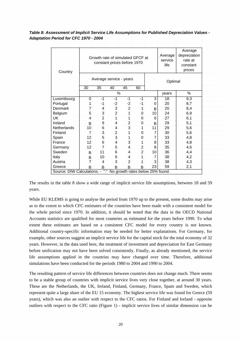
Table 8: Assessment of Implicit Service Life Assumptions for Published Depreciation Values - Adaptation Period for CFC 1970 - 2004

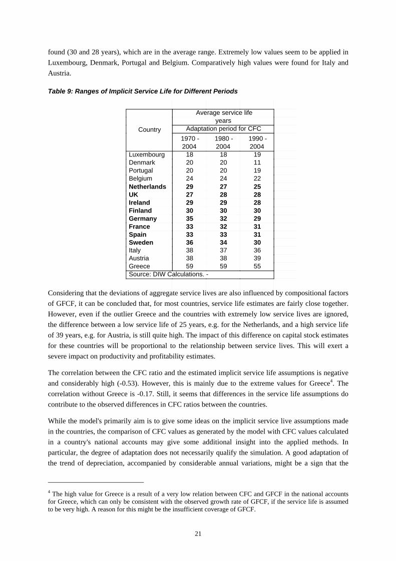
The results in the table 8 show a wide range of implicit service life assumptions, between 18 and 59 years.

While EU KLEMS is going to analyse the period from 1970 up to the present, some doubts may arise as to the extent to which CFC estimates of the countries have been made with a consistent model for the whole period since 1970. In addition, it should be noted that the data in the OECD National Accounts statistics are qualified for most countries as estimated for the years before 1990. To what extent these estimates are based on a consistent CFC model for every country is not known. Additional country-specific information may be needed for better explanations. For Germany, for example, other sources suggest an implicit service life for the capital stock for the total economy of 32 years. However, in the data used here, the treatment of investment and depreciation for East Germany before unification may not have been solved consistently. Finally, as already mentioned, the service life assumptions applied in the countries may have changed over time. Therefore, additional simulations have been conducted for the periods 1980 to 2004 and 1990 to 2004.

The resulting pattern of service life differences between countries does not change much. There seems to be a stable group of countries with implicit service lives very close together, at around 30 years. These are the Netherlands, the UK, Ireland, Finland, Germany, France, Spain and Sweden, which represent quite a large share of the EU 15 economy. The highest service life was found for Greece (59 years), which was also an outlier with respect to the CFC ratios. For Finland and Ireland - opposite outliers with respect to the CFC ratio (Figure 1) - implicit service lives of similar dimension can be

Country

Optimal

Source: DIW Calculations. - "." No growth rates below 25% found.

pricesconstantrate at

depreciationAverage

lifeserviceAverage

constant prices before 1970Growth rate of simulated GFCF at

Average service - years

6045403530%years%9,3183-1-1-1-10Luxembourg8,7200-1-2-2-11Portugal8,420B12347Denmark6,9241001235Belgium6,127601124UK5,129B0249BIreland5,62911134610Netherlands5,630701237Finland4,8337013512Spain4,8338134612France4,6358245712Germany4,4361024611BSweden4,238714610BItaly4,338312347Austria2,15923BBBBBGreece

21

found (30 and 28 years), which are in the average range. Extremely low values seem to be applied in Luxembourg, Denmark, Portugal and Belgium. Comparatively high values were found for Italy and Austria.

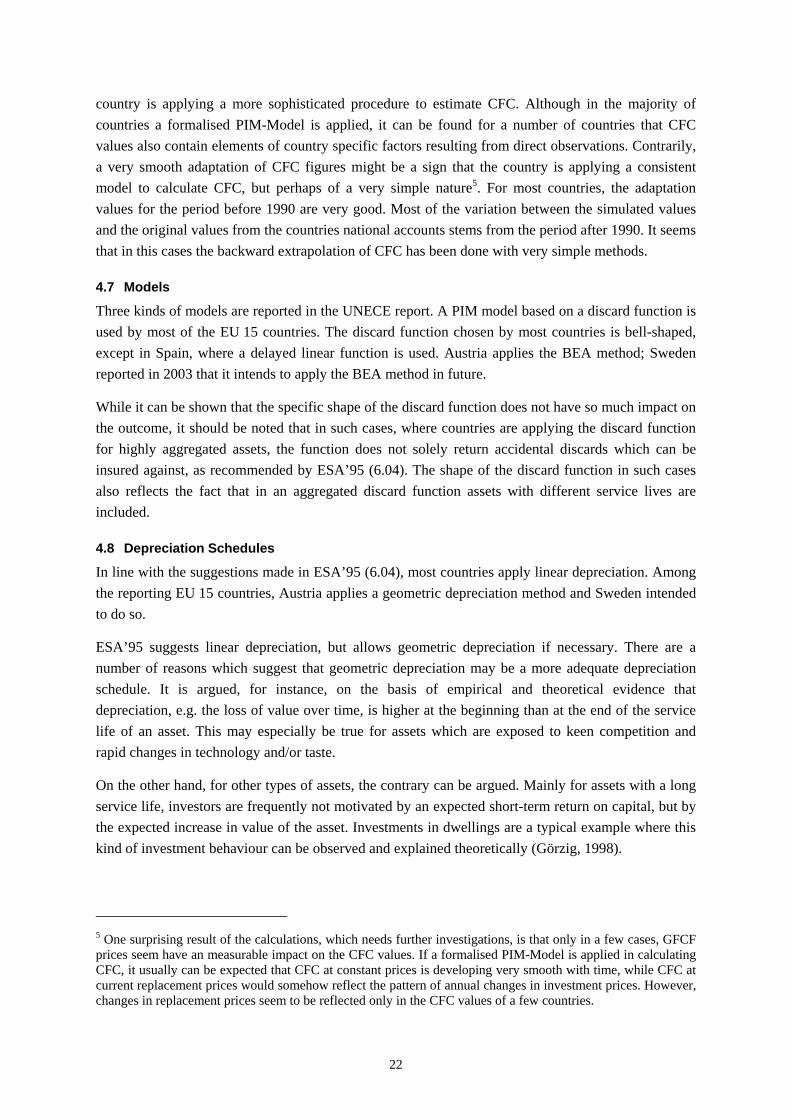
Table 9: Ranges of Implicit Service Life for Different Periods

Considering that the deviations of aggregate service lives are also influenced by compositional factors of GFCF, it can be concluded that, for most countries, service life estimates are fairly close together. However, even if the outlier Greece and the countries with extremely low service lives are ignored, the difference between a low service life of 25 years, e.g. for the Netherlands, and a high service life of 39 years, e.g. for Austria, is still quite high. The impact of this difference on capital stock estimates for these countries will be proportional to the relationship between service lives. This will exert a severe impact on productivity and profitability estimates.

The correlation between the CFC ratio and the estimated implicit service life assumptions is negative and considerably high (-0.53). However, this is mainly due to the extreme values for Greece4. The correlation without Greece is -0.17. Still, it seems that differences in the service life assumptions do contribute to the observed differences in CFC ratios between the countries.

While the model's primarily aim is to give some ideas on the implicit service live assumptions made in the countries, the comparison of CFC values as generated by the model with CFC values calculated in a country's national accounts may give some additional insight into the applied methods. In particular, the degree of adaptation does not necessarily qualify the simulation. A good adaptation of the trend of depreciation, accompanied by considerable annual variations, might be a sign that the

4 The high value for Greece is a result of a very low relation between CFC and GFCF in the national accounts for Greece, which can only be consistent with the observed growth rate of GFCF, if the service life is assumed to be very high. A reason for this might be the insufficient coverage of GFCF.

Country

Source: DIW Calculations. -

Average service lifeyears

Adaptation period for CFC

2004 1990 -

2004 1980 -

2004 1970 -

191818Luxembourg112020Denmark192020Portugal222424Belgium252729Netherlands282827UK282929Ireland303030Finland293235Germany313233France313333Spain303436Sweden363738Italy393838Austria555959Greece

22

country is applying a more sophisticated procedure to estimate CFC. Although in the majority of countries a formalised PIM-Model is applied, it can be found for a number of countries that CFC values also contain elements of country specific factors resulting from direct observations. Contrarily, a very smooth adaptation of CFC figures might be a sign that the country is applying a consistent model to calculate CFC, but perhaps of a very simple nature5. For most countries, the adaptation values for the period before 1990 are very good. Most of the variation between the simulated values and the original values from the countries national accounts stems from the period after 1990. It seems that in this cases the backward extrapolation of CFC has been done with very simple methods.

4.7 Models

Three kinds of models are reported in the UNECE report. A PIM model based on a discard function is used by most of the EU 15 countries. The discard function chosen by most countries is bell-shaped, except in Spain, where a delayed linear function is used. Austria applies the BEA method; Sweden reported in 2003 that it intends to apply the BEA method in future.

While it can be shown that the specific shape of the discard function does not have so much impact on the outcome, it should be noted that in such cases, where countries are applying the discard function for highly aggregated assets, the function does not solely return accidental discards which can be insured against, as recommended by ESA’95 (6.04). The shape of the discard function in such cases also reflects the fact that in an aggregated discard function assets with different service lives are included.

4.8 Depreciation Schedules

In line with the suggestions made in ESA’95 (6.04), most countries apply linear depreciation. Among the reporting EU 15 countries, Austria applies a geometric depreciation method and Sweden intended to do so.

ESA’95 suggests linear depreciation, but allows geometric depreciation if necessary. There are a number of reasons which suggest that geometric depreciation may be a more adequate depreciation schedule. It is argued, for instance, on the basis of empirical and theoretical evidence that depreciation, e.g. the loss of value over time, is higher at the beginning than at the end of the service life of an asset. This may especially be true for assets which are exposed to keen competition and rapid changes in technology and/or taste.

On the other hand, for other types of assets, the contrary can be argued. Mainly for assets with a long service life, investors are frequently not motivated by an expected short-term return on capital, but by the expected increase in value of the asset. Investments in dwellings are a typical example where this kind of investment behaviour can be observed and explained theoretically (Görzig, 1998).

5 One surprising result of the calculations, which needs further investigations, is that only in a few cases, GFCF prices seem have an measurable impact on the CFC values. If a formalised PIM-Model is applied in calculating CFC, it usually can be expected that CFC at constant prices is developing very smooth with time, while CFC at current replacement prices would somehow reflect the pattern of annual changes in investment prices. However, changes in replacement prices seem to be reflected only in the CFC values of a few countries.

23

5 Conclusions for the EU KLEMS Project Depreciation levels in the EU 15 countries vary considerably. However, there seems to be no unique economic factor to explain this. Economic explanations are not satisfactory. Methodological differences exist, but the causality is not clear-cut.

To improve the possibilities of explanation, it would be helpful to apply more standardised methods. The most important strategy for standardisation in the EU KLEMS project is the harmonisation of the asset and industry breakdown. A harmonised asset and industry breakdown will improve the possibilities to separate structural from methodological influences. However, additional questions arise:

Data It is important to make transparent, to what extent CFC is calculated in using series of

New investment, or

GFCF, which includes purchases and sales of used assets, or

Net additions to capital stock, which also includes changes in industry affiliation and premature scrapping.

Methodology Although it seems that there are a number of methodological differences between the countries' estimates of CFC, it is difficult to decide to what extent these differences do influence the estimated CFC values. Despite considerable methodological differences with respect to the discard function, the depreciation schedule, and the degree of disaggregation, for some of the countries, the resulting implicit service lives for total CFC for the countries seem to be surprisingly close together. The resulting values of total CFC seem to be comparatively robust against the wide range of different methodologies applied in the European countries. Before the background off the macro-economic policy aspects of the CFC calculations, this result can been helpful for an assessment of the reliability of total GDPs in the countries.

However, this result for overall CFC cannot exclude the possibility that there might be wide differences, if the comparison is made for individual industries. To improve the quality of productivity comparisons, researchers have suggested a standardisation of the methodologies applied. However, it has to be considered that any deviation from the methodology applied by a country might cause additional inconsistencies, especially if country specific information is left out. There certainly is no ideal solution to fulfil the demand for harmonisation in the EU KLEMS project on the one hand and to keep the country specific information on the other. A procedure, which circumvents some of these problems consists of two steps:

Instead of applying new investment in a PIM-Model, the country's present estimates of net additions to capital stock are treated like new investments.

A harmonised PIM-Model is applied for all countries, while leaving open the possibility for country specific service live assumptions.

24

References: BEA, 1999, Fixed Reproducible Tangible Wealth in the United States, 1925–94, U.S. Department of

Commerce, Bureau off Economic Analysis.

Bundesministerium der Finanzen, 2006, AfA-Tabelle für die allgemein verwendbaren Anlagegüter.

Cope, Jeff, 1998, Determining Asset Lives by Direct Survey, 2nd meeting of the Canberra Group on Capital Stock Estimates, Paris.

ESA 1995, European system of accounts,

EU KLEMS, 2005, Report on data availability, January 2005.

Görzig, Bernd, 1998, Determinanten von Abschreibungen, in: Kategorien der Volkswirtschaftlichen Gesamtrechnungen, Hrsg.: U.-P. Reich, C. Stahmer, K. Voy, Band 2, Zeit und Risiko.

Kirner, Wolfgang, 1968, Zeitreihen für das Anlagevermögen der Wirtschaftsbereiche in der Bundesrepublik Deutschland, DIW – Beiträge zur Strukturforschung, Heft 5, Berlin.

OECD, 1993, Methods Used by OECD Countries to Measure Stocks of Fixed Capital, National Accounts: Sources and Methods, No.2:

OECD, 2001, Measuring Capital, OECD Manual, Measurement of Capital Stocks, Consumption of Fixed Capital and Capital Services, OECD, 2001.

OECD, 2006, Source OCDE Annual National Accounts - volume I - Main aggregates Vol. 2005 release 02 -

Schmalwasser, Oda, 2001, Revision der Anlagevermögensrechnung 1991 bis 2001, in: Wirtschaft u. Statistik, 5, Wiesbaden

Statistics Netherlands, 2005, Dirk van den Bergen, Mark de Haan, Ron de Heij, Myriam Horsten, Measuring Capital in the Netherlands, OECD Working Party on National Accounts, Paris.

Statistisches Bundesamt, 2005, Statistical Yearbook for Foreign Countries, Wiesbaden.

UNECE, 2003, United nations economic commission for Europe, statistical division, conference of European statisticians, measurement of capital stock in transition economies, occasional paper 2003/1.

UNECE, 2004, UNECE/Eurostat/OECD meeting on national accounts, Survey of national practices in estimating service lives of capital assets.

West, Paul, 1998, The Direct Observation of Asset Lives, 2nd meeting of the Canberra Group on Capital Stock Estimates, Paris.

25

Annex 1: Data Used in Assessing Average Service Lives in the EU Countries

20042003200220012000199019801970CurrencyCountry

Gross fixed capital formation - current prices49,6848,5645,5447,6747,8830,7518,807,07mrd. euroAustria54,2651,6251,3952,8752,4536,5520,457,99mrd. euroBelgium

282,62270,70266,70264,03261,10163,9477,3030,90mrd. dkrDenmark28,2026,3226,5827,7325,7525,278,842,15mrd. euroFinland

315,96300,29290,55291,64280,67221,87101,4130,02mrd. euroFrance384,94384,38392,90422,88442,43322,99207,14107,02mrd. euroGermany42,4039,3033,7831,2928,729,041,740,26mrd. euroGreece36,2931,9629,0827,1125,376,793,550,49mrd. euroIreland

262,91249,59249,35240,56230,93146,3349,978,80mrd. euroItaly4,964,745,005,024,432,150,940,33mrd. euroLuxembourg

94,6490,7592,8694,6790,6855,7436,7416,37mrd. euroNetherlands30,5129,4932,1733,2632,4213,332,240,26mrd. euroPortugal

233,65211,33191,00176,51162,8180,7921,794,43mrd. euroSpain413,76392,84392,07395,62389,01328,87114,9642,05mrd. skrSweden190,06175,95172,56165,67161,81114,3043,2410,04mrd. ,UK

Gross fixed capital formation - constant chain linked prices (2000=100)

47,8247,5244,8047,1647,8836,6130,4220,80mrd. euroAustria53,1951,0351,3952,5852,4543,9435,1526,35mrd. euroBelgium



238,71233,90238,09235,24230,93198,65164,54137,98mrd. euroItaly4,684,524,824,884,432,621,791,39mrd. euroLuxembourg

86,1483,7086,7690,8990,6867,5954,5753,07mrd. euroNetherlands28,2827,9331,0032,6732,4219,6014,6510,12mrd. euroPortugal


Consumption of fixed capital - current replacement prices33,7332,4631,6230,6729,2018,9810,393,97mrd. euroAustria44,9843,0041,2639,9737,6221,9512,684,23mrd. euroBelgium



186,15176,08168,93160,50152,3686,8925,554,01mrd. euroItaly0,003,063,062,882,621,480,680,33mrd. euroLuxembourg73,2271,3369,4365,8761,5937,6421,156,63mrd. euroNetherlands24,1023,2922,5321,4920,097,971,220,20mrd. euroPortugal


Source: OECD National Accounts. - DIW Calculations. -

26

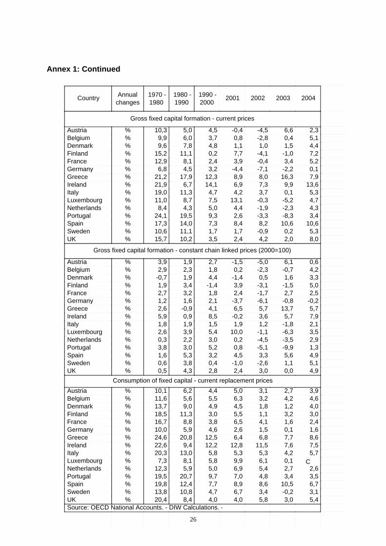
Annex 1: Continued

20042003200220012000

1990 -1990

1980 -1980

1970 -changesAnnualCountry

Gross fixed capital formation - current prices

2,36,6-4,5-0,44,55,010,3%Austria5,10,4-2,80,83,76,09,9%Belgium4,41,51,01,14,87,89,6%Denmark7,2-1,0-4,17,70,211,115,2%Finland5,23,4-0,43,92,48,112,9%France0,1-2,2-7,1-4,43,24,56,8%Germany7,916,38,08,912,317,921,2%Greece

13,69,97,36,914,16,721,9%Ireland5,30,13,74,24,711,319,0%Italy4,7-5,2-0,313,17,58,711,0%Luxembourg4,3-2,3-1,94,45,04,38,4%Netherlands3,4-8,3-3,32,69,319,524,1%Portugal

10,610,68,28,47,314,017,3%Spain5,30,2-0,91,71,711,110,6%Sweden8,02,04,22,43,510,215,7%UK

Gross fixed capital formation - constant chain linked prices (2000=100)

0,66,1-5,0-1,52,71,93,9%Austria4,2-0,7-2,30,21,82,32,9%Belgium3,31,60,5-1,44,41,9-0,7%Denmark5,0-1,5-3,13,9-1,43,41,9%Finland2,52,7-1,72,41,83,22,7%France

-0,2-0,8-6,1-3,72,11,61,2%Germany5,713,75,76,54,1-0,92,6%Greece7,95,73,6-0,28,50,95,9%Ireland2,1-1,81,21,91,51,91,8%Italy3,5-6,3-1,110,05,43,92,6%Luxembourg2,9-3,5-4,50,23,02,20,3%Netherlands1,3-9,9-5,10,85,23,03,8%Portugal4,95,63,34,53,25,31,6%Spain5,11,1-2,6-1,00,43,80,6%Sweden4,90,03,02,42,84,30,5%UK

Consumption of fixed capital - current replacement prices3,92,73,15,04,46,210,1%Austria4,64,23,26,35,55,611,6%Belgium4,01,21,84,54,99,013,7%Denmark3,03,21,15,53,011,318,5%Finland2,41,64,16,53,88,816,7%France1,60,11,52,64,65,910,0%Germany8,67,76,86,412,520,824,6%Greece7,57,611,512,812,29,422,6%Ireland5,74,25,35,35,813,020,3%Italy

C0,16,19,95,88,17,3%Luxembourg2,62,75,46,95,05,912,3%Netherlands3,53,44,87,09,720,719,5%Portugal6,710,58,68,97,712,419,8%Spain3,1-0,23,46,74,710,813,8%Sweden5,43,05,84,04,08,420,4%UK

Source: OECD National Accounts. - DIW Calculations. -

27

Annex 2: Elements of the DIW Capital Stock Model

1

( )M

net nett t i

i

K I g i−=

= ∗∑ Net stock at the beginning of the year

1( )

M

t t ii

K I g i−=

= ∗∑ Gross stock at the beginning of the year

1con net nett t t tD K K I+= − + CFC at constant prices

/con cont t t tD CFC I I= ∗ CFC at current (replacement) prices

11 11 1

( ) / exp( p pg i c MM i i

⎡ − ⎤⎛ ⎞= + ∗ ∗ +⎜ ⎟⎢ ⎥+ − −⎝ ⎠⎣ ⎦ Survival function

1( ) ( ) ( )h i g i g i= − − Mortality function

1( ) ( )

Mnet net

ig i h i

=

= ∑ Net value function

( )( )M

net

k i

h kh ik=

= ∑ Depreciation function

Icon = Vintage of GFCF at constant prices I = Vintage of GFCF at current prices Dcon = CFC at constant prices D = CFC at replacement prices M = Maximum service life of a vintage of an asset. Used in the

survival function. c = Steepness of the mortality function. Used in the survival

function. Is assumed to have the value of 3. p = Skewness of the mortality function. Used in the survival function.

Is assumed to have the value of 0.6. i = Actual service life of a piece of a vintage of GFCF. t = Year.

28

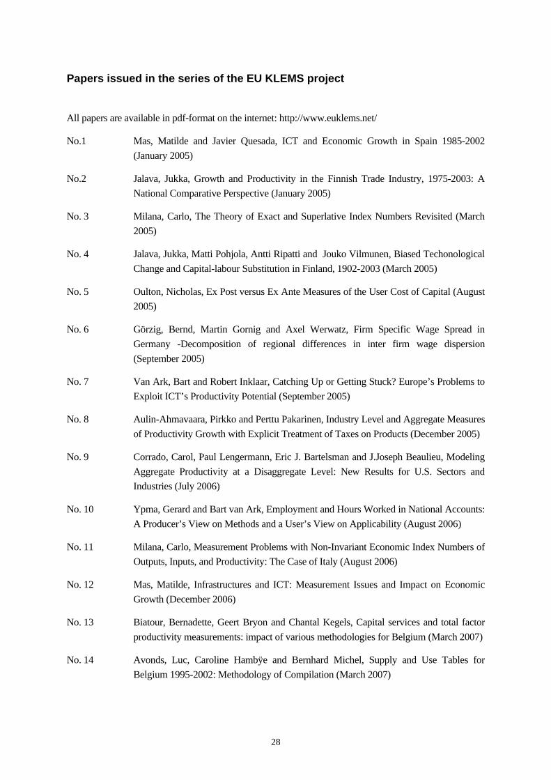
Papers issued in the series of the EU KLEMS project

All papers are available in pdf-format on the internet: http://www.euklems.net/

No.1 Mas, Matilde and Javier Quesada, ICT and Economic Growth in Spain 1985-2002 (January 2005)

No.2 Jalava, Jukka, Growth and Productivity in the Finnish Trade Industry, 1975-2003: A National Comparative Perspective (January 2005)

No. 3 Milana, Carlo, The Theory of Exact and Superlative Index Numbers Revisited (March 2005)

No. 4 Jalava, Jukka, Matti Pohjola, Antti Ripatti and Jouko Vilmunen, Biased Techonological Change and Capital-labour Substitution in Finland, 1902-2003 (March 2005)

No. 5 Oulton, Nicholas, Ex Post versus Ex Ante Measures of the User Cost of Capital (August 2005)

No. 6 Görzig, Bernd, Martin Gornig and Axel Werwatz, Firm Specific Wage Spread in Germany -Decomposition of regional differences in inter firm wage dispersion (September 2005)

No. 7 Van Ark, Bart and Robert Inklaar, Catching Up or Getting Stuck? Europe’s Problems to Exploit ICT’s Productivity Potential (September 2005)

No. 8 Aulin-Ahmavaara, Pirkko and Perttu Pakarinen, Industry Level and Aggregate Measures of Productivity Growth with Explicit Treatment of Taxes on Products (December 2005)

No. 9 Corrado, Carol, Paul Lengermann, Eric J. Bartelsman and J.Joseph Beaulieu, Modeling Aggregate Productivity at a Disaggregate Level: New Results for U.S. Sectors and Industries (July 2006)

No. 10 Ypma, Gerard and Bart van Ark, Employment and Hours Worked in National Accounts: A Producer’s View on Methods and a User’s View on Applicability (August 2006)

No. 11 Milana, Carlo, Measurement Problems with Non-Invariant Economic Index Numbers of Outputs, Inputs, and Productivity: The Case of Italy (August 2006)

No. 12 Mas, Matilde, Infrastructures and ICT: Measurement Issues and Impact on Economic Growth (December 2006)

No. 13 Biatour, Bernadette, Geert Bryon and Chantal Kegels, Capital services and total factor productivity measurements: impact of various methodologies for Belgium (March 2007)

No. 14 Avonds, Luc, Caroline Hambÿe and Bernhard Michel, Supply and Use Tables for Belgium 1995-2002: Methodology of Compilation (March 2007)

29

No. 15 Biatour, Bernadette, Jeroen Fiers, Chantal Kegels and Bernhard Michel, Growth and Productivity in Belgium (March 2007)

No. 16 Timmer, Marcel, Gerard Ypma and Bart van Ark, PPPs for Industry Output: A New Dataset for International Comparisons (March 2007)

No. 17 Görzig, Bernd, Depreciation in EU Member States: Empirical and Methodological Differences (April 2007)

depreciation in eu member states: empirical and ... · 1 depreciation in eu member states:...

Documents