dependable computing on inexact …cccp.eecs.umich.edu/theses/dskhudia-thesis.pdfdependable...
TRANSCRIPT

DEPENDABLE COMPUTING ON INEXACTHARDWARE THROUGH ANOMALY DETECTION
by
Daya Shanker Khudia
A dissertation submitted in partial fulfillmentof the requirements for the degree of
Doctor of Philosophy(Computer Science and Engineering)
in The University of Michigan2015
Doctoral Committee:
Professor Scott Mahlke, ChairAssistant Professor Jason MarsAssociate Professor Thomas WenischAssociate Professor Zhengya Zhang

c© Daya Shanker Khudia 2015
All Rights Reserved

To my family
ii

ACKNOWLEDGEMENTS
Thank you most of all to my adviser, Prof. Scott Mahlke. He has been very patient and
encouraging through the thick and thin of PhD life. This dissertation would not be possible
without his guidance and support. During the course of this dissertation, he always came up
with brilliant suggestions on what to try next whenever I was stuck on technical problems.
A huge thank you to the rest of my dissertation committee Prof. Jason Mars, Prof.
Thomas Wenisch and Prof. Zhengya Zhang for taking their valuable time in evaluating this
dissertation. Their critical comments and suggestion really helped me in improving my
work for ISCA15 conference and for the final chapter.
Many thanks to Prof. Valeria Bertacco for all the help in the first year of my graduate
studies. My sincere thanks goes to Dr. Andrew DeOrio, Dr. Debapriya Chaterjee and
Dr. Andrea Pellegrini for getting me started with the research process. I thank them for
teaching me the tricks and trades of the research process from a student’s point of view.
A profound thanks to fellow CCCP members Yongjun Park, Hyoun Kyu Cho, Ankit
Sethia, Gaurav Chadha, Anoushe Jamshidi, Mehrzad Samadi, Andrew Lukefahr, Shruti
Padmanabha, Janghaeng Lee, Jason Park, John Kloosterman, Babak Zamirai and Jiecao
Yu for all their help and keeping things interesting in the office. A special thank you to
Mehrzad–the funniest guy in the office–for help with the final project and to Andrew for
iii

keeping all the servers running so that I could run my simulations.
I have had the luck of having amazing friends in Ann Arbor. I share wonderful mem-
ories with them over evening tea, card games and road trips that I will cherish throughout
my life. I would like to thank Abhayendra Singh for always having and sharing informa-
tion on a broad range of topics, Gaurav Pandey for imparting wisdom in various situations,
Gaurav Chadha for taking all the jokes in the right spirit, Ritesh Parikh for filling in the
silences by being the chatter box, Shweta Srivastva for being the first one to get my jokes,
Ankit Sethia for all the help from the very beginning of graduate studies, Divya Golchha
for going to Bollywood movies with me when everyone else doubted my movie choice,
Mukesh Bachhav for making me laugh by trying to be funny and failing, Megha Dubey
for all the interesting discussions over afternoon coffee and good food at numerous occa-
sions. I would also like to thank my roommate Ashutosh Parkhi for all the technical and
non-technical discussions and Anand Geteey for being so easy to share a house with. Many
thanks to Animesh Banerjee, Anchal Agarwal, Ayan Das and Vivek Joshi for being always
ready for parties. I thank Ujjwal Jain and Biruk Mammo for all the fun activities. A lot of
the memories made in Ann Arbor will linger on for a long a time.
I thank Aasheesh Kolli for listening to my random stories and for introducing me to
Ultimate Frisbee, Shruti Padmanabha for being such a good sport with everything, Silky
Arora and Mohit Nahata for making my stupid jokes seem much funnier than they really
were, Neha Agarwal for showing sincere interest in discussing problems and Shaizeen Aga
for inspiring by being hard working and meticulous.
And last but not the least, my heartfelt thank you to my parents and my siblings for
always being there. Their unconditional love and support is beyond words.
iv
TABLE OF CONTENTS
DEDICATION . . . . . . . . . . . . . . . . . . . . . . . . . . . . . . . . . . . ii
ACKNOWLEDGEMENTS . . . . . . . . . . . . . . . . . . . . . . . . . . . . iii
LIST OF FIGURES . . . . . . . . . . . . . . . . . . . . . . . . . . . . . . . . viii
LIST OF TABLES . . . . . . . . . . . . . . . . . . . . . . . . . . . . . . . . . xiv
ABSTRACT . . . . . . . . . . . . . . . . . . . . . . . . . . . . . . . . . . . . . . xv
CHAPTER
I. Introduction . . . . . . . . . . . . . . . . . . . . . . . . . . . . . . . . . 1
1.1 Low-cost Reliability . . . . . . . . . . . . . . . . . . . . . . . . . 31.2 Quality Controlled Results . . . . . . . . . . . . . . . . . . . . . 61.3 Contributions . . . . . . . . . . . . . . . . . . . . . . . . . . . . 9
II. Efficient Soft Error Protection using Profile Information . . . . . . . . 11
2.1 Introduction . . . . . . . . . . . . . . . . . . . . . . . . . . . . . 122.2 Background and Motivation . . . . . . . . . . . . . . . . . . . . . 16
2.2.1 Soft Error Rate (SER) . . . . . . . . . . . . . . . . . . 162.2.2 Instruction Duplication . . . . . . . . . . . . . . . . . . 172.2.3 Proposed Solution Landscape . . . . . . . . . . . . . . 192.2.4 Opportunities for Profile Based Duplication . . . . . . . 21
2.3 Proposed Solution . . . . . . . . . . . . . . . . . . . . . . . . . . 222.3.1 Overview of proposed solution . . . . . . . . . . . . . . 232.3.2 Overhead Reduction Without Losing Coverage . . . . . 252.3.3 Software Symptom Generation using Value Profiling . . 29
2.4 Experimental Setup . . . . . . . . . . . . . . . . . . . . . . . . . 312.4.1 Compiler Passes . . . . . . . . . . . . . . . . . . . . . 312.4.2 Fault Injection Framework . . . . . . . . . . . . . . . . 322.4.3 Recovery Support . . . . . . . . . . . . . . . . . . . . . 35
v

2.4.4 Benchmarks . . . . . . . . . . . . . . . . . . . . . . . . 362.5 Experimental Results . . . . . . . . . . . . . . . . . . . . . . . . 36
2.5.1 Silent Stores . . . . . . . . . . . . . . . . . . . . . . . 362.5.2 Performance Overheads and Fault Coverage . . . . . . . 382.5.3 Contributions of Each Technique . . . . . . . . . . . . . 41
2.6 Related Work . . . . . . . . . . . . . . . . . . . . . . . . . . . . 422.7 Conclusions . . . . . . . . . . . . . . . . . . . . . . . . . . . . . 46
III. Low Cost Control Flow Protection Using Abstract Control Signatures . 47
3.1 Introduction . . . . . . . . . . . . . . . . . . . . . . . . . . . . . 483.2 Background and Motivation . . . . . . . . . . . . . . . . . . . . . 51
3.2.1 Fault Detection . . . . . . . . . . . . . . . . . . . . . . 513.2.2 Control Flow Errors . . . . . . . . . . . . . . . . . . . 533.2.3 Signature Based Techniques and Associated Overheads . 54
3.3 Abstract Control Signatures . . . . . . . . . . . . . . . . . . . . . 563.3.1 Design of ACS . . . . . . . . . . . . . . . . . . . . . . 583.3.2 Calculating Balancing Increments . . . . . . . . . . . . 623.3.3 Error Detection Analysis . . . . . . . . . . . . . . . . . 643.3.4 Insertion of Checking Instructions . . . . . . . . . . . . 663.3.5 Optimization for Loops . . . . . . . . . . . . . . . . . . 663.3.6 Call and Return Instructions . . . . . . . . . . . . . . . 67
3.4 Experimental Setup . . . . . . . . . . . . . . . . . . . . . . . . . 693.4.1 Compiler Transformations . . . . . . . . . . . . . . . . 693.4.2 Benchmarks . . . . . . . . . . . . . . . . . . . . . . . . 703.4.3 Fault Injection Campaign . . . . . . . . . . . . . . . . . 703.4.4 Recovery Support . . . . . . . . . . . . . . . . . . . . . 74
3.5 Experimental Evaluation and Analysis . . . . . . . . . . . . . . . 753.5.1 Fault Detection Latency . . . . . . . . . . . . . . . . . 773.5.2 Analysis of SDCs . . . . . . . . . . . . . . . . . . . . . 783.5.3 Data and Control Flow Protection . . . . . . . . . . . . 793.5.4 Discussion and Limitations . . . . . . . . . . . . . . . . 80
3.6 Related Work . . . . . . . . . . . . . . . . . . . . . . . . . . . . 813.7 Conclusions . . . . . . . . . . . . . . . . . . . . . . . . . . . . . 85
IV. Harnessing Soft Computations for Low-budget Fault Tolerance . . . . 86
4.1 Introduction . . . . . . . . . . . . . . . . . . . . . . . . . . . . . 874.2 Motivation . . . . . . . . . . . . . . . . . . . . . . . . . . . . . . 90
4.2.1 Soft Computations . . . . . . . . . . . . . . . . . . . . 904.2.2 Silent Data Corruptions . . . . . . . . . . . . . . . . . 92
4.3 Solution: Analysis and Design . . . . . . . . . . . . . . . . . . . 944.3.1 Overview . . . . . . . . . . . . . . . . . . . . . . . . . 944.3.2 Recomputing State Variables . . . . . . . . . . . . . . . 994.3.3 Expected Value Checks . . . . . . . . . . . . . . . . . . 100
vi

4.4 Experimental Setup . . . . . . . . . . . . . . . . . . . . . . . . . 1044.4.1 Source Code Transformations . . . . . . . . . . . . . . 1044.4.2 Benchmarks and Fidelity Measures . . . . . . . . . . . 1064.4.3 Fault Model and Injection Experiments . . . . . . . . . 1074.4.4 Recovery Support . . . . . . . . . . . . . . . . . . . . . 110
4.5 Experimental Evaluation and Analysis . . . . . . . . . . . . . . . 1114.6 Related Work . . . . . . . . . . . . . . . . . . . . . . . . . . . . 1164.7 Conclusions . . . . . . . . . . . . . . . . . . . . . . . . . . . . . 119
V. Rumba: An Online Quality Management System for ApproximateComputing . . . . . . . . . . . . . . . . . . . . . . . . . . . . . . . . . . 121
5.1 Introduction . . . . . . . . . . . . . . . . . . . . . . . . . . . . . 1225.2 Challenges and Opportunities . . . . . . . . . . . . . . . . . . . . 126
5.2.1 Challenges of Managing Output Quality . . . . . . . . . 1265.2.2 Rumba’s Design Principles . . . . . . . . . . . . . . . . 130
5.3 Design of Rumba . . . . . . . . . . . . . . . . . . . . . . . . . . 1325.3.1 Overview . . . . . . . . . . . . . . . . . . . . . . . . . 1325.3.2 Light-weight Error Prediction . . . . . . . . . . . . . . 1345.3.3 Low-overhead Recovery . . . . . . . . . . . . . . . . . 1395.3.4 Online Tuning . . . . . . . . . . . . . . . . . . . . . . 1395.3.5 Error Detector Placement . . . . . . . . . . . . . . . . . 141
5.4 Experimental Setup . . . . . . . . . . . . . . . . . . . . . . . . . 1425.5 Evaluation . . . . . . . . . . . . . . . . . . . . . . . . . . . . . . 144
5.5.1 Output Quality . . . . . . . . . . . . . . . . . . . . . . 1445.5.2 Energy Consumption and Speedup . . . . . . . . . . . . 1485.5.3 Case Studies . . . . . . . . . . . . . . . . . . . . . . . 151
5.6 Related Work . . . . . . . . . . . . . . . . . . . . . . . . . . . . 1535.7 Conclusions . . . . . . . . . . . . . . . . . . . . . . . . . . . . . 157
VI. Neural Accelerator and Checker Design Space Exploration . . . . . . . 158
6.1 Introduction . . . . . . . . . . . . . . . . . . . . . . . . . . . . . 1596.2 Exploration Setup . . . . . . . . . . . . . . . . . . . . . . . . . . 1606.3 Experimental Results . . . . . . . . . . . . . . . . . . . . . . . . 1616.4 Conclusions . . . . . . . . . . . . . . . . . . . . . . . . . . . . . 165
VII. Conclusions and Future Directions . . . . . . . . . . . . . . . . . . . . 166
BIBLIOGRAPHY . . . . . . . . . . . . . . . . . . . . . . . . . . . . . . . . . 170
vii

LIST OF FIGURES
Figure
1.1 A high-level flow diagram of the overall process. Compilation phase per-forms profiling and an analysis of vulnerable parts of an application. Italso analyzes an application, with the help of developer provided anno-tations, for approximate parts. The checkers are inserted as a part of thecompilation process. Recovery for transient errors or to get better qualityresults is initiated at runtime. . . . . . . . . . . . . . . . . . . . . . . . . 8
2.1 Duplicating instructions in a single thread of execution: Part (a) showsthe original code and Part (b) shows the code after the duplicated instruc-tions are inserted. Solid edges represent the data flow edges and dashededges represent control flow edges. In (b), underlined nodes are dupli-cated nodes, and C and B nodes represent compare and branch instruc-tions to compare the results from duplicated and original dataflow chains.The node with dashed outline is a symptom generating instruction. . . . . 18
2.2 The trade-off between overhead and fault coverage from two existingfault detection schemes: symptom-based detection and instruction duplication-based detection. Also indicated is the region of the solution space targetedby our proposed technique. Our solution is aiming to provide between90% and 99% coverage with little overhead. The dashed horizontal linesshow user-visible failure rate for a single chip in a 16nm technologynode with aggressive voltage scaling. This is a conceptual plot and is notto scale. . . . . . . . . . . . . . . . . . . . . . . . . . . . . . . . . . . . 20
2.3 This Figure shows the flow of application compilation. LLVM bit-codeis the internal representation of the LLVM compiler infrastructure. Ourproposed solution operates at the LLVM bit-code level. Classification andanalysis phases identify vulnerable parts of an application, and then theduplication phase protects the most vulnerable instructions by duplicatingcode. . . . . . . . . . . . . . . . . . . . . . . . . . . . . . . . . . . . . 23
viii
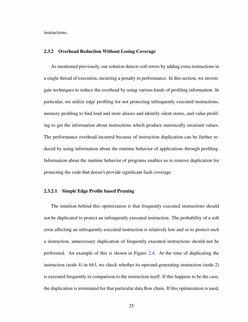
2.4 This Figure shows an example where execution frequency-based opti-mization is effective. The solid edges represent data flow edges anddashed edges represent control flow edges. Control flow edges are an-notated with the execution frequency of the edge obtained using a profilerun. Underlined numbers represent duplicated instructions. While du-plicating an instruction in basic block bb3, if its operands’ parent basicblock is executed 100 times more frequently, then we don’t duplicate itsoperand. . . . . . . . . . . . . . . . . . . . . . . . . . . . . . . . . . . 26
2.5 This Figure represents the control and data flow graphs for an examplecode. Solid arrows represent data flow edges and dashed edges representcontrol flow edges. In part (a), instructions 1 and 2 are both duplicated(seen underlined), with comparisons (C) and branches (B) to recoverycode if a comparison fails. L represents a load instruction. If a silentstore is on the path of the recursive producer chain, then the duplicationprocess is terminated at that store and no source operands of the store areduplicated, as seen in part (b). The store instruction ’S’ is assumed to bea silent store for this example. . . . . . . . . . . . . . . . . . . . . . . . 28
2.6 The effect of the value profiling on the instruction duplication process.Part (a) shows duplication without considering value profiling while part(b) shows duplication if value profiling is taken into account. Instruction3 is assumed to generate the value ’0’ more than 99% of the time, andan extra comparison(C3,0) is added accordingly, jumping to additionalrecovery code if this comparison fails. Underlined instructions are dupli-cates, branches are indicated with ’B’, and comparisons with ’C’. . . . . . 29
2.7 The % Dynamic silent stores bar shows dynamic silent stores as a per-centage of total dynamic stores in a benchmark. The high percentage ofsilent stores in some benchmarks suggest that their presence can be ex-ploited for intelligent code duplication. The % Overhead reduction barshows the reduction in performance overhead if silent store optimizationis used while duplicating instructions. Notice that the benchmarks show-ing a large percentage of silent stores also show a significant reduction inoverhead. . . . . . . . . . . . . . . . . . . . . . . . . . . . . . . . . . . 37
2.8 Overhead comparison among full duplication, profile oblivious duplica-tion, and profile aware duplication. In full duplication, duplication is notterminated at safe instructions and all branches are also protected. Al-though profile oblivious duplication uses safe instructions, profiling infor-mation is not utilized. This represents a system equivalent to Shoestring.Profile-aware duplication uses safe instructions as well as profiling infor-mation. . . . . . . . . . . . . . . . . . . . . . . . . . . . . . . . . . . . 38
2.9 Coverage breakdown for full duplication (full-dup), profile oblivious du-plication (pro-oblivi) and profile aware duplication (pro-aware). . . . . . 39
ix

2.10 The profile-oblivious column is the baseline overhead. The reductionin overhead if we use the silent store optimization and edge profilinginformation is shown in the ‘Sl-st and edge profile aware’ column. Thevalue profile aware column shows the reduction in overhead if we usevalue profile in comparison to our baseline. . . . . . . . . . . . . . . . . 42
2.11 The pro-oblivi column shows the coverage breakdown for our baseline. The coverage breakdown if we use silent store optimization and edgeprofile information is shown in the sl-edge-aware column. The val-awarecolumn shows the coverage breakdown for value profile aware code du-plication. . . . . . . . . . . . . . . . . . . . . . . . . . . . . . . . . . . 43
3.1 Control flow target errors are ∼2.5x as likely to cause incorrect executions. 523.2 Control Flow Target Errors: Corruption of branch target can result in
nearby (Type A) or far away (Type B) displacement of control flow. . . . 533.3 Basic signature scheme: If the correct control flow transfer takes place,
G at dest_BB would be equal to s2 otherwise not. . . . . . . . . . . . . . 543.4 Abstract signatures: The whole program is divided into regions at a higher
abstraction level. Such regions are enclosed by dashed light blue (grey)lines in this Figure. Every region is assigned a signature. Every abstractregion updates its signature based on the control transfers among the BBsinside it. These signatures are only checked in other abstract regions. . . . 56
3.5 Intervals in the Figure are shown by enclosed dashed light blue (gray)lines. This Figure shows two intervals for a control flow graph that has anested loop. . . . . . . . . . . . . . . . . . . . . . . . . . . . . . . . . . 60
3.6 Every interval is associated with a signature. In our scheme, signatureare simple counters. The signature is initialized in the header and incre-mented by 1 in other blocks. The signature checks are made in the BBsthat are destination BBs of exits out of an interval. . . . . . . . . . . . . 61
3.7 The extra increments required to be inserted along control flow edges isshown. This balances out signature values at the exits out of an interval. . 62
3.8 Optimizing signature checking for loops: The checks on signatures aremoved out of loops to exit blocks so that they are not executed in eachiteration. . . . . . . . . . . . . . . . . . . . . . . . . . . . . . . . . . . 66
3.9 Handling call and return instructions. Instructions in bold represent theinserted instructions. . . . . . . . . . . . . . . . . . . . . . . . . . . . . 68
3.10 The incorrect executions as a percentage of unmasked faults caused bydisturbance in control flow targets. Faults are injected in register file aswell as branch targets. . . . . . . . . . . . . . . . . . . . . . . . . . . . 71
3.11 The performance (Runtime on simulated core) overhead for all techniques.. . . . . . . . . . . . . . . . . . . . . . . . . . . . . . . . . . . . . . . 75
3.12 CFCSS bar shows the fault coverage for CFCSS and CFCSS_ivl showsthe fault coverage with checking inserted using interval information. ACS_-w/o_calls_rets shows the fault coverage without protection for calls/re-turns and ACS_w/o_calls_rets shows the fault coverage if calls/returnsare also protected. . . . . . . . . . . . . . . . . . . . . . . . . . . . . . 76
x
3.13 Comparison of fault detection latency with CFCSS. The fault detectionlatency is not adversely affected. . . . . . . . . . . . . . . . . . . . . . . 77
3.14 Performance overhead and fault coverage for complete data and controlflow protection. . . . . . . . . . . . . . . . . . . . . . . . . . . . . . . . 80
4.2 SDCs are divided into acceptable SDCs and unacceptable SDCs. Unac-ceptable SDCs are further divided into the ones due to large and smallinstruction output value changes. Soft checks using expected values candetect unacceptable SDCs (up to 14% of total SDCs) due to large instruc-tion output value change. . . . . . . . . . . . . . . . . . . . . . . . . . . 93
4.3 The code snippet from mp3dec (mad) [50] benchmark. The variables thatare dependent on their own values in the previous iterations are under-lined. A corruption in such variables is more likely to result in unaccept-able outputs. . . . . . . . . . . . . . . . . . . . . . . . . . . . . . . . . . 95
4.4 The code snippet from Figure 4.3 with crc variable duplicated. For thesake of brevity, the duplication of other state variables (those shown inFigure 4.3) is not shown in this figure. Variables postfixed with D areduplicated variables. . . . . . . . . . . . . . . . . . . . . . . . . . . . . 96
4.5 The code snippet from Figure 4.3 with expected value check inserted onvariable tableVal. Assume that the value generated lie within the range[V1, V2] (Obtained by profiling). This is a simple example of insertingvalue checks and more detailed examples are shown later in Section 4.3.3. 97
4.6 Instruction duplication in a single thread of execution. Instructions markedwith double circle are duplicated instructions. The instruction markedwith ld is a load instruction. We do not duplicate loads to save on mem-ory traffic. . . . . . . . . . . . . . . . . . . . . . . . . . . . . . . . . . . 98
4.7 Depending on the generated values, one of the three different types ofvalue checks can be inserted. Part (a) shows a single value check insertedif a single value is frequently generated by an instruction. If two valuesare most frequently generated, the check in part (b) is inserted. However,if the values generated lie in a range, a range check as shown in part (c)is inserted. . . . . . . . . . . . . . . . . . . . . . . . . . . . . . . . . . 99
4.8 Optimization 1 for long producer chains: this figure shows an exampleof a case where multiple instructions in the producer chain of an instruc-tion are amenable for value checks. In order to minimize on number ofchecks, value check should only be inserted for an instruction lower inthe producer chain. . . . . . . . . . . . . . . . . . . . . . . . . . . . . . 101
4.9 Optimization 2 for long producer chains: if an instruction amenable tovalue check is encountered in producer chain, the duplication of producerchain of critical variables is terminated at that point and a value check(vChk) is inserted as shown. . . . . . . . . . . . . . . . . . . . . . . . . . 101
4.10 shows the total number of state variables, duplicated instructions and in-serted value checks as a fraction of the total static IR instructions. Thestatic code duplication and expected value checks are not more than 12%of the total static IR instructions. . . . . . . . . . . . . . . . . . . . . . . 107
xi

4.11 The fault outcome distribution among different categories is shown. Col-umn original shows the distribution for original unmodified code. Thefault distribution with code duplication and code duplication along withvalue checks is shown in Dup only and Dup + val chks, respectively. . . . 110
4.12 Performance overhead of checking by 1) duplicating the producer chainof state variables. 2) duplicating the producer chain as well as insertingvalue checks wherever necessary. . . . . . . . . . . . . . . . . . . . . . . 111
4.13 Each column represents the silent data corruptions as a percentage of totalfaults. The stacks in each column further divide the silent corruptionsbetween acceptable program outputs and unacceptable data corruptions. . 112
5.1 Typical cumulative distribution function of errors generated by approxi-mation techniques. A large number of output elements have small errorswhile a few output elements have large errors. . . . . . . . . . . . . . . . 126
5.2 An example of variation in image quality with the changing distributionof errors. Subfigure (a) is the original image without any errors. Tenpercent of the pixels in (b) have 100% error while the rest of the pixels areintact. All pixels in (c) have 10% error. Although these two images havethe same average quantitative output quality (90%), errors in Subfigure(b) are more noticeable. . . . . . . . . . . . . . . . . . . . . . . . . . . . 127
5.3 Mosaic application’s output error for 800 different images of flowers.This data shows that the output quality is highly input-dependent. . . . . . 129
5.4 Exact output, approximate output and relative errors in the approximateoutput. The relative errors in the approximate output are higher for someinputs than the others and are more easily predictable than the output itself.130
5.5 A high-level block diagram of the Rumba system. The offline compo-nents determine the suitability of an application for the Rumba accelera-tion environment. The online components include detection and recoverymodules. The approximation accelerator communicates a recovery bitcorresponding to the ID of the elements to recompute with the CPU via arecovery queue. . . . . . . . . . . . . . . . . . . . . . . . . . . . . . . . 132
5.6 A decision tree with a depth of 3 in decision nodes. For this example,it predicts errors based on two inputs. The leaf nodes (gray) give theapproximation errors. The coefficients (cis and vis) are determined byoffline training. . . . . . . . . . . . . . . . . . . . . . . . . . . . . . . . 136
5.7 Hardware for the approximation error predictors. . . . . . . . . . . . . . 1385.8 An example of overlapping the re-computation of elements by the CPU
with the approximation accelerator. For example, a large error is detectedin iteration 0 by the accelerator and the CPU recomputes this iterationwhile accelerator is working on the execution of iteration 1 and 2. . . . . 138
5.9 Shows the design choices for the relative placement of input-based detec-tors with respect to the accelerator. Configuration in part (a) adds delay,thus impacting overall performance, in the path to invoking accelerator.Configuration in part (b) wastes energy on invocations of the acceleratorthat have large error. . . . . . . . . . . . . . . . . . . . . . . . . . . . . . 141
5.10 Output error with respect to the number of output elements fixed. . . . . . 145
xii

5.11 False positives at 90% target output quality. Ideal have zero false pos-itives. A low number of false positives for linearErrors and treeErrorsindicate their effectiveness in detecting large approximation errors. . . . . 146
5.12 The number of elements that are required to be re-executed for a 90%target output quality. . . . . . . . . . . . . . . . . . . . . . . . . . . . . 148
5.13 Relative coverage of large errors at 90% target output quality. Ideal has100% coverage. . . . . . . . . . . . . . . . . . . . . . . . . . . . . . . . 149
5.14 Energy consumption of Rumba, including the cost of re-computation andthe energy used for the prediction of large approximation errors. treeEr-rors saves 2.2x energy while the unchecked NPU saves 3.2x energy. . . . 150
5.15 Speedup of each technique with respect to the CPU baseline. Rumba(linearErrors or treeErrors) maintains the same speedup (2.2x) as the NPU.151
5.16 Time used by error prediction models in comparison to the NPU. Thisis normalized with respect to the NPU. Error prediction model are fasterin all the cases, hence, the accelerator never needs to wait for the errorprediction model to finish execution. . . . . . . . . . . . . . . . . . . . . 152
5.17 Energy consumption vs target error rate for fft. . . . . . . . . . . . . . . . 1535.18 The approximation accelerator and the CPU work in tandem. The CPU
works on re-computing detected large error iterations while the accelera-tor continues with the execution. In this case, 0.33 is the tuning thresholdused to achieve 10% target error rate. . . . . . . . . . . . . . . . . . . . . 154
6.1 Shows the steps to train an error predictor. . . . . . . . . . . . . . . . . . 1606.2 Error versus cost design points by pairing of different NPU configura-
tions with different configurations of the NN checker and decision treechecker of different depths. This data is for Blackscholes benchmark andonly some selective configurations are labeled and shown. All pairing ofconfigurations are shown in Figure 6.3 for Blackscholes benchmark. . . . 162
6.3 Error versus cost design points by pairing all explored different NPU con-figurations with different configurations of the NN checker. The datashown in this graph is for Blackscholes benchmark. . . . . . . . . . . . . 163
6.4 Error versus energy cost design points for the fft benchmark. . . . . . . . 164
xiii

LIST OF TABLES
Table
2.1 GEM5 Simulator parameters (models an ARMv7-a profile of ARM ar-chitecture). . . . . . . . . . . . . . . . . . . . . . . . . . . . . . . . . . 33
3.1 Brief comparison of ACS with other techniques. . . . . . . . . . . . . . . 523.2 GEM5 Simulator parameters (models an ARMv7-a profile of ARM ar-
chitecture). . . . . . . . . . . . . . . . . . . . . . . . . . . . . . . . . . 724.1 The benchmarks and their acceptable quality metrics. . . . . . . . . . . . 1054.2 GEM5 Simulator parameters (models an ARMv7-a profile of the ARM
architecture). . . . . . . . . . . . . . . . . . . . . . . . . . . . . . . . . 1085.1 Applications and their inputs. . . . . . . . . . . . . . . . . . . . . . . . . 1425.2 Microarchitecutral parameters of an X86-64 cpu used in experiments. . . 1446.1 Summary of design space exploration results. NPU only column shows
the application output error and cost relative to the CPU for an efficientNPU configuration that has no checker. Half error design column showsthe error and cost for a Pareto-optimal NPU-checker design that has ap-proximately half the error of the NPU only design. . . . . . . . . . . . . . 165
xiv

ABSTRACT
DEPENDABLE COMPUTING ON INEXACT HARDWARE THROUGH ANOMALY
DETECTION
by
Daya Shanker Khudia
Chair: Scott Mahlke
Reliability of transistors is on the decline as transistors continue to shrink in size. Aggres-
sive voltage scaling is making the problem even worse. Scaled-down transistors are more
susceptible to transient faults as well as permanent in-field hardware failures. In order to
continue to reap the benefits of technology scaling, it has become imperative to tackle the
challenges risen due to the decreasing reliability of devices for the mainstream commodity
market. Along with the worsening reliability, achieving energy efficiency and performance
improvement by scaling is increasingly providing diminishing marginal returns. More than
any other time in history, the semiconductor industry faces the crossroad of unreliability
and the need to improve energy efficiency.
These challenges of technology scaling can be tackled by categorizing the target appli-
cations in the following two categories: traditional applications that have relatively strict
correctness requirement on outputs and emerging class of soft applications, from various
domains such as multimedia, machine learning, and computer vision, that are inherently
xv

inaccuracy tolerant to a certain degree. Traditional applications can be protected against
hardware failures by low-cost detection and protection methods while soft applications can
trade off quality of outputs to achieve better performance or energy efficiency.
For traditional applications, I propose an efficient, software-only application analysis
and transformation solution to detect data and control flow transient faults. The intelli-
gence of the data flow solution lies in the use of dynamic application information such as
control flow, memory and value profiling. The control flow protection technique achieves
its efficiency by simplifying signature calculations in each basic block and by performing
checking at a coarse-grain level. For soft applications, I develop a quality control tech-
nique. The quality control technique employs continuous, light-weight checkers to ensure
that the approximation is controlled and application output is acceptable. Overall, I show
that the use of low-cost checkers to produce dependable results on commodity systems—
constructed from inexact hardware components—is efficient and practical.
xvi

CHAPTER I
Introduction
The continual trend of shrinking transistor size and reducing their operating voltage
leads to higher energy efficiency among many other benefits such as high speed operation
and smaller size. However, this trend in scaling faces numerous challenges such as decreas-
ing reliability of devices [20], increasing leakage current [21] and rapid increase in the cost
of manufacturing [117]. As a result of technology scaling, unreliable components are be-
coming increasingly common in general-purpose commodity systems manufactured with
the ongoing and upcoming generations of semiconductor technology. Industry experts [20]
believe that designers face the demanding task of constructing reliable systems from these
unreliable components. Along with the unreliability of devices, researchers [21] believe
that energy efficiency is the key limiting factor to scaling. For the further advancement of
semiconductor industry, solving the problem of constructing energy efficient systems from
increasingly unreliable devices is of utmost importance. Therefore there is a dire need to
construct systems that generate dependable results, whether faced with the challenge of
unreliable hardware or improving energy efficiency.
First, integrated circuits manufactured with scaled-down transistors are less reliable [20,
1
120, 44]. The reliability of scaled down transistors is a major roadblock in the path of
continued scaling. The results of unachieved reliability requirements can at best lead to
unsatisfactory user experiences or at worst can tarnish the reputation of the company who
designed it. Integrated circuits manufactured at these newer, smaller technology nodes
are susceptible to transient and permanent in-field hardware failures even in commodity
systems. With smaller and cheaper transistors becoming pervasive in mainstream comput-
ing, it is necessary to protect these devices against in-field errors. Moreover, the rate of
errors is increasing for integrated circuits manufactured at smaller technology nodes and
thus necessitates the need for protection of applications running on mainstream commodity
processors. In commodity systems, area and power are primary design constraints, hence,
low-cost reliability solutions are preferred.
Second, as we are moving towards smaller and smaller transistor geometries the per-
formance gains and energy efficiency provided by scaling are becoming limited. The rate
at which operating voltage can be reduced has slowed because threshold voltage cannot
be scaled down any further without increasing leakage power. The threshold voltage of a
transistor is usually scaled down along with the operating voltage. This reduction in thresh-
old voltage exponentially increases the leakage current of the transistor, hence the leakage
power also increases. Thus, achieving energy efficiency and performance improvement
by scaling increasingly provides diminishing marginal returns necessitating the need for
innovations across the system stack. One such method is trading off small percentage of
program accuracy with a larger gain in performance/energy efficiency. This area of re-
search is broadly known as approximate computing and has recently been explored by
many researchers at all levels of the system stack [38, 40, 7, 129], i.e., from programming
2

languages [38] to transistor level [49]. However, many of the approximate computing solu-
tions do not address the problem of output quality control. To make approximate computing
practical and useful providing dependable results by controlling output quality control is
absolutely necessary.
The rest of this Chapter is organized as follows. Problems in achieving low-cost relia-
bility and the solutions proposed are briefly discussed in Section 1.1 and the challenges in
obtaining good quality results and associated solutions are briefly discussed in Section 1.2.
1.1 Low-cost Reliability
A computer system can fail (malfunction) in numerous ways. Some of the causes of
malfunctioning are faults in underlying hardware, software bugs or even user errors. In
this work, my focus is on mitigating the effects of inexactness of the underlying hardware
on the produced results. Two of most common causes of failure are permanent faults and
transient hardware faults. Permanent faults are persistent hardware failures and are not a
focus of this dissertation. As the name suggests, transient faults, also referred to as soft
errors, are not persistent and do not render the computer system unusable for its lifetime.
However, when a transient fault occurs in a computer system, it can corrupt the application
output or crash the system. In this dissertation, I focus on the reliability issues caused by
soft errors. Soft errors, also referred to as Single Event Upsets (SEUs), are caused by high
energy particle strikes from space or Alpha particles or internal to chip voltage fluctuations
or circuit crosstalk. Researchers generally agree that system-level soft errors increase with
the number of transistor and tighter integration at future technologies [86, 44]. In general,
3

memories in a chip have been more susceptible to transient faults because memory cells
have smaller geometries, higher densities and lower operating voltages. Chandra et al. [28]
establish that voltage scaling exacerbates the susceptibility to particle strikes by reducing
the critical charge at circuit nodes. They conclude that soft errors in logic (latches, flip-
flops), not only memory elements, are an equally concerning problem at smaller technology
nodes. Soft Error Rate (SER) is the rate at which a component encounters soft errors. SER
for the logic on chip is steadily rising with technology scaling while SER for memory is
expected to remain stable [120]. Intel projects that, with increasing chip density, the soft
error problem can become a major threat to computer reliability [52].
Memory cells are usually protected by efficient solutions such as parity and/or Error
Correcting Code (ECC). The regular structure of memory cells enables application of such
solutions feasible. However, no such general solutions exist for errors in arbitrary logic
inside a microprocessor. Hence, different efficient solutions are required at circuit, mi-
croarchitecture or software level to tackle the problem of soft errors in microprocessor
logic. High reliability server class solutions such as DMR (Dual-Modular Redundancy) and
TMR (Triple-Modular Redundancy) have high cost in terms of area/performance/power
overheads. They are too costly to be practical in commodity market. Other multithreading-
based solution, Redundant Multithreading (RMT) [108], run two copies of the original
program for error detection. This solution, though, cheaper in comparison to DMR/TMR,
has an overhead of running an extra thread for each thread in an application and thus is
expensive for commodity market space. A lack of efficient solutions in commodity market
space necessitates the need for efficient soft error reliability solutions.
To solve the problem of detecting soft errors cheaply, we propose a profiling-based
4

software-only application analysis and transformation solution. The goal is to develop a
low cost solution which can be deployed for off-the-shelf commodity processors. The
solution works by intelligently duplicating instructions that are likely to affect the pro-
gram output, and comparing results between original and duplicated instructions to pro-
duce symptoms. The intelligence of our solution lies in the use of control flow, memory
dependence, and value profiling to understand and exploit the common-case behavior of ap-
plications. This deviation from common case behavior, i.e. anomaly, possibly indicates the
presence of error. For such cases, we propose a low-cost reliability solution( Chapter II).
This is a solution to protect data-flow of an application.
Previous studies have reported that as much as 70% of the transient faults disturb pro-
gram control flow [58, 130], making it critical to protect control flow. Traditional ap-
proaches employ signatures to check that every control flow transfer in a program is valid.
While having high fault coverage, large performance overheads are introduced by such de-
tailed checking. We propose a coarse-grain control flow checking method to detect transient
faults in a cost effective way. Our software-only approach is centered on the principle of
abstraction: control flow that exhibits simple run-time properties (e.g., proper path length)
is almost always completely correct. Our solution targets off-the-shelf commodity systems
to provide a low cost protection against transient faults. The proposed technique achieves
its efficiency by simplifying signature calculations in each basic block and by performing
checking at a coarse-grain level. The coarse-grain signature comparison points are obtained
by the use of a region based analysis. Chapter III describes this technique in more details.
5

1.2 Quality Controlled Results
Marginal gains from scaling have forced computer architecture researchers to explore
alternative avenues such as inexact accelerators to achieve energy efficiency and perfor-
mance improvements. Computers are designed to produce results that are 100% numeri-
cally correct all the time. However, performance and energy efficiency of such systems can
be improved by trading-off an exact numerical match of the outputs for performance and/or
energy [38].
At the same time, a growing number of applications from various domains such as
multimedia, machine learning and computer vision are inherently occasional inaccuracy
tolerant, and therefore a good match for this trade-off. For these soft workloads, not all
computations are inaccuracy tolerant (e.g., a loop trip count). We propose a compiler-based
approach that takes advantage of soft computations inherent in the aforementioned class of
workloads to bring down the cost of software-only error detection. The technique works
by identifying a small subset of critical variables that are necessary for correct macro-
operation of the program. Traditional duplication and comparison is used to protect these
variables. For the remaining variables and temporaries that only affect the micro-operation
of the program, strategic expected value checks are inserted into the code. Intuitively, a
computation-chain result near the expected value is either correct or close enough to the
correct result so that it does not matter for non-critical variables. Chapter IV describes this
technique in more details.
Approximate computing can also be employed for the aforementioned emerging class
of soft workloads. The approximated output of such applications, even though not 100%
6

numerically correct, is often either useful or the difference is unnoticeable to the end user.
This opens up a new design dimension to trade-off application performance and energy
consumption with output correctness. However, a largely unaddressed challenge in this
area is quality control: how to ensure the user experience meets a prescribed level of qual-
ity. Current approaches either do not monitor output quality or use sampling approaches to
check a small subset of the output assuming that it is representative. While these approaches
have been shown to produce average errors that are acceptable, they often miss large errors
without any means to take corrective actions. To overcome these challenges, we propose
Rumba for online detection and correction of large approximation errors in an approxi-
mate accelerator-based computing environment. Rumba employs continuous lightweight
checks in the accelerator to detect large approximation errors and then fixes these errors
by exact re-computation on the host processor. The lightweight checks work by detecting
the anomaly in the series of output produced or by predicting if the accelerator is going to
make large error for certain inputs. Rumba exploits temporal similarity commonly found
in computing domains amenable to approximation for efficient detection and lightweight
error prediction methods, and application idempotence commonly occurring in data par-
allel computing patterns (e.g., map and stencil) for selective correction. Overall Rumba,
dynamically investigate an application’s output to detect elements that have large errors
and fix these elements with a low-overhead recovery technique. The detailed working of
Rumba is presented in Chapter V.
Another neural network can be used as a checker to predict the error of an neural accel-
erator. The co-design of checker and the accelerator is an interesting design space that can
provide better error vs. energy efficiency trade-offs for certain application. Some applica-
7

!"#$%&'()%*+,%*#(-./012%3."(
4"%256#(7.*(
892"#*%:1213#;(.*(
%00*.$1/%3."(
!";#*'(#**.*(
&)#&<#*;(
=*.>2#(
4&�'%:2#(*#;92';(
-)#&<#*(
?#&.8#*5(
40021&%3."(
Figure 1.1: A high-level flow diagram of the overall process. Compilation phase performs profilingand an analysis of vulnerable parts of an application. It also analyzes an application, with the helpof developer provided annotations, for approximate parts. The checkers are inserted as a part ofthe compilation process. Recovery for transient errors or to get better quality results is initiated atruntime.
tions produce excessive error even with the best possible configuration of the accelerator.
Hence, such applications as such are not amenable for approximation on an accelerator.
However, with a combination of the accelerator and a checker, the error can be brought
down to an acceptable level, allowing energy-efficient execution. This idea is explored in
Chapter VI.
In this dissertation, I focus on the issues of reliability in traditional applications and
quality control in approximate computing for soft computing applications. The working of
overall system is shown in Figure 1.1. Application profiling is done at the compile time
with a representative set of inputs. With the help of profiling, intelligent duplication is
performed. Applications amenable for approximation are also analyzed to insert specific
quality control checkers. At runtime, these checker firings control the initiation of recovery.
Checkers check for transient errors or bad quality results and are always on, hence, should
have very low cost to avoid associated overheads. However, recovery can be a more costly
mechanism as it is initiated relatively infrequently. With this overall flow, the specific
8

contributions of this dissertation are as follows:
1.3 Contributions
• A selective instruction duplication approach that leverages memory profiling and
edge profiling in compiler analysis to identify and replicate a small subset of vul-
nerable instructions not covered by symptom-based fault detection. Novel use of
value profiling for the generation of software symptoms.
• A novel abstraction based technique to insert simplified signatures for control flow
checking. Under the proposed scheme, more complex signatures can be used to
explore trade-offs in performance overhead and fault coverage. A novel region based
method to insert checking at a coarse granularity abstracting away the details of fine-
grain control flow.
• A fully automated compiler analysis and transformation method that partitions com-
putations among three categories: to be protected by traditional duplication, to be
protected by soft value checks or not to be protected. This method also judiciously
performs selective duplication and inserts value checks. Our technique does not re-
quire any program annotations.
• Light-weight online detection policies using exponential moving average and low-
cost error prediction methods to detect large error output elements generated by an
approximate computing system. The ability to manage performance and accuracy
trade offs for each application at runtime using a dynamic tuning parameter.
9

The rest of the dissertation is organized as follows. Chapter II describes the profile-
based code duplication to protect against transient errors. Chapter III describes the control
protection mechanism to protect against transient errors. Chapter IV discusses a method to
efficiently detect transient faults for soft applications. The methods to control the quality
of output results under approximation are proposed in Chapter V. The design space of
approximation accelerator is explored in Chapter VI. Finally, Chapter VII concludes this
dissertation and proposes possible future extensions.
10

CHAPTER II
Efficient Soft Error Protection using Profile Information
Successive generations of processors use smaller transistors in the quest to make more
powerful computing systems. It has been previously studied that smaller transistors make
processors more susceptible to soft errors (transient faults caused by high energy particle
strikes). Such errors can result in unexpected behavior and incorrect results. In this chap-
ter, we describe a profiling based technique that protects traditional applications against
soft errors. The criteria of evaluation here is any corruption in output is user unacceptable
and should be avoided. We propose a profiling-based software-only application analysis
and transformation solution. The solution works by intelligently duplicating instructions
that are likely to affect the program output, and comparing results between original and du-
plicated instructions. The intelligence of our solution is garnered through the use of control
flow, memory dependence, and value profiling to understand and exploit the common-case
behavior of applications. The anomalies are treated as an indication of errors. The overall
goal of the work in this chapter is to minimize the number of output corruptions.
11

2.1 Introduction
Any microprocessor-based computing system is expected to work reliably during its
lifetime. A typical set of tasks performed on a commodity level computer system could
include video games, web browsing, bank transactions, and more. While running these
applications on their computers, users want their experience to be fault-free. Modern com-
puter systems are built using billions of tiny transistors, and even a single transistor failure
can render a computer system useless. Most hardware vendors have a lifetime reliability
target to achieve an acceptable product quality.
The focus of the work in this chapter is soft errors, or single-event-upsets (SEUs). Soft
errors, also referred to as transient faults, are primarily caused by neutron particle strikes
from cosmic radiation and alpha particles from packaging material impurities. As the name
suggests, transient faults are not persistent and do not render the computer system unusable
for its lifetime. However, when a transient fault occurs in a computer system, it can corrupt
the application output or crash the system.
Soft errors due to packaging contamination have been reported for several decades.
In 1978, Intel Corporation reported that chip packaging modules were contaminated with
Uranium from a mine nearby [79]. Neutrons form the atmosphere were to blame in another
incident in 1996, when E. Normand [93] detailed single event upsets in RAM chips. A
third example of such errors was noted in 2004 by Cypress Semiconductor who claimed
a number of incidents related to soft errors [137]. One single error resulted in the crash
of a data center while another series of errors caused frequent shutdowns in a massive
automotive factory.
12

The amount of charge released by high energy particle strikes determines whether a
transistor will malfunction or not. If the size and operating voltage of transistors in a
system is small, it is more likely to be affected by particle strikes. Transistor sizes and
operating voltages are decreasing, making future technology generations more susceptible
to soft errors [120]. Traditionally, reliability research has focused largely on the high-
performance server market. Notable past works in this area have been the IBM S/360
(now Z-series servers) [123, 12] and the HP NonStop systems [15]. Both utilize large-scale
modular redundancy for effective fault tolerance. As such, they are not feasible outside
mission-critical domains. Additional research has aimed to provide fault protection via
redundant multithreading [108, 100, 91, 47, 122]. Since processors which can execute
multiple threads simultaneously are increasingly commonplace, the idea of using separate
threads for error checking is a possibility. These techniques often require significant ex-
tra computations. Diva [9] is a less expensive alternative utilizing a small checker core to
monitor computations performed by a larger microprocessor. Lower cost hardware check-
ers based solutions such as Argus [81] and others [134, 23] require small hardware changes.
These hardware checkers based solutions still won’t work for off-the-shelf hardware.
Embedded design spaces have relatively tight cost budgets because of intense com-
petition. In these markets, area and power are primary considerations. Consumers are not
willing to pay the additional costs (in terms of hardware price, performance loss, or reduced
battery lifetime) for the solutions adopted in the server space. At the same time, reliability
requirements are also not stringent; consumers can tolerate glitches in video playback, and
infrequent crashes of their desktop/laptop computers (usually caused by software bugs).
The key challenge facing the consumer electronics market in future technologies is provid-
13

ing just enough coverage (the percentage of errors that either get masked or can be detected
and recovered from) of soft errors so that the effective fault rate remains at levels. Provid-
ing solutions which can achieve this coverage “on the cheap” is the goal of the work in this
chapter.
To achieve statistically significant soft error coverage at minimal overheads, we pro-
pose a software-only approach for detecting soft errors. This work is built upon two areas
of prior research: symptom-based fault detection and software-based instruction duplica-
tion. Symptom-based detection schemes recognize that applications often exhibit anoma-
lous behavior (symptoms) in the presence of a transient fault [132, 70]. These symptoms
can include memory access exceptions, divide-by-zero, and even mispredicted branches.
At runtime, an individual symptom doesn’t always signify a soft error, but a judicious use
of these symptoms can be used to trigger a recovery. Although symptom-based detection is
inexpensive, the amount of coverage that can be obtained from a symptom-only approach
is typically limited. To address this limitation, we make use of the second area of prior re-
search, software-based instruction duplication [101, 102]. With this approach, instructions
are duplicated and results are validated within a single thread of execution. This solution
has the advantage of being purely software-based, requiring no specialized hardware, and
can achieve coverage of more than 90%. However, the overheads in terms of performance
and power are quite high since a large fraction of the application is replicated.
One of the key insights that this work exploits is that the majority of transient faults can
either be ignored (because they do not ultimately propagate to user-visible corruptions at
the application level) or are easily detected by light-weight symptom-based detection. To
address the remaining faults, compiler analysis is applied to identify high-value portions
14

of the application code that are both susceptible to soft errors (i.e., likely to corrupt sys-
tem state) and statistically unlikely to be covered by the timely appearance of symptoms.
These portions of the code are then protected with instruction duplication. Our solution
intelligently selects between relying on symptoms and judiciously applying instruction du-
plication to optimize the coverage and performance trade-off. In this way, our solution
provides a low-cost, high-coverage solution for soft errors in embedded microprocessors
targeted for the consumer electronics market [62]. However, unlike the high-availability
IBM and HP servers that can provide provable guarantees on coverage, this work provides
only opportunistic coverage, and is therefore not suitable for mission-critical applications.
The contributions of this chapter are as follows:
• A software solution which does not need any user annotations in the application
to generate reliability-aware code and works on applications written in a variety of
languages.
• A selective instruction duplication approach that leverages memory profiling and
edge profiling in compiler analysis to identify and replicate a small subset of vul-
nerable instructions not covered by symptom-based fault detection.
• Novel use of value profiling for the generation of software symptoms.
• Microarchitectural fault injection experiments to demonstrate the effectiveness of our
proposed solution in terms of fault coverage and performance overhead.
15

2.2 Background and Motivation
2.2.1 Soft Error Rate (SER)
The effect of soft errors is becoming more pronounced as a result of transistor scal-
ing. Aggressive scaling on one hand provides cheaper and more abundant transistors to
pack on an individual chip, while on the other hand making each individual transistor more
susceptible to soft errors. Traditionally, memory cells are more vulnerable to soft errors
because they use smaller transistors to achieve higher densities and have inherent feedback
mechanisms that can exacerbate the effect of small disturbances arising due to high en-
ergy particle strikes. Memory cells are mostly protected against soft errors by using parity
checks or Error Correcting Codes (ECC). Due to shrinking device sizes for implementing
logic in processors, the individual transistors in logic are also becoming vulnerable to soft
errors. Additionally, combinational logic faults are harder to detect and correct. Shivaku-
mar et al. [120] reported that the SER for SRAM cells is expected to remain stable, while
the SER for logic is steadily rising. The aforementioned factors have motivated researchers
to propose solutions to protect the microprocessor logic core against transient faults.
Feng et al. [41] and Shivakumar et al. [120] presented data for the effect of device
scaling on the failures in time (FIT∗) metric. They showed an exponential increase in
the SER for future technology generations. Since for future technologies it will be hard
to power on all the transistors at once, aggressive voltage scaling is expected to be used.
Voltage scaling further exacerbates the problem of soft errors as smaller disturbances in
circuits will be able to flip a bit.
∗The number of failures observed per one billion hours of operation.
16

Fortunately, around 75-92% of transient faults get masked (i.e., do not corrupt actual
program state) due to architecture- or application-level masking. This masking can also
occur at the circuit level. Our experiments show this masking rate to be around 78%
collectively from all sources. Accounting for this masking, the raw SER for the present
technology generation translates to about one failure every month in a population of 100
chips. For a typical commodity system such as laptop or mobile systems, this failure rate
would be unnoticeable. However, in future technology nodes like 16nm, the user-visible
fault rate could be as high as one failure a day for every chip. The potential for this dra-
matic increase in the effective fault rate will necessitate incorporating soft error tolerance
mechanisms into even low-cost commodity systems.
2.2.2 Instruction Duplication
In this Section, we provide an overview of the terminology used and point out the key
differences with previously proposed instruction-duplication-based solutions. SWIFT [101]
proposed the idea of duplicating instructions in a single thread of execution. The authors of
SWIFT explain that a program has executed correctly if all the stores in the program have
executed correctly assuming the program only communicates by writing data out through
stores. Therefore, SWIFT recursively duplicated instructions by walking the data flow
chains of the operands of stores and by protecting the control flow. Shoestring [41] im-
proved upon this idea by considering only global stores and by protecting the control flow
only for the immediate branch that affects the execution of a global store instruction. For
classifying instructions, the terminology is adopted from Shoestring. The initial analysis
phase of our solution classifies instructions into the categories described below.
17

Figure 2.1: Duplicating instructions in a single thread of execution: Part (a) shows the original codeand Part (b) shows the code after the duplicated instructions are inserted. Solid edges representthe data flow edges and dashed edges represent control flow edges. In (b), underlined nodes areduplicated nodes, and C and B nodes represent compare and branch instructions to compare theresults from duplicated and original dataflow chains. The node with dashed outline is a symptomgenerating instruction.
• Symptom-generating: these instructions (e.g., address generation of loads and stores.)
are likely to produce detectable symptoms if they consume a corrupted input.
• High-value: instructions (e.g., operands of I/O system calls.) which are likely to
corrupt the output of the program if they consume a corrupted input.
• Safe: these instructions (e.g., those directly consumed by symptom-generating in-
structions.) are naturally covered by symptom-generating consumers.
Figure 2.1 shows the duplication process. Assuming node 2 is an operand of a high
value instruction, the duplication starts at this node and walks the data flow chain until a
safe instruction (node 3) is encountered. A duplicated instruction is placed just after the
18

original instruction in program order. Compare and branch instructions are inserted to com-
pare the results and to divert control flow to a recovery basic block. If the results match,
the high value instruction is executed normally; Otherwise, recovery is triggered through
the recovery basic block. In addition to encountering a safe instruction, the recursive du-
plication is terminated when 1) no more producers exist, and 2) the producers are already
duplicated. Safe instructions are determined based on the probability of whether or not a
particular instruction would generate a symptom if corrupted by a soft error.
2.2.3 Proposed Solution Landscape
As previously mentioned, a soft error solution that targets the commodity user space
needs to be designed with lower overhead and acceptable coverage as targets. Figure 2.2
(data used from [41]) is a conceptual plot of overhead and coverage trade-off for symptom-
based and duplication based fault detection schemes. Our solution is a hybrid of these
two techniques and tries to achieves as much fault coverage as possible by leveraging
the strengths of each technique. The bottom highlighted region in this plot indicates the
amount of fault coverage that results from intrinsic sources of soft error masking, avail-
able naturally. The natural masking can occur because of many reasons such as register
values being dead (i.e., such registers would be overwritten before they will be read) or
Y-branches [131] (i.e., sometimes changing the direction of a conditional branch doesn’t
affect the correct program behavior). Among the remaining unmasked faults, symptom-
based detection relies mostly on hardware exceptions and their coverage quickly saturates.
The saturation of fault coverage provided by symptom based methods is expected because
these schemes rely on rare hardware exceptions such as page faults, divide-by-zero, etc. If
19

Increasing overhead
Incr
ea
sin
g f
au
lt c
ove
rag
e
Fault coverage from different sources of masking
(75% - 92%)
Hardware Exceptions
Branch Mispredicts
Cache misses
Coverage and
overhead
target for
proposed
solution
Symptom-based detection
Instruction duplication based detection
More than one failure per day
One failure per month
Figure 2.2: The trade-off between overhead and fault coverage from two existing fault detectionschemes: symptom-based detection and instruction duplication-based detection. Also indicatedis the region of the solution space targeted by our proposed technique. Our solution is aimingto provide between 90% and 99% coverage with little overhead. The dashed horizontal lines showuser-visible failure rate for a single chip in a 16nm technology node with aggressive voltage scaling.This is a conceptual plot and is not to scale.
more frequently occurring microarchitectural events such as branch mispredicts and cache
misses are included as symptoms, then recovery may be triggered more frequently, leading
to an unacceptable amount of overhead [132]. In general, symptom-based methods provide
good coverage at a relatively low overhead.
The coverage versus performance curve is far less steep for instruction duplication; The
coverage increases almost linearly with the amount of code duplication. One advantage of
instruction-based duplication is that the amount of coverage can be tuned according to an
application’s requirements by providing more or less duplication of code.
20

Figure 2.2 is generated in the context of a single 16nm chip with aggressive voltage
scaling. The fault coverage provided by intrinsic sources of masking translates to more than
one failure per day. This level of fault coverage is clearly unacceptable and might result
in user visible corruptions very frequently. To achieve a more imperceptible failure rate,
the fault coverage must be improved. Symptom-based and instruction-duplication methods
combined can provide an acceptable level of coverage.
Neither symptom-based nor instruction duplication-based techniques provide a stand-
alone solution to achieve the desired coverage and performance benefits. The proposed
solution in this chapter tries to strike a balance between performance overhead and fault
coverage by exploiting the strengths of each technique. Figure 2.2 also shows the solution
landscape targeted by our solution.
2.2.4 Opportunities for Profile Based Duplication
In the past, profiling information has been successfully used in profile-guided opti-
mizations (PGOs) to improve the performance of a program [48]. GCC [57] and Intel’s
compiler (icc) can use profiling information to generate an efficient program binary. Most
optimizations based on profiling data work by uncovering previously unexplored opportu-
nities. For example, if a multiply operation generates the same invariant value frequently,
then the multiply operation can be optimized away with a check inserted for the correct
value. Similarly, edge profiling and memory profiling can be used in optimizations such as
partial dead-code-elimination, improved object layout, and more.
In this chapter, we use edge profiling, memory profiling and value profiling for the first
time (to the best of our knowledge) in the context of code duplication for protection against
21

soft errors. With profiling information we can exploit the common case behavior of a pro-
gram to duplicate only those critical instructions. Different types of profiling information
enables us to ignore unnecessary duplication of instructions that are unlikely to cause pro-
gram output corruption in the presence of a transient fault. For example, in the context of
having the same invariant value generated by an instruction, we insert a comparison with
the specific invariant value in the code. The failure of this comparison then indicates the
possibility of a transient fault and triggers the recovery mechanism via a jump to recovery
code.
Specific details on different kinds of profile data used are presented in Section 2.3.
2.3 Proposed Solution
The main underlying observation behind our proposed solution is that 100% reliability
is not always required. We need to keep the user visible corruptions at a level users have
become accustomed to. Sensitive applications that are required to be executed reliably can
be transformed with the compiler techniques developed as a part of the proposed solution.
These applications will run marginally slower but will be able to tolerate more soft errors.
Our proposed solution uses the idea of instruction duplication in a single thread of execution
as explained in Section 2.2.2, and adds profiling-based intelligent tracing of dependences
manifesting through memory to generate more efficient duplication code. In essence, our
solution uses the dynamic behavior of applications to generate efficient code for transient
fault detection.
22

2.3.1 Overview of proposed solution
Figure 2.3 shows our proposed solution framework in the context of machine-executable
generation using the LLVM compiler framework [66]. The first step in this process is to
convert the source code of the application to LLVM Intermediate Representation (IR, also
called LLVM bit-code). In LLVM terminology, passes perform the transformations and op-
timizations that make up the compiler. Passes operating at the IR level either analyze the IR
code or transform it from IR to IR, performing optimizations. Our duplication code frame-
work is written as a pass in LLVM. The reliability-aware code generation pass analyzes
and transforms the code by inserting duplicate instructions and comparisons as previously
as described in Section 2.2.2.
Source to LLVM bit-
code generation
(High-level source
language to LLVM
bit-code)
Profile-based code analysis
and intelligent duplication
(LLVM bit-code to LLVM bit-
code)
Code generation for an
intended target
(LLVM bit-code to machine
executable)
Classification Analysis Duplication
Profile information
Figure 2.3: This Figure shows the flow of application compilation. LLVM bit-code is the internalrepresentation of the LLVM compiler infrastructure. Our proposed solution operates at the LLVMbit-code level. Classification and analysis phases identify vulnerable parts of an application, andthen the duplication phase protects the most vulnerable instructions by duplicating code.
An intuition behind our idea is that applications predominantly communicate to the ex-
ternal world using I/O library calls, and if we can capture the true input data flow chain
of the operands of these calls, we can better protect the program output from getting cor-
rupted. Under this observation, we can capture most, if not all, of the program I/O. This
23

type of approach is suitable for our low overhead approach as we don’t target 100% fault
coverage. We include all library call and function call instructions as high-value instruc-
tions. An example where a program doesn’t communicate using library calls is with the
use of memory mapped I/O. An application might choose to memory map a file to com-
municate to the external world. Memory mapped locations can be used just like an array
- direct loads and stores can be made to these memory locations. Using our technique,
we can consider all stores as high value (at higher overhead) to protect applications with
memory-mapped I/O.
We use LAMP [78], a toolset to trace and record the aliasing of memory addresses, to
obtain memory profiling information. LAMP allows us to determine the data dependences
that manifest through memory by reading and writing values at the same address. While
duplicating instructions, our duplication algorithm walks the producer chain, considering
the dependences through memory. In the recursive duplication of the producer chains of
the operands of high value instructions, whenever a load is encountered, we consider the
stores that aliased with the load and duplicate their producer chains too. By considering
aliasing stores, the duplication algorithm of our solution achieves better and more useful
code duplication. In our solution, the duplication process starts from the operands of library
calls (high-value instructions). If a load is encountered during duplication, the compiler
pass obtains all the stores that wrote to the address from which the load is reading using the
memory profiling information. The duplication process considers these stores as potential
candidates that can corrupt program output. The producer chains of these stores are also
protected by duplication. The remainder of this section describes the complete process from
the analysis of the instructions to code duplication including the insertion of comparison
24
instructions.
2.3.2 Overhead Reduction Without Losing Coverage
As mentioned previously, our solution detects soft errors by adding extra instructions in
a single thread of execution, incurring a penalty in performance. In this section, we investi-
gate techniques to reduce the overhead by using various kinds of profiling information. In
particular, we utilize edge profiling for not protecting infrequently executed instructions,
memory profiling to find load and store aliases and identify silent stores, and value profil-
ing to get the information about instructions which produce statistically invariant values.
The performance overhead incurred because of instruction duplication can be further re-
duced by using information about the runtime behavior of applications through profiling.
Information about the runtime behavior of programs enables us to remove duplication for
protecting the code that doesn’t provide significant fault coverage.
2.3.2.1 Simple Edge Profile based Pruning
The intuition behind this optimization is that frequently executed instructions should
not be duplicated to protect an infrequently executed instruction. The probability of a soft
error affecting an infrequently executed instruction is relatively low and so to protect such
a instruction, unnecessary duplication of frequently executed instructions should not be
performed. An example of this is shown in Figure 2.4. At the time of duplicating the
instruction (node 4) in bb3, we check whether its operand-generating instruction (node 2)
is executed frequently in comparison to the instruction itself. If this happens to be the case,
the duplication is terminated for that particular data flow chain. If this optimization is used,
25

then node 2 wouldn’t be duplicated and as a result of this , we duplicate fewer instructions.
Figure 2.4: This Figure shows an example where execution frequency-based optimization is ef-fective. The solid edges represent data flow edges and dashed edges represent control flow edges.Control flow edges are annotated with the execution frequency of the edge obtained using a profilerun. Underlined numbers represent duplicated instructions. While duplicating an instruction in ba-sic block bb3, if its operands’ parent basic block is executed 100 times more frequently, then wedon’t duplicate its operand.
2.3.2.2 Using Memory Profiling Information
We use memory profiling to obtain information about aliasing between loads and stores.
Also, memory profiling is used to identify silent stores that exist in an application. Further
descriptions of these techniques follow.
Dependences Through Memory: As pointed out in Section 2.3.1, to duplicate the true
dependences of the producer chains of high value instructions, we need load/store depen-
dence information. Memory profiling provides us with this information. If we have the
26

memory profiling information available at the time of duplication, intelligent duplication
can be performed. e.g., only library and function calls can be considered as high value
instructions and only the operands of stores that alias with the loads in the producer chain
of library call operands need to be protected.
Silent Store Optimization: A silent store is defined as a store that writes the same value
to a memory location that is already present at that location. As reported in many previous
studies, a significant percentage of total stores are silent. Bell et al. [13] report 18% to 64%
of total stores as silent for SPEC95 benchmarks. We have implemented silent store profiling
as an extension of the LAMP toolset. In experiments with SPECINT2000 benchmarks, we
observed silent stores ranging from 0.01% to 72% of total stores. The presence of high
fractions of silent stores can be exploited to our advantage.
For the purpose of this work, while doing recursive duplication, if we encounter a store
which is almost always silent then we stop the recursive duplication. Considering the high
percentage of stores that exist in benchmark applications, we can save in terms of instruc-
tion duplication. The intuition behind this idea is that even if a corrupted value is written
by a store it will be written correctly in subsequent executions of the same store. The silent
store removal optimization is explained in Figure 2.5 through an example. The duplication
starts from the library call by walking the Data Flow Graph (DFG) and whenever a load is
encountered, the recursive duplication continues with the operands of the stores that write
to the same address as the load. Figure 2.5(a) shows duplication without considering the
silent store optimization, and we end up duplicating more instructions. Figure 2.5(b) shows
duplication when silent store optimization is enabled. If a store in the recursive duplication
27

Figure 2.5: This Figure represents the control and data flow graphs for an example code. Solidarrows represent data flow edges and dashed edges represent control flow edges. In part (a), in-structions 1 and 2 are both duplicated (seen underlined), with comparisons (C) and branches (B) torecovery code if a comparison fails. L represents a load instruction. If a silent store is on the path ofthe recursive producer chain, then the duplication process is terminated at that store and no sourceoperands of the store are duplicated, as seen in part (b). The store instruction ’S’ is assumed to be asilent store for this example.
of a producer chain turns out to be silent, we terminate recursive duplication. This reduces
the number of instructions duplicated. We use a threshold of 80% for a store to be consid-
ered silent since at runtime, it is not guaranteed that a store considered silent will always
write the same value, and if a transient fault affects the store at such an execution instant,
our technique will miss the fault. Such instances are expected to be rare because we choose
a high threshold to classify a store to be silent.
28

2.3.3 Software Symptom Generation using Value Profiling
Figure 2.6: The effect of the value profiling on the instruction duplication process. Part (a) showsduplication without considering value profiling while part (b) shows duplication if value profilingis taken into account. Instruction 3 is assumed to generate the value ’0’ more than 99% of thetime, and an extra comparison(C3,0) is added accordingly, jumping to additional recovery code ifthis comparison fails. Underlined instructions are duplicates, branches are indicated with ’B’, andcomparisons with ’C’.
As mentioned in section 2.2.3, fault coverage that can be harnessed by using hardware
symptoms saturates quickly (i.e., adding more symptoms doesn’t improve fault coverage
by a great extent). We have developed a novel value profiling-based method to generate
software symptoms. If an instruction generates the same value almost 100% of the time,
29

we can use that value and compare it to the value generated by the same instruction at
runtime. If the value generated at runtime differs from the one that the instruction gener-
ates very frequently, it is assumed that a fault has occurred and the recovery mechanism is
triggered. Since for each value comparison we need to insert one compare (cmp) and one
branch instruction, these instructions should be only inserted when they provide benefits
in comparison to unintelligent duplication of the data flow chain. The benefits can only be
seen in cases if the data flow chain is long and the count of instructions which would have
been duplicated is greater than 2 (value cmp + branch instruction). In essence, this tech-
nique is expected to improve fault coverage by providing software symptoms and reduce
overhead by a small amount.
An example where value profiling would be useful is provided in Figure 2.6. Figure
2.6(a) shows straight up duplication without considering value profiling. Say instruction
3 of Figure 2.6(a) generates the value ’0’ more than 99% of the time during the profiled
execution of the program. While doing duplication by recursively traversing the operands,
if instruction 3 is encountered in Figure 2.6(b) then an extra compare instruction is inserted
to compare the value generated by it to ’0’. If these two values do not match at runtime,
then the recovery mechanism is triggered. Although rare, it is possible that at runtime, the
application encounters different inputs and so instruction 3 produces output other than 0.
Since this is rare case, the recovery should be initiated only once from the same place; if
the comparison fails at a location twice from the same place, such requests for recovery are
ignored.
30

2.4 Experimental Setup
This chapter presents a solution to target soft errors induced by transient faults. The
main cause of soft errors in microprocessors is high energy particle strikes. The experi-
ments with high energy particle strikes conducted by Dixit et al. [35] are not feasible in
academic studies such as the one presented here. An acceptable alternative to these exper-
iments is the use of statistical fault injections (SFI) into a microarchitectural model of a
processor. SFI has been previously used in validating the solutions proposed to solve the
problem of soft errors. For the purpose of this work, we use a single bit-flip fault model
implemented in the microarchitectural model of an ARM processor.
For profiling the SPECINT2000 benchmarks we have used training data provided in
the benchmark suite corresponding to each benchmark. While running the benchmark on
the simulator, we utilized test data provided in the benchmark suite. We only use training
data for profiling. However, profiling information from multiple runs of a program with
representative inputs can be combined easily in our profiling infrastructure.
2.4.1 Compiler Passes
We have used the LLVM [66] compiler infrastructure to implement the reliability-aware
code generation pass. This pass uses internal information from other analysis passes such as
memory profiling and value profiling to produce bitcode with duplicated instructions. The
LLVM code generation framework is then used to generate ARM binaries from the bitcode
with duplicated instructions. Some optimization passes such as machine common subex-
pression elimination can remove the duplicated instructions. We have disabled them during
31

the phase when LLVM prepares the IR for code generation. In some cases, the instruction
scheduling can also interfere with the relative order of symptom generating instructions and
duplication. This causes the wrong value to propagate and a delay in generation of symp-
toms. For such cases, a false dependency can be created to stop such relative movement of
symptom generating instructions with respect to duplicated instructions.
Since LLVM supports a number of front-ends (including C/C++), the developed pass
is capable of generating reliability aware code for applications written in many languages.
The pass takes LLVM IR as input and also produces IR with duplicated instructions. The
other benefit of operating at the IR level is that all the code generation targets supported
by LLVM (Alpha, ARM, etc.) can be used with the solution presented in this work. We
have performed all experiments targeting an ARM architecture. If the LLVM bitcode is
target independent, our code duplication framework can be used as-is to generate machine
executable for a multitude of targets.
2.4.2 Fault Injection Framework
The fault model used in this work is a single bit-flip model. This model has been widely
used in experimental evaluation of the previously proposed solutions to tackle the problem
of soft errors. These faults are inserted by flipping a random bit at a random cycle dur-
ing the course of application run. For the initial experiments, we injected faults randomly
into the register file. In our experiments, faults in other microarchitectural structures are
not explicitly injected, but faults in other structures predominantly manifest through regis-
ter file as corrupted states. Thus, the register file is an attractive target for fault injection
experiments. Wang et al. [133] showed that the bulk of transient fault-induced failures
32

are dominated by corruptions introduced from injections into the register file. Overall,
our technique is capable of detecting faults injected into other microarchitectural units that
affect the program. Thus, injecting faults only into register file is a limitation of our eval-
uation infrastructure and is not a limitation of our proposed technique. For the purpose of
this work, we have used the GEM5 [17] simulator. The simulator was run in ARM syscall
emulation mode and modeled the ARMv7-a profile of ARM architecture. We have used
a model of the in-order ARM architecture. Since our injection site is the register file, we
expect that an out-of-order model wouldn’t affect our conclusions significantly. In fact,
we believe that an out-of-order model will improve our results because duplication of in-
structions in a single thread of execution results in extra instruction level parallelism which
an out-of-order model could exploit efficiently. The details of the processor configuration
used for the experiments are in Table 2.1.
Table 2.1: GEM5 Simulator parameters (models an ARMv7-a profile of ARM architecture).
Processor core @ 2GHzSimulates an In-order corePhysical register file size 16 entriesSimulation Mode Syscall Emulation
MemoryL1-I/L1-D cache 32KB, 2-wayL2 cache (unified) 2MB, 16-wayDTLB/ITLB 64 entries(each)
The experimental results shown in this chapter are produced with fault injection trials.
At the start of each trial a random physical register and a random bit are selected for injec-
tion. The selected bit is then flipped at a random time during the application run and the
program executes with this modified register data. We have only used user mode registers
to inject faults. Injecting faults in privileged mode registers would yield a higher masking
33

rate because no benchmarks use these registers and so, injected faults would have no effect.
To stress test our technique, we chose to ignore injecting faults in privileged mode registers
and as a result, a lower masking rate is observed in comparison to the masking rate reported
in previous research [133] efforts with soft errors.
To calculate the statistical significance of a given number of fault injection trials, we
use the works of Leveugle et al. [69]. We need 96 fault injection trials for each benchmark
to have a 10% margin of error and confidence level of 95%. Ideally, we would like to
perform our experiments with a 5% margin of error and a confidence level of 95% but this
amounts to 384 trials per benchmark. Considering we have 10 benchmarks and we need
perform fault injection experiments for full duplication, the baseline, and our proposed
technique, running 384 trials per benchmark would lead to a very long simulation time.
The approximate time would be 23040 (3*10*384*2) hours of simulation assuming 2 hours
of average runtime for each benchmark. Therefore, we chose 100 fault injection trials for
each benchmark to yield results with reasonable accuracy in a timely manner. After the
fault injection, the program runs until completion and the log files are collected. At the
end of every simulation the log files are analyzed to determine the outcome of the run as
described below. The result of each trial is classified into one of four categories:
1. Masked: The injected fault did not corrupt the program output. Application-level or
architecture level masking occurred in this case.
2. Covered by symptoms: The injected fault produces a symptom such as a page fault
or divide-by-zero fault so that a recovery can be triggered. The next section describes
the recovery support in further detail.
34

3. SWDetect: The injected fault was detected by the extra comparison inserted at the
time of duplication.
4. Silent corruptions or infinite loop: Faults that produce user visible corruptions,
cause early program termination, or do not terminate in definite time are classified
into this category.
The result classifications of the injection experiments in this chapter are based on the fact
that only user-visible corruptions really matter. From an architecture perspective, this idea
of failure may seem inaccurate, but it is consistent with recent symptom-based works and
is the most appropriate in the context of evaluating our current work. The main motivation
behind our solution is that the cost of ensuring reliability can be reduced by focusing on
hiding only the faults that are noticeable by the end user at run-time. Therefore, the metric
of importance is not the number of faults that propagate into the microarchitectural state,
but rather the percentage of faults that actually do result in user-visible failures.
2.4.3 Recovery Support
Our solution relies on the ability to roll back processor state to a clean checkpoint.
Wang and Patel [132] indicate that checkpointing and recovery are possible if the fault can
be detected within a window of 1000 instructions for speculated pipelines. The results
presented in Section 2.5 assume that in modern/future processors, a mechanism for recov-
ering to a checkpointed state of 1000 instructions in the past will already be required for
aggressive performance speculation.
35

2.4.4 Benchmarks
We have used 10 applications from the SPECINT2000 benchmark suite (gzip, vpr, gcc,
mcf, crafty, perlbmk, parser, gap, vortex, bzip2) as representative workloads in experiments,
and they are compiled with standard -O3 optimizations. In this chapter, multithreaded pro-
grams are not considered. However, we do not foresee any problems of using our technique
with race-free multithreaded programs. Code duplication in a multithreaded environment
may uncover hidden concurrency bugs because the extra duplicated instructions inserted
may change the relative ordering of instructions in the simultaneous execution of threads.
In the context of embedded systems if the change in execution time affects program out-
put, these programs might not run correctly after partial duplication. Experiments with
multithreaded programs are left as an interesting direction to explore further.
2.5 Experimental Results
In this section, the effectiveness of various techniques presented in this chapter is an-
alyzed using the experimental setup described earlier. First, the data for silent stores is
presented. We then analyze the maximum amount of fault coverage we can obtain from
full duplication. Finally, the effect of using memory profiling for tracing dependences
through memory is analyzed in comparison to previous works.
2.5.1 Silent Stores
The % Dynamic silent stores column in Figure 2.7 shows the number of dynamic
silent stores as a percentage of total stores for various applications. 176.gcc, 181.mcf,
36

0
10
20
30
40
50
60
70
80
% D
yn
am
ic s
ile
nt
sto
re /
% O
ve
rhe
ad
re
du
ctio
n
% Dynamic silent stores % Overhead reduction
Figure 2.7: The % Dynamic silent stores bar shows dynamic silent stores as a percentage of totaldynamic stores in a benchmark. The high percentage of silent stores in some benchmarks suggestthat their presence can be exploited for intelligent code duplication. The % Overhead reduction barshows the reduction in performance overhead if silent store optimization is used while duplicatinginstructions. Notice that the benchmarks showing a large percentage of silent stores also show asignificant reduction in overhead.
253.perlbmk and 255.vortex show a high percentage of dynamic silent stores and these
also show a significant reduction in overhead as shown in the % Overhead Reduction col-
umn in Figure 2.7. For the results presented in Figure 2.7, duplication is terminated (see
Section 2.3.2.2) only when a static store is silent more than 80% of the time (i.e., if a
static store in a benchmark writes the same value already present at a memory location less
than 80% of its dynamic execution time, the store is not considered for this optimization).
175.vpr and 253.perlbmk show less reduction in overhead because many static stores in
these benchmarks do not cross the threshold of 80%.
37

2.5.2 Performance Overheads and Fault Coverage
In this subsection, a comparison of our solution is made with previous works using the
criteria of performance overhead and fault coverage. If a fault results in masking, SWDetect
or symptoms, system can correctly execute the program. Hence, fault coverage is defined
as the percentage of injected faults that result in masking, SWDetect or symptoms.
0
10
20
30
40
50
60
70
% O
ve
rh
ea
d
Full duplication Profile oblivious duplication Profile aware duplication
Figure 2.8: Overhead comparison among full duplication, profile oblivious duplication, and pro-file aware duplication. In full duplication, duplication is not terminated at safe instructions and allbranches are also protected. Although profile oblivious duplication uses safe instructions, profil-ing information is not utilized. This represents a system equivalent to Shoestring. Profile-awareduplication uses safe instructions as well as profiling information.
In this first experiment, we examine the maximum amount of coverage we can obtain
by doing the maximum amount of duplication. Since loads are never duplicated to save on
memory traffic, the overhead wouldn’t be 100% for full duplication and there will always
38

0%
10%
20%
30%
40%
50%
60%
70%
80%
90%
100%
full
-du
pp
ro-o
bli
vi
pro
-aw
are
full
-du
pp
ro-o
bli
vi
pro
-aw
are
full
-du
pp
ro-o
bli
vi
pro
-aw
are
full
-du
pp
ro-o
bli
vi
pro
-aw
are
full
-du
pp
ro-o
bli
vi
pro
-aw
are
full
-du
pp
ro-o
bli
vi
pro
-aw
are
full
-du
pp
ro-o
bli
vi
pro
-aw
are
full
-du
pp
ro-o
bli
vi
pro
-aw
are
full
-du
pp
ro-o
bli
vi
pro
-aw
are
full
-du
pp
ro-o
bli
vi
pro
-aw
are
full
-du
pp
ro-o
bli
vi
pro
-aw
are
164.gzip 175.vpr 176.gcc 181.mcf 186.crafty197.parser 253.perl 254.gap 255.vortex256.bzip2average
Masked SWDetect Symptoms Silent corruptions or inf loop
Figure 2.9: Coverage breakdown for full duplication (full-dup), profile oblivious duplication (pro-oblivi) and profile aware duplication (pro-aware).
be some faults which can escape detection by the duplicated code. The full duplication
column in Figure 2.8 shows the performance overhead if the duplication is not terminated
at safe instructions and all the branches are also protected by duplication. The full-dup
column in Figure 2.9 is the corresponding fault coverage breakdown among the different
categories of result classification. Essentially, “Full duplication” data represents the per-
formance overhead and fault coverage with the maximum amount of duplication possible
with our scheme. On average, the performance overhead is 50.51% and the coverage of
transient faults by combining symptom-based and duplication-based methods is 94%. The
performance overheads in this Section are compared to -O3 optimized baseline. Though
the overhead is high, it gives improved coverage of faults. In the 164.gzip benchmark, all
39

unmasked faults are detected by the duplicated code.
The profile-oblivious duplication column in Figure 2.8 and pro-oblivi column in Fig-
ure 2.9 show the performance overhead and fault coverage numbers if the duplication is
terminated at safe instructions and only the immediate branch whose execution affects the
execution of high value instruction is protected by duplication. This is equivalent to the
Shoestring solution. It reduces overhead but fault coverage deceases from 94% to 92.2%.
For the rest of results, we have considered profile oblivious duplication as our baseline
values for result comparisons.
A general trend observed in the results is that with lesser duplication, masking goes up.
For example, profile oblivious duplication (pro-oblivi) has lower overhead than full dupli-
cation (full-dup) on average (Figure 2.8), hence lesser duplication, but has more masking
than full-dup (Figure 2.9). This stems from the fact that with less duplication, there a de-
creased chance of fault detection and therefore a greater chance of fault masking or overall
failure since undetected faults result in masking or failure. Since the amount of duplication
in an application changes its code structure, randomly injected faults in the same applica-
tion with different levels of duplication show different behavior.
The profile-aware duplication column in Figure 2.8 shows the overhead if we dupli-
cate the producer chains of library and function calls only (i.e., only library and function
calls are considered as high value instructions) and make use of profile information. The
pro-aware column in Figure 2.9 shows the corresponding coverage breakdown numbers. In
this set of experiments, the effectiveness of using LAMP to trace the dependences through
memory and other profiling techniques while duplicating instructions is demonstrated. The
overhead is reduced by 41% but the coverage of transient faults provided by the combi-
40

nation of symptom-based and software duplication stays about the same. These results
demonstrate the effectiveness of using the profiling information for efficient duplication.
Our technique results in better code duplication, providing the same level of fault coverage
seen with our baseline but at 41% lower overhead.
2.5.3 Contributions of Each Technique
So far we have discussed the combined effect of edge, memory, and value profiling on
the obtained results. In this section, the contribution of each technique is presented. We
have combined the contributions of edge profiling and silent store optimization together
and the results in this section are presented for a subset of benchmarks because running
100 fault injection trials for each configuration leads to a large number of simulations.
These benchmarks are not handpicked because they show desirable behavior.
The ‘Sl-st and edge profile aware’ column in Figure 2.10 show the reduction in over-
head if the silent store and edge profile based optimizations are used. The profile oblivious
duplication bar is the baseline overhead. In comparison to our baseline, these two tech-
niques combined result in a 12.78% reduction in overhead. The sl-edge-aware column in
Figure 2.11 shows the coverage breakdown among different components. On average, be-
cause of software duplication, the combined fault coverage stays the same. As shown in
the val-aware column in Figure 2.10, the use of value profiling provides a 5.9% reduction
in the performance overhead of duplication on average. Value profiling provides a slight
increase in the number of faults covered by duplication while reducing the overhead.
Overall, the experimental results demonstrate that the techniques proposed in this chap-
ter are effective as they provide a significant reduction in performance overhead while still
41

0
10
20
30
40
50
60
70
80
90
100
164.gzip 181.mcf 186.crafty 254.gap 255.vortex 256.bzip2 average
%O
ve
rhe
ad
(P
rofi
le o
bli
vio
us
is b
ase
lin
e)
Profile oblivious Sl-st and edge profile aware Value profile aware
Figure 2.10: The profile-oblivious column is the baseline overhead. The reduction in overhead ifwe use the silent store optimization and edge profiling information is shown in the ‘Sl-st and edgeprofile aware’ column. The value profile aware column shows the reduction in overhead if we usevalue profile in comparison to our baseline.
maintaining the desired fault coverage levels.
2.6 Related Work
This section describes the work that is related to our proposed solution. Software in-
struction duplication is an approach which is extended in our work in an effort to increase
fault-coverage while reducing performance overhead and eliminating the need for addi-
tional hardware support. In this case, redundant execution can also be achieved in software
without creating independent threads as shown by Reis et al. [101]. The previous works in
42

0%
10%
20%
30%
40%
50%
60%
70%
80%
90%
100%
pro
-ob
livi
sl-e
dg
e-a
wa
reva
l-a
wa
re
pro
-ob
livi
sl-e
dg
e-a
wa
reva
l-a
wa
re
pro
-ob
livi
sl-e
dg
e-a
wa
reva
l-a
wa
re
pro
-ob
livi
sl-e
dg
e-a
wa
reva
l-a
wa
re
pro
-ob
livi
sl-e
dg
e-a
wa
reva
l-a
wa
re
pro
-ob
livi
sl-e
dg
e-a
wa
reva
l-a
wa
re
pro
-ob
livi
sl-e
dg
e-a
wa
reva
l-a
wa
re
164.gzip 181.mcf 186.crafty 254.gap 255.vortex256.bzip2average
Fa
ult
co
ve
rag
e b
rea
kd
ow
n
Masked SWDetect Symptoms Silent corruptions or inf loop
Figure 2.11: The pro-oblivi column shows the coverage breakdown for our baseline . The coveragebreakdown if we use silent store optimization and edge profile information is shown in the sl-edge-aware column. The val-aware column shows the coverage breakdown for value profile aware codeduplication.
software-based instruction duplication are [41, 101], the most closely-related works to our
solution. Our work differs from these works in the following ways:
• Our work makes novel use of value profiling to generate extra software-based symp-
toms.
• SWIFT [101] considered all the stores as starting point for duplication. Shoestring [41]
improved upon that by considering global stores and all functions calls as starting
point for instruction duplication. Our solution starts duplicating instructions only
from library and function calls and then uses memory profiling to find the true load/-
43

store dependencies. In this process, only the important stores get considered as high
value and a lesser duplication overhead is achieved.
• Silent store profiling information is incorporated in this work for the first time.
• Unlike some of the previous works, our solution is not tied to a specific ISA. We
take a fresh approach, and instruction duplication is implemented instead at the IR
(Intermediate Representation) level. This enables greater applicability, as IR-level
implementation allows for a wider target base, being useable on a multitude of dif-
ferent processor architectures.
Other works such as CRAFT and PROFIT [102] improve upon the SWIFT solution by
leveraging additional hardware structures and architectural vulnerability factor (AVF) anal-
ysis [92], respectively. Compiler-based instruction duplication delivers nearly complete
fault coverage, with the added benefit of requiring little to no hardware cost. However, in
order to achieve this, solutions like SWIFT can more than double the number of dynamic
instructions for a program, incurring significant performance and power penalties which
are costly to implement in embedded devices. Latif et al. [65] present a software based
solution which exploits data representation for fault detection. It doesn’t handle arbitrary
C/C++ programs.
With respect to other hardware and software based solutions, our solution’s ability to
achieve high levels of fault coverage with very low performance overhead, and all without
any specialized hardware, sets it apart.
Some recent solutions have also suggested the idea of distributed checking in the core
for various components. Argus [81], for example, relies on a series of hardware checker
44

units to perform online invariant checking to ensure correct application execution. Our so-
lution differs from all of these techniques because it does not require any special hardware
modifications.
Our proposed solution also makes use of symptom-based detection, which relies on
anomalous microarchitectural behavior to detect soft errors. A light-weight approach for
detecting soft errors, ReStore [132], analyzes symptoms including memory exceptions,
branch mispredicts, and cache misses. In our proposed solution, extra symptom generating
instructions are introduced based on value-profiling data. The strength of symptom-based
detection lies in its low cost and ease of application. mSWAT [53] presented a solution
which detects anomalous software behavior to provide a reliable system. It requires special
simple hardware detectors to detect faults.
One final approach to soft error tolerance targets another aspect of the microarchitec-
ture, the register file. Register file protection schemes are based on the premise that faults
occurring in the register file are statistically more likely to corrupt the output of the pro-
gram. As ECC is applied to main memory to protect against soft errors, the same technique
can also be applied to the register file. Solutions like the one presented by Montesinos et
al. [87] build upon this insight and only maintain ECC for those registers most likely to
contain live values. ECC protection would only be helpful if the soft error corrupts a regis-
ter after it has been written; If faulty data gets written to registers, ECC is simply useless.
In contrast, our solution can detect errors which occur elsewhere in the architecture but
propagate to the register file. Similarly, Blome et al. [18] propose a register value cache
that holds duplicates of live register values to aid in the protection process.
45

2.7 Conclusions
The relentless desire to scale transistor size will increase the rate at which soft errors
occur during the time when the processor is in use. As a result, it is necessary to provide
protection against soft errors not only for mission-critical applications but also for impor-
tant applications running on commodity processors. The high overhead of techniques to
protect against soft errors for mission-critical computing systems is not acceptable for ap-
plications running on commodity processors. We make novel use of value profiling for
generating software symptoms. In this chapter, we presented a solution that uses profile-
based compiler analysis to selectively duplicate instructions. Our profile based selective
duplication results in a reduction of overhead of 41% in comparison to a previously pro-
posed solution while maintaining the same level of fault coverage.
46
CHAPTER III
Low Cost Control Flow Protection Using Abstract Control
Signatures
70% of the transient faults disturb program control flow [58, 130], making it critical to
protect control flow. Traditional approaches employ signatures to check that every control
flow transfer in a program is valid. While having high fault coverage, large performance
overheads are introduced by such detailed checking. In this chapter, we propose a coarse-
grain control flow checking method to detect control faults in a cost effective way. Our
software-only approach is centered on the principle of abstraction: control flow that ex-
hibits simple run-time properties (e.g., proper path length) is almost always completely
correct. Our solution targets off-the-shelf commodity systems to provide a low cost protec-
tion against transient faults. The proposed technique achieves its efficiency by simplifying
signature calculations in each basic block and by performing checking at a coarse-grain
level. The coarse-grain signature comparison points are obtained by the use of a region
based analysis. The overall goal of this technique is to minimize the number of control
flow disturbances.
47

3.1 Introduction
In the quest to make chips faster, cheaper and energy efficient, transistors are being
scaled down in size. As silicon technology is moving deeper down into the nanometer
regime, reliability of microprocessors is emerging as a critical concern for manufacturers.
Factors such as increasingly smaller devices, reduced voltage levels, and increasing operat-
ing temperatures exacerbate the problem of reliability of these components. Furthermore,
billions of transistors are packed into modern microprocessors, and a fault in even a single
transistor has the ability to corrupt the output of the application or crash the entire system.
In this chapter, we focus on the reliability concerns caused by soft errors. Soft errors,
as described in Section 2.1 of the Chapter II, are caused by high energy particle strikes from
space or circuit crosstalk in an electronic circuit. A high energy particle such as a neutron
from cosmic rays or an alpha particle from packaging material impurities releases charge in
the circuit that in turn can disturb the functionality or the charge stored at a semiconductor
device. As the name suggests, transients faults do not cause permanent damage to the chip
and devices work correctly once the effect of the fault is over.
The semiconductor industry has reported many instances of the problems caused by soft
errors over the last few decades. Other than the real life instances of soft errors mentioned
in the introduction of chapter II, Cypress semiconductor reported that a single soft error
caused a billion-dollar automotive industry to halt every month [137]. In 2005, HP also
reported [89] that cosmic rays were the cause of frequent crashes of its 2048-CPU system
installed at the Los Alamos National Laboratory. These studies illustrate the issues caused
by soft errors and necessitate the need for reliability solutions at all levels (e.g., circuit,
48

architecture or application level) of the system stack.
Traditionally, memory cells have been more vulnerable to transient faults and are usu-
ally protected by mechanisms such as parity checks or Error Correcting Codes (ECC). The
use of smaller transistors to implement logic circuits in microprocessors increases suscep-
tibility of logic circuits to transient faults. Shivakumar et al. [120] reported that Soft Error
Rate (SER) for the logic on chip is steadily rising with technology scaling while SER for
memory is expected to remain stable. SER is the rate at which a component encounters
soft errors. Also, SER scales with number of transistors and level of integration [44].
Without actively addressing these issues, SER is expected to rise significantly in new prod-
ucts. Moreover, previous studies [58, 130] reported that more than 70% of the transient
faults lead to disturbance in control flow and are the cause of control flow errors. Control
flow errors are defined as the incorrect change in the sequence of instructions executed by
processors under the influence of external events such as soft errors.
Traditional solutions in server space for reliability have provided fault tolerance via
DMR (dual-modular redundancy) and TMR (triple-modular redundancy). IBM Z-Series [12]
servers and HP NonStop [15] systems are two pioneers of such schemes. These solutions
incur a large energy and/or performance overhead and are not directly applicable in the
embedded design space. Signature based solutions [94] employ signature updates in every
basic block and check that all control flow transfers lead to a correct target address. This
checking results in high instruction overheads due to the combination of computing, updat-
ing, and checking the unique control signatures of each potential control flow edge. Typical
performance overheads of prior work are on the order of 75% (Section 3.2.3 describes such
techniques in detail).
49

In this chapter, we propose Abstract Control Signatures (ACS) to provide a practical low
cost solution for Commercial Off-the-Shelf (COTS) embedded microprocessors to protect
against control flow target (i.e., the branch destination address) errors [60]. These errors
are usually not covered by redundancy-based data protection techniques [41, 62], yet they
lead to a disproportionately high number of incorrect executions. ACS is a software-only
solution and does not require any modifications in the hardware. Our solution is based
on the principle of abstraction and the insight that control flow that exhibits simple but
repeated properties of correctness is almost always entirely correct. ACS achieves abstrac-
tion by checking simpler properties (e.g., path length) and promoting control flow signature
checking from individual basic blocks to group of blocks.
ACS is targeted for COTS commodity systems. In the commodity embedded market,
achieving performance targets in a cost-effective manner is of paramount importance. Due
to the associated cost of providing high reliability, commodity systems typically cannot tar-
get 100% protection against faults. Our solution is designed considering these requirements
of embedded market space. The proposed solution provides opportunistic fault coverage
but does not guarantee 100% fault coverage and hence is not applicable to mission critical
systems. The contributions of this chapter are as follows:
• A novel abstraction based technique to insert simplified signatures. Under the pro-
posed scheme, more complex signatures can be used to explore trade-offs in perfor-
mance overhead and fault coverage.
• A novel region based method to insert checking at a coarse granularity abstracting
away the details of fine-grain control flow.
50

• A global signature based method for protecting control flow transfers through call
and return instructions.
• Microarchitectural fault injection experiments to validate ACS.
3.2 Background and Motivation
In this section, we present background details that are necessary to understand ACS and
discuss the motivation behind the approach.
3.2.1 Fault Detection
In order to protect against transient faults, detection of these faults is a necessary first
step. Fault detection can be achieved by introducing some form of redundancy. For ex-
ample, time redundancy involves executing the same instructions twice on the same hard-
ware, space redundancy involves executing the same instructions on duplicate hardware
and information redundancy involves usage of parity, ECC etc. High reliability systems
typically use a mixture of fault detection techniques such as DMR/TMR and/or ECC for
protection against soft errors. These solutions are too expensive in terms of energy/per-
formance/area overheads (∼100%) to be used in the embedded market. A relatively inex-
pensive class of solutions for commercial market use time redundancy based software-only
techniques. Data flow and control flow checking are usually employed in software-based
techniques [94, 95, 19, 130, 41] against soft errors. Data flow checking ensures that com-
putation (e.g., addition) is correct. Software-based data flow checking techniques work by
replicating instructions. Control flow protection techniques usually employ signatures to
51
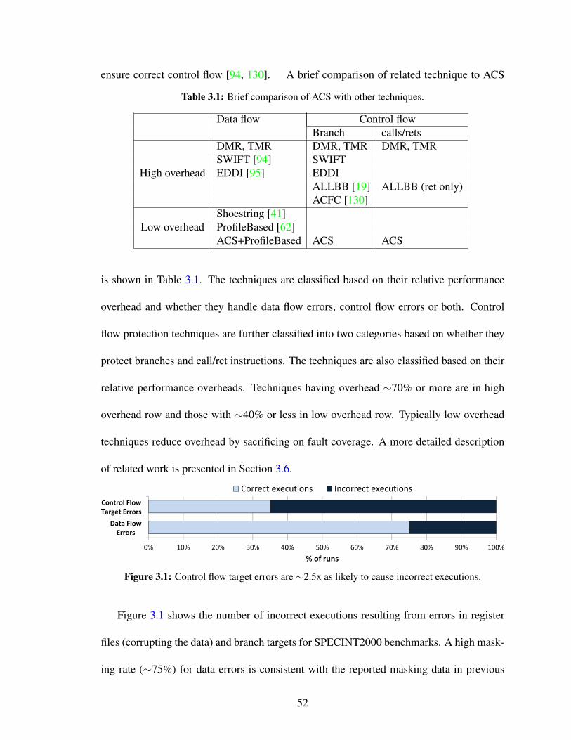
ensure correct control flow [94, 130]. A brief comparison of related technique to ACS
Table 3.1: Brief comparison of ACS with other techniques.
Data flow Control flowBranch calls/rets
High overhead
DMR, TMR DMR, TMR DMR, TMRSWIFT [94] SWIFTEDDI [95] EDDI
ALLBB [19] ALLBB (ret only)ACFC [130]
Low overheadShoestring [41]ProfileBased [62]ACS+ProfileBased ACS ACS
is shown in Table 3.1. The techniques are classified based on their relative performance
overhead and whether they handle data flow errors, control flow errors or both. Control
flow protection techniques are further classified into two categories based on whether they
protect branches and call/ret instructions. The techniques are also classified based on their
relative performance overheads. Techniques having overhead ∼70% or more are in high
overhead row and those with ∼40% or less in low overhead row. Typically low overhead
techniques reduce overhead by sacrificing on fault coverage. A more detailed description
of related work is presented in Section 3.6.
0% 10% 20% 30% 40% 50% 60% 70% 80% 90% 100%
Data Flow
Errors
Control Flow
Target Errors
% of runs
Correct executions Incorrect executions
Figure 3.1: Control flow target errors are ∼2.5x as likely to cause incorrect executions.
Figure 3.1 shows the number of incorrect executions resulting from errors in register
files (corrupting the data) and branch targets for SPECINT2000 benchmarks. A high mask-
ing rate (∼75%) for data errors is consistent with the reported masking data in previous
52

works [41, 133]. On average, errors in the branch targets are ∼2.5x more likely to result in
incorrect executions. Hence, in this chapter, we focus on efficient detection of control flow
errors, in branches as well as call/ret instructions, and our technique can be combined with
previously proposed [41, 62, 94] code duplication based solutions for a complete solution
(see Section 3.5.3 for a combined solution).
3.2.2 Control Flow Errors
Figure 3.2: Control Flow Target Errors: Corruption of branch target can result in nearby (Type A)or far away (Type B) displacement of control flow.
To better understand control flow protection techniques, we need to comprehend the
various cause of control flow errors. A control flow error can occur in a non-control flow
(e.g., add) or in a control flow (e.g., branch) instruction. A non-control flow instruction
of the application can be converted into a control flow instruction by a soft error thus
erroneously affecting control transfers. Errors occurring in control flow instructions can be
divided into two categories: Firstly, control flow condition errors are caused by the errors
in the direction of a conditional branch. Secondly, control flow target errors are caused
by the errors in the destination of a branch. Branch conditions are usually protected by data
53

flow protection schemes by duplicating the computation leading to a condition. As shown
later in Figure 3.10 (Section 3.4.3), the errors in branch targets result in disproportionately
high number of incorrect executions. Hence, we focus on the control flow disturbances
caused by the errors in branch targets. From here onwards, unless otherwise specified,
the use of control flow errors with respect to ACS refers to the errors in branch targets.
Figure 3.2 shows a part of a Control Flow Graph (CFG) containing 4 Basic Blocks (BBs).
Two types of errors that affect branch target are also shown in the Figure. Type A errors
cause the erroneous jump to nearby locations and Type B errors direct the control flow to
far away locations. Type A errors cause the program to skip a few instructions and are
more likely to result in masking or program output corruptions. In contrast, Type B errors
are more likely to crash the program either by directing the control flow to out of program
scope or to a different function in the same program. In Section 3.3, we describe how our
proposed method handles these control flow errors.
3.2.3 Signature Based Techniques and Associated Overheads
Figure 3.3: Basic signature scheme: If the correct control flow transfer takes place, G at dest_BBwould be equal to s2 otherwise not.
54

Many of the previously proposed software-only techniques for control flow protection
embed signatures or assertions into BBs at compile time [94, 45, 4]. This section briefly
describes the fundamentals of these signature based techniques, especially CFCSS [94].
CFCSS assigns a unique signature Si to each BB in the program. A general purpose register
(G) is used to hold the signature of the currently executing BB. G is initialized to the
signature of first BB when a program starts. Subsequently, whenever a transition is made
from src_BB to dest_BBs the value of G is updated with the newly computed value. This
new value is calculated by taking the xor of G and the static signature difference (xor) of
src_BB and dest_BB. After this, G should be equal to the unique signature assigned to
dest_BB. A comparison of G with unique value of dest_BB is inserted in dest_BB to
make sure that control flow is correct. If this comparison fails, an incorrect control flow
transfer has taken place. A simple case of this scheme is shown in Figure 3.3. For a
complex case of branch-fan-in nodes, extra dynamic adjusting signatures must be inserted
to avoid aliasing [94]. This necessitates the need for multiple signature updates in branch-
fan-in nodes and dynamic signature computation in predecessors BBs of the branch-fan-in
nodes. These extra updates contribute to the overhead of such a scheme.
Essentially, every BB in the application contains signature computation or update in-
structions as well as comparison instructions for ensuring correct control flow. The cost
of embedded signature checking at runtime in every BB can be prohibitive, making these
techniques impractical. We have implemented CFCSS and in our experiments on small
benchmarks (the same ones used in CFCSS [94]) we observe, on average, a performance
overhead of 68%. Though, for Insertsort benchmark from the set of benchmarks, it is as
high as 222%. For real representative benchmarks from SPECINT2000, we observe up to
55

a 144% overhead (75% on average) for the CFCSS technique. The opportunity to reduce
this huge overhead is one of the motivations behind proposing ACS.
3.3 Abstract Control Signatures
Figure 3.4: Abstract signatures: The whole program is divided into regions at a higher abstractionlevel. Such regions are enclosed by dashed light blue (grey) lines in this Figure. Every regionis assigned a signature. Every abstract region updates its signature based on the control transfersamong the BBs inside it. These signatures are only checked in other abstract regions.
Fundamentally, there are two critical aspects of any signature based control flow pro-
tection scheme. The first is signature computations (or updates) in each BB and the second
is signature comparisons (or checking) to check for erroneous control flow. These two
56

computations are the main contributors to the performance overhead of signature-based
control flow checking schemes. To reduce performance overhead, we propose raising the
level of abstraction of signature checking and simplifying signature updates in every BB.
The abstraction level is raised by working at the levels of regions∗. The whole program
is divided into regions that are larger than just a BB. These regions are more than just a
collection of BBs and ideally should possess certain properties that help in minimizing the
number of signature comparisons and signature updates. Each region has a signature vari-
able associated with it. For example, one desirable property of regions is to have a single
entry point so that the associated signature variable need not be initialized at every entry
point. As shown later (Section 3.3.2), this reduces the number of required signature com-
parisons. The signature variable associated with a region is checked in other regions that
are the target of the control flow edges from the region under consideration. Essentially,
signature information flows between these abstract regions. The signature associated with
each region represents the correctness of control flow internal to that region. In this sense,
checking control flow outside regions abstracts away the details about control flow inside a
region, hence the name ACS (Abstract Control Signatures). A high level diagram for ACS
concept is shown in Figure 3.4. In Figure 3.4 the signature sig1 is associated with region 1
and is updated inside the BBs of region 1. Assuming a BB in region 1 has a control flow
edge to a BB in region 3, sig1 would only be checked in that BB in region 3.
∗In this chapter, region is used to refer to a single entry multiple exit code section that satisfies thefollowing property among others: loop back edges are only allowed to the entry node (see Section 3.3.1).
57

3.3.1 Design of ACS
The idea of ACS is very generic and can be realized in various ways. ACS can be im-
plemented by forming regions at various granularity levels and different signature updates
according to the required trade-offs in performance overhead and fault coverage. The sig-
nature update inside each BB can also be tuned. For example, the signature update inside
each BB can be as simple as having a parity bit set/reset and the corresponding check would
be to check against 0 if even number of blocks were traversed and against 1 if odd number
of blocks were traversed. These updates can be more complex such as usage of hash func-
tions or xors. Similarly, the region formation can also be customized. For example, if the
region is a single BB then this scheme is the same as regular signature checking in each
BB.
For ACS implemented as a part of this chapter, we have made following choices for
signature updates and regions. We use a simple counter variable as the signature. For
signature updates, we increment the signature by 1 in the beginning of every BB. The
intuition behind using increment by 1 is as follows: Consider 2 points in a program, X is
a region entry and Y is the corresponding region exit. If control reaches X, we expect it
to reach Y. ÂaIf in going from X to Y, a valid number of BBs are traversed and the first
instruction in each of those BBs is executed, we hypothesize that control flow is likely
correct. ÂaObviously, this is not always true, but our experiments have confirmed that
small disruptions (fault in the lower bits of the branch target) in the control flow will result
in changes to the path length due to positioning of counter updates at the beginning of BBs
and large disruptions (fault in upper bits) will result in Y never being reached. ÂaThus,
58

if the hypothesis is statistically true, individual control transitions need not be checked
with minimal loss in fault coverage. This allows only the higher level information to need
checking. To see the usefulness of such counters, let us consider the control flow errors
shown in Figure 3.2. On one hand, Type B errors (far away erroneous jumps) that would
transfer control from one region to another, are easily caught. On the other hand, Type A
errors (nearby erroneous jumps) are likely to skip the signature updates, so they are also
caught. We use intervals [3] as regions because of the desirable properties they possess.
Intervals: An interval is a set of BBs such that every BB except the header BB in the
interval has its predecessors in the interval. An interval satisfies the following, and many
other, properties.
1. The header block of an interval dominates all the BBs in that interval. Basically, this
implies that control can only enter at the header node of an interval.
2. If a loop is part of an interval then the loop header and interval header are the same.
The header BB of a loop is the target BB of back edges in that loop.
Figure 3.5 shows an example of intervals for a CFG that has nested loops. Interval 1
contains only bb1 and its header is also bb1. Interval 2 contains all the remaining blocks
shown in the Figure. Interval 2 contains a loop and note that loop header bb2 is also the
header node of the interval 2. Another interesting observation is that the outer loop is never
contained in a single interval. We use intervals formed according to the maximal interval
definition [88]. A latch BB of a loop is defined as the block that has a branch to the header
of the loop. For example, bb_latch1 is the latch block for the inner loop starting at bb2.
A basic overview of the implemented scheme is shown in Figure 3.6. The counter C1
59
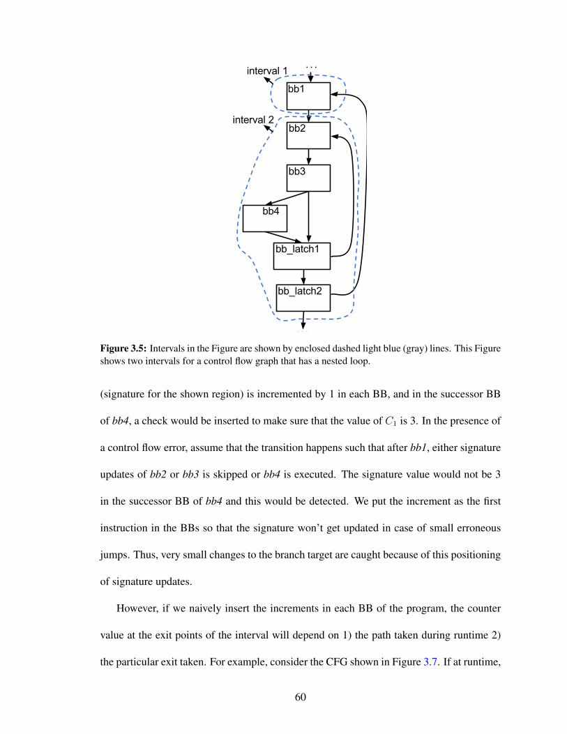
Figure 3.5: Intervals in the Figure are shown by enclosed dashed light blue (gray) lines. This Figureshows two intervals for a control flow graph that has a nested loop.
(signature for the shown region) is incremented by 1 in each BB, and in the successor BB
of bb4, a check would be inserted to make sure that the value of C1 is 3. In the presence of
a control flow error, assume that the transition happens such that after bb1, either signature
updates of bb2 or bb3 is skipped or bb4 is executed. The signature value would not be 3
in the successor BB of bb4 and this would be detected. We put the increment as the first
instruction in the BBs so that the signature won’t get updated in case of small erroneous
jumps. Thus, very small changes to the branch target are caught because of this positioning
of signature updates.
However, if we naively insert the increments in each BB of the program, the counter
value at the exit points of the interval will depend on 1) the path taken during runtime 2)
the particular exit taken. For example, consider the CFG shown in Figure 3.7. If at runtime,
60

Figure 3.6: Every interval is associated with a signature. In our scheme, signature are simplecounters. The signature is initialized in the header and incremented by 1 in other blocks. Thesignature checks are made in the BBs that are destination BBs of exits out of an interval.
edge bb1 → bb2 is traversed, the signature value at the exit out of bb3 would be 3 since
each BB increments signature by 1. However, if the edge bb1→ bb3 is traversed signature
value at the same point would be 2. Another similar problem exists if there are multiple
exit points from an interval. The signature values at the exit points of an interval would
be different if the exits originate from different BBs. Different signature values from an
interval exit would imply that checks would need to be inserted with different values. To
solve this problem, we make sure that from every exit out of an interval, the same signature
value needs to be checked no matter which exit is taken. To tackle the aforementioned
problems, we have developed a method to calculate extra balancing increments required
along edges. The details of this method are described in the next subsection.
61
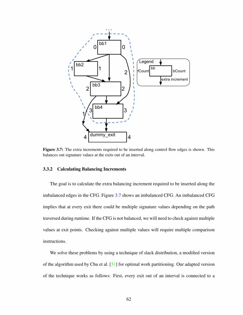
Figure 3.7: The extra increments required to be inserted along control flow edges is shown. Thisbalances out signature values at the exits out of an interval.
3.3.2 Calculating Balancing Increments
The goal is to calculate the extra balancing increment required to be inserted along the
imbalanced edges in the CFG. Figure 3.7 shows an imbalanced CFG. An imbalanced CFG
implies that at every exit there could be multiple signature values depending on the path
traversed during runtime. If the CFG is not balanced, we will need to check against multiple
values at exit points. Checking against multiple values will require multiple comparison
instructions.
We solve these problems by using a technique of slack distribution, a modified version
of the algorithm used by Chu et al. [31] for optimal work partitioning. Our adapted version
of the technique works as follows: First, every exit out of an interval is connected to a
62
dummy exit node. All BBs in the interval are assigned a fCount of 0. All edgeWeights
are initialized to 1 and represent an initial increment along the associated edge. fCount
is a number associated with each BB that represents the path length from the header of
an interval to the BB under consideration. The algorithm starts from the header BB of
the interval. By iterating over predecessors, the sum of edgeWeight and fCount for each
predecessor is calculated. fCount for the current block is then maximum value over all pre-
decessors. This can be written as follows: fCount(bb) = maxx∈predecessors(bb)(fCount(x) +
edgeWeight(x → bb)). For every interval, this calculation is repeated until there is no
change in fCount value of any BB. The pseudo code of the algorithm is described in Algo-
rithm 1. Every BB is also associated with a number called bCount . bCount is the number
calculated starting from dummy exit nodes and traversing the predecessors. bCount are
initialized to fCount for each BB. Using an algorithm similar to the one shown in Algo-
rithm 1, bCount is calculated for every BB in the interval. The update equation of bCount
is as follows: bCount(bb) = minx∈successors(bb)(bCount(x)− edgeWeight(x→ bb)). Note
that during the calculation of fCount and bCount only the successors and predecessors that
are in the interval are considered. The dummy_exit block is considered a part of the inter-
val during analysis. Once the fCount and bCount calculation is completed for every BB in
the interval, the amount of extra balancing increment to be inserted along an edge between
srcBB and destBB can be calculated as follows: extraIncrement [srcBB → destBB ] =
fCount [destBB ]− edgeWeight [srcBB → destBB ]− bCount [srcBB ].
Figure 3.7 shows an example of extra increment calculation for a CFG. Numbers on the
left side of blocks represent fCount and numbers on right side of the BB represent bCount .
Numbers on the edges are the extra increments required to be inserted along that edge. e.g.,
63

based on the algorithm described above edge bb1 → bb3 edge gets an increment of 1
and edge bb1 → bb4 gets an increment of 2. Once this step is executed, all the required
increments are inserted along all edges of an interval.
Create dummy_exit block and connect all exit edges to this block;Initialize all edgeWeight to one;Initialize all fCount to zero;change = 1;while change do
change = 0;for each bb in Interval do
maximum = max(fCount(x) + edgeWeight(x→ bb)) for x inpredecessors[bb] and x→ bb is not a backEdge;if fCount[bb] < maximum then
change = 1;fCount[bb] = maximum;
endend
endAlgorithm 1: Algorithm for calculating fCount for every BB in an interval.
3.3.3 Error Detection Analysis
Let Ci be the counter associated with an interval. Every block inside that interval
updates the counter by 1 and at every exit out of the interval the counter value should
be the maximum path length (since we insert balancing increments) through that interval.
Let that max value for an interval be CMax . If Ci is not equal to CMax when control
exits out of the interval then the control flow inside the program got disturbed. For all the
intra-interval control flow errors, if any update to the path length counter is skipped, the
path length calculation would be wrong and hence the control flow error will get caught.
Erroneous jumps to other intervals are detected as the path length is not correct at the entry
point of those intervals. However, there could be multiple paths of same length inside
64
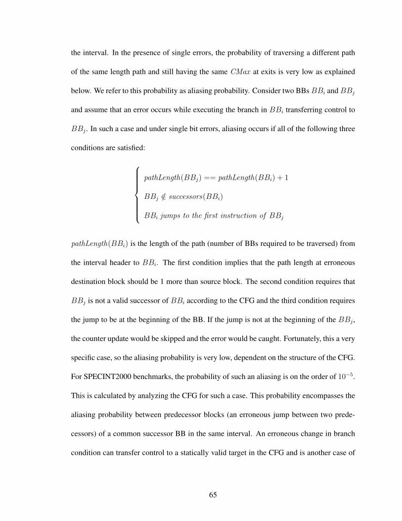
the interval. In the presence of single errors, the probability of traversing a different path
of the same length path and still having the same CMax at exits is very low as explained
below. We refer to this probability as aliasing probability. Consider two BBsBBi andBBj
and assume that an error occurs while executing the branch in BBi transferring control to
BBj . In such a case and under single bit errors, aliasing occurs if all of the following three
conditions are satisfied:
pathLength(BBj) == pathLength(BBi) + 1
BBj /∈ successors(BBi)
BBi jumps to the first instruction of BBj
pathLength(BBi) is the length of the path (number of BBs required to be traversed) from
the interval header to BBi. The first condition implies that the path length at erroneous
destination block should be 1 more than source block. The second condition requires that
BBj is not a valid successor of BBi according to the CFG and the third condition requires
the jump to be at the beginning of the BB. If the jump is not at the beginning of the BBj ,
the counter update would be skipped and the error would be caught. Fortunately, this a very
specific case, so the aliasing probability is very low, dependent on the structure of the CFG.
For SPECINT2000 benchmarks, the probability of such an aliasing is on the order of 10−5.
This is calculated by analyzing the CFG for such a case. This probability encompasses the
aliasing probability between predecessor blocks (an erroneous jump between two prede-
cessors) of a common successor BB in the same interval. An erroneous change in branch
condition can transfer control to a statically valid target in the CFG and is another case of
65

aliasing. We assume that such a case can be handled by data flow protection methods.
3.3.4 Insertion of Checking Instructions
An important part of the technique is to find the BBs where the comparison instructions
should be inserted. Each interval has a unique signature variable. We compare this variable
with the statically known CMax to test that the proper number of increments occurred. For
our initial implementation, we chose to insert checks at all the exit points of an interval and
in the latch block of loops. However, this is suboptimal and in the next section we show
that how this can be further optimized.
3.3.5 Optimization for Loops
(a) Checks for loops (b) Optimized insertion of checking instruc-tion
Figure 3.8: Optimizing signature checking for loops: The checks on signatures are moved out ofloops to exit blocks so that they are not executed in each iteration.
66

A naive way to insert a checking instruction for a loop is as shown in Figure 3.8(a).
The latch block contains the checking instruction (the instruction that compares C1 to 3).
However, in this situation, the check is executed once every loop iteration. This can be
optimized as shown in Figure 3.8(b). In the optimized case, the checking instruction is
moved out of the loop and check is now made against a remainder. Essentially, a multiple
of loop path length gets tested by the remainder. Remainders are a costly operation and
one important issue to consider here is the fact that loop increments are inserted in such a
way that the remainder is always taken by a power of two. This is shown in Figure 3.8(b),
in bb4 counter C1 is incremented by 2 instead of 1 to make sure that remainder by 4 is
taken. If this is the case the remainder instruction can simply be converted to a bitwise and
instruction (e.g., remainder by 4 can be computed as bitwise and with 3).
3.3.6 Call and Return Instructions
A source of control flow transfers are call and return instructions. In this chapter, we
propose a new technique to protect the control flow from caller to callee header and the
return from callee to caller. The idea is akin to the path length approach used for branches
except each function call has a unique path length (a unique number) that is checked upon
entry of the callee and upon return to the caller to ensure call/returns go to and return from
proper targets. We make the path length unique for each function to ensure that there is no
aliasing among calls to different functions. The technique works as follows: Let F be the
set of all the functions in an application. Every fi ∈ F is assigned a unique code such a
67

way that the following is true.
HammingDistance(ACode(fi), ACode(fj)) > 1
∀fi, fj ∈ F and i 6= j
For binary numbers a and b, Hamming distance is equal to the number of positions at which
the corresponding bits in a and b are different. Simply put, Hamming distance is the num-
ber of errors required to transform a to b, and vice versa. HammingDistance(a, b) is the
Hamming distance between a and b. ACode(fi) represents the code assigned to fi. Every
function in the application is assigned a unique code in a way such that the Hamming dis-
tance between any two codes is greater than 1. This ensures that there is no aliasing among
calls because of erroneous transition from one function to another function in presence of
single bit errors. Figure 3.9 shows an example of instrumented code. The Global Signa-
Figure 3.9: Handling call and return instructions. Instructions in bold represent the inserted in-structions.
ture Register (GSR) is updated before and after the call as shown. RConst is a convenient
constant (power of 2) chosen in a way such that the costly remainder operation can be con-
verted to simple bit shift operation. 34 is the Hamming code assigned to the function Foo.
68

Inside the callee, the GSR is updated in the entry BB of the callee and return BB of the
callee. This ensures that other calls inside Foo can use the same type of instrumentation.
If source code of a call (e.g., library calls) is not available then the increments inside the
callee cannot be inserted and only the increments around the call are inserted. In such a
case, the transition to the beginning of the callee cannot be checked but the instrumented
code ensures the return from callee should be right after the call instruction. Calls through
pointers and compiler built-ins (i.e., compiler intrinsics) are treated in the same way as
library calls.
3.4 Experimental Setup
A common practice in the literature to evaluate transient fault detection solutions is to
use Statistical Fault Injections (SFIs) into a microarchitectural model of a processor. We
believe that SFI provides the opportunity to inject faults into various hardware structures
and hence are close to real transient fault scenarios. SFI has been previously [41, 101] used
in validating the solutions proposed to protect against soft errors.
3.4.1 Compiler Transformations
We have used the LLVM [66] compiler infrastructure to insert ACS into an application’s
code. Firstly, application source code is converted into LLVM’s internal representation
called LLVM IR (Intermediate Representation). ACS is implemented as a pass over LLVM
IR. ACS insertion pass should be run after all the optimization passes on IR so that these
passes do not interfere with ACS code. Our ACS insertion pass takes IR as input and
69

as output it generates IR with signature computations and checks embedded into it. An
LLVM interval formation pass is internally run and the information is used to insert control
flow checking signatures. Some optimization passes such as constant propagation in code
generation phase can propagate the constant initialization of signatures into the next BB.
This can effectively remove the effect of inserted signature from the BB where the signature
was initialized to its successors BBs. We have disabled such optimizations during the phase
when LLVM prepares the IR for code generation.
3.4.2 Benchmarks
We have used 11 benchmarks from the SPECINT2000 benchmark suite (gzip, vpr, gcc,
mcf, crafty, perlbmk, parser, gap, vortex, bzip2, twolf) as representative workloads in exper-
iments. All these benchmarks were compiled with -O3 option of gcc frontend for LLVM.
SPECINT2000 benchmarks. In the context of embedded systems, if the change in execu-
tion time affects program output, these programs might not run correctly after control flow
protection. We do not consider multithreaded benchmarks in this chapter. However, we do
not foresee any problems of using ACS with multithreaded programs.
3.4.3 Fault Injection Campaign
To evaluate the proposed approach, we ran an extensive fault injection campaign. An
acceptable way in literature to model transient faults is using single bit-flips. These faults
are inserted by flipping a random bit at a random cycle during the course of the applica-
tion run. We injected faults in the register file (a large part of the processor’s architectural
state) and branch targets. A fault in a register used as branch target or in the computation
70

0%
10%
20%
30%
40%
50%
60%
70%
80%
90%
100%
Inco
rre
ct e
xe
cuti
on
s ca
use
d
by
co
ntr
ol
flo
w f
au
tls
Figure 3.10: The incorrect executions as a percentage of unmasked faults caused by disturbance incontrol flow targets. Faults are injected in register file as well as branch targets.
of branch targets for indirect branches can disturb the control flow. Figure 3.10 shows the
results of this experiment and Y-axis in the Figure is incorrect executions caused by control
flow target errors as a percentage of the unmasked faults. The results show that a large
percentage (on average 42%) of the unmasked faults result in incorrect executions and are
caused by control flow faults. 175.vpr and 300.twolf (100% bars in the Figure 3.10) have
high masking rate and all the remaining incorrect executions for these two benchmarks are
caused by control flow faults. Even though the size of branch target (32 bit) is smaller
than register file (16 registers of size 32 each), the contribution of branch target errors to
incorrect executions is disproportionately high. Hence, control flow faults are an important
category of faults to consider. Therefore, for the rest of the experiments, we chose to inject
faults in branch targets only. Injecting faults in branch targets represents stress testing (a
pessimistic case) control flow protection schemes since all the injected faults are guaran-
teed to disturb the control flow and subsequently do not inflate coverage numbers as they
71

result in less masking compared to data errors as shown in Figure 3.1. The same method
of fault injection is used for the baseline (CFCSS). To inject a fault, the program runs nor-
mally until it encounters the first control flow instruction after the selected random point is
encountered. Once the control flow instruction is selected, a random bit is selected from the
target address of the control flow instruction. This selected random bit is flipped to com-
plete the injection of fault. Faults in PC (Program Counter) and other address circuitry are
expected to disturb the control flow in a similar manner. Our technique is also capable of
detecting faults injected into other microarchitectural units that affect the program control
flow.
We used the GEM5 [16] simulator to simulate the workloads and implemented fault
injection infrastructure into this simulator. The simulator was run in ARM syscall emula-
tion mode and modeled the ARMv7-a profile of ARM architecture. To obtain performance
overhead, workloads are simulated in an out-of-order model of the target processor. We use
atomic model for processor configuration to inject control flow faults. The details of the
processor configuration for out-of-order model used for the experiments are in Table 3.2.
Table 3.2: GEM5 Simulator parameters (models an ARMv7-a profile of ARM architecture).
Processor core @ 2GHzSimulation configuration out-of-order coreSimulation mode Syscall emulationPhysical integer register file size 256 entriesReorder Buffer Size 192 entriesIssue width 2
MemoryL1-D cache 64KB, 2-wayL1-I cache 32KB, 2-wayDTLB/ITLB 64 entries (each)
We have chosen to inject 1100 faults per technique to evaluate the solution. The statis-
72

tical significance of these faults can be calculated by leveraging the work done by Leveugle
et al. [69]. The calculation for our experimental setup shows that we need 96 fault injec-
tion trials for each benchmark to have a 10% margin of error and confidence level of 95%.
Note that the margin of error only applies to fault coverage data. The performance over-
head shows the exact simulation cycles consumed by the simulator. Therefore, we chose
100 fault injection trials for each benchmark to yield results with reasonable accuracy in a
timely manner. After the fault injection, the program runs until completion. The result of
each simulation trial is classified into one of the following five categories:
• Masked: The injected fault did not corrupt the program output. Application-level or
architecture-level masking occurred in this case.
• HWDetect: The injected fault produces a symptom such as a page fault so that
a recovery can be triggered. A fault is considered under this category only if the
symptom is produced within a number of cycles (2000 for our experiments) after the
fault was injected.
• CFDetect: The injected fault was detected by the control flow checking instructions
inserted at the time of compiler transformation.
• Failure: The injected fault resulted in out-of-bound address access and resulted in
simulation termination. Also, faults causing infinite loops in the program are classi-
fied under this category.
• SDC: Faults that corrupt the program output are classified into this category. These
are Silent Data Corruptions.
73

Traditionally, the fault tolerance research community considers a program to be cor-
rect if the architectural state is correct at every cycle. Li et al. [73] showed that 17.6%
of the multimedia and AI applications showed correct results even though they had archi-
tecturally incorrect states. We believe that user-visible program output corruptions truly
matter to end users and cycle-by-cycle correct architectural state is not important to them.
So in the context of evaluating this work, a program is considered to have executed cor-
rectly if the final output of the program matches. The result classifications of the injection
experiments in this chapter are based on the fact that only program output corruptions really
matter. Therefore, for this work we do not regard the number of faults that propagate to the
microarchitectural state as a metric of importance. The percentage of faults that actually do
corrupt program output are considered harmful because these faults corrupt program output
without any hint of failure and represent the worse case scenario.
3.4.4 Recovery Support
ACS, like CFCSS, is a detection-only solution for control flow errors. Once a control
flow error is detected, we rely on a recovery mechanism to recover from the detected error.
A software-only recovery scheme such as Encore [42] or checkpointing-based recovery
schemes can be used in conjunction with our solution. Feng et al. [41] and Wang et al. [132]
proposed that future microprocessors with aggressive performance speculation will need
recovery support. If available, the same scheme can be used by our solution. However,
the cost of checkpointing-based and software-only schemes increases with respect to the
number of instructions executed from recovery point. So, one important target for our
scheme is to keep a bound on fault detection latency.
74

0%
20%
40%
60%
80%
100%
120%
140%
160%
Pe
rfo
rma
nce
Ov
erh
ea
d (
run
tim
e)
CFCSS CFCSS_ivl ACS_w/o_calls_rets ACS_w/_calls_rets
Figure 3.11: The performance (Runtime on simulated core) overhead for all techniques.
3.5 Experimental Evaluation and Analysis
Using the experimental setup described in Section 3.4, we obtain performance overhead
and fault coverage results. Figure 3.11 shows the performance overhead measured in terms
of runtime. These overheads are in comparison to unmodified applications compiled at
-O3 optimization level. CFCSS shows the runtime overhead for the CFCSS scheme [94]
and CFCSS_ivl bar shows the instruction overhead if the interval information is used in
conjunction with CFCSS to insert checking at a coarser granularity. CFCSS_ivl has the
xor (same as CFCSS) signature update inside every BB and in contrast to CFCSS only
signature checking is moved at a coarser granularity. Also, CFCSS_ivl does not have any
loop optimizations (Section 3.3.5). The third and fourth bar for each benchmarks shows
the runtime overhead when we use ACS. ACS_w/o_calls_rets bar in this Figure shows the
overhead without the protection for calls and returns (Section 3.3.6) and ACS_w/_calls_rets
the overhead if protection for calls and rets is included. Overall, the performance overhead
75

0%
10%
20%
30%
40%
50%
60%
70%
80%
90%
100%
CFCSS
CFCSS_ivl
ACS_w/o_calls_rets
ACS_w/_calls_rets
CFCSS
CFCSS_ivl
ACS_w/o_calls_rets
ACS_w/_calls_rets
CFCSS
CFCSS_ivl
ACS_w/o_calls_rets
ACS_w/_calls_rets
CFCSS
CFCSS_ivl
ACS_w/o_calls_rets
ACS_w/_calls_rets
CFCSS
CFCSS_ivl
ACS_w/o_calls_rets
ACS_w/_calls_rets
CFCSS
CFCSS_ivl
ACS_w/o_calls_rets
ACS_w/_calls_rets
CFCSS
CFCSS_ivl
ACS_w/o_calls_rets
ACS_w/_calls_rets
CFCSS
CFCSS_ivl
ACS_w/o_calls_rets
ACS_w/_calls_rets
CFCSS
CFCSS_ivl
ACS_w/o_calls_rets
ACS_w/_calls_rets
CFCSS
CFCSS_ivl
ACS_w/o_calls_rets
ACS_w/_calls_rets
CFCSS
CFCSS_ivl
ACS_w/o_calls_rets
ACS_w/_calls_rets
CFCSS
CFCSS_ivl
ACS_w/o_calls_rets
ACS_w/_calls_rets
164.gzip 175.vpr 176.gcc 181.mcf 186.crafty 197.parser 253.perl 254.gap 255.vortex 256.bzip2 300.twolf average
% o
f ru
ns
Masked CFDetects HWDetects Failures SDCs
Figure 3.12: CFCSS bar shows the fault coverage for CFCSS and CFCSS_ivl shows the faultcoverage with checking inserted using interval information. ACS_w/o_calls_rets shows the faultcoverage without protection for calls/returns and ACS_w/o_calls_rets shows the fault coverage ifcalls/returns are also protected.
is 75%, 57.8%, 11% and 28.8% for CFCSS, CFCSS_ivl, ACS_w/o_calls_rets and ACS_-
w/_calls_rets, respectively. We have also measured the impact of code size expansion
on application binaries and on average code size overhead is 22% with ACS. The code
size overhead is largest for 176.gcc showing largest performance overhead. To give more
insight on the reduction in overhead, we measured the number of intervals and basic blocks
in benchmarks. On average, there are 13302 basic blocks and 1993 intervals across the
evaluated benchmarks and the number of checks required to be inserted are 2461. This
represents a 5.4x decrease in the number of checks by abstracting from BBs to intervals.
In the next experiment, we explore the fault coverage provided by these techniques.
We define fault coverage as the percentage of faults out of total injected faults that do not
result in Silent Data Corruptions (SDCs). SDCs are the most harmful errors because the
program silently corrupts data while the user thinks that application worked as expected.
The faults classified in HWDetects imply that these symptoms can be used to trigger re-
covery [41, 132]. Each bar in Figure 3.12 shows the distribution of faults among different
categories when the instrumented application runs with fault injections. The four bars are
76

0.90
0.95
1.00
1.05
1.10
1.15
1.20
1.25
CFCSS
ACS
CFCSS
ACS
CFCSS
ACS
CFCSS
ACS
CFCSS
ACS
CFCSS
ACS
CFCSS
ACS
CFCSS
ACS
CFCSS
ACS
CFCSS
ACS
CFCSS
ACS
CFCSS
ACS
164.gzip 175.vpr 176.gcc 181.mcf 186.crafty197.parser 253.perl 254.gap 255.vortex256.bzip2 300.twolf avg
No
rma
lize
d d
ete
ctio
n l
ate
ncy
WithIn2K WithIn5K Within10K WithIn100K
Figure 3.13: Comparison of fault detection latency with CFCSS. The fault detection latency is notadversely affected.
the fault distribution for CFCSS, CFCSS_ivl, ACS_w/o_calls_rets and ACS_w/_calls_rets
and the average fault coverage for these techniques is 98.8%, 98.4%, 96.6% and 96.3%, re-
spectively. All these techniques reduce the number of SDCs in comparison to unprotected
application, but ACS without calls/rets protection has only 11% performance overhead in
comparison to 75% performance overhead of CFCSS.
3.5.1 Fault Detection Latency
Another important metric with regard to fault detection techniques is the detection la-
tency. Fault detection latency is directly related to the overhead of a recovery scheme. A
longer latency implies that either the fault cannot be recovered or the recovery overhead
would be high. Figure 3.13 shows the latency of ACS with respect to CFCSS. WithIn2K
represents the number of faults detected in less than 2000 (2K) cycles of injections. Simi-
larly, WithIn5K, WithIn10K and WithIn100K represents the number of fault detected within
77

5000, 10000 and 100000 cycles of injection, respectively. These categories are cumulative
and faults classified under WithIn5K include all the faults detected with in 5K cycles, i.e., it
subsumes the faults classified under WithIn2K. Similar rules apply for faults detected with
in 10K and 100K cycles. The bars in the figure are normalized with respect to the number
of faults detected in WithIn2K. For example, the WithIn5K bars represent the ratio of the
number of faults detected with in 5K cycles and number of faults detected with in 2K cy-
cles. In case of ACS, on average, WithIn5K contains 2% more than WithIn2K. Similarly,
WithIn10K and WithIn100K contain only 3% and 5% more faults than WithIn2K. The same
numbers for CFCSS are 0%, 1% and 1% for 5K, 10K and 100K cycles, respectively. Over-
all, ACS only increases the detection latency for at most 5% of the faults detected within
2K cycles.
3.5.2 Analysis of SDCs
In this subsection, we discuss some of the cases that escape the detection by CFCSS
and ACS control flow methods and eventually result in silent data corruptions. LLVM
IR supports the switch statements as the terminating instruction of BBs. When the code
generation phase converts this switch statement to machine instructions, it is converted
into multiple branches. Since these branches were not visible to our code instrumentation
pass, these do not get protected by ACS or CFCSS. Some of the faults that affect such
unprotected branches eventually cause SDCs. One way to handle these switch statements
is to convert all the switch statements to if-else in the LLVM IR itself before running our
code instrumentation pass. Another frequent case of SDCs is the faults that displace target
address (i.e., faults in low order bits) only by few instructions usually result in SDCs. For
78

example, we noticed that a fault in second bit of target address of a back edge caused
only two extra instructions to be executed. Those two extra instructions happened to be
immediate mov instructions and they just disturbed the value of two registers. Affected
registers were written to memory and hence caused SDC. A similar problem also exists
with CFCSS.
3.5.3 Data and Control Flow Protection
In this subsection, we present the results for combining a profile-based data flow [62]
and our proposed control flow solution. Figure 3.14 shows the performance overhead on
the primary vertical axis and fault coverage on the secondary vertical axis when a com-
bination of ACS and profile based data flow protection is used. SWDetects category in
the fault outcome classification represents the number of faults detected by software (both
data and control flow) and other category are same as previously mentioned. Control flow
condition errors are handled by duplicating the computations for branch conditions. A
combined solution incurs an average performance overhead of 47.4% and provides 96.5%
fault coverage. The binary is 35% larger and overhead on dynamic instructions is 55.4%.
SWIFT [101] is another solution that used data duplication. By leveraging the ideas from
CFCSS, SWIFT also enhances control flow protection. In comparison to ACS with data
duplication, SWIFT incurs an increase of: 2.3x for dynamic instructions, 2.3x for binary
size and 1.53x for execution time over the same set of benchmarks as used in this work
even though the performance overhead of SWIFT was measured on a aggressive server
class workstation targeting a different ISA (IA64) than our evaluations (ARM). An IA64
system can take better advantage of instruction level parallelism introduced by duplication
79

0%
10%
20%
30%
40%
50%
60%
70%
80%
90%
100%
0
10
20
30
40
50
60
70
80
90
100
% o
f ru
ns
% P
erfo
rm
an
ce
Ov
ere
ha
d
Overhead (Data flow) Overhead (Contorl flow) Masked SWDetects HWDetects Failures SDCs
Figure 3.14: Performance overhead and fault coverage for complete data and control flow protec-tion.
of instructions.
3.5.4 Discussion and Limitations
Similar to other signature based schemes [94, 4], ACS cannot detect faults in branch
conditions. Though other schemes [127, 45] can detect errors in a branch condition if the
error occurs after the branch condition is evaluated. This still misses the errors happening
before condition evaluation and in variables used in evaluation of that condition. Corrupt
branch conditions or other variables used to compute branch conditions can cause control
flow condition errors. These errors in branch conditions can be handled by combining ACS
with data flow protection based methods as described in Section 3.5.3. In this chapter, we
focus on the faults in branch targets and other variables used in computing branch targets.
In the presence of an error in the inserted checking code, the following scenarios can
occur: 1) If the check evaluates to True, then the error in signature comparison branch
80

will result in skipping the signature updates of next basic block, hence the error will be
caught at the next check. 2) If the check is wrong (i.e., an error has already occurred), then
considering that a transient fault is a rare event, a second error in this short span of time in
signature comparison is probabilistically unlikely to occur.
In LLVM, the CFG is the basis of data flow analysis and many optimizations. To
facilitate this data flow analysis, LLVM doesn’t allow the address of a BB to be taken and
then jump to it. Jumps to a location specified in a variable can only exist in the form of
call instructions and for other control flow instructions target BBs are known at LLVM IR
level. So at LLVM IR level, there is no special handling for indirect branches is required.
3.6 Related Work
Control flow protection is becoming an increasingly important concern for reliability
researchers. Two particularly noteworthy pieces of software-only work in this area are
CFCSS [94] and ECCA (Enhanced Control Flow Checking using Assertions) [4]. In our
experimental results, we have compared our work with CFCSS in detail. ECCA assigns a
unique prime identifier to each BB in the program and checks prime identifier at runtime
using an assertion in every BB. The authors of [130] reported that ECCA incurs 150%
memory overhead. Venkatasubramanian et.al [130] use parity in each BB to check for
correct control flow. Control flow is checked by special variables inserted in each routine.
The main difference with respect to these techniques and ACS lies in the fact that we raise
the level of abstraction for checking and the signature update is simplified in each BB. Borin
et al. [19] presented a control flow error detection technique where the signature checks are
81

made in 1) every BB, 2) only in the BBs with back edges and BBs with return instructions,
3) only in BBs with return instructions and 4) only at the end of the application. This
previous work reports 77% overhead for the case 1 and 37% for the case 3, in comparison to
11% overhead of ACS. Fault coverage data or detection latency for these different checking
granularity is not reported in the paper. It is expected that delaying the checking to loop end
points (blocks with back edges) and function ends (return blocks) will result in relatively
more failures and program corruptions or will affect detection time. CEDA [127] is an
assertion based scheme that assigns static signatures while minimize aliasing. The overhead
of CEDA for common benchmarks is 27.1% in comparison to 11% of ACS. CEDA work
also presents comparison with CFCSS and YACCA [45]. The performance overhead of
CEDA reported in that paper is comparable to CFCSS for the chosen five benchmarks with
a slightly better fault coverage. Since ACS has lower overhead than CFCSS, it will also
have lower overhead than CEDA. The paper reports YACCA’s overhead even larger than
that of CFCSS and CEDA.
A comparison with SWIFT [101] is already described in Section 3.5.3. Other works
such as CRAFT and PROFIT [102] improve upon the SWIFT solution by using additional
hardware structures and architectural vulnerability factor (AVF) analysis [92]. Our goal in
this work is to make the control flow protection practical for commodity embedded systems
by reducing the performance overhead. Our experimental results demonstrate that this
can be achieved at significantly less performance overhead than these previously proposed
techniques.
Symptom detection based solutions rely on anomalous microarchitectural behavior to
detect soft errors. A light-weight approach for detecting soft errors, ReStore [132], an-
82

alyzes symptoms including memory exceptions, branch mispredicts, and cache misses.
mSWAT [76] presented a solution which detects anomalous software behavior to provide a
reliable system. It requires special simple hardware detectors to detect faults. These tech-
niques are orthogonal to ACS, as they rely on specialized hardware. If available, they can
be leveraged along with ACS to increase the number of faults detected under HWDetects
category.
A category of previous works related to control flow protection are watchdog processor
based solutions [77]. The general idea of these techniques is to have a watchdog processor,
along side the main processor, that monitors and checks the program executing on the main
processor. These solutions rely on the availability of watchdog processor and in some
cases even propose specific changes to the watchdog processors. A variety of watchdog
based solutions [127, 82, 75] are proposed in literature by modifying some aspect (e.g.,
changing the type of signatures) of the technique. Some recent solutions also suggest the
idea of distributed checking in the core for various components. Argus [81], for example,
relies on a series of hardware checker units to perform online invariant checking to ensure
correct application execution (data flow as well as control flow). Argus achieves very low
overhead by adding extra hardware. In comparison to these techniques, ACS targets COTS
components and does not require any hardware changes.
An interesting approach to soft error reliability is using Redundant Multithreading
(RMT). AR-SMT [108] introduced the idea of RMT on SMT cores; The work is done by a
leading thread, and the trailing thread checks for the correctness. Subsequent works [100,
46] in this category have tried to reduce the overhead due to RMT. All these techniques
come with the overhead of running an extra thread which executes a skeleton of the origi-
83

nal program.
Another compiler assisted solution for control flow checking uses extra hardware to
minimize the overhead [71]. It requires compiler, as well as hardware changes. Ours is a
software-only approach to produce protected programs.
There is a large body of related work in Control Flow Integrity (CFI) [1] for com-
puter security against external software attacks. CFI works by making sure that all the
control transfer occur as determined by the static CFG. The failure model targeted by CFI
schemes is very different from soft errors failure mode. In CFI, constant destinations (di-
rect branches ) are statically verified and while computed (dynamic branches) are verified
for correct destination by instrumenting the code. Soft errors can affect the direct as well
as indirect branches and hence CFI, as is, is not directly applicable for soft errors. Though
direct branches can also be protected in a manner similar to dynamic branches, but the
already high overhead (20%-60% for dynamic branches only) would become prohibitive.
Path profiling [11] finds the execution count of a path in a Directed Acyclic Graph
(DAG). It is a related problem to our work and gives an unique number for each path in a
DAG. However, we want to have a balanced path length along with information about edges
in the path to insert balancing increments. This can not be obtained with path profiling.
Moreover, usually profiling is created with training inputs but later the program might be
executed with a different set of inputs. In ACS, we need the correct path length with the
current inputs a program is executing. Therefore, the data produced by off-line profiling
can not be used in ACS.
84

3.7 Conclusions
The ever increasing desire to create powerful and efficient microprocessors, with each
successive new generation, has led to the use of increasingly smaller transistors into these
devices. Aggressive scaling makes transistor devices more susceptible to transient faults.
To tackle the problem of control flow protection at minimal performance overhead, we have
proposed Abstract Control flow Signatures (ACS). ACS achieves its efficiency by working
at a coarse-grain level than the previously proposed signature based techniques and also by
simplifying signature updates in each basic block. ACS reduces performance overhead, on
average, from 75% down to 11% while maintaining the similar level of fault coverage in
comparison to a previously proposed approach (CFCSS [94]).
85

CHAPTER IV
Harnessing Soft Computations for Low-budget Fault
Tolerance
A growing number of applications from various domains such as multimedia, machine
learning, and computer vision are inherently fault tolerant. However, for these soft work-
loads, not all computations are fault tolerant (e.g., a loop trip count). In this chapter, we
propose a compiler-based approach that takes advantage of soft computations inherent in
the aforementioned class of workloads to bring down the cost of software-only transient
fault detection. The technique works by identifying a small subset of critical variables that
are necessary for correct macro-operation of the program. Traditional duplication and com-
parison is used to protect these variables. For the remaining variables and temporaries that
only affect the micro-operation of the program, strategic expected value checks are inserted
into the code. Intuitively, a computation-chain result near the expected value is either cor-
rect or close enough to the correct result so that it does not matter for non-critical variables.
The overall goal here is to minimize the number of user unacceptable output corruptions.
Exact output is not necessary in the aforementioned classes of applications if an user can
86
tolerate approximate outputs.
4.1 Introduction
An increasing number of both current and emerging workloads from domains such as
multimedia, machine learning, computer vision, etc., either compute on approximate data
and/or produce results that have subjective interpretations, i.e. the quality of the output is
subjectively judged by a human. Such applications can inherently tolerate more faults while
still producing user acceptable outputs. User acceptable outputs are the program outputs
where either the user can not differentiate between an output in presence of a fault or the
output is useful even in presence of fault. Multimedia computations such as encoding/de-
coding of audio, images and video are examples of such applications. Such computations
are referred to as soft or imprecise computations [24, 72] in the literature. Also, other ap-
plications from domains such as machine learning and computer vision use probabilistic
algorithms that are inherently tolerant to a certain degree of faults.
As Chapter II and Chapter III, the focus of this chapter is on the faults caused by soft
errors. Soft errors, as mentioned in the introduction of Chapter II, are caused by high en-
ergy particle strikes from space or Alpha particles. Soft errors can also be caused by circuit
crosstalk or random noise. The silicon-chip technology is becoming more susceptible to
soft errors with each new generation due to decreasing transistor sizes and increasing tran-
sistor density. Soft Error Rate (SER) for the logic on chip is steadily rising with technology
scaling [120]. SER is the rate at which a component encounters soft errors and SER scales
with number of transistors and level of integration [44]. With increasing chip density, In-
87

tel expects the errors caused by cosmic rays to increase and become a limiting factor in
design [52]. Soft computing workloads have high levels of inherent fault tolerance. For
the workloads that have subjective interpretation of results, fault detection efforts can be
directed only to the parts of the program that when perturbed produce user unacceptable
outputs. As a result, there is an opportunity to reduce the overhead of fault protection for
these applications. In this chapter, we analyze and identify the nature of faults that cause
unacceptable outputs and propose an efficient software-only fault detection scheme that
exploits soft computations.
The inherent fault tolerant nature of soft computing applications raises an important
question: Do these applications require any fault protection at all? The answer to this
question is "yes, they do" because not all computations in soft computing applications
are fault tolerant. As identified by the works in the field of approximate computing [113,
39, 10], a program has certain computations that can be approximate for user acceptable
outputs, while the computation of other parts of the program needs to be precise. For
example, correctness of a variable that holds the number of frames of video to be decoded
is more important for user acceptable output than the computation of a single pixel in a
frame. To differentiate errors causing the user acceptable outputs from to the ones causing
unacceptable outputs, we refine the definition of silent data corruption to Unacceptable
Silent Data Corruptions (USDCs). USDCs are the incorrect program outputs in presence
of a fault that are below an acceptable quality but the program completes execution without
terminating prematurely and behaving abnormally.
Our solution takes advantage of not-so-strict requirement on program output correct-
ness and protects only the critical parts of the computation. To this end, we analyze the
88

nature of soft computations and propose a compiler-based software-only approach for iden-
tifying USDC-causing variables automatically and inserting relevant detection code. Our
approach does not require any program annotations and works by identifying critical vari-
ables that, if corrupted, affect the program output significantly as a single corruption either
affects many computations or has repeated impact on computation. Variables that carry a
state across iterations in a loop are examples of such critical variables. Computation of
critical variables is protected using traditional replication, duplicating their producer chain
and inserting a check [41]. Expected value checks are inserted on other variables to make
sure that they stay in a compact range obtained by profiling. We hypothesize that a devia-
tion outside this range is unlikely to happen in program execution under normal conditions.
Any deviations within the checking range is unlikely to cause a USDC. Hence, expected
value checks represent checking substantial abnormal behavior of a program while allow-
ing insignificant corruptions. In this manner, soft checks are performed on soft computation
because they are low overhead, while hard checks are sparingly used on critical variables.
The major contributions of this chapter are as follows:
• A fully automated compiler analysis and transformation method that partitions com-
putations among three categories: to be protected by traditional duplication, to be
protected by soft value checks or not to be protected. This method also judiciously
performs selective duplication and inserts value checks. Our technique does not re-
quire any program annotations.
• We analyzed soft computing benchmarks from various domains such as multimedia,
machine learning, computer vision, etc., to identify the nature of computations and
89
to develop compiler heuristics. We also implemented fidelity metrics to measure the
objective quality of the outputs.
• Fault injection experiments are performed to evaluate the efficacy of the proposed
scheme. We show that, on average, at 19.6% performance overhead, SDCs can be
reduced from 15% down to 7.3% and USDCs from 3.4% down to 1.2% in compar-
ison to an unmodified application. This unacceptable silent data corruption rate is
even lower than a traditional full duplication scheme that has 57% overhead.
4.2 Motivation
4.2.1 Soft Computations
Soft computations can tolerate relatively higher numbers of errors than other applica-
tions that require their results to be numerically-precise. Soft computing has been previ-
ously exploited in trading off accuracy for energy efficiency [113, 39] or execution time [85].
In this chapter, we propose to exploit such computations for trading off the cost of providing
reliability with the accuracy of results. However, all parts of these error tolerant applica-
tions are not equally error tolerant. For example, errors in loop variables might cause a
significant portion of the output to be corrupted. The computation of such variables needs
to be precise.
In order to define the level of acceptable degradation, we need to evaluate whether the
output of an application is acceptable to the end user. Naturally, the tolerable amount of
degradation is application dependent and different quality metrics are required for different
applications. For example, an objective metric for the acceptable quality of a decoded
90

image is to have Peak Signal to Noise Ratio (PSNR) above a certain threshold. Higher
PSNR implies a better quality image. Similarly, the output of a data classification algorithm
(machine learning application) can be acceptable if the number of correctly classified test
data in presence of a fault does not significantly differ from the classification quality in the
absence of the fault. The type of quality measure metric used for different applications and
thresholds for them to be of accepted quality are provided later in Section 4.4.2.
(a) Decoded image in a fault-free environment
(b) Decoded image of accept-able quality in presence of afault
(c) Decoded image of unaccept-able quality in presence of afault
Figure 4.1: Difference between decoding (part (a)) of an image in a fault-free environment anddecoding in presence of faults (part (b) and (c)). Though the decoded image in part (b) does notnumerically match with fault free decoding, the difference is not perceptible. The distortions inpart (c) are perceptible (top-right corner) and thus the output is unacceptable.
In Figure 4.1, we demonstrate how the faults might affect the output of an application.
We injected faults into various runs of a jpeg image decoder and analyzed the outputs. The
experimental setup for injecting faults is described in Section 4.4. Figure 4.1 shows an ex-
ample of a decoded image under three scenarios. Figure 4.1(a) is the decoded image when
no fault was injected in the application run. Figure 4.1(b) is the decoded image when a fault
was injected and the output is numerically incorrect but the difference is not perceptible.
Figure 4.1(c) shows the unacceptable output in presence of a fault. The top-right portion
of Figure 4.1(c) is significantly distorted due to incorrect pixel values. The pixels in both
91
Figure 4.1(b) and Figure 4.1(c) do not numerically match with the ones in Figure 4.1(a).
However, the primary difference between these two figures is that in Figure 4.1(b) only
few of pixels are incorrectly computed thus causing an imperceptible difference while in
Figure 4.1(c), a large slice of pixels are incorrectly calculated causing a perceptible change.
We further analyzed the propagation of the faults in each of these cases. The fault in Fig-
ure 4.1(b) only corrupts the output of an addition by a small amount while calculating
inverse discreet cosine transform, hence causes only small output disturbance. However,
the fault in Figure 4.1(c) causes error in decoding Huffman-compressed coefficients for a
block of data, hence corrupting a lot more data. This shows that for soft computing style
application it is critical to protect the computations that affect a large amount of output.
4.2.2 Silent Data Corruptions
Traditionally, the fault tolerance research community only considers a cycle-by-cycle
match of architectural state as the correct execution of a program. This strict notion of
program correctness is called Architecturally Correct Execution (ACE) [90]) and is used in
many hardware based reliability solutions. However, Li et al. [73] showed that 17.6% of the
multimedia and AI application runs produced correct results even though they had archi-
tecturally incorrect states. Feng et al. [41] believe that the user-visible output corruptions
truly matter, and Khudia et al. [62] also leverage this idea of application level correctness.
A program is said to have an SDC, if in presence of a fault, the program completes ex-
ecution without terminating prematurely and behaving abnormally but the output of the
program is incorrect. These are most harmful type of faults because they silently corrupt
the output of the program while the user thinks that program worked correctly. Hence, a
92
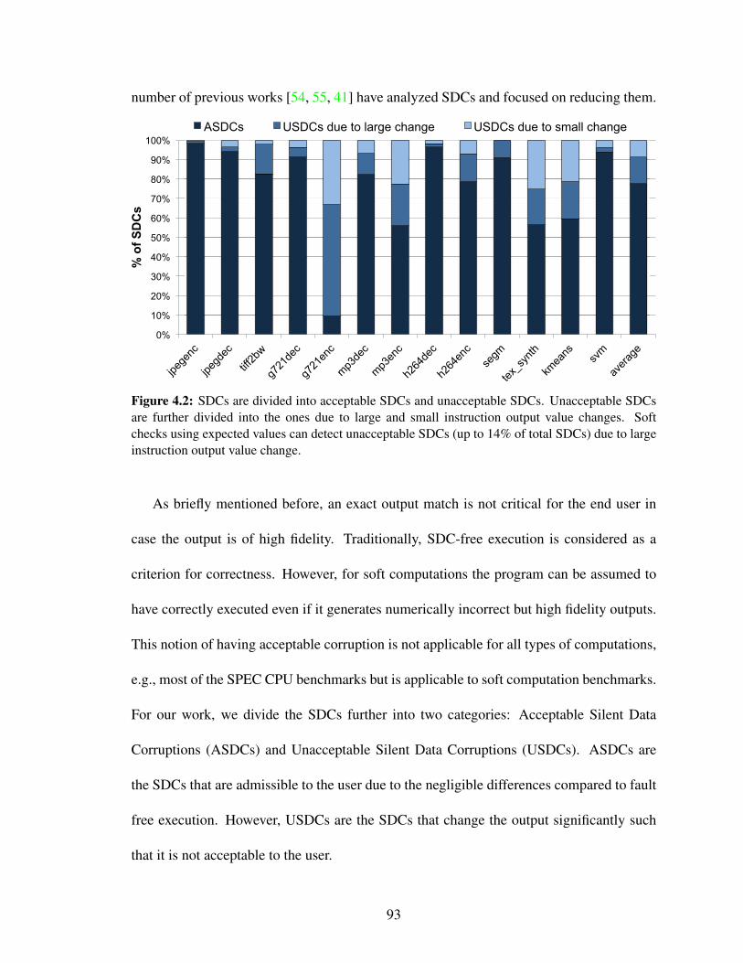
number of previous works [54, 55, 41] have analyzed SDCs and focused on reducing them.
0%
10%
20%
30%
40%
50%
60%
70%
80%
90%
100% %
of
SD
Cs
ASDCs USDCs due to large change USDCs due to small change
Figure 4.2: SDCs are divided into acceptable SDCs and unacceptable SDCs. Unacceptable SDCsare further divided into the ones due to large and small instruction output value changes. Softchecks using expected values can detect unacceptable SDCs (up to 14% of total SDCs) due to largeinstruction output value change.
As briefly mentioned before, an exact output match is not critical for the end user in
case the output is of high fidelity. Traditionally, SDC-free execution is considered as a
criterion for correctness. However, for soft computations the program can be assumed to
have correctly executed even if it generates numerically incorrect but high fidelity outputs.
This notion of having acceptable corruption is not applicable for all types of computations,
e.g., most of the SPEC CPU benchmarks but is applicable to soft computation benchmarks.
For our work, we divide the SDCs further into two categories: Acceptable Silent Data
Corruptions (ASDCs) and Unacceptable Silent Data Corruptions (USDCs). ASDCs are
the SDCs that are admissible to the user due to the negligible differences compared to fault
free execution. However, USDCs are the SDCs that change the output significantly such
that it is not acceptable to the user.
93
We performed fault injection experiments on unmodified soft computing benchmarks to
quantify the USDCs caused by faults that force large disturbance on the generated values by
instructions. The results of this experiment are presented in Figure 4.2. The experimental
setup and description of these benchmarks are presented later in Section 4.4. The Y-axis in
the graph plots total SDCs caused in the fault injection experiments. Each column is divided
into ASDCs and USDCs. USDCs are further divided into the SDCs that were due to a large
and small value changes in the corrupted instructions. On average, 77% of the SDCs result
in ASDCs and 14% in USDCs with large value changes. ASDCs are the errors that result in
user acceptable outputs and therefore nothing needs to be done for these. USDCs that are
caused by large output value change of a computation can be detected by having expected
value checks. Expected value checks, obtained by profiling (Section 4.3.3.1), make sure
that the output does not deviate outside a compact range. Although 14% might not seem
like a very large percentage but one must view this in the proper context as USDCs are the
worst of all.
4.3 Solution: Analysis and Design
4.3.1 Overview
We analyze a number of benchmarks to find out the most vulnerable computations in
soft applications to develop our compiler heuristics. These analyses involve fault injections
and then investigating fault propagation. The outcome of the program is correlated back to
the fault injection variable. Once these patterns are identified, we make compiler heuristics
to insert checking code in the application. As mentioned previously, all the computations in
94

a program are not soft computations. Precise computation of parts of the program that can
adversely affect the program output should be maintained. In our experiments we found
that the heuristics we have developed work well across a wide range of soft applications.
. . .f o r ( c r c = i n i t ; l e n >= 3 2 ; l e n −= 32){
r e g i s t e r u n s i g n e d long d a t a ;d a t a = m a d _ b i t _ r e a d (& b i t p t r , 3 2 ) ;
. . .t a b l e V a l = c r c _ t a b l e [ ( d a t a >> 24) ^ . . . ] ;c r c = ( c r c << 8) ^ t a b l e V a l ;
. . .}
. . .
Figure 4.3: The code snippet from mp3dec (mad) [50] benchmark. The variables that are dependenton their own values in the previous iterations are underlined. A corruption in such variables is morelikely to result in unacceptable outputs.
To show frequently occurring computations in soft computing applications, we show
a code snippet from mp3dec (mad) [50] benchmark in Figure 4.3. In our experiments
with various benchmarks, we have noticed that a corruption in the variables that carry
state across loop iterations is more likely to result in USDCs. We define such variables as
state variables and these variables are underlined in this figure. State variables include
loop iteration variables. Intuitively protecting state variables makes sense as state variables
have a snowball effect on the subsequent computations, because the error not only affects
the current iteration but it also propagates to future iterations. Protecting such variables
is critical to minimize the user unacceptable outputs because errors in these variables are
likely to cause significant changes in the output of a program. Loop index variables are also
state variables and an error in loop index variables have the potential to change the output
significantly by increasing or decreasing the number of iterations executed.
95
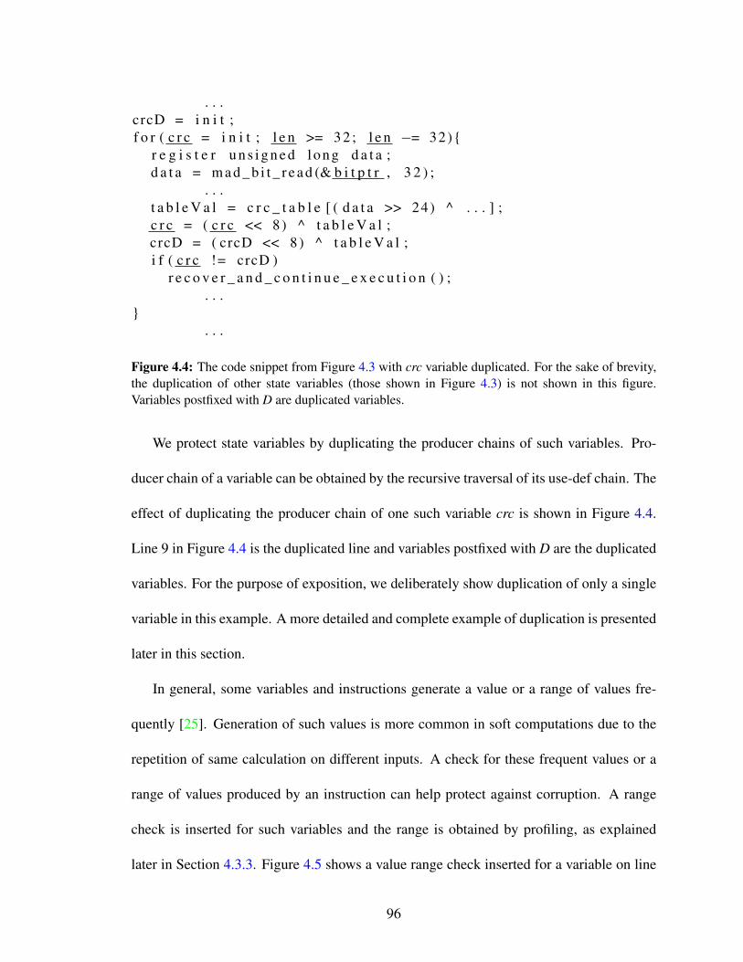
. . .crcD = i n i t ;f o r ( c r c = i n i t ; l e n >= 3 2 ; l e n −= 32){
r e g i s t e r u n s i g n e d long d a t a ;d a t a = m a d _ b i t _ r e a d (& b i t p t r , 3 2 ) ;
. . .t a b l e V a l = c r c _ t a b l e [ ( d a t a >> 24) ^ . . . ] ;c r c = ( c r c << 8) ^ t a b l e V a l ;crcD = ( crcD << 8) ^ t a b l e V a l ;i f ( c r c != crcD )
r e c o v e r _ a n d _ c o n t i n u e _ e x e c u t i o n ( ) ;. . .
}. . .
Figure 4.4: The code snippet from Figure 4.3 with crc variable duplicated. For the sake of brevity,the duplication of other state variables (those shown in Figure 4.3) is not shown in this figure.Variables postfixed with D are duplicated variables.
We protect state variables by duplicating the producer chains of such variables. Pro-
ducer chain of a variable can be obtained by the recursive traversal of its use-def chain. The
effect of duplicating the producer chain of one such variable crc is shown in Figure 4.4.
Line 9 in Figure 4.4 is the duplicated line and variables postfixed with D are the duplicated
variables. For the purpose of exposition, we deliberately show duplication of only a single
variable in this example. A more detailed and complete example of duplication is presented
later in this section.
In general, some variables and instructions generate a value or a range of values fre-
quently [25]. Generation of such values is more common in soft computations due to the
repetition of same calculation on different inputs. A check for these frequent values or a
range of values produced by an instruction can help protect against corruption. A range
check is inserted for such variables and the range is obtained by profiling, as explained
later in Section 4.3.3. Figure 4.5 shows a value range check inserted for a variable on line
96
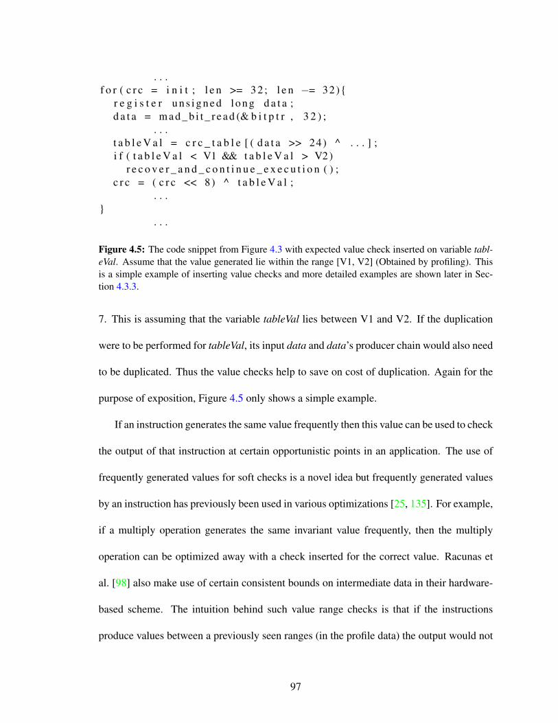
. . .f o r ( c r c = i n i t ; l e n >= 3 2 ; l e n −= 32){
r e g i s t e r u n s i g n e d long d a t a ;d a t a = m a d _ b i t _ r e a d (& b i t p t r , 3 2 ) ;
. . .t a b l e V a l = c r c _ t a b l e [ ( d a t a >> 24) ^ . . . ] ;i f ( t a b l e V a l < V1 && t a b l e V a l > V2 )
r e c o v e r _ a n d _ c o n t i n u e _ e x e c u t i o n ( ) ;c r c = ( c r c << 8) ^ t a b l e V a l ;
. . .}
. . .
Figure 4.5: The code snippet from Figure 4.3 with expected value check inserted on variable tabl-eVal. Assume that the value generated lie within the range [V1, V2] (Obtained by profiling). Thisis a simple example of inserting value checks and more detailed examples are shown later in Sec-tion 4.3.3.
7. This is assuming that the variable tableVal lies between V1 and V2. If the duplication
were to be performed for tableVal, its input data and data’s producer chain would also need
to be duplicated. Thus the value checks help to save on cost of duplication. Again for the
purpose of exposition, Figure 4.5 only shows a simple example.
If an instruction generates the same value frequently then this value can be used to check
the output of that instruction at certain opportunistic points in an application. The use of
frequently generated values for soft checks is a novel idea but frequently generated values
by an instruction has previously been used in various optimizations [25, 135]. For example,
if a multiply operation generates the same invariant value frequently, then the multiply
operation can be optimized away with a check inserted for the correct value. Racunas et
al. [98] also make use of certain consistent bounds on intermediate data in their hardware-
based scheme. The intuition behind such value range checks is that if the instructions
produce values between a previously seen ranges (in the profile data) the output would not
97

Figure 4.6: Instruction duplication in a single thread of execution. Instructions marked with doublecircle are duplicated instructions. The instruction marked with ld is a load instruction. We do notduplicate loads to save on memory traffic.
be significantly affected and is expected to be acceptable. These checks are soft checks in
the sense that they check the expected output values of instructions.
Overall, the foundation of our work is based on the following two observations:
1. First, if the program variables in the main loops of applications that have state across
iterations are corrupted, they are more likely to result in unacceptable output. Pro-
tecting these variables is critical for reducing USDCs.
2. Second, many soft computing benchmarks use the same calculations on different
inputs repeatedly such that generated values are in a range. If in presence of an
error, the value generated is within this range, it is probabilistically unlikely to have
a USDC in such a case. An expected value check on such instructions is inserted to
protect against soft errors.
98

Figure 4.7: Depending on the generated values, one of the three different types of value checks canbe inserted. Part (a) shows a single value check inserted if a single value is frequently generatedby an instruction. If two values are most frequently generated, the check in part (b) is inserted.However, if the values generated lie in a range, a range check as shown in part (c) is inserted.
4.3.2 Recomputing State Variables
State variables are a critical part of an application and corruption in these variables
propagates to subsequent iterations of the loop. They are protected by duplicating the pro-
ducer chain of such variables and then inserting a comparison between original producer
chain and duplicated producer chain of such variables. The technique to identify state vari-
ables is described in Section 4.4.1. Figure 4.6 shows an example of such a duplication
process in form of a data flow graph. Each circle represents an instruction (or destination
variable of that instruction). The solid arrows are data flow edges and dashed arrows repre-
sent inter-iteration loop dependences. The instructions marked with ld is a load instruction.
The instructions marked with double circle are duplicated instructions. The state variable
in this figure is variable 5. The producer chain of instruction 5 is duplicated as shown in
Figure 4.6(b). To save on memory traffic, the producer chain is terminated whenever a
load instruction is encountered. The reason for this is that a fault in data flow input for
load (address operand) is more likely to result in a symptom such as out-of-bound access.
Such symptoms can be used as an indication of soft error [41, 132] and a recovery can be
99
triggered.
4.3.3 Expected Value Checks
In soft computing benchmarks, same calculation on different inputs is performed re-
peatedly. Moreover, in general some instructions produce the same value almost all the
times [25]. To cover the values produced by an instruction, we devise three different types
of value checks as shown in Figure 4.7. Figure 4.7(a) shows the data flow graph before and
after the value checks are inserted. Instruction 1 produces the value V1 frequently so a check
with V1 is inserted. Similarly, Figure 4.7(b) shows the code before and after value checks
if the instruction generated two values V1 and V2 most frequently. Finally, Figure 4.7(c)
shows the data flow graph before and after a range check is inserted on an instruction that
produces values in a range [V1, V2]. To optimize the number of value checks, we came up
with two optimizations for long producer chains.
Optimization 1: A naive insertion of value checks on all the instructions that produce
values amenable for one of the checks in Figure 4.7 might lead to a prohibitively large
number of checks. Hence, to reduce the number of checks, we insert value checks deeper
in the producer chain. Figure 4.8 shows an example of such an optimization. If the values
produced by instruction 1, 3, 4 and 5 are amenable for value checks, a value check is only
inserted on the value produced by instruction 5.
Optimization 2: While duplicating instructions, if in a long producer chain, an instruc-
tion produces a value amenable to checks, the duplication is terminated and a value check
is inserted. An example of this is shown in Figure 4.9. In this example, instruction 4 pro-
duces value(s) or a range. In our duplication framework, if such a situation is encountered
100

Figure 4.8: Optimization 1 for long producer chains: this figure shows an example of a case wheremultiple instructions in the producer chain of an instruction are amenable for value checks. In orderto minimize on number of checks, value check should only be inserted for an instruction lower inthe producer chain.
the recursive duplication of producers is terminated and one of the value checks is inserted
instead.
Figure 4.9: Optimization 2 for long producer chains: if an instruction amenable to value check isencountered in producer chain, the duplication of producer chain of critical variables is terminatedat that point and a value check (vChk) is inserted as shown.
101

4.3.3.1 Value Profiling:
The frequent values or the range of values produced by an instruction are obtained us-
ing value profiling. In general, during the profile run, collecting all the values produced by
an instruction has very high overhead. An optimization to this is to maintain a fixed set of
most frequently produced values by each instruction. Since we also need a range of values
produced by an instruction, we have modified this traditional value profile. Essentially, we
require a histogram with bins as values produced corresponding to each instruction. How-
ever, the future values are unknown, so deciding the histogram bin size before running the
program is not possible. We have adopted a modified version of the On-line histogram algo-
rithm [14] for this purpose. Our adopted version of the algorithm is shown in Algorithm 2.
Input: A histogram h = ([lb1, rb1], m1), ... ([lbB, rbB], mB), a value vOutput: A histogram with B binsif v ∈ [lbi, rbi] for some i then
mi = mi + 1endelse
Add [v, v, 1] to the histogram h. Histogram h can now potentially have B+1bins;Sort the bins. Denote the sorted bins by ([lp1, rp2], m1), ... ([lpB+1, rpB+1],mB+1);Find a bin [lpi, rpi] that minimizes lpi+1 - rpi;Replace the bins ([lpi, rpi], mi), ([lpi+1, rpi+1], mi+1) by the bin([lpi, rpi+1], mi + mi+1);
endAlgorithm 2: Algorithm for obtaining histogram of the values produced by an instruc-tion.
The algorithm takes a histogram h of size B as an input. The number of bins B are pre-
decided and are set to 5 in our experiments. Initially the input histogram to this algorithm
can be empty. This histogram is maintained for every value generating instruction in the
102

program during profiling phase (a one time off-line process). ([lb1, rb1], m1) is a bin
frequency pair andm1 represents the number of values generated by a particular instruction
between and including lower bound of the bin (lb1) and upper bound of the bin (rb1).
Input: A histogram h = ([lb1, rb1], m1), ... ([lbB, rbB], mB) with sorted bins, athreshold on range Rthr
Output: A frequent range ([lp, rp], m)Pick a bin ([lbi, rbi], mi) such that mi = max(m1 ... mB);initialize retBin = ([lbret, rbret], mret) with ([lbi, rbi], mi);Denote the bin left to retBin by leftBin and the one to the right by rightBin;leftBin = ([lbleft, rbleft], mleft) and rightBin = ([lbright, rbright], mright);while (rbret - lbret < Rthr ) and still unconsidered bins do
if mleft ≥mright thenretBin = ([lbleft, rbret], mleft + mret);leftBin = next leftBin;
endelse
retBin = ([lbret, rbright], mret + mright);rightBin = next rightBin;
endendreturn retBin;
Algorithm 3: A greedy algorithm for obtaining compact range on the values producedby an instruction.
Once we have the bin-frequency pair for all the value generating instructions in an
application, the next step is to obtain a tight range of lower and upper bound where most
of the values generated by an instruction are concentrated. This information is calculated
and used while inserting the value checks in the application source code. This is obtained
by a greedy algorithm that works by picking a bin that has highest frequency and extends
this bin towards left or right while the range size lies within a threshold. This algorithm is
shown in Algorithm 3.
An important point to note here is that value profiling is an offline process (needs to
be done once per benchmark) and this overhead does not directly impact the performance
103

overhead of our technique. The frequent values or frequent range of values are obtained by
profiling the program on representative inputs. An application instrumented with expected
value checks might generate value check failures at runtime even if there are no errors
(false positives). However, this is not a correctness issue and could only lead to unwanted
recovery initiations. If a check fails, recovery from the check should be executed once and
if the same check fails again after recovery further recovery should not be executed for that
check. False positives rate is analyzed in Section 4.5.
4.4 Experimental Setup
We have evaluated our work by using Statistical Fault Injections (SFIs) into a microar-
chitectural model of a modern microprocessor. This same method is used by previous
works [41, 62, 90] to evaluate reliability solutions. SFI is performed by introducing bit
flips randomized in both time and space.
4.4.1 Source Code Transformations
We use the LLVM [66] compiler infrastructure to insert duplication code and expected
value checks into the application’s source code. At first, application source code is con-
verted into LLVM’s internal representation called LLVM IR (Intermediate Representation).
Our solution is implemented as a pass over LLVM IR. Passes operating at the IR level ei-
ther analyze the IR code or transform it from IR to IR, performing optimizations. Value
profiling is implemented as a separate pass. The IR is instrumented to collect value pro-
filing information. Our duplication pass uses information from other analysis passes such
104

Table 4.1: The benchmarks and their acceptable quality metrics.
Benchmark(BenchmarkSuite)
Description(Category)
Inputs Fidelity Mea-sure (Threshold)
train testjpegenc andjpegdec (media-bench [67])
A JPEG imageencoder and de-coder (image)
flower.ppmandflower.jpg
grid.ppmandgrid.jpg
Peak Signalto Noise Ratio(PSNR) (30 dB)
tiff2bw(mibench [50])
A tiff format toBW converter(image)
galaxy.tiff stars.tiff PSNR (30 dB)
segm (SD-VBS [128])
Image segmenta-tion (Computervision)
qcif sim_fast Segment matrixmismatch (10%)
tex_synth (SD-VBS [128])
Texture synthe-sis (Computervision)
qcif sim_fast Output matrixmismatch (10%)
g721enc andg721dec (media-bench [67])
audio encodingand decoding(audio)
universal.pcm clinton.pcm Segmental SNR(80 dB)
mp3encand mp3dec(mibench [50])
mp3 encodingand decoding(audio)
large.wav small.wav PSNR (30 dB)
h264enc andh264dec (media-bench II [43])
h264 video en-coding and de-coding (video)
foreman1.yuvand4CIF.264
foreman2.yuvandtest.264
PSNR (30 dB)
kmeans (in-house)
Clustering algo-rithm (Machinelearning)
color100 edge100 Cluster assign-ment mismatch(10%)
svm (svm-light [59])
Support vectormachine (Ma-chine learning)
train.dat test.dat Classification er-ror (10%)
105

as value profiling to produce bitcode with duplicated instructions and value checks. The
LLVM code generation framework is then used to generate ARM binaries from the modi-
fied bitcode. Identifying State Variables: LLVM IR is in Static Single Assignment (SSA)
form. At IR level, the state variables can simply be identified by looking the phi nodes
in loop headers. A phi node merges all the incoming versions of the variable to create a
new name for it. State variables have two incoming definitions—one from outside loop
definition and the other from inside loop updates—at loop headers and are represented by
phi nodes in loop headers.
4.4.2 Benchmarks and Fidelity Measures
We have collected a variety of benchmarks (a total of 13) that represent soft computa-
tions from various domains and at least two benchmarks from each of the following five
categories: image, audio and video processing; computer vision; machine learning. These
benchmarks represent a good mix of soft computations and we did not hand pick these
benchmarks to show a desirable behavior. A brief description of these benchmarks along
with their source benchmark suite is given in Table 4.1. Different inputs are used for pro-
filing and running the benchmarks. These profiling and test inputs are given in column 3 of
the table. Column 4 in the table shows the fidelity metric used to evaluate the quality of the
produced outputs. This is an application dependent metric and different metrics are used
for different benchmarks. Column 4 also shows the threshold used for acceptable quality
results. Higher PSNR represents a better quality image and video. We chose 30 dB as
threshold for PSNR and 80 dB for segmental SNR for acceptable quality. Similar thresh-
old values are used by Thomas et al. [126]. For machine learning and computer vision
106

benchmarks, outputs with more than 10% deviations are not considered acceptable. All
these benchmarks are compiled with their suggested compiler options. We use Clang [34]
as a frontend to generate bitcode for LLVM. Figure 4.10 shows the total number of state
variables, duplicated instructions and inserted value checks as a fraction of the total static
IR instructions. At most, only 11.4% of the static IR instructions are duplicated and only
8.3% of total static IR instructions have expected value checks on them.
!"#
$"#
%"#
&"#
'"#
(!"#
($"#
!"#$"%#%&'"(%&)*"+,"-.(%/0*)#.("
)*+*,#-+./# 012345+*,6# -+3#789/#
Figure 4.10: shows the total number of state variables, duplicated instructions and inserted valuechecks as a fraction of the total static IR instructions. The static code duplication and expected valuechecks are not more than 12% of the total static IR instructions.
4.4.3 Fault Model and Injection Experiments
The proposed approach is evaluated by injecting a number of faults in each application
run. The traditional single bit-flip [53, 73, 126, 41] in the processor state is used to model
transient faults. At a random cycle during the program execution, a register is randomly
selected first and then a randomly selected bit in that register is flipped. Wang et al. [133]
showed that, on aggregate, as much as 70% of the total failures due to faults in pipeline
107

structures such as register file, register alias tables, register free lists, instruction input and
output operands etc. results in register file inconsistencies. Thus, the register file is an
enticing target for fault injections and similar to previous works [41, 62], we evaluated
our work by injecting faults into the register file. Please note that protecting register file
by ECC would be able to cover faults occurring in register file itself but not the faults
that occur in other hardware structures and then propagate to register file. Overall, our
proposed technique is capable of handling faults in other microarchitectural units that affect
the program. A fault in a register can also affect the data dependent control flow. Our
solution have protection against such faults either by state variables duplication or by value
checks. However, it does not provide protection against faults that affect branch targets. For
protecting against branch target faults, a previously proposed [60] signature-based low-cost
solution can be used in conjunction with our proposed approach.
Table 4.2: GEM5 Simulator parameters (models an ARMv7-a profile of the ARM architecture).
Processor core @ 2GHzSimulation configuration out-of-order coreSimulation mode Syscall emulationPhysical integer register file size 256 entriesReorder Buffer Size 192 entriesIssue width 2
MemoryL1-D cache 64KB, 2-wayL1-I cache 32KB, 2-wayDTLB/ITLB 64 entries (each)
We used the GEM5 [16] simulator to simulate the workloads and implemented fault
injection infrastructure in this simulator. The simulator was run in ARM syscall emulation
mode and modeled the ARMv7-a profile of ARM architecture. The performance overheads
are obtained using an out-of-order model of the target processor and fault coverage results
108

are obtained using an atomic model of the target processor.
The details of the processor configuration for out-of-order model used for the experi-
ments are in Table 4.2. We injected a total of 13000 faults per technique to evaluate the
proposed solution, i.e. 1000 fault injection trials for each of the 13 benchmarks. Work by
Leveugle et al. [69] can be used to calculate the statistical significance of the fault injection
results. The calculation for our experimental setup shows that the with 95% confidence,
margin of error for fault coverage results is 3.1%. After the fault injection, the program
runs until completion. The result of each simulation trial is classified into one of the fol-
lowing five categories:
• Masked: The injected fault did not corrupt the program output. Application-level or
architecture-level masking occurred in this case. Also faults that generate acceptable
quality results are classified into this category.
• HWDetect: The injected fault produces a symptom such as a page fault so that
a recovery can be triggered. A fault is considered under this category only if the
symptom is produced within a number of cycles (1000 for our experiments) after the
fault was injected.
• SWDetect: The injected fault was detected by the software checks inserted at the
time of source code transformation.
• Failure: The injected fault resulted in out-of-bound address access and resulted in
program termination. Also, faults causing infinite loops in the program are classified
under this category.
109

0%
10%
20%
30%
40%
50%
60%
70%
80%
90%
100%
Orig
ina
l
Du
p o
nly
Du
p +
va
l ch
ks
Orig
ina
l
Du
p o
nly
Du
p +
va
l ch
ks
Orig
ina
l
Du
p o
nly
Du
p +
va
l ch
ks
Orig
ina
l
Du
p o
nly
Du
p +
va
l ch
ks
Orig
ina
l
Du
p o
nly
Du
p +
va
l ch
ks
Orig
ina
l
Du
p o
nly
Du
p +
va
l ch
ks
Orig
ina
l
Du
p o
nly
Du
p +
va
l ch
ks
Orig
ina
l
Du
p o
nly
Du
p +
va
l ch
ks
Orig
ina
l
Du
p o
nly
Du
p +
va
l ch
ks
Orig
ina
l
Du
p o
nly
Du
p +
va
l ch
ks
Orig
ina
l
Du
p o
nly
Du
p +
va
l ch
ks
Orig
ina
l
Du
p o
nly
Du
p +
va
l ch
ks
Orig
ina
l
Du
p o
nly
Du
p +
va
l ch
ks
Orig
ina
l
Du
p o
nly
Du
p +
va
l ch
ks
jpegdec jpegenc tiff2bw g721dec g721enc mp3dec mp3enc h264dec h264enc segm tex_synth kmeans svm average
% o
f to
tal fa
ult
s
Masked SWDetects HWDetects Failures USDCs
Figure 4.11: The fault outcome distribution among different categories is shown. Column originalshows the distribution for original unmodified code. The fault distribution with code duplication andcode duplication along with value checks is shown in Dup only and Dup + val chks, respectively.
• USDC: Faults that generate unacceptable data corruptions are classified into this
category. These are the SDCs that do not have acceptable output.
4.4.4 Recovery Support
The proposed solution is a soft error detection-only solution. Once a soft error is de-
tected, we rely on a recovery mechanism to recover from the detected error. Previously
proposed solutions such as Encore [42], a software-only recovery scheme can be used for
recovery. Checkpointing-based recovery schemes can also be used in conjunction with our
solution. Moreover, previous works [41, 132] propose that in future processors, recovering
from a checkpointed state of ∼1000 instructions would be required for aggressive perfor-
mance speculation. Such a recovery scheme, if available, can also be integrated with our
solution.
110

4.5 Experimental Evaluation and Analysis
Two of the most important parameters of any reliability scheme are its performance
overhead and provided fault coverage. We obtained performance overhead and fault cover-
age results using the experimental setup described in the above section. We use the simu-
lated runtime of the application as a performance measure and use this runtime to compare
the performance of different techniques. Our overall technique is a combination of critical
0%
10%
20%
30%
40%
50%
60%
% P
erfo
rm
an
ce
Ov
erh
ea
d
Dup only Dup + val chks
Figure 4.12: Performance overhead of checking by 1) duplicating the producer chain of state vari-ables. 2) duplicating the producer chain as well as inserting value checks wherever necessary.
variable checks by duplication and value checks. To analyze the contribution of each of
these, we present results for both.
Performance Overhead: Figure 4.12 shows the performance overhead measured in
terms of runtime. Dup only column shows the performance overhead if the duplication of
state variables is performed and no expected value checks are inserted. The mean perfor-
mance overhead of Dup only is only 7.6%. Dup + val chks column for each benchmark
111

shows the performance overhead if the duplication of the producer chains of state variables
and expected value checks are inserted. Dup + val chks also includes the two optimiza-
tions described in Section 4.3.3 that arise out of the interaction between duplication and
inserting value checks. The mean performance overhead for Dup + val chks is 19.6%.
Four benchmarks jpegdec, tiff2bw, mp3dec, h264dec and tex_synth see a relatively bigger
increase in performance overhead from Dup only because these benchmarks have a number
of instructions amenable for value checks. It is interesting to note that the overhead of svm
is lower for Dup + val chks than Dup only even though we found that the number of dy-
namic instructions are higher in Dup + val chks. This is due to the lower data cache misses
and branch mispredicts in the later case. The average overhead of full duplication tech-
nique (not shown in Figure 4.12) also used by Khudia et al. [62] is 57% for the benchmarks
used in our work. Full duplication is maximum amount of duplication possible without
duplicating loads/stores.
!"#
$"#
%!"#
%$"#
&!"#
&$"#
'!"#
'$"#
(!"#
($"#
)*+,+-./#
012#3-/4#
012#5#6./#789:#
)*+,+-./#
012#3-/4#
012#5#6./#789:#
)*+,+-./#
012#3-/4#
012#5#6./#789:#
)*+,+-./#
012#3-/4#
012#5#6./#789:#
)*+,+-./#
012#3-/4#
012#5#6./#789:#
)*+,+-./#
012#3-/4#
012#5#6./#789:#
)*+,+-./#
012#3-/4#
012#5#6./#789:#
)*+,+-./#
012#3-/4#
012#5#6./#789:#
)*+,+-./#
012#3-/4#
012#5#6./#789:#
)*+,+-./#
012#3-/4#
012#5#6./#789:#
)*+,+-./#
012#3-/4#
012#5#6./#789:#
)*+,+-./#
012#3-/4#
012#5#6./#789:#
)*+,+-./#
012#3-/4#
012#5#6./#789:#
)*+,+-./#
012#3-/4#
012#5#6./#789:#
;2<,=<7# ;2<,<-7# >?&@A# ,B&%=<7# ,B&%<-7# C2'=<7# C2'<-7# 8&D(=<7# 8&D(<-7# :<,C# E<FG:4-E8# 9C<.-:# :6C# .6<*.,<#
!"#$"$#$%&"'%(&$)"
H77<2E.@/<# IJ0K:#
Figure 4.13: Each column represents the silent data corruptions as a percentage of total faults. Thestacks in each column further divide the silent corruptions between acceptable program outputs andunacceptable data corruptions.
Fault Coverage: We analyze the fault coverage results for unmodified, Dup only and
Dup + val chks by injecting faults using the setup described in Section 4.4. If a fault results
112

in Masking, SWDetect or HWDetects, system can correctly execute the program. Hence,
fault coverage is defined as the percentage of injected faults that result in Masking, SWDe-
tect or HWDetects. First, faults are injected into original unmodified applications and their
outputs are classified among Masked, SWDetects, HWDetects, Failures and USDCs based
on the effect of the fault on the application execution. The results for this classification
are shown in Figure 4.11. Y-axis in the figure plots the percent of total injected faults into
an application. Results of fault injections into unmodified applications are shown in first
column (Original) for each benchmark. Original column does not have any SWDetects
because there are no software checks in the binary. Faults in unmodified applications gen-
erate 3.4% USDCs. Second, fault coverage of state variable only duplication is shown in
Dup only column. It improves fault coverage for all the benchmarks and reduces SDCs and
USDCs. Dup only, on average, has 1.8% USDCs. Finally, Dup + val chks column show
the fault coverage if the duplication of state variables along with expected value checks and
all optimizations are used. Dup + val chks has only 1.2% USDCs. We have also calculated
the USDCs for full duplication and this is not shown in a already dense Figure 4.11. The
USDCs rate for full duplication is 1.4% at 57% performance overhead. Please note that
loads/stores are not duplicated in full duplication, hence there are a number of faults that
escape detection. This result shows that selective duplication along with value checks is a
more efficient way than soft computation unaware full duplication to protect soft computa-
tion workloads.
Acceptable SDCs: Another important analysis is the number of acceptable outputs
among silent data corruptions. In this experiment, we break down the SDCs further be-
tween Acceptable SDCS (ASDCs) and Unacceptable SDCS (USDCs). Figure 4.13 shows
113
the result of this analysis for unmodified, Dup only and Dup + val chks. Each column in
Figure 4.13 represents the total number of SDCs for the corresponding benchmark. For ex-
ample, for kmeans 4.2% of the total injected faults into the unmodified (Original column)
application resulted in SDCs. Each column is further divided into ASDCS and USDCs.
On average, the SDCs are reduced from 15% down to 9.5% when going from Original
to Dup only while USDCs are reduced from 3.4% down to 1.8% for the same and SDCs
are reduced from 15% down to 7.3% when going from Original to Dup + val chks while
USDCs are reduced from 3.4% down to 1.2% for the same. It is interesting to note that
mp3enc and h264enc have higher SDCs for Dup + val chks than Dup only. This is due to
the interaction of code duplication for state variables and expected value checks. An opti-
mization (Optimization 2 in Section 4.3.3) that we implemented to minimize performance
overhead is to insert value checks instead of code duplication wherever beneficial in terms
of performance overhead. This, however, in some cases can result in more SDCs if critical
value checks are left out.
Sensitivity of results to different inputs: To ascertain the insensitivity of results to
input variations, we performed 2-fold cross-validation on our results. We switched test and
train inputs, i.e. test input was used to obtain profile data and train input was used in fault
injection runs, to obtain fault coverage results for Dup + val chks. We performed cross-
validation on jpegdec and kmeans from two separate fields. Cross-validation was performed
only on these two benchmarks due to a large number of runs required for obtaining fault
coverage results. The average performance overhead difference is 3%. The difference
between Masked, SWDetect, HWDetect, Failures and USDCs is only .2%, .45%, .05%,
.15% and .15%, respectively.
114

Impact of False Positives: A false positive occurs when one of the value checks fails
at runtime in the absence of a fault. In such cases, an unnecessary recovery needs to be
triggered. A high false positive rate increases the overhead due to unnecessary recoveries in
a fault detection and recovery system. For pipeline-flush based recovery, Racunas et al. [98]
calculate that 1 recovery initiation per 1000 instructions does not degrade the performance
significantly (2% to 6%). This degradation in performance is dependent on the particular
recovery technique. In comparison, in our case, the average false positive rate across all the
evaluated benchmarks is as low as 1 value check fail per 235K instructions. For our current
implementation, the profiling is done only on one input but the false positive rate can be
further reduced by combining profiling form multiple inputs and thus inserting checks only
on more stable invariant values.
Comparison with prior work: Thomas et al. [126] define the notion of Egregious Data
Errors (EDCs) for the outputs that deviate significantly from error-free outputs. Their work
develops heuristics for placing detectors by analyzing the pointer and control data affected
by a fault. In contrast, the main novelty of our scheme lies in the judicious combination
of selective use of expensive duplication for critical state variables and inexpensive value
checks for non-state parts of an application. The coverage of their scheme is measured
assuming ideal (100% detector accuracy (without implementing backward-slice duplica-
tion based error detectors). Memory dependence (reaching stores for loads) in backward
slice is not considered and hence coverage with actual implemented detectors is expected
to be lower. At 20% and 25% performance overhead (extra LLVM IR instructions) they
report a 85% and 86% coverage of EDCs with ideal detectors, respectively. In comparison,
even though it represents comparing IR instruction overhead and ideal detector coverage
115

with runtime overhead and actual detector coverage, our technique shows 82.5% actual
implemented detectors coverage of USDCs at 19.6% performance overhead (runtime).
4.6 Related Work
Li et al. [73] propose the notion of application level correctness and also introduce
the concept of acceptable quality. We have used acceptable output quality measure in
evaluating our work. The idea of user acceptable outputs has been used in previous re-
search [39, 10, 85] to trade-off between energy efficiency/execution time and output so-
lution quality. Li et al. [72] also previously proposed a light-weight recovery mechanism
and soft instruction classification. They show a fault coverage of 96% with relaxed defini-
tion of correctness in comparison to 97.8% of fault coverage of our solution. Performance
overhead of their technique is not reported in the paper. In comparison, we propose a tech-
nique to utilize the soft computing nature of applications and insert expected value checks
to propose a low cost fault detection solution.
There are a number of solutions proposed in the area of Software Implemented Hard-
ware Fault Tolerance (SIHFT). SWIFT [101] uses instruction duplication in a single thread
of execution. SWIFT protects the stores by duplicating their computation. Follow-up work
on SWIFT such as CRAFT and PROFIT [102] improved upon SWIFT by adding additional
hardware and Architectural Vulnerability Factor (AVF) analysis. However, the overhead of
SWIFT is 1.41x even on an aggressive ILP-friendly Intel Itanium processor( more favor-
able for exploiting ILP offered by interleaved duplication). Our proposed solution only has
19.6% performance overhead on a ARM processor.
116

Shoestring [41] used the idea of protecting only global stores in order to lower perfor-
mance overhead. Khudia et al. [62] improved Shoestring by utilizing profiling information.
Both of these solutions, unlike our solution, do not use the notion of user acceptable outputs
and do not incorporate application domain characteristics to increase the efficiency of their
proposed solution. We compare with error detector placement work by Thomas et al. [126]
in Section 4.5. Sundaram et al. [124] propose selective replication of instructions that has
30% to 75% performance overhead. Cong et al. [32] propose an approach to protect in-
structions based on their criticality. The technique is a combination of static analysis and
dynamic monitoring. The authors report energy savings and overhead of runtime monitor-
ing but a combined performance overhead for duplication and runtime monitoring is not
reported. Pattabiraman et al. [96] derived program level detectors using static analysis to
find the best location for detectors to be placed in program to avoid system crashes. They
identify certain properties such as fanout and lifetime from dynamic dependence graph of
the program for detector placement. Unlike our work, their focus is not on reducing the
large output corruptions but to avoid system crashes and in fault containment.
Likely program invariants have previously been used in checking validity of data streams,
detecting software bugs [37, 51, 136], to minimize the corruption of executing applica-
tions [97] and lower SDC rates due to permanent hardware faults [109]. Range-checks used
in this work are also a form of likely invariants. However, we combine range-based checks
with duplication to provide an effective transient fault detection solution. For transient
faults (usually a single-bit upset), range-based checks should be frequent while permanent
hardware faults continuously produce error hence sparing use of range-checks suffices.
Our solution is optimized to have low-overhead even though relatively frequent checks are
117

required to detect a single-bit upset. Other than high-cost high-reliability server class solu-
tions such as DMR (Dual-Modular Redundancy) and TMR (Triple-Modular Redundancy),
an approach to soft error reliability is Redundant Multithreading (RMT). Since processors
which can execute multiple threads simultaneously are increasingly commonplace, the idea
of using separate threads for error checking is a possibility. AR-SMT [108] introduced the
idea of RMT on SMT cores. The actual work is done by a leading thread, and the trailing
thread checks for the correctness. Subsequent works [100, 99] in this category have tried
to reduce the overhead of RMT still needing to run an extra thread for each existing thread
in the program. Shye et al. [121] explore process level redundancy in applications to pro-
vide transient fault detection. In comparison, our solution does not need to run any extra
thread/process to provide fault detection.
There exist a number of hardware based solutions to provide protection against soft
errors. In comparison, our solution is able to achieve high fault coverage with a low per-
formance overhead without needing any specific hardware additions. Racunas et al. [98]
present an hardware mechanism that can identify 85% of the injected faults to ensure that
much of the program intermediate data falls within certain bounds. Their use of bounds
on intermediate values in hardware is similar to our use of value checks in software. Ar-
gus [81] relies on a series of hardware checker units to perform online invariant checking
to ensure correct application execution. Lee et al. [68] propose hardware-based scheme
for partitioning failure critical and non-critical data into soft-error prone and soft-error
protected caches. Soft error detection by anomalous microarchitectural behavior has been
used by researchers to propose reliability solutions. Symptoms such as memory exceptions,
branch mispredicts and cache misses are used in ReStore [132] to detect soft errors. These
118

symptoms are an attractive way to detect soft errors at a relatively low cost. However,
fault coverage starts to saturate as more symptoms are included and performance overhead
starts rising. For example, using cache miss as a symptom might result in too many false
detections. mSWAT [53] presented a solution that detects anomalous software behavior to
provide a reliable system. mSWAT requires special simple hardware detectors to detect
faults. Our solution, however, uses only the available symptoms such as page faults to
classify faults under HWDetects category.
4.7 Conclusions
The relentless pursuit of technology scaling in order to gain performance, energy effi-
ciency and higher densities have made transistors more susceptible to soft errors. A grow-
ing number of applications from domains such as multimedia, computer vision, machine
learning etc. do not need their output to be 100% correct. This numerically incorrect but
acceptable output property of such applications can be exploited to provide an efficient
fault tolerant solution.
In this chapter, we propose a software-only solution that exploits the inherent fault tol-
erant nature of soft computing applications. Our solution duplicates producer chains of
certain critical variables and inserts expected value checks on other variables. We show
that a combination of these two is helpful in reducing the number of unacceptable silent
data corruptions. Overall, on average, SDCs are down from 15% to 7.3% and unaccept-
able SDCs are down from 3.4% to 1.2% in comparison to unmodified application. The
performance overhead of the proposed technique is only 19.6% and it does not require any
119

hardware modifications.
120

CHAPTER V
Rumba: An Online Quality Management System for
Approximate Computing
Soft applications mentioned in the previous chapter are inherently inaccuracy tolerant
to a certain degree. Hence, these are naturally amenable to approximate computing and
approximate computing can be employed to trade-off accuracy for energy efficiency/per-
formance gain for such applications. The approximated output of such applications, even
though not 100% numerically correct, is often either useful or the difference is unnotice-
able to the end user. However, a largely unaddressed challenge in the area of approximate
computing is quality control: how to ensure the user experience meets a prescribed level
of quality. Current approaches either do not monitor output quality or use sampling ap-
proaches to check a small subset of the output assuming that it is representative. While
these approaches have been shown to produce average errors that are acceptable, they often
miss large errors without any means to take corrective actions. In this chapter, we consider
application that are amenable to approximate accelerators and the output quality is defined
per-application basis.
121

5.1 Introduction
Computation accuracy can be traded off to achieve better performance and/or energy
efficiency. The techniques to achieve this trade off fall under the umbrella of approximate
computing. Algorithm specific approximation has been used in many different domains
such as machine learning, image processing, and video processing. Different algorithms
in these domains have been approximated by programmers to achieve better performance.
Video processing algorithms are good candidates for approximation as occasional varia-
tion in results will not be noticeable by the user. For example, a consumer can tolerate
occasional dropped frames or a small loss in resolution during video playback, especially
when this allows video playback to occur seamlessly. Machine learning and data analysis
applications also provide opportunities to exploit approximation to improve performance,
particularly when such programs are operating on massive data sets. In this situation, pro-
cessing the entire dataset may be infeasible, but by sampling the input data, programs in
these domains can produce representative results in a reasonable amount of time.
However, algorithm specific approximation increases the programming effort because
the programmer needs to write and reason about the approximate version in addition to the
exact version. Recently, to solve this issue, different software and hardware approximation
techniques have been proposed. Software techniques include loop perforation [2], approxi-
mate memoization [29, 110], tile approximation [110], discarding high overhead computa-
tions [111, 115], and relaxed synchronization [105]. Furthermore, there are many hardware
based approximation techniques that employ neural processing modules [40, 7], analog cir-
cuits [7], low power ALUs and storage [113], dual voltage processors [38], hardware-based
122

fuzzy memoization [5, 6] and approximate memory modules [114]. Approximation accel-
erators [40, 129, 36] utilize these techniques to trade off accuracy for better performance
and/or higher energy savings. In order to efficiently utilize these accelerators, a program-
mer needs to annotate code sections that are amenable to approximation. At runtime, the
CPU executes the exact code sections and the accelerator executes the approximate parts.
These techniques provide significant performance/energy gains but monitoring and
managing the output quality of these hardware accelerators is still a big challenge. A few of
the recently proposed quality management solutions include quality sampling techniques
that compute the output quality once in every N invocations [111, 10], techniques that build
an offline quality model based on the profiling data [10, 40].
However, these techniques have four critical limitations:
• As the output quality is dependent on the input values, different invocations of a
program may produce results of different output qualities. Therefore, sampling tech-
niques are not capable of capturing all changes of the output quality. Moreover, it
is highly possible to miss large output errors because only a subset of outputs are
actually examined, i.e., monitoring is not continuous. Also, profiling techniques do
not work efficiently if the profiling data is not representative of all possible inputs.
• Using these quality management techniques, if the output quality drops below an
acceptable threshold, there is no way to improve the quality other than re-executing
the whole program on the exact hardware. However, this recovery process has high
overhead and it offsets the gains of approximation.
• These techniques measure the quality of the whole output that is usually equal to the
123

average quality of each individual output element, e.g., pixels in an image. Previous
works [40, 7] in approximate computing show that most of the output elements have
small errors and there exist a few output elements that have considerably large errors,
even though the average error is low. These large errors can degrade the whole user
experience. For example, having a few pixels with high error in an image can be
easily noticed by a user. Existing quality management techniques treat all errors
equally but large errors have noticeable effect on the perceivable output quality.
• Tuning output quality based on a user’s preferences is another challenge for the
hardware-based approximation techniques. Different users and different programs
might have different output quality requirements. However, it is difficult to change
the output quality of an approximate hardware dynamically.
To address these issues, we propose a framework called Rumba∗, an online quality
management system for approximate computing [63]. Rumba’s goal is to dynamically
investigate an application’s output to detect elements that have large errors and fix these el-
ements with a low-overhead recovery technique. Rumba performs continuous light-weight
output monitoring to ensure more consistent output quality. Rumba’s design is based on
the following two observations:
First, approximation error can be accurately predicted by simple prediction models
such as linear, decision tree, and moving average. Second, we observe that code regions or
functions that are amenable for approximation are often pure. Pure code regions just read
their inputs and only write to their outputs without modifying any other state. Such sections
∗The name Rumba is inspired from Roomba R©, an autonomous robotic vacuum cleaner. It moves aroundthe floor and detects dirty spots on the floor to clean them.
124

can be safely re-executed without any side effects. It gives us the benefit of re-executing
the loop iterations to fix the erroneous output elements with low overhead.
Rumba has two main components: detection and recovery. The goal of the detection
module is to efficiently predict output elements that have large approximation errors. De-
tection is achieved by supplementing the approximate accelerator with a low-overhead error
prediction hardware. The detection module dynamically investigates predicted error to find
elements that needs to be corrected. It gathers this information and sends it to the recovery
module on the CPU. In order to improve the output quality, recovery module re-executes
the iterations that generate high error output elements.
To reduce Rumba’s overhead, recovery is done on the CPU in parallel to detection on
the approximate accelerator. The recovery module controls the tuning threshold to manage
output quality, energy efficiency and performance gain. The tuning threshold determines
the number of iterations that need to be re-executed.
The major contributions of this work are as follows:
• We explore three light-weight error prediction methods to predict the errors generated
by an approximate computing system.
• The ability to manage performance and accuracy trade offs for each application at
runtime using a dynamic tuning parameter.
• We leverage the idea of re-execution to fix elements with large errors.
• 2.1x reduction in output error with respect to an unchecked approximate accelerator
with the same performance gain. Detection and re-execution decrease the energy
savings of the unchecked approximate accelerator from 3.2x to 2.2x.
125

5.2 Challenges and Opportunities
The ability of applications to produce results of acceptable output quality in an approx-
imate computing environment is necessary to ensure a positive user experience. Output
quality control for approximate programs is important for the wide adaptation of this tech-
nology.
10%
80%
Error
Per
centa
ge
of
Outp
ut
Ele
men
ts
100%
100%
!"#$%&'##(#)
'*%+%,-.)
/+"**&'##(#)
'*%+%,-.)
Figure 5.1: Typical cumulative distribution function of errors generated by approximation tech-niques. A large number of output elements have small errors while a few output elements have largeerrors.
5.2.1 Challenges of Managing Output Quality
The following are the main challenges of output quality management in an approximate
computing environment.
126

(a) (b) (c)
Figure 5.2: An example of variation in image quality with the changing distribution of errors.Subfigure (a) is the original image without any errors. Ten percent of the pixels in (b) have 100%error while the rest of the pixels are intact. All pixels in (c) have 10% error. Although these twoimages have the same average quantitative output quality (90%), errors in Subfigure (b) are morenoticeable.
Challenge I: Fixing output elements with large errors is critical for user experience.
We analyze the distribution of errors in the output elements generated by an application
under approximation. Previous studies [40, 110, 111] reported that the Cumulative Distri-
bution Function (CDF) of the errors of an approximated application’s output follows the
curve shown in Figure 5.1. Figure 5.1 shows a typical CDF of errors in output elements
when total average error is less than 10%. This figure shows that the most of the output
elements (about 80%) have small errors (lower than 10%). However, there are few output
elements (about 20%) that have significant errors.
Although the number of elements with large errors is relatively small, they can have
huge impact on the user perception of output quality. Figure 5.2 demonstrates this. In this
figure, we generate two images by adding errors such that the overall average error is 10%
in both images. Figure 5.2(a) is the original image. In Figure 5.2(b), only 10% of pixels
have 100% errors while the rest of pixels are exact. On the other hand, all pixels in Fig-
ure 5.2(c) have about 10% error. Even though the overall output error is the same for both
127

the generated images, errors in Figure 5.2(b) are more noticeable than Figure 5.2(c) to the
end user. This shows that to effectively improve the output quality, a quality management
system should reduce the long tail of high errors.
Challenge II: Output quality is input-dependent. Another characteristic of approximate
techniques is that output quality is highly dependent on the input [40, 110, 111, 10]. In this
case, these techniques must consider the worst case to make sure that the output quality is
acceptable. To show this, we run an image processing application called mosaic that gen-
erates a large image using many small images. The first phase of this application computes
the average brightness of all input images. To approximate this phase, a well-known ap-
proximation technique called loop perforation [2] is used. Loop perforation drops iterations
of the loop randomly or uniformly. Therefore, in this case, instead of computing the aver-
age brightness of all the pixels, the approximate version computes the average brightness
of a subset of the pixels.
Figure 5.3 shows the output error for 800 different images of flowers [80]. Average
error of all the images is about 5% but there are many images that have output error above
the average, up to a maximum of 23%. Therefore, an approximate system in the worst case
(23% error) may produce unacceptable quality results. However, if a quality management
system can reduce the unacceptable outputs, the aggressiveness of approximate techniques
can be increased to get better performance and/or energy savings.
Also, since the output quality is highly input-dependent, previous quality managing
systems such as quality sampling or profiling techniques might miss invocations that have
low quality. In order to solve this problem, a dynamic light-weight quality management
system is required to check the output quality for all invocations.
128

0
5
10
15
20
25
0 100 200 300 400 500 600 700 800
Ou
tput
Err
or
Image
�������
�����
Figure 5.3: Mosaic application’s output error for 800 different images of flowers. This data showsthat the output quality is highly input-dependent.
Challenge III: Monitoring and recovering output quality is expensive. One of the chal-
lenges that all approximate techniques have is monitoring the output quality. In order to
solve this problem, continuous checks are necessary. Such checks cannot compute the exact
output, but instead need to be predictive in nature. Different frameworks [111, 10] suggest
running an application twice (exact and approximate versions) and comparing the results to
compute output quality. Unfortunately, it has high overhead and it is not feasible to monitor
all invocations. Running exact and approximate at all times will nullify the advantages of
using approximation.
To reduce this overhead, these frameworks utilize quality sampling techniques that
check the quality once in every N invocations of the program. Therefore, if the invoca-
tions that are not checked have low output quality, these frameworks will miss them due to
the input dependence of output quality (Challenge II).
129

Challenge IV: Different users and applications have different requirements on output
quality. In an approximation system, the user should be able to tune the output quality
based on her preferences or program’s characteristics. Software-based approximation tech-
niques are better at tuning the output quality. However, for hardware-based techniques, it
is a huge challenge. For example, in a system with two versions of functional units, exact
and approximate, it is hard to control the final output quality dynamically.
5.2.2 Rumba’s Design Principles
To overcome the four challenges, Rumba exploits two observations found in the kernels
that are amenable to approximation: predictiveness of errors and recovery by selective re-
execution.
0
0.2
0.4
0.6
0.8
1
-16 -11 -6 -1 4 9 14
Ou
tpu
t o
r A
pp
rox
ima
tio
n E
rro
r
(fra
ctio
n)
output approximate output errors
Figure 5.4: Exact output, approximate output and relative errors in the approximate output. Therelative errors in the approximate output are higher for some inputs than the others and are moreeasily predictable than the output itself.
Predictiveness of Errors: Rumba’s detection module is based on the observation that it is
possible to accurately predict the errors of an approximate accelerator using a computation-
130

ally inexpensive prediction model. Figure 5.4 shows exact output (a Gaussian distribution),
approximate output produced by an accelerator and errors in approximation. For this case,
it is visually clear that errors are concentrated on certain inputs. Hence, a simple prediction
model can separate cases of high errors accurately.
Rumba dynamically employs light-weight checkers to detect approximation errors. A
threshold on the predicted errors is used to classify errors in the output elements as high.
Therefore, Rumba targets output elements with high errors as mentioned in Challenge I.
Also, since Rumba has light-weight checkers, the checks can be performed online for all
the elements of each invocation (Challenge III).
Recovery by Selective Re-execution: In computing, a pure function or code region only
reads its inputs and only affects its outputs, i.e., it does not affect any other state. In other
words, pure functions or code regions can be freely re-executed without any side-effects.
Similar characteristics have been previously used in recovering program from external er-
rors simply by re-executing [42, 64]. Such functions or code regions naturally occur in
many data-parallel computing patterns such as map and stencil. We analyzed the data par-
allel parts of the applications in Rodinia benchmark suite [30] and found out that more than
70% of them can be re-executed without any side effects. Rumba detects this characteristic
using these previous techniques to identify such regions in applications. A more detailed
description of recovery is given in Section 5.3.1. It is not a new restriction imposed by
Rumba as previously proposed approximate accelerators [40, 7] require functions or code
regions to be pure to be able to map them to an approximate accelerator.
Therefore, if Rumba detects that one of the accelerator invocations generates output
elements with large error, the Rumba recovery module can simply re-execute that iteration
131

������
���
������ ��� ��
������ �����
����� ����
����� �
�������������
������
�� �������
����� �
��� �� �
�������� �������
������
��� � ������
������
������ �� ��
������
��� � ������
������
�������� �������
������
� ��� ��� � �
✶
�!!��"��� �
��� � �����
�����# � �����$ $ ✶ $ ✶ $ $
�%�� � � �
������ � �
����� ��� �
�� �
�! ����������
���!��� �� �
Figure 5.5: A high-level block diagram of the Rumba system. The offline components determinethe suitability of an application for the Rumba acceleration environment. The online componentsinclude detection and recovery modules. The approximation accelerator communicates a recoverybit corresponding to the ID of the elements to recompute with the CPU via a recovery queue.
to generate the exact output elements. In this case, there is no need to re-run the whole pro-
gram to recover those output elements (Challenge III). Also, using this technique, Rumba
can manage the performance/energy gains by changing the number of iterations to be re-
executed to target Challenge IV.
5.3 Design of Rumba
5.3.1 Overview
Approximation errors can be broadly divided into large errors and small errors. Ap-
proximation accelerators generate a large number of small errors and relatively few large
errors as shown in Figure 5.3. Rumba is a detection and recovery scheme for errors in an
approximate computing system. Rumba is specifically designed to detect these large errors
by a light-weight checker and then fix these errors. Rumba makes the output of an approx-
imation accelerator computing system acceptable by reducing the long tail of large errors.
Alternatively, with Rumba’s error correction capabilities, it will be possible to dial up the
amount of approximation, thus improving performance and/or energy savings, while still
132

producing user acceptable outputs.
A high-level block diagram of the Rumba system is shown in Figure 5.5. The offline
part of Rumba system consist of two trainers. The first trainer finds the optimal configura-
tion of the approximate accelerator for a particular source code. The second trainer trains
a simple error prediction technique based on the errors produced by the accelerator trainer.
The configuration parameters for both the approximate accelerator and the error predictor
are embedded in the binary.
The execution subsystem of Rumba is shown in the same figure. For the purpose of
exposition, we assume that the design of our approximation accelerator is similar to the
one proposed by Esmaeilzadeh et al. [40]. However, the same design principles can apply
to other accelerator based approximate computing systems. As shown in the figure, the core
communicates to the accelerator using I/O queues for data transfers from the core to the
accelerator and back from accelerator to the core. Rumba’s execution has two components:
detection and recovery modules.
The annotated approximate part of the application code gets mapped to the approxi-
mation accelerator [40, 7]. We augment the approximate accelerator by an error predictor
module to detect approximation errors. A variety of prediction techniques can be used
to predict these errors. We explore three light-weight checkers that are implemented us-
ing three simple error prediction techniques. These error predictors are described in Sec-
tion 5.3.2. Once a check fires, i.e., approximation for that particular output element is
larger than a tuning threshold (determined by the online tuner based on user requirements),
a recovery bit for the iteration generating that particular element is set in the recovery
queue as shown in Figure 5.5. The CPU collects these bits from the recovery queue and
133

re-executes the iterations that their recovery bit is set. Output merger choses the exact or
the approximate output as final result. A more detailed description is in Section 5.3.3. An-
other important aspect of Rumba is the dynamic management of output quality and energy
efficiency. By controlling the threshold at which the checker fires, Rumba can control the
number of iterations to be re-executed. This tuning process is discussed in Section 5.3.4.
5.3.2 Light-weight Error Prediction
An important first step is the inexpensive detection of large approximation errors in
output elements. Since it is not known beforehand which output elements will have large
errors, runtime checks should be employed for all the output elements. Therefore, the light-
weight nature of these checkers is of paramount importance. Complex checkers to detect
large approximation will offset the gains of approximation and, thus, are not desirable. A
desirable dynamic checker should have low overhead and still be accurate at predicting
errors in output elements.
A dynamic checker does not have access to the exact results, hence, the errors in ap-
proximate output cannot be computed by comparing with the exact result. Computing
exact values is not an option because that negates the benefits of employing an approxima-
tion system. The Rumba detection module needs to detect large approximation errors by
using inputs to the accelerator or the approximate output produced by the accelerator. We
call a method an input-based method if the method calculates errors using the inputs to the
accelerator. Similarly, if the errors are detected by just observing the accelerator output,
such a method is called an output-based method. For input-based methods, approximation
errors can be obtained using a simple predicting model on inputs in the following two ways:
134

• Errors by Value Prediction (EVP): predict the output using a model and then get the
error by comparing it with the approximate accelerator’s output.
• Errors by Error Prediction (EEP): predict the errors directly using a model.
In our experiments, we observed that if we use the same Prediction model it is more accu-
rate to predict the errors directly than computing the errors by first predicting the output.
We analyzed errors in the approximation of a Gaussian distribution and found that average
distance between exact approximation errors and errors obtained by EVP and EEP is 2.5
and 1, respectively, i.e., EEP is more accurate. Therefore, we use simple prediction mod-
els to predict errors in the approximation. We explore two input-based methods and one
output-based method to detect errors.
5.3.2.1 Error prediction using a linear model:
The first error prediction method is a linear error predictor and is an input-based method.
A linear error prediction method predicts error by computing a linear function of inputs to
the accelerator. Equation 5.1 shows the linear function that is calculated to compute the er-
ror. The number of terms (xis) are determined by the number of inputs to the code section
that is mapped to the approximate accelerator. A linear model requires relatively simple
computations in the form of multiply-add operations. Hence, the online prediction of errors
for a particular input does not add much energy overhead. The weights (wis) and constant
c are determined by offline training.
err = w0 ∗ x0 + w1 ∗ x1 ... wN−1 ∗ xN−1 + c (5.1)
135

where xi is the ith input, wi is the weight for the ith input and c is a constant.
5.3.2.2 Error prediction using a decision tree:
!"#$#%
"#
!&#$#%
&# !&#$#%
'#
())#*#+"#
!&#$#%
,#!&#$#%
-# !"#$#%
.#
())#*#+&#
())#*#+'#
())#*#+/#
())#*#+,#
())#*#+-#
())#*#+.#
())#*#+0#
!"#$#%
/#
Figure 5.6: A decision tree with a depth of 3 in decision nodes. For this example, it predicts errorsbased on two inputs. The leaf nodes (gray) give the approximation errors. The coefficients (cis andvis) are determined by offline training.
The second error prediction method is a decision tree and is also an example of input-
based methods. An example of error prediction using a decision tree is shown in Fig-
ure 5.6. This model contains decision and leaf nodes. The decision nodes typically have
two branches and uses one of the inputs to decide on whether to traverse the left or right
child. This process continues until it reaches a leaf node in the tree. Leaf nodes store the
predicted error. Training data is used to determine the values of constants used in making
decisions at the decision nodes and predicted error at the leaf nodes. The computation re-
quired in a decision tree is dependent on the depth of the tree structure. We limit the tree
depth to 7 in our experiments. Only comparison operations are required to implement this
decision tree and hence it is not a computationally expensive error prediction method.
136

5.3.2.3 Error prediction using moving average:
The third error prediction model is using moving average as the general trend of data
in the sequence. This moving average based method is an output-based method because
it just observes the accelerator outputs to find out the erroneous elements. The difference
between current element and the moving average can be used to detect large errors in a
number in the sequence. In this work, we used Exponential Moving Average (EMA) which
can be calculated by the formula shown in Equation 5.2.
EMA = (e ∗ α) + (Previous EMA ∗ (1− α)) (5.2)
where e = Current element, α = Smoothing factor = 21+N
and N = Number of elements in
the history
EMA computes the exponential moving average over a window of output elements and
compare it to each output element to compute the difference. If the difference is higher
than a tuning threshold, the detection module marks the output element as erroneous.
Once an application is deemed fit for approximation on the accelerator, it is transferred
to the accelerator augmented with an error predictor. The dynamic check for each output
element is the predicted error greater than a tuning threshold. If this predicted error is
greater than a tuning threshold, a large approximation error is suspected and the check
fires.
Predictor Hardware: Figures 5.7(a) and 5.7(b) show the hardware for the linear error
and decision tree error predictors. An approximate accelerator is augmented with these
hardware to predict errors. Coefficient buffers are circular buffers and contain weights and
137

����������������
����� ��
������
�����
������
����� �
����������
����������������
���
�����������
���������
������
����� ��
����
�������������� ��� �������!���
Figure 5.7: Hardware for the approximation error predictors.
constants for the linear model and decision constants and errors for the decision tree model.
The coefficients are transferred to these checkers via a config queue (the same queue is used
to transfer accelerator configuration) between the CPU and the accelerator.
EMA detects large approximation errors by comparing the current approximate outputs
with the history of previously computed approximate outputs. The history is represented
by EMA, the detection module keeps the EMA and calculates the approximate error in the
current approximate output by comparing it with EMA.
� � � � � � � �
� � � � � � � � � �
� � � �
��� �������
������ ���
���
�������� ������
Figure 5.8: An example of overlapping the re-computation of elements by the CPU with the ap-proximation accelerator. For example, a large error is detected in iteration 0 by the accelerator andthe CPU recomputes this iteration while accelerator is working on the execution of iteration 1 and2.
138

5.3.3 Low-overhead Recovery
Rumba’s recovery module on the CPU gets an iteration’s recovery bit via the recovery
queue. If the corresponding bit of an iteration is set, the recovery module re-executes
that iteration and commits the re-computed output while discarding the accelerator output
for that input. The results received by the CPU from the approximation accelerator are
directly committed to their final destination if the corresponding recovery bit is not set in
the recovery queue. This is how Rumba merges approximate outputs from the accelerator
with the exact outputs obtained by re-execution on the CPU.
The CPU and the accelerator work in a pipelined fashion, i.e., while accelerator is
working on an iteration, the CPU recomputes a previous iteration. An example of such an
arrangement is shown in Figure 5.8. For this example, the checks fire for output elements
of iterations 0, 2, 5 and 6. The CPU re-computes iteration 0 while the accelerator is work-
ing on iteration 1 and 2. Similarly, re-computation of iteration 2 is overlapped with the
execution of 3 and 4 on the accelerator and so on. In such a setup, the CPU can recompute
50% of the output elements, assuming a 2x gain for the accelerator, and still keep up with
the accelerator provided the elements to recompute are uniformly distributed.
5.3.4 Online Tuning
The tuning threshold of Rumba is used as a threshold for the dynamic checks to de-
termine if the current output has large error. A larger threshold value will result in fewer
iterations to be re-executed. This, in turn, will cause higher energy savings but lower out-
put quality. Rumba’s tuning threshold can be determined by user specified requirements
139

either on energy consumption or output quality. Online tuning can be programmed in three
modes:
TOQ Mode: In this mode, user specifies the target output quality (TOQ). The goal of
this mode is to make sure that all output elements have better quality than TOQ. Therefore,
Rumba compares the predicted quality with TOQ and re-execute iterations that have lower
quality than TOQ.
Energy Mode: If a user specifies an energy target to achieve, Rumba calculates the
number of iterations (iteration budget) it can re-execute while staying in the energy budget.
For each invocation, it monitors the number of re-executed iterations. If it goes over the
iteration budget it stops re-executing and increases the tuning threshold for the next invoca-
tion. If the current invocation is finished and Rumba still stays within the iteration budget,
the tuning threshold is decreased. This would result in more iterations to be re-executed
for the next invocation and thus improves output quality while staying in the same energy
budget.
Quality Mode: If a user is more concerned about achieving the best output quality,
Rumba maximizes re-execution of iterations on the CPU until the current invocation of
accelerator finishes. The accelerator performance gain in comparison to the CPU deter-
mines how many elements the CPU can recompute and still keep up with the accelerator.
If the CPU is not fully utilized during recovery, it implies that it can fix more iterations
so the tuning threshold is increased for the next invocation. If accelerator finishes the cur-
rent invocation and the CPU still has iterations to re-execute, the tuning threshold for the
next invocation is increased. This results in lesser number of re-executions for the next
invocation.
140

5.3.5 Error Detector Placement
!"#$%&'(")!"#$%&'(")
*+,$-").##"/"01($0)2)
3)
*+&'(4)
500$0)
60"78#($0)500$0)9)
(:0;))
<1=)
2)
3)
*+&'(4)
500$0)
60"78#($0)500$0)9)
(:0;))
<>=)
.##"/"01($0)?4"@'/)A'(&'()
Figure 5.9: Shows the design choices for the relative placement of input-based detectors withrespect to the accelerator. Configuration in part (a) adds delay, thus impacting overall performance,in the path to invoking accelerator. Configuration in part (b) wastes energy on invocations of theaccelerator that have large error.
An important design choice for input-based methods is the relative invocation of the er-
ror predictor with respect to the accelerator. An input-based detector can be placed in one
of the ways shown in Figure 5.9. Figure 5.9(a) (Configuration 1) shows the error detector
placement before sending the inputs to the accelerator and Figure 5.9(b) (Configuration 2)
shows the error detector placement if the error detector and accelerator simultaneously start
working on inputs. These configurations provide different trade-offs in the design space.
Configuration 1 saves the unnecessary accelerator invocations, hence saves energy, for the
cases when error detector detects an error. However, since error prediction precedes the ac-
celerator invocation, it delays accelerator computation, hence, has performance overhead.
Energy is wasted in Configuration 2 for accelerator invocations that have errors greater than
the threshold. However, error detector in this configuration does not add any delay in the
invocation of the accelerator, hence, does not add to performance overhead. In our exper-
iments, to minimize the impact on performance overhead, we use Configuration 2. Error
detector placement for output-based methods is straight forward and should be invoked
after accelerator invocation.
141
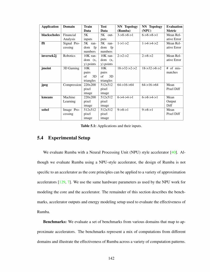
Application Domain TrainData
TestData
NN Topology(Rumba)
NN Topology(NPU)
EvaluationMetric
blackscholes FinancialAnalysis
5Kinputs
5K out-puts
3->8->8->1 6->8->8->1 Mean Rel-ative Error
fft Signal Pro-cessing
5K ran-dom fpnumbers
5K ran-dom fpnumbers
1->1->2 1->4->4->2 Mean Rel-ative Error
inversek2j Robotics 10K ran-dom (x,y) points
10K ran-dom (x,y) points
2->2->2 2->8->2 Mean Rel-ative Error
jmeint 3D Gaming 10Kpairsof 3Dtriangles
10Kpairsof 3Dtriangles
18->32->2->2 18->32->8->2 # of mis-matches
jpeg Compression 220x200pixelimage
512x512pixelimage
64->16->64 64->16->64 MeanPixel Diff
kmeans MachineLearning
220x200pixelimage
512x512pixelimage
6->4->4->1 6->8->4->1 MeanOutputDiff
sobel Image Pro-cessing
512x512pixelimage
512x512pixelimage
9->8->1 9->8->1 MeanPixel Diff
Table 5.1: Applications and their inputs.
5.4 Experimental Setup
We evaluate Rumba with a Neural Processing Unit (NPU) style accelerator [40]. Al-
though we evaluate Rumba using a NPU-style accelerator, the design of Rumba is not
specific to an accelerator as the core principles can be applied to a variety of approximation
accelerators [129, 7]. We use the same hardware parameters as used by the NPU work for
modeling the core and the accelerator. The remainder of this section describes the bench-
marks, accelerator outputs and energy modeling setup used to evaluate the effectiveness of
Rumba.
Benchmarks: We evaluate a set of benchmarks from various domains that map to ap-
proximate accelerators. The benchmarks represent a mix of computations from different
domains and illustrate the effectiveness of Rumba across a variety of computation patterns.
142

We use the same set of benchmarks as used in the NN accelerators [40, 7]. A brief descrip-
tion of these benchmarks along with their domain, train and test data is given in Table 5.1.
Rumba NN (Neural Network) topology column in the table shows the NN topology used by
Rumba. For example, 6->4->4->1 for kmeans implies that the NN has 6 inputs, two hidden
layers of 4 neurons each and 1 output. The final column in this table shows the NN topology
used by the unchecked NPU. In all cases, Rumba’s error detection capabilities make it pos-
sible to chose a smaller or equal, therefore efficient, NN. The output quality of applications
is usually measured by an application specific error metric [111, 110, 40]. This application
specific error metric is given in the evaluation metric column in Table 5.1. We use Mean
Pixel Difference for images and target a 90% output quality because SAGE showed that
more than 86% of the images (from an image quality assessment database [118, 138]) with
quality loss (according to Mean Pixel Difference metric) less than 10% were equivalent to
“Good” or “Excellent” ratings by human subjects. 90% output quality is in commensurate
with the previous works in approximate computing [40, 10, 113].
Accelerator Output: We obtain the accelerator output (approximate output) by imple-
menting NN using pyBrain [116] library. We find the best NN configuration by searching
the NN topology space. The best configuration for our case is the smallest NN that does
not produces excessive errors. The NN topology space is large thus the NN we consider
have at most 2 layers and the number of neurons are restricted to at most 32 neurons in
each layer (same restriction as in NPU [40]).
Energy Modeling: We run each application using the GEM5 [16] simulator to calculate
the different microarchitectural activities. These activities are fed to McPAT [119], which
calculates the baseline energy for the entire application. We use an X86-64 model for the
143

Parameter Value Parameter ValueFetch/Issue width 4/6 Load/Store Queue Entries 48/48INT ALUs/FPUs 2/2 L1 iCache 32KBLoad/Store FUs 1/1 L1 dCache 32KBIssue Queue Entries 32 L1/L2 Hit Latency 3/12 cyclesROB Entries 96 L1/L2 Associativity 8INT/FP Physical Registers 256/256 ITLB/DTLB Entries 128/256BTB Entries 2048 L2 Size 2 MBRAS Entries 16 Branch Predictor Tournament
Table 5.2: Microarchitecutral parameters of an X86-64 cpu used in experiments.
cpu core and the microarchitectural parameters are given in Table 5.2. The accelerator
design is an 8-Processing Elements (PEs) NPU and uses the same parameters for various
structures of the PEs as given in the NPU paper [40]. We model the energy of the multiply-
and-add for the linear error model and comparator in the same way as in the NPU paper. We
calculate the energy for the light-weight checkers separately. The energy of these checkers
and the energy of re-computation of elements on the CPU are combined to calculate the
total energy for a particular scheme.
5.5 Evaluation
We evaluate Rumba for output quality, energy savings, false positives and the coverage
of large errors. We also analyze the energy savings of Rumba for different target output
qualities.
5.5.1 Output Quality
Output Error: Output errors are measured using the application specific metric given
in Table 5.1 on the whole application output. Figure 5.10 shows the output error with
respect to the number of output elements fixed for different techniques under consideration.
144

!"
#!"
$!"
%!"
!" &!" #!!"
!"
'"
("
#$"
#)"
!" &!" #!!"
(a) blackscholes (b) fft (c) inversek2j (e) jmeint
(f) jpeg (g) kmeans (h) sobel
Percentage of fixed elements
Ou
tpu
t E
rro
r
!"
#!"
$!"
%!"
'!"
!" &!" #!!"
!"
#!"
$!"
%!"
!" &!" #!!"
!"
'"
("
#$"
#)"
!" &!" #!!"
!"
&"
#!"
#&"
$!"
!" &!" #!!"
!"
#!"
$!"
%!"
!" &!" #!!"
*+,-." /-0+12" 3045162" 789" .40,-676616:" ;6,,76616:"
Figure 5.10: Output error with respect to the number of output elements fixed.
Output error is directly related to the output quality. Output error of 5% represents 95%
output quality. The y-axis of each plot in this figure shows the output error, while the x-axis
shows the number of elements that need to be fixed to achieve that particular output error.
Random fixes a given percentage of randomly selected output elements. For example, for
fixing 10% of the elements Random selects 10% of output elements randomly and then
recomputes them. Similarly, Uniform shows the output error when a given percentage of
output elements to be fixed are chosen uniformly among all output elements. Ideal has the
oracle knowledge about the approximation errors in all the output elements and it uses this
oracle knowledge to fix a given percentage of the output elements. The data for Ideal is
generated by sorting approximation errors in output elements by the error magnitude and
then fixing the highest error elements. For example, to obtain output error when 10% of
the elements are fixed for the Ideal scheme, the top 10% approximation error elements are
fixed. Finally, EMA, linearErrors and treeErrors represent the output error when the errors
145
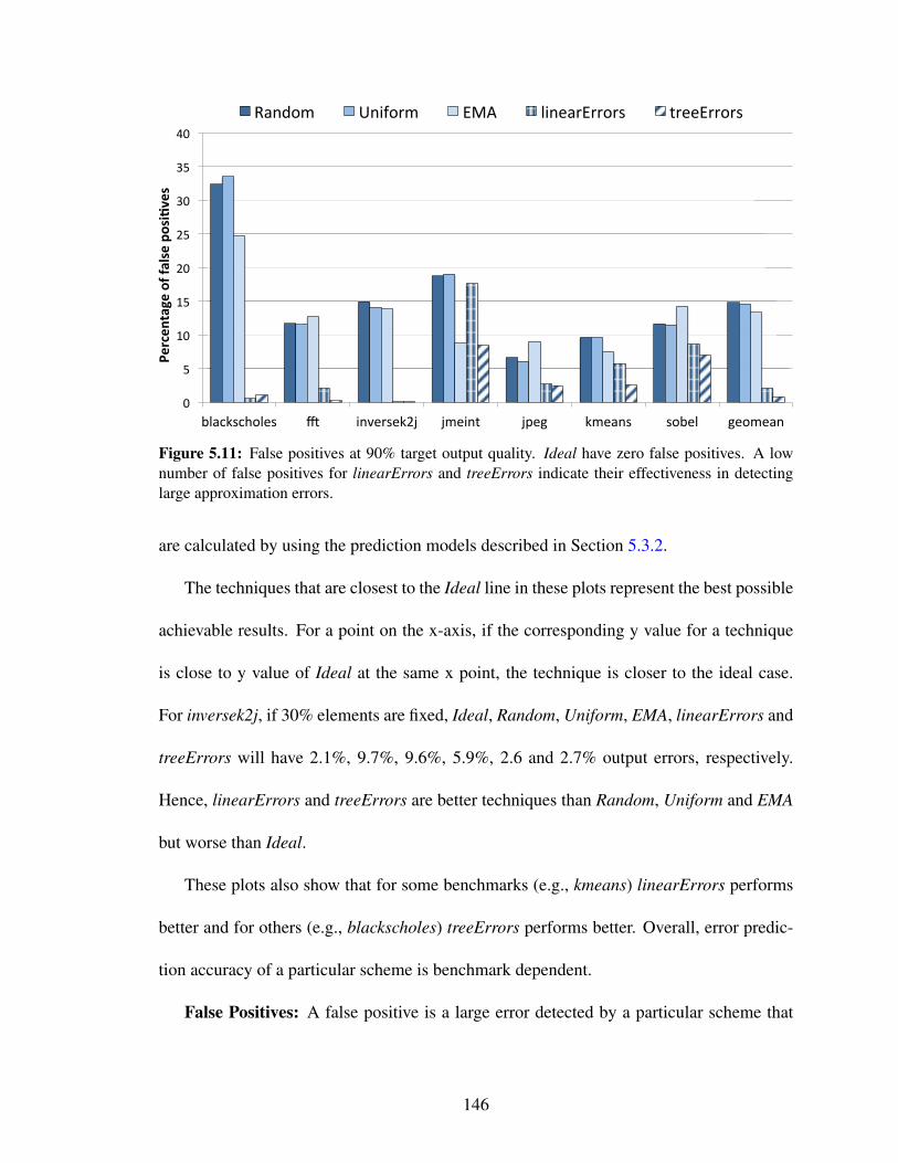
!"
#"
$!"
$#"
%!"
%#"
&!"
&#"
'!"
()*+,-+./)0-" 1" 23405-0,%6" 670238" 690:" ,70*3-" -/(0)" :0/70*3"
!"#$"%&'(")*+)+',-").*-/01"-)
;*3</7" =32>/57" ?@A" )230*5?55/5-" 8500?55/5-"
Figure 5.11: False positives at 90% target output quality. Ideal have zero false positives. A lownumber of false positives for linearErrors and treeErrors indicate their effectiveness in detectinglarge approximation errors.
are calculated by using the prediction models described in Section 5.3.2.
The techniques that are closest to the Ideal line in these plots represent the best possible
achievable results. For a point on the x-axis, if the corresponding y value for a technique
is close to y value of Ideal at the same x point, the technique is closer to the ideal case.
For inversek2j, if 30% elements are fixed, Ideal, Random, Uniform, EMA, linearErrors and
treeErrors will have 2.1%, 9.7%, 9.6%, 5.9%, 2.6 and 2.7% output errors, respectively.
Hence, linearErrors and treeErrors are better techniques than Random, Uniform and EMA
but worse than Ideal.
These plots also show that for some benchmarks (e.g., kmeans) linearErrors performs
better and for others (e.g., blackscholes) treeErrors performs better. Overall, error predic-
tion accuracy of a particular scheme is benchmark dependent.
False Positives: A false positive is a large error detected by a particular scheme that
146

was not actually a large error. An error prediction scheme will have a false positive if
the predicted error is high but the actual error is not. It is important to have low numbers
of false positives for a technique for it to be practical. A high number would imply that
the CPU would need to fix a large number of elements thus partially offsetting the gains
of approximation. Figure 5.11 shows the number of false positives for 90% target output
quality, i.e., 10% output error in output elements. For example, the first bar from the left
for the blackscholes benchmark represents 32% false positives for Random if we target
90% output quality. Random and Uniform have a large percentage of false positives since
these techniques randomly and uniformly, respectively, pick approximate output elements
to fix and do not have any detection method. Ideal does not have any false positives since
it has oracle knowledge of the errors in output elements. On average, Ideal, Random,
Uniform, EMA, linearErrors and treeErrors have 0%, 14.8%, 14.5%, 13.3%, 2.1% and
.76% false positives for 90% target output quality. linearErrors and treeErrors show a very
low percentage of false positives and thus are effective at detecting large approximation
errors.
Fixed Elements: Figure 5.12 shows the number of elements that are need to be fixed
(recomputed) to achieve 90% output quality. A lower number of fixes implies that the
energy overhead of re-execution on the CPU will be lower. Hence, a technique that fixes
lower number of elements to achieve the same quality is better. For example, on average,
Random requires 41% (29% more than Ideal) of the output elements to be fixed to achieve
10% output error. In comparison to Ideal, linearErrors and treeErrors just require 9% and
6% extra elements to be fixed to achieve the same output quality, respectively.
Large Error Coverage: Relative coverage is defined as the normalized ratio of de-
147
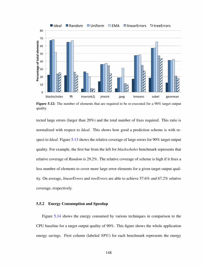
!"
#!"
$!"
%!"
&!"
'!"
(!"
)!"
*!"
+,-./0.12,30" 4" 5673803/$9" 9:356;" 9<3=" /:3-60" 02+3," =32:3-6"
!"#$"%&'(")*+)&*&',)","-"%&.)
>?3-," @-6?2:" A65B28:" CDE" ,563-8C88280" ;833C88280"
Figure 5.12: The number of elements that are required to be re-executed for a 90% target outputquality.
tected large errors (larger than 20%) and the total number of fixes required. This ratio is
normalized with respect to Ideal. This shows how good a prediction scheme is with re-
spect to Ideal. Figure 5.13 shows the relative coverage of large errors for 90% target output
quality. For example, the first bar from the left for blackscholes benchmark represents that
relative coverage of Random is 29.2%. The relative coverage of scheme is high if it fixes a
less number of elements to cover more large error elements for a given target output qual-
ity. On average, linearErrors and treeErrors are able to achieve 57.6% and 67.2% relative
coverage, respectively.
5.5.2 Energy Consumption and Speedup
Figure 5.14 shows the energy consumed by various techniques in comparison to the
CPU baseline for a target output quality of 90%. This figure shows the whole application
energy savings. First column (labeled NPU) for each benchmark represents the energy
148

!"
#!"
$!"
%!"
&!"
'!!"
()*+,-+./)0-" 1" 23405-0,#6" 670238" 690:" ,70*3-" -/(0)" :0/70*3"
;0)*<40"+/405*:0"/=")*5:0"055/5-"
;*3>/7" ?32=/57" @AB" )230*5@55/5-" 8500@55/5-"
Figure 5.13: Relative coverage of large errors at 90% target output quality. Ideal has 100% cover-age.
savings of the unchecked NPU, i.e., no error checking mechanism is employed. NPU [40]
reduces, on average, the CPU energy consumption by 3.2x. Note that since NPU does
not have any fixing mechanism for large errors and so the output application quality is not
always 90%. Without fixing any errors, output error, on average, is 20.6%. The other bars
from left to right for each benchmark show energy consumed by Ideal, Random, Uniform,
EMA, linearErrors and treeErrors schemes, respectively. The energy consumption shown
for each of the schemes in this figure includes energy required to recompute the elements on
the CPU and also the energy required for the checkers in the accelerator. As also observed
in the NPU work [40], kmeans has very little energy gains and achieves slowdown because
the code region that gets mapped to the NPU is very small and can be efficiently executed
on the CPU itself. Energy savings of sobel decrease significantly for linearErrors and
treeErrors schemes because this particular benchmark requires relatively large number of
re-executions due to the lower prediction accuracy of errors.
149

!"
#"
$"
%"
&"
'"
()*+,-+./)0-" 1" 23405-0,$6" 670238" 690:" ,70*3-" -/(0)" :0/70*3"
!""#$%&'()*+),-./*0,12%'()*
;<=" >?0*)" @*3?/7" =32A/57" BCD" )230*5B55/5-" 8500B55/5-"
$&E%"
#$E&"
##EF"
#$E%"
Figure 5.14: Energy consumption of Rumba, including the cost of re-computation and the en-ergy used for the prediction of large approximation errors. treeErrors saves 2.2x energy while theunchecked NPU saves 3.2x energy.
Figure 5.15 shows the speedup all the schemes described earlier. Each scheme also
factors in performance loss due to re-execution on the CPU if the CPU cannot keep up
with the accelerator. Since Rumba (linearErrors or treeErrors) overlaps recovery on CPU
with the accelerator execution, it is able to maintain the same speedup (2.1x) as the NPU.
Our energy savings and speedup for the NPU baseline are close to the ones given in the
NPU paper [40] but do not exactly match as we use different neural network libraries and
simulation infrastructure.
Time for prediction: Figure 5.16 shows the time taken by the two error predictor
model normalized with respect to the NPU. For all the benchmarks, linearErrors and
treeErrors require less time than the NPU. Therefore, the predicted error is always avail-
able before NPU finishes and the NPU never needs to wait for the error predictor to finish,
i.e., error prediction does not slow down the NPU.
150

!"
#"
$"
%"
&"
'"
("
)*+,-.,/0*1." 2" 34516.1-$7" 781349" 7:1;" -81+4." .0)1*" ;1081+4"
!""#$%&'()*+",,-."*
<=>" ?@1+*" A+4@08" >43B068" CDE" *341+6C6606." 9611C6606."
Figure 5.15: Speedup of each technique with respect to the CPU baseline. Rumba (linearErrors ortreeErrors) maintains the same speedup (2.2x) as the NPU.
Rumba reduces approximation errors overall by 2.1x (20.6% to 10%). Rumba achieves
this error reduction while maintaining the same performance improvement as the NPU ac-
celerator but reduces the energy savings from 3.2x to 2.2x in comparison to the unchecked
NPU.
5.5.3 Case Studies
Energy vs. Output Quality: Figure 5.17 shows the energy consumption of different
schemes with varying requirements on output quality for the fft benchmark. Energy savings
for the unchecked NPU for fft is 3.3x. As expected, Ideal achieves the best energy savings
among all techniques. treeErrors achieves energy savings close to the Ideal scheme for
higher target error rates (> 7%). Note that the gap between treeErrors and Ideal increases
as the demands on output quality increases ( greater than 97%). This is because Ideal
knows exactly which elements to fix to achieve certain target output quality while treeEr-
151

!"
!#$"
!#%"
!#&"
!#'"
("
)*+,-.,/0*1." 2" 34516.1-$7" 781349" 7:1;" -81+4." .0)1*" ;1081+4"
!"#$%&'()*+#,-.$)+
<=>" *341+6?6606." 9611?6606."
Figure 5.16: Time used by error prediction models in comparison to the NPU. This is normalizedwith respect to the NPU. Error prediction model are faster in all the cases, hence, the acceleratornever needs to wait for the error prediction model to finish execution.
rors (or linearErrors) must predict such cases. This causes the false positives for treeErrors
(or linearErrors) to start increasing, requiring more re-computation and more energy con-
sumption. Thus, the gap between Ideal and treeErrors (or linearErrors) is larger at high
demands on output quality.
CPU Activity: In this second case study, we show an example of the CPU activity
in conjunction with the accelerator. The top half of Figure 5.18 shows the percentage
difference of each output element (on y-axis) with treeErrors for 200 elements (on x-axis).
To achieve 10% target output error, a tuning threshold of 0.33 is required on this percentage
difference (y-axis). The bottom half of the figure shows the CPU activity. The accelerator
and the CPU work in tandem, i.e., the CPU fixes the detected large approximation errors
while the accelerator executes other iterations. Only 30 elements out of these 200 (15%)
are above this threshold and thus the CPU can keep up with an approximate accelerator as
fast as 6.67x.
152

���
���
���
���
���
� � � � ��
������������ ������������������
���������� �
���
�
�����
�������������
���
Figure 5.17: Energy consumption vs target error rate for fft.
5.6 Related Work
Approximate computing, where the accuracy is traded off for better performance or
higher energy efficiency, is a well-known technique. Approximate computing techniques
can be broadly classified into two categories: Software-based and hardware-based ap-
proaches. Software-based approaches are usually algorithmic modifications and can be
utilized without any hardware modifications. Loop perforation [2] is one of the well-
known software approximation techniques which skips the iterations of loops randomly
or uniformly. Rinard et al. [107] use early phase termination technique to terminate paral-
lel phase as soon as there are too few remaining tasks to keep the processor busy to prevent
the processors from being idle and wasting energy. Sartori et al. [115] introduce a software
approximation technique which targets control divergence on GPUs. Paraprox [110] is a
software framework which detects patterns in data parallel applications and applies dif-
ferent approximation techniques such as loop perforation, approximate memoization, and
153

0
0.5
1
Per
centa
ge
Dif
fere
nce
0.33
�������
������
0
1
0 50 100 150 200
CP
U A
ctiv
ity
Output Elements
Figure 5.18: The approximation accelerator and the CPU work in tandem. The CPU works onre-computing detected large error iterations while the accelerator continues with the execution. Inthis case, 0.33 is the tuning threshold used to achieve 10% target error rate.
tile approximation based on the detected patterns. All these software approximation tech-
niques need a quality management system to monitor the output quality and control the
aggressiveness of the approximation during execution.
Different hardware approximation techniques have also been proposed to save energy
while improving performance. EnerJ [113] proposed hardware techniques such as volt-
age scaling, width reduction in floating point operations, reducing DRAM refresh rate, and
reducing SRAM supply voltage to reduce energy consumption. Esmaeilzadeh et al. [38]
demonstrated dual-voltage operation, with a high voltage for precise operations and a low
voltage for approximate operations. The low-voltage pipeline introduces faults in the oper-
ations and hence these operation are approximate. We compare against the hardware neural
network [40] proposed by the same authors extensively in our results section. Du et al. [36]
also use hardware neural networks to trade off accuracy for energy savings. Amant et al. [7]
154

design limited precision analog hardware to accelerate approximable code sections. Other
works [125, 129] design different approximate accelerators. Sampson et al. [114] improve
memory array lifetime using approximation. Flikker [74] is an application-level technique
that reduces the refresh rate of DRAM memories which store non-critical data. The Rumba
quality management system can be added to these hardware-based approximation tech-
niques to control and improve their output quality.
There exist a few quality management solutions to control quality in an approximate
computing system. Ansel et al. [8] use a genetic algorithm to find the best approximate
code that provides the acceptable quality. In this work, the programmer writes runtime
low overhead checking functions to verify output quality online. However, Rumba can
automatically manage the output quality without programmer’s help. CCG [112] is another
quality monitoring technique. In this technique, while GPU runs the approximate version,
the CPU is responsible to check the quality of a subset of data for the next invocation. To
reduce the performance overhead of monitoring, size of the subset that is processed by the
CPU is small and thus, CCG’s accuracy to predict the output quality is limited. Unlike
CCG, Rumba has light-weight checkers and therefore, it can investigate larger subset of
the data compared to CCG.
Green [10] is a framework that developers can use to take advantages of approximation
opportunities to achieve better performance or reduce energy consumption. Green builds a
quality of service model based on the profiling data that gets used at runtime. In order to
make sure that output quality is acceptable, Green checks the output quality once in every
N invocations. SAGE [111] is an approximation framework for GPUs that automatically
generates approximate versions of the input program using skipping atomic expressions,
155

compressing data, and tile approximation. SAGE also uses a similar quality sampling
strategy as Green to check the output quality frequently. However, in contrast to these
techniques, because of its light-weight checkers, Rumba checks all invocations to reduce
large errors and to make sure that the output quality is acceptable for all invocations. Some
other techniques [26, 27, 106, 104, 83] statically analyze applications assuming an input
distribution to reason about the output quality under approximation. Such techniques do
not need sampling but can only handle limited computational patterns and approximation
methods.
PowerDial [56] is a framework that dynamically monitors the application’s perfor-
mance during runtime. When the performance drops below target performance, PowerDial
will increase the aggressiveness of the approximation to match the performance require-
ments. Their goal is to maximize accuracy while maintaining application’s performance.
Several probabilistic reasoning models [84, 27, 22, 103, 29] are also introduced to compute
the probability of the output being wrong. In contrast, Rumba dynamically monitors the
output quality during runtime and recovers from the large errors generated by an approxi-
mation technique.
Hardware reliability for soft computations and approximate computing share the same
basic underlying philosophy. Hardware reliability solutions [61, 126, 72] for soft computa-
tions aim to allow errors in error tolerant parts of an application with the goal of lowering
the cost of reliability. The idea of re-execution has previously been used in the context of
reliability to recover against hardware faults [33, 42]. We leverage this idea in the con-
text of recovering against approximation errors and it fits well with the nature of the code
regions (pure) that are mapped to approximate accelerators.
156

5.7 Conclusions
Approximate computing can be employed for an emerging class of applications from
various domains such as multimedia, machine learning and computer vision. Approximate
computing trades off accuracy for better performance and/or energy efficiency. However,
the quality control of approximated outputs has largely gone unaddressed. In this chapter,
we propose Rumba for online detection and correction of large errors in an approximate
computing environment.
Rumba predicts large approximation errors by light-weight checkers and corrects them
by recomputing individual elements. Our results demonstrate that Rumba is effective at
predicting large errors and follows an ideal case very closely. Across a variety of bench-
marks from different domains, we show that Rumba reduces the output error by 2.1x in
comparison to an accelerator for approximate programs while maintaining the same per-
formance improvement. To achieve this, the Rumba framework reduces the energy savings,
on average, from 3.2x to 2.2x in comparison to an unchecked accelerator.
157

CHAPTER VI
Neural Accelerator and Checker Design Space Exploration
Previous chapter shows that error prediction is feasible, cheap and practical to build. It
also demonstrated the predictability of approximation errors with the help of cost effective
and simple methods. Most of the errors in approximate accelerators are small but large
errors do matter for approximate computing. Approximation errors can be effectively pre-
dicted using input-based simple prediction methods (e.g., decision tree) or output-based
methods (e.g., EMA). We deliberately restricted the error prediction models to be decision
tree and linear methods in the previous chapter to keep the cost of checkers low. How-
ever, another neural network can also be used to predict errors of the neural accelerator.
However, that raises several interesting questions. For example, how big the size of such
a neural network checker can be before we nullify the gains of approximation? This chap-
ter explores the answer to this question and related trade-offs of accelerator and a neural
network checker.
158

6.1 Introduction
Error prediction is an effective method to control the large errors produced by an ap-
proximate accelerator, e.g. a Neural Processing Unit (NPU). Error prediction can also be
performed using another neural network. Let us first take a look the process of training a
neural checker in the context of approximation error prediction. Figure 6.1 shows how we
train an error prediction method. First, using a set of inputs, the NPU model is trained.
Once an NPU model is obtained, approximate outputs are produced using a second set of
train input. Errors are calculated by comparing the exact output for second training set and
approximate output. Now this second set of inputs and calculated errors are used to train
another neural network to obtain the error predictor model. This model is used to predict
errors online on a previously unseen test set.
Using another neural network is particularly interesting if the NPU is constructed from
a neural fabric. If we have a computation fabric that can be configured to construct neural
network of different sizes, the NPU and the checker can be constructed from the same fab-
ric. In such a case, a natural question is what is the trade off between the size of the NPU
and the size of checker? In this chapter, the design space of the accelerator and checker
is investigated. This chapter of the dissertation investigates the answers to following ques-
tions:
• Does some application become amenable to approximation if we use an error checker?
• Is it better to have a big NPU and no error checker or an NPU combined with an error
checker?
159

!"#$%&$#'()*+$
)*,-#./%-#,-#.$0'()*$123$
123$4%5"6$
!"#$%&$#'()*7$
)*,-#.$
8(69-6(#"$
:''%'.$
0'()*$:''%'$
2'"5)9#%'.$
:''%'$2'"5)9#%'$
;%5"6.$
<-#,-#$=(,,'%>?$
:>(9#$4%5"6$<-#,-#$=">(9#?$
Figure 6.1: Shows the steps to train an error predictor.
• Can a combination of an NPU and an error checker provide better quality and better
energy efficiency?
• Given a neuron computation fabric, how can we divide the neurons among the NPU
and the checker to get better output quality along with energy efficiency, i.e., should
more neuron be allocated to the NPU or more to the checker?
6.2 Exploration Setup
As briefly mentioned, the idea is to explore the co-design of accelerator and the error
checker design. We also aim to analyze various trade offs related to error and energy ef-
ficiency of such a co-design. To answer the questions raised in Section 6.1, we trained
different configuration of neural checkers and decision trees of various depths. These con-
figuration were then evaluated in conjunction with various NPU configuration for output
error and energy cost analysis. The neural network topology space is large thus the NN
we consider have at most 2 layers and the number of neurons are restricted to at most 128
neurons in each layer. For each layer the number of neurons considered are 1, 2, 4, 8, 16,
160

32, 64 or 128 for the NPU configuration as well as checker configuration. Thus, we have
72 (8 (one layer only) + 8*8 (two layers)) total configurations for the NPU and similarly
72 configuration of the checker for each NPU configurations. Hence, total configurations
explored are 5184 (72*72) for NPU vs NN checker. For example, let us assume if NPU
configuration has two hidden layers of size 32 each. For this configuration, each of the 72
NN configuration were trained as error predictor and the cost versus error trade offs are
analyzed. Decision tree checkers were restricted to a max depth of 7 to restrict the number
of total designs.
6.3 Experimental Results
Figure 6.2 shows energy cost versus error for different NPU versus NN and decision
tree checker configurations for Blackscholes benchmark. Each circle on this graph is a
combination of a particular configuration for the NPU and a particular configuration of the
NN checker. For example, a point on this graph can corresponds to an NPU configuration of
two hidden layers of 32 neurons each and a checker NN configuration that have 8 neurons
in a single layer. The points represented by indexed square are the configurations that does
not have any checker, i.e., these are NPU only design points. A single square on this graph
shows the error and cost for no accelerator, i.e., all the computations are performed exactly
on the CPU. Points shown by a cross sign correspond to an NPU and decision tree of certain
depth. On the x-axis of this graph is the cost of a configuration relative to the CPU. CPU
has a cost of 1 and output error of 0% as shown in the figure. In this figure, output error for a
configuration is shown on the y-axis. The number in the box corresponding to each design
161
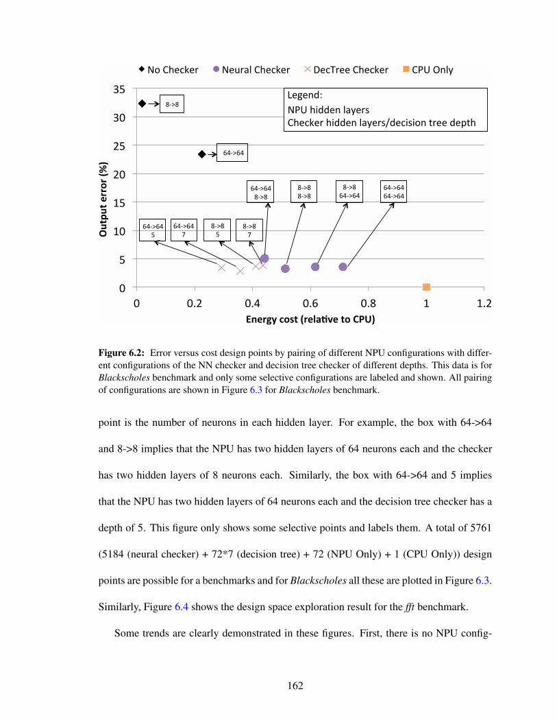
!"
#"
$!"
$#"
%!"
%#"
&!"
&#"
!" !'%" !'(" !')" !'*" $" $'%"
!"#$"#%&''('%)*
+%
,-&'./%0(1#%)'&2345&%#(%678+%
+,"-./01/2" +/3245"-./01/2" 6/072//"-./01/2" -89":;5<"
)(=>)("
*=>*"
*=>*"
*=>*")(=>)("
*=>*"
*=>*"
)(=>)(")(=>)("
)(=>)("
+89".?@@/;"54</2A"
-./01/2".?@@/;"54</2AB@/0?A?,;"C2//"@/DC."
E/F/;@G"
)(=>)("
H")(=>)("
#"
*=>*"
#"*=>*"
H"
Figure 6.2: Error versus cost design points by pairing of different NPU configurations with differ-ent configurations of the NN checker and decision tree checker of different depths. This data is forBlackscholes benchmark and only some selective configurations are labeled and shown. All pairingof configurations are shown in Figure 6.3 for Blackscholes benchmark.
point is the number of neurons in each hidden layer. For example, the box with 64->64
and 8->8 implies that the NPU has two hidden layers of 64 neurons each and the checker
has two hidden layers of 8 neurons each. Similarly, the box with 64->64 and 5 implies
that the NPU has two hidden layers of 64 neurons each and the decision tree checker has a
depth of 5. This figure only shows some selective points and labels them. A total of 5761
(5184 (neural checker) + 72*7 (decision tree) + 72 (NPU Only) + 1 (CPU Only)) design
points are possible for a benchmarks and for Blackscholes all these are plotted in Figure 6.3.
Similarly, Figure 6.4 shows the design space exploration result for the fft benchmark.
Some trends are clearly demonstrated in these figures. First, there is no NPU config-
162
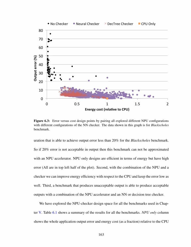
!"
#!"
$!"
%!"
&!"
'!"
(!"
)!"
*!"
!" !+'" #" #+'" $"
!"#$"#%&''('%)*
+%
,-&'./%0(1#%)'&2345&%#(%678+%
,-"./01203" ,04356"./01203" 7018300"./01203" .9:";<6="
Figure 6.3: Error versus cost design points by pairing all explored different NPU configurationswith different configurations of the NN checker. The data shown in this graph is for Blackscholesbenchmark.
uration that is able to achieve output error less than 20% for the Blackscholes benchmark.
So if 20% error is not acceptable in output then this benchmark can not be approximated
with an NPU accelerator. NPU only designs are efficient in terms of energy but have high
error (All are in top left half of the plot). Second, with the combination of the NPU and a
checker we can improve energy efficiency with respect to the CPU and keep the error low as
well. Third, a benchmark that produces unacceptable output is able to produce acceptable
outputs with a combination of the NPU accelerator and an NN or decision tree checker.
We have explored the NPU-checker design space for all the benchmarks used in Chap-
ter V. Table 6.1 shows a summary of the results for all the benchmarks. NPU only column
shows the whole application output error and energy cost (as a fraction) relative to the CPU
163

!"
#"
$!"
$#"
%!"
%#"
&!"
&#"
!" !'%" !'(" !')" !'*" $" $'%" $'(" $')"
!"#$"#%&''('%)*
+%
,-&'./%0(1#%)'&2345&%#(%678+%
+,"-./01/2" +/3245"-./01/2" 6/072//"-./01/2" -89":;5<"
Figure 6.4: Error versus energy cost design points for the fft benchmark.
for an efficient NPU configuration that has no checker. Half error design column shows the
error and energy cost for a Pareto-optimal npu-checker design that has approximately half
the error of NPU only design. The last column in this table also shows the checker type that
is able to achieve the given half error design. Table shows N/A for Half error design for the
sobel benchmark. sobel has very low error with almost all the configuration of the NPU,
hence, we do not get much benefits of using of a checker with this benchmark. The results
in this table demonstrate that the best checker type to achieve 50% less error is application
dependent.
Overall, the results show that NPU-checker co-design provides many choices and a user
can pick a design based on the error requirements for a particular application.
164

NPU only Half error designApplication Output error Energy cost Output error Energy cost Checker Type
(%) (x) (%) (x)blackscholes 21.53 .07 10.78 0.42 Decision Treefft 12.69 .05 6.42 0.12 Decision Treeinversek2j 12.92 .01 6.49 0.09 Decision Treejmeint 35.89 .04 17.27 0.49 Neural Networkjpeg 19.49 .02 10.02 0.47 Neural Networkkmeans 10.41 .28 5.98 0.82 Neural Networksobel 0.46 .03 N/A N/A N/A
Table 6.1: Summary of design space exploration results. NPU only column shows the applicationoutput error and cost relative to the CPU for an efficient NPU configuration that has no checker.Half error design column shows the error and cost for a Pareto-optimal NPU-checker design thathas approximately half the error of the NPU only design.
6.4 Conclusions
In this chapter, the design space of the NPU accelerator and the checker is explored.
The design space exploration highlights few important trade offs. For some benchmarks,
an NPU-only design might not give acceptable output error. In such cases, a combination
of the NPU and checker is a good alternative. We can obtain different design points that
have different error versus energy efficiency trade-offs. Overall, NPU combined with a
checker is a better accelerator design than the NPU accelerator alone.
165

CHAPTER VII
Conclusions and Future Directions
As transistors are becoming smaller and smaller, integrated circuits constructed out of
these transistors are becoming increasingly susceptible to transient faults. Traditional so-
lutions to protect against these failures are expensive in terms of performance/energy/area
overheads. In this thesis, I have proposed low-cost software only methods to protect against
transient faults for applications from various domains. These methods intelligently com-
bine traditional duplication and other novel ways of symptom generation to detect transient
faults (Chapter II, III and IV).
Also, in the path of performance scaling, energy has become the limiting factor [21].
Therefore, designers have started to explore alternative methods such as heterogeneous
cores and accelerator for achieving energy efficiency and improving performance. At the
same time, a class of emerging applications from domains such as multimedia, machine
learning, computer vision do not require 100% numerically correct output. Many of these
applications either compute on sensor data and/or produce results that have subjective in-
terpretations, i.e., the quality of the output is subjectively judged by a human. These two
trends of marginal gains in energy efficiency by scaling and increasing number of approx-
166

imate applications go well with each other. Approximate computing is at the intersection
of both of these trends and works by trading off accuracy of application outputs to achieve
energy efficiency and/or improve performance. A slew of approximation solutions has
recently been proposed [40, 111, 115, 2]. A key challenge for such systems is to provide
acceptable quality of outputs. Providing acceptable output quality is critical in making such
systems practical. We propose Rumba for online detection and correction of large errors in
an approximate computing environment (Chapter V). The co-design of the accelerator and
the error checker is explored in Chapter VI.
One of the main themes of this thesis is the exploitation of anomalies to provide accept-
able results. Anomalies can be used to construct systems with good enough answers using
inexact components. Such systems with good enough answers are going to be a norm in
the future as these are efficient and faster. Many of the methods and ideas explored in this
thesis can be further expanded and combined with other ideas in a variety of contexts. In
Chapter IV, the method to find out the variables that are going to cause unacceptable silent
data corruptions is based on heuristics. Bornholt et al. [22] proposed an interesting of repre-
senting uncertainty and finding out the distribution of program variables. This uncertainty
information can be combined with the heuristics developed in Chapter IV to improve the
coverage of unacceptable silent data corruptions.
We have explored quality control using error prediction methods in the context of an
accelerator based approximate computing environment. We believe that error prediction
is an equally feasible technique for other approximation methods such as Truffle architec-
ture [38] that has two pipelines: a high voltage pipeline for exact operations and a low
voltage pipeline for inexact operations. For example, a prediction method can be trained
167

to predict if an operation is going to make large error on the low voltage pipeline. If this
happens to be the case, such an operation can be executed on the high voltage pipeline.
The large errors are fixed using prediction methods in the hope that they improve the
perceived and average output quality. However, a still challenging problem in this area is
to find out how exactly intermediate results affect the final output quality of an application.
Finding a solution to this problem is a practically useful direction of further research.
An attractive area of research that was explored in Chapter VI is the accelerator design
space. It shows the usefulness of error prediction. The chapter demonstrates that some of
the applications that produce unacceptable quality with the accelerator alone, and hence
hitherto deemed as not amenable to approximation, can take advantage of approximation
with the help of error prediction methods. An interesting direction is to find out which
applications become amenable to approximation with a combined design of an accelerator
and error prediction methods.
We have explored hardware checkers for quality control in approximate computing
because they are energy efficient. Software checkers can also be used, however, an open
question is the effect of software checkers on total energy savings. Along the similar lines,
the whole NPU can be implemented in software as well. Esmaeilzadeh et al. [40] reported
that the overhead of a software implementation of the NPU, on average, is 20x for the
evaluated benchmarks. However, we postulate that a special and highly optimized software
implementation can outperform if the amount of computation approximated by the neural
network is significant. No such benchmarks exist in the current set of evaluated benchmarks
but finding out a set of such benchmarks is a worthy direction of research.
Let us assume that the code region approximated on the accelerator is a loop and has N
168

inputs and M outputs. We can unroll the loop the k times and can construct an NPU with kN
inputs and kM outputs instead of just N inputs and M outputs. A fascinating question and
a direction of research is finding out the scenarios where such loop unrolling is beneficial
in terms of the quality of output results.
169

BIBLIOGRAPHY
170

BIBLIOGRAPHY
[1] M. Abadi, M. Budiu, U. Erlingsson, and J. Ligatti. Control-flow integrity principles,
implementations, and applications. ACM Trans. Inf. Syst. Secur., 13(1):4:1–4:40,
Nov. 2009. 84
[2] A. Agarwal, M. Rinard, S. Sidiroglou, S. Misailovic, and H. Hoffmann. Using code
perforation to improve performance, reduce energy consumption, and respond to
failures. Technical Report MIT-CSAIL-TR-2009-042, MIT, Mar. 2009. 122, 128,
153, 167
[3] A. Aho, M. Lam, R. Sethi, and J. Ullman. Compilers: principles, techniques, and
tools, volume 1009. Pearson/Addison Wesley, 2007. 59
[4] Z. Alkhalifa, V. Nair, N. Krishnamurthy, and J. Abraham. Design and evaluation of
system-level checks for on-line control flow error detection. TDPS, jun 1999. 55,
80, 81
[5] C. Alvarez, J. Corbal, and M. Valero. Fuzzy memoization for floating-point multi-
media applications. IEEE Transactions on Computers, 54(7):922–927, 2005. 123
[6] C. Alvarez, J. Corbal, and M. Valero. Dynamic tolerance region computing for
multimedia. IEEE Transactions on Computers, 61(5):650–665, 2012. 123
171

[7] R. S. Amant, A. Yazdanbakhsh, J. Park, B. Thwaites, H. Esmaeilzadeh, A. Hassibi,
L. Ceze, and D. Burger. General-purpose code acceleration with limited-precision
analog computation. In Proc. of the 41st Annual International Symposium on Com-
puter Architecture, page To Appear, 2014. 2, 122, 124, 131, 133, 142, 143, 154
[8] J. Ansel, Y. L. Wong, C. Chan, M. Olszewski, A. Edelman, and S. Amarasinghe.
Language and compiler support for auto-tuning variable-accuracy algorithms. In
Proc. of the 2011 International Symposium on Code Generation and Optimization,
pages 85 –96, 2011. 155
[9] T. Austin. Diva: a reliable substrate for deep submicron microarchitecture design.
In Proc. of the 32nd Annual International Symposium on Microarchitecture, pages
196–207, 1999. 13
[10] W. Baek and T. M. Chilimbi. Green: a framework for supporting energy-conscious
programming using controlled approximation. In Proc. of the ’10 Conference on
Programming Language Design and Implementation, pages 198–209, 2010. 88,
116, 123, 128, 129, 143, 155
[11] T. Ball and J. R. Larus. Efficient path profiling. In ACM/IEEE Micro, 1996. 84
[12] W. Bartlett and L. Spainhower. Commercial fault tolerance: A tale of two systems.
IEEE Transactions on Dependable and Secure Computing, 1(1):87–96, 2004. 13,
49
[13] G. B. Bell, K. M. Lepak, and M. H. Lipasti. Characterization of silent stores. In
172

Proc. of the 9th International Conference on Parallel Architectures and Compilation
Techniques, 2000. 27
[14] Y. Ben-Haim and E. Tom-Tov. A streaming parallel decision tree algorithm. The
Journal of Machine Learning Research, 11:849–872, 2010. 102
[15] D. Bernick, B. Bruckert, P. D. Vigna, D. Garcia, R. Jardine, J. Klecka, and
J. Smullen. Nonstop advanced architecture. In International Conference on De-
pendable Systems and Networks, pages 12–21, June 2005. 13, 49
[16] N. Binkert et al. The gem5 simulator. ACM SIGARCH Computer Architecture News,
39(2):1–7, Aug. 2011. 72, 108, 143
[17] N. L. Binkert, E. G. Hallnor, and S. K. Reinhardt. Network-oriented full-system
simulation using M5. In 6th Workshop on Computer Architecture Evaluation using
Commercial Workloads, pages 36–43, Feb. 2003. 33
[18] J. A. Blome, S. Gupta, S. Feng, S. Mahlke, and D. Bradley. Cost-efficient soft
error protection for embedded microprocessors. In Proc. of the 2006 International
Conference on Compilers, Architecture, and Synthesis for Embedded Systems, pages
421–431, 2006. 45
[19] E. Borin, C. Wang, Y. Wu, and G. Araujo. Software-based transparent and compre-
hensive control-flow error detection. In CGO, 2006. 51, 52, 81
[20] S. Borkar. Designing reliable systems from unreliable components: The challenges
of transistor variability and degradation. IEEE Micro, 25(6):10–16, 2005. 1, 2
173

[21] S. Borkar and A. A. Chien. The future of microprocessors. Commun. ACM,
54(5):67–77, May 2011. 1, 166
[22] J. Bornholt, T. Mytkowicz, and K. S. McKinley. Uncertain<T>: A first-order type
for uncertain data. In 22nd International Conference on Architectural Support for
Programming Languages and Operating Systems, pages 51–66, 2014. 156, 167
[23] F. A. Bower, D. J. Sorin, and S. Ozev. A mechanism for online diagnosis of hard
faults in microprocessors. In Proc. of the 38th Annual International Symposium on
Microarchitecture, pages 197–208, 2005. 13
[24] M. A. Breuer. Multi-media applications and imprecise computation. In Digital
System Design, 2005. Proceedings. 8th Euromicro Conference on, pages 2–7. IEEE,
2005. 87
[25] B. Calder, P. Feller, and A. Eustace. Value profiling. In Microarchitecture, 1997.
Proceedings., Thirtieth Annual IEEE/ACM International Symposium on, pages 259–
269. IEEE, 1997. 96, 97, 100
[26] M. Carbin, D. Kim, S. Misailovic, and M. C. Rinard. Proving acceptability proper-
ties of relaxed nondeterministic approximate programs. In Proc. of the ’12 Confer-
ence on Programming Language Design and Implementation, pages 169–180, 2012.
156
[27] M. Carbin, S. Misailovic, and M. C. Rinard. Verifying quantitative reliability for
programs that execute on unreliable hardware. In Proceedings of the OOPSLA’13,
pages 33–52, 2013. 156
174

[28] V. Chandra and R. Aitken. Impact of technology and voltage scaling on the soft error
susceptibility in nanoscale cmos. In Defect and Fault Tolerance of VLSI Systems,
2008. DFTVS’08. IEEE International Symposium on, pages 114–122. IEEE, 2008.
4
[29] S. Chaudhuri, S. Gulwani, R. L. Roberto, and S. Navidpour. Proving programs ro-
bust. In Proceedings of the 19th ACM SIGSOFT symposium and the 13th European
conference on Foundations of software engineering, pages 102–112, 2011. 122, 156
[30] S. Che, M. Boyer, J. Meng, D. Tarjan, , J. W. Sheaffer, S.-H. Lee, and K. Skadron.
Rodinia: A benchmark suite for heterogeneous computing. In Proc. of the IEEE
Symposium on Workload Characterization, pages 44–54, 2009. 131
[31] M. Chu, K. Fan, and S. Mahlke. Region-based hierarchical operation partitioning for
multicluster processors. In Proc. of the ’03 Conference on Programming Language
Design and Implementation, pages 300–311, June 2003. 62
[32] J. Cong and K. Gururaj. Assuring application-level correctness against soft errors.
In Proceedings of the International Conference on Computer-Aided Design, pages
150–157. IEEE Press, 2010. 117
[33] M. de Kruijf, S. Nomura, and K. Sankaralingam. Relax: An architectural framework
for software recovery of hardware faults. In Proc. of the 37th Annual International
Symposium on Computer Architecture, pages 497–508, June 2010. 156
[34] C. Developers. clang: a C language family frontend for LLVM.
http://clang.llvm.org/. 107
175

[35] A. Dixit and A. Wood. The impact of new technology on soft error rates. In Relia-
bility Physics Symposium (IRPS), 2011 IEEE International, april 2011. 31
[36] Z. Du, A. Lingamneni, Y. Chen, K. Palem, O. Temam, and C. Wu. Leveraging
the error resilience of machine-learning applications for designing highly energy
efficient accelerators. In Proc. of the 19th Asia and South Pacific Design Automation
Conference, pages 201–206, 2014. 123, 154
[37] M. D. Ernst, J. H. Perkins, P. J. Guo, S. McCamant, C. Pacheco, M. S. Tschantz, and
C. Xiao. The daikon system for dynamic detection of likely invariants. Proc. of the
2007 Science of Computer Programming, 69(1-3):35–45, 2007. 117
[38] H. Esmaeilzadeh, A. Sampson, L. Ceze, and D. Burger. Architecture support for dis-
ciplined approximate programming. In 20th International Conference on Architec-
tural Support for Programming Languages and Operating Systems, pages 301–312,
2012. 2, 3, 6, 122, 154, 167
[39] H. Esmaeilzadeh, A. Sampson, L. Ceze, and D. Burger. Architecture support for
disciplined approximate programming. In ASPLOS, pages 301–312, New York, NY,
USA, 2012. ACM. 88, 90, 116
[40] H. Esmaeilzadeh, A. Sampson, L. Ceze, and D. Burger. Neural acceleration for
general-purpose approximate programs. In Proc. of the 45th Annual International
Symposium on Microarchitecture, pages 449–460, 2012. 2, 122, 123, 124, 127, 128,
131, 133, 142, 143, 144, 149, 150, 154, 167, 168
[41] S. Feng, S. Gupta, A. Ansari, and S. Mahlke. Shoestring: Probabilistic soft-error
176

reliability on the cheap. In 18th International Conference on Architectural Support
for Programming Languages and Operating Systems, Mar. 2010. 16, 17, 19, 43, 50,
51, 52, 53, 69, 74, 76, 89, 92, 93, 99, 104, 107, 108, 110, 117
[42] S. Feng, S. Gupta, A. Ansari, S. A. Mahlke, and D. I. August. Encore: low-cost,
fine-grained transient fault recovery. In MICRO, pages 398–409, 2011. 74, 110,
131, 156
[43] J. E. Fritts, F. W. Steiling, and J. A. Tucek. Mediabench ii video: Expediting the
next generation of video systems research. In Electronic Imaging 2005, pages 79–
93, 2005. 105
[44] B. T. Gold, J. C. Smolens, B. Falsafi, and J. C. Hoe. The granularity of soft-error
containment in shared memory multiprocessors. IEEE Workshop on SELSE, 2006.
2, 3, 49, 87
[45] O. Goloubeva, M. Rebaudengo, M. Sonza Reorda, and M. Violante. Soft-error de-
tection using control flow assertions. In DFT, pages 581 – 588, nov. 2003. 55, 80,
82
[46] M. Gomaa and T. Vijaykumar. Opportunistic transient-fault detection. In Proc. of
the 32nd Annual International Symposium on Computer Architecture, pages 172–
183, June 2005. 83
[47] M. A. Gomaa, C. Scarbrough, I. Pomeranz, and T. N. Vijaykumar. Transient-fault
recovery for chip multiprocessors. In Proc. of the 30th Annual International Sym-
posium on Computer Architecture, pages 98–109, 2003. 13
177

[48] R. Gupta, E. Mehofer, and Y. Zhang. Profile guided compiler optimizations. The
Compiler Design Handbook: Optimizations and Machine Code Generation, CRC
Press, 2002. 21
[49] V. Gupta, D. Mohapatra, A. Raghunathan, and K. Roy. Low-power digital signal
processing using approximate adders. Computer-Aided Design of Integrated Cir-
cuits and Systems, IEEE Transactions on, 32(1):124–137, 2013. 3
[50] M. Guthaus, J. Ringenberg, D. Ernst, T. Austin, T. Mudge, and R. Brown. MiBench:
A free, commercially representative embedded benchmark suite. In Proc. of the 4th
IEEE Workshop on Workload Characterization, pages 10–22, Dec. 2001. xi, 95, 105
[51] S. Hangal and M. S. Lam. Tracking down software bugs using automatic anomaly
detection. In Proceedings of the 24th international conference on Software engi-
neering, pages 291–301. ACM, 2002. 117
[52] E. HANNAH. Cosmic ray detectors for integrated circuit chips, Jan. 5 2007. WO
Patent 2,007,001,307. 4, 88
[53] S. Hari, M.-L. Li, P. Ramachandran, B. Choi, and S. Adve. mswat: Low-cost hard-
ware fault detection and diagnosis for multicore systems. In Microarchitecture,
2009. MICRO-42. 42nd Annual IEEE/ACM International Symposium on, pages 122
–132, dec. 2009. 45, 107, 119
[54] S. K. S. Hari, S. V. Adve, and H. Naeimi. Low-cost program-level detectors for
reducing silent data corruptions. In Dependable Systems and Networks (DSN), 2012,
pages 1–12. IEEE, 2012. 93
178

[55] S. K. S. Hari, S. V. Adve, H. Naeimi, and P. Ramachandran. Relyzer: exploit-
ing application-level fault equivalence to analyze application resiliency to transient
faults. In ASPLOS, pages 123–134. ACM, 2012. 93
[56] H. Hoffmann, S. Sidiroglou, M. Carbin, S. Misailovic, A. Agarwal, and M. Ri-
nard. Dynamic knobs for responsive power-aware computing. In 19th International
Conference on Architectural Support for Programming Languages and Operating
Systems, pages 199–212, 2011. 156
[57] J. HubiËGcka. Profile driven optimisations in gcc. GCC Summit Proceedings, pages
107–124, 2005. 21
[58] M. Jafari-Nodoushan, S. G. Miremadi, and A. Ejlali. Control-flow checking us-
ing branch instructions. In Embedded and Ubiquitous Computing, 2008. EUC’08.
IEEE/IFIP International Conference on, volume 1, pages 66–72. IEEE, 2008. 5, 47,
49
[59] T. Joachims. Making large-scale svm learning practical, 1999. 105
[60] D. S. Khudia and S. Mahlke. Low cost control flow protection using abstract control
signatures. In Proceedings of the 14th ACM SIGPLAN/SIGBED conference on Lan-
guages, compilers and tools for embedded systems, LCTES ’13, pages 3–12, New
York, NY, USA, 2013. ACM. 50, 108
[61] D. S. Khudia and S. Mahlke. Harnessing soft computations for low-budget fault
tolerance. In 2014 47th Annual IEEE/ACM International Symposium on Microar-
chitecture (MICRO), pages 319–330. IEEE, 2014. 156
179
[62] D. S. Khudia, G. Wright, and S. Mahlke. Efficient soft error protection for commod-
ity embedded microprocessors using profile information. In LCTES, pages 99–108,
New York, NY, USA, 2012. ACM. 15, 50, 52, 53, 79, 92, 104, 108, 112, 117
[63] D. S. Khudia, B. Zamirai, M. Samadi, and S. Mahlke. Rumba: an online quality
management system for approximate computing. In Proceedings of the 42nd Annual
International Symposium on Computer Architecture, pages 554–566. ACM, 2015.
124
[64] M. Kruijf, K. Sankaralingam, and S. Jha. Static analysis and compiler implemen-
tation of idempotent processing. In Conference on Programming Language Design
and Implementation, Beijing, China, 2012. 131
[65] M. M. Latif, R. Ramaseshan, and F. Mueller. Soft error protection via fault-resilient
data representations. In Workshop on Silicon Errors in Logic - System Effects, 2007.
44
[66] C. Lattner and V. Adve. LLVM: A compilation framework for lifelong program
analysis & transformation. In Proc. of the 2004 International Symposium on Code
Generation and Optimization, pages 75–86, 2004. 23, 31, 69, 104
[67] C. Lee, M. Potkonjak, and W. Mangione-Smith. MediaBench: A tool for evaluating
and synthesizing multimedia and communications systems. In Proc. of the 30th
Annual International Symposium on Microarchitecture, pages 330–335, 1997. 105
[68] K. Lee, A. Shrivastava, I. Issenin, N. Dutt, and N. Venkatasubramanian. Mitigat-
ing soft error failures for multimedia applications by selective data protection. In
180

Proceedings of the 2006 international conference on Compilers, architecture and
synthesis for embedded systems, pages 411–420. ACM, 2006. 118
[69] R. Leveugle, A. Calvez, P. Maistri, and P. Vanhauwaert. Statistical fault injection:
quantified error and confidence. In Proceedings of the Conference on Design, Au-
tomation and Test in Europe, DATE ’09, pages 502–506. European Design and Au-
tomation Association, 2009. 34, 73, 109
[70] M.-L. Li, P. Ramachandran, S. K. Sahoo, S. V. Adve, V. S. Adve, and Y. Zhou.
Understanding the propagation of hard errors to software and implications for re-
silient system design. In 16th International Conference on Architectural Support
for Programming Languages and Operating Systems, pages 265–276, 2008. 14
[71] X. Li and J.-L. Gaudiot. A compiler-assisted on-chip assigned-signature control flow
checking. In Advances in Computer Systems Architecture, volume 3189 of LNCS,
pages 554–567. Springer Berlin, 2004. 84
[72] X. Li and D. Yeung. Exploiting soft computing for increased fault tolerance. In
Workshop on Architectural Support for Gigascale Integration, 2006. 87, 116, 156
[73] X. Li and D. Yeung. Application-level correctness and its impact on fault tolerance.
In Proc. of the 13th International Symposium on High-Performance Computer Ar-
chitecture, pages 181–192, Feb. 2007. 74, 92, 107, 116
[74] S. Liu, K. Pattabiraman, T. Moscibroda, and B. G. Zorn. Flikker: Saving dram
refresh-power through critical data partitioning. In 19th International Conference on
181

Architectural Support for Programming Languages and Operating Systems, pages
213–224, 2011. 155
[75] D. Lu. Watchdog processors and structural integrity checking. IEEE Transactions
on Computers, C-31(7):681 –685, july 1982. 83
[76] R. S. S. S. A. V. A. M. Li, M. Pradeep and Y. Y. Zhou. Swat: An error resilient
system. In Workshop on Silicon Errors in Logic - System Effects, pages 8–13, 2008.
83
[77] A. Mahmood and E. J. McCluskey. Concurrent error detection using watchdog
processors-a survey. IEEE Trans. Comput., 37(2):160–174, Feb. 1988. 83
[78] T. Mason. LAMPVIEW: A Loop-Aware Toolset for Facilitating Parallelization.
Master’s thesis, Dept. of Electrical Engineeringi, Princeton University, Aug. 2009.
24
[79] T. May and M. Woods. Alpha-particle-induced soft errors in dynamic memories.
IEEE Transactions on Electron Devices, 26(1):2–9, Jan. 1979. 12
[80] Mazaika. Software solutions for photographic mosaics. http://www.mazaika.com.
128
[81] A. Meixner, M. Bauer, and D. Sorin. Argus: Low-cost, comprehensive error detec-
tion in simple cores. IEEE Micro, 28(1):52–59, 2008. 13, 44, 83, 118
[82] T. Michel, R. Leveugle, and G. Saucier. A new approach to control flow checking
without program modification. In FTC, pages 334 –341, jun 1991. 83
182

[83] S. Misailovic, D. Kim, and M. Rinard. Parallelizing sequential programs with
statistical accuracy tests. ACM Transactions on Embedded Computing Systems,
12(2s):88:1–88:26, May 2013. 156
[84] S. Misailovic, D. M. Roy, and M. C. Rinard. Probabilistically accurate program
transformations. In Proc. of the 18th Static Analysis Symposium, pages 316–333,
2011. 156
[85] S. Misailovic, S. Sidiroglou, H. Hoffmann, and M. Rinard. Quality of service pro-
filing. In Proceedings of the 32nd ACM/IEEE International Conference on Software
Engineering-Volume 1, pages 25–34. ACM, 2010. 90, 116
[86] S. Mitra, M. Zhang, N. Seifert, T. Mak, and K. S. Kim. Built-in soft error resilience
for robust system design. In Integrated Circuit Design and Technology, 2007. ICI-
CDT’07. IEEE International Conference on, pages 1–6. IEEE, 2007. 3
[87] P. Montesinos, W. Liu, and J. Torrellas. Using register lifetime predictions to protect
register files against soft errors. In Proc. of the 2007 International Conference on
Dependable Systems and Networks, pages 286–296, 2007. 45
[88] S. Muchnick. Advanced Compiler Design Implementation. Morgan Kaufmann Pub-
lishers, 1997. 59
[89] S. Mukherjee. Architecture Design for Soft Errors. Morgan Kaufmann, 2008. 48
[90] S. S. Mukherjee, J. Emer, and S. K. Reinhardt. The soft error problem: An archi-
tectural perspective. In High-Performance Computer Architecture, 2005. HPCA-11.
11th International Symposium on, pages 243–247. IEEE, 2005. 92, 104
183

[91] S. S. Mukherjee, M. Kontz, and S. K. Reinhardt. Detailed design and evaluation
of redundant multithreading alternatives. In Proc. of the 29th Annual International
Symposium on Computer Architecture, pages 99–110, 2002. 13
[92] S. S. Mukherjee, C. Weaver, J. Emer, S. Reinhardt, and T. Austin. A systematic
methodology to compute the architectural vulnerability factors for a high perfor-
mance microprocessor. In International Symposium on Microarchitecture, pages
29–42, Dec. 2003. 44, 82
[93] E. Normand. Single event upset at ground level. Nuclear Science, IEEE Transac-
tions on, 43(6):2742 –2750, dec 1996. 12
[94] N. Oh, P. Shirvani, and E. McCluskey. Control-flow checking by software signa-
tures. IEEE Transactions on Reliability, 51(1):111 –122, mar 2002. 49, 51, 52, 53,
55, 75, 80, 81, 85
[95] N. Oh, P. Shirvani, and E. McCluskey. Error detection by duplicated instructions in
super-scalar processors. Reliability, IEEE Transactions on, 51(1):63–75, 2002. 51,
52
[96] K. Pattabiraman, Z. Kalbarczyk, and R. K. Iyer. Application-based metrics for
strategic placement of detectors. In Proceedings of the 11th Pacific Rim Interna-
tional Symposium on Dependable Computing, Dec. 2005. 117
[97] K. Pattabiraman, G. P. Saggese, D. Chen, Z. Kalbarczyk, and R. Iyer. Automated
derivation of application-specific error detectors using dynamic analysis. Depend-
able and Secure Computing, IEEE Transactions on, 8(5):640–655, 2011. 117
184

[98] P. Racunas, K. Constantinides, S. Manne, and S. Mukherjee. Perturbation-based
fault screening. In Proc. of the 13th International Symposium on High-Performance
Computer Architecture, pages 169–180, Feb. 2007. 97, 115, 118
[99] V. Reddy, S. Parthasarathy, and E. Rotenberg. Understanding prediction-based par-
tial redundant threading for low-overhead, high-coverage fault tolerance. In 14th In-
ternational Conference on Architectural Support for Programming Languages and
Operating Systems, pages 83–94, Oct. 2006. 118
[100] S. K. Reinhardt and S. S. Mukherjee. Transient fault detection via simulataneous
multithreading. In Proc. of the 27th Annual International Symposium on Computer
Architecture, pages 25–36, June 2000. 13, 83, 118
[101] G. Reis, J. Chang, N. Vachharajani, R. Rangan, and D. I. August. SWIFT: Software
implemented fault tolerance. In Proc. of the 2005 International Symposium on Code
Generation and Optimization, pages 243–254, 2005. 14, 17, 42, 43, 69, 79, 82, 116
[102] G. A. Reis, J. Chang, N. Vachharajani, R. Rangan, D. I. August, and S. S. Mukherjee.
Software-controlled fault tolerance. ACM Transactions on Architecture and Code
Optimization, 2(4):366–396, 2005. 14, 44, 82, 116
[103] M. Rinard. Probabilistic accuracy bounds for fault-tolerant computations that dis-
card tasks. In Proc. of the 2006 International Conference on Supercomputing, pages
324–334, 2006. 156
[104] M. Rinard. Probabilistic accuracy bounds for perforated programs: A new foun-
dation for program analysis and transformation. In Proceedings of the 20th ACM
185

SIGPLAN workshop on Partial evaluation and program manipulation, pages 79–80,
2011. 156
[105] M. Rinard. Parallel synchronization-free approximate data structure construction.
In 5th USENIX Workshop on Hot Topics in Parallelism, pages 1–8, 2012. 122
[106] M. Rinard, H. Hoffmann, S. Misailovic, and S. Sidiroglou. Patterns and statisti-
cal analysis for understanding reduced resource computing. In Proceedings of the
OOPSLA’10, pages 806–821, 2010. 156
[107] M. C. Rinard. Using early phase termination to eliminate load imbalances at barrier
synchronization points. In Proc. of the 22nd annual ACM SIGPLAN conference on
Object-Oriented Systems and applications, pages 369–386, 2007. 153
[108] E. Rotenberg. AR-SMT: A microarchitectural approach to fault tolerance in micro-
processors. In International Symposium on Fault Tolerant Computing, pages 84–91,
1999. 4, 13, 83, 118
[109] S. K. Sahoo, M.-L. Li, P. Ramchandran, S. Adve, V. Adve, and Y. Zhou. Using
likely program invariants for hardware reliability. In Proc. of the 2008 International
Conference on Dependable Systems and Networks, 2008. 117
[110] M. Samadi, D. A. Jamshidi, J. Lee, and S. Mahlke. Paraprox: Pattern-based ap-
proximation for data parallel applications. In 22nd International Conference on
Architectural Support for Programming Languages and Operating Systems, pages
35–50, 2014. 122, 127, 128, 143, 153
186

[111] M. Samadi, J. Lee, D. A. Jamshidi, A. Hormati, and S. Mahlke. SAGE: Self-tuning
approximation for graphics engines. In Proc. of the 46th Annual International Sym-
posium on Microarchitecture, pages 13–24, 2013. 122, 123, 127, 128, 129, 143,
155, 167
[112] M. Samadi and S. Mahlke. CPU-GPU collaboration for output quality monitoring.
In Proceedings of Workshop on Approximate Computing Across the System Stack,
pages 1–3, 2014. 155
[113] A. Sampson, W. Dietl, E. Fortuna, D. Gnanapragasam, L. Ceze, and D. Gross-
man. EnerJ: approximate data types for safe and general low-power computation.
Proc. of the ’11 Conference on Programming Language Design and Implementation,
46(6):164–174, June 2011. 88, 90, 122, 143, 154
[114] A. Sampson, J. Nelson, K. Strauss, and L. Ceze. Approximate storage in solid-state
memories. In Proc. of the 46th Annual International Symposium on Microarchitec-
ture, pages 25–36, 2013. 123, 155
[115] J. Sartori and R. Kumar. Branch and data herding: Reducing control and memory
divergence for error-tolerant GPU applications. In IEEE Transactions on on Multi-
media, pages 427–428, 2012. 122, 153, 167
[116] T. Schaul, J. Bayer, D. Wierstra, Y. Sun, M. Felder, F. Sehnke, T. Rückstieß, and
J. Schmidhuber. Pybrain. The Journal of Machine Learning Research, 11:743–746,
2010. 143
[117] K. Schuegraf, M. Abraham, A. Brand, M. Naik, and R. Thakur. Semiconductor
187

logic technology innovation to achieve sub-10 nm manufacturing. Electron Devices
Society, IEEE Journal of the, 1(3):66–75, March 2013. 1
[118] H. Sheikh, M. Sabir, and A. Bovik. A statistical evaluation of recent full reference
image quality assessment algorithms. 15(11):3440–3451, 2006. 143
[119] L. Sheng, H. A. Jung, R. Strong, J.B.Brockman, D. Tullsen, and N. Jouppi. Mc-
pat: An integrated power, area, and timing modeling framework for multicore and
manycore architectures. In Proc. of the 42nd Annual International Symposium on
Microarchitecture, pages 469–480, 2009. 143
[120] P. Shivakumar, M. Kistler, S. Keckler, D. Burger, and L. Alvisi. Modeling the effect
of technology trends on the soft error rate of combinational logic. In Proc. of the
2002 International Conference on Dependable Systems and Networks, pages 389–
398, June 2002. 2, 4, 13, 16, 49, 87
[121] A. Shye, T. Moseley, V. J. Reddi, J. Blomstedt, and D. A. Connors. Using process-
level redundancy to exploit multiple cores for transient fault tolerance. In Depend-
able Systems and Networks, 2007., pages 297–306. IEEE, 2007. 118
[122] J. Smolens, J. Kim, J. Hoe, and B. Falsafi. Efficient resource sharing in concurrent
error detecting superscalar microarchitectures. In Proc. of the 37th Annual Interna-
tional Symposium on Microarchitecture, pages 256–268, Dec. 2004. 13
[123] L. Spainhower and T. Gregg. IBM S/390 Parallel Enterprise Server G5 Fault Tol-
erance: A Historical Perspective. IBM Journal of Research and Development,
43(6):863–873, 1999. 13
188

[124] A. Sundaram, A. Aakel, D. Lockhart, D. Thaker, and D. Franklin. Efficient fault tol-
erance in multi-media applications through selective instruction replication. In Pro-
ceedings of the 2008 workshop on Radiation effects and fault tolerance in nanometer
technologies, pages 339–346. ACM, 2008. 117
[125] O. Temam. A defect-tolerant accelerator for emerging high-performance applica-
tions. In Proc. of the 39th Annual International Symposium on Computer Architec-
ture, pages 356–367, 2012. 155
[126] A. Thomas and K. Pattabiraman. Error detector placement for soft computation. In
43rd International Conference on Dependable Systems and Networks. IEEE, 2013.
106, 107, 115, 117, 156
[127] R. Vemu and J. Abraham. Ceda: Control-flow error detection using assertions. IEEE
Transactions on Computers, 60(9):1233 –1245, sept. 2011. 80, 82, 83
[128] S. K. Venkata, I. Ahn, D. Jeon, A. Gupta, C. Louie, S. Garcia, S. Belongie, and
M. B. Taylor. Sd-vbs: The san diego vision benchmark suite. In Proc. of the IEEE
Symposium on Workload Characterization, pages 55–64, 2009. 105
[129] S. Venkataramani, V. K. Chippa, S. T. Chakradhar, K. Roy, and A. Raghunathan.
Quality programmable vector processors for approximate computing. In Proc. of
the 46th Annual International Symposium on Microarchitecture, pages 1–12, 2013.
2, 123, 142, 155
[130] R. Venkatasubramanian, J. Hayes, and B. Murray. Low-cost on-line fault detection
using control flow assertions. In IOLTS 2003., july 2003. 5, 47, 49, 51, 52, 81
189

[131] N. J. Wang, M. Fertig, and S. J. Patel. Y-branches: When you come to a fork in the
road, take it. In Proc. of the 12th International Conference on Parallel Architectures
and Compilation Techniques, pages 56–65, 2003. 19
[132] N. J. Wang and S. J. Patel. ReStore: Symptom-based soft error detection in micro-
processors. IEEE Transactions on Dependable and Secure Computing, 3(3):188–
201, June 2006. 14, 20, 35, 45, 74, 76, 82, 99, 110, 118
[133] N. J. Wang, J. Quek, T. M. Rafacz, and S. J. Patel. Characterizing the Effects of
Transient Faults on a High-Performance Processor Pipeline. In International Con-
ference on Dependable Systems and Networks, page 61, June 2004. 32, 34, 53, 107
[134] C. Weaver and T. M. Austin. A fault tolerant approach to microprocessor design. In
Proc. of the 2001 International Conference on Dependable Systems and Networks,
pages 411–420, Washington, DC, USA, 2001. IEEE Computer Society. 13
[135] Y. Zhang, J. Yang, and R. Gupta. Frequent value locality and value-centric data
cache design. In ACM SIGOPS Operating Systems Review, volume 34, pages 150–
159. ACM, 2000. 97
[136] P. Zhou, W. Liu, L. Fei, S. Lu, F. Qin, Y. Zhou, S. Midkiff, and J. Torrellas. Accmon:
Automatically detecting memory-related bugs via program counter-based invariants.
In Proceedings of the 37th annual IEEE/ACM International Symposium on Microar-
chitecture, pages 269–280. IEEE Computer Society, 2004. 117
[137] J. F. Ziegler and H. Puchner. SER-History, Trends, and Challenges: A Guide for
Designing with Memory ICs. Cypress Semiconductor Corp., 2004. 12, 48
190

[138] H. S. Z.Wang, L. Cormack, and A. Bovik. Live image quality assessment database
release 2, 2006. http://live.ece.utexas.edu/research/quality. 143
191