dependability analysis of control systems using systemc and

ISS

N02

49-6

399

ISR

NIN

RIA

/RR

--87

62--

FR+E

NG

RESEARCHREPORTN° 8762July 2015

Project-Team ESTASYS

Dependability Analysis ofControl Systems usingSystemC and StatisticalModel CheckingVan Chan Ngo, Axel Legay

arX

iv:1

507.

0818

7v2

[cs

.SE

] 2

5 Fe

b 20

16

RESEARCH CENTRERENNES – BRETAGNE ATLANTIQUE

Campus universitaire de Beaulieu35042 Rennes Cedex

Dependability Analysis of Control Systemsusing SystemC and Statistical Model Checking

Van Chan Ngo, Axel Legay

Project-Team ESTASYS

Research Report n° 8762 — July 2015 — 22 pages

Abstract: Stochastic Petri nets are commonly used for modeling distributed systems in orderto study their performance and dependability. This paper proposes a realization of stochastic Petrinets in SystemC for modeling large embedded control systems. Then statistical model checkingis used to analyze the dependability of the constructed model. Our verification framework allowsusers to express a wide range of useful properties to be verified which is illustrated through a casestudy.

Key-words: SystemC, Statistical Model Checking, Formal Verification, Dependability Analysis,Petri Nets

Dependability Analysis of Control Systems using SystemCand Statistical Model Checking

Résumé : Petri nets stochastiques sont couramment utilisés pour la modélisation de systèmesdistribués afin d’étudier leur performance et fiabilité. Cet article propose une réalisation de Petrinets stochastiques en SystemC pour la modélisation de grands systèmes de contrôle embarqués.Puis statistical model checking est utilisé pour analyser la fiabilité du modèle construit. Notrecadre de vérification permet aux utilisateurs d’exprimer une large gamme de propriétés utiles àvérifier qui est illustrée par une case-study.

Mots-clés : SystemC, Statistical Model Checking, Formal Verification, Dependability Analysis,Petri Nets

Dependability Analysis of Control Systems using SystemC and Statistical Model Checking 3

Contents1 Introduction 4

2 Background 42.1 The SystemC Language . . . . . . . . . . . . . . . . . . . . . . . . . . . . . . . . 5

2.1.1 Language Features . . . . . . . . . . . . . . . . . . . . . . . . . . . . . . . 52.1.2 SystemC Simulation . . . . . . . . . . . . . . . . . . . . . . . . . . . . . . 5

2.2 Statistical Model Checking . . . . . . . . . . . . . . . . . . . . . . . . . . . . . . 7

3 SMC for SystemC Models 73.1 SystemC Model State . . . . . . . . . . . . . . . . . . . . . . . . . . . . . . . . . 73.2 Model and Execution Trace . . . . . . . . . . . . . . . . . . . . . . . . . . . . . . 93.3 Expressing Properties . . . . . . . . . . . . . . . . . . . . . . . . . . . . . . . . . 9

4 Implementation 104.1 Monitor and Aspect-Advice Generator . . . . . . . . . . . . . . . . . . . . . . . . 104.2 SystemC Plasma Lab Plugin . . . . . . . . . . . . . . . . . . . . . . . . . . . . . 114.3 Running Verification . . . . . . . . . . . . . . . . . . . . . . . . . . . . . . . . . . 11

5 Modeling Dependability in SystemC 115.1 Stochastic High-Level Petri Nets . . . . . . . . . . . . . . . . . . . . . . . . . . . 115.2 Connection between HLPNs and Rule-Based Systems . . . . . . . . . . . . . . . 125.3 Realization of SHLPNs . . . . . . . . . . . . . . . . . . . . . . . . . . . . . . . . . 13

6 Case Study and Results 156.1 An Embedded Control System . . . . . . . . . . . . . . . . . . . . . . . . . . . . 166.2 Analysis Results . . . . . . . . . . . . . . . . . . . . . . . . . . . . . . . . . . . . 17

7 Related Work and Conclusion 18

RR n° 8762

4 Ngo & Legay

1 Introduction

Computer-based control systems are increasingly used now in a wide range of industrial andmilitary domains such as manufacturing, transport, energy and defense. In many cases, theyare safety-critical systems (e.g., control systems for air-traffic, power plants, medical devices).Hence, it is necessary to quantify the probability or rate of all safety-related faults: How likelythe system is available to meet a demand for service? What is the probability that the systemrepairs itself after a failure (e.g., the system conforms to existent and prominent standards suchas the Safety Integrity Levels)? A general approach for performing such dependability analysisconsists in constructing and analyzing a state-based model of the system [20, 8]. One of themain approaches, Probabilistic Model Checking (PMC), is an automatic technique for checkingwhether or not probabilistic models satisfy certain specifications, which is widely used to verifytimed and probabilistic systems [11, 16]. One of the main challenges is the complexity of thealgorithms in terms of execution time and memory space. Indeed, such algorithms suffer fromthe state space explosion problem, that is, the size of the state space tends to grow exponentiallyfaster than the size of the system. As a result, the analysis of large systems is infeasible.

An alternative way to evaluate these systems is Statistical Model Checking (SMC), a simulation-based approach. Simulation-based approaches do not construct all the reachable states of thesystem-under-verification (SUV), thus they require far less execution time and memory spacethan numerical approaches. They have shown the advantages over other methods such as PMCon several case studies [15, 10].

In this work, we construct a SMC-based verification framework to analyze dependabilityof large industrial embedded control systems. Stochastic high-level Petri nets (SHLPNs) aretraditionally used for modeling distributed control systems in order to study their performanceand dependability. Therefore, we propose an approach to model the system dependability byrealizing SHLPNs in SystemC.

We then analyze the constructed model in SystemC with Plasma Lab [2], a statistical modelchecker for stochastic processes, in which the properties to be verified are expressed in BoundedLinear Temporal Logic (BLTL). The implementation contains two main components: a monitorgenerator that instruments the SystemC model to generate the set of execution traces, and achecker that verifies the satisfaction of the properties based on the given set of execution traces.The monitor generation relies on the techniques proposed by Tabakov et al. [29] that provide arich set of primitives for exposing different parts of the model state during a SystemC simulation.

The remainder of this paper is organized as follows: the next section introduces the SystemCmodeling language and reviews the main features of SMC. We consider the execution traces of aSystemC model and the implementation of our verification framework in Section 3 and Section4. An approach to model the dependability of computer-based control systems is proposed inSection 5. Section 6 illustrates the modeling approach and the verification procedure by a casestudy. The paper terminates with some related work, a conclusion and an outlook to somedirections for future research.

2 Background

This section introduces the SystemC modeling language and reviews the main features of statis-tical model checking for stochastic processes.

Inria


2.1 The SystemC Language

SystemC1 is a C++ library [9] providing primitives for modeling hardware and software systemsat the level of transactions. Every SystemC model can be compiled with a standard C++compiler to produce an executable program called executable specification. This specification isused to simulate the system behavior with the provided event-driven simulator.

2.1.1 Language Features

A SystemC model is hierarchical composition of modules (sc_module). Modules are buildingblocks of SystemC design, they are like modules in Verilog [30], classes in C++. A moduleconsists of an interface for communicating with other modules and a set of processes runningconcurrently to describe the functionality of the module. An interface contains ports (sc_port),they are similar to the hardware pins. Modules are interconnected using either primitive channels(i.e., the signals, sc_signal) or hierarchical channels via their ports. Channels are data containersthat generate events in the simulation kernel whenever the contained data changes.

Processes are not hierarchical, so no process can call another process directly. A process iseither a thread or a method. A thread process (sc_thread) can suspend its execution by callingthe library statement wait or any of its variants. When the execution is resumed, it will continuefrom that point. Threads run only once during the execution of the program an are not expectedto terminate. On the other hand, a method process (sc_method) cannot suspend its executionby calling wait and is expected to terminate. Thus, it only returns the control to the kernel whenreaching the end of its body.

An event is an instance of the SystemC event class (sc_event) whose occurrence triggers orresumes the execution of a process. All processes which are suspended by waiting for an eventare resumed when this event occurs, we say that the event is notified. A module’s process canbe sensitive to a list of events. For example, a process may suspend itself and wait for a valuechange of a specific signal. Then, only this event occurrence can resume the execution of theprocess. In general, a process can wait for an event, a combination of events, or for an amounttime to be resumed.

2.1.2 SystemC Simulation

In SystemC, integer values are used as discrete time model. The smallest quantum of timethat can be represented is called time resolution meaning that any time value smaller than thetime resolution will be rounded off. The available time resolutions are femtosecond, picosecond,nanosecond, microsecond, millisecond, and second. SystemC provides functions to set timeresolution and declare a time object, for example, the following statements set the time resolutionto 10 picosecond and create a time object t1 representing 20 picoseconds.1 sc_set_time_resolution (10, SC_PS);2 sc_time t1(20, SC_PS); // SC_PS : picosecond

The SystemC simulator is an event-driven simulation [1, 22]. It establishes a hierarchicalnetwork of finite number of parallel communicating processes which under the supervision of thedistinguished simulation kernel process. Only one process is dispatched by the scheduler to runat a time point, and the scheduler is non-preemptive, that is, the running process returns controlto the kernel only when it finishes executing or explicitly suspends itself by calling wait. Likehardware modeling languages, the SystemC scheduler supports the notion of delta-cycles [19].A delta-cycle lasts for an infinitesimal amount of time and is used to impose a partial order

1IEEE Standard 1666-2005

RR n° 8762

6 Ngo & Legay

of simultaneous actions which interprets zero-delay semantics. Thus, the simulation time is notadvanced when the scheduler processes a delta-cycle. During a delta-cycle, the scheduler executesactions in two phases: the evaluate and the update phases.

The simulation semantics of the SystemC scheduler is presented as follows: (1) Initial-ize. During the initialization, each process is executed once unless it is turned off by callingdont_initialize(), or until a synchronization point (i.e., a wait) is reached. The order in whichthese processes are executed is unspecified; (2) Evaluate. The kernel starts a delta-cycle and runall processes that are ready to run one at a time. In this same phase a process can be madeready to run by an event notification; (3) Update. Execute any pending calls to update() re-sulting from calls to request_update() in the evaluate phase. Note that a primitive channel usesrequest_update() to have the kernel call its update() function after the execution of processes;(4) Delta-cycle notification. The kernel enters the delta notification phase where notified eventstrigger their dependent processes. Note that immediate notifications may make new processesrunable during step (2). If so the kernel loops back to step (2) and starts another evaluationphase and a new delta-cycle. It does not advance simulation time; (5) Simulation-cycle notifica-tion. If there are no more runnable processes, the kernel advances simulation time to the earliestpending timed notification. All processes sensitive to this event are triggered and the kernelloops back to step (2) and starts a new delta-cycle. This process is finished when all processeshave terminated or the specified simulation time is passed. The simulation semantics can berepresented by the pseudo code in Listing 1.

1 PC // All primitive channels2 P // All processes3 R = ∅ // Set of runnable processes4 D = ∅ // Set of pending delta notifications5 U = ∅ // Set of update requests6 T = ∅ // Set of pending timed notifications7 // Start elaboration: collect all update requests in U8 for all chan ∈ U do9 run chan.update ()

10 end for11 for all p ∈ P do12 if p is initialized and p is not clocked thread then13 R = R ∪ p // Make p runnable14 end if15 end for16 for all p ∈ P do17 if p is triggered by an event in D then18 R = R ∪ p19 end if20 end for // End of initialization phase2122 repeat23 while R 6= ∅ do // New delta -cycle begins24 for all r ∈ R do // Evaluation phase25 R = R \ r26 run r until it calls wait or returns27 end for28 for all chan ∈ U do // Update phase29 run chan.update ()30 end for31 for all p ∈ P dp // Delta notification phase32 if p is triggered by an event in D then33 R = R ∪ p // Make p runnable34 end if35 end for // End of delta -cycle36 end while3738 if T 6= ∅ then39 Advance the simulation clock to the earliest timed delay t40 T = T \ t41 for all p ∈ P do // Timed notification phase42 if t triggers p then43 R = R ∪ p // Make p runnable

Inria


44 end if45 end for46 end if47 until end of simulation

Listing 1: Simulation semantics of SystemC

2.2 Statistical Model CheckingLet M be a model of a stochastic process and ϕ be a property expressed as a BLTL formula.BLTL is a temporal logic with bounded temporal operators, ensuring that the satisfaction of aformula by a trace can be decided in a finite number of steps. The statistical probabilistic modelchecking problem consists in answering the following questions.

• Qualitative. Is the probability thatM satisfies ϕ greater or equal to a threshold θ with aspecific level of statistical confidence?

• Quantitative. What is the probability thatM satisfies ϕ with a specific level of statisticalconfidence?

They are denoted byM |= Pr(ϕ) andM |= Pr≥θ(ϕ), respectively.The key idea of SMC [18] is to get, through simulation, a large amount of independent

execution traces and count the number of traces that satisfy ϕ. The ratio of this number overthe total number of execution traces provides the probability that the property holds. Thenstatistical results associate a level of confidence to this probability, depending on the number ofexecution traces. Many statistical methods including sequential hypothesis testing, Monte Carlomethod, or 2-sided Chernoff bound are implemented in a set of existing tools [32, 2], that haveshown their advantages over other methods such as PMC on several case studies.

Although SMC can only provide approximate results with a user-specified level of statisticalconfidence (as opposed to the exact results provided by standard probabilistic model checkingmethod), it is compensated for by its better scalability and resource consumption. Since themodels to be analyzed are often approximately known, an approximate result in the analysis ofdesired properties within specific bounds is quite acceptable. SMC has recently been applied in awide range of research areas including software engineering (e.g., verification of critical embeddedsystems) [10], system biology, or medical area [15].

3 SMC for SystemC ModelsThis section illustrates the use of SMC for verifying a SystemC program exhibiting timed andprobabilistic characteristics by showing that the operational semantics of the program is viewed asa stochastic process. The implementation of our SMC-based verification framework is consideredas well.

3.1 SystemC Model StateTemporal logic formulas are interpreted over execution traces and traditionally a trace has beendefined as a sequence of states in the execution of the model. Therefore before we can definean execution trace we need a precise definition of the state of a SystemC simulation. We areinspired by the definition of system state in [29], which consists of the state of the simulationkernel and the state of the SystemC model. We consider the external libraries as black boxes,meaning that their states are not exposed.

RR n° 8762

8 Ngo & Legay

The state of the kernel contains the information about the current phase of the simulationand the SystemC events notified during the execution of the model. We denote the finite set ofvariables whose value domain represent the information about the current phase of the kernel byVker, and the finite set of variables whose value domain represent the event notification by Veve.

The state of the SystemC model is the full state of the C++ code of all processes in the model,which includes the values of the variables, the location of the program counter, the call stack, andthe status of the processes. We use Vvar, Vloc, Vsta, and Vproc to denote the finite sets of variableswhose value domains represent the values of the variables, the location of the program counter,the call stack and the status of the processes, respectively. Let V = {v0, ..., vn−1} =

⋃k Vk with

k ∈ {ker, eve, var, loc, sta, proc}, be a finite set of variables that takes values in a domain DX .A value in DX represents a state of a SystemC simulation.

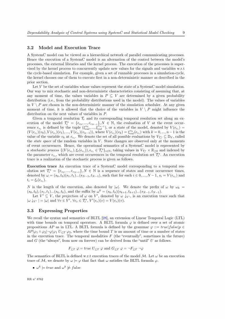
We consider here some examples of variables in V that represent the state of the simulationkernel and the SystemC model. A system state can consists of the information about all locationsbefore the execution of all statements that contain the devision operator “/” followed by zero ormore spaces and the variable “a” in a SystemC model (e.g., the statement y = (x + 1) / a).Let Producer and Consumer be two modules of a SystemC model. Assume that Producer has afunction send() and Consumer has a function receive(). Two variables send_start and send_donecan be defined as Boolean variables in V that hold the value true immediately before and aftera call of the function send(), respectively to express the status of the call stack. Similarly, thevariable rcv holds the value true immediately after a call of the function receive(). Assume againthat Producer has an event named write_event, to observe whenever this event is notified, wecan use a variable we_notified that holds the value true immediately when the event is notified.We will consider how these variables can be defined in our implementation of the verificationframework in the next section.

We have discussed so far the state of a SystemC model execution. It remains to discuss howthe semantics of the temporal operators is interpreted over the states in the execution of themodel. That means how the states are sampled. The following definition gives the concept oftemporal resolution, in which the states are evaluated only in instances in which the temporalresolution holds. It allows the user to set granularity of time.

Temporal resolution A temporal resolution Tr is a finite set of Boolean expressions definedover V which specifies when the set of variables V is evaluated.

Temporal resolution can be used to define a more fine-grained model of time than a coarse-grained one provided by a cycle-based simulation. We call the expressions in Tr temporal events.Whenever a temporal event is satisfied or the temporal event occurs, V is sampled. For example,assume that we want the set of variables to be sampled whenever at the end of simulation-cyclenotification or immediately after the event write_event is notified during a run of the model.Hence, we can define a temporal resolution as the following set Tr = {edc, we_notified}, whereedc and we_notified are Boolean expressions that have the value true whenever the kernel phaseis at the end of the simulation-cycle notification and the event write_event notified, respectively.

We denote the set of occurrences of temporal events from Tr along an execution of a SystemCmodel by T sr , called a temporal resolution set. The value of a variable v ∈ V at an eventoccurrence ec ∈ T sr is defined by a mapping ξvval : T sr → Dv. Hence, the state of the SystemCmodel at ec is defined by a tuple (ξv0val, ..., ξ

vn−1

val ).A mapping ξt : T sr → T is called a time event that identifies the simulation time at each oc-

currence of an event from the temporal resolution. Hence, the set of time points which correspondto a temporal resolution set T sr = {ec0 , ..., ecN−1

}, N ∈ N is given as follows.

Time tag Given a temporal resolution set T sr , the time tag T corresponding to T sr is a finiteor infinite set of non-negative reals {t0, t1, ..., tN−1}, where ti+1 − ti = δti ∈ R≥0, ti = ξt(eci).

Inria


3.2 Model and Execution TraceA SystemC model can be viewed as a hierarchical network of parallel communicating processes.Hence the execution of a SystemC model is an alternation of the control between the model’sprocesses, the external libraries and the kernel process. The execution of the processes is super-vised by the kernel process to concurrently update new values for the signals and variables w.r.tthe cycle-based simulation. For example, given a set of runnable processes in a simulation-cycle,the kernel chooses one of them to execute first in a non-deterministic manner as described in theprior section.

Let V be the set of variables whose values represent the state of a SystemC model simulation.Our way to mix stochastic and non-deterministic characteristics consisting of assuming that, atany moment of time, the values variables in P ⊆ V are determined by a given probabilitydistribution (i.e., from the probability distributions used in the model). The values of variablesin V \ P are chosen in the non-deterministic manner of the simulation scheduler. At any givenmoment of time, it is allowed that the choice of the variables in V \ P might influence thedistribution on the next values of variables in P .

Given a temporal resolution Tr and its corresponding temporal resolution set along an ex-ecution of the model T sr = {ec0 , ..., ecN−1

}, N ∈ N, the evaluation of V at the event occur-rence eci is defined by the tuple (ξv0val, ..., ξ

vn−1

val ), or a state of the model, denoted by V (eci) =(V (eci)(v0), V (eci)(v1), ..., V (eci)(vn−1)), where V (eci)(vk) = ξvkval(eci) with k = 0, ..., n−1 is thevalue of the variable vk at eci . We denote the set of all possible evaluations by VT s

r⊆ DV , called

the state space of the random variables in V . State changes are observed only at the momentsof event occurrences. Hence, the operational semantics of a SystemC model is represented bya stochastic process {(V (eci), ξt(eci)), eci ∈ T sr }i∈N, taking values in VT s

r× R≥0 and indexed by

the parameter eci , which are event occurrences in the temporal resolution set T sr . An executiontrace is a realization of the stochastic process is given as follows.

Execution trace An execution trace of a SystemC model corresponding to a temporal res-olution set T sr = {ec0 , ..., ecN−1

}, N ∈ N is a sequence of states and event occurrence times,denoted by ω = (s0, t0)(s1, t1)...(sN−1, tN−1), such that for each i ∈ 0, ..., N − 1, si = V (eci) andti = ξt(eci).

N is the length of the execution, also denoted by |ω|. We denote the prefix of ω by ωk =(s0, t0), (s1, t1)...(sk, tk), and the suffix by ωk = (sk, tk)(sk+1, tk+1)...(sN−1, tN−1).

Let V ′ ⊆ V , the projection of ω on V ′, denoted by ω ↓V ′ , is an execution trace such that|ω ↓V ′ | = |ω| and ∀v ∈ V ′, ∀ec ∈ T sr , V ′(ec)(v) = V (ec)(v).

3.3 Expressing PropertiesWe recall the syntax and semantics of BLTL [28], an extension of Linear Temporal Logic (LTL)with time bounds on temporal operators. A BLTL formula ϕ is defined over a set of atomicpropositions AP as in LTL. A BLTL formula is defined by the grammar ϕ ::= true|false|p ∈AP |ϕ1 ∧ϕ2|¬ϕ|ϕ1 U≤T ϕ2, where the time bound T is an amount of time or a number of statesin the execution trace. The temporal modalities F (the “eventually”, sometimes in the future)and G (the “always”, from now on forever) can be derived from the “until” U as follows.

F≤T ϕ = true U≤T ϕ and G≤T ϕ = ¬F≤T ¬ϕ

The semantics of BLTL is defined w.r.t execution traces of the modelM. Let ω be an executiontrace ofM, we denote by ω |= ϕ that fact that ω satisfies the BLTL formula ϕ.

• ωk |= true and ωk 6|= false

RR n° 8762

10 Ngo & Legay

• ωk |= p, p ∈ AP iff p ∈ L(sk), where L(sk) is the set of atomic propositions which are truein state sk

• ωk |= ϕ1 ∧ ϕ2 iff ωk |= ϕ1 and ωk |= ϕ2

• ωk |= ¬ϕ iff ωk 6|= ϕ

• ωk |= ϕ1 U≤T ϕ2 iff there exists an integer i such that ωk+i |= ϕ2, Σ0<j≤i(tk+j− tk+j−1) ≤T , and for each 0 ≤ j < i, ωk+j |= ϕ1

In our framework, the set of atomic proposition AP consists of the predicates defined over the setof variables V . Using these predicates, users can define temporal properties related to the stateof the kernel and the state of the SystemC model. Recall that Producer and Consumer are twoSystemC modules that have two functions send() and receive(), respectively. We consider thefollowing variables send_start, send_done and rcv ∈ V . They expose the state of the SystemCmodel as described in the section above. Assume that we want to express the property “over aperiod of T1 time units, send() remains blocked until receive() has returned within T2 time units”.This property can be specified with the “until” operator that is given as follows.

G≤T1(send_start→ (¬send_done U≤T2 rcv))

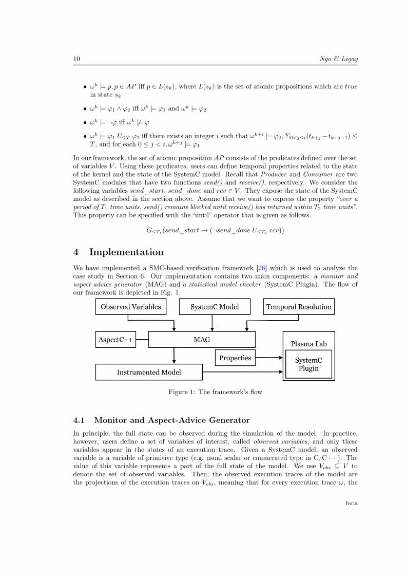
4 ImplementationWe have implemented a SMC-based verification framework [26] which is used to analyze thecase study in Section 6. Our implementation contains two main components: a monitor andaspect-advice generator (MAG) and a statistical model checker (SystemC Plugin). The flow ofour framework is depicted in Fig. 1.

Figure 1: The framework’s flow

4.1 Monitor and Aspect-Advice GeneratorIn principle, the full state can be observed during the simulation of the model. In practice,however, users define a set of variables of interest, called observed variables, and only thesevariables appear in the states of an execution trace. Given a SystemC model, an observedvariable is a variable of primitive type (e.g, usual scalar or enumerated type in C/C++). Thevalue of this variable represents a part of the full state of the model. We use Vobs ⊆ V todenote the set of observed variables. Then, the observed execution traces of the model arethe projections of the execution traces on Vobs, meaning that for every execution trace ω, the

Inria


corresponding observed execution trace is ω ↓Vobs. In the following, when we mention about

execution traces, we mean observed execution traces.The implementation of MAG allows users to define a set of observed variables that is used

with a temporal resolution to generate a monitor based on the techniques in [29] in order to makean instrumented SystemC model. The instrumented model will produce a set of execution tracesof the model. The generated monitor evaluates the set of observed variables at every time pointin which an event of the temporal resolution occurs during the SystemC model simulation. Thegenerator also generates an aspect-advice file that is used by AspectC++ [6] to automaticallyinstrument the SystemC model.

4.2 SystemC Plasma Lab PluginOur statistical model checker is implemented as a plugin of Plasma Lab [2] which establishesan interface between Plasma Lab and the instrumented model being executed by the simulator.In the current version, the communication is done via the standard input and output. Theplugin requests new states until the satisfaction of the formula to be verified can be decided,which terminates because the temporal operators are bounded. Similarly, depending on thehypothesis testing algorithms (e.g., sequential hypothesis testing, Monte Carlo simulation, or2-sided Chernoff bound), the plugin will request new traces from the instrumented model.

4.3 Running VerificationRunning the verification framework consists of two steps as follows. First, users define a set ofobserved variables and a temporal resolution in a configuration file, as well as other necessaryinformation. From that information, the generator generates the monitors and aspect-advicesthat are used by AspectC++ to produce the instrumented SystemC model. In addition, the gen-erator can automatically generate a Plasma Lab project file according to the desired properties.The instrumented model and the generated monitors are compiled together and linked with theSystemC simulation kernel into an executable model in order to make a set of execution traces ofthe system. In the second step, the plugin of Plasma Lab is used to verify the desired properties.The satisfaction checking of the properties is brought out based on the set of execution traces byexecuting the instrumented SystemC model and can be done by several hypothesis testing algo-rithms provided by Plasma Lab. The full implementation of our verification framework includingthe monitor and aspect-advice generator and the checker can be downloaded on the website ofPlasma Lab2.

5 Modeling Dependability in SystemCSHLPNs are high-level Petri nets (HLPNs) [24, 14, 21], in which each transition execution hasa duration described by an exponential distribution. They are commonly used for modelingdistributed systems in order to study their performance and dependability [8, 21, 20]. In thissection, we propose an approach for realizing SHLPNs in SystemC such that the semantics ispreserved.

5.1 Stochastic High-Level Petri NetsHigh-level Petri nets provide a compact representation of complex systems. There are manydifferent types of HLPNs that have been proposed in literature such as predicate transition

2MAG manual: https://project.inria.fr/plasma-lab/documentation/tutorial/mag_manual/

RR n° 8762

https://project.inria.fr/plasma-lab/documentation/tutorial/mag_manual/

12 Ngo & Legay

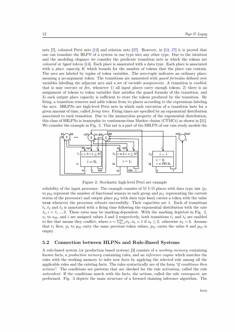
nets [7], coloured Petri nets [12] and relation nets [27]. However, in [13, 27] it is proved thatone can translate the HLPN of a system in one type into any other type. Due to the intuitionand the modeling elegance we consider the predicate transition nets in which the tokens arecoloured or typed tokens [14]. Each place is annotated with a data type. Each place is associatedwith a place capacity K which bounds for the number of tokens that the place can contain.The arcs are labeled by tuples of token variables. The zero-tuple indicates an ordinary place,meaning a no-argument token. The transitions are annotated with guard formulas defined overvariables labelling the adjacent arcs and a set of variable assignments. A transition is enabled,that is may execute or fire, whenever 1) all input places carry enough tokens, 2) there is anassignment of tokens to token variables that satisfies the guard formula of the transition, and3) each output place capacity is sufficient to store the tokens produced by the transition. Byfiring, a transition removes and adds tokens from/to places according to the expressions labelingthe arcs. SHLPNs are high-level Petri nets in which each execution of a transition lasts for agiven amount of time, called firing time. Firing times are specified by an exponential distributionassociated to each transition. Due to the memoryless property of the exponential distribution,this class of SHLPNs is isomorphic to continuous-time Markov chains (CTMCs) as shown in [21].We consider the example in Fig. 2. This net is a part of the SHLPN of our case study models the

Figure 2: Stochastic high-level Petri net example

reliability of the input processor. The example consists of 51 I/O places with data type int (p1to p50 represent the number of functional sensors in each group and p51 representing the currentstatus of the processor) and output place p52 with data type bool carries a token with the valuetrue whenever the processor reboots successfully. Their capacities are 1. Each of transitionst1, t2 and t3 is annotated with a firing time following the exponential distribution with the rateλi, i = 1, ..., 3. These rates may be marking-dependent. With the marking depicted in Fig. 2,s1 to s50, and i are assigned values 3 and 2 respectively, both transitions t1 and t2 are enabledto fire that means they conflict, where s = Σ50

k=1σk, σk = 1 if sk ≥ 2, otherwise σk = 0. Assumethat t1 fires, p1 to p50 carry the same previous token values, p51 caries the value 0 and p52 isempty.

5.2 Connection between HLPNs and Rule-Based Systems

A rule-based system (or production based system) [3] consists of a working memory containingknown facts, a production memory containing rules, and an inference engine which matches therules with the working memory to infer new facts by applying the selected rule among all theapplicable rules and the existing facts. The rules syntactically are of the form “if conditions thenactions”. The conditions are patterns that are checked for the rule activation, called the ruleantecedent. If the conditions match with the facts, the actions, called the rule consequent, areperformed. Fig. 3 depicts the main structure of a forward chaining inference algorithm. The

Inria


1 void Infer(working_memory ,production_memory) {

2 rules = Select(working_memory ,production_memory);

3 while(rules 6= ∅) {4 rule = SolveConflicts(rules);5 ApplyRule(rule);6 rules = Select(working_memory ,

production_memory);7 } //END while8 }

1 rule_set Select(working_memory ,production_memory) {

2 rules = ∅;3 for rule ∈ production_memory {4 if Match(rule ,working_memory)5 rules = rules ∪ rule;6 } //END for7 return rules;8 }

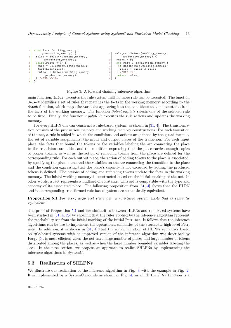
Figure 3: A forward chaining inference algorithmmain function, Infer, executes the rule system until no more rule can be executed. The functionSelect identifies a set of rules that matches the facts in the working memory, according to theMatch function, which maps the variables appearing into the conditions to some constants fromthe facts of the working memory. The function SolveConflicts selects one of the selected ruleto be fired. Finally, the function ApplyRule executes the rule actions and updates the workingmemory.

For every HLPN one can construct a rule-based system, as shown in [31, 4]. The transforma-tion consists of the production memory and working memory constructions. For each transitionof the net, a rule is added in which the conditions and actions are defined by the guard formula,the set of variable assignments, the input and output places of the transition. For each inputplace, the facts that bound the tokens to the variables labeling the arc connecting the placeto the transitions are added and the condition expressing that the place carries enough copiesof proper tokens, as well as the action of removing tokens from the place are defined for thecorresponding rule. For each output place, the action of adding tokens to the place is associated,by specifying the place name and the variables on the arc connecting the transition to the placeand the condition expressing that the place’s capacity is not exceeded by adding the producedtokens is defined. The actions of adding and removing tokens update the facts in the workingmemory. The initial working memory is constructed based on the initial marking of the net. Inother words, a fact represents a multiset of constants. This set is compatible with the type andcapacity of its associated place. The following proposition from [31, 4] shows that the HLPNand its corresponding transformed rule-based system are semantically equivalent.

Proposition 5.1 For every high-level Petri net, a rule-based system exists that is semanticequivalent.

The proof of Proposition 5.1 and the similarities between HLPNs and rule-based systems havebeen studied in [31, 4, 25] by showing that the rules applied by the inference algorithm representthe reachability set from the initial marking of the initial Petri net. It follows that the inferencealgorithms can be use to implement the operational semantics of the stochastic high-level Petrinets. In addition, it is shown in [31, 4] that the implementation of HLPNs semantics basedon rule-based systems with an improved version of the inference algorithm was described byForgy [5], is most efficient when the net have large number of places and large number of tokensdistributed among the places, as well as when the large number bounded variables labeling thearcs. In the next section, we propose an approach to realize SHLPNs by implementing theinference algorithms in SystemC.

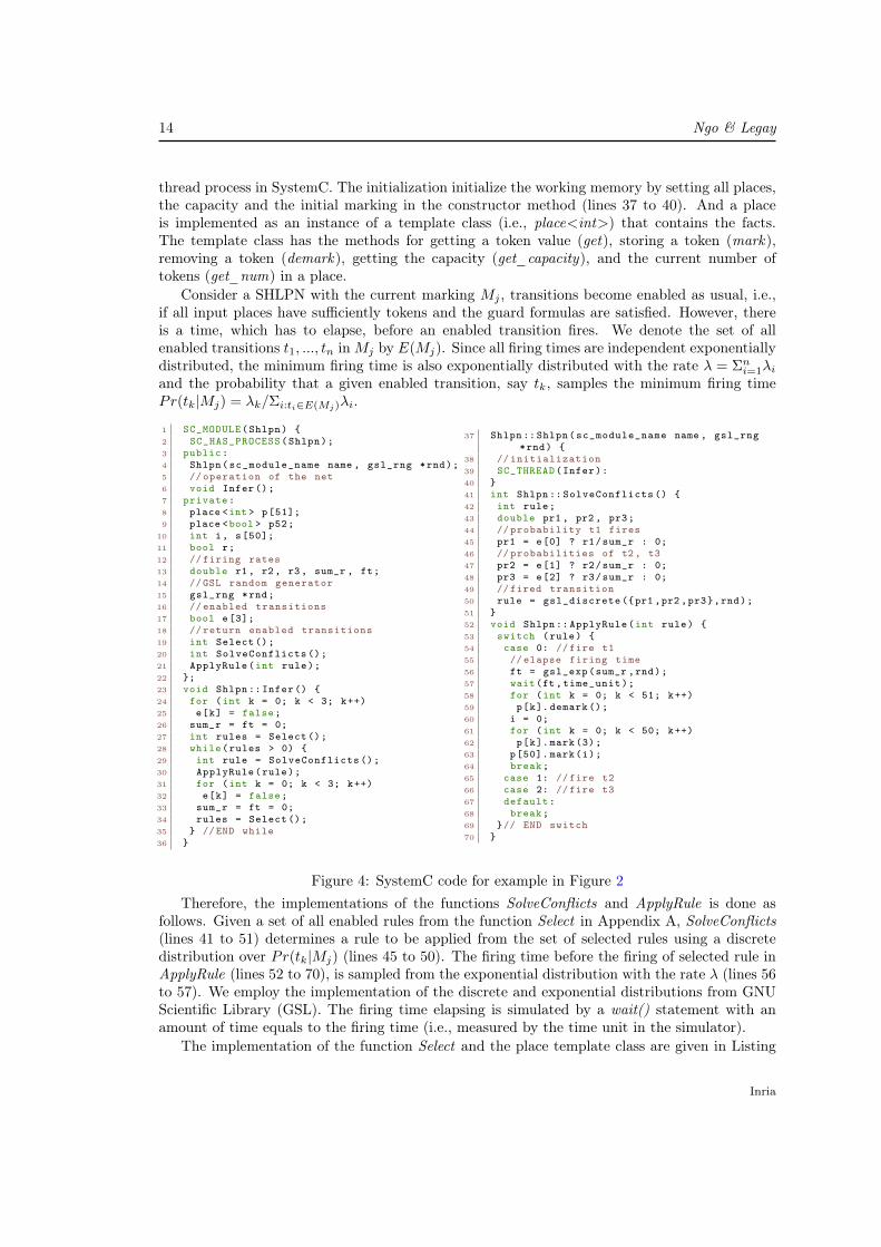
5.3 Realization of SHLPNsWe illustrate our realization of the inference algorithm in Fig. 3 with the example in Fig. 2.It is implemented by a SystemC module as shown in Fig. 4, in which the Infer function is a

RR n° 8762

14 Ngo & Legay

thread process in SystemC. The initialization initialize the working memory by setting all places,the capacity and the initial marking in the constructor method (lines 37 to 40). And a placeis implemented as an instance of a template class (i.e., place<int>) that contains the facts.The template class has the methods for getting a token value (get), storing a token (mark),removing a token (demark), getting the capacity (get_capacity), and the current number oftokens (get_num) in a place.

Consider a SHLPN with the current marking Mj , transitions become enabled as usual, i.e.,if all input places have sufficiently tokens and the guard formulas are satisfied. However, thereis a time, which has to elapse, before an enabled transition fires. We denote the set of allenabled transitions t1, ..., tn inMj by E(Mj). Since all firing times are independent exponentiallydistributed, the minimum firing time is also exponentially distributed with the rate λ = Σni=1λiand the probability that a given enabled transition, say tk, samples the minimum firing timePr(tk|Mj) = λk/Σi:ti∈E(Mj)λi.

1 SC_MODULE(Shlpn) {2 SC_HAS_PROCESS(Shlpn);3 public:4 Shlpn(sc_module_name name , gsl_rng *rnd);5 // operation of the net6 void Infer();7 private:8 place <int > p[51];9 place <bool > p52;

10 int i, s[50];11 bool r;12 // firing rates13 double r1, r2 , r3 , sum_r , ft;14 //GSL random generator15 gsl_rng *rnd;16 // enabled transitions17 bool e[3];18 // return enabled transitions19 int Select ();20 int SolveConflicts ();21 ApplyRule(int rule);22 };23 void Shlpn:: Infer() {24 for (int k = 0; k < 3; k++)25 e[k] = false;26 sum_r = ft = 0;27 int rules = Select ();28 while(rules > 0) {29 int rule = SolveConflicts ();30 ApplyRule(rule);31 for (int k = 0; k < 3; k++)32 e[k] = false;33 sum_r = ft = 0;34 rules = Select ();35 } //END while36 }

37 Shlpn :: Shlpn(sc_module_name name , gsl_rng*rnd) {

38 // initialization39 SC_THREAD(Infer):40 }41 int Shlpn :: SolveConflicts () {42 int rule;43 double pr1 , pr2 , pr3;44 // probability t1 fires45 pr1 = e[0] ? r1/sum_r : 0;46 // probabilities of t2 , t347 pr2 = e[1] ? r2/sum_r : 0;48 pr3 = e[2] ? r3/sum_r : 0;49 //fired transition50 rule = gsl_discrete ({pr1 ,pr2 ,pr3},rnd);51 }52 void Shlpn:: ApplyRule(int rule) {53 switch (rule) {54 case 0: //fire t155 // elapse firing time56 ft = gsl_exp(sum_r ,rnd);57 wait(ft,time_unit);58 for (int k = 0; k < 51; k++)59 p[k]. demark ();60 i = 0;61 for (int k = 0; k < 50; k++)62 p[k].mark (3);63 p[50]. mark(i);64 break;65 case 1: //fire t266 case 2: //fire t367 default:68 break;69 }// END switch70 }

Figure 4: SystemC code for example in Figure 2Therefore, the implementations of the functions SolveConflicts and ApplyRule is done as

follows. Given a set of all enabled rules from the function Select in Appendix A, SolveConflicts(lines 41 to 51) determines a rule to be applied from the set of selected rules using a discretedistribution over Pr(tk|Mj) (lines 45 to 50). The firing time before the firing of selected rule inApplyRule (lines 52 to 70), is sampled from the exponential distribution with the rate λ (lines 56to 57). We employ the implementation of the discrete and exponential distributions from GNUScientific Library (GSL). The firing time elapsing is simulated by a wait() statement with anamount of time equals to the firing time (i.e., measured by the time unit in the simulator).

The implementation of the function Select and the place template class are given in Listing

Inria


2 and Listing 3.

1 int Shlpn:: Select () {2 int s, rules = 0;3 bool check_p = true;4 //check t1 is enabled5 //check all input places have sufficiently tokens6 for(int k = 0; k < 50; k++) {7 if (p[k]->get_num () > 0)8 s[k] = p[k]->get();9 else {

10 check_p = false;11 break;12 }13 } //END for14 if (p[50]-> get_num () > 0)15 i = p[50]->get();16 else check_p = false;17 //check the guard formula18 if (check_p) {19 for (int k = 0; k < 50; k++)20 if (s[k] >= 2)21 s = s + 1;22 if (s >= 37 && i > 0) {23 //set t1 is enabled transition24 e[0] = true;25 sum_r = sum_r + r1;26 rules = rules + 1;27 } //END if28 } //END if29 //check t2 is enabled30 //check t3 is enabled31 return rules;32 }

Listing 2: SystemC code for the Select function

1 template <class type > class place {2 public:3 type get(int); //get token at index4 bool mark(type); // store token5 void demark(int); // delete token at index6 int get_capacity (); // place capacity7 int get_num (); // number of tokens8 };9

10 template <class type > type place <type >:: get(int index) {11 //code12 }1314 template <class type > bool place <type >:: mark(type t) {15 //code16 }

Listing 3: SystemC code for a place

6 Case Study and Results

In this section, our SystemC-realization is used to model the dependability of a large embeddedcontrol system. We also demonstrate the use of our verification framework to analyze the resultingmodel. The number of components in our system makes numerical approaches such as PMCunfeasible.

RR n° 8762

16 Ngo & Legay

6.1 An Embedded Control System

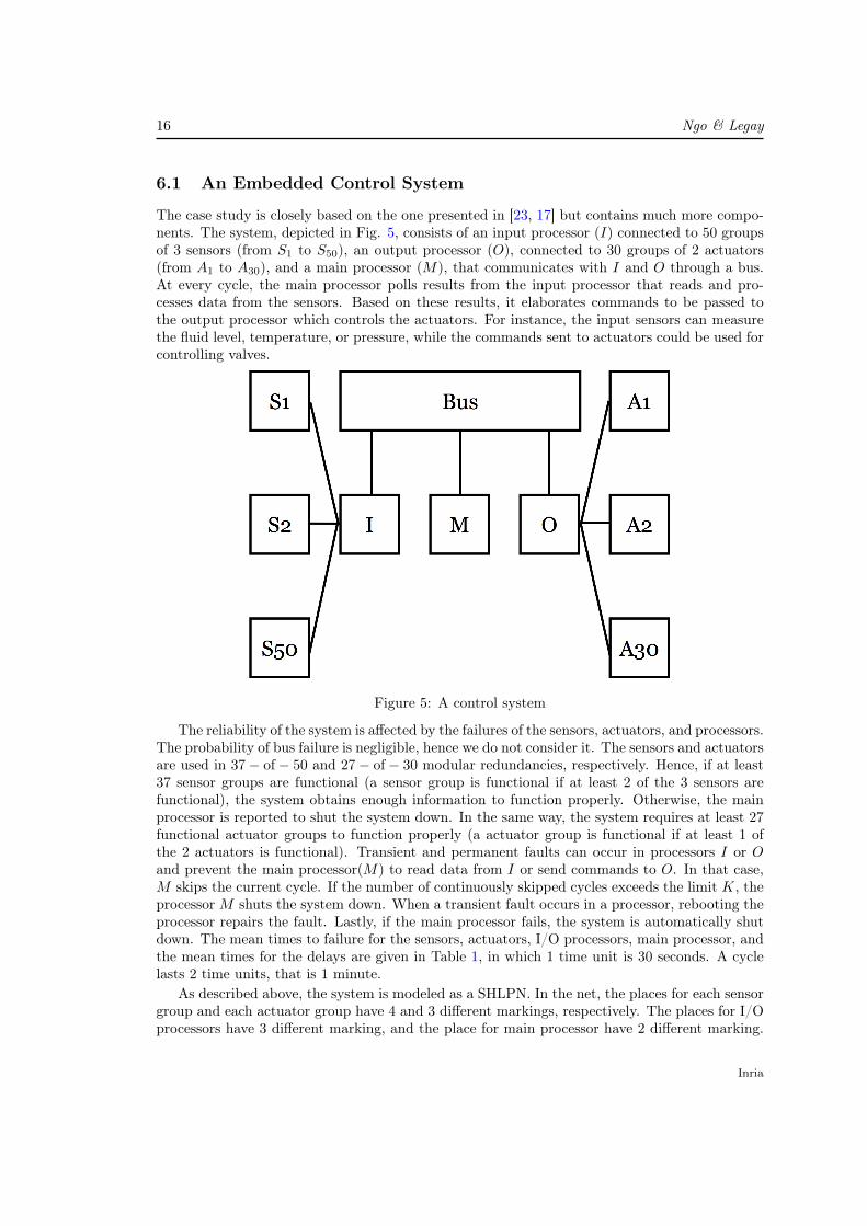
The case study is closely based on the one presented in [23, 17] but contains much more compo-nents. The system, depicted in Fig. 5, consists of an input processor (I) connected to 50 groupsof 3 sensors (from S1 to S50), an output processor (O), connected to 30 groups of 2 actuators(from A1 to A30), and a main processor (M), that communicates with I and O through a bus.At every cycle, the main processor polls results from the input processor that reads and pro-cesses data from the sensors. Based on these results, it elaborates commands to be passed tothe output processor which controls the actuators. For instance, the input sensors can measurethe fluid level, temperature, or pressure, while the commands sent to actuators could be used forcontrolling valves.

Figure 5: A control system

The reliability of the system is affected by the failures of the sensors, actuators, and processors.The probability of bus failure is negligible, hence we do not consider it. The sensors and actuatorsare used in 37− of− 50 and 27− of− 30 modular redundancies, respectively. Hence, if at least37 sensor groups are functional (a sensor group is functional if at least 2 of the 3 sensors arefunctional), the system obtains enough information to function properly. Otherwise, the mainprocessor is reported to shut the system down. In the same way, the system requires at least 27functional actuator groups to function properly (a actuator group is functional if at least 1 ofthe 2 actuators is functional). Transient and permanent faults can occur in processors I or Oand prevent the main processor(M) to read data from I or send commands to O. In that case,M skips the current cycle. If the number of continuously skipped cycles exceeds the limit K, theprocessor M shuts the system down. When a transient fault occurs in a processor, rebooting theprocessor repairs the fault. Lastly, if the main processor fails, the system is automatically shutdown. The mean times to failure for the sensors, actuators, I/O processors, main processor, andthe mean times for the delays are given in Table 1, in which 1 time unit is 30 seconds. A cyclelasts 2 time units, that is 1 minute.

As described above, the system is modeled as a SHLPN. In the net, the places for each sensorgroup and each actuator group have 4 and 3 different markings, respectively. The places for I/Oprocessors have 3 different marking, and the place for main processor have 2 different marking.

Inria


Therefore, the underlying CTMCs for the net has ∼ 2155 states comparing to the model in [17]with ∼ 210 states.

6.2 Analysis Results

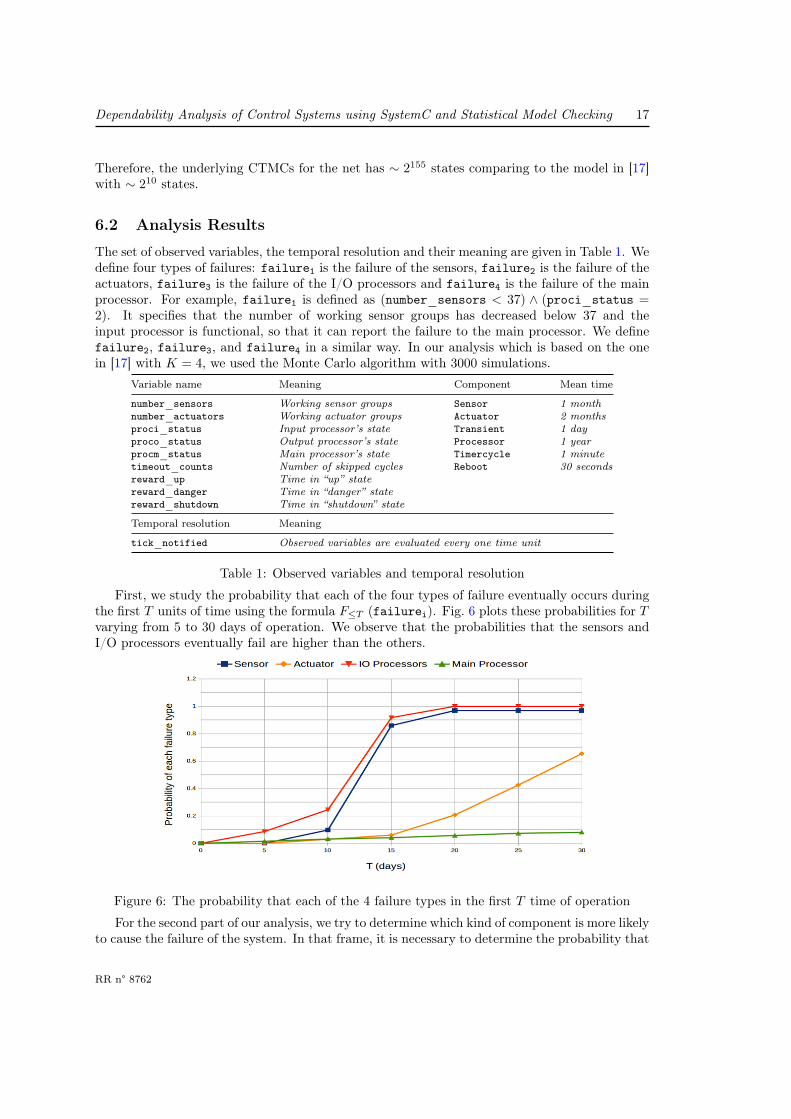
The set of observed variables, the temporal resolution and their meaning are given in Table 1. Wedefine four types of failures: failure1 is the failure of the sensors, failure2 is the failure of theactuators, failure3 is the failure of the I/O processors and failure4 is the failure of the mainprocessor. For example, failure1 is defined as (number_sensors < 37) ∧ (proci_status =2). It specifies that the number of working sensor groups has decreased below 37 and theinput processor is functional, so that it can report the failure to the main processor. We definefailure2, failure3, and failure4 in a similar way. In our analysis which is based on the onein [17] with K = 4, we used the Monte Carlo algorithm with 3000 simulations.

Variable name Meaning Component Mean time

number_sensors Working sensor groups Sensor 1 monthnumber_actuators Working actuator groups Actuator 2 monthsproci_status Input processor’s state Transient 1 dayproco_status Output processor’s state Processor 1 yearprocm_status Main processor’s state Timercycle 1 minutetimeout_counts Number of skipped cycles Reboot 30 secondsreward_up Time in “up” statereward_danger Time in “danger” statereward_shutdown Time in “shutdown” state

Temporal resolution Meaning

tick_notified Observed variables are evaluated every one time unit

Table 1: Observed variables and temporal resolution

First, we study the probability that each of the four types of failure eventually occurs duringthe first T units of time using the formula F≤T (failurei). Fig. 6 plots these probabilities for Tvarying from 5 to 30 days of operation. We observe that the probabilities that the sensors andI/O processors eventually fail are higher than the others.

Figure 6: The probability that each of the 4 failure types in the first T time of operation

For the second part of our analysis, we try to determine which kind of component is more likelyto cause the failure of the system. In that frame, it is necessary to determine the probability that

RR n° 8762

18 Ngo & Legay

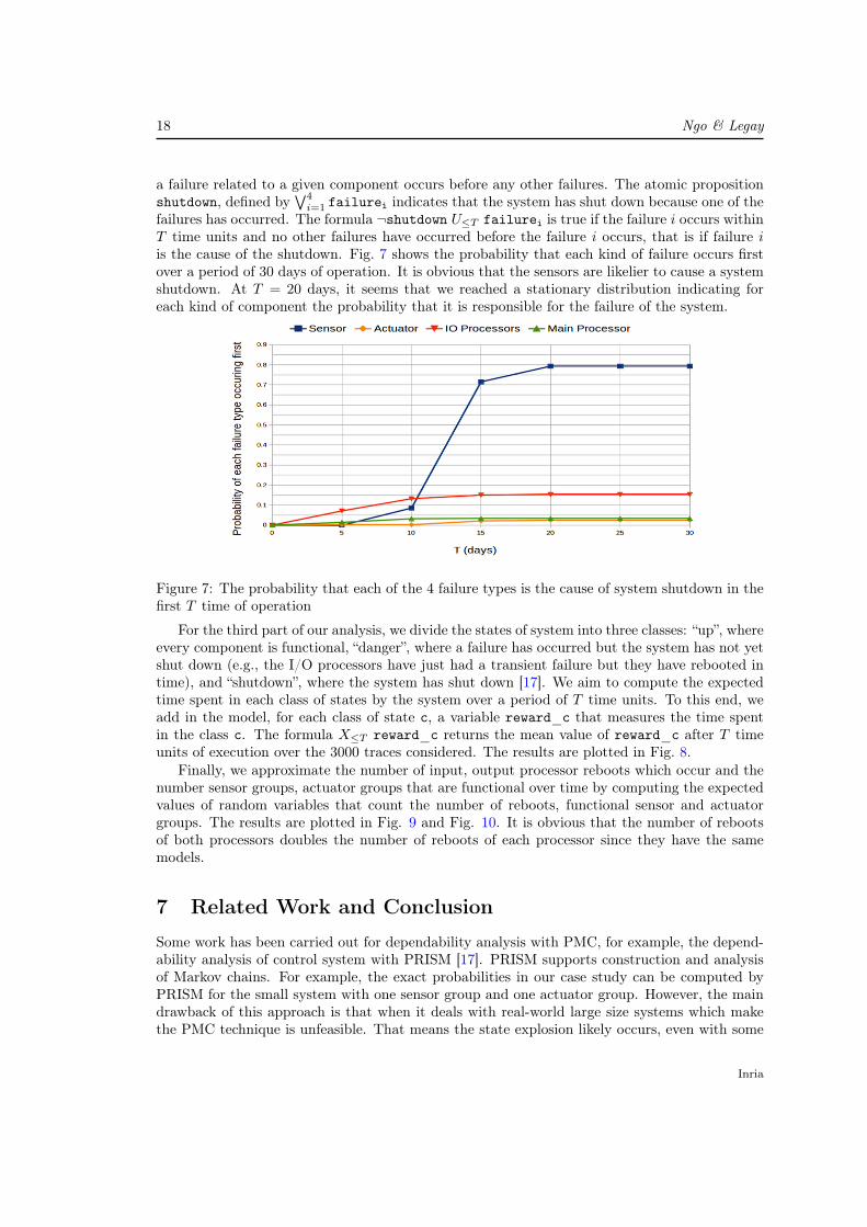
a failure related to a given component occurs before any other failures. The atomic propositionshutdown, defined by

∨4i=1 failurei indicates that the system has shut down because one of the

failures has occurred. The formula ¬shutdown U≤T failurei is true if the failure i occurs withinT time units and no other failures have occurred before the failure i occurs, that is if failure iis the cause of the shutdown. Fig. 7 shows the probability that each kind of failure occurs firstover a period of 30 days of operation. It is obvious that the sensors are likelier to cause a systemshutdown. At T = 20 days, it seems that we reached a stationary distribution indicating foreach kind of component the probability that it is responsible for the failure of the system.

Figure 7: The probability that each of the 4 failure types is the cause of system shutdown in thefirst T time of operation

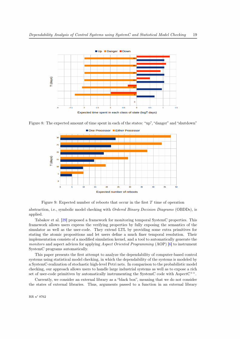
For the third part of our analysis, we divide the states of system into three classes: “up”, whereevery component is functional, “danger”, where a failure has occurred but the system has not yetshut down (e.g., the I/O processors have just had a transient failure but they have rebooted intime), and “shutdown”, where the system has shut down [17]. We aim to compute the expectedtime spent in each class of states by the system over a period of T time units. To this end, weadd in the model, for each class of state c, a variable reward_c that measures the time spentin the class c. The formula X≤T reward_c returns the mean value of reward_c after T timeunits of execution over the 3000 traces considered. The results are plotted in Fig. 8.

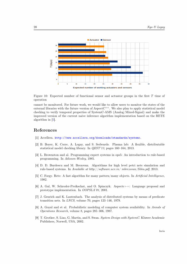
Finally, we approximate the number of input, output processor reboots which occur and thenumber sensor groups, actuator groups that are functional over time by computing the expectedvalues of random variables that count the number of reboots, functional sensor and actuatorgroups. The results are plotted in Fig. 9 and Fig. 10. It is obvious that the number of rebootsof both processors doubles the number of reboots of each processor since they have the samemodels.

7 Related Work and Conclusion

Some work has been carried out for dependability analysis with PMC, for example, the depend-ability analysis of control system with PRISM [17]. PRISM supports construction and analysisof Markov chains. For example, the exact probabilities in our case study can be computed byPRISM for the small system with one sensor group and one actuator group. However, the maindrawback of this approach is that when it deals with real-world large size systems which makethe PMC technique is unfeasible. That means the state explosion likely occurs, even with some

Inria


Figure 8: The expected amount of time spent in each of the states: “up”, “danger” and “shutdown”

Figure 9: Expected number of reboots that occur in the first T time of operation

abstraction, i.e., symbolic model checking with Ordered Binary Decision Diagrams (OBDDs), isapplied.

Tabakov et al. [29] proposed a framework for monitoring temporal SystemC properties. Thisframework allows users express the verifying properties by fully exposing the semantics of thesimulator as well as the user-code. They extend LTL by providing some extra primitives forstating the atomic propositions and let users define a much finer temporal resolution. Theirimplementation consists of a modified simulation kernel, and a tool to automatically generate themonitors and aspect advices for applying Aspect Oriented Programming (AOP) [6] to instrumentSystemC programs automatically.

This paper presents the first attempt to analyze the dependability of computer-based controlsystems using statistical model checking, in which the dependability of the systems is modeled bya SystemC-realization of stochastic high-level Petri nets. In comparison to the probabilistic modelchecking, our approach allows users to handle large industrial systems as well as to expose a richset of user-code primitives by automatically instrumenting the SystemC code with AspectC++.

Currently, we consider an external library as a “black box”, meaning that we do not considerthe states of external libraries. Thus, arguments passed to a function in an external library

RR n° 8762

20 Ngo & Legay

Figure 10: Expected number of functional sensor and actuator groups in the first T time ofoperation

cannot be monitored. For future work, we would like to allow users to monitor the states of theexternal libraries with the future version of AspectC++. We also plan to apply statistical modelchecking to verify temporal properties of SystemC-AMS (Analog/Mixed-Signal) and make theimproved version of the current naive inference algorithm implementation based on the RETEalgorithm in [5].

References

[1] Accellera. http://www.accellera.org/downloads/standards/systemc.

[2] B. Boyer, K. Corre, A. Legay, and S. Sedwards. Plasma lab: A flexible, distributablestatistical model checking library. In QEST’13, pages 160–164, 2013.

[3] L. Brownston and al. Programming expert systems in ops5: An introduction to rule-basedprogramming. In Adisson-Wesley, 1985.

[4] D. D. Burdescu and M. Brezovan. Algorithms for high level petri nets simulation andrule-based systems. In Available at http://software.ucv.ro/ mbrezovan/Sibiu.pdf, 2013.

[5] C. Forgy. Rete: A fast algorithm for many pattern/many objects. In Artificial Intelligence,1982.

[6] A. Gal, W. Schroder-Preikschat, and O. Spinczyk. Aspectc++: Language proposal andprototype implementation. In OOPSLA’01, 2001.

[7] J. Genrich and K. Lautenbach. The analysis of distributed systems by means of predicatetransition nets. In LNCS, volume 70, pages 123–146, 1979.

[8] A. Goyal and et al. Probabilistic modeling of computer system availability. In Annals ofOperations Research, volume 8, pages 285–306, 1987.

[9] T. Grotker, S. Liao, G. Martin, and S. Swan. System Design with SystemC. Kluwer AcademicPublishers, Norwell, USA, 2002.

Inria

http://www.accellera.org/downloads/standards/systemc


[10] H. Hermanns, B. Watcher, and L. Zhang. Probabilistic cegar. In CAV’08, volume 5123,pages 162–175. LNCS, Springer, 2008.

[11] A. Hinton, M. Kwiatkowska, G. Norman, and D. Parker. Prism: A tool for automaticverification of probabilistic systems. In TACAS’06, volume 3920, pages 441–444. LNCS,Springer, 2006.

[12] K. Jensen. Coloured petri nets and the invariant method. In Theoretical Comp. Sci.,volume 14, pages 317–336, 1981.

[13] K. Jensen. High-level petri nets. In Informatik-Fachberichte, volume 66, pages 166–180,1983.

[14] K. Jensen and L. Kristensen. Coloured petri nets: Modeling and validation of concurrentsystems. In Springer Verlag, 2009.

[15] S. Jha, E. Clarke, C. Langmead, A. Legay, A. Platzer, and P. Zuliani. A bayesian approachto model checking biological systems. In CMSB’09, volume 5688, pages 218–234. LNCS,Springer, 2009.

[16] J. Katoen, E. Hahn, H. Hermanns, D. Jansen, and I. Zapreev. The ins and outs of theprobabilistic model checker mrmc. In QEST’09. IEEE CS Press, 2009.

[17] M. Kwiatkowska, G. Norman, and D. Parker. Controller dependability analysis by proba-bilistic model checking. In Control Engineering Practice, volume 15(11), pages 1427–1434.Elsevier, 2007.

[18] A. Legay, B. Delahaye, and S. Bensalem. Statistical model checking: An overview. In RV’10,volume 6418, pages 122–135. LNCS, Springer, 2010.

[19] R. Lipsett, C. Schaefer, and C. Ussery. VHDL: Hardware description and design. KluwerAcademic Publishers, 1993.

[20] M. Marsan, G. Conte, and G. Balbo. A class of generalized stochastic petri nets for theperformance evaluation of multiprocessor systems. In ACM Trans. Comp. Systems, volume2(2), pages 93–122, 1984.

[21] M. Molloy. Performance analysis using stochastic petri nets. In IEEE Trans. Comp, volumeC-31(9), pages 913–917, 1982.

[22] W. Mueller, J. Ruf, D. Hoffmann, J. Gerlach, T. Kropf, and W. Rosenstiehl. The simulationsemantics of systemc. In DATE 2001, pages 64–70, 2001.

[23] J. Muppala, G. Ciardo, and K. Trivedi. Stochastic reward nets for reliability prediction. InCommunications in Reliability, Maintainability and Serviceability, volume 1(2), pages 9–20,1994.

[24] T. Murata. Petri nets: Properties, analysis and applications. In In Proceedings of the IEEE,volume 77(4), pages 541–580, 1989.

[25] T. Murata and D. Zhang. A predicate-transition net model for parallel interpretation oflogic programs. In IEEE Transactions on Software Engineering, volume 14(1), 1988.

[26] V. C. Ngo, A. Legay, and J. Quilbeuf. Dynamic verification of systemc with statistical modelchecking. In Research Report - RR-8644. INRIA Rennes - Bretagne Atlantique, ESTASYS,2014.

RR n° 8762

22 Ngo & Legay

[27] W. Reisig. Petri nets with individual tokens. In Informatik-Fachberichte, volume 66, pages229–249, 1983.

[28] K. Sen, M. Viswanathan, and G. Agha. On statistical model checking of stochastic systems.In CAV’05, volume 3576, pages 266–280. LNCS, Springer, 2004.

[29] D. Tabakov and M. Vardi. Monitoring temporal systemc properties. In Formal Methodsand Models for Codesign, pages 123–132. IEEE, 2010.

[30] D. Thomas and P. Moorby. The verilog hardware description language. In Springer. ISBN0-3878-4930-0, 2008.

[31] R. Valette and B. Bako. Software implementation of petri nets and compilation of rule-basedsystems. In Advances in Petri Nets, 1990.

[32] H. Younes. Ymer: A statistical model checker. In CAV’05, volume 3576, pages 429–433,2005.

Inria

RESEARCH CENTRERENNES – BRETAGNE ATLANTIQUE

Campus universitaire de Beaulieu35042 Rennes Cedex

PublisherInriaDomaine de Voluceau - RocquencourtBP 105 - 78153 Le Chesnay Cedexinria.fr

ISSN 0249-6399

dependability analysis of control systems using systemc and

Documents