department of physics, chemistry and biology - diva …647148/fulltext01.pdf · department of...

Department of Physics, Chemistry and Biology

Master’s Thesis in Applied Physics

A high sensitivity imaging detector for the study of theformation of (anti)hydrogen

Karl Berggren

LITH - IFM - A - EX - - 13/2827 - - SE

Research conducted at

CERN, Geneve, Switzerland

Department of Physics, Chemistry and BiologyLinkoping University

SE-581 83 Linkoping, Sweden

A high sensitivity imaging detector for the study of theformation of (anti)hydrogen

Department of Physics, Chemistry and Biology (IFM), Linkopings Universitet

Karl Berggren

LITH - IFM - A - EX - - 13/2827 - - SE

Thesis project: 30 hp

Supervisors: Dr. M. Doser,AEGIS, CERN

Dr. C. Hoglund,EES AB / Linkopings Universitet

Examiner: Dr. M. Magnusson,Linkopings Universitet

Linkoping: September 10, 2013

Datum 2013-09-10

Avdelning, institutionDivision, Department

Applied PhysicsDepartment of Physics, Chemistry and BiologyLinköping University

URL för elektronisk versionhttp://urn.kb.se/resolve?urn=urn:nbn:se:liu:diva-97359

ISBN

ISRN: LITH-IFM-A-EX--13/2827--SE_________________________________________________________________Serietitel och serienummer ISSNTitle of series, numbering ______________________________

SpråkLanguage

Svenska/Swedish

Engelska/English

________________

RapporttypReport category

Licentiatavhandling

Examensarbete

C-uppsats

D-uppsats

Övrig rapport

TitelA high sensitivity imaging detector for the study of the formation of (anti)hydrogen

FörfattareKarl Berggren

NyckelordCERN, AEGIS, MCP, Microchannel plates, cryo, cryogenic, antihydrogen, hydrogen, gain, resistance

SammanfattningAEGIS (Antimatter Experiment, Gravity, Interferometry and Spectroscopy) is an experiment under development at CERN which will measure earth's gravitational force on antimatter. This will be done by creating a horizontal pulsed beam of low energy antihydrogen, an atom consisting of an antiproton and a positron. The experiment will measure the vertical deflection of the beam through which it is possible to calculate the gravitational constant for antimatter. Tocharacterise the production process in the current state of the experiment it is necessary to develop an imaging detectorfor single excited hydrogen atoms. This thesis covers the design phase of that detector and includes studies and tests ofdetector components. Following literature studies, tests and having discarded several potential designs, a baseline design was chosen. The suggested detector will contain a set of ionising rings followed by an electron multiplying microchannel plate, a light emitting phosphor screen, a lens system and finally a CCD camera for readout. The detector will be able to detect single hydrogen atoms, measure their time of flight as well as being able to image electron plasmas and measure the time of flight of the initial particles in such a plasma. Tests were made to determine the behaviour of microchannel plates at the low temperatures used in the experiment. Especially, the resistance and multiplication factor of the microchannel plates have been measured at temperatures down to 14 K.

Abstract

AEGIS (Antimatter Experiment, Gravity, Interferometry and Spectroscopy) isan experiment under development at CERN which will measure earth’s gravi-tational force on antimatter. This will be done by creating a horizontal pulsedbeam of low energy antihydrogen, an atom consisting of an antiproton anda positron. The experiment will measure the vertical deflection of the beamthrough which it is possible to calculate the gravitational constant for antimat-ter. To characterise the production process in the current state of the experi-ment it is necessary to develop an imaging detector for single excited hydrogenatoms. This thesis covers the design phase of that detector and includes studiesand tests of detector components. Following literature studies, tests and havingdiscarded several potential designs, a baseline design was chosen. The suggesteddetector will contain a set of ionising rings followed by an electron multiplyingmicrochannel plate, a light emitting phosphor screen, a lens system and finallya CCD camera for readout. The detector will be able to detect single hydro-gen atoms, measure their time of flight as well as being able to image electronplasmas and measure the time of flight of the initial particles in such a plasma.Tests were made to determine the behaviour of microchannel plates at the lowtemperatures used in the experiment. Especially, the resistance and multipli-cation factor of the microchannel plates have been measured at temperaturesdown to 14 K.

Keywords: CERN, AEGIS, MCP, Microchannel plates, cryo, cryogenic, anti-hydrogen, hydrogen, gain, resistance

URL for electronic version:

http://urn.kb.se/resolve?urn=urn:nbn:se:liu:diva-97359

Abstract in Swedish: Sammanfattning

AEGIS (Antimatter Experiment, Gravity, Interferometry and Spectroscopy) arett experiment under uppbyggnad vid CERN som kommer att mata jordensgravitationella kraft pa antimateria. Detta kommer att goras genom att skapaen pulsad strale av antivate, en partikel som bestar av en antiproton och enpositron, och mata hur denna strale faller. Fran detta ar det sedan mojligt attberakna gravitationskonstanten for antimateria. For att karakterisera processenfor antivateproduktion behovdes en avbildande vatedetektor utvecklas for ex-

Berggren, 2013. vii

viii

perimentets kommissioneringsfas. Det har arbetet tacker designfasen av den de-tektorn och inkluderar studier och tester av detektorkomponenter. Efter litter-aturstudier, tester och ha eliminerat potentiella designkomponenter har ett de-signforslag tagits fram. Den foreslagna detektorn bestar av en grupp joniseranderingar foljt av elektronmultiplicerande mikrokanalplattor, en fluoroscerande fos-forskarm, ett linssystem och avslutas med en CCD kamera for utlasning. De-tektorn kommer kunna detektera enskilda vateatomer, mata deras flygtid ochaven avbilda elektronplasmor och mata flygtiden for de initiella partiklarna iett sadant plasma. Tester genomfordes for att bestamma mikrokanalplattor-nas egenskaper vid de laga temperatur som anvands i experimentet. Specielltsa har resistansen och multipliceringfaktorn for mikrokanalplattorna matts vidtemperaturer ner till 14 K.

Acknowledgements

It might be my thesis but this work couldn’t have been done with all the greatpeople I have around me such as. . .

. . . my mom and dad whom has always supported, encouraged and helped meto do whatever I wanted to do and do it well.

. . . my sister who I can talk to about anything between heaven and earth.

. . . my granddad who let me dissect all sorts of electronics when I was young,without him I would most certainly not be about to become an engineer.

. . . my university supervisor, Carina, who has been available to me on Skypeall the time, checked in on me regularly and even visited me at CERN.

. . . my examiner Martin, who has helped me with all the details that comeswith a master’s thesis and who also came and visited me.

. . . my supervisor at CERN, Michael. If I ever got lost in my work a talk withhim made everything so obvious and clear.

. . . Christian, who has helped me improve in all aspects of experimental physics.

. . . Andreas, who had great answers to both the good and the bad questions.

. . . all the other amazing people at AEGIS from whom I have learnt so much.

. . . my bros Olof and Rikard. Through the fires of Firenze and the frosts ofGeneve.

. . . all the great friends I’ve made here in Geneve, you make a good life great.

And lastly, thank you world for being such an awesome playground.

Berggren, 2013. ix

Nomenclature

The most important reoccurring abbreviations and symbols are described here.

Symbols

g Gravitational constant for antimatterε0 Vacuum permittivityεr Relative permittivityOAR Open Area Ratiop Protonp Antiprotone− Electrone+ PositronH HydrogenH AntihydrogenPs Positronium

Abbreviations

CERN European Center for Nuclear ResearchLHC Large Hadron ColliderAEGIS Antimatter Experiment Gravity, Inferferometry, SpectroscopyAD Antiproton DeceleratorMCP Microchannel plateSFC Segmented Faraday CupPSU Power Supply Unit

Berggren, 2013. xi

Contents

1 Introduction 11.1 Reading instructions . . . . . . . . . . . . . . . . . . . . . . . . . 11.2 CERN . . . . . . . . . . . . . . . . . . . . . . . . . . . . . . . . . 2

1.2.1 The LHC and the accelerator complex . . . . . . . . . . . 21.2.2 Experiments . . . . . . . . . . . . . . . . . . . . . . . . . 2

1.3 AEGIS . . . . . . . . . . . . . . . . . . . . . . . . . . . . . . . . . 51.4 The 1 T Penning trap . . . . . . . . . . . . . . . . . . . . . . . . 71.5 Purpose . . . . . . . . . . . . . . . . . . . . . . . . . . . . . . . . 10

2 Objective and layout of project 112.1 Initial state of development . . . . . . . . . . . . . . . . . . . . . 112.2 Objective . . . . . . . . . . . . . . . . . . . . . . . . . . . . . . . 12

2.2.1 Direct detection of Rydberg atoms . . . . . . . . . . . . . 132.2.2 Detection of ionised Rydberg atoms . . . . . . . . . . . . 132.2.3 Time of flight analysis of trapped electrons . . . . . . . . 132.2.4 Imaging of electron plasma distribution . . . . . . . . . . 13

2.3 Project layout . . . . . . . . . . . . . . . . . . . . . . . . . . . . . 14

3 Theory 153.1 Microchannel plates . . . . . . . . . . . . . . . . . . . . . . . . . 15

3.1.1 Electrical model . . . . . . . . . . . . . . . . . . . . . . . 173.1.2 Capacitance . . . . . . . . . . . . . . . . . . . . . . . . . . 183.1.3 Resistance . . . . . . . . . . . . . . . . . . . . . . . . . . . 183.1.4 Gain . . . . . . . . . . . . . . . . . . . . . . . . . . . . . . 193.1.5 Time constant of channels and full MCP . . . . . . . . . . 203.1.6 Dark counts . . . . . . . . . . . . . . . . . . . . . . . . . . 203.1.7 Detection efficiencies . . . . . . . . . . . . . . . . . . . . . 213.1.8 MCP gamma events . . . . . . . . . . . . . . . . . . . . . 233.1.9 Resolution . . . . . . . . . . . . . . . . . . . . . . . . . . . 243.1.10 Gain change in magnetic fields . . . . . . . . . . . . . . . 25

3.2 Phosphor screens . . . . . . . . . . . . . . . . . . . . . . . . . . . 25

4 Methods 274.1 First MCP low temperature test . . . . . . . . . . . . . . . . . . 27

4.1.1 Setup details . . . . . . . . . . . . . . . . . . . . . . . . . 274.1.2 Measurement complications . . . . . . . . . . . . . . . . . 304.1.3 Verifying bias difference for Faraday Cup . . . . . . . . . 304.1.4 Measuring resistance over MCP versus temperature . . . 30

Berggren, 2013. xiii

xiv Contents

4.1.5 Measuring MCP gain . . . . . . . . . . . . . . . . . . . . 324.1.6 Measuring event rate versus housing current . . . . . . . . 33

4.2 Room temperature tests . . . . . . . . . . . . . . . . . . . . . . . 334.2.1 Gain . . . . . . . . . . . . . . . . . . . . . . . . . . . . . . 334.2.2 Saturation . . . . . . . . . . . . . . . . . . . . . . . . . . . 334.2.3 Electron gun characterisation . . . . . . . . . . . . . . . . 34

4.3 Second MCP low temperature test . . . . . . . . . . . . . . . . . 344.3.1 Resistance . . . . . . . . . . . . . . . . . . . . . . . . . . . 344.3.2 Gain . . . . . . . . . . . . . . . . . . . . . . . . . . . . . . 354.3.3 Pulse tests . . . . . . . . . . . . . . . . . . . . . . . . . . 354.3.4 Recuperation time . . . . . . . . . . . . . . . . . . . . . . 35

4.4 Room temperature tests with optical readout . . . . . . . . . . . 354.4.1 Constant current saturation . . . . . . . . . . . . . . . . . 374.4.2 Pulsing . . . . . . . . . . . . . . . . . . . . . . . . . . . . 37

4.5 Methods used in analysis . . . . . . . . . . . . . . . . . . . . . . 384.5.1 Fitting . . . . . . . . . . . . . . . . . . . . . . . . . . . . . 384.5.2 Filtering data from temperature measurements . . . . . . 38

5 Measurement results and analysis 395.1 MCP Resistance . . . . . . . . . . . . . . . . . . . . . . . . . . . 395.2 MCP Gain . . . . . . . . . . . . . . . . . . . . . . . . . . . . . . 405.3 High rate behaviour . . . . . . . . . . . . . . . . . . . . . . . . . 40

5.3.1 Gain saturation at room temperature . . . . . . . . . . . 435.3.2 Constant current saturation . . . . . . . . . . . . . . . . . 43

5.4 Pulse behaviour . . . . . . . . . . . . . . . . . . . . . . . . . . . . 435.5 Time constant . . . . . . . . . . . . . . . . . . . . . . . . . . . . 455.6 Phosphor screen . . . . . . . . . . . . . . . . . . . . . . . . . . . 45

6 Discarded designs 476.1 Segmented Faraday Cup . . . . . . . . . . . . . . . . . . . . . . . 476.2 Delay Line Detector . . . . . . . . . . . . . . . . . . . . . . . . . 486.3 Direct electron detection using a CCD . . . . . . . . . . . . . . . 50

6.3.1 Image conduit . . . . . . . . . . . . . . . . . . . . . . . . 506.3.2 Camera in cryostat . . . . . . . . . . . . . . . . . . . . . . 50

7 Specification and design of chosen system 537.1 Microchannel plates . . . . . . . . . . . . . . . . . . . . . . . . . 537.2 Phosphor screen . . . . . . . . . . . . . . . . . . . . . . . . . . . 547.3 Lens system . . . . . . . . . . . . . . . . . . . . . . . . . . . . . . 547.4 Camera . . . . . . . . . . . . . . . . . . . . . . . . . . . . . . . . 54

8 Discussion 558.1 H* detection . . . . . . . . . . . . . . . . . . . . . . . . . . . . . 558.2 Plasma cloud imaging . . . . . . . . . . . . . . . . . . . . . . . . 568.3 Electron Time-Of-Flight . . . . . . . . . . . . . . . . . . . . . . . 568.4 Lowering γ noise . . . . . . . . . . . . . . . . . . . . . . . . . . . 568.5 Characterising detector and dark counts . . . . . . . . . . . . . . 578.6 Other MCP properties . . . . . . . . . . . . . . . . . . . . . . . . 578.7 Direct electron detection with CCD . . . . . . . . . . . . . . . . 588.8 Next steps . . . . . . . . . . . . . . . . . . . . . . . . . . . . . . . 58

Contents xv

A Explanation of additional concepts 59A.1 The Weak Equivalence Principle . . . . . . . . . . . . . . . . . . 59A.2 Penning traps . . . . . . . . . . . . . . . . . . . . . . . . . . . . . 59A.3 Rydberg atoms . . . . . . . . . . . . . . . . . . . . . . . . . . . . 61A.4 Stark acceleration . . . . . . . . . . . . . . . . . . . . . . . . . . 61

B Baseline design 63B.1 Ionising rings . . . . . . . . . . . . . . . . . . . . . . . . . . . . . 63B.2 MCP . . . . . . . . . . . . . . . . . . . . . . . . . . . . . . . . . . 63B.3 Phosphor . . . . . . . . . . . . . . . . . . . . . . . . . . . . . . . 65B.4 Lens system and camera . . . . . . . . . . . . . . . . . . . . . . . 65

B.4.1 Layout in AEGIS Apparatus . . . . . . . . . . . . . . . . 66B.4.2 Open issues and remarks . . . . . . . . . . . . . . . . . . 66

xvi Contents

Chapter 1

Introduction

The following chapter introduces the thesis, presenting the context of whereand why the detector is being developed. It starts out with an overview of thelayout of the thesis to simplify reading or finding particular information.

1.1 Reading instructions

This thesis was created to both represent the work done in the project as well asbeing a future reference for the AEGIS experiment. It therefore contains an ex-haustive method chapter as well as an appendix that summarises the importantdesign parameters that should be used in the continued development.

The current chapter introduces the project and the setting in which it has beenrun. It starts out describing the high level context of the project and thennarrows down to a level where the project parameters can be decided. Chapter2 further describes the project and defines the requirements for the end product.

Chapter 3 introduces relevant theory regarding microchannel plates (MCPs)and phosphor screens. Chapter 4 describes the methods used in tests and thedata analysis. Chapter 5 summarises and analyses the results from the tests.Chapter 6 presents the different design components that were not chosen forthe project and the reasons for not choosing them. Chapter 7 presents thechosen system and its specifications. Chapter 8 discusses the capabilities of thedesigned system as well as other topics of interest that were encountered duringthe project.

Appendix A explains different concepts that are important to the AEGIS exper-iment but not directly relevant to the work in this thesis. Appendix B containsa summary of the specifications for the system and is intended to be referencedocument for future work.

Berggren, 2013. 1

2 Chapter 1. Introduction

1.2 CERN

The European Organization for Nuclear Research (CERN) is the worlds largestphysics research institute; employing about 2400 people and hosting more than10,000 guest scientists from 608 different universities. It was founded in 1954by 12 European nations for research about the nucleus, the centre of atoms.The researchers at CERN were soon able to start probing deeper than just thenucleus and today they study even smaller constituents of matter, also making itknown as the European laboratory for particle physics. CERN is made up of andmainly financed by 20 member states but is also funded by financing agenciesfrom other countries and has cooperation agreements and scientific contactswith even more countries. The yearly budget is today over 1 billion CHF (7billion SEK) and it is mainly used for construction of the equipment needed forthe experiments such as accelerators, detectors and computing infrastructure.[1]

1.2.1 The LHC and the accelerator complex

The main workhorse at CERN at the moment is the LHC (Large Hadron Col-lider). The LHC is a circular particle accelerator with a circumference of 27 kmthat can accelerate either protons or heavy lead ions in two beams in oppositedirections. With up to 3.5 TeV per particle in each beam the resulting collisionshas a total energy of up to 7 TeV. The LHC cannot accelerate particles fromrest and the particles are therefore accelerated in stages in what is known as theaccelerator complex (Figure 1.1). The accelerator complex consists of severalaccelerators where the majority of them act as boosters for the LHC but theyare also used independently for other experiments. They also in a way reflectthe history of CERN as several of them have at some point been used as themain accelerator.

The LHC supplies the particle beams for the main experiments at CERN butthere are also other parts of the complex that serve other experiments. Ex-amples of these are the ISOLDE, the n-TOF and CNGS (CERN Neutrinos toGrand Sasso) targets, the CTF-3 (CLIC Test Facility) and the AD (AntiprotonDecelerator).

CTF-3 is a test facility for the next generation of linear colliders where newcomponents and techniques are being evaluated for one of the candidates toreplace the LHC after it’s decommissioning.

The AD decelerates antiprotons from close to the speed of light down to only10% of it. The antiprotons are used as a source for several experiments studyingthe properties of antimatter.

1.2.2 Experiments

ATLAS (A Toroidal LHC Apparatus) and CMS (Compact Muon Solenoid) arethe main experiments at CERN which are searching for new fundamental parti-cles by studying the high energy proton-proton collisions produced by the LHC.

1.2. CERN 3

Figure 1.1: (colour) An overview of the present accelerator complex at CERNand some of its experiments


They both have the same mission but are using two different designs for theirdetectors. This increases the chance of finding new particles as well as givingthe ability to double check each others results. The other two large LHC exper-iments are LHCb, which studies differences between matter and antimatter viathe bottom quark, and ALICE (A Large Ion Collider Experiment) where quark-gluon plasmas are studied, a state of matter that is thought to have existed justafter the big bang. There are also smaller experiments connected to the LHCas for example MOEDAL (Monopole and Exotics Detector at the LHC) whichis searching for the hypothetical magnetic monopoles.

There are also a number of non-LHC experiments, some of them make use ofother accelerators at CERN while some do not need accelerators at all. Thereare several experiments studying the standard model such as DIRAC (Dime-son Relativistic Atom Complex) which studies properties of the strong force viapionium decay. Beyond standard model experiments such as CAST (CERN Ax-ion Solar Telescope) and OSQAR (Optical Search for QED Vacuum Bifringence,Axions and Photon Regeneration) which both are searching for the hypotheticalaxion particle. ISOLDE (Isotope mass Separator On-Line facility) is a facilitywith dozens of small scale experiments in atomic physics. The multi-purposedetector AMS (Alpha Magnetic Spectrometer) is mounted on the InternationalSpace Station. There are also more applied experiments such CLOUD (Cos-mics Leaving OUtdoor Droplets) which is studying the effect of cosmic rays incloud formation and AWAKE (Proton Driven Plasma Wakefield AccelerationExperiment) which is developing next-generation accelerator technology.

The AD complex hosts a range of experiments that are exploring the propertiesof antimatter by using the low energy antiprotons provided by the antipro-ton decelerator. The AD takes antiprotons from a metal target where proton-antiproton pairs are created in high energy collisions created by the PositronSynchrotron. These antiprotons are then slowed down in the decelerator fromseveral GeV down to MeV levels by using electron and stochastic cooling. Thecooled antiprotons are then distributed in bunches to the different experimentsin the AD complex. The current experiments working in the AD complex are

• ACE (Antiproton Cell Experiment) is studying how antiprotons affecthuman cells and its suitability as a future cancer therapy.

• ALPHA captures and studies antihydrogen and compares it to ordinaryhydrogen.

• ASACUSA (Atomic Spectroscopy And Collisions Using Slow Antiprotons)is studying antimatter by creating hybrid particles such as ”antiprotonichelium”. These hybrid atoms have longer lifetimes than antihydrogen andcan therefore be studied in further extent.

• ATRAP also studies antihydrogen but is using different techniques, suchas cold positron cooling, to try to capture the antihydrogen for longertimes.

• The AEGIS (Antihydrogen Experiment: Gravity, Interferometry, Spec-troscopy) experiment is studying the gravitational force on antimatter.This thesis covers work that is part of the development of the AEGISexperiment.

1.3. AEGIS 5

The Higgs boson

One of the best current models for describing our universe is called the StandardModel. It describes three of the four forces in nature, the electromagnetic, thestrong and the weak force. The model can be seen as describing the world bythe interaction of a set of fundamental particles and these particles make upthe universe as we know it, with energy, matter and the forces that connecteverything. Until recently, all particles in the Standard Model except one hadbeen observed, the Higgs boson. Named after the man who predicted it, ithad been haunting particle physicists for several years and was one of the mainreasons for the construction of the LHC. The Higgs boson is a key elementof the Standard Model since it is the particle that gives other particles mass.Understanding the origin of mass is an essential factor in a successful theoryfor understanding our universe. In the summer of 2012 the ATLAS and CMSexperiments announced together that they had both discovered a particle witha rest-energy of 126 GeV, which is in the predicted mass range and also withother properties compatible with the ones predicted for the Higgs boson. Thisparticle is today considered to be the Higgs boson but there are still questionsregarding its properties. Therefore ATLAS and CMS continue to study theHiggs boson at the same time as the next generation of accelerators are beingdesigned, that will be able to study the Higgs with even higher precision.

Long Shutdown 1

The accelerator complex at CERN is currently shut down for upgrades, theupgrade period being called Long Shutdown 1. After this time the LHC willbe able to produce collisons with energies up to 14 TeV compared to the max-imum of 8 TeV reached in 2012. The interval between collisions will also bereduced from 50 ns to 25 ns. At the same time upgrades are being done at theantiproton decelerator, specifically an additional cooling ring is being installednamed ELENA. This ring will be able to cool antiprotons even further, reducingthe need for degrader foils at which a large portion of the flux is lost otherwise.ELENA will also in contrast to the previous ejector be able to deliver antiprotonbunches simultaneously to all experiments, allowing for increased beam time andextended data collection. With the addition of increased beam time, AEGIS isalso expected to increase its event rate ten-fold when ELENA starts operatingin 2017.[2]

1.3 AEGIS

The AEGIS experiment at CERN seeks to test the weak equivalence principle(WEP1) for anti-matter. This is to be done by creating a beam of cold (read:slow-moving) anti-hydrogen which is sent through a moire deflectometer2. This

1The weak equivalence principle is, in its essence, the principle that objects with the samestarting position and velocity will follow the identical trajectories in a gravitational fieldregardless of their mass and composition.

2A moire deflectometer consists of two gratings placed after each other and which createsa diffraction pattern from an impinging particle beam. Depending on the weight of the


Figure 1.2: (colour) Schematic images over the basic principle of the AEGISexperiment. Image: AEGIS/CERN

results in a diffraction pattern which can be used to measure the drop of thebeam due to gravity, which in turn tells us the earths gravitational force onanti-matter. According to the standard model this should be the same as forordinary matter but it has never been measured with sufficient precision andis thus an important step in strengthening the support for the WEP. However,a different gravitational force on antimatter would be a major discovery. Itcould for example help us explain the unbalanced ratio between matter andantimatter in the universe and would force the physics community to reevaluatethe standard model. [3][4]

To measure the gravitational fall of antihydrogen the following steps will bedone, as also illustrated in Figure 1.2.

• First antiprotons (p) coming from the AD are trapped and cooled to 100mK in a cylindrical Penning trap3.

• Shortly after, a beam of positrons (e+) will hit a nano-porous material justabove the trap. In this material the positrons will combine with electronsand form positronium (Ps)

e+ + e− → Ps.

The positronium ejects from the material in the direction of the antiprotontrap.

• To increase their lifetime, the positronium is excited, Ps → Ps∗, using alaser system focused in the region between the positronium converter andthe antiproton trap.

• The excited positronium is combined with antiprotons, creating excitedantihydrogen atoms and free electrons

p + Ps∗ → H∗

+ e−

particles they will fall a different distance between the two grates. This difference gives riseto a displaced diffraction pattern and by measuring the displacement of the pattern one candeduce the gravitational force on the particles.

3A Penning trap is set of electric and magnetic fields which together are able to confinecharged particles to a limited volume

1.4. The 1 T Penning trap 7

• The antihydrogen is accelerated into a beam using Stark acceleration,inhomogeneous electric fields that utilise the Stark shift4 in the atoms.The low temperature of the formed antihydrogen is essential to get a wellaligned beam since thermal velocities will cause radial divergence of theatoms.

• The beam goes through a moire deflectometer which creates a shifteddiffraction pattern depending on the fall of the particles. From this it ispossible to calculate the gravitational constant for the antihydrogen.

During the current Long Shutdown 1 the AEGIS experiment does not haveaccess to the antiprotons required to create antihydrogen. To keep the devel-opment going the experiment will instead perform measurements on regularhydrogen. This is possible due the symmetry in the process used to createthe antihydrogen. Changing the antiprotons to protons in the above reaction,hydrogen and a positron are formed instead

p + Ps∗ → H∗ + e+

A new complication arise from this: hydrogen, being ordinary matter, does notinteract as strongly with its surroundings as an antihydrogen atom would. Thereis therefore a need for a detector which can detect single excited hydrogen atomsand help characterise the processes that will be used to produce antihydrogen.This thesis covers part of the development of that detector. From here onthe contents of the thesis will mainly be discussed in regards to the hydrogenproduction.

1.4 The 1 T Penning trap

The main events of the experiment, the positronium and hydrogen production,will take place in a 1 T Penning trap located in the second half of the experimentchamber (see Figure 1.3 and Figure 1.4). This part of the experiment is sur-rounded by a superconducting solenoid which creates a homogeneous magneticfield of 1 T inside itself. The transition temperature for the superconductingmaterial, 7 K for 5 T magnet and 9 K for the 1 T magnet, is one of the reasonswhy the experiment is cooled to 4 K by using liquid helium. The other reason isthe importance of reducing the thermal velocities of the hydrogen and the 4 Kenvironment is then necessary to be able to cool the hydrogen in the trap downto the required 100 mK.

Inside the trap the protons will be trapped just below the positronium con-verter. Between the target and trap is the focus of the lasers that will excite thepositronium and in turn the hydrogen. The trap is constructed as a cylinderconsisting of several rings which can be biased at different potentials to controlthe trapping and eventually also accelerate the formed hydrogen. To reduce anynoise from stray particles, the inside of the chamber is also kept at ultra highvacuum with a pressure lower than 10−9 mbar and the trap will locally havea pressure down to 10−15 mbar. The trap ends approximately 4 cm from thecentre of the hydrogen formation region. From there there is 75 cm available

4The fine splitting of electron energy levels in electric fields due to their spin


A-A ( 1 : 10 )

A

A

1

1

2

2

3

3

4

4

5

5

6

6

A A

B B

C C

D D

A31T Magnet2.0.idw

1 Tolerances ISO2768 mKISO13920 BF

surface: N/A

N/A

Ra Ra

undimensioned edges ISO 13715surface DIN EN ISO 1302

Quantity:

material:

scale:creator: C. Loefflerdate: 04/09/2012checked by:date:

1T Magnet2.0PART NUMBER

State Changes Date Name

1T Magnet2.0.iam

middle plane

850

152,08532,5

150

Ø

125

Ø

360,95

936,2

Figure 1.3: Drawing of the 1 T magnet of the experiment and its interior,showing the 1 T trap in the centre and to the left the space in which thehydrogen detector will be placed. The 5 T magnet and the antiproton injectionis then placed to the right in the drawing and the moire deflectometer will beplaced to the left of the drawing. Image: AEGIS/CERN

1.4. The 1 T Penning trap 9

A-A ( 1 : 20 )

B ( 1 / 5 )

A

A

B

1

1

2

2

3

3

4

4

5

5

6

6

A A

B B

C C

D D

A3Drawing_space.idw

1 Tolerances ISO2768 mKISO13920 BF

surface: N/A

N/A

Ra Ra

undimensioned edges ISO 13715surface DIN EN ISO 1302

Quantity:

material:

scale:creator: C. Loefflerdate: 19.01.2013checked by:date:

Experiment MountedPART NUMBER

State Changes Date Name

Experiment Mounted.iam

125

150

377,35 294,5582,75

66

,5

Figure 1.4: A close up of the 1 T Penning trap (to the right in the drawing)and the region where the hydrogen detector will be placed. The centre of theimage shows the 66.5 mm restriction. Image: AEGIS/CERN


to the end of magnet with a 66.5 mm restriction in between (see Figure 1.4).It is within this space that the hydrogen detector will need to be placed in thecoming commissioning stages of the experiment.

1.5 Purpose

This thesis is a part of the development of a hydrogen detector for the AEGISexperiment that will be part of the commissioning process of the experiment.The final detector will be used to evaluate and characterise the hydrogen pro-duction of the experiment as a step towards the antihydrogen production thatwill start when the AD starts operating again in the second half of 2014. Withantihydrogen the AEGIS experiment will measure the gravitational force on an-timatter to help us increase our understanding about antimatter and possiblyexplain mysteries as for example the baryon asymmetry.

The master’s thesis is also a practical and theoretical learning experience whereprevious education is applied to solve new problems and new knowledge has tobe taken on to complement the existing.

Chapter 2

Objective and layout ofproject

The following chapter presents the state of the development at the start of theproject and general and use-case specific requirements for the detector. It isconcluded with an overview of how the project was structured and performed.

2.1 Initial state of development

Upon the start of this thesis there had already been some development doneregarding the hydrogen detector, mainly with respect to the initial ionisingstage and tests of a microchannel plate (MCP) delay line detector.

The principle of detection had at this point been decided to work by ionisingthe Rydberg hydrogen1 coming out of the 1 T Penning trap. This is done byplacing a set of rings with a high potential difference close to each other. At highenough electric field gradients this can ionise excited hydrogen atoms, allowingtheir constituents to be more easily controlled and accelerated. The lifetimeof the excited states is not exactly known in the conditions of the experimentbut is judged to at least be in the order of 100µs and possibly even longer.Nevertheless, due to the atoms low speed (coming from a sub-K region), it isstill important for the ionising rings to be as close as possible to the trap butwithout disturbing the sensitive processes taking place inside it. With a ringdesign one gets a radial dependence of the ionised states and if imaged preciselyenough it is considered possible to measure the distribution of the excited states.The ionising rings were also researched and developed further in parallel withthe development of the rest of the detector. [5]

1A Rydberg atom (also explained in Appendix A.3) is an atom with a high quantumnumber and with energy levels that are well described by the Bohr model

Berggren, 2013. 11

12 Chapter 2. Objective and layout of project

2.2 Objective

The objective of the project was to design and develop a detector that couldanalyse the hydrogen production in the AEGIS experiment. The process isthe same as the one that will be used when the experiment starts producingantihydrogen after Long Shutdown 1 and understanding its characteristics is animportant part of developing the experiment as a whole.

The requirements can be divided into general requirements about the detector,due to the environment it is supposed to operate in, and in four main use cases.The general requirements on the detector were as follows

• It must work in a 4 K environment and output little or no heat to itssurroundings. This is so that the device does not interfere with the sub-Kregions in the 1 T trap and that it has a minimal load on the cryogenicsystem of the experiment.

• It should also be able to handle temperature cycling up to 600 K to allowfor vacuum baking. Vacuum baking is a process of heating componentsto make them release molecules attached to their surfaces (mainly H2O).This is crucial to reach the vacuum levels required in the AEGIS experi-ment.

• It must work in a 1 T magnetic field. The 1 T magnetic field is an essentialpart of the Penning trap and the detector must be placed within the samemagnet.

• It must work in a ultra high vacuum, between 10−15 mbar and 10−9 mbar.The vacuum is necessary to keep unwanted elements out of the processand several different components also requires a high vacuum to operate.

• It must fit in the AEGIS experiment chamber and has to be easy to mount.The space inside the 1 T magnet is limited and this must be taken intoconsideration.

• The development and material costs should be kept within the budget ofthe experiment.

The properties that are to be studied with the detector is the hydrogen pro-duction rate and the characteristics of that hydrogen. The main characteristicof interest is the temperature of the hydrogen since it will have a strong ef-fect on the collimation of the atom beam. Another interesting characteristic isthe principle quantum number of the hydrogen which affects both the dipolemomentum of the hydrogen (which is important for the Stark acceleration, seeAppendix A.4) as well as the lifetime of the excited state. The use cases pre-sented below represent different measurements that will be done at differentstages in the production. They are here presented in their chronological orderin the experiment.

2.2. Objective 13

2.2.1 Direct detection of Rydberg atoms

The first use case is to directly detect Rydberg atoms without the use of theionising rings. The ionising rings will not be able to ionise all the excited statesand is expected to reach an ionisation rate of 25% for the n = 18 state[5]. It istherefore of interest to try to detect any hydrogen that has passed through thefirst stage of the detector. The main requirements for this are that

• The stage after the ionising rings should also be able to ionise more deeplybound Rydberg hydrogen to some degree.

• The detector should be able to detect single particles at a rate in the orderof 10 atoms in the time span of 10 µs to 1 ms after the hydrogen productionpulse. This is the approximate rate at which the experiment expectsto produce hydrogen in the beginning minus the approximate number ofatoms ionised.

• The events should preferably be timed but not necessarily matched withthe imaged particles. The time of arrival gives the time of flight which inturn can be used to calculate the velocity of the particles and thus also beused to estimate their temperature.

2.2.2 Detection of ionised Rydberg atoms

In the current design of the ionising rings it will be possible to trap the electronsfrom the hydrogen ionisation. This gives the possibility to delay the arrival ofthese electrons and do a separate measurement from that of the un-ionisedhydrogen. This requires the expected signal in the order of 20 electrons to bedetected simultaneously after being released from the trap. Since they havebeen delayed, the arrival times of single particles is not as interesting as in thefirst case.

2.2.3 Time of flight analysis of trapped electrons

Once the hydrogen production is done there will be surplus electrons/positronsfrom one of the antiproton/proton cooling mechanisms inside the trap, these canbe used to further analyse the production process and the environment it takesplace in. The temperature of these electrons can be measured by slowly lettingthem out of the trap and then measuring the distribution in the time of flightof these electrons. To do this the detector needs to be able to precisely measurethe arrival time of the first arriving particles with an exponentially increasingnumber of arrivals (with an expected total of 108 electrons). No imaging of theparticles is required for the time of flight measurement.

2.2.4 Imaging of electron plasma distribution

Another property to analyse is the spatial distribution of the electron plasma.This requires a spatial resolution that can distinguish 0.1 mm details and that

14 Chapter 2. Objective and layout of project

the equipment can handle the rate of 108 electrons within a time down to 100ns.

2.3 Project layout

From these requirements the possible options needed to be investigated andresearched. The project started out by evaluating several different technolo-gies where the main part of them was discarded for different reasons. Thesetechnologies are discussed in Chapter 6. The evaluation then resulted in a can-didate system which needed to be investigated further, the main concern beingthe performance of MCPs at low temperature and high rates. The main topiccovered in this thesis is the tests and analysis needed to understand the MCPperformance in the setting of the experiment. In addition to this the othercomponents that were decided upon after the evaluation phase, the phosphorscreen and optical readout, are also discussed.

Chapter 3

Theory

This chapter presents relevant theory for the project, it mainly covers the prin-ciples of different components and also discusses different models. The chaptermainly covers microchannel plates and phosphor screens.

Microchannel plates and phosphor screens are commonly used components inparticle detection and imaging. Both require additional hardware to create acomplete detector and they can also be used together as part of a detector.The microchannel plate is a highly grained electron multiplier which behind itrequires some sort of imaging device, either purely electrical by using for examplea delay line detector or segmented Faraday cup, or by electron-photon conversionusing a phosphor screen and then a regular camera readout. The phosphorscreen acts as mentioned as an electron to photon converter and requires somesort of imaging device after it such as a CCD or photographic plate. With acorrect setup the microchannel plate is able to multiply single particles whilethe phosphor screen requires several energetic electrons to produce enough lightfor imaging. However, together they can be used for single particle detectionand imaging with high accuracy.

3.1 Microchannel plates

The microchannel plate (MCP) is a fine grained electron multiplying devicewhich can be used for particle detectors with high spatial resolution. The prin-ciple of operation is schematically shown in Figure 3.1.

The multiplication process start with an impinging ionising particle, e.g. anelectron, ion or photon, having enough enough kinetic energy to liberate one ormore electrons from the wall of one of the MCPs channels. This impact releaseselectrons from the surface which are then accelerated by an electric field whichis induced by applying a high voltage difference over the MCP. The acceleratedelectrons knock out more electrons from the channel walls; creating an avalancheof electrons which is then emitted from the back of the MCP. The gain factor(number of electrons emitted for each incoming particle) is usually in the rangeof 103 to 105 for a single MCP. This factor can be increased by stacking multiple

Berggren, 2013. 15

16 Chapter 3. Theory

Figure 3.1: A schematic picture of the structure of a MCP and its principle ofoperation. The channels are usually slightly angled from the perpendicular ofthe MCP to prevent particles from passing straight through. Image: Hama-matsu Photonics K.K.

3.1. Microchannel plates 17

MCPs on each other. The gain increase is, however, not linear to the number ofMCPs but the method is known to be effective for stacks of up to three MCPs.

There are several manufacturing methods for making MCPs, one method asspecified in [6] is based on creating hexagonal arrays of microfibers which inturn can be fused together to larger sizes. These arrays of fibers are then cutat a slight angle, 8 to 15, to give the channel bias angle. Afterwards theplate goes through different process to lower the work function of the channelsurfaces. Lastly, the front and back of the plate are coated in a metal alloy tomake the surfaces conducting and to improve detection efficiency. The maindifferences between different brands of MCPs are the materials used in thebulk of the plate, the surface coatings and the final processing method of thechannel walls resulting in different work functions. It is also possible to improvethe performance in certain applications by making thicker MCPs (for gammadetection) or applying different types of surface coatings (for example for X-raydetection).

Each channel is in the order of 2 − 25 µm in diameter and has a length todiameter ratio, L/d, in the order of 40 to 80 for standard MCPs. L/d andthe secondary emission factor of the material inside the channel are the mainfactors that determine the gain of the MCP [6]. Since it is the L/d factor thataffects the gain one can produce MCPs with smaller channel diameter whilemaintaining the same gain. This is relevant for extended dynamic range MCPs,which have smaller channel diameters to be able to handle larger input signals.The small channel diameter of MCPs gives a high position resolution makingthem a good choice in several high sensitivity imaging applications. Examplesof these are camera sensors with high demands on low-light sensitivity such ashigh-speed or night-vision cameras.

3.1.1 Electrical model

One simple, yet effective, method of modelling an MCP considers each channelas an RC-circuit as was done by Fraser et. al. [7]. Characterising each channelwith Rch and Cch the time constant of the system will be τch = kRchCch wherek is constant. Analysing this structure one also finds that the time constantmust be same as the time constant of the entire MCP, τMCP = τch.

Using some assumptions regarding the gain and operation of the MCP, Fraserarrives at the equation

IpIs

=Gc(0)MRMCP /V01N + kRMCPCMCP

where Ip is the output current, Is is the strip current, Gc(0) is the charge gain forlow count rates, M is the number of channels, V0 is the applied voltage and N isthe count rate. This equation shows the saturation behaviour of the MCP, theratio between the output pulse and the strip current of the MCP is limited forhigh rates. This means that a MCP with a limited current supply can at mostoutput pulses corresponding to a certain fraction of the total current throughthe MCP. Hamamatsu [8] specifies this maximum ratio to approximately 7%.


3.1.2 Capacitance

One of the important properties of the MCP is the capacitance. It influencesthe RC time constant of the MCP but it can also be used to estimate the totalcharge available in a channel. Measuring the capacitance is usually complicateddue to other capacitances affecting the measuring circuit and calculating it isusually precise enough and more consistent when comparing different MCPs.

The capacitance of a MCP can be approximately calculated using a parallelplate capacitor model [7]

CMCP = ε0(εr(1− aopen) + aopen)AMCP

L

where ε0 is the vacuum permittivity, εr is the relative permittivity of the glassused, aopen is the open area ratio, AMCP is the area of the MCP and L is thethickness. This formula assumes that the whole MCP is active, i.e. coveredwith channels. However, most MCPs have an additional rim not containing anychannels but with the conductive coating. To calculate the capacitance of aMCP with a rim, the above expression has to be modified slightly by addingthe capacitance of the rim (since it can be considered to be a parallel coupledcapacitance).

CMCP = ε0(εr(1− aopen) + aopen)AactiveL

+ ε0εrArimL

Since the MCPs used in this report are circular it is more convenient to usethe total MCP diameter, dMCP , and active diameter, dactive, which are wellspecified properties.

CMCP = ε0(εr(1− aopen) + aopen)πd2active

4L+ ε0εr

π(d2MCP − d2active)4L

Using the values for a Hamamatsu F1217-01 and estimating the relative permit-tivity of the glass to be that of lead glass we arrive at at a total capacitance ofapproximately 300 pF, where the contribution from the active area is approxi-mately 150 pF, i.e. half of the total capacitance.

3.1.3 Resistance

There are three main materials that contribute to the resistivity of a MCP; theinsulating bulk glass, the conductive surface coating and the semiconductingsurface of the channels. The two surfaces can be considered as two resistancescoupled in series around the parallel coupled bulk and channel coating. Dueto the well insulating properties of the lead-glass in the bulk and the relativelyhigh conductivity of the surfaces the MCP will mainly get its resistance be-haviour from the channel walls and thus behave as a semiconductor in termsof conductivity. The nature of semiconductors also determines the temperaturedependence of the resistivity. Since the conductive properties of a semiconduc-tor mainly come from thermally excited electrons that move to the valence bandthe resistance should scale with the Boltzmann factor, eε/kT . This gives semi-conductors an exponentially increasing resistance as the temperature decreasesand at 0 K it is essentially a perfect insulator.


Earlier studies of MCPs by Roth and Fraser [9] suggest that there are regimeswith different dominating conduction mechanisms which can be modelled usingdifferent model parameters. Still assuming that the resistance is dependent onthe number of occupied states one can refine the previous suggested model byintroducing different activation energies, ε, for different intervals of T . The databy Roth and Fraser suggests two different regimes giving a piecewise resistancefunction

R(T ) =

R1e

ε1/kT , T ≤ T0R2e

ε2/kT , T > T0

with the restriction that the function is continuous.

3.1.4 Gain

The gain is the number of particles that are emitted for one electron beingreleased from the wall at the beginning of the channel and it is one of the mostimportant properties of a MCP. For single particle detection it is important thatthis number is high enough to generate sufficiently strong signals to be read outby standard electronics. It is therefore also essential to understand how the gainchanges with temperature. The gain mainly depends on the channel width tolength ratio, bias voltage, work function of the surface and the charge availablein the channel.

Schecker et al. [10] has developed a rate and temperature dependent gain modelstarting from a previous model

G = (κEc)n

where κ is a constant, Ec the collisional energy of electrons to the channel walland n is the number of stages (cascades) down a channel, giving the averagegain κEc per stage. Without consideration of rate and temperature this modelcan be written as

G = (κV0n

)n

where the parameters Ec =V 20

4α2ε and n = 4α2εV0

have been derived in earlierpapers. α is the length to diameter ratio and ε is the electron energy whenreleased from the wall.

To model the rate dependence the authors assume that the main charge deple-tion occurs in the last multiplication stage in the channel and that the charge inthis stage has a capacitive recharge. The multiplication factor of the last stageis replaced as κEc → κEc(1 − e−dt/τ ) where dt is the average time betweenevents and τ is the recharge time constant. This yields the new gain function

G = (κV0n

)n(1− e−dt/τ )

where a rate dependence has been introduced via dt and a temperature viaτ since we have τ = RchCch and Rch is a strongly temperature dependentfunction. An important property from this model is, as long as we assume thatthere is no or only very weak temperature dependence in κ and n, that the lowrate gain, dt→∞, is temperature independent.


3.1.5 Time constant of channels and full MCP

To account for differences between the time constant of a perfect RC-circuit,τ = RC and the actual time constant Fraser [7] introduces an additional factorsuch that τ = kτch = kRchCch. k is an MCP dependent factor and τch can beconsidered the natural RC time constant of the channel. Fraser assumes thatthe MCP can be considered an array of parallel RC circuits representing eachchannel, and under this assumption the natural time constant of an individualchannel is equal to the time constant of the whole MCP. However, this doesnot take into account the non-active area of the MCP which mainly gives riseto additional capacitance for the entire MCP rather than affecting individualchannels. Adding another capacitance, Crim, for the rim of the MCP yieldsτch = RMCP (CMCP − Crim), i.e. it is the capacitance of the active area thatdetermines the channel time constant. This should be taken into considerationwhen determining or predicting the time constant of a MCP. One cannot directlyuse the time constant of the MCP in an electrical circuit as the time constantof individual channels. The time constant of the entire MCP is for examplerelevant when considering fast bias changes in a MCP system and the channelconstant strongly affects the high rate behaviour of the MCP.

3.1.6 Dark counts

Undesired signals, known as dark counts, can stem from from residual ions inthe vacuum (external) or, more commonly, from thermally emitted electrons(internal) from the MCP. The MCPs used in this report are manufactured byHamamatsu Photonics K.K. and the internal dark counts are specified to belower than 3 Hz/cm2 giving that the total dark counts should be lower than42 Hz with the currently used MCP (F1217-01) [8]. The specified dark countrate comes from several factors which can cause the MCP channels to fire bythem self. An internal source of dark counts not accounted for in this number isthe ion back-scattering, which can arise at high bias voltages. The effect comesfrom positive ions being knocked out, accelerated backwards in the channel andhitting the channel wall at a point close to entry, causing a new cascade inthe channel. Electrically these events can be discerned from their pulse profile,giving a characteristic double peak. Using only a time-integrated image, as theone from a phosphor screen, this is much harder.

External dark counts can originate from radiation and gas as well as mechanicaldisturbances. MCPs are sensitive to UV-light, X-rays and gamma radiation,even though the detection efficiencies for these are considerably lower than forcharged or heavy particles. They are still a noteworthy source of noise, especiallyin the AEGIS experiment since the hydrogen production utilises UV-lasers andthere is 511 keV gamma radiation from the positronium decay. Alpha and betaradiation are clearly detectable by the MCP but in its operating environmentthere are no such sources and this should not cause a problem. Cosmic raysshould in theory be detectable as well but are negligible due to their low rates.Sporadic gas molecules which ionise in the MCP channel can also be a sourceof noise, however, the ultra high vacuum and low temperature used in theexperiment chamber reduces this source of noise considerably.


100

50

20

10

5

2

1

DE

TE

CT

ION

EF

FIC

IEN

CY

(%

)

ELECTRON ENERGY (keV)

0.05 0.1 0.2 0.5 1 2 5 100.02 20 50

RE

LAT

IVE

DE

TE

CT

ION

EF

FIC

IEN

CY

(a.

u.)

PHOTON ENERGY (keV)

0.1 1.0 10 1000

0.5

1.0

Figure 3.2: These two graphs show the non-trivial energy dependence on thedetection efficiency. Electrons to the left and photons in the UV and X-rayrange to the right. Image: Hamamatsu Photonics K.K.

3.1.7 Detection efficiencies

For non-charged massive particles the detection efficiency is clearly proportionalto the open area ratio but also depends on factors such as kinetic energy, po-tential to ionise in the MCP, etc. For charged particles the detection efficiencydepends on the electric field in and around the MCP, since the field lines cancreep into the channels when there is a bias difference over the MCP.

In the case of detecting electrons and photons there are several different ef-fects that influence the detection efficiency. For electrons, for example, higherenergies will make the electrons penetrate deeper into the bulk before transfer-ring their energy. Du to this, the secondary electrons are more likely to stopin the bulk rather than escaping the surface. For photons there are differentphenomena through which energy can be transferred to electrons, for examplethe photoelectric effect, Thomson scattering and Compton scattering. Thatthe detection efficiencies are non-linear with respect to the particles energies isalso illustrated in Figure 3.2. The figure shows the detection efficiencies energydependency for electrons and photons in selected ranges.

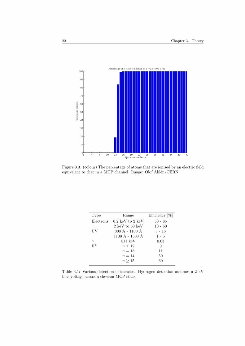
In the experiment it is also of interest to be able to detect Rydberg hydrogenatoms (i.e. excited hydrogen). Hydrogen normally requires very high electricfields to be ionised but the required field is significantly lower for excited states.Figure 3.3 shows how likely different states are to ionise in a 2 MV/m electricfield which is the strength of the field inside a channel at full gain settings.However, since the particles are neutral they are not guided by the electricor magnetic field and the chance of a hydrogen atom entering a channel isapproximately equal to the open area ratio of the MCP, 60%.

The efficiencies for relevant sources are summarised in Table 3.1.7.


1 4 7 10 13 16 19 22 25 28 31 34 37 400

10

20

30

40

50

60

70

80

90

100Percentage of n-state ionization in F =2.0e+06 V/m

Quantum number n

Percentageionized

Figure 3.3: (colour) The percentage of atoms that are ionised by an electric fieldequivalent to that in a MCP channel. Image: Olof Ahlen/CERN

Type Range Efficiency [%]

Electrons 0.2 keV to 2 keV 50 - 852 keV to 50 keV 10 - 60

UV 300 A - 1100 A 5 - 151100 A - 1500 A 1 - 5

γ 511 keV 0.03H* n ≤ 12 0

n = 13 11n = 14 50n ≥ 15 60

Table 3.1: Various detection efficiencies. Hydrogen detection assumes a 2 kVbias voltage across a chevron MCP stack


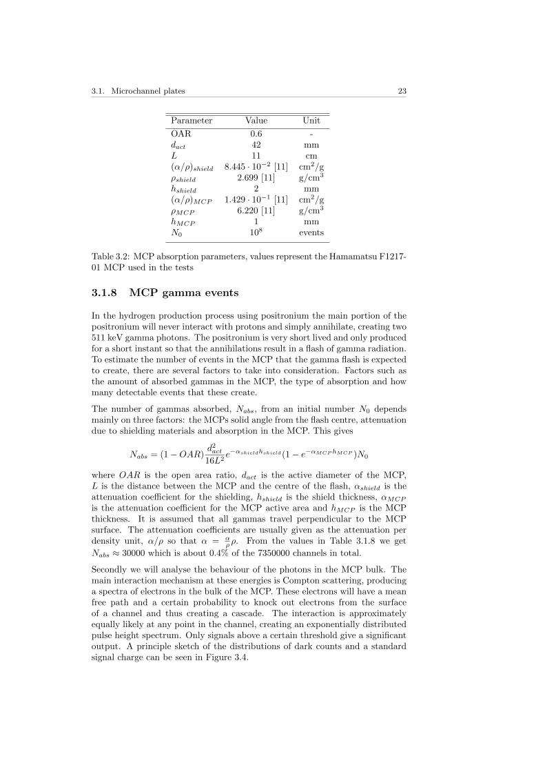
Parameter Value Unit

OAR 0.6 -dact 42 mmL 11 cm(α/ρ)shield 8.445 · 10−2 [11] cm2/gρshield 2.699 [11] g/cm3

hshield 2 mm(α/ρ)MCP 1.429 · 10−1 [11] cm2/gρMCP 6.220 [11] g/cm3

hMCP 1 mmN0 108 events

Table 3.2: MCP absorption parameters, values represent the Hamamatsu F1217-01 MCP used in the tests

3.1.8 MCP gamma events

In the hydrogen production process using positronium the main portion of thepositronium will never interact with protons and simply annihilate, creating two511 keV gamma photons. The positronium is very short lived and only producedfor a short instant so that the annihilations result in a flash of gamma radiation.To estimate the number of events in the MCP that the gamma flash is expectedto create, there are several factors to take into consideration. Factors such asthe amount of absorbed gammas in the MCP, the type of absorption and howmany detectable events that these create.

The number of gammas absorbed, Nabs, from an initial number N0 dependsmainly on three factors: the MCPs solid angle from the flash centre, attenuationdue to shielding materials and absorption in the MCP. This gives

Nabs = (1−OAR)d2act16L2

e−αshieldhshield(1− e−αMCPhMCP )N0

where OAR is the open area ratio, dact is the active diameter of the MCP,L is the distance between the MCP and the centre of the flash, αshield is theattenuation coefficient for the shielding, hshield is the shield thickness, αMCP

is the attenuation coefficient for the MCP active area and hMCP is the MCPthickness. It is assumed that all gammas travel perpendicular to the MCPsurface. The attenuation coefficients are usually given as the attenuation perdensity unit, α/ρ so that α = α

ρ ρ. From the values in Table 3.1.8 we get

Nabs ≈ 30000 which is about 0.4% of the 7350000 channels in total.

Secondly we will analyse the behaviour of the photons in the MCP bulk. Themain interaction mechanism at these energies is Compton scattering, producinga spectra of electrons in the bulk of the MCP. These electrons will have a meanfree path and a certain probability to knock out electrons from the surfaceof a channel and thus creating a cascade. The interaction is approximatelyequally likely at any point in the channel, creating an exponentially distributedpulse height spectrum. Only signals above a certain threshold give a significantoutput. A principle sketch of the distributions of dark counts and a standardsignal charge can be seen in Figure 3.4.


Number of events

Pulse charge [C]Detection treshold

Figure 3.4: (colour) The charge spectrum from dark counts will be exponentiallydistributed (blue) in comparison to the gaussian distribution of a proper signal(red).

The maximum electron energy, the Compton edge, is given by

ECompton =2E2

mec2 + 2E

Since the photon energy comes from an electron/positron annihilation the en-ergy is the same as the rest energy for an electron, giving ECompton = 2/3 ·mec

2 = 341 keV.

Using the NIST ESTAR data resource, the continuous slowing down approxima-tion range of 350 keV electrons is calculated to be 290 µm, which is significantlylonger than the channel pitch and one can therefore assume that most of theabsorbed photons will create a channel event.

Nevertheless, the interactions are equally distributed throughout the channeland therefore only a fraction create events that give signals that look like non-photon events. An estimation of the region that creates indistinguishable signalsis the visible depth (looking straight at a channel) which for a 12 µm channelwith a 8 angle is 85 µm. Compared to the full length of channels in a chevronstack, 1 mm, this is 8.5%. A rough estimate is then that approximately 10%,3000, of the absorbed gammas could be mistaken as hydrogen events.

3.1.9 Resolution

The resolution (size of discernible details) of the MCP is mainly determined byits channel pitch, which is 15 µm for the relevant MCPs.

3.2. Phosphor screens 25

The spread of light in the phosphor screen can be approximated by the contin-uous slowing down approximation range in phosphor which for 1 keV electronsis in the order of 1 µm, much lower than the size of the electron cloud from theMCP (which is at least 12 µm).

With the camera placed 170 mm from the last lens and a field of view of 70,each pixel covers approximately 230 µm. The camera resolution is the clearbottleneck of the system and actually gives a slightly worse resolution thanspecified in the requirements. Nevertheless it is within the right order and theperformance loss is acceptable.

3.1.10 Gain change in magnetic fields

It is clear that strong magnetic fields have an impact on the behaviour of MCPs.This has been previously studied by Schecker et al. [10] and is also known byMCP manufacturers [8] which conclude that it is possible to operate MCPsin magnetic fields but with some restrictions. The main restrictions are thestrength and orientation of the magnetic field compared to the MCP. Magneticfields with non-perpendicular components compared to the MCPs surface willseverely lower the gain of the MCP even at low field strengths. However, axiallyoriented fields, as is the case in the AEGIS experiment, can actually increasethe gain up to a certain point. The properties of the MCPs used in the studyby Schecker et al are similar to the ones used in this study and they found thatat a 1 T axial field the gain is approximately the same as without a magneticfield. This suggests that any gain change due to magnetic fields in the AEGISexperiment should be minimal as long as the MCPs are placed with their surfaceperpendicular to the magnetic field lines.

3.2 Phosphor screens

Phosphor screens are commonly used for imaging charged particles. They con-sist of a phosphor covered glass plate with a metal coating on top, usuallyaluminium or indium-tin-oxide. By accelerating the electrons enough (to about1 keV) they can pass through the 250 − 500 A thick aluminium layer and in-teract with the phosphor. The electrons give rise to photo-luminescence in thephosphor; exciting electrons to levels above the conduction band. These non-radiatively relax to the conduction band of the phosphor and then radiativelyrelax into their ground state, emitting photons with a wavelength correspondingto the band gap. The kinetic excitation from the impinging electrons indicatesthat the output light is approximately linear (above a threshold) to both thenumber of incoming electrons and their energy. Aluminium is a common choicedue to its reflective properties, allowing photons emitted back towards the anodeto be reflected and thereby increasing the total light emitted.

Chapter 4

Methods

This section covers the methods used in the different parts of the project. In par-ticular, this section covers the different test setups used and how measurementswere done.

The chapter is divided into five parts, the first four covering the main testsand the fifth covering the data analysis. The main test setups are presentedin chronological order: first cryogenic measurements, measurements at roomtemperature using the same setup, second cryogenic measurements using a newsetup, and room temperature tests with an optical readout added to the newsetup.

4.1 First MCP low temperature test

To test the behaviour of MCPs at low temperatures a basic test setup wasconstructed and mounted to a cryocooler. In principle, as illustrated in Figure4.1, the setup consists of an electron source that illuminates an area with knownsize on the MCP. The electrons are then multiplied in the MCP and emitted onto a Faraday cup from which the signal can be read out. The final setup usedin the cryotests can be seen in Figure 4.2.

4.1.1 Setup details

The setup consisted of the following components

• Chevron stack of Hamamatsu F1217-01 MCPs.

• Faraday cup made from a cleaned copper coated circuit board.

• Electron gun, Kimball Physics ES-015 BaO-coated disc cathode.

• 22Ω heating resistor.

• Cernox temperature sensor.

Berggren, 2013. 27

28 Chapter 4. Methods

Al-screen with Ø2 mm hole

Electron gun

Double stack MCPFaraday Cup

Figure 4.1: A schematic drawing of the setup used to test the MCPs

• Internal holder and spacing rings in MACOR and aluminium oxide.

• External holder in aluminium.

• Aluminium screen with a 2mm hole in the center.

• Heat bridge made of copper and electrically isolating polymer film.

• Coaxial cables for Faraday cup, MCP and electron gun housing.

• Cables for heater and electron gun filament.

The peripheral equipment used was

• Cryocooler coldhead, Sumitomo RDK-408D2.

• High voltage PSU, CAEN N470.

• Linear Amplifier, TENNELEC TC205A.

• Scaler and counter timer, CAEN N1145

• Picoammeter and voltage source, Keithley 487

• Sourcemeter, Keithley 2410 1100V

• Oscilloscope, LeCroy Wavepro 7100

• Programmable DC PSU, TTi TSX3510P

• Waveform generator, Agilent 33250A

4.1. First MCP low temperature test 29

Figure 4.2: (colour) A picture of the setup used in the cryotests. From the leftone can see the holder, the black MCP, a collimator screen and the electrongun. The Faraday cup is placed inside the holder behind the MCP. The heater,temperature sensor and ground connections are not in the photo.


• Programmable DC PSU for heater

• Pfeiffer ion gauge pressure sensor

• Lakeshore temperature readout

• Computer with LabView and GPIB interface

In addition to this a number of filters were applied to different in and outputsto reduce noise from various sources, mainly the cryocooler and the high voltagepower supply. The wiring diagram is shown in Figure 4.3 with filters included.

4.1.2 Measurement complications

Initially there was a lot of noise in the setup coming both from electrical andmechanical sources. The electrical noise coming both from the high voltagepower supply and the cryocooler were significantly reduced by introducing ap-propriately designed filters at the output of the sources. The mechanical noise,originating from the pump in the cryocooler, was harder to get rid off. However,due the low frequency of the mechanical noise, compared to the signals, it wasstill possible to measure the electrical with good precision by just adjusting thetime resolution of the oscilloscope.

The objective of the measurement was to reach an as low temperature as possible(approximately 4 K using the cooler) but the setup only reached 67 K at itslowest and 70 K when operated with full gain and the electron gun. The problemin getting down in temperature was mainly due to a to strong heat bridgebetween the cold head and the setup and that the cables to the setup were notthermalised. This was noticed and improved for the second cryomeasurement.

4.1.3 Verifying bias difference for Faraday Cup

To determine the needed bias difference between the back of the MCP stackand the Faraday cup a test had to be made where the Faraday cup outputwas measured for different biases, keeping the rest of the setup constant. Inour setup the Faraday cup was connected in such a way that the output wasthe count rate in number of events per second, which should become constantabove a certain bias threshold. It was difficult to get a constant output fromthe electron source since it takes a long time for it to stabilise. During themeasurements the electron output was slowly increasing but had a low flux.The values were registered manually and can be seen in Figure 4.4. From thefigure it was concluded that a voltage difference of at least 100 V should be usedto make sure that all signals go to the Faraday cup.

4.1.4 Measuring resistance over MCP versus temperature

To measure the resistance over the MCP stack it was necessary to measurethe voltage or current while controlling the other. The resistance is then givenby Ohms law. The most convenient method in our setup was to set a fixed

4.1. First MCP low temperature test 31

Ele

ctro

nNg

un

Nfila

men

tT

Ti

Kei

thle

yN48

7

100N

kΩ4M

7Nn

F

Kei

thle

yN48

7

Kei

thle

yN24

10

50NkΩ

50Nn

F

5Nn

F10

0NkΩ

CA

EN

NN8

70

PA

NCS

ANt

auN=

N250

Nns

Sig

nal

Bia

s

Ou

tpu

t

Tes

t

CA

EN

NN8

70

Ag

ilen

tNw

avef

orm

Ngen

erat

or

squ

are

Osc

illo

sco

pe

Ag

ilen

tNL

VH

eate

r22

NΩ

100N

nF

100N

nF

100N

nF

100N

nF

1Np

F80

NΩ

Ele

ctro

nNg

un

Nho

usi

ng

MC

P

Far

aday

NCu

p

Fig

ure

4.3:

Th

eel

ectr

ical

dia

gram

for

the

main

test

sto

get

her

wit

hfi

lter

spec

ifica

tion

s


Figure 4.4: (colour) The increase in registered counts on the Faraday cup asits bias voltage compared to the back of the MCP increases. There is a slightincrease in the MCP output with increase biased voltage due to the electrongun heating up while measuring. The error bars are defined as a percentage ofthe measured rate.

voltage over the stack and then measure the current output from the Keithleysourcemeter. The voltage and current were measured continuously while theapparatus was cooling down. There was, however, a risk that the resistancehad a slight voltage dependence. Therefore the supply voltage was cycled upand down through the values 50, 100, 150, 200, 250 and 300 V, staying at eachvoltage for 60 s to allow any capacitors in the system to stabilise. The voltage,current, time, pressure and temperature were registered and stored over GPIBusing a LabView program.

4.1.5 Measuring MCP gain

To measure the gain, the Faraday cup was connected to an amplifier which inturn was connected to an oscilloscope. With a low rate (order 10-50 kHz) it waspossible to directly measure signals from single electrons via the pulse outputfrom the MCP onto the Faraday Cup. Averaging these pulses for a certainsupply voltage one can read out the pulse height from the oscilloscope. TheFaraday cup signal was replaced with an artificial signal pulse from a waveformgenerator and the amplitude of the artificial pulse was tuned to the same levelas the one previously read out from the Faraday cup. The pulse height from

4.2. Room temperature tests 33

the waveform generator was the same as the pulses from the Faraday cup andby multiplying this voltage with the internal capacitance of the amplifier (1 pF)the total charge in each pulse was determined. Due to the knowledge that eachpulse comes from a single event on the MCP we can calculate

Gain =Vpulse · 1[pF ]

e.

The gain is then measured for different supply voltages (steps of 100 V between1200 V and 2000 V) to generate the gain curves and at different temperatures(70 K, 100 K and 150 K) to analyse the temperature dependence of the gain.

4.1.6 Measuring event rate versus housing current

To understand the relation between the number of events on the MCP and theoutput current from the electron gun it was necessary to measure the count rateand the current to the housing of the electron gun (compare to Figure 4.3) si-multaneously. The relationship between these two quantities are independent ofthe actual current on the electron gun (at least if isotropic emission is assumed).This measurement was important to approximate the actual incoming rate ofelectrons on the MCP. The measurement was done while the electron gun wasslowly warming up, allowing manual read out of the count rate on the Faradaycup and the current from the electron gun housing.

4.2 Room temperature tests

Before doing the second low temperature tests it was deemed important to un-derstand the setup better, epsecially the behaviour and rates of the electron gun.Therefore, the setup was mounted into a room temperature vacuum chamberwhere saturation tests where performed as well as attempts to pulse the electronsource. The pulsing was necessary to simulate the release of an electron cloudon to the MCP. Imaging such an event and measuring its distribution is thesecond most important objective of the hydrogen detector.

4.2.1 Gain

There had not been a gain measurement made at room temperature during thefirst cryotest, therefore one needed to be done. The setup for this was the sameas in the the first cryotest.

4.2.2 Saturation

To determine the saturation behaviour of the MCP the housing bias was variedwhile measuring the current on the housing and the Faraday cup. This wasdone with the assumption that the current on the housing scales linearly to thecurrent onto the front of the MCP. The current from the Faraday cup, which


was set to about 2.5 kV, was measured by placing a 1.1 MΩ resistor on theline and using a pen-multimeter to measure the voltage drop over it, giving thecurrent via Ohm’s law.

4.2.3 Electron gun characterisation

The room temperature tests were also used to characterise the electron gunwhich had a rather complex and unpredictable behaviour. This was done bymeasuring the housing current, MCP front current (with MCP back discon-nected) and pressure over time while controlling the filament current and hous-ing voltage.

4.3 Second MCP low temperature test

Between the room temperature tests and the second cryogenic test the mainmechanical components had to be handed back to its owner and new partsneeded to be manufactured. This caused a delay in the work but also gaveus a chance to improve certain aspects of the setup. The main change in thenew setup was a reduced distance between the electron gun and screen as wellas between the screen and the front of the MCP. The purpose was to try toincrease the maximum output from the electron gun to the MCP. The screenwas also decoupled from the housing of the electron gun to reduce charge build-up when pulsing. Another significant change to the setup was the change ofholder material from MACOR to aluminium oxide which mainly affects theheat transfer (MACOR has a thermal conductivity of 1.5 Wm−1K−1 comparedto aluminium oxide with 30 Wm−1K−1).

To increase the thermal conductivity between the holder and the cryocooler itwas this time directly screwed on to the cold-head and the cables were ther-malised both to the 4 K and 77 K stage of the cryocooler. This allowed thesetup to reach 14 K compared to the previous 70 K.

4.3.1 Resistance

The resistance during the cool down was first measured using the Keithley 2410,which had been used for the same measurement in the previous cryotest but wasnow operated constantly at 1100 V instead of the cycling in the previous test.At low temperature (< 20K) the resolution of the meter was not good enough tomeasure the strip current and there was a lot of noise from surrounding equip-ment. The sourcemeter was instead changed to the Keithley 487 picoammeterwith a limit of 500 V, which had a much higher current precision so that theconsecutive resistance measurements could be done with much less noise.

4.4. Room temperature tests with optical readout 35

4.3.2 Gain

The gain was once again measured using the test signal method from the firstcryotest. Likely due to sparking, the pre-amplifier was damaged and stoppedworking soon after this. Anyway, some additional gain measurements were possi-ble to do using a high-voltage decoupling and an oscilloscope, and by integratingsingle pulses to the get total charge of each event. Under the assumption thatthese events are created from single electrons, the total charge in a pulse dividedby the electron charge gives the gain factor. Several pulses were averaged whenmeasuring this quantity.

4.3.3 Pulse tests

Pulse tests were done by pulsing the screen. The signals were read out usingan oscilloscope as well as by reading the total current using the resistance andmultimeter solution from the room temperature setup. Due to large crosstalkbetween the screen and the Faraday cup it was however not possible to analysethe signal behaviour with the oscilloscope. There were also difficulties in gettinga high enough output from the electron gun, which was found to come from abroken connection to the electron gun housing.

4.3.4 Recuperation time

Due to the difficulties reading the signals when pulsing, the recuperation timewas also tested by saturating the MCP and then measuring the time until fullgain events could be seen again. The output of the Faraday cup was coupledto an oscilloscope with a high voltage decoupling capacitor, with no signal fromthe electron gun one could measure single dark counts with a gain comparableto the maximum gain. The electron gun was then turned on and as the numberof events increased the amplitude of the signals eventually went down eventhough the total current to the Faraday cup kept increasing. When the signalsdisappeared from the oscilloscope the electron gun was turned off and the timewas measured until dark counts were visible again. This was timed to about 5s by hand, however, in this time the filament cool down time is also included.The filament cool down time is unknown but it is considered to be less than 1s.

4.4 Room temperature tests with optical read-out

Due to the crosstalk in the previous pulse test it was still necessary to analysethe pulse behaviour. The optical readout system for the detector had justbeen tested and confirmed to work according to the required specifications. Bytesting the setup with the optical readout it was possible to both test the pulsingwithout the problem of crosstalk and to test a system more similar to the finaldetector design. The setup is shown in Figure 4.5


Figure 4.5: (colour) The optical setup with camera, lenses, the holder (contain-ing a phosphor screen and chevron stack MCP) and the electron gun.

Figure 4.6: (colour) The optical path of the three lens system used in the setup,the phosphor screen will be placed at the left focus and the camera in the parallelpaths on the right. The lenses starting from the left have focal lengths 200 mm,200 mm and 150 mm. Image: Andreas Knecht/CERN

The main components of the detector now consisted of

• Chevron-stack of Hamamatsu F1217-01 MCPs

• Type P43 phosphor screen, aluminised (Beam Imaging Solutions Inc. 40-008)

• A three lens rail-mounted optical system

• A Thorlabs DCU223M CCD camera with USB readout

The lens system was designed to increase the light throughput to the cameraby approximately 15 times and also to parallelise the light from the last lens sothat the placement and focus of the camera is not relevant. The optical path isillustrated in Figure 4.6.

Compared to the previous setup there were several new factors to take intoconsideration, especially in the settings of the phosphor screen and the camera.The voltage of the phosphor screen is an important factor for the light outputsince the light intensity scales with the energy of the incoming electrons. Thecamera has two main settings that affect the final image: exposure time and aninternal gain factor. The bias voltage, exposure time and internal gain needs tobe combined to get a good dynamic range in the image and to properly representthe output.

Before the setup worked properly there were several complications with wires,which was why the vacuum chamber had to be ventilated several times. Twobroken wires and a high voltage feed-through with only a 500 MΩ resistanceto ground were found. In addition to that, the phosphor screen suffered slightdamage which gave rise to a bright line on the phosphor when it was operatingat high intensities.

4.4. Room temperature tests with optical readout 37

4.4.1 Constant current saturation

The saturation behaviour of the MCP can be studied using both pulsed signalsand a constant input from the electron gun. The constant input will contin-uously drain the channel and will reach a saturation level where the channelsare emitting electrons at the same rate as they are replenished. In the opticalsetup, two methods were used to vary the input to the MCP.

The first method used was to put the electron gun in a strong emitting mode andthen vary the voltage of the screen to control the number of electrons impingingon the MCP. The screen could then be varied from a slightly negative potential,effectively blocking off all electrons, to a strong positive potential allowing a largeportion of the electrons to come through. When the screen potential increases,the screen starts at a certain point to absorb electrons and the maximum outputshould therefore be found at a certain potential between the housing potentialand MCP front potential. Also, when working with strong potentials on thescreen the electric field change more and more and could possibly cause lensingeffects for example. For different screen voltages the currents on the differentcomponents were registered together with an image of phosphor screen.

The second method tries to bypass any lensing effects by instead setting thepotential of the screen to a constant value similar to the housing potential, thefilament current is then slowly increased, allowing for values to be taken whilethe input to the MCP increases. The advantage is that the setup has a veryconstant electric field so that in principle all changes should be accounted for bythe intensity. The difficulty is to get a stable output from the electron gun whiledoing the measurements since the electron gun filament is very slow to reacha stable output. Stable signals from the electron gun required several hours ofoperation.

4.4.2 Pulsing

The pulsing was controlled by first connecting the MCP as a Faraday cup tocharacterise the input signal to the MCP from the electron gun. When theoutput had been determined the MCP and phosphor were reconnected in a de-tection mode and the output measured with the phosphor screen. The cameraprogram used showed the actual time period between images and this was usedto synchronise the waveform generator with the camera. The camera was firstset to a certain frame rate and exposure time, the actual time period of thecamera (differing slightly due to computational time) was then used as the pe-riod of a pulse with a fixed length. The length is what determines the totalcharge in pulse and was then varied to achieve different intensities. When puls-ing the input, the total currents were in the lower measurement range of thecurrent meters. The precision of the equipment was therefore a limiting factor,increasing the measurement error.


4.5 Methods used in analysis

This section describes the methods used in the analysis such as filtering andfitting.

4.5.1 Fitting

Data processing, plotting and fitting was done by means of the commercialMATLAB software framework. Fits were mainly done using the nlinfit func-tion. Using nlinfit the confidence intervals of fitted parameters can easily bedetermined using the nlparci function.

4.5.2 Filtering data from temperature measurements

In the cryogenic resistance measurements data points used for the analysis wereselected according to the following criteria.

In the first cryotest, the voltage was varied during the cool down. At eachvoltage step there were large overshoots due to the filters in the system andit took up to 1 minute before the actual voltage had stabilised. Therefore thedata points were filtered so that only points with a voltage within ±1V of theintended voltage were used.

In the second cryotest during the initial cool down, the source meter used hadtoo low accuracy when measuring the current at the lowest temperatures. Thisresulted in large fluctuations in measurement but the main proportion of thepoints still gave a reasonable reading. This was filtered by only selecting thevalues that were within 1% of the mean of the last 40 minutes.

In both tests there was a lag in temperature between the MCP and the tem-perature sensor. This was not as prominent in the first measurement as in thesecond due to a bad thermal connection between the cold-head (allowing theMCP to thermalise with the rest of the holder) and the setup in the first testand a good connection in the second test (creating a larger temperature dif-ference between the holder and MCP). To use more accurate points the datawas filtered in temperature by only selecting points which was within 1% of themean of the last 40 minutes.

Chapter 5

Measurement results andanalysis

This chapter presents and analyses the results from the tests, especially focusingon modelling MCP behaviour such as the temperature dependence of the gainand resistance and high rate behaviour.

5.1 MCP Resistance

The maximum resistance measured in the MCP stack was 4 TΩ at approxi-mately 14 K. This is an increase of a factor 105 compared to the resistanceat room temperature which is 40 MΩ. As expected, the data shows an expo-nential increase as the temperature decreases towards 0 K. The second cryomeasurement does however show a lower maximum resistance than expected ifextrapolating data from the first cryomeasurement.

The model which seems to fit best (of the models found) is the R = R0eε/kT

with two different activation energies depending on the temperature region, seeFigure 5.1. Since the MCP channel walls, the surface and the bulk consists ofdifferent materials it is a reasonable assumption that several different conductionmechanisms are involved and different ones dominate at different temperatures.The fit for high temperature has an activation energy very similar to that of[10], 33 meV. This suggests that the same material and conduction mechanismare active at these temperatures in both the MCP in the paper and in ourtests. The most likely similarities between the two MCPs are the bulk materialand surface coating since the channel wall behaviour is the property that variesmost between different MCP manufacturers. At low temperatures the values inthe paper and our measured values differ from each other and if this could beaccounted for by different processing techniques this energy hints at some sortof surface conduction inside the channels.

There are however also other models that have been previously studied by Rothand Fraser [9]: Mott variable-range hopping conduction and tunnelling conduc-

Berggren, 2013. 39

40 Chapter 5. Measurement results and analysis

tivity. These models do not describe the data well enough for further consider-ation and the mechanisms that the models describe are most likely not activein the MCP.

5.2 MCP Gain

From the low temperature measurements no significant reduction of gain wasobserved. Hence we conclude that this type of MCPs are suitable for the AEGISexperiment.

Scheckers gain model seems to describe single MCPs well and also predicts thelow gain behaviour of chevron stack MCPs. In chevron MCPs at higher gainsthe gain starts to drop compared to the model, which could come from thechannels becoming saturated more easily at these levels.

One hypothesis is that as a channel starts to saturate the peak current of theoutput pulse increases more slowly and eventually becomes constant. The lengthof the pulse will continue to increase so that the total output charge keeps in-creasing. In a chevron or Z stack one is also likely to have increased gain due toactivating more channels in the later stages, even though these are more likelyto saturate since they are activated with large input signals. This could alsoexplain why the 14 K measurement is so much straighter since the final valuewas measured by integration instead of using just pulse height. An integrat-ing method is necessary to detect this effect since the amplitude will saturatedifferently than the total charge of the pulse.

The resulting parameters for the fit of Scheckers gain model, G = (κV0

n )n, atlow gain in the chevron can be seen in Figure 5.3 and the fitted curves in Figure5.2. The parameter n to the left in Figure 5.3, representing the number ofmultiplication stages in channel, shows a constant behaviour with temperatureas would be expected. Any temperature dependence then comes from the κparameter, seen to the right in Figure Figure 5.3. The lowest temperature pointmight suggest a temperature dependent behaviour of κ but more data is neededfor a proper conclusion on this.

5.3 High rate behaviour

The MCP clearly saturates at higher intensities and even more so at low tem-peratures, however, with this in mind it should still be possible to perform mostof the desired measurements. Nevertheless one should take the saturation andrecuperation time into consideration when operating the MCP and avoid per-forming single particle detection within a few seconds of a possible saturationevent.

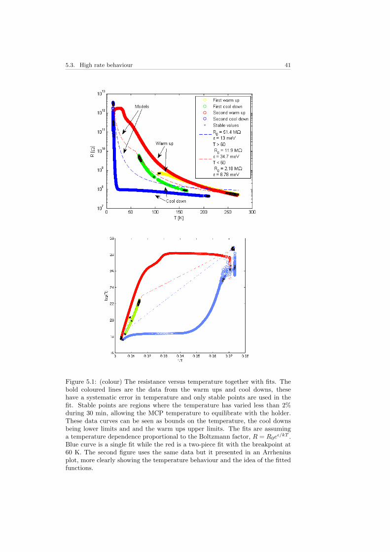
5.3. High rate behaviour 41

Figure 5.1: (colour) The resistance versus temperature together with fits. Thebold coloured lines are the data from the warm ups and cool downs, thesehave a systematic error in temperature and only stable points are used in thefit. Stable points are regions where the temperature has varied less than 2%during 30 min, allowing the MCP temperature to equilibrate with the holder.These data curves can be seen as bounds on the temperature, the cool downsbeing lower limits and and the warm ups upper limits. The fits are assuminga temperature dependence proportional to the Boltzmann factor, R = R0e

ε/kT .Blue curve is a single fit while the red is a two-piece fit with the breakpoint at60 K. The second figure uses the same data but it presented in an Arrheniusplot, more clearly showing the temperature behaviour and the idea of the fittedfunctions.


1100 1200 1300 1400 1500 1600 1700 1800 1900 2000 210010

4

105

106

107

108

MCPKbiasKvoltageK[V]

Gai

nK[e− ou

t/e− in

]

14KKKfit

70KKKfit

100KKKfit

150KKKfit

300KKKfit

14KKKvalues

70KKKvalues

100KKKvalues

150KKKvalues

300KKKvalues

Figure 5.2: (colour) The gain bias dependence together with curves fitted tolow bias values, 1200-1500 V. Error bars show the propagated error from theinstrument accuracy.

0 100 200 3000

2

4

6

8

10

12

14

16

n [1

]

T [K]0 100 200 300

0.02

0.021

0.022

0.023

0.024

0.025

0.026

0.027

0.028

0.029

0.03

κ[V−

1 ]

T [K]

Figure 5.3: (colour) The temperature dependence of the fitted gain parametersfor low gain, 1200-1600 V. The error bars show the 95% confidence interval.n is the average number of cascades in a channel and should essentially beingconstant with temperature and any temperature dependence should be seen inκ which when multiplied by the energy of incoming electrons gives the numberof released electrons from the channel wall.

5.4. Pulse behaviour 43

105

106

107

108

109

10−3

10−2

10−1

100

101

Electrons.in

Inte

nsity

/Ele

ctro

ns.in

.=.A

*Gai

n.+

.B.[a

.u]

Figure 5.4: (colour) The decrease in gain as the total amount of input chargeincreases. Error bars come from instrument accuracy.

5.3.1 Gain saturation at room temperature

With the optical setup it was possible to measure saturation with pulses, as canbe seen in Figure 5.4 where the gain shows a clear drop with increased pulsewidth (plotted as number of electrons). The time constant is in the order of 10ms in these measurements. Done at 100 Hz pulses, 400 ms exposure, calibratedby measuring 0.3 nA when using 10 µs pulses, the pulse width was varied andthe total amount of charge was assumed to be proportional to the pulse width.

5.3.2 Constant current saturation

In the optical test when the MCP was run with a constant input, an unexplainedeffect appeared as the input became stronger. The signal image, which at firstappeared as a disc in the centre as expected, started to spread out and eventuallyalso became darker in its centre. At the highest rates measured, the signal imagedisappeared completely and the entire phosphor was glowing instead, see Figure5.5. The possible reasons for this behaviour are discussed in the next section.

5.4 Pulse behaviour

The initial pulse tests, using a Faraday cup, did not give any clear informationregarding the behaviour of the MCP with a pulsed input signal. The main cause


Figure 5.5: 12 images showing how the phosphor started glowing and the centrebecame darker as the number of input electrons increased. This is in contrast tothe expected dot with increasing intensity which can be seen in the beginning.

for this was the crosstalk between the waveform generator and the Faraday cup,making it too hard to distinguish signal from crosstalk. The intention of the testsin the optical setup was to avoid the crosstalk and create a test setup resemblingthe final detector. However, the unexplained constant current saturation effectsseen previously also seemed to be apparent when pulsing, see Figure 5.6, givingvery weak and spread out signals. The origin of this effect is unknown but threemain ideas have been discussed.

• Due to changing potentials and/or electron-electron repulsion the electronsspread out and create the ring shape when the intensity increases. Thetest was however done two times. The first time by varying the screenpotential, which of course could change the ion-optical properties of thesystem. The second time the potentials were fixed and only the filamentcurrent was changed and the result was still the same. This suggests that itis not the potentials changing, or more precisely that any potential changesmust come from the currents themselves and any voltage drop they createdue to internal resistances. No internal resistances are however knownthat could create this effect.

• Secondary electrons and non-uniform replenishing of MCP channels. Ifsome of the electrons start impacting the surface of the MCP instead ofthe channels they can start knocking out secondary electrons which spreadout across the MCP and make more channels fire. This would explain theincreased glowing area. If the MCP then starts to saturate it will replenishthe channels closest to the rim first and the centre channels will receive

5.5. Time constant 45

Figure 5.6: One way of controlling the number of input electrons when pulsingis by regulating the length of the pulse. These 6 images, with pulse lengths0.1, 0.5, 1, 5, 10, 100 µs, show the phosphor screen for increasing pulse lengthsat constant frequency and filament current. The 10 µs pulse corresponds toroughly 108 electrons. The line in the images is a damage on the phosphor.Colour has been inverted to ease viewing.

less current, not replenish and become dark.

• Secondary electrons getting knocked out backwards from the phosphorwhich creates a glowing disc with the same principle as mentioned in theprevious case. Unfortunately, this does not explain the dark region incentre.

5.5 Time constant

From the simple timing tests when saturating the MCP we see a recuperationtime of approximately 4 s at 14 K. This is better than the estimated timeconstant of 4 TΩ · 100 pF = 400 s at these temperatures.

5.6 Phosphor screen

During the tests the phosphor screen was slightly damaged and it needed to bechecked to know if the data from it could still be used. To verify the behaviour


0 0.2 0.4 0.6 0.8 1 1.2 1.4

xI10−4

0

0.5

1

1.5

2

2.5

3

3.5

4

4.5

5xI10

6

PhosphorIcurrentI[A]

Tot

alIli

ghtIi

nten

sity

I[a.u

]

InputIcurrentIvsIoutputIlightIwithI1IsIshutterIandImasterIgainI50

I

yI=I3.4e+010*xI+I9.3e+004

Figure 5.7: (colour) The relative increase of the phosphor intensity to the currenton the the phosphor screen. The behaviour was linear, as seen by the fit, eventhough the phosphor had received some damage at this point. Error bars frominstrument accuracy.

of the phosphor screen we controlled that the total intensity of the phosphorscreen is linear to the current coming from the MCP.

As expected on an undamaged phosphor screen we still see in Figure 5.7 thatthe total intensity was linear to the number of electrons hitting the screen. Sincethe phosphor screen is harder to analyse with the damage it is still good to knowthat the total intensity and the phosphor screen current are relevant measuresof the output from the MCP.

Chapter 6

Discarded designs

This chapter discusses the different technologies and design options that wereconsidered during the course of the design but that for various reasons were dis-carded. The options are briefly explained together with their potential benefitsand the reason for their discarding.

6.1 Segmented Faraday Cup

A segmented Faraday cup (SFC) is an array of anodes, simple Faraday cups, thatcan be used to measure and image incoming charged particles/charge clouds.Each anode has its own read out line which enables precise measurements of thecharge as well as arrival times. With high enough anode density one can imagecharge clouds and their distributions using the accumulated charge on eachanode. SFCs are often used for characterisation of charged particle beams. Thebenefits of SFCs are the high resolutions in time and charge and the relativelysimple electronics making it easy to implement them at low temperatures.

The main drawbacks of the SFC is the low spatial resolution since each anodeis macroscopic and manufacturing SFCs with smaller anodes is difficult due tothe increase in readout channels. The latter also significantly complicates thereadout, increasing the cost of the required peripheral equipment. In the case ofan MCP detector the SFC also needs to be biased at high voltage (3 kV) whichcomplicates the readout even further but can be solved by using high voltagedecoupling capacitors. The design considered by AEGIS included an ASICthat was designed to read out high voltage decoupled signals in parallel insidethe cryostat. The data would have been serially transmitted to the outside.The main reasons for discarding this option was the mechanical difficulty inmanufacturing the SFC, finding suitable high voltage decoupling capacitors andoperating the ASIC in the cryostat without having a too high heat load in thecryostat.

Berggren, 2013. 47

48 Chapter 6. Discarded designs

Figure 6.1: (colour) A hexagonal delayline detector which also shows how theactual delay line is wired around theholder. Image: RoentDek Gmbh

6.2 Delay Line Detector

A delay line detector (DLD) uses two or more so called delay lines to measurethe position charge clouds. A delay line is a metal wire anode. When a chargeimpacts a point on the delay line it sends out two charge pulses in oppositedirections of the wire. By measuring the arrival time of these two pulses one cancalculate the impact position along the line by multiplying the time differencewith the signal speed in the wire. To create an imaging surface the wire is tightlywound around (but isolated from) an attracting anode so that the wire createsa layer of parallel lines. With one of these layers it is possible to determinethe position along one axis and for full xy positioning two or more layers ofthese wires around the anode are used. Delay lay line detectors in principlealways use MCPs as initial electron multipliers to get large enough signals ontothe wires. In addition, to improve performance, delay line detectors often useadditional techniques to improve performance such as double signal wires forincreased signal speed and three layer hexagonal design to increase resolution(see Figure 6.1. The delay line has high resolution in both time and charge aswell as spatially making it very precise for detecting and imaging particles.

The main drawbacks of the DLD are the limited count rate and the need forcharge spread. At high count rates, ambiguities are often seen when matchingcorresponding pulses which leads to completely losing the spatial informationof incoming hits. This can however be solved by using a phosphor screen asthe attracting anode so that high rates can be studied by imaging the phosphorscreen. It is important that the charge output from the MCP is spread out tomake sure that it hits parts of the wire in both layers. The latter is the mainreason for not using a delay line detector in the AEGIS experiment. We cananalyse the Lorentz force on an electron in an electric and magnetic field

F = q(E + v × B)

where E = Ez and B = Bz and with an initial velocity

v0 = vr r + vz z.

This gives rise to what is known as cyclotron motion so that the magnetic field

6.2. Delay Line Detector 49

Figure 6.2: (colour) In a magnetic field the spread of electrons is severely low-ered. The graph shows histograms of the distributions, the wider distribution(red) showing the spread without a magnetic field and a narrower (green) whichshows the distribution with a magnetic field. The distribution with a magneticfield essentially overlaps with the initial distribution (blue) at this scale.

will cause the particle to move in spirals with a radius of

rcycl =mevrqB

Estimating these values in the experiment we get rcycl ≈ 20 µm. Comparingthis to the radius of the spread in a delay line detector without a magneticfield, 2 mm, the spread is significantly reduced and thereby also the detectionability. This can also be seen in COMSOL simulations, see Figure 6.2, wherethe electrons radial spread when emitted from a channel is practically stopped.The phenomena and problem has also been confirmed by delay line manufacturerRoentDek Gmbh.

An additional complication with using a delay line detector was that it wouldhave been hard to fit it mechanically inside the experiment while still maintain-ing a large enough imaging area. It would probably have required a customdesign which would have considerably increased the cost.


6.3 Direct electron detection using a CCD

One potential option that was not tested is to directly detect incoming electronsusing a bare CCD chip connected to dedicated control electronics. A CCDordinarily uses photon to electron converting layer(1 electron per photon) togenerate electrons which are collected in the pixels of the chip. By acceleratingincoming electrons with a sufficient energy (in the order of 1 keV) it shouldbe possible to penetrate electrons deep enough into the CCD to be collectedby the pixels. The CCD can be operated as a regular CCD and the imageintensity would be interpreted as accumulated charge instead of light intensity.This would enable good spatial resolution and charge resolution since scientificgrade CCDs can have a sensitivity in the range of 100 electrons.

There are however some questions regarding the ability of a CCD to work inlow temperature and the possible shutter time and read out speed. It has beenshown that a CCD could be operated in 4 K environment by locally heatingit to about 70 K [12][13][14]. The shutter time, since a CCD usually operatesby charge integration, limits the time resolution of the read out system makingit hard to time single events and during read out there is no detection at all,imaging would then have to be made by integrating over the whole period ofinterest. The CCD would also have to be operated at high voltage, demandingsome sort of high voltage decoupling to the read out electronics. This optionwas not investigated further in benefit of more reliable and tested techniques.

6.3.1 Image conduit

An option for reading out a phosphor screen is to use an array of fused opticalfibers, a so called image conduit. This can be used to transfer a phosphor screenimage from the cryostat out to room temperature with low light loss comparedto direct imaging. One can also combine the image conduit with optical stagesto shrink the image and also coat the input of the image conduit so that itbecomes a phosphor screen and there is no light loss between the phosphorand the conduit. This option is however very expensive and not good enoughcompared to the much cheaper lens system chosen.

6.3.2 Camera in cryostat

Placing a phosphor readout camera inside the cryostat, instead of outside, to-gether with an optical system, would considerably improve the light yield andresolution of the phosphor image. Even though it has been shown that CCDscan operate at low temperatures a custom camera system is much too expensiveto develop and construct, an option is then commercially available products. Itis, however, much harder to operate these at low temperature since other com-ponents in the cameras are also sensitive to temperature and can stop workingbelow certain temperatures.

A test was done on a Logitech C270 web camera to see at how low temperaturesit could be run and how it behaved at various temperatures. The camera,

6.3. Direct electron detection using a CCD 51

stripped from its housing, was first placed in a vacuum chamber connected to aheat sink which was cooled using liquid nitrogen. The setup reached −30 C andthe only noticeable difference was slightly improved image quality in terms ofless noise. The camera was later removed from the vacuum and slowly loweredinto a liquid nitrogen canister while monitoring the image and temperature ofthe camera board. The camera showed improving image quality down to −80 Cwhere image artifacts started to appear such as coloured lines and loss of colourchannels. At −110 C the camera image was completely unreadable. The exactreason for the behaviour has not been determined but it is not believed to berelated to the actually CCD chip but instead comes from problems arising inthe image coding hardware or USB interface.

Chapter 7

Specification and design ofchosen system

After tests and research the candidate system with the best prospects was con-cluded to be the one with a MCP stack followed by a phosphor screen, an opticalfocusing system and a CCD-camera placed outside of the low temperature re-gion. The technical details of the system are also summarised and described inAppendix B.

7.1 Microchannel plates

The MCP is a good choice for detection of many kind of ionising particles withhigh position and time resolution. The MCPs tested, Hamamatsu F1217-01,is a good choice that fulfils the detector demands but with some restrictionsin operation. A chevron stack is necessary and sufficient for single particledetection. The weakest measurable signals during the tests were in the range of105 electrons which also is the lower span of the chevron stack gain range, givinga dynamic range of two orders of magnitude up to the maximum gain of 107.The tested MCP size of 50 mm diameter and with a 42 mm active area diameteris larger than necessary for the detector. The initial ionising rings will have adiameter of 20 mm and if the MCP is placed directly after these any additionalactive area is superfluous. The additional active area could however be used ifthe MCP was moved further back into a region where the magnetic field startsto diverge. The field could then be used as a magnifying lens and particlesspread out across a larger area of the MCP. A large benefit of placing the MCPas close as possible to the ionising rings and trap is that it could be possible todirectly detect unionised hydrogen. However, since the lifetime of the excitedstates is relatively unknown it is hard to determine whether it is necessary toplace it close to the traps or not under the prevailing field conditions; as a shortlifetime would mean that nothing would be detected. For hydrogen detection,both with and without ionising rings the MCP should be operated at full gain.For plasma imaging a low gain would be preferred, but if it is interesting to

Berggren, 2013. 53

54 Chapter 7. Specification and design of chosen system

measure single particles (for arrival times for example) the gain still needs to belarger than 105 (to create measureable signals).

7.2 Phosphor screen

The choice of a phosphor screen is convenient since it gives a natural high voltagedecoupling from the MCP. The P43 phosphor tested, Beam Imaging 40-008,was shown to be good enough to do both single particle detection and plasmaimaging (the later with possible restrictions). Due to the gamma (and eventualUV) flash shortly after the positronium combination and the long time constantof the MCP (making it to difficult to vary its potentials within a reasonabletime) the phosphor will be triggered at this moment. To avoid that the lightfrom gammas overlaps with the light produced by hydrogen and electrons it isimportant that the decay time of the phosphor is shorter than the time of flightof the hydrogen. This has been estimated to be in the range 10 µs to a few100 µs, which excludes the use of the standard P43 phosphor which has a decaytime of 1 ms but is in the range of fast standard phosphors such as P46 andP47 which have decay times of 300 ns and 55 ns respectively.

7.3 Lens system

The lens system consists of three lenses placed relative to each other as inthe optical test setup, see Chapter 4.4. This will give approximately 15 timesmore light than without lenses and also parallelises the light so that the cameraposition is less sensitive in its position along the optical axis. Due to the fieldof view of the camera it is still interesting to place it as close as possible to thelast lens while still keeping the entire lens inside the image.

7.4 Camera

Despite no explicit vacuum compatibility, the Thorlabs CCD camera was foundto work well in vacuum and fulfils the necessary demands. The electronic shut-ter time can be taken down to 1 ms to lower noise and the shutter can alsobe remotely triggered which is an important feature when synchronising thecamera with the hydrogen production and avoiding exposing the sensor at thegamma flash. Exact settings and operation need to be further investigated. It isimportant to note that during the optical tests it was not possible to operate thecamera using the 5 m cable with trigger wire but it did work with a 3 m cableand using a high power USB outlet (allowing up 1.5 A instead of the standard0.5 A on USB 2.0 port).

Chapter 8

Discussion

This chapter discusses the work covered and possible future work. It starts witha discussion on the performance and operation of the final detector. We thengo on discussing future work and optional designs.

8.1 H* detection

The main goal of the work described here has been to develop a design todetect single excited hydrogen atoms. An initial ionising stage of the detector,described in detail in [5] generates the charged particles that need to be detectedby means of an MCP.

Single particle detection is governed by the probability of producing a primarycharge in one of the MCP channels and the actual highest possible gain of theMCP at the necessary low operating temperatures of the experiment. From testsan acceptable decrease of 50% was found for the gain at temperatures down to14 K. It should be possible to reach a primary detection efficiency of up to 85%by choosing a proper accelerating voltage. This number is considered not to beaffected by a low operating temperature. With the proposed design it shouldhence be possible to detect single particles and to comply with the measurementrequirements for Rydberg hydrogen atoms generated and manipulated in thePenning traps in the AEGIS experiment.

Direct detection of Rydberg hydrogen should also be possible and for the statesthat cannot be ionised, n ≤ 18, some of them, n ≥ 14, will be able to be detecteddirectly by the MCP instead.

An initial burst of gamma radiation and UV light can possibly trigger channelson the MCP. The number of triggered channels should however be small com-pared to the total number of available channels (< 1%) and should not have alarge effect on the detection efficiency and the output signals of hydrogen events100 µs later. These events will however trigger the phosphor screen and it istherefore important that the decay time of the phosphor is shorter than thetime of flight of the hydrogen atoms.

Berggren, 2013. 55

56 Chapter 8. Discussion

Figure 8.1: (colour) The totalintensity with a saturation capas a function of radius for aspherical charge cloud.

8.2 Plasma cloud imaging

The plasma imaging is at the other end of the detection spectrum and consistsof a large signal for an extended time period on a limited area. This will almostunavoidably saturate the channels of the MCP but as long as the MCP has hadtime to recharge it should be possible to image the silhouette of the cloud. Theintensity will most likely saturate in the center of the image but the part ofthe edge of the cloud image, which has much fewer events, should still have anintensity proportional to the number of events (see Figure 8.1).

8.3 Electron Time-Of-Flight

To measure the time of flight of the initial electrons in the plasma cloud oneneeds to make certain that the gain of the MCP is high enough for single particledetection, this means at least a gain of 105 but preferably around 106. Theoutput, the phosphor screen, will then also have to be treated as a Faraday cupwith a fast signal readout so that the arrival of the signal can be measured withhigh precision. For this, one also needs to make certain that the noise is ata minimum so that it is possible to distinguish the initial electrons from darkcounts.

8.4 Lowering γ noise

In case a reduction of the gamma events would be required there are certainmeasures one could take to lower their influence. The main two are addingshielding and moving the MCP away from the trap. Shielding could be done byadding material between the MCP and trap with a high absorption coefficient.This requires a lot of material and can be hard to implement in a good wayaround the trap without interfering with other systems. The other option is toposition the MCP further away from the trap, while still keeping the ionisingrings close to it. By doing this, reducing the solid angle to the trap, one would

8.5. Characterising detector and dark counts 57

then make use of the magnetic field lines to detect the charged particles that areionised in the first stage. However, when moving back the MCP it is less likelythat it will detect unionised hydrogen and there is also the question regardinghow far it is possible to move the MCP while still remaining in the homogeneouspart of the magnetic field.

8.5 Characterising detector and dark counts

After the construction and installation of the final detector it is important tocharacterise the noise and performance of the detector in its actual operatingenvironment. Important steps are determining expected signals and noise tomore easily sort between noise and actual events. Properties of interest is thengain, recharge time and pulse shape for actual signals as well as spectrum andpulse shape of dark counts. Understanding the spectrum of the dark counts itwill ease the process of filtering out noise from the actual measurements and alsogive some better knowledge about the noise over signal ratio for the differentmeasurements.

8.6 Other MCP properties

There are other properties of MCPs and especially MCP stacks that have notbeen studied in this thesis, especially the impact of a spacing between the MCPs,independent biasing of the MCPs in the stack and local differences in gain andbehaviour across the MCP surface.

It is known that using a spacing has a strong effect on the behaviour of MCPstacks since it allows electrons to spread out over more channels in the latterstages. This can increase the total gain of the stack but it also gives a lowerresolution, even though the resolution of the MCP is not commonly the limitingfactor. However, in the light of the experiment, the effects of a spacing is lessinteresting since the strong magnetic field will reduce the spread of the electrons.This will in principle remove any beneficial effects one would get from a spacing.

Using an electrode as the spacing allows independent regulation of the supplyvoltages for the stages of the MCP stack. This is useful when there are differ-ences in the resistance between the MCPs used in the stack. If the resistancediffers between the MCPs there will be differences in the individual supply volt-age for each MCP. This will give different gains in the stages and it is possiblethat the individual voltages are higher than the recommended maximum supplyvoltage which can shorten the lifetime of that MCP.

There can also be differences in gain and recharge time locally across the MCPdue to imperfections from the manufacturing, damage or dirt particles. Onecould for example also imagine a radial dependence in gain for example due tothe surface resistance of the MCPs, which should give a slight voltage drop inthe centre compared to points closer to the edge. This effect should however benegligible since the surfaces are usually designed to have a resistance of 200 Ω

58 Chapter 8. Discussion

from one side of a surface to the other and this is much lower than the 40 MΩthrough the MCP.

8.7 Direct electron detection with CCD

The option of using a bare CCD, or an array of them, to directly detect elec-trons was an option that would have been interesting to investigate further.Although the cryogenic conditions of the experiment was a complication forthis technology the principle might be interesting to use in other applications,if it works.

8.8 Next steps

The next part of the development should be the mechanical design and con-struction of the detector. This should be done while keeping the operationaspects in mind so that it is possible to read out the wanted signals, trying toavoid crosstalk between components, reduce risk of sparking etc and minimisingnoise. After the design, read out software needs to be made that can synchro-nise with other parts of the experiment, such as the trap controls. To be ableto perform all the wanted measurements the camera needs to be synchronisedand timed with a lag to avoid any initial flash. This should also be synced withthe electronic readouts on (preferably) all electrical connections (rings, MCPsand phosphor).

Appendix A

Explanation of additionalconcepts

This appendix describes different technologies and principles mentioned in thethesis but that are not directly relevant to the work.

A.1 The Weak Equivalence Principle

The weak equivalence principle states that point particles with same initial posi-tions and velocities will follow the same trajectories regardless of their mass andcomposition. It is the everyday interpretation of gravity as a force, proportionalto the mass, and that a gravitational acceleration replaced with a correspondingacceleration will give rise to the same motion. The classical example of this isthe astronaut in a closed spaceship. Accelerating with 1g in space he will not beable to distinguish it from being at rest on the surface of the earth, see FigureA.1.

A.2 Penning traps

The Penning trap is an electromagnetic trap used to trap charged particles. Bycombining an electric and magnetic field it is possible to confine a particle to alimited volume and the size of the volume depends the strength of the fields aswell as of the temperature of the particles.

There are different ways of creating the necessary electric potentials. TheAEGIS experiment will use an open end cylindrical trap construction whichalso allows particles to be inserted and ejected from the trap via the ends.The simplest form uses three electrodes to create a well potential that focusescharged particles in the centre. For electrons the potentials would be biasedwith low potentials on edge electrodes and a high potential on centre potential,

Berggren, 2013. 59

60 Appendix A. Explanation of additional concepts

a = g

gg

Earth

Figure A.1: According to the weak equivalence principle, an astronaut in aclosed spaceship will not be able to distinguish between being at rest on earthand accelerating at 1g.

A.3. Rydberg atoms 61

Figure A.2: (colour) The potentials, φ(z), and electrical field strength, E(z),inside a cylindrical Penning trap at a fixed radius. In combination with a strongmagnetic field along the z-axis the potentials will trap the corresponding chargein the central potential well.

see Figure A.2. This will cause the electrons to be attracted to the centre elec-trode, to prevent them from going in to centre electrode one applies a magneticfield along the cylindrical axis. The magnetic field will align the particles withthe axis and by the cyclotron effect confine them radially.

To extract electrons, the potentials needs to be changed in a controlled manner.By raising the potential of the ring at which one wants to eject the particlesand lowering the potential of the centre electrode the electrons will start tomove towards that edge electrode. Since the electrons are still aligned by themagnetic field this is a good process for controlling charged particles.

A.3 Rydberg atoms

Rydberg atoms are highly excited hydrogen atoms with a main quantum num-ber, n, above 15. These atoms are approximately well described by the Bohrmodel and at these high quantum numbers the electrons become very weaklybound and the their orbital radius extremely large. This gives Rydberg atomsinteresting properties such as enhanced susceptibility to electric and magneticfields as well as increased increased geometrical cross-section. The latter is ofinterest in particle physics since it also enhances the cross section of interactionwith other particles. The increased susceptibility of electric and magnetic fieldsalso makes processes such as Stark acceleration and field ionisation easier.

A.4 Stark acceleration

Stark acceleration is the method of using inhomogeneous electric fields to accel-erate particles consisting of charged particles but with a zero net charge.

62 Appendix A. Explanation of additional concepts

Modelling a Rydberg hydrogen atom as an electric dipole. Say that the vectorfrom the electron, charge −q, to the proton, charge +q, is d. The centre of thedipole is located at x. This gives rise to a force on the dipole that is

F = q(E(x + d/2)−E(x− d/2)).

As expected we see that for homogeneous fields and small d the force is closeto zero. This is however close to a differential so let us investigate a componentof F and do a Taylor expansion

Fx = q(Ex(x + d/2)− Ex(x− d/2)) ≈ q∇Ex(x) • d

If we now also use the fact that E = −∇φ we get

Fx = −q((δ2φ

δx2,δ2φ

δxδy,δ2φ

δxδz) • d)

Doing this for all components we see that we actually get the Hessian of φ in x,

F = −qH(φ)|xd = −H(φ)|xp.

Where we have used the dipole vector p = qd. From this we see that by havingan inhomogeneous electric field it is possible to exert forces on dipoles and bythat accelerating for example hydrogen or antihydrogen.

Appendix B

Baseline design

This appendix summarises the work on the hydrogen detector and is meant tobe an easily accessible reference for the continued development, especially forthe mechanical design which should be the next step.

B.1 Ionising rings

Based on the work by Olof Ahlen [5] it was decided that the best design for theionising rings would be three rings with with the dimensions specified in FigureB.1. The voltage used on the positive anodes should be the extreme allowed,5000 V, to increase the detection efficiency as much as possible.

For hydrogen detection it is also recommended that the rings are operated in anelectron trapping mode for hydrogen detection. For this the electrodes shouldbe biased low, high, low (recommended 0 V, 5000 V, 0 V). The reason fortrapping is to avoid noise from positronium decay and UV light when detectingthe hydrogen on the MCP.

The thickness of the rings is not an essential factor but the rounding of thecorner is. The corners are were the strongest electric fields will be and werethere is a risk of sparking. It is therefore important to round the corners toreduce the risk of sparking but the rounding must be small enough not to affectthe field inside the rings too much. The calculations done with the settingsabove used a 1 mm thick ring which had rounded corners with a 0.5 mm radius.

B.2 MCP

The tested MCPs F1217-01 should be sufficient for the detector and to reducecosts one could use the ones available in the experiment. If new MCPs arebought it is not necessary with the large diameter of the F1217-01 (50 mm) andone should buy MCPs with diameters in the range 20-30 mm instead, this willdecrease the time constant of the MCP in the system as well as the cost.

Berggren, 2013. 63

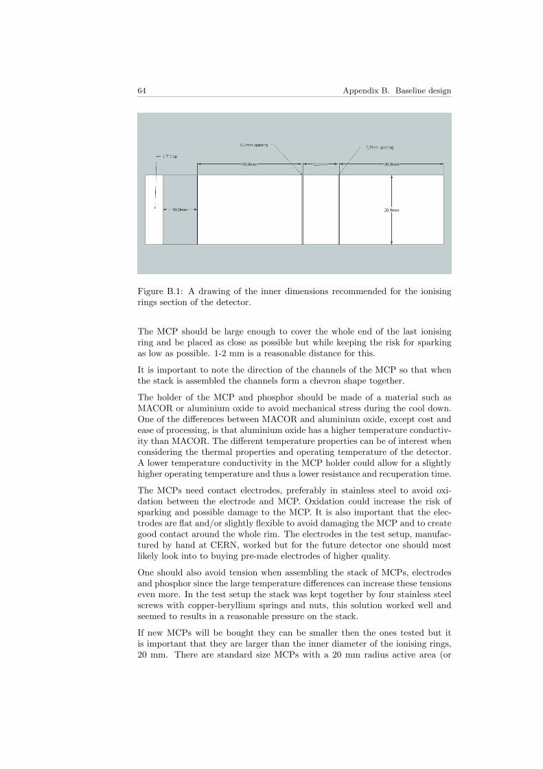
64 Appendix B. Baseline design

Figure B.1: A drawing of the inner dimensions recommended for the ionisingrings section of the detector.

The MCP should be large enough to cover the whole end of the last ionisingring and be placed as close as possible but while keeping the risk for sparkingas low as possible. 1-2 mm is a reasonable distance for this.

It is important to note the direction of the channels of the MCP so that whenthe stack is assembled the channels form a chevron shape together.

The holder of the MCP and phosphor should be made of a material such asMACOR or aluminium oxide to avoid mechanical stress during the cool down.One of the differences between MACOR and aluminium oxide, except cost andease of processing, is that aluminium oxide has a higher temperature conductiv-ity than MACOR. The different temperature properties can be of interest whenconsidering the thermal properties and operating temperature of the detector.A lower temperature conductivity in the MCP holder could allow for a slightlyhigher operating temperature and thus a lower resistance and recuperation time.

The MCPs need contact electrodes, preferably in stainless steel to avoid oxi-dation between the electrode and MCP. Oxidation could increase the risk ofsparking and possible damage to the MCP. It is also important that the elec-trodes are flat and/or slightly flexible to avoid damaging the MCP and to creategood contact around the whole rim. The electrodes in the test setup, manufac-tured by hand at CERN, worked but for the future detector one should mostlikely look into to buying pre-made electrodes of higher quality.

One should also avoid tension when assembling the stack of MCPs, electrodesand phosphor since the large temperature differences can increase these tensionseven more. In the test setup the stack was kept together by four stainless steelscrews with copper-beryllium springs and nuts, this solution worked well andseemed to results in a reasonable pressure on the stack.

If new MCPs will be bought they can be smaller then the ones tested but itis important that they are larger than the inner diameter of the ionising rings,20 mm. There are standard size MCPs with a 20 mm radius active area (or

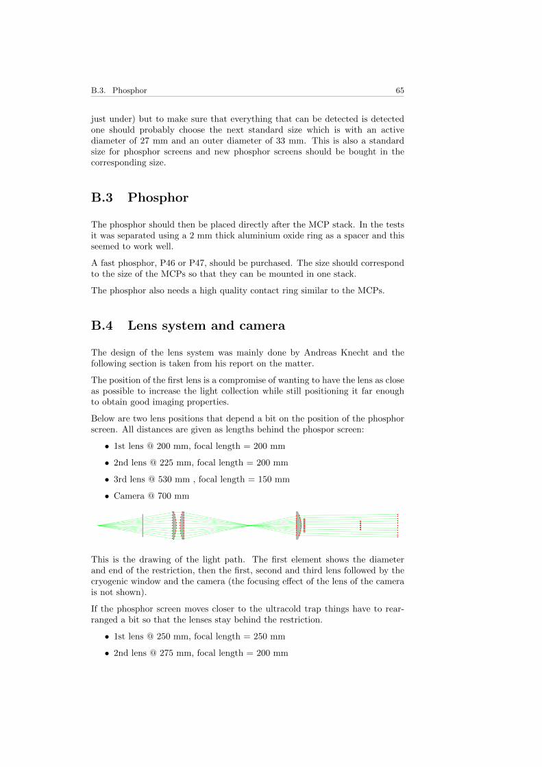
B.3. Phosphor 65

just under) but to make sure that everything that can be detected is detectedone should probably choose the next standard size which is with an activediameter of 27 mm and an outer diameter of 33 mm. This is also a standardsize for phosphor screens and new phosphor screens should be bought in thecorresponding size.

B.3 Phosphor

The phosphor should then be placed directly after the MCP stack. In the testsit was separated using a 2 mm thick aluminium oxide ring as a spacer and thisseemed to work well.

A fast phosphor, P46 or P47, should be purchased. The size should correspondto the size of the MCPs so that they can be mounted in one stack.

The phosphor also needs a high quality contact ring similar to the MCPs.

B.4 Lens system and camera

The design of the lens system was mainly done by Andreas Knecht and thefollowing section is taken from his report on the matter.

The position of the first lens is a compromise of wanting to have the lens as closeas possible to increase the light collection while still positioning it far enoughto obtain good imaging properties.

Below are two lens positions that depend a bit on the position of the phosphorscreen. All distances are given as lengths behind the phospor screen:

• 1st lens @ 200 mm, focal length = 200 mm

• 2nd lens @ 225 mm, focal length = 200 mm

• 3rd lens @ 530 mm , focal length = 150 mm

• Camera @ 700 mm

This is the drawing of the light path. The first element shows the diameterand end of the restriction, then the first, second and third lens followed by thecryogenic window and the camera (the focusing effect of the lens of the camerais not shown).

If the phosphor screen moves closer to the ultracold trap things have to rear-ranged a bit so that the lenses stay behind the restriction.

• 1st lens @ 250 mm, focal length = 250 mm

• 2nd lens @ 275 mm, focal length = 200 mm


• 3rd lens @ 580 mm , focal length = 150 mm

• Camera @ 750 mm

Here the first two lines show the beginning and end of the restriction. Theposition of the last lens is not very critical and gives similar results in a range560 – 600 mm.

Using LEDs and comparing the cases with and without the lenses gives enhance-ment factors of about x15 for the first setup. Positioning the first lens at 250mm instead of 200 mm then leads to a reduction of photon collection of about35% which is acceptable.

B.4.1 Layout in AEGIS Apparatus

The three lenses will be mounted inside the anticryostat within the larger vol-ume on the downstream side. This area will be closed by a vacuum windowcompatible with cryogenic temperatures. The camera is then placed in theOVC behind the liquid nitrogen shield at approximately room temperature. Inorder to reduce the thermal load onto the 4K region by the opening in the lNshield a glass disc can be pressed against the copper of the lN shield which istransparent for the visible light of the phosphor screen but blocks the infraredradiation (e. g. from http://www.uqgoptics.com/). The camera and the lensesshould be fairly well aligned. They should probably both be mounted onto thesame flange, i. e., the flange closing off the anticryostat.

B.4.2 Open issues and remarks

• Cables for MCP and electrodes need to be bought/organized for UHV andOVC

• Feedthroughs for UHV and OVC need to be bought/organized for MCPand electrodes. Feedthrough in OVC needs to be bought/organized forcamera (5 pins for USB communcation, 2 pins for hardware trigger). Inaddition feedthroughs as needed for heating and temperature sensing

• Cryogenic window and glass disc need to be bought/organized

• Mechanical design

• Once installed the focus of the lens of the camera has to be adjusted tothe right setting. It is insensitive to changes of the lenses within +/- 5mm so thermal shrinkage should be no problem.

• The camera switches on a status LED once powered. This should becovered inside the OVC in order to not interfere with the FACT detector.

B.4. Lens system and camera 67

• There are first LabView programs that interface with the camera available.They are saved on the desktop of the “aegisenv” account. “HydrogenCam-eraController Simple” is a good start. They are written in LabView 2011and need the Vision toolbox and the camera drivers installed.

• The USB cable of the camera cannot be too long. When we used the fulllength of the USB/Trigger cable of the camera (3 m) and extended theUSB cable on the outside the camera did not work. A total length ofabout 3 m thus seems to be about the maximum. One could probably userepeaters to increase that length.

Bibliography

[1] CERN, “About CERN.” http://home.web.cern.ch/about, 2013. [Online;accessed 2-July-2013].

[2] W. Bartmann, P. Belochitskii, H. Breuker, F. Butin, C. Carli, T. Eriksson,R. Kersevan, S. Maury, S. Pasinelli, G. Tranquille, et al., “Progress inELENA design,”

[3] D. K. et al., “AEgIS Experiment Commissioning at CERN.” 2012.

[4] M. Doser et al., “Exploring the WEP with a pulsed cold beam of antihy-drogen,” Class.Quant.Grav., vol. 29, p. 184009, 2012.

[5] O. Ahlen, “Rydberg Hydrogen Detector with n-state dependent Field Ion-ization,” master’s thesis, Chalmers University of Technology.

[6] J. L. Wiza, “Microchannel plate detectors,” Nucl. Instrum. Methods,vol. 162, no. 1-3, pp. 587–601, 1979.

[7] G. Fraser, M. Pain, J. Lees, and J. Pearson, “The operation of microchannelplates at high count rates,” Nuclear Instruments and Methods in PhysicsResearch Section A: Accelerators, Spectrometers, Detectors and AssociatedEquipment, vol. 306, no. 1, pp. 247–260, 1991.

[8] Hamamatsu Photonics K.K., MCP Assembly, tmcp9002e01 ed.

[9] P. Roth and G. Fraser, “Microchannel plate resistance at cryogenic temper-atures,” Nuclear Instruments and Methods in Physics Research Section A:Accelerators, Spectrometers, Detectors and Associated Equipment, vol. 439,no. 1, pp. 134–137, 2000.

[10] J. Schecker, M. Schauer, K. Holzscheiter, and M. Holzscheiter, “The per-formance of a microchannel plate at cryogenic temperatures and in highmagnetic fields, and the detection efficiency for low energy positive hydro-gen ions,” Nuclear Instruments and Methods in Physics Research Section A:Accelerators, Spectrometers, Detectors and Associated Equipment, vol. 320,no. 3, pp. 556–561, 1992.

[11] J. H. Hubbell and S. M. Seltzer, “Tables of X-ray mass attenuation coeffi-cients and mass energy-absorption coefficients 1 keV to 20 MeV for elementsZ= 1 to 92 and 48 additional substances of dosimetric interest,” tech. rep.,National Inst. of Standards and Technology-PL, Gaithersburg, MD (UnitedStates). Ionizing Radiation Div., 1995.

Berggren, 2013. 69

70 Bibliography

[12] P. G. Lucas, R. G. Matley, M. S. Thurlow, and W. Y. Wong, “Improvedoptical system for visualising convection in liquid helium,” Physica B: Con-densed Matter, vol. 284-288, Part 2, no. 0, pp. 2061 – 2062, 2000.

[13] R. Wagner, P. Ras, P. Remeijer, S. Steel, and G. Frossati, “Observation of3He crystallization down to 1 mK using a cooled CCD camera,” Journalof Low Temperature Physics, vol. 95, pp. 715–728, 1994.

[14] H. Alles, J. P. Ruutu, A. V. Babkin, P. J. Hakonen, A. J. Manninen, andJ. P. Pekola, “Cooled video camera for optical investigations below 1 mK,”Review of Scientific Instruments, vol. 65, no. 5, pp. 1784–1785, 1994.

Copyright

The publishers will keep this document online on the Internet - or its possiblereplacement - for a period of 25 years from the date of publication barring ex-ceptional circumstances. The online availability of the document implies a per-manent permission for anyone to read, to download, to print out single copiesfor your own use and to use it unchanged for any non-commercial research andeducational purpose. Subsequent transfers of copyright cannot revoke this per-mission. All other uses of the document are conditional on the consent of thecopyright owner. The publisher has taken technical and administrative mea-sures to assure authenticity, security and accessibility. According to intellectualproperty law the author has the right to be mentioned when his/her work isaccessed as described above and to be protected against infringement. For ad-ditional information about the Linkoping University Electronic Press and itsprocedures for publication and for assurance of document integrity, please referto its WWW home page: http://www.ep.liu.se/

Upphovsratt

Detta dokument holls tillgangligt pa Internet - eller dess framtida ersttare -under 25 ar fran publiceringsdatum under forutsattning att inga extraordi-nara omstandigheter uppstar. Tillgang till dokumentet innebar tillstand forvar och en att lasa, ladda ner, skriva ut enstaka kopior for enskilt bruk ochatt anvanda det oforandrat for ickekommersiell forskning och for undervisning.overforing av upphovsratten vid en senare tidpunkt kan inte upphava dettatillstand. All annan anvandning av dokumentet kraver upphovsmannens med-givande. For att garantera aktheten, sakerheten och tillgangligheten finns detlosningar av teknisk och administrativ art. Upphovsmannens ideella ratt in-nefattar ratt att bli namnd som upphovsman i den omfattning som god sedkraver vid anvandning av dokumentet paovan beskrivna satt samt skydd motatt dokumentet andras eller presenteras i sadan form eller i sadant sammanhangsom ar krankande for upphovsmannens litterara eller konstnarliga anseende elleregenart. For ytterligare information om Linkoping University Electronic Pressse forlagets hemsida http://www.ep.liu.se/

c© 2013, Karl Berggren

Berggren, 2013. 71

department of physics, chemistry and biology - diva …647148/fulltext01.pdf · department of...

Documents