Department of Physics and Astronomy

University of Heidelberg

Bachelor Thesis in Physicssubmitted by

Lukas Layer

born in Schwabisch Hall (Germany)

2015

Development of a fast simulation tool for vertexing

studies in ALICE

This Bachelor Thesis has been carried out by Lukas Layer at thePhysikalisches Institut at the University of Heidelberg

under the supervision ofDr. Silvia Masciocchi

Abstract

The measurement of open heavy flavour hadrons plays a key role in the physicsprogram of the ALICE experiment. For the heavy flavour analysis it is crucial todetermine primary and secondary vertices with high precision. For this a new versionof the KFParticle vertexing package, that provides powerful tools for these challenges,is tested. In order to verify the algorithmic implementation of the code, a Unit Testhas been developed. To have full control over the input of the test, a fast simulationtool is implemented. Different observables of the decay D0 → π+K− and their chargeconjugates are studied. The results are compared to other vertexing packages. Toverify the fast simulation the same tests were repeated on full simulation and theresults compared. The recalculation of the primary vertex with different functionalitiesis investigated.

Zusammenfassung

Die Messung von Hadronen, die Charm und Beauty Quarks enthalten, spielt einewichtige Rolle im Programm des ALICE Experiments. Fur die Analyse dieser Mes-sungen ist es entscheidend primare und sekundare Vertizes mit hoher Prazission zumessen. Hierfur wird eine neue Version des KFParticle Vertexing Paketes getestet,das machtige Funktionen fur diese Aufgaben bereitstellt. Um die Implementation desAlgorithmus zu verifizieren, wurde ein Unit Test entwickelt und eine Fast Simulationimplementiert, die es ermoglicht Kontrolle uber den Input zu erhalten. VerschiedeneObservable des Zerfalls D0 → π+K− werden untersucht und mit anderen VertexingPaketen verglichen. Um die Fast Simulation zu verifizieren werden die selben Testsin einer vollen Simulation durchgefuhrt und die Resultate verglichen. Die Berechnungdes primaren Vertex wird mit verschiedenen Funktionen untersucht.

Contents

1 The Quark Gluon Plasma 9

2 The ALICE Experiment 112.1 The Detector . . . . . . . . . . . . . . . . . . . . . . . . . . . . . . . . . . . 112.2 The Inner Tracking System . . . . . . . . . . . . . . . . . . . . . . . . . . . 122.3 The Time Projection Chamber . . . . . . . . . . . . . . . . . . . . . . . . . . 122.4 Event reconstruction . . . . . . . . . . . . . . . . . . . . . . . . . . . . . . . 13

3 Open Heavy Flavour Hadrons 153.1 Overview . . . . . . . . . . . . . . . . . . . . . . . . . . . . . . . . . . . . . . 153.2 Measurement techniques in ALICE . . . . . . . . . . . . . . . . . . . . . . . 163.3 Recent results . . . . . . . . . . . . . . . . . . . . . . . . . . . . . . . . . . . 17

4 The KFParticle Vertexing Package 204.1 The Kalman Filter algorithm . . . . . . . . . . . . . . . . . . . . . . . . . . 204.2 Reconstruction of the primary vertex . . . . . . . . . . . . . . . . . . . . . . 204.3 Reconstruction of decayed particles . . . . . . . . . . . . . . . . . . . . . . . 204.4 Constrained fits . . . . . . . . . . . . . . . . . . . . . . . . . . . . . . . . . . 22

4.4.1 The topological constraint . . . . . . . . . . . . . . . . . . . . . . . . 224.4.2 The mass constraint . . . . . . . . . . . . . . . . . . . . . . . . . . . 22

4.5 Versions of KFParticle and motivation for a test . . . . . . . . . . . . . . . . 22

5 The ALICE Track Model 245.1 Equation of motion . . . . . . . . . . . . . . . . . . . . . . . . . . . . . . . . 245.2 Track parameters in ALICE . . . . . . . . . . . . . . . . . . . . . . . . . . . 24

5.2.1 Description of the parametrization . . . . . . . . . . . . . . . . . . . 245.2.2 Connection between parameters and measurement . . . . . . . . . . . 265.2.3 Implementation of the parametrization . . . . . . . . . . . . . . . . . 29

5.3 Covariance matrix of the track parameters in ALICE . . . . . . . . . . . . . 305.3.1 The covariance matrix . . . . . . . . . . . . . . . . . . . . . . . . . . 305.3.2 Track error caused by the detector . . . . . . . . . . . . . . . . . . . 315.3.3 Track error caused by multiple scattering . . . . . . . . . . . . . . . . 325.3.4 Track error caused by energy loss . . . . . . . . . . . . . . . . . . . . 325.3.5 Covariance matrix of the ALICE track parameters . . . . . . . . . . . 33

6 The Unit Test 356.1 The importance of Unit Tests . . . . . . . . . . . . . . . . . . . . . . . . . . 356.2 Design . . . . . . . . . . . . . . . . . . . . . . . . . . . . . . . . . . . . . . . 356.3 Generation of the particles . . . . . . . . . . . . . . . . . . . . . . . . . . . . 366.4 Extraction of the parametrization . . . . . . . . . . . . . . . . . . . . . . . . 36

6.4.1 Diagonal elements . . . . . . . . . . . . . . . . . . . . . . . . . . . . . 376.4.2 Off-diagonal elements . . . . . . . . . . . . . . . . . . . . . . . . . . . 39

6.5 Smearing of the parameters . . . . . . . . . . . . . . . . . . . . . . . . . . . 416.6 Example of the generation of a smeared particle track . . . . . . . . . . . . . 416.7 Definition of the test cases . . . . . . . . . . . . . . . . . . . . . . . . . . . . 44

7

7 Test Results of AliKFParticle 467.1 Quality of the daughters . . . . . . . . . . . . . . . . . . . . . . . . . . . . . 467.2 Reconstruction of the D0 . . . . . . . . . . . . . . . . . . . . . . . . . . . . . 47

7.2.1 Secondary vertex . . . . . . . . . . . . . . . . . . . . . . . . . . . . . 477.2.2 χ2/ndf and probability . . . . . . . . . . . . . . . . . . . . . . . . . . 507.2.3 Transverse momentum . . . . . . . . . . . . . . . . . . . . . . . . . . 517.2.4 Invariant mass . . . . . . . . . . . . . . . . . . . . . . . . . . . . . . . 53

8 Test Results of KFParticle 56

9 Primary Vertex and Impact Parameter with AliKFParticle 599.1 Primary ESD vertex . . . . . . . . . . . . . . . . . . . . . . . . . . . . . . . 599.2 Improvement of the resolution . . . . . . . . . . . . . . . . . . . . . . . . . . 609.3 The topological constraint . . . . . . . . . . . . . . . . . . . . . . . . . . . . 619.4 Impact parameter . . . . . . . . . . . . . . . . . . . . . . . . . . . . . . . . . 61

10 Conclusion and Outlook 6310.1 Test of AliKF . . . . . . . . . . . . . . . . . . . . . . . . . . . . . . . . . . . 6310.2 Test of KF . . . . . . . . . . . . . . . . . . . . . . . . . . . . . . . . . . . . . 6310.3 Further checks on the vertexer . . . . . . . . . . . . . . . . . . . . . . . . . . 6310.4 The Unit Test . . . . . . . . . . . . . . . . . . . . . . . . . . . . . . . . . . . 6310.5 Planned physics analysis with KF . . . . . . . . . . . . . . . . . . . . . . . . 64

8

1 The Quark Gluon Plasma

Figure 1: Phase diagramm of QCD [1]

Quantum ChromoDynamics (QCD) is the theory describing the strong interaction betweenquarks [2] which are the building blocks of matter and gluons which are the carriers of thestrong force. One of the crucial tests of QCD is the quantification of the behaviour of stronglyinteracting matter in the high temperature and high density limit. Under these conditions,QCD predicts the existence of a deconfined medium that is called the Quark Gluon Plasma(QGP). Deconfinement means that the colourless hadrons turn into a plasma consisting ofasymptotically free coloured quarks and gluons. Since observations have shown that no freequarks exist at the temperature and densities that we live in, a phase transition has to occur.The phase diagram of QCD is shown in figure 1.The mass of bound states of hadrons is not only determined by valence quarks, but alsoby virtual seaquarks and gluons. This leads to the fact that the constituent quark massMu,d ∼ 300MeV of up and down quarks is significantly higher than the calculated bare massmq that is in the order of a few MeV. Since the QCD Lagrangian contains a symmetry, calledchiral symmetry, for zero bare quark mass, the constituent quark mass Mu,d > 0 implies abreaking of this symmetry. The chiral symmetry of the QCD Lagrangian is predicted to berestored again, because the constituent quark mass becomes zero.The transition from the hadronic to the deconfined state is supposed to occur at a criticaltemperature TC [3]. Using a naive calculation for an ideal gas of massless pions and an idealquark gluon plasma with two flavours and three colours, the critical temperature can beapproximated by assuming that the gases are following the Stefan-Boltzmann law: P ∼ T 4

(fig. 2). Since thermodynamics predicts that a system always chooses the state of lowestfree energy and thus highest pressure, a rough estimate of TC can be found by a simpleextrapolation as TC ≈ 150MeV. The same simple estimation can be made for the energydensity: in this model the phase transition is of first order and thus an increase of theenergy density due to latent heat of the deconfinement is obtained. To get more preciseresults advanced theoretical concepts have been developed. Since the standard way of solvingQCD problems with perturbative calculations (pQCD) is not applicable in this region, alarge number of theoretical approaches [4] have been developed. To calculate the criticaltemperature, lattice QCD is used. The critical temperature is depending on the baryo-

9

Figure 2: The left panel shows a simple extrapolation of the critical temperature TC using an ideal gas ofpions and quarks. B is the bag pressure, which takes into account differences between the vacuumand ground state for partons in the QGP. The right panel shows the energy density in the twophase ideal gas model [3].

chemical potential which is the energy needed to add a baryon to the the thermodynamicsystem. For high energy collisions at the Large Hadron Collider (LHC), the baryo-chemicalpotential is vanishing and the theoretical calculations predict a critical temperature in therange of 150MeV< TC < 180MeV. Furthermore, lattice QCD states that beyond a criticalpoint, the phase transition is not of first order any more, but of the crossover type. Both,the critical temperature and the nature of the phase transition are under investigation.The high energy density in heavy-ion collisions gives the possibility to study the behaviourof hot and dense matter in a unique way. Results from former heavy ion experiments implyseveral properties of the QGP state [1]. The time-scale for the partons of the produced fireballto reach equilibrium is of the order of 1fm/c for the collision energies at the LHC. The fireballevolves after thermalization following the laws of relativistic hydrodynamics. It expands,cools down and undergoes hadronization, which means that new hadrons are formed at thephase boundary. If the collision is not fully central, the initial spatial asymmetry reflects inthe distribution of the momenta of the hadrons. The centrality is a parameter that is relatedto the absolute value of the impact parameter vector that connects the centres of the twocolliding nuclei. In momentum space the anisotropy is quantified by a Fourier expansion,where the second harmonic coefficient, called elliptic flow, is supposed to be sensitive to theearly dynamics of the collision. Measurements of the elliptic flow imply that the QGP evolvesclose to a perfect fluid. Due to the high density of the fluid, jets from the hard scatteringof partons are expected to lose energy in the medium. Furthermore, in heavy-ion colliderexperiments at lower energies a suppression of the quarkonium state J/ψ was observed thatwas associated with colour charge screening. However, going to higher collision energiesan enhancement of J/ψ is predicted [5], due to the statistical recombination of the quarksat the phase boundary or by coalescence of charm quarks in the medium. A key role inthe challenge of quantifying the QGP is played by the measurement of open heavy flavourhadrons which is discussed in the following sections.

10

2 The ALICE Experiment

ALICE is an acronym for A Large Ion Collider Experiment and is one of the four mainexperiments at the Large Hadron Collider (LHC) at CERN, Geneva. ALICE is optimizedfor the extreme charged particle multiplicities arising from the collision of heavy nucleiand thus provides excellent conditions to study the behaviour of matter under extremetemperatures and densities. Besides measurements in lead-lead collisions, ALICE measuresthe collisions of proton-proton and lead-proton in order to have reference measurements todistinguish effects caused by the QGP from effects caused by other sources. In the followingan overview of the detector and the event reconstruction will be given with special emphasison the issues related to the reconstruction of the charged particle tracks. This section isinspired by material in the ALICE performance reports [6] [7] [8].

2.1 The Detector

Figure 3: Overview over the ALICE detector [6]

The ALICE detector is presented in figure 3. Beginning from the inside, the detector con-sists out of the following elements. The central barrel detectors: the Inner Tracking System(ITS) used for the high precision determination of vertices and tracking, the Time ProjectionChamber (TPC) that serves as the main tracking element and provides particle identifica-tion (PID) via dE/dX measurements, the Transition Radiation Detector (TRD) used forthe tracking and the identification of charged particles via transition radiation and dE/dX,the Time-Of-Flight (TOF) that provides PID via the measurement of the particle velocity atintermediate momenta, the Electromagnetic Calorimeter (EMCal), the Photon Calorimeter(PHOS) and the High Momentum Particle Identification Detector (HMPID). ITS, TPC andTOF cover the entire azimuthal range, and a pseudo rapidity range of about −0.9 < η < 0.9

11

and are divided in 18 segments in azimuth. Sectors in azimuth for TRD, PHOS and EMCalhave been added over the years. The central barrel detectors are surrounded by a solenoidmagnet that provides a magnetic field of 0.5T.In the forward rapidity region the Photon Multiplicity Detector (PMD) and the ForwardMultiplicity Detector (FMD) provide measurements of photons and charged particles. TheT0 detector measures the time and the longitudinal position of the interaction, while theV0 detector measures charged particles and is used for triggering and the measurement ofcentrality and the angle of the event plane in Pb-Pb. To resolve the ambiguity betweenthe most central and the most peripheral collisions, that both have few spectator nucle-ons, an electromagnetic calorimeter (ZEM) is used. The Zero Degree Calorimeter (ZDC) isused for measurements of the centrality. Light vector mesons and J/ψ are measured by theMUON spectrometer in forward rapidity, as well as high-pT muons originating from charmand beauty decays.

2.2 The Inner Tracking System

The Inner Tracking System consists of six layers of silicon detectors. The ITS is designedto provide the determination of the primary vertex and displaced secondary vertices comingfrom Heavy Flavour decays with a precision in the order of a few tens of microns. The spatialresolution is presented in table 1 . Moreover, the ITS provides PID for low momenta tracksand improves the momentum resolution copared to the TPC stand-alone tracking. It is alsopossible to reconstruct tracks at very low momenta or high momenta, that traverse the TPCin blind regions by a standalone tracking algorithm. Due to the high particle density inthe first two layers, Silicon Pixel Detectors (SPD) have been chosen for the first two layersand Silicon Drift Detectors (SDD) for the following two layers. The high resolution of thesesilicon detectors also provide a precise measurement of the impact parameter. The outer twolayers, where the hit density is lower, are equipped with Silicon Strip Detectors (SSD). Thefirst two layers have an extended η range. Since the resolution of the momentum and theimpact parameter is dominated by multiple scattering effects for low momenta, the materialbudget of the silicon detectors are kept to the minimum. The ITS is crucial for the globaltrack fit and the track quality depends heavily on the hits in the ITS.

Table 1: Resolution of the main tracking devices [8]

Detector Radius R (cm) η range Resolution Rφ (µm) Resolution z (µm)SPD 3.9 & 7.6 1.98 12 100SDD 15.0 & 23.9 0.9 38 28SSD 37.8 & 42.8 0.9 20 830TPC 84.5 - 246.6 0.9 1100 - 800 1250 - 1100

2.3 The Time Projection Chamber

The TPC is the main tracking detector in ALICE. It provides robust and efficient trackingin a large momentum range, as well as a high momentum resolution and is optimized for

12

very high particle densities. Quantitative values for the track resolution and the momentumresolution will be investigated in chapter 6. By measuring the energy loss in the drift gas,the TPC provides particle identification for charged particles. The TPC is divided into twovolumes, separated by an electrode that generates the drift field. The cylindrical field cageof the TPC is filled with a gas mixture. The primary electrons caused by the traversingof a charged particle drift to the end plates on either side. Here multi-wire proportionalchambers with cathode pad readout divided in 18 trapezoidal sectors are installed. At thereadout plates a radial coordinate R and an azimuthal coordinate φ is measured. The thirdcoordinate in z direction is calculated from the drift time of the electrons. The maximalnumbers of cluster that can be measured in the TPC is 159. An important issue for theTPC is the alignment with the other tracking detectors in order to perform the globaltrack fit supported by the other subdetectors. The blind regions between the chambershave significant influence on the spatial resolution and the momentum resolution of trackstraversing these sectors.

2.4 Event reconstruction

The first step towards the reconstruction of the tracks is the conversion of their detectorresponse into clusters and the calculation of their position and their errors. The calculatedposition of the cluster is interpreted as the crossing point of the track. After this the prelim-inary position of the primary vertex is determined using the first two layers of the ITS. Thepreliminary primary vertex is the point where most of the tracklets, defined as lines throughone cluster in the first and the second SPD, converge.The next step is the track finding. Track seeds are built at large radii in the TPC using twoadjacent clusters and the preliminary vertex as a constraint. Besides three clusters withoutthe vertex constraint are used to find tracks not originating from the primary vertex. Theseeds are propagated towards the primary vertex and clusters are assigned within certainproximity cuts using the Kalman Filter algorithm. Only tracks that contain at least 20 clus-ters and miss not more than 50 % of the expected clusters depending on the track positionare kept. At the same time, a preliminary PID is obtained by a dE/dx measurement.In the next step, the tracks are propagated to the ITS and become the seeds for the trackfinding in the ITS. Since the track density is too high in the ITS, decision trees within cer-tain cuts are built and the tracks are sorted according to their χ2. Algorithms to avoid thesharing of clusters between tracks are applied. In the end the tracks with the highest qualityaccording to their χ2 are kept. The clusters not used in the ITS-TPC track fit are used forthe ITS standalone tracking.The found tracks are propagated outward using the Kalman Filter and various informationare updated at each step. The tracks are matched to tracklets of the TRD, TOF clustersand signals in EMCal, PHOS and HMPID. The final step of the track reconstruction is therefit of the tracks inward starting at the outer radius of the TPC using again the KalmanFilter algorithm. The parameters of the track state vector and its covariance matrix arecalculated.The tracks are extrapolated to the distance of closest approach (DCA) to the nominal pri-mary vertex and the final primary vertex position is determined by a fit that weights theused tracks which helps to suppress outliers. To achieve a higher transverse resolution inlow-multiplicity events, the so called diamond constraint is applied as an independent mea-

13

surement depending on the transverse size of the luminous region. The size of the luminousregion can be obtained after a few ten thousand events.Secondary vertices (V 0) from photon conversions and from the decay of K0

s , Λ0, Ξ− and Ω−

pairp

DCA1

DCA2 Vprim

hit

ITS0 ITS1 IT

PCA (V0)

p

0

+

0

Figure 4: Topology of V 0 decays. Solid lines are reconstructed tracks. Tracks extrapolated to the primaryvertex are represented with dashed lines. The pointing angle is denoted with θ. The figure is notin a realistic scale. [6].

and their charge conjugates are calculated from unlike sign tracks exceeding a certain DCAto the primary. Cuts on the DCA between the tracks and the pointing angle to the primaryvertex are applied. The pointing angle is the angle between the total momentum vector ofboth daughter tracks and the line connecting the secondary with the primary vertex. Thetopology of a V 0 decay is shown in figure 4. The same algorithm can not be used to findsecondary vertices from heavy flavour decays. However, the ALICE offline reconstructionframework AliROOT provides tools to calculate more complicated secondary vertices, whichare important for the heavy flavour (HF) program described in the next section.

14

3 Open Heavy Flavour Hadrons

3.1 Overview

Because of their large masses [1], charmed quark pairs (mc = 1.29+0.05−0.11GeV ) and beauty

quark pairs (mb = 4.19+0.18−0.06GeV ) are only produced in hard partonic scattering. This takes

place in the initial phase of the collision. Therefore heavy quarks are produced before theformation of the QGP and thus experience the full evolution of the QGP. One productionmechanism for heavy quarks is, amongst various others, gluon-gluon fusion. Because of theirmotion in the QGP medium heavy quarks contain information about the collision historyand therefore their measurement in the final state can be used to characterize the QGP.With the high beam energies of the LHC, ALICE provides significantly larger cross sectionscompared to previous heavy-ion experiments of other colliders. The measurement of heavyflavour in pp collisions serves as a test for perturbative QCD calculations and provides abenchmark for the measurements in heavy ion collisions.Considering heavy flavour production in nucleus-nucleus collisions without nuclear effects,the heavy flavour yields are expected to scale with the number of binary collisions. Sincemeasurements in the past at lower energies indicated that there are deviations from thisscaling, heavy flavours are used to quantify nuclear modifications. One distinguishes betweentwo types of modifications: initial state effects, which are mainly due to the fact that theparton distributions in nuclei are different from the distributions in nucleons and final stateeffects. The final state effects are caused by interactions with the QGP and are the aim ofthe investigations of the ALICE HF program.The final state effects are supposed to change the distribution of heavy flavour respectivelytheir decay products in the phase space. Since the energy loss of heavy flavour in matter isexpected to depend on the energy density of the matter, the pT distributions of HF hadronsand their decay products are expected to be softened in nucleus-nucleus collisions comparedto the distributions in pp. There are two main processes of energy loss for quarks. First thereis radiative energy loss because of gluon radiation caused by the QGP. QCD states that thisis not the same for quarks and gluons. Together with the so called dead-cone effect, whichstates that gluon radiation is suppressed at small angles, while the angle depends on thequark mass, radiative energy loss leads to a mass hierarchy of high pT hadron suppression[1]. The suppression of hadrons is quantified by the nuclear modification factor RAA

RAA =dNAA/pTdNpp/pT

1

< Ncoll >(1)

where < Ncoll > is the number of binary collisions and dNAA/pT and dNpp/pT are thedifferential invariant yields of nucleus-nucleus and pp collisions respectively. The expectedhierarchy in hadron suppression is:

RπAA < Rc

AA < RbAA (2)

The second important mechanism that causes energy loss in the QGP is the collisional energyloss. This originates from the elastic scattering of the quarks and is more important for heavyquarks than for light quarks [1].

15

(a) Example for an invariant mass analysis forthe decay of a D0 in a pion and a kaon [9]

­0.06 ­0.04 ­0.02 0 0.02 0.04 0.06

co

un

ts

10

210

310

e→ c) →b ( e→c

conversion elec.Dalitz elec.

= 7 TeV, |y| < 0.8sPYTHIA,

<6 GeV/cT

1<p

(a)

m)µ (0

d

­600 ­400 ­200 0 200 400 600

Da

ta/M

C

0

0.5

1

1.5

2

2.5

3<2 GeV/c

TData/MC 1<p

<6 GeV/cT

Data/MC 2<p

conversion electrons(b)

ALI−PUB−39806

(b) a) Simulation of the impact parameter of dif-ferent electron sources b) Ratio of the sim-ulated conversion electrons to the measuredconversion electrons [10]

Figure 5

3.2 Measurement techniques in ALICE

Due to the short lifetime of heavy flavour hadrons, a precise measurement is difficult. Intable 2 the mass and the cτ of some heavy flavour hadrons is shown. A possible strategy[9] to measure D0 and D+ is the direct reconstruction by their decay products via the re-construction and selection of the secondary vertex topologies that are significantly displacedwith respect to the primary vertex. This is possible because of the high resolution of the ITS.Together with TPC and TOF PID of the kaon, this allows a reduction of the background.The signal is then extracted from an invariant mass analysis (5a). Important topologicalcuts made for the selection are, among others, applied to the DCA between the daughters,the impact parameter of the daughters, the displacement of the secondary vertex and thepointing angle of the reconstructed meson. The obtained raw yields are further correctedfor geometrical acceptances and efficiencies of reconstruction and identification. Moreoverfeeddown corrections obtained from theory are applied. A feeddown is a D meson comingfrom the decay of a B meson, while a prompt D meson is coming directly from the primaryvertex. From the corrected yields, the differential cross section can be calculated which is acrucial test for predictions of pQCD. The same method can not be used for beauty decays,because of their small number of decay channels with a limited number of daughters. Afull hadronic reconstruction requires that all daughters are in the acceptance of the detectorwhich is not the case for many decay channels of beauty hadrons.A second method [11], giving access to the measurement of HF electrons originating from

16

Table 2: Mass and cτ of heavy flavour hadrons [1].

Observable D+/− D0 B+/− B0

cτ (µm) 312 ± 2 123 ± 1 492 ± 2 455 ± 2Mass (GeV) 1.8696 ± 0.0002 1.8648 ± 0.0002 5.2792 ± 0.0003 5.2795 ± 0.0003

beauty hadron decays, is the separation of electrons via their impact parameter. This methodallows the statistical separation of beauty and charm mesons which is important to quantifythe mass dependence of the energy loss as described in the previous section. Electrons areidentified using the PID of TPC and TOF. The background is dominated by Dalitz decaysof light mesons and photon conversions. However, subtracting this background from the to-tal number of electrons in order to obtain beauty contributions leads to large uncertainties,because both samples are in the same order of magnitude. This uncertainty can be reducedby exploiting the fact, that the width of the impact parameter distributions is different forbeauty, charm, Dalitz and conversion electrons as presented in figure 5b. By making a pTdependent cut on the impact parameter, the signal to background ratio for beauty electronsimproves. Thus the uncertainties after the subtraction of the background electrons decreasesignificantly. A second method is to compare the impact parameter distribution of the elec-tron sources of MC templates to the distribution of the impact parameter of all measuredelectrons. By fitting the templates, the individual contribution of the real data can be esti-mated.Further measurement strategies are reviewed in [1].

3.3 Recent results

Figure 6: Left panel: nuclear modification factor of average D mesons in p-Pb and Pb-Pb for central andsemi-peripheral collisions [12]. Right panel: Suppression of electrons coming from beauty decaysin Pb-Pb central collisions[12]

In this section a small extract of recent results shown at the 2014 Quark Matter Conference[12] is reviewed. Figure 6 shows the nuclear modification factor for prompt D0 mesons for

17

the most central (0− 20%) collisions and for semi-peripheral collisions (0− 40%) in Pb-Pbfor√sNN = 2.67 TeV and for p-Pb collisions at

√sNN = 5.02 TeV. As predicted, one can

see that the prompt D0 are strongly suppressed in Pb-Pb collisions. Furthermore, the plotshows that the suppression depends on the centrality of the collision. The modificationfactor of prompt D0 in p-Pb is close to unity. This indicates that the suppression is causedby the medium and thus is a final state effect, mainly caused by the charm energy loss.Figure 6 shows the nuclear modification factor for electrons coming from beauty decays,that are measured using the impact parameter separation method. It can be seen, that forpT > 3 GeV/c there is a trend towards the suppression of the beauty electrons. The samemeasurement in p-Pb gave results close to unity, which also indicates that the suppressionis a final state effect.

Figure 7: Left panel: Comparison of the centrality dependence of the nuclear modification factor of promptD mesons measured in ALICE and J/ψ coming from beauty decays measured in CMS [12]. Rightpanel: centrality dependence of the nuclear modification factor of prompt D0 mesons and chargedpions [12]

In the left panel of figure 7 the centrality dependence of D mesons measured in ALICEand of J/ψ measured in CMS coming from beauty decays is compared. The pT ranges arechosen in order to obtain the same average pT ≈ 10 GeV/c. The plot clearly shows, thatthe charmed mesons are stronger suppressed than the beauty mesons. Also the theoreticalpredictions are in good agreement with the measurements.The right panel of figure 7 shows a comparison of RAA of prompt D0 mesons and chargedpions depending on the centrality in a fixed pT bin. Due to the large errors of the D0 mesons,no statements about a stronger suppression of charged particles compared to charmed mesonscan be made. Despite the qualitative considerations in the previous section, predictions oftheory are in good agreement with the measurements. Considering the measurement strate-gies and the current results, it is clear that the precision of the primary vertex and thesecondary vertex play a key role in the HF analysis. Thus one way to decrease the uncer-tainties in the measurements is to improve the precisions of the vertices. Besides detector

18

upgrades, this can be achieved by advanced reconstruction algorithms. A software that isdedicated for an improvement of the vertexing is the KFParticle vertexing package, devel-oped by I. Kiesel, S. Gorbunov and now maintained by M. Zyzak at GSI whose performancewill be the subject of this thesis.

19

4 The KFParticle Vertexing Package

This section is based on the PhD thesis of Sergey Gorbunov [13].

4.1 The Kalman Filter algorithm

The Kalman Filter algorithm provides an optimal estimate for a state vector and its covari-ance matrix from a set of measurements containing random variables (noise). The algorithmstarts with an initial approximation of the state vector and the covariance matrix. Basedon this approximation a prediction is made for the evolution of the state vector and thecovariance matrix. By combining this prediction with a measurement a new, more precise,estimation for the state vector and its covariance matrix can be made. This is called thefiltering step. Based on this a new prediction can be made and can be combined with thenext measurement. This algorithm is repeated for all measurements. After the addition ofthe last measurement the obtained state vector and its covariance matrix is the best possibleestimation.

4.2 Reconstruction of the primary vertex

The KF software [14] provides a fast reconstruction of the primary vertex using a set of trackestimates and their covariance matrices that is suitable for a high-density track environment.Compared to conventional Kalman Filter vertex reconstruction, the KF uses an improvedalgorithm that simplifies the calculations significantly. The algorithm can be described asfollows:

1. Set a first estimate of the position and the covariance matrix

2. Repeat the following fit several times:

• Initialize the vertex state vector and covariance matrix from the previous iteration

• Extrapolate the track candidate to the z coordinate of the vertex state vector

• Calculate the χ2 distance of the track from the vertex estimate

• Calculate the parameters of the track at the vertex estimate

• Update the vertex state vector with the Kalman Filter

• Go on with next track

An important property of the fit of the primary vertex with the Kalman Filter is that itis possible to remove wrong measurements from the fit by subtraction of the measurement.This provides flexibility in order to correct the vertex fit for wrong assigned tracks.

4.3 Reconstruction of decayed particles

Many existing vertexing packages focus on the reconstruction of primary and secondary ver-tices. The KF software also provides an estimation of the parameters of the decayed particle[15], which means, that in general not only secondary vertices but all possible particles attheir production vertices can be reconstructed from daughter estimates and their covariance

20

Figure 8: Schematic visualization of a D0 decay [13]

matrices. A schematic example for the decay of a D0 in a pion and a kaon can be seen infigure 8. The Kalman Filter algorithm was extended to properly take into account corre-lated errors of measurements. The state vector used for the Kalman Filter is the classicalrepresentation:

xT = (x, y, z, px, py, pz, E, s) (3)

The parameter s is added after the reconstruction of the decay vertex. It is defined as thelength of the particle trajectory from the production to the decay vertex normalized by itsmomentum. By parametrizing the trajectory of the particle with the trajectory length nor-malized to the momentum, the particle can be transported to every point on its trajectory.Consequently by reconstructing the particle with KF the whole track of the particle is ob-tained. Differently from the ALICE track model (chapter 5), this makes the KF packageindependent from the geometry of the experiment. More physical parameters can be calcu-lated after the fit, amongst them the momentum, the invariant mass and the proper decaytime. The algorithm of the reconstruction of the particle parameters can be described asfollows:

1. initial approximation of the coordinates of the secondary vertex

2. transport daughters to the initial vertex approximation

3. calculate the approximated momentum of the daughter and its covariance matrix atthe approximated initial vertex position

4. Measurement of the state vector of the mother by the daughters according to theKalman Filter formalism

5. Repeating of this procedure for all daughters

To achieve stability, this procedure is repeated several times.

21

4.4 Constrained fits

By making certain assumptions on the tracks, the precision of the fit described in the pre-vious section can be improved. The constraints are treated by the Kalman Filter like onedimensional measurements added to the vertex fit.

4.4.1 The topological constraint

A topological constraint can be applied, when an hypothesis on the production vertex ofthe particle in question is available. In such a case it is assumed that the decayed particleoriginates from the production vertex. The fit is updated with the additional informations.In the case of a particle decaying close to the production or in the case of an unchargedparticle, the vertex and the particle are approximately connected with a straight line:

v − p · t = vPV (4)

with (v,p) position and momentum of the particle and vPV the position of the productionvertex. From this it is clear that the particle trajectory is forced to point to the productionvertex. The particle is transported to the production vertex and then gets filtered using theproduction vertex as a measurement. The errors of the primary vertex are also taken intoaccount by the algorithm.

4.4.2 The mass constraint

If the invariant mass of the particle is known, the precision of the parameters can be furtherimproved. The mass constraint takes the form:

M2 = E2 − (p2x + p2y + p2z) (5)

This is used by the Kalman Filter as a one dimensional measurement.

4.5 Versions of KFParticle and motivation for a test

In general the software is under development for the CBM experiment, where it will becomethe main tracking and vertexing software, and is used in ALICE and in the STAR experiment.The version that is available in the ALICE framework AliROOT is called AliKFParticle. Itis partially used for the reconstruction of V 0 decay topologies (chapter 2.4) as well as forsome HF analyses. Moreover, in 2007 the AliKF was tested successfully. However, theAliKF is no longer maintained by the authors. A new, more developed, unified version forall experiments has been introduced, called KFParticle.During first tests of this new version a serious problem with the estimation of the covariancematrix has been discovered in the context of this work. Since no tests of the algorithmare existing, neither for the AliKFParticle nor for the KFParticle, it became clear, thatan extended use of this software in the ALICE experiment will only be possible after theverification of the implemented code that can be repeated after every update of this complexsoftware. Therefore it was decided to develop an Unit Test for this vertexing package whosedesign is described in chapter 6. Since some parts of the AliKF have already been verified,this version is also tested to have a comparison to the performance of the new unified

22

version. For the use of this software in the physics analysis it is mandatory to switch tothe new KFParticle version in order to have the possibility to get new needed functionalitiesimplemented. For the heavy flavour analysis the full kinematic reconstruction of the mother,the two constraints and the possibility to improve the resolution of the primary vertex byadding the mother and removing the daughters are very powerful tools. New physics canbe investigated with a reliable version of the KFParticle and thus the effort to write a UnitTest for this software is justified. For this test it is important to have a basic knowledge ofthe track model in ALICE which will be provided in the next section.

23

5 The ALICE Track Model

In the ALICE experiment the track reconstruction is based on the Kalman Filter algorithm.In the following an overview over the chosen coordinate systems and track parameters isgiven. It is shown how the parametrization is linked to the measurement and the errors ofthe parameters are discussed.

5.1 Equation of motion

In a homogeneous magnetic field without additional electrical field and material effects aparticle has to satisfy the equation of motion according to the Lorentz force [16]:

FL ∼ qv ×B (6)

where q denotes the signed charge and v the velocity. In vacuum this gives the followingequation of motion:

dp

dt=d(mγ · dx/dt)

dt= c2κqv(t)×B(x(t)) (7)

Here x stands for a space point of the particle, κ has the meaning of a proportional factordepending on the choice of units, m denotes the rest mass, γ =

√1/(1− β2) the Lorentz-

factor with β = |β| = |v/c| and t gives the time in the laboratory frame.It is possible to express this equation using geometrical quantities only. The equation ofmotion reads then:

dx2

ds2=κq

p

dx

dsB(x(s)) (8)

where s(t) denotes the path length of the trajectory with ds/dt = v and p = |p| = |mγβc|the absolute value of the relativistic momentum in the laboratory frame.Integrating this equation gives six parameters, but because of the identity:

(dx

ds)2 + (

dy

ds)2 + (

dz

ds)2 = 1 (9)

one parameter can be chosen arbitrary and only five free parameters remain. The arbitrarychoice of one parameter defines a reference surface for the trajectory.For a homogeneous solenoidal magnetic field that goes along the z-axis B = Bez, like inthe ALICE experiment, the equation of motion is solved by a helix with an axis parallel tothe z-axis. The choice of the free parameters depends on the set-up of the detector and thereconstruction strategy of the tracks. The consequences of the usage of the Kalman Filterfor the track fit for the choice of the coordinate systems and the parametrization will bediscussed in the following section.

5.2 Track parameters in ALICE

5.2.1 Description of the parametrization

The global coordinate system of ALICE has the following properties [6]:

24

• right handed and cartesian

• origin is at the ideal beam-beam interaction point in the central barrel

• Z-axis goes along the beam line

• X-axis points towards the centre of the LHC ring

• Y -axis is perpendicular to the X − Z plane and points upwards

The main sub detectors for tracking in the central barrel of ALICE use a local coordinatesystem, that considers the partitioning of the subdetectors in sectors over the full azimuthfor the ITS and the TPC. The local system can be obtained by rotating the global systemaround the Z-axis by an angle α, where α is the angle between the X-axis and the bisector ofthe sector that the track crossed. This implies the following properties for the local system:

• right handed

• X-axis is perpendicular to the sensitive plane of the respective subdetector

• origin and Z-axis are the same as in the global system

X

Y

ϕpx

pT

C = 1RH

φ− α

(x0, y0)

y

xPV

Figure 9: Coordinate system of the TPC: reference plane x at the intersection between the pad plane andthe X-axis. The sector is rotated around the angle α. Φ is the measured angle in the globalsystem. The local inclination angle at the reference point x is denoted with ϕ, while C denotesthe curvature. The figure is not in a realistic scale.

In the local frame the track is described at each point by the helix model. Consequently thetrack is characterized by a state vector with 5 parameters and a 5 × 5 covariance matrix.

25

The choice of the parameters for the Kalman Filter state vector is described in figure 9. Theintersection point between the X-axis and the sensitive plane after the rotation defines thereference surface for the trajectory. This is denoted with the coordinate x. The y-coordinateof the track at a given reference plane x is then given by the solution of the helix equationdepending on x [17]:

y(x) = y0 −1

C

√1− (Cx− η)2 (10)

and the solution for the helix equation for the z-coordinate of the track at a given referenceplane X is:

z(x) = z0 −tanλ

Carcsin (Cx− η) (11)

These two equations determine the evolution of the trajectory depending on x. In these twoequations C is the curvature of the projection of the particle trajectory on the XY plane.Given the radius RH of the helix, the curvature can be calculated as:

C =1

RH

(12)

The second parameter tanλ denotes the tangent of the dip angle between the track and thetransverse plane and is given by:

tanλ =dz

ds(13)

The last parameter η has the meaning of an azimuthal angle ϕ between the direction of thetransverse momentum and the x-axis, which is described further in the next section, and isdefined as

η = x0C (14)

where x0, y0, z0 are the coordinates of the centre of the projection of the trajectory on thetransverse plane with z0 ≡ z(x0). At a given reference plane x, the track can then be fullydescribed by y, z and the three parameters C, η and tanλ. Therefore the chosen state vectoris:

xT = y, z, C, tanλ, η (15)

The parameter C is more convenient than the parameter RH , since the error on the curvatureis Gaussian, even at high momenta, whereas the error on RH is not [18]. Another importantreason for this choice of the local coordinate system is that η is approximately zero whichensures that the helix equations are approximately linear. This is required by the KalmanFilter for the transport. The switch between the global and the local system is fast, sincethe transformation is a simple rotation around the z-axis. If a particle leaves the sector, thecoordinate system is rotated again and the parameters of y, z and η are recalculated, whiletanλ and C stay the same. In the next section it is shown, how the parameters of the statevector are linked to the position and momentum of the measurement.

5.2.2 Connection between parameters and measurement

In general a cluster measured by a Time Projection Chamber gives a radial coordinate R,an azimuthal angle φ and a position in the Z direction and thus gives a 3-dimensionalcoordinate (X = R cos(φ), Y = R sin(φ), Z). The full kinematic information of the track

26

RH

S

θdef2

L2

Figure 10: Sagitta S of a track: distance between the base and the centre of the resulting arc.

can be obtained by determining the transverse momentum, dip angle and the azimuthalangle of the track.

By combining at least 3 measured points, the curvature of the track can be calculated byevaluating the sagitta in the transverse plane. The sagitta of a track that is deflected ina magnetic is shown in figure 10. In the case of a particle moving in a magnetic field, theradius RH of the helix projected on the transverse plane is related to the sagitta S via [19]:

S = RH −RH cosθdef

2(16)

where θdef = LRH

is the magnetic deflection angle and L the track length in the magneticfield projected on the transverse plane. Since R is usually large against L, θdef can be

approximated by: θdef ≈ sin θdef = LR

. Together with 1 − cos (θdef2

) = 2 sin2 (θdef4

) thefollowing relationship between the sagitta and the radius RH can be obtained:

S =L2

8RH

(17)

In the magnetic field the particle is deflected by the Lorentz force as given in equation 6.This force is equal to the centripetal force. In the transverse plane the transverse momentumpT is perpendicular to the magnetic field. This leads to the following equation:

mv2TRH

= κqvTB (18)

Therefore the signed transverse momentum is linked to the radius RH of the helix andtherefore to the curvature by:

pT = κqBRH (19)

27

Consequently by measuring the sagitta of the track the transverse momentum is given by:

pT =|κqB|L2

8S(20)

and thus the curvature is proportional to the sagitta. The dip angle of the track, as illustrated

(a) 3-D illustration of the dip angle [20].

(b) Illustration of tanλ as the slope of the z co-ordinates as a function of the path length ofthe track in the transverse plane [19].

Figure 11

in figure 11a, is the angle between the transverse plane and the track. It can be obtained byfrom the z coordinates as a function of the path length of the track in the transverse plane(fig. 11b):

λ = arctan (dz

ds) (21)

It is often convenient to use the slope of the track tanλ in the Z −XY plane. The slope isrelated to the direction of the track given by its momentum via:

tanλ =pzpT

(22)

Using the dip angle of the track, it is possible to calculate the polar angle θ of the track:

θ =π

2− λ (23)

With the knowledge of θ the total momentum can be calculated as:

p =pT

sin θ(24)

With this the values of pT and pz are defined. To obtain the values of px and py the azimuthalangle ϕ of the track, also shown in figure 9, is needed. Considering the circle equation inCartesian coordinates, where x0, y0 and z0 denote the coordinates of the centre of the circle:

(x− x0)2 + (y − y0)2 = R2H (25)

28

and comparing this to the equation in radial coordinates:

(RH sinϕ)2 + (RH cosϕ)2 = R2H (26)

gives the following expression for ϕ:

ϕ = arcsinx− x0RH

(27)

Here the sine of the ϕ angle gives the slope of the track in the transverse plane. It is relatedto the direction of the track via:

tanϕ =pypx

(28)

With this, the remaining components of the track momentum can be determined:px = pT cosϕ and py = pT sinϕ. Consequently in an ideal TPC the kinematic variablesx, y, z, px, py, pz can be calculated in the local frame from a circle (C, sinϕ) and a straight(tanλ).

5.2.3 Implementation of the parametrization

In the ALICE offline reconstruction the parameters of the tracks are estimated using ahighly complex algorithm based on the Kalman Filter, because effects, for example causedby material and the electric field, have to be taken into account. The tracks are extrapolatedto the primary vertex, where their parameters are stored. The parametrization in the localframe is implemented in the class AliExternalTrackParam in AliROOT. The state vector asimplemented for the offline reconstruction [21] uses two parameters to specify the position:y and z at a reference plane x, two parameters to specify the direction: sinϕ and tanλ andone parameter to quantify the sense of rotation and the magnitude of the momentum: q

pT:

xT = y, z, sinϕ, tanλ,q

pT (29)

This state vector is equal to the vector described in equation 15. This choice of the statevector ensures a fast transformation from the global to the local frame, which is importantfor the propagation of the tracks. Having the global coordinates of a track, the local positioncoordinates are immediately obtained by a rotation around the angle α:

xref = X cosα + Y sinα (30)

z = −X sinα + Y cosα (31)

z = Z (32)

sinϕ = sin arctan2 (py/px) (33)

tanλ =pzpT

(34)

q

pT= sign(

1

pT, q) (35)

If the particles are propagated, the parameters have to be corrected for effects due to multiplescattering and energy loss in the material budget, as well as for other detector effects suchas calibration and alignment.

29

5.3 Covariance matrix of the track parameters in ALICE

5.3.1 The covariance matrix

The covariance [22] of two random variables Cov(X,Y) provides information about the cor-relation between two sets of random variables X and Y. The covariance is defined by theexpectation values:

Cov(X, Y ) =< XY > − < X >< Y > (36)

where < X > and < Y > denote the mean values of X and Y respectively. Some importantproperties of the covariance matrix are:

• Cov(X, Y ) = 0⇔ increase of X does not affect Y → X,Y uncorrelated

• Cov(X, Y ) > 0⇔ increase of X implies increase of Y → X,Y correlated

• Cov(X, Y ) < 0⇔ increase of X implies decrease of Y → X,Y anticorrelated

• the covariance is a generalization of the variance:Cov(X,X) =< X2 > − < X >2= V ar(X,X)

• the covariance is symmetric: Cov(X, Y ) = Cov(Y,X)

In the following the symbol σ2X will be used for the variance and the symbol σXY for the

correlation of two sets of random variables X and Y. Since the correlation does not specifythe strength of the dependence between two random variables, it is often convenient to usethe correlation coefficient defined by:

ρXY =σXY√σ2Xσ

2Y

(37)

with the important property:

− 1 ≤ ρXY ≤ 1 (38)

With this property it is possible to make statements about the strength of the correlationbetween two variables. The covariance matrix C of an n-dimensional random vector X is an× n matrix defined as:

C(X) = Cov(Xi, Xj) (39)

Since the correlation between two random variables is symmetric, the covariance matrixis a symmetric matrix. By definition the covariance matrix contains the variance of therespective vector element on the diagonal and the correlations between the elements on theoff diagonal elements.This means that the 5x5 covariance matrix of the 5 dimensional state vector contains theerrors of the track measurement and the correlation between the parameters.There are two main contributions that dominate the error of the track: the error of thetrack caused by the detector resolution and the error coming from multiple scattering andenergy loss in the material budget. In the following these processes and their impact on theelements of the covariance matrix will be discussed briefly.

30

5.3.2 Track error caused by the detector

The detector measures the Rφ and the z coordinate precisely and therefore the transversemomentum pT. The uncertainty of the measurement on the position comes from the spatialresolution of the detector [16]. Since the transverse momentum is measured by the deflectionin the magnetic field, the resolution of the transverse momentum

σpTpT

depends on the precisionof the deflection measurement, which is the error of the sagitta of the track and therefore:

σpTpT

=σSS

(40)

The measurement error of the sagitta depends on the errors of the spatial measurement byerror propagation. In the simplest case of 3 measured points (x1, x2, x3) that are placedat the beginning, center and end of the magnet giving the error σRφ, the sagitta can becalculated as:

S = x2 −x1 + x3

2(41)

and its error:

σS =

√3

2σRφ (42)

From this one can calculate the transverse momentum resolution:σpTpT

=σSS

=σRφ|κqB|L2

· 8pT (43)

In the simplest case the track errors on the slopes can be calculated from the errors on a linethrough two points.In the more general case, having N equidistant measured points of a track with projectedtrack length L, the resolutions of the track parameters are approximately given by theGluckstern formulas in the asymptotic limit for large N. As shown by R. Gluckstern [23] itis possible to calculate the track errors from a least squares fit. In the transverse plane theseformulas assume a least squares fit of a parabola to obtain the errors on the direction sinϕand on the curvature C:

y = α + sinϕx+ Cx2 (44)

where α is a constant. Calculating the RMS of the fit parameters and considering that for Cand sinϕ only σRφ contributes, one gets in the asymptotic limit for the curvature and thusfor σ 1

pT

σ 1pT

=σRφ|κqB|L2

√720

N + 5(45)

and for the direction sinϕ

σsinϕ =σRφL

√192

N + 4.9(46)

where L is the track length projected in the transverse plane. For the error on tanλ theGluckstern formulas calculate the RMS of a linear fit. It is assumed, that the error on theslope of the dip angle only depends on σ(z). Calculating the RMS gives:

σtanλ =σzL

√12N

(N + 1)(N − 1)(47)

where here L denotes the track length projected in the z direction.

31

5.3.3 Track error caused by multiple scattering

A charged particle crossing matter interacts with nuclei and electrons [19]. By scatteringon the Coulomb fields of them, the particle is deflected from the path predicted by theequation of motions in vacuum. The single scatterings are statistically independent fromeach other. Therefore by traversing the material of a detector, the particle undergoes a largenumber of scatterings and each time gets deflected by a small angle. The distribution ofthe scattering angles for the Coulomb scattering can be described by the Moliere’s theoryof Coulomb scattering. This theory states, that for small scattering angles the angles arenormal distributed around the mean value θ = 0. The RMS for the scattering projected intwo dimensions can be approximated as:

θprojRMS =13.6MeV

βcpz

√x

X0

[1 + 0.038 ln (x

X0

)] (48)

with momentum p, velocity βc , charge of scattered particle z and x/X0 the thickness of themedium in units of radiation length:

X0 =A

4αNAZ2r2e ln (183Z−1/3)(49)

where Z is the atomic number and A the atomic weight of the absorber material, rE theclassical electron radius, NA the Avogadro number and α the fine structure constant.This equation can be further approximated by setting the charge z = 1 and multiplying witha factor of

√2 to obtain the RMS in 3 dimensions:

θspaceRMS =19.2MeV

βcp

√x

X0

(50)

Since β itself has a pT dependence:

β =p

γm(51)

the multiple scattering is proportional to 1pT

in the high momentum limit and proportional

to 1p2T

in the low momentum limit.

5.3.4 Track error caused by energy loss

If a particle transverses material it loses energy according to the Bethe-Bloch formula, andthus changes the momentum of the particle. This gives an additional contribution to theerror of the transverse momentum respectively the curvature. Once the particle is relativistic(βγ ≈ 4), the energy loss is approximately constant, as can be seen in figure 12 and there-fore also the uncertainty of the transverse momentum due to energy loss is approximatelyconstant. By measuring the curvature of the track, C = const · 1

pTthe error of it is given by:

σC = σ 1pT

=d( 1

pT)

d(pT)σpT =

1

p2TσpT (52)

Therefore, in first order the energy loss is approximately contributing to σ21pT

with ( 1p2TσEL)2,

where σEL is a constant.

32

Figure 12: Energy loss signal in the TPC. The lines show the detector response parametrized according toBethe-Bloch [6].

5.3.5 Covariance matrix of the ALICE track parameters

As shown in the previous considerations, the covariance matrix elements depend on pT in firstorder. Thus the total error of the track parameters is given in a first order approximationby:

σi =

√σ2track + (

1

pTβσMS)2 (53)

for i = y, z, sinϕ, tanλ, qpT

and constant σtrack and σMS.Moreover, all five parameters depend on θ: the larger the θ angle is, the more time spendsthe particle in material and therefore undergoes more multiple scattering. The exact θ de-pendence of the parameters is complex and is reviewed in [24]. As shown in the previoussection, the error on q

pTis also depending on the energy loss, that is approximately scaling

with 1p2T

.

For the correlations of the parameters it can be shown, that the parameters in the trans-verse plane y, z, q

pTand the parameters in the z plane z, tanλ are approximately uncor-

related, which means that there are only four independent correlated entries remaining:σy,sinϕ, σy, q

pT, σsinϕ, q

pTand σz,tanλ. So the final covariance matrix with non zero elements is

given by:

C =

σ2y 0 σy,snϕ 0 σy, q

pT

0 σ2z 0 σz,tnλ 0

σy,snϕ 0 σ2snϕ 0 σsnϕ, q

pT

0 σz,tnλ 0 σ2tnλ 0

σy, qpT

0 σsnϕ, qpT

0 σ2qpT

(54)

Since all the parameters are affected by multiple scattering, all correlations are also expectedto depend on multiple scattering. The correlations of σy,sinϕ and of σz,tanλ are expected to bestrongly anticorrelated. This can be seen in figure 13 in the simplest case of a track definedby only two points. Increasing the value of the measured point decreases the slope sinϕ and

33

vice versa, which is per definition an anticorrelation. Therefore the value of the correlationcoefficients for σy,sinϕ and of σz,tanλ are expected to converge against -1.

X

Y

y1true

y2truey1meas

∆y

Figure 13: Anti correlation between y and the slope of the track (sinϕ) in the simplest case of a straighttrack defined by two point. Increasing the value of y1true decreases the slope of the track.

34

6 The Unit Test

6.1 The importance of Unit Tests

The used algorithms in the tracking and in the reconstruction of vertices contain advancedmathematical formalisms. To assure the quality of the software it is necessary to verify thecorrectness of the code. This is crucial for the analysis of the real data, since tracks andvertices are needed in almost every physics analysis. To verify the software, the code has tobe tested on ideal simulations in order to have full control over the input. This is the onlyway to predict the result of the output and to see whether the functionalities of the codeprovide correct output. In the case of a unit test for a vertexing package this implies thatin the ideal simulation all complications and detector effects, that are taken into account bythe full reconstruction, are neglected and all processes are simulated Gaussian.

6.2 Design

The goal of this unit test is to test the functionality of the KF Package and to provide abenchmark for the performance of the KF in the ideal toy Monte Carlo (MC) case. Particlesare generated in a pure kinematic simulation where the physics description of proton protoncollisions is provided by PYTHIA [25]. This thesis deals with the charmed decay and itscharge conjugate:

D0 → π+ +K− (55)

(56)

On a later stage it is planned to investigate the following strange decays:

Λ0 → π− + p+ (57)

K0s → π+ + π− (58)

In order to simulate tracks with the generated particles, the particles have to be smeared. Toget a realistic smearing, assumptions about the covariance matrix, that describes the errorsand the correlations of the parameters, have to be made. It is assumed that a parametrizationof the distribution of the covariance matrix elements from old ALICE data can be used tosmear the ideal MC parameters according to a Gaussian distribution with the precision ofthis covariance matrix. This process is called a fast simulation. Since some of the parametersin the ALICE track model are correlated, this has to be taken into account in the smearing.This can be done by using an algorithm called Cholesky decomposition. In the following thesingle steps of the fast simulation are outlined:

1. Generation of proton-proton event with PYTHIA

2. Creation of ideal tracks in the ALICE track model

3. Smearing and correlation of the parameters according to a given parametrized covari-ance matrix using a Cholesky decomposition

4. Creation of realistic tracks in the ALICE track model with the smeared particle pa-rameters and the parametrized covariance matrix.

35

After the fast simulation, the mother is reconstructed using different vertexing methods. Ona later stage it is planned to also smear the covariance matrix and to test the KF with realdata.

6.3 Generation of the particles

The particles are generated using Pythia 6.2. A centre of mass energy of√sNN = 7 TeV is

used. The settings of the process are chosen in order to enhance the production of charm.All D0 are forced to decay in the K− + π+ channel and the charge conjugates. Moreoveronly decays in the central barrel part of the ALICE detector 45 < θ < 135 are chosen.The magnetic field is set to zero. In general it is possible to create arbitrary high statistics.

6.4 Extraction of the parametrization

)-1 ((GeV/c)T

1/p0 0.5 1 1.5 2 2.5 3 3.5 4 4.5 5

(cm

)yσ

0

0.01

0.02

0.03

0.04

0.05

0.06

0.07

0.08

0.09

0.1

0

500

1000

1500

2000

2500

6 ITS Cls

5 ITS Cls + 2 SPD

5 ITS Cls + 1 SPD

4 ITS Cls

for >3 ITS && >70 TPC ClusteryσDistribution

Figure 14: Distribution of σy of tracks from the sample LHC13b depending on the hits in the ITS as afunction of pT

Since the kinematic MC simulation gives ideal parameters, it is necessary to make as-sumptions about the errors of the ideal parameters. In this work the parametrization forthe covariance matrix is extracted from real filtered ALICE data. The used filtered data arelead-proton interactions from the sample LHC13b. As can be seen in figure 14 the valuesof the covariance matrix depend strongly on the number of clusters in the ITS. In figure 14are roughly 3 distributions visible: The structure with the lowest errors is a convolution oftracks with 6 ITS clusters and 5 ITS clusters with 2 hits in the first two layers of the ITS.The second structure originates mostly from tracks with 5 ITS clusters and only one hit inthe Silicon Pixel Detectors and the third structure with the highest error is originating fromtracks with 4 ITS cluster. Moreover, for all structures a dependence on the inverse transversemomentum is visible. Therefore the covariance matrix elements are parametrized in 1

pT. As

can be seen in the following sections there are more dependencies on other parameters, whichare not taken into account in this first approach of the parametrization. In this work theparametrization for tracks with 6 ITS clusters and at least 70 TPC clusters is extracted.

36

6.4.1 Diagonal elements

The square root of the diagonal covariance matrix elements is plotted against 1pT

for eachtrack. At the moment no difference between the different particle species is made. With thepre-considerations done in chapter 5.3, the following power law depending on 1

pTis chosen

as fit function for the parameter errors:

σi =

√σ2track + σ2

MS ·∣∣∣∣ qpT∣∣∣∣α (59)

for i = y, z, sinϕ, tanλ, qpT

. The exponent in the multiple scattering term takes into account

the pT dependence of 1β.

The distribution of σy is shown in a scatter plot in figure 15a. The fit of the distribution isdone from the profile of the scatter plot, shown in figure 15b. This means that the x-axis ofthe scatter plot is partitioned in bins and for each bin the mean value of the scattered pointsis computed.

)-1 ((GeV/c)T

1/p0 0.5 1 1.5 2 2.5 3 3.5 4 4.5 5

(cm

)yσ

0

0.005

0.01

0.015

0.02

0.025

0.03

0.035

0.04

0.045

0.05

0

200

400

600

800

1000

with 6 ITS && >70 TPC ClusteryσDistribution

(a) Distribution of σy depending on 1pT

in realALICE data.

/ ndf 2χ 697 / 96

Prob 0

p0 0.000003± 0.001439

p1 0.000016± 0.007523

p2 0.003± 1.577

)-1 ((GeV/c)T

1/p0 0.5 1 1.5 2 2.5 3 3.5 4 4.5 5

(cm

)yσ

0

0.005

0.01

0.015

0.02

0.025

0.03

0.035

0.04

0.045

0.05

/ ndf 2χ 697 / 96

Prob 0

p0 0.000003± 0.001439

p1 0.000016± 0.007523

p2 0.003± 1.577

p2 abs(x)2+p12p0

with 6 ITS && >70 TPC ClusteryσFit of profile

(b) Fit of the profile of the scatter plot of σy.

Figure 15

To have a check of the quality of the parametrization, the residuals of the fit are plot-ted (fig. 16a). The residuals are obtained by dividing the original value for the covariancematrix element for each track by the fitted value. It can be seen that the residuals of thefirst diagonal element are distributed around the expected value 1 with RMS of about 10 %.This shows that good agreement between fast simulation and data is achieved.The spread in the distribution of the covariance elements comes from the neglected depen-dence on η. One possible reason for the asymmetry in the residuals for high-pT is the ϕdependence of the errors caused by the blind regions of the TPC, called Edge effect. If aparticle leaves a TPC sector, it crosses a blind region of the TPC and gets fewer clustersassigned. Thus it error increases. This can be seen in figure 16b. Here the tangent of theϕ angle times the charge is plotted against σy of the TPC standalone tracking for trackswith pT > 2 GeV/c. By multiplying with the charge all tracks leaving the sector appear inthe right bins and all tracks that come from blind regions and continue in the shown TPCsector appear in the left bins. Therefore an asymmetry between the left and the right side

37

)-1 ((GeV/c)T

1/p0 0.5 1 1.5 2 2.5 3 3.5 4 4.5 5

Fit

yσ/D

ata

yσ

0

0.2

0.4

0.6

0.8

1

1.2

1.4

1.6

1.8

2

Entries 94988Mean x 0.2207Mean y 0.9998RMS x 0.2866RMS y 0.09919

0

10

20

30

40

50

60

70

Entries 94988Mean x 0.2207Mean y 0.9998RMS x 0.2866RMS y 0.09919

Fityσ/Data

yσ: Ratio yσResiduals

(a) Residuals of the fit of σy.

)ϕq x tan(-0.15 -0.1 -0.05 0 0.05 0.1 0.15

(cm

)T

PC

yσ

0

0.1

0.2

0.3

0.4

0.5

0.6

0.7

0.8

0.9

1

0

2

4

6

8

10

12

14

>2T

Edge effect of TPC - 6 ITS Cls, >20 TPC Cls, p

(b) Edge effect of the TPC for tracks with pT >2. Tracks escaping or coming from blind re-gions have a significantly higher error.

Figure 16

can be seen. In general a significant increase in the errors for particles leaving or comingfrom blind regions can is visible. The behaviour of the distribution and the residuals of thefits are qualitatively the same for σz, σsinϕ, and σtanλ.As described in the previous chapter, for q

pTalso energy loss contributes to the uncertainty

in the low pT region. However, to have a test in the ideal case it is assumed that the materialis homogenous and thus the energy loss is neglected, although it is simple to make a correc-tion for it by adding a term proportional to ( 1

pT)2. The distribution and the fit is shown in

figure 17a and 17b. The residuals (fig. 18) show that the uncertainty in the low-pT region

)-1 ((GeV/c)T

1/p0 0.5 1 1.5 2 2.5 3 3.5 4 4.5 5

)-1

((G

eV/c

)T

q/p

σ

0

0.01

0.02

0.03

0.04

0.05

0.06

0.07

0.08

0.09

0.1

0

500

1000

1500

2000

2500

with 6 ITS && >70 TPC ClusterT

q/pσDistribution

(a) Distribution of the uncertainty of qpT

depend-

ing on 1pT

in real ALICE data.

/ ndf 2χ 1.42e+04 / 96

Prob 0

p0 0.000005± 0.001721

p1 0.000022± 0.009386

p2 0.01± 2.41

)-1 ((GeV/c)T

1/p0 0.5 1 1.5 2 2.5 3 3.5 4 4.5 5

)-1

((G

eV/c

)T

q/p

σ

0

0.01

0.02

0.03

0.04

0.05

0.06

0.07

0.08

0.09

0.1

/ ndf 2χ 1.42e+04 / 96

Prob 0

p0 0.000005± 0.001721

p1 0.000022± 0.009386

p2 0.01± 2.41

p2 abs(x)2+p12p0

with 6 ITS && >70 TPC ClusterT

q/pσFit of profile

(b) Fit of the profile of the scatter plot of qpT

neglecting energy loss.

Figure 17

is underestimated. In the high-pT region of the qpT

distribution a strong structure is visible.The origin of this structure is the material in the TPC. Again effects from the edges play animportant role. Therefore the high pT region is not well described by the fit. The RMS is17 % and the mean value is 0.99. However, the quality of this fit is good enough to provide

38

realistic input for the unit test.

)-1 ((GeV/c)T

1/p0 0.5 1 1.5 2 2.5 3 3.5 4 4.5 5

Fit

Tq/

pσ/

Dat

a Tq/

pσ

0

0.2

0.4

0.6

0.8

1

1.2

1.4

1.6

1.8

2

Entries 94988Mean x 0.2178Mean y 0.993RMS x 0.263RMS y 0.1677

0

20

40

60

80

100

120

140

Entries 94988Mean x 0.2178Mean y 0.993RMS x 0.263RMS y 0.1677

Fit

Tq/pσ/Data

Tq/pσ: Ratio

Tq/pσResiduals

Figure 18: Residuals of the fit of σ qpT

.

6.4.2 Off-diagonal elements

For the off-diagonal elements the correlation coefficients are plotted against 1pT

. The fitfunctions are guessed. Optically the distribution of ρy,sinϕ in figure 19a behaves like ahyperbola. Therefore the following fit function is chosen:

ρy,sinϕ =A

abs(x)−B + C + σMS · abs(x) (60)

)-1 ((GeV/c)T

1/p0 0.5 1 1.5 2 2.5 3 3.5 4 4.5 5

)ϕy,

sin(

ρ

-1

-0.8

-0.6

-0.4

-0.2

0

0

20

40

60

80

100

120

140

160

180

200

with 6 ITS && >70 TPC Cluster)ϕy,sin(

ρDistribution

(a) Distribution of the correlation coefficientρy,sinϕ as a function of 1

pT.

/ ndf 2χ 2.058e+08 / 95

Prob 0

p0 1.184e-09± -9.859e-14

p1 2.549e-08± 6.645e-13

p2 228.826± 1.289

p3 2.901e-10± 1.755e-13

)-1 ((GeV/c)T

1/p0 0.5 1 1.5 2 2.5 3 3.5 4 4.5 5

)ϕy,

sin(

ρ

-1

-0.8

-0.6

-0.4

-0.2

0

/ ndf 2χ 2.058e+08 / 95

Prob 0

p0 1.184e-09± -9.859e-14

p1 2.549e-08± 6.645e-13

p2 228.826± 1.289

p3 2.901e-10± 1.755e-13

p0/(abs(x)-p1)+p2+p3*abs(x)

with 6 ITS && >70 TPC Cluster)ϕy,sin(

ρFit of profile

(b) Fit of the profile of the scatter plot of ρy,sinϕwith a hyperbola and a multiple scatteringterm.

Figure 19

As expected, the distribution converges to -1 for low transverse momenta. This is not trueany more for the high-pT tracks. The reason for this behaviour is the fact that for the low-pTtracks the multiple scattering in the first layers of the ITS is the dominating effect. The

39

)-1 ((GeV/c)T

1/p0 0.5 1 1.5 2 2.5 3 3.5 4 4.5 5

Fit

)ϕy,

sin(

ρ/D

ata

)ϕy,

sin(

ρ

0

0.2

0.4

0.6

0.8

1

1.2

1.4

1.6

1.8

2

Entries 94988Mean x 0.2211Mean y 0.9968RMS x 0.2886RMS y 0.03474

0

20

40

60

80

100

120

140

160

180Entries 94988Mean x 0.2211Mean y 0.9968RMS x 0.2886RMS y 0.03474

Fit)ϕy,sin(

ρ/Data)ϕy,sin(

ρ: Ratio )ϕy,sin(

ρResiduals

Figure 20: Residuals of the fit of ρy,sinϕ.

particles position is strongly influenced by a change of the direction due to the scattering.However, for high-pT tracks more effects than multiple scattering influence the track andthus the correlation between the position and direction in the transversal plane decreases.As for the diagonal elements, the profile of the scatter plot is fitted (fig. 19b). The residualsare shown in figure 20. They indicate that the distribution is well described by the fit. TheRMS is 3.5 % and the mean value 0.99. The same holds for the distribution of ρz,tanλ. Thedistribution of ρsinϕ, q

pTis also fitted with a hyperbola and a multiple scattering term (fig.

21a).

ρsinϕ, qpT

=A

−abs(x)−B + C + σMS · abs(x) (61)

)-1 ((GeV/c)T

1/p0 0.5 1 1.5 2 2.5 3 3.5 4 4.5 5

T),

q/p

ϕsi

n(ρ

-1

-0.5

0

0.5

1

0

20

40

60

80

100

120

140

160

180

200

with 6 ITS && >70 TPC ClusterT

), q/pϕsin(ρDistribution

(a) Distribution of the correlation coefficientρsinϕ, q

pT

as a function of 1pT

.

/ ndf 2χ 3674 / 95Prob 0p0 0.0000± 0.0014 p1 0.0002± -0.0199 p2 0.00030± -0.03266 p3 0.00022± -0.01271

)-1 ((GeV/c)T

1/p0 0.5 1 1.5 2 2.5 3 3.5 4 4.5 5

T),

q/p

ϕsi

n(ρ

-1

-0.5

0

0.5

1 / ndf 2χ 3674 / 95

Prob 0p0 0.0000± 0.0014 p1 0.0002± -0.0199 p2 0.00030± -0.03266 p3 0.00022± -0.01271

p0/(-abs(x)-p1)+p2+p3*abs(x)

with 6 ITS && >70 TPC ClusterT

), q/pϕsin(ρFit of profile

(b) Fit of the profile of the scatter plot ofρsinϕ, q

pT

with a hyperbola and a multiple

scattering term.

Figure 21

For the mid- and the low-pT, the correlation is dominated by multiple scattering and issmall. In the high-pT region the spread is very high. This reflects in the residuals in figure22. The mean value is shifted and the RMS is 44 %. Reasons for this asymmetric behaviour

40

)-1 ((GeV/c)T

1/p0 0.5 1 1.5 2 2.5 3 3.5 4 4.5 5

Fit

T),

q/p

ϕsi

n(ρ/

Dat

a

T),

q/p

ϕsi

n(ρ

0

0.2

0.4

0.6

0.8

1

1.2

1.4

1.6

1.8

2

Entries 94988Mean x 0.2372Mean y 0.8777RMS x 0.3196RMS y 0.4408

0

2

4

6

8

10

12

14

16

Entries 94988Mean x 0.2372Mean y 0.8777RMS x 0.3196RMS y 0.4408

Fit

T), q/pϕsin(

ρ/Data

T), q/pϕsin(

ρ: Ratio T

), q/pϕsin(ρResiduals

Figure 22: Residuals of the fit of ρsinϕ, qpT

.

are probably the structures seen in the distribution of σ qpT

. The same behaviour is seen for

the remaining non-zero covariance element ρtanλ, qpT

.

6.5 Smearing of the parameters

The smearing of the particles is done using a Cholesky decomposition [22]. Any symmetricpositive-definite matrix C can be uniquely expressed as:

C = UTU (62)

where U denotes a real upper triangular matrix, that has positive diagonal elements. TheCholesky decomposition is numerical stable and provides an efficient calculation of the de-composed matrices. Multiplying an uncorrelated vector of random numbers with the trian-gular matrix results in a vector, that has the same properties like the matrix C [26]. Sincethe covariance matrix is symmetric and positive definite, every covariance matrix can bedecomposed. Thus, having a covariance matrix C, the covariance properties of C can be re-sampled by generating a vector with random uncorrelated elements xuncorr and multiplyingit with the transposed decomposed matrix:

xcorr = UTxuncorr (63)

It depends on the implementation of the algorithm whether the transposed matrix UT or theuntransposed matrix U is used. To make the procedure of the smearing clearer, an examplewill be given in the following section.

6.6 Example of the generation of a smeared particle track

To explain the single steps of the fast simulation described in section 6.2 a negatively chargedMonte Carlo kaon (K−) generated by PYTHIA is considered:

152 TParticle: K- p: 0.970260 -1.189899 -3.763413

Vertex: 2.429979e-03 -4.672045e-03 -2.880410e-02 64

coming from a D0 decay:

41

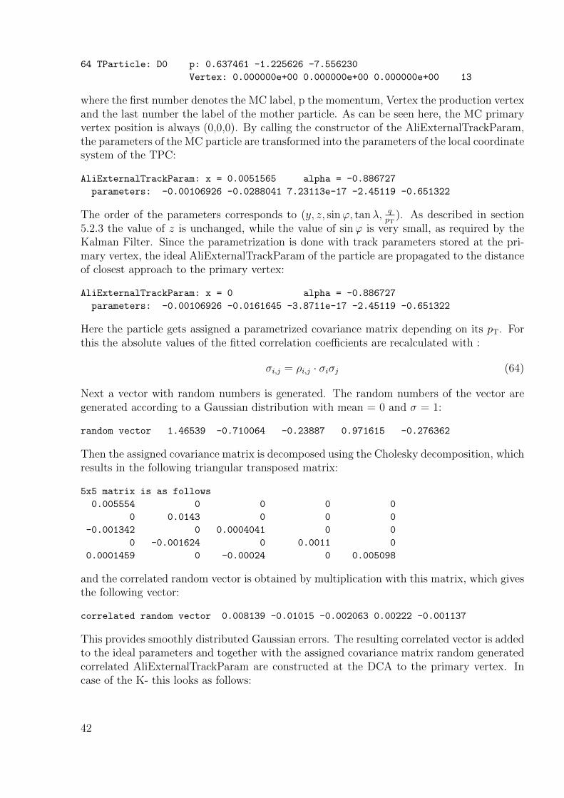
64 TParticle: D0 p: 0.637461 -1.225626 -7.556230

Vertex: 0.000000e+00 0.000000e+00 0.000000e+00 13

where the first number denotes the MC label, p the momentum, Vertex the production vertexand the last number the label of the mother particle. As can be seen here, the MC primaryvertex position is always (0,0,0). By calling the constructor of the AliExternalTrackParam,the parameters of the MC particle are transformed into the parameters of the local coordinatesystem of the TPC:

AliExternalTrackParam: x = 0.0051565 alpha = -0.886727

parameters: -0.00106926 -0.0288041 7.23113e-17 -2.45119 -0.651322

The order of the parameters corresponds to (y, z, sinϕ, tanλ, qpT

). As described in section5.2.3 the value of z is unchanged, while the value of sinϕ is very small, as required by theKalman Filter. Since the parametrization is done with track parameters stored at the pri-mary vertex, the ideal AliExternalTrackParam of the particle are propagated to the distanceof closest approach to the primary vertex:

AliExternalTrackParam: x = 0 alpha = -0.886727

parameters: -0.00106926 -0.0161645 -3.8711e-17 -2.45119 -0.651322

Here the particle gets assigned a parametrized covariance matrix depending on its pT. Forthis the absolute values of the fitted correlation coefficients are recalculated with :

σi,j = ρi,j · σiσj (64)

Next a vector with random numbers is generated. The random numbers of the vector aregenerated according to a Gaussian distribution with mean = 0 and σ = 1:

random vector 1.46539 -0.710064 -0.23887 0.971615 -0.276362

Then the assigned covariance matrix is decomposed using the Cholesky decomposition, whichresults in the following triangular transposed matrix:

5x5 matrix is as follows

0.005554 0 0 0 0

0 0.0143 0 0 0

-0.001342 0 0.0004041 0 0

0 -0.001624 0 0.0011 0

0.0001459 0 -0.00024 0 0.005098

and the correlated random vector is obtained by multiplication with this matrix, which givesthe following vector:

correlated random vector 0.008139 -0.01015 -0.002063 0.00222 -0.001137

This provides smoothly distributed Gaussian errors. The resulting correlated vector is addedto the ideal parameters and together with the assigned covariance matrix random generatedcorrelated AliExternalTrackParam are constructed at the DCA to the primary vertex. Incase of the K- this looks as follows:

42

AliExternalTrackParam: x = 0 alpha = -0.886727

parameters: 0.00707018 -0.0263203 -0.00206316 -2.44897 -0.65246

covariance: 3.085e-05

0 0.0002045

-7.452e-06 0 1.964e-06

0 -2.322e-05 0 3.846e-06

8.103e-07 0 -2.928e-07 0 2.607e-05

By calculating all correlation coefficients one gets the parametrized normalized covariancematrix:

Parametrized normalized covariance matrix:

5x5 matrix is as follows

| 0 | 1 | 2 | 3 | 4 |

----------------------------------------------------------------------

0 | 1 0 -0.9575 0 0.02857

1 | 0 1 0 -0.8278 0

2 | -0.9575 0 1 0 -0.04091

3 | 0 -0.8278 0 1 0

4 | 0.02857 0 -0.04091 0 1

0

20

40

60

80

100

120

140

160

z (cm)-0.08 -0.06 -0.04 -0.02 0 0.02 0.04

)λta

n(

-2.46

-2.455

-2.45

-2.445

-2.44

-2.435

-2.43

) without decompositionλCorrelation z, tan(

Entries 100000Mean x -0.0162Mean y -2.451RMS x 0.01436RMS y 0.001964

Correlation: -0.003069

) without decompositionλCorrelation z, tan(

(a) Example for a random Gaussian smearingwithout correlation.

0

50

100

150

200

250

300

z (cm)-0.08 -0.06 -0.04 -0.02 0 0.02 0.04

)λta

n(

-2.46

-2.455

-2.45

-2.445

-2.44

-2.435

-2.43

) with Cholesky decompositionλCorrelation z, tan(

Entries 100000Mean x -0.01615Mean y -2.451RMS x 0.01437RMS y 0.001972

Correlation: -0.828222

) with Cholesky decompositionλCorrelation z, tan(

(b) Example for a random correlated Gaussiansmearing using a Cholesky decomposition.

Figure 23

As a cross-check whether the parameters are correlated according to the input parameters,100.000 random correlated AliExternalTrackParam are generated from the example K-. Tocompare the effect of the multiplication with the decomposed matrix, the same smearing isdone for the K- without the Cholesky decomposition, which means that a random Gaussianvector with 0 mean and σ of the respective covariance matrix element is added to the idealAliExternalTrackParam (fig. 23a). For each of the AliExternalTrackParam, the value of z isplotted against the dip angle tanλ. Comparing the correlation coefficient σCtanλ = −0.8278with the correlation value of the histogram σTH2F

tanλ = −0.82822 (fig. 23b) one can see, that themultiplication of the random vector with the decomposed matrix correlates the parameters

43

according to the correlation coefficients given in the covariance matrix. Comparing the meanvalues and the RMS shows that the mean value is equal to the value of the respective elementin the ideal ExternalTrackParam and the RMS is equal to the square root of the respectivecovariance matrix element.

6.7 Definition of the test cases

In order to test and verify the algorithmic implementation of the code, the following observ-ables are implemented as test cases:

• reconstructed spatial position of the secondary vertex

• reconstructed transverse momentum of the mother

• reconstructed invariant mass of the mother

To quantify the precision of the reconstructed observables, the resolution is plotted againstpT, since all of the chosen observables have a pT dependence. The resolution of an observableX is defined as the width of the distribution of the reconstructed values minus the MonteCarlo values, which is expected to be Gaussian:

Resolution = σ(Xrec −XMC) (65)

In figure 24a an example for a pT integrated resolution of the position in x of a secondaryvertex is shown. One can see, that it is an overlap of many Gaussian functions. This is dueto the pT dependence. Therefore all checks for the resolution are made in pT bins. The meanvalue of the resolution has to be zero. To investigate, whether there is a bias, the mean valueof the distribution of the MC values minus the reconstructed values is plotted against pT.This is defined as the delta of the observable:

Delta = mean(Xrec −XMC) (66)

To have a check whether the errors of the observables are well estimated, the pull distributionis plotted. This is defined as the Gaussian width of the reconstructed value minus the Monte-Carlo value divided by the reconstructed error on that variable:

Pull = σ

(Xrec −XMC

σrecX

)(67)

Since the difference between the reconstructed and the Monte Carlo values should be coveredby the errors, the pull is expected to be a normal Gaussian distribution with zero meanand width equal to unity. An example for a pull distribution is shown in figure 24b. Toinvestigate whether the estimation of the errors is biased, the width of the pull is plotted overpT. The resolution, delta and pull are plotted for the different constraints of the KF: the massconstraint and the vertex constraint. To have a comparison with the vertexing tool recentlyused in ALICE, the secondary vertex is also reconstructed with the class AliVertexerTracks,which is typically used in the HF analysis. For the invariant mass, the common four vectoraddition serves as a comparison. Another important test is the χ2/ndf distribution of thevertex fits, where ndf denotes the number of degrees of freedom. Its mean value is expected

44

Entries 1551512Underflow 8058Overflow 7843Constant 7.004e+04Mean -1.162e-06Sigma 0.008119

(cm)MC - xrecx-0.04 -0.02 0 0.02 0.04

coun

ts

0

10000

20000

30000

40000

50000

60000

70000

80000

90000 Entries 1551512Underflow 8058Overflow 7843Constant 7.004e+04Mean -1.162e-06Sigma 0.008119

integratedT

Secondary vertex x resolution p

(a) Example for a resolution of the position in xof a secondary vertex.

Constant 1.481e+05

Mean -0.0001092

Sigma 1.003

recxσ

MC - xrecx-6 -4 -2 0 2 4 6

coun

ts

0

20

40

60

80

100

120

140

310×

Constant 1.481e+05

Mean -0.0001092

Sigma 1.003

integratedT

Secondary vertex x pull p

(b) Example for a pull distribution of the posi-tion in x of a secondary vertex.

Figure 24

to be unity and is related to the sum of the pulls. The probability distribution of the χ2

and the ndf has to be a flat distribution between zero and one. A mean value of the χ2/ndfdistribution that is higher than one indicates an underestimation of the errors of the fitand the probability is expected to increase towards zero, while a mean value of the χ2/ndfdistribution smaller than one indicates an overestimation of the errors and the probabilitydistribution is expected to increase towards one.

45

7 Test Results of AliKFParticle

7.1 Quality of the daughters

In order to make statements about the performance of the vertexing software, it is crucialto check the quality of the daughter tracks. To verify the results of the fast simulation thesame plots are made with the full Monte Carlo simulation on the sample LHC10f7a d, whichis a sample with added HF signals. This means that the production of heavy flavour in thecollision is artificially enhanced. The sample LHC10f7a d simulates proton-proton collisionsand is one of the main sources for the HF analysis in ALICE. In general the full simulationprovides a realistic simulation of the respective run of the real data. In the full simulationthe whole detector material is taken into account. The traversing of the material by theparticles is simulated with GEANT. For the analysis which uses the full simulation 6 ITSlayers and at least 70 TPC clusters are required for the daughter tracks. Besides a TPCand ITS refit, a χ2 < 4 cut for the TPC clusters is applied. To obtain the resolution ofthe daughter tracks, the tracks are propagated to the DCA to the MC decay vertex of themother particle. The comparison of the resolution of the track of the kaon as a function

(GeV/c)T

p0 2 4 6 8 10 12 14

) (c

m)

Rec

o -

pos

MC

(pos

σ

0

0.005

0.01

0.015

0.02

0.025

0.03

0.035

)Reco

- posMC

(posσRes kaon at decay vtx:

Resolution x

Resolution y

Resolution z Fast sim pp

)Reco

- posMC

(posσRes kaon at decay vtx:

(a) Spatial resolution in x, y, z of the kaon trackas a function of pT in global coordinates atthe decay vertex in the fast simulation. Thered points are hidden under the green points.

(GeV/c)T

p0 2 4 6 8 10 12 14

) (c

m)

Rec

o -

pos

MC

(pos

σ

0

0.005

0.01

0.015

0.02

0.025

0.03

0.035

)Reco

- posMC

(posσRes kaon at decay vtx:

Resolution x

Resolution y

Resolution z

Full sim pp

)Reco

- posMC

(posσRes kaon at decay vtx:

(b) Spatial resolution in x,y,z of the kaon trackas a function of its pT in global coordinatesat the decay vertex in the full simulation.

Figure 25

of its pT in the fast simulation with the full simulation (fig. 25a and 25b) shows, that theresolution of the kaon in the fast simulation at the MC decay vertex is in good agreementwith the full simulation, except in the first pT bin. Here the resolution in the fast simulationis too low.The resolution in z is worse than in x and y, which is not surprising, since the resolution ofthe detector in z is worse compared to the resolution in the transverse plane. The resolutionsof x and y are expected to be the same. This can be observed in the fast simulation, while inthe full simulation there is an asymmetry between x and y. The reason for this asymmetryis not understood yet and possibly only a feature of the sample LHC10f7a d.

As required the pulls of the fast simulation (fig. 26a) are very close to unity. This isvery important, since now the pulls of the reconstructed observables have to be also one

46

(GeV/c)T

p0 2 4 6 8 10 12 14

))R

eco

(pos

σ)/

Rec

o -

pos

MC

((po

sσ

0.97

0.98

0.99

1

1.01

1.02

1.03

Pull x

Pull y

Pull z Fast sim pp

))Reco

(posσ)/Reco

- posMC

((posσPull kaon at decay vtx:

(a) Pulls of the kaon track as a function of its pTat the MC decay vertex in x, y, z in the fastsimulation.

(GeV/c)T

p0 2 4 6 8 10 12 14

))R

eco

(pos

σ)/

Rec

o -

pos

MC

((po

sσ

0.7

0.75

0.8

0.85

0.9

0.95

1

1.05

1.1

1.15

1.2

Pull x

Pull y

Pull z

Full sim pp

))Reco

(posσ)/Reco

- posMC

((posσPull kaon at decay vtx:

(b) Pulls of the kaon track as a function of its pTat the MC decay vertex in x, y, z in the fullsimulation.

Figure 26

and, if not, indicate that there is an issue with the implemented code. In the last pT binthere is a deviation of about 2 %. Here higher statistics would be needed in order to checkwhether there is a small trend in the pulls of the fast simulation to overestimate the errorsfor increasing pT. The pulls of the full simulation (fig. 26b) show, that the errors of thetracks are approximately overestimated by 20 % . Therefore the errors of the reconstructedvalues for the secondary vertex in the full simulation are expected to be also overestimated.

7.2 Reconstruction of the D0

7.2.1 Secondary vertex

The secondary vertex is reconstructed from the two ESD tracks of the kaon and the pion.As described in chapter 6.7, the secondary vertex is reconstructed with the ALICE vertexingtool AliVertexerTracks. The exact functionality used in AliVertexerTracks isAliVertexerTracks::VertexForSelectedTracks. This functionality is used in the recent HFanalysis to reconstruct secondary vertices. It is required that the reconstructed vertex hastwo contributors and is inside the beam pipe. These cuts are applied to have consistencywith the cuts used in the HF analysis.

Figure 27a shows the resolution as a function of pT of AliVertexerTracks and of AliKF withthe two constraints in the fast simulation. AliKF gives a slightly better resolution than theAliVertexerTracks. The mass constraint gives only a very small improvement compared tothe unconstrained AliKF. A strong improvement, especially in the low pT range is obtained byconstraining the reconstructed particle to the MC primary vertex. Comparing this plot to theplot of the full simulation (fig. 27b) shows that here the topological constraint is significantlyworse and gives even worse results than the unconstrained fits for transverse momenta higherthan ≈ 2.5 GeV/c. The reason for this is, that in the case of the full simulation the particleis constrained to the ESD primary vertex that has an uncertainty. This shows that theresults of the resolution with the topological constraint depend strongly on the precision ofthe primary vertex. Therefore the topological constraint will be investigated in detail in

47

(GeV/c)T

p0 2 4 6 8 10 12 14

) (c

m)

Rec

o -

xM

C(xσ

0

0.002

0.004

0.006

0.008

0.01

0.012

0.014

0.016

0.018

0.02

)Reco - xMC

(xσResolution x decay vertex:

AliVertexerTracksAliKFAliKF mass constrainedAliKF topo constrained

Fast sim pp

)Reco - xMC

(xσResolution x decay vertex:

(a) Resolution in x of the position of the decayvertex of the D0 as a function of its pT inthe fast simulation. For the topological con-straint the MC primary vertex is used.

(GeV/c)T

p0 2 4 6 8 10 12 14

) (c

m)

Rec

o -

xM

C(xσ

0

0.002

0.004

0.006

0.008

0.01

0.012

0.014

0.016

0.018

0.02

)Reco - xMC

(xσResolution x decay vertex:

AliVertexerTracksAliKFAliKF massAliKF topo

Full sim pp

)Reco - xMC

(xσResolution x decay vertex:

(b) Resolution in x of the position of the decayvertex of the D0 as a function of its pT inthe full simulation. For the topological con-straint the ESD primary vertex is used.

Figure 27

chapter 9.3.Another important information is that all resolutions of the different vertex fits in the fastsimulation show qualitatively the same behaviour as the fits in the fast simulations whichconfirms that the fast simulation gives reliable results. The statistics of the full simulation islimited, so that no quantitative statements about the difference in the vertexing performancebetween the AliVertexerTracks, unconstrained AliKF and mass constrained AliKF can bemade.

(GeV/c)T

p0 2 4 6 8 10 12 14

) (c

m)

Rec

o -

zM

C(zσ

0

0.002

0.004

0.006

0.008

0.01

0.012

0.014

0.016

0.018

0.02

AliVertexerTracksAliKFAliKF mass constrainedAliKF topo constrained

Fast sim pp

)Reco - zMC

(zσResolution z decay vertex:

(a) Resolution of the position in z of the decayvertex of the D0 as a function of its pT in thefast simulation.

(GeV/c)T

p0 2 4 6 8 10 12 14

mea

n an

gle

(deg

)

0

0.5

1

1.5

2

2.5

3

Full sim pp

Opening angle in space with AliKF

(b) Opening angle between the kaon and thepion as a function of the pT of the D0 inthe full simulation with AliKF.

Figure 28

In z (fig. 28a) the resolution is slightly improved by the mass constraint compared to theAliVertexerTracks in the fast simulation. Also here a significant improvement is obtained byconstraining the particle to the MC primary vertex. Although the resolution of the daughtertracks in z is factors worse than the resolution in x, the resolution of the secondary vertex

48

in z is never more than a factor 2 worse than the resolution in x.The behaviour of the resolution of AliVertexerTracks, the unconstrained AliKF and the massconstrained AliKF is dominated by the resolution of the daughters and the opening anglebetween the daughters. The vertexing algorithms get more precise results when the openingangle between the daughters is larger. Therefore the resolution of the secondary vertex isworse in the low pT region due to the worse resolution of the daughters and also gets worsein the high pT region due to the decreasing opening angle. The opening angle obtained withAliKF in the full simulation is shown in figure 28b. The best resolution is obtained for a pTbetween 3 GeV/c and 4 GeV/c, where both effects are moderate.

The pulls of the position of the secondary vertex reconstruction show that the errors

(GeV/c)T

p0 2 4 6 8 10 12 14

)R

eco

xσ)/

Rec

o -

xM

C((

xσ

0.9

0.95

1

1.05

1.1

1.15

1.2

1.25

1.3

1.35

1.4

)Recoxσ)/Reco - x

MC((xσPull x decay vertex:

AliVertexerTracksAliKFAliKF mass constrainedAliKF topo constrained

Fast sim pp

)Recoxσ)/Reco - x

MC((xσPull x decay vertex:

(a) Pull of the position of the decay vertex in xas a function of the pT of the D0 in the fastsimulation.

(GeV/c)T

p0 2 4 6 8 10 12 14

)R

eco

xσ)/

Rec

o -

xM

C((

xσ

0.7

0.8

0.9

1

1.1

1.2

1.3

AliVertexerTracksAliKFAliKF massAliKF topo

)Recoxσ)/Reco - x

MC((xσPull x decay vertex:

Full sim pp

(b) Pull of the position of the decay vertex in xas a function of the pT of the D0 in the fullsimulation.

Figure 29

of the AliKF are well estimated. In the fast simulation (fig. 29a) one can see that thepulls of the AliKF and the AliKF mass constrained are, as expected, close to unity, whilethe pull of the AliKF topological constraint differs by 5 %, which is still acceptable. TheAliVertexerTracks shows a behaviour that is not understood yet. In the fast simulation ithas a bias towards larger pT. Since the pulls of the daughters in the full simulation wereabout 0.8, the pulls of the reconstructed vertex are expected to also be around this value.This is the case for the AliKF and also for the AliKF mass constrained (fig. 29b). The pullof the topological constraint shows qualitatively the same behaviour as in the fast simulationand is also too high. However, the AliVertexerTracks shows no bias in the full simulationand gives pulls that are very close to unity. The difference between the behaviour in the fastsimulation and in the full simulation of this tool should be checked in the future, especiallywhy AliVertexerTracks gives perfect pulls, although the daughter errors are overestimated.The mean values of the vertex position as a function of pT (fig. 30a, 30b) show that thereis no bias in the reconstruction of the vertex. The values are distributed randomly aroundthe true MC positions for both the fast and the full simulation.

49

(GeV/c)T

p0 2 4 6 8 10 12 14

)R

eco

- x

MC

mea

n(x

-0.1

-0.05

0

0.05

0.1

0.15

0.2

0.25

0.3-310×

AliVertexerTracksAliKFAliKF mass constrainedAliKF topo constrained

Fast sim pp

)Reco - xMC

Delta x decay vertex: mean(x

(a) Delta of the position of the decay vertex in xas a function of the pT of the D0 in the fastsimulation.

(GeV/c)T

p0 2 4 6 8 10 12 14

)R

eco

- x

MC

mea

n(x

-0.002

-0.0015

-0.001

-0.0005

0

0.0005

0.001

0.0015

0.002

0.0025

0.003

AliVertexerTracksAliKFAliKF mass constrainedAliKF topo constrained

Full sim pp

)Reco - xMC

Delta x decay vertex: mean(x

(b) Delta of the position of the decay vertex in xas a function of the pT of the D0 in the fastsimulation.

Figure 30

7.2.2 χ2/ndf and probability

For the unconstrained AliKF vertex fit and for the two constrained vertex fits the distri-butions of the χ2/ndf and the probability are investigated. As comparison also AliVertex-erTracks is shown. For the fast simulation the χ2/ndf distribution is expected to have amean value of one, while for the full simulation the mean value of the χ2/ndf distribution isexpected to be approximately 0.8, since the errors of the daughters are 20 % overestimatedwhich should reflect in the mean value of the χ2/ndf distribution. The distribution of

/ndf2χ0 1 2 3 4 5 6 7 8 9 10

coun

ts

310

410

510

Chi2 AliVertexer

Mean: 1.414534

AliVertexer

Fast pp

Chi2 AliVertexer

/ndf2χ0 2 4 6 8 10 12 14 16 18 20

coun

ts

1

10

210

310

410

510

610

Chi2 AliKF

Mean: 0.999577

AliKF

Fast pp

Chi2 AliKF

/ndf2χ0 2 4 6 8 10 12 14 16 18 20

coun

ts

1

10

210

310

410

510

Chi2 AliKF mass

Mean: 1.001774

AliKF mass

Fast pp

Chi2 AliKF mass

/ndf2χ0 2 4 6 8 10 12 14 16 18 20

coun

ts

310

410

510

Chi2 AliKF topo

Mean: 1.307079AliKF topo

Fast pp

Chi2 AliKF topo

prob0 0.1 0.2 0.3 0.4 0.5 0.6 0.7 0.8 0.9 10

2000

4000

6000

8000

10000

12000

14000

16000

18000

20000

Prob AliVertexer

Prob AliVertexer

Fast pp

Prob AliVertexer

prob0 0.1 0.2 0.3 0.4 0.5 0.6 0.7 0.8 0.9 10

2000

4000

6000

8000

10000

12000

14000

16000

18000

20000

Prob AliKF

Prob AliKF

Fast pp

Prob AliKF

prob0 0.1 0.2 0.3 0.4 0.5 0.6 0.7 0.8 0.9 10

2000

4000

6000

8000

10000

12000

14000

16000

18000

20000

Prob AliKF mass

Prob AliKF mass

Fast pp

Prob AliKF mass

prob0 0.1 0.2 0.3 0.4 0.5 0.6 0.7 0.8 0.9 10

2000

4000

6000

8000

10000

12000

14000

16000

18000

20000

Prob AliKF topo

Prob AliKF topo

Fast pp

Prob AliKF topo

Figure 31: The top panel shows the χ2/ndf distribution of the different vertexer in the fast simulation. Thebottom panel shows the respective probability distribution.

the χ2/ndf in the fast simulation is shown in figure 31 and confirms what has been seen inthe pulls of the resolution. The AliVertexerTracks underestimates the error and thus hasa mean value that is higher than one and the probability distribution increases in the first

50

/ndf2χ0 1 2 3 4 5 6 7 8 9 10

coun

ts

1

10

210

310

Chi2 AliVertexer

Mean: 1.047706

AliVertexer

Full pp

Chi2 AliVertexer

/ndf2χ0 1 2 3 4 5 6 7 8 9 10

coun

ts

1

10

210

310

Chi2 KF

Mean: 0.821903

AliKF

Full pp

Chi2 KF

/ndf2χ0 1 2 3 4 5 6 7 8 9 10

coun

ts

1

10

210

310

Chi2 KF mass const

Mean: 1.042272

AliKF mass

Full pp

Chi2 KF mass const

/ndf2χ0 1 2 3 4 5 6 7 8 9 10

coun

ts

1

10

210

310

Chi2 KF topo const

Mean: 1.694566AliKF topo

Full pp

Chi2 KF topo const

prob0 0.1 0.2 0.3 0.4 0.5 0.6 0.7 0.8 0.9 1

coun

ts

0

20

40

60

80

100

120

140

160

180

200

Prob AliVertexer

Prob AliVertexer

Full pp

Prob AliVertexer

prob0 0.1 0.2 0.3 0.4 0.5 0.6 0.7 0.8 0.9 1

coun

ts

0

20

40

60

80

100

120

140

160

180

200

Prob KF

Prob AliKF

Full pp

Prob KF

prob0 0.1 0.2 0.3 0.4 0.5 0.6 0.7 0.8 0.9 1

coun

ts

0

20

40

60

80

100

120

140

160

180

200

Prob KF mass const

Prob AliKF mass

Full pp

Prob KF mass const

prob0 0.1 0.2 0.3 0.4 0.5 0.6 0.7 0.8 0.9 1

coun

ts

0

20

40

60

80

100

120

140

160

180

200

Prob KF topo const

Prob AliKF topo

Full pp

Prob KF topo const

Figure 32: The top panel shows the χ2/ndf distribution of the different vertexer in the full simulation. Thebottom panel shows the respective probability distribution.

bins. The mean values of the χ2/ndf distributions of the unconstrained AliKF and the massconstrained fit are close to unity and their probability distributions are flat. The mean valueof the χ2/ndf distribution of the topological constraint shows that here the uncertainty isunderestimated, which also reflects in an increase of the probability distribution in the firstbins. The mean values of the χ2/ndf distributions of the vertexer in the full simulation areshown in figure 32 and also match with the observations made in the pulls of the resolution.AliVertexerTracks gives a perfect χ2/ndf distribution, although the errors of the daughtertracks are overestimated. The unconstrained AliKF fit reflects the overestimation of theerrors of the daughter in its χ2/ndf distribution. This is also reflected by an increase of theprobability distribution. The mean values of the χ2/ndf distributions of the mass constraintand the topological constraint are both too high. Especially the χ2/ndf distribution of thetopological constraint has to be checked in the future.

7.2.3 Transverse momentum

The transverse momentum reconstruction is a feature that actually none of the used ALICEtools can provide. The AliKF is the only vertexing package in ALICE that constructs thewhole mother particle. It is often convenient to plot the relative pT resolution:

precT − pMCT

pTrec(68)

The resolution of the AliKF for the unconstrained and the two constrained reconstructionswith the fast simulation are shown in figure 33a. The pT resolution depends on pT asdescribed in section 5.3. In the variable

σpTpT

the multiple scattering effect is a constant forhigh momenta and the detector uncertainty increases linear with pT, while for low momentathe multiple scattering effect becomes proportional to 1

pTbecause of the β dependence. This

behaviour can be observed well for the unconstrained fit and the constrained fits. The massconstraint improves the momentum resolution significantly. The same effects can be seen in

51

(GeV/c)T

p0 2 4 6 8 10 12 14

)R

eco

T)/

pR

eco

T -

pM

C

T((

pσ

0

0.005

0.01

0.015

0.02

0.025)Reco

T)/pReco

T - pMC

T((pσ resolution:

Tp

AliKF

AliKF mass constrained

AliKF topo constrained Fast sim pp

)Reco

T)/pReco

T - pMC

T((pσ resolution:

Tp

(a) Resolution of the transverse momentum ofthe D0 in the fast simulation.

(GeV/c)T

p0 2 4 6 8 10 12 14

)R

eco

T)/

pR

eco

T -

pM

C

T((

pσ

0

0.005

0.01

0.015

0.02

0.025)Reco

T)/pReco

T - pMC

T((pσ resolution:

Tp

Full sim ppAliKF

AliKF mass

AliKF topo

)Reco

T)/pReco

T - pMC

T((pσ resolution:

Tp

(b) Resolution of the transverse momentum ofthe D0 in the full simulation.

Figure 33

the full simulation (fig. 33b). In the full simulation the topological constraint gives slightlyworse results than the unconstrained fit.In the high-pT region, the resolution in the fast simulation is too high. This is not surprising,since in the parametrization of q

pTof the tracks (fig. 17b), the ϕ dependence is neglected and

as shown in the residuals the uncertainty of the transverse momenta in the high-pT regionis underestimated. Although no energy correction is made, the description provided by thefast simulation is consistent with the full simulation in the low-pT region.The pulls in the case of the fast and the full simulation are shown in figure 34a and 34b. In

(GeV/c)T

p0 2 4 6 8 10 12 14

)R

eco

Tpσ)/

Rec

oT

- p

MC

T((

pσ

0.98

0.99

1

1.01

1.02

1.03

1.04

1.05

AliKF

AliKF mass constrained

AliKF topo constrained Fast sim pp

)Reco

Tpσ)/Reco

T - pMC

T((pσ pull:

Tp

(a) Pulls of the transverse momentum of the D0

in the fast simulation.

(GeV/c)T

p0 2 4 6 8 10 12 14

)R

eco

Tpσ)/

Rec

oT

- p

MC

T((

pσ

0.8

0.9

1

1.1

1.2

1.3

1.4

1.5

1.6

1.7

AliKF

AliKF mass constrained

AliKF topo constrained

)Reco

Tpσ)/Reco

T - pMC

T((pσ pull:

Tp

Full sim pp

(b) Pulls of the transverse momentum of the D0

in the full simulation.

Figure 34

the fast simulation, the pulls of the fits are close to unity, as it is required in case of a correctalgorithmic implementation. The topological constraint deviates by about 5 percent, butthe errors are well estimated. In the full simulation the pull for the mass constraint is closeto unity. The pull in the case of the unconstrained fit has the same behaviour as the pullof the topological constraint. Both pulls show that the errors are overestimated by up to 30

52

(GeV/c)T

p0 2 4 6 8 10 12 14

)R

eco

T)/

pR

eco

T -

pM

C

Tm

ean(

(p

-0.2

-0.1

0

0.1

0.2

0.3

0.4

0.5

0.6

0.7

0.8-310×

AliKF

AliKF mass constrained

AliKF topo constrained

Fast sim pp

)Reco

T)/pReco

T - pMC

T delta: mean((p

Tp

(a) Delta of the transverse momentum of the D0

in the fast simulation.

(GeV/c)T

p0 2 4 6 8 10 12 14

)R

eco

T)/

pR

eco

T -

pM

C

Tm

ean(

(p

-0.002

-0.001

0

0.001

0.002

0.003

AliKF

AliKF mass constrained

AliKF topo constrained

)Reco

T)/pReco

T - pMC

T delta: mean((p

Tp

Full sim pp

(b) Delta of the transverse momentum of the D0

in the full simulation.

Figure 35

percent. In figure 35a and 35b the delta of the pT is plotted. It can be seen, that there is asmall bias in the fit with the mass constraint, both for the fast and for the full simulation.

7.2.4 Invariant mass

(GeV/c)T

p0 2 4 6 8 10 12 14

) (G

eV)

Rec

o-M

MC

(Mσ

0.008

0.01

0.012

0.014

0.016

0.018

0.02

0.022

0.024

0.026

)Reco-MMC

(MσMass resolution:

AliKF

AliKF topo constrained

4 vectors Fast sim pp

)Reco-MMC

(MσMass resolution:

(a) Resolution of the invariant mass of the D0

as a function of its pT in the fast simulation.The blue and red points are hidden under theorange points.

(GeV/c)T

p0 2 4 6 8 10 12 14

) (G

eV)

Rec

o-M

MC

(Mσ

0.008

0.01

0.012

0.014

0.016

0.018

0.02

0.022

0.024

0.026

)Reco-MMC

(MσMass resolution:

AliKF

AliKF topo

4 vector

Full sim pp

)Reco-MMC

(MσMass resolution:

(b) Resolution of the invariant mass of the D0 asa function of its pT in the full simulation.

Figure 36

For the invariant mass, the unconstrained fit, the topologically constrained fit and thecalculation by four vectors is compared. Since the mass constraint assumes a certain mass ofthe mother particle, no meaningful resolution and error can be calculated. The four vectorscalculation is done by estimating the energy of the daughter particles assuming their perfectMC mass and the momentum of the track:

E =√M2

MC + p2track (69)

53

The invariant mass of the mother is then obtained by adding the two four vectors of thedaughters (px, py, pz, E). The results of the resolution obtained with the different fits areshown in figure 36a and 36b. It can be seen that neither in the fast nor in the full simulationan improvement of the mass resolution can be seen using the AliKF. Moreover, it can beseen, that the description provided by the fast simulation is not in a good agreement withthe full simulation. However, both in the fast and in the full simulation a deteriorationof the resolution towards higher transversal momenta can be seen. Since the momentumplays a crucial role in the reconstruction of the invariant mass, it does not surprise that theresolution is too high in the fast simulation in the high-pT region, as it was also seen for thepT resolution.The pulls of both the constrained and unconstrained fit of the fast simulation in figure 37a

(GeV/c)T

p0 2 4 6 8 10 12 14

))R

eco

(Mσ)/

Rec

o-M

MC

((M

σ

0.96

0.98

1

1.02

1.04

1.06

1.08

1.1

1.12

1.14

AliKF

AliKF topo constrained Fast sim pp

))Reco

(Mσ)/Reco-MMC

((MσMass pull:

(a) Pull of the invariant mass of the D0 as a func-tion of its pT in the fast simulation. For thefour vectors no pull is calculated.

(GeV/c)T

p0 2 4 6 8 10 12 14

))R

eco

(Mσ)/

Rec

o-M

MC

((M

σ

0.7

0.8

0.9

1

1.1

1.2

1.3

1.4

1.5

1.6

AliKF

AliKF topo constrained

))Reco

(Mσ)/Reco-MMC

((MσMass pull:

Full sim pp

(b) Pull of the invariant mass of the D0 as afunction of its pT in the full simulation. Forthe four vectors no pull is calculated.

Figure 37

(GeV/c)T

p0 2 4 6 8 10 12 14

) (G

eV)

Rec

o-M

MC

mea

n(M

-0.4

-0.3

-0.2

-0.1

0

0.1

0.2

0.3-310×

AliKF

AliKF topo constrained

4 vectors

Fast sim pp

)Reco-MMC

Delta mass: mean(M

(a) Delta of the invariant mass of the D0 as afunction of its pT in the fast simulation.

(GeV/c)T

p0 2 4 6 8 10 12 14

) (G

eV)

Rec

o-M

MC

mea

n(M

-0.002

-0.0015

-0.001

-0.0005

0

0.0005

0.001

0.0015

0.002

AliKF

AliKF topo constrained

4 vectors

)Reco-MMC

Delta mass: mean(M

Full sim pp

(b) Delta of the invariant mass of the D0 as afunction of its pT in the full simulation.

Figure 38

are close to unity. As for the previous observables, the pull of the topological constraint

54

deviates by about 5 percent. The errors of the four vectors are not calculated, thereforeno pull is shown. In the full simulation in figure 37b the pulls show the same behaviouras the pulls of the transverse momenta. Again the behaviour of the unconstrained fit issimilar to the behaviour of the topological constraint. For the low momenta the errors areunderestimated by up to 15 percent, while for high momenta the pulls are overestimated byup to 20 percent. In figure 38a and 38b the deltas are shown. Both in the fast and the fullsimulation the invariant mass is slightly biased. Since this is also observed for the four vectorreconstruction, this seems not to be a problem of the AliKF, but seems to originate fromthe tracks themselves. However, the bias is small compared to the mass of the D0 which isapproximately 1, 8696± 0.0002 GeV , while the bias is in the order of a few MeV for the fullsimulation.

55

8 Test Results of KFParticle

(GeV/c)T

p0 2 4 6 8 10 12 14

) (c

m)

Rec

o -

xM

C(xσ

0

0.002

0.004

0.006

0.008

0.01

0.012

0.014

0.016

0.018

0.02

)Reco - xMC

(xσResolution x decay vertex:

AliVertexerTracks

KF

KF mass constrained

Fast sim pp

)Reco - xMC

(xσResolution x decay vertex:

(a) Resolution of the secondary vertex in x of theD0 in the fast simulation with KFParticle.

(GeV/c)T

p0 2 4 6 8 10 12 14

)R

eco

xσ)/

Rec

o -

xM

C((

xσ

0.9

0.95

1

1.05

1.1

1.15

1.2

1.25

1.3

1.35

1.4

)Recoxσ)/Reco - x

MC((xσPull x decay vertex:

AliVertexerTracks

KF

KF mass constrained

Fast sim pp

)Recoxσ)/Reco - x

MC((xσPull x decay vertex:

(b) Pull the secondary vertex in x of the D0 inthe fast simulation with KFParticle.

Figure 39

The same tests which were shown for the AliKFParticle are made also for the new unifiedversion of KFParticle. After the discovery of issues with the estimation of errors, the codehas been modified by the developers. Since the topological constraint of the unified versionis still under investigation, it is not shown. Moreover at the moment no AliROOT versionwhich includes the unified KFParticle version is available. Thus no comparison to the fullsimulation can be made and only the fast simulation is investigated. However, the resultsin the previous section showed, that the fast simulation is in good agreement with the fullsimulation for the secondary vertex reconstruction and the transverse momentum. In figure39a the resolution of the secondary vertex position in x calculated with the new KF versionis shown.

(GeV/c)T

p0 2 4 6 8 10 12 14

)R

eco

T)/

pR

eco

T -

pM

C

T((

pσ

0

0.005

0.01

0.015

0.02

0.025)Reco

T)/pReco

T - pMC

T((pσ resolution:

Tp

KF

KF mass constrained Fast sim pp

)Reco

T)/pReco

T - pMC

T((pσ resolution:

Tp

(a) Resolution of the transverse momentum ofthe D0 in the fast simulation with KFParti-cle.

(GeV/c)T

p0 2 4 6 8 10 12 14

)R

eco

Tpσ)/

Rec

oT

- p

MC

T((

pσ

0.95

1

1.05

1.1

1.15

1.2

1.25

KF

KF mass constrained Fast sim pp

)Reco

Tpσ)/Reco

T - pMC

T((pσ pull:

Tp

(b) Pull of the transverse momentum of the D0

in the fast simulation with KFParticle.

Figure 40

Comparing this to the results obtained with AliKF shows, that the results are matching. In

56

the high-pT region the KF is slightly worse than the AliKF. The pulls of the unconstrainedand the mass constrained fit in figure 39b are close to unity. This shows that after theimprovements of the code in the new unified version the errors are now well estimated.The results of the pT resolution are shown in figure 40a. For the transverse momentumresolution the results obtained with the KFParticle version are the same as the results withAliKFParticle. However, the pulls of the unified KFParticle version, shown in figure 40b,indicate that the errors calculated with KFParticle are underestimated, because the pull issignificantly too large. This behaviour has to be investigated in the future. The resolutionof the invariant mass is shown in figure 41a.

(GeV/c)T

p0 2 4 6 8 10 12 14

) (G

eV)

Rec

o-M

MC

(Mσ

0.008

0.01

0.012

0.014

0.016

0.018

0.02

0.022

0.024

0.026

)Reco-MMC

(MσMass resolution:

KF

4 vectors Fast sim pp

)Reco-MMC

(MσMass resolution:

(a) Resolution of the invariant mass of the D0 inthe fast simulation with KFParticle.

(GeV/c)T

p0 2 4 6 8 10 12 14

))R

eco

(Mσ)/

Rec

o-M

MC

((M

σ

0.96

0.98

1

1.02

1.04

1.06

1.08

1.1

1.12

1.14

KFFast sim pp

))Reco

(Mσ)/Reco-MMC

((MσMass pull:

(b) Pull of the invariant mass of the D0 in thefast simulation with KFParticle.

Figure 41

(GeV/c)T

p0 2 4 6 8 10 12 14

)R

eco

T)/

pR

eco

T -

pM

C

Tm

ean(

(p

-0.2

-0.1

0

0.1

0.2

0.3

0.4

0.5

0.6

0.7

0.8-310×

KF

KF mass constrainedFast sim pp

)Reco

T)/pReco

T - pMC

T delta: mean((p

Tp

(a) Delta of the transverse momentum in the fastsimulation with KFParticle.

(GeV/c)T

p0 2 4 6 8 10 12 14

) (G

eV)

Rec

o-M

MC

mea

n(M

-0.4

-0.3

-0.2

-0.1

0

0.1

0.2

0.3-310×

KF

4 vectorsFast sim pp

)Reco-MMC

Delta mass: mean(M

(b) Delta of the invariant mass in the fast simu-lation with KFParticle.

Figure 42

Also the mass resolution calculated with KFParticle gives the same results as the fits withAliKFParticle.The pull of the KF in figure 41b shows that the unconstrained fit estimates the errors onthe invariant mass well. As it was observed for the AliKF, the mass constraint for the pT is

57

slightly biased, as well as all calculations of the invariant mass as shown in figure 42.The last important checks are the distributions of the χ2/ ndf and the probability of thevertex fit. This is shown in figure 43 for the unconstrained and the mass constrained fit.Both the distribution of the χ2/ ndf and the probability indicate that the fit is not opti-mal. The mean value of the χ2/ ndf distribution is higher than unity which also reflectsin the probability. Compared to the distribution of the χ2/ ndf of the AliKF fit, this is adeterioration and has to be corrected in the future.

/ndf2χ0 2 4 6 8 10 12 14 16 18 20

coun

ts

10

210

310

410

510

Chi2 KF

Mean: 1.152895KF

Fast pp

Chi2 KF

prob0 0.1 0.2 0.3 0.4 0.5 0.6 0.7 0.8 0.9 1

0

2000

4000

6000

8000

10000

12000

14000

16000

18000

20000

Prob KF

Prob KF

Fast pp

Prob KF

/ndf2χ0 2 4 6 8 10 12 14 16 18 20

coun

ts

1

10

210

310

410

510

Chi2 KF mass

Mean: 1.354010KF mass

Fast pp

Chi2 KF mass

prob0 0.1 0.2 0.3 0.4 0.5 0.6 0.7 0.8 0.9 1

0

2000

4000

6000

8000

10000

12000

14000

16000

18000

20000

Prob KF mass

Prob KF mass

Fast pp

Prob KF mass

Figure 43: χ2/ ndf and probability of the unconstrained and the mass constrained fit with KFParticle.

58

9 Primary Vertex and Impact Parameter withAliKFParticle

LHC

10e1

2LH

C10

e13

LHC

11b1

0aLH

C11

b10a

_with

_SD

DLH

C11

b10b

LHC

11b1

0b_w

ith_S

DD

LHC

12b1

aLH

C12

b1a_

wS

DD

LHC

12b1

bLH

C12

b1b_

wS

DD

LHC

12b1

cLH

C12

b1c_

wS

DD

LHC

12f1

aLH

C12

f1b

LHC

12i3

LHC

10d1

LHC

10d2

LHC

10d4

aLH

C10

d4LH

C10

e20

LHC

10e2

1LH

C10

f6a

LHC

10f6

LHC

10f7

a_b

LHC

10f7

a_c

LHC

10f7

a_d

LHC

10f7

a_e

LHC

11b2

LHC

12a4

/ndf

2 χ

02

468

1012

1416

1820

/ndf MC_pp2χESD primary vertex

ESD - HF daughters

Multivertexer primary vertex

Multivertexer - HF daughters0.9TeV

2.76 TeV

7 TeV

Figure 44: Mean values of the χ2/ndf for all available MC pp samples at GSI with and without refit withthe Multivertexer.

The precision of the primary vertex plays a crucial role in the HF analysis. A great issuein this analysis is the inclusion of daughter tracks in the primary vertex, that come from HFdecays and thus worsen the resolution of the primary vertex because they are not originatingfrom it. The KF software provides powerful tools to correct the primary for these effects.Since the KF constructs the whole particle at the secondary vertex, it is possible to includethe HF particle in the primary vertex fit. The results of these operations will be investigatedin the following section.

9.1 Primary ESD vertex

During first tests of the quality of the primary it was seen, that the mean value of the χ2/ndfdistribution was systematically too high in the MC pp sample LHC10f7a d. Therefore allavailable MC samples and samples of real data at GSI have been checked for the spatialresolution, pulls and the mean values of the χ2/ndf distribution. This is shown in figure 44.Additionally it was checked how these values change when all HF daughters are removed viathe function AliVertexerTracks::RemoveTracksFromVertex. It is expected, that the χ2/ndfdistribution improves after the removing of the daughters, since the fit is closer to the truththen. However, it was seen, that the removal of the HF daughters gave no significant im-provement of the χ2/ndf distribution. Further investigations showed that many samples hadthe same problem. For Monte Carlo samples produced after a certain date in 2012 the mean

59

values of the χ2/ndf distributions are close to unity again. The reason for this is the imple-mentation of a new vertexing package, called the Multivertexer. It is possible to refit oldersamples with this tool. As shown in the figure, this solves the problems and gives meaningfulχ2/ndf distributions with mean of around unity again. Therefore it is recommended to refitESDEvents of older samples with: AliESDUtils::RefitESDtracks(ESDEvent,6).

9.2 Improvement of the resolution

For the MC sample LHC10f7a d it is investigated how the resolution of the primary vertexchanges by recalculating it with different functionalities. After the preliminary considerationsin the previous section, the original ESD primary vertex is refitted with the Multivertexer.For every D0 that comes from the primary vertex it is probable that there is a secondcharmed hadron coming from the creation of the charm anti-charm pair in the collision.Therefore as a first check all included heavy flavour daughters are removed from the primaryvertex . The second tested case is the removal of the daughters of only one side of thischarm anti-charm pair which is closer to realistic analysis situations. This means that forevery found D0 the pion and kaon are removed. This is done with the ALICE tool AliVer-texerTracks::RemoveTrackFromVertex and with the functionalities that AliKF provides torecalculate the primary. In the last tested case the daughters of the D0 are removed andthe D0 reconstructed with the AliKF is added to the primary vertex fit. The results are

Contributors

0 10 20 30 40 50

) (c

m)

Rec

o -

XM

C(Xσ

0.002

0.003

0.004

0.005

0.006

0.007

0.008

0.009

0.01

0.011

0.012

)Reco - XMC

(XσResolution x primary vertex:

ESD primaryESD primary -HFESD one sideAliKF remove daughtersAliKF add mom

)Reco - XMC

(XσResolution x primary vertex:

(a) Resolution of the primary vertex with AliKFin x in the full simulation after various recal-culations.

Contributors

0 10 20 30 40 50

) (c

m)

Rec

o -

XM

C(Xσ

0.0025

0.003

0.0035

0.004

0.0045

0.005

0.0055

ESD primaryESD primary -HFESD one sideAliKF remove daughtersAliKF add mom

)Reco - XMC

(XσResolution x primary vertex:

(b) 45a in a different scale.

Figure 45

presented in figure 45a and 45b. As can be seen, the resolution of the primary vertex isdepending on the contributors. Therefore, by removing the daughters only, the resolutionworsens, although the removed tracks are not originating from the primary vertex. Thiseffect is strongest, when all HF daughters are excluded. By removing only one side of thecharmed quark pair, the resolution is still worse, but it can be seen, that the AliKF providesbetter results than the ALICE tool. By adding the mother after the removal of the daughtersan improvement of the resolution is obtained although one contributor is lost. The delta ofthe primary vertices shows, that there is a bias in the primary vertex obtained with AliKF

60

after the removal of the daughters (fig. 46a). However, after the addition of the mother nobias is seen any more.Another interesting feature of the primary vertices can be seen in the point with the lowestnumber of contributors. Here the ESD vertices provide significantly better results. This isdue to the influence of the diamond constraint that gives additional information and thus isvery useful in the low contributors region. The improvement of the resolution by removingthe daughters and adding the mother has some important consequences for the resolutionof observables that are depending on the precision of the primary vertex. This will beinvestigated in the following sections.

9.3 The topological constraint

As already described in section 7.2.1 the topological constraint depends strongly on theprimary vertex precision. Thus the topological constraint is applied and tested again afterthe removal of the daughters and the addition of the mother. The spatial resolution isplotted again. For comparison the constraint to the ideal MC primary is also plotted. The

Contributors

0 10 20 30 40 50

) (c

m)

Rec

o -

xM

Cm

ean(

x

-0.0015

-0.001

-0.0005

0

0.0005

0.001

0.0015

)Reco - xMC

Delta ESD primary x: mean(x

ESD primaryESD primary -HFESD one sideAliKF remove daughtersAliKF add mom

)Reco - xMC

Delta ESD primary x: mean(x

(a) Delta of the different primary vertices.

(GeV/c)T

p0 2 4 6 8 10 12 14

) (c

m)

Rec

o -

xM

C(xσ

0

0.002

0.004

0.006

0.008

0.01

0.012

0.014

0.016

0.018

0.02

Resolution of the recalculated topological constraint

topo const to AliKF +mom

topo const to MC

AliKF normal

Resolution of the recalculated topological constraint

(b) Topological constraint to different primaryvertices.

Figure 46

results are shown in figure 46b. It can be seen that the topological constraint to the MCprimary shows qualitatively the same behaviour as the constraint to the MC vertex in thefast simulation in figure 27a. Comparing this to the result of the ESD primary vertex in thefull simulation obtained in this section, a significant improvement of the resolution can beseen. In the high-pT region the resolution is close to the ideal resolution obtained with theconstraint to the MC primary vertex. In the low-pT region the resolution is still better thanthe one of the unconstrained AliKF fit. Therefore it is mandatory to first remove daughtersand add the mother if the topological constraint is used.

9.4 Impact parameter

Another observable that provides very useful information for the HF analysis is the impactparameter of the daughter tracks to the primary vertex. This is equal to the DCA of the

61

daughters to the primary vertex and needs to be measured with very high precision. Tocalculate the resolution of the impact parameter, ideal ESD tracks are created from the MCdaughters. The DCA between the MC primary vertex and the ideal MC daughter track iscalculated, which gives the true MC impact parameter. The measured impact parameterreflects the uncertainty on the primary vertex and of the track. In figure 47 the results of

(GeV/c)T

p0 2 4 6 8 10 12 14

) (c

m)

Rec

o -

IPM

C(I

Pσ

0

0.001

0.002

0.003

0.004

0.005

0.006

0.007

0.008

0.009

0.01

ESD

AliKF remove daughters

AliKF add mom

)Reco - IPMC

(IPσResolution xy IP Kaon ESD primary:

Figure 47: Impact parameter in the xy plane to different primary vertices as a function of the track transversemomentum.

the impact parameter of the Kaon to the original ESD primary vertex, the AliKF vertexwith removed daughters of one side of the charm quark pair and the AliKF vertex withthe removed daughter and added D0 is presented. The plot shows that the resolution ofthe impact parameter depends very strongly on the resolution of the primary vertex. Asexpected, the resolution worsens with the removal of daughters, but improves significantlyafter the addition of the mother. In the low-pT region no improvement is seen. One possiblehypothesis for this is, that in this region the resolution is dominated by the track error.

62

10 Conclusion and Outlook

10.1 Test of AliKF

The tests have shown, that for the decay of the D0 the parameters are well estimated by theAliKF. The resolution of the position of the secondary vertex can be improved by applyingthe topological constraint after the removal of the daughter tracks and the addition of themother to the primary vertex fit. The resolution of the transverse momentum can be im-proved by the application of the mass constraint. The mean value of the χ2/ndf distributionof the topological constraint is significantly higher than unity, while the unconstrained fitprovides excellent results. An improvement in the resolution of the impact parameter can beobtained by improving the resolution of the primary vertex. Since the development of AliKFwill not be continued, the results of this test now serve as a benchmark for the debuggingof the new version.

10.2 Test of KF

After the debugging of the code by the authors, the new version of KFParticle now givespulls that are close to unity for the D0 decay in the fast simulation, except for the transversemomentum where the pull of the mass constraint is biased. The results for the resolutionsare mostly the same as the ones obtained with AliKF. The mean values of the χ2/ndfdistributions of the unconstrained fit and the constrained fit have to be checked again. Thetests that are made for the topological constraint for AliKF have to be done for the KF assoon as the debugging of the topological constraint is finished. Since KF will be the versionof the future it is mandatory to at least reach the same performance that AliKF can provideat the moment.

10.3 Further checks on the vertexer

In the future some more checks for the AliVertexerTracks, AliKF and KF are necessary.The first important check is, whether there are numerical problems when switching from the5x5 covariance matrix of the ALICE track model to the 6x6 covariance matrix of the KFmodel. Since in the latter representation one row of the covariance matrix is fully correlated,it is possible that eigenvalues of the covariance matrix get negative. This problem is alsorelevant for the switch from the local to the global system in ALICE. Another importanttest is, to reconstruct K0

s and Λ0 decays, since they decay much later and thus the vertexersare confronted with new challenges. Moreover, the secondary vertex reconstruction withAliVertexerTracks has to be investigated.

10.4 The Unit Test

The unit test is a powerful tool to verify the algorithmic implementation of the vertexingcode. The main purpose of the unit test - to have control over the input - is achievedalready with the simple parametrization. Small deviations from the predicted output in theideal case can be detected, as can be seen in the example of the mean value of the χ2/ndfdistribution of the KFParticle. It is planned to include a version of this test in AliROOT,

63

so that every new version of KF can be tested with the ideal input. Moreover, by makingcorrections for the various dependencies in the parametrization for the fast simulation, it ispossible to develop a performance test that also takes into account the special features ofthe ALICE detector. Another important step would be to include a step between the idealcase and the test with the full simulation by making the pulls of the ideal case not Gaussianany more, so it can be seen on which stage the behaviour of the pulls in the full simulationdeviates from the behaviour in the ideal case.

10.5 Planned physics analysis with KF

Figure 48: Sketch of a prompt and a feeddown D0 [27].

In figure 48 a sketch of a prompt D0 coming directly from the primary vertex and afeeddown D0 coming from a B decay is shown. The ratio of the prompt and feeddown D0,that is important for the determination of the charm cross section, has a large uncertainty.Since no existing methods can provide a precise measurement, this ratio is calculated fromtheory. Therefore the goal is to develop a reliable experimental method to measure thisratio. There are two crucial properties of feeddowns that are illustrated in the sketch andcan be exploited for the analysis. First the B meson flies approximately 500 microns andthe D0 approximately 150 microns. Second the prompt D0 points back directly to theprimary vertex, while the feeddown D0 that is produced in the decay of the B meson doesnot point directly to the primary. Therefore the D0 will be constructed with the mass andthe topological constraint from the pion and kaon daughters. The idea is that the χ2/ndf ofthe vertex fit and the pseudo proper decay length of the D0 give information whether theD0 originates from the primary or not, because the χ2/ndf should be deviating significantlyfrom unity if the particle does not point back to the primary and the pseudo proper decaylength should be too large. Thus it will be investigated whether it is possible to separateprompt and feeddown D0 on a single candidate base.

64

References

[1] R. Averbeck. “Heavy-flavor production in heavy-ion collisions and implications for theproperties of hot QCD matter”. In: Prog.Part.Nucl.Phys. 70 (2013), pp. 159–209. doi:10.1016/j.ppnp.2013.01.001.

[2] Christoph Berger. Elementarteilchenphysik. Springer, 2014.

[3] (ed.) Sarkar S., (ed.) Satz H., and (ed.) Sinha B. “The physics of the quark-gluonplasma”. In: Lect.Notes Phys. 785 (2010), pp. 1–369. doi: 10.1007/978- 3- 642-

02286-9.

[4] J. Schukraft. “Heavy Ion physics with the ALICE experiment at the CERN LHC”.ALICE Collaboration. In: Phil.Trans.Roy.Soc.Lond. A370 (2012), pp. 917–932. doi:10.1098/rsta.2011.0469. arXiv: 1109.4291 [hep-ex].

[5] P. Braun-Munzinger and J. Stachel. “The quest for the quark-gluon plasma”. In: Nature448 (2007), pp. 302–309. doi: 10.1038/nature06080.

[6] Betty Bezverkhny Abelev et al. “Performance of the ALICE experiment at the CERNLHC”. ALICE Collaboration. In: International Journal of Modern Physics A 29.24(2014), p. 1430044. doi: 10.1142/S0217751X14300440.

[7] K. Aamodt et al. “The ALICE experiment at the CERN LHC”. ALICE Collaboration.In: JINST 3 (2008), S08002. doi: 10.1088/1748-0221/3/08/S08002.

[8] F. Carminati et al. “ALICE: physics performance report, volume I”. ALICE Collabo-ration. In: Journal of Physics G: Nuclear and Particle Physics 30.11 (2004), p. 1517.

[9] B. Abelev et al. “Measurement of charm production at central rapidity in proton-proton collisions at

√s = 2.76 TeV”. ALICE Collaboration. In: Journal of High Energy

Physics 2012.7, 191 (2012). doi: 10.1007/JHEP07(2012)191. url: http://dx.doi.org/10.1007/JHEP07%282012%29191.

[10] B. Abelev et al. “Measurement of electrons from beauty hadron decays in pp collisionsat”. ALICE Collaboration. In: Physics Letters B 721.13 (2013), pp. 13 –23. issn:0370-2693. doi: http://dx.doi.org/10.1016/j.physletb.2013.01.069. url:http://www.sciencedirect.com/science/article/pii/S0370269313001275.

[11] Martin Volkl. “Measurement of beauty-hadron decay electrons in Pb–Pb collisions at√sNN = 2.76 TeV with ALICE”. ALICE Collaboration. In: (2014). arXiv: 1412.2670

[nucl-ex].

[12] MinJung Kweon. “Recent results on open heavy-flavour observables in relativistic nu-clear collisions”. ALICE Collaboration. In: Nucl.Phys. A931 (2014), pp. 155–164. doi:10.1016/j.nuclphysa.2014.08.080.

[13] Sergey Gorbunov [Frankfurt University]. “On-line reconstruction algorithms for theCBM and ALICE experiments ”. https://www-alt.gsi.de/documents/DOC-2013-Dec-21.html. PhD thesis. Mar. 2013.

[14] I. Kisel, I. Kulakov, and M. Zyzak. “Standalone First Level Event Selection Packagefor the CBM Experiment”. CBM. In: Nuclear Science, IEEE Transactions on 60.5(2013), pp. 3703–3708. issn: 0018-9499. doi: 10.1109/TNS.2013.2265276.

65

[15] S. Gorbunov and I. Kisel. “Reconstruction of decayed particles based on the Kalmanfilter”. CBM. In: (2007). CBM-SOFT-note-2007-003.

[16] R. Fruhwirth et al. Data Analysis Techniques For High Energy Physics. CambridgeUniversity Press, 2000.

[17] B. Alessandro et al. “ALICE: Physics performance report, volume II”. ALICE Collab-oration. In: Journal of Physics G: Nuclear and Particle Physics 32 (2006), pp. 1295–2040.

[18] P. Billoir. “ERROR PROPAGATION IN THE HELIX TRACK MODEL”. In: (1986).CERN-DELPHI 87-4, PROG 63.

[19] C. Grupen and B. Shwartz. Particle Detectors. Cambridge University Press, 2008.

[20] Yu Belikov, K. Safark, and B. Batyunya. “Kalman Filtering Application for TrackRecognition and Reconstruction in ALICE Tracking System”. ALICE Collaboration.In: (1997). ALICE-INT-1997-24, CERN-ALICE-INT-1997-24.

[21] A. Dainese and N. Carrer. “A parametrization of the Kalman Filter track reconstruc-tion in the ALICE TPC”. ALICE Collaboration. In: (2003). ALICE-INT-2003-011.

[22] Sigmund Brandt. Data Analysis. Springer, 1999.

[23] R.L. Gluckstern. “Uncertainties in track momentum and direction, due to multi-ple scattering and measurement errors”. In: Nuclear Instruments and Methods 24.0(1963), pp. 381 –389. issn: 0029-554X. doi: http://dx.doi.org/10.1016/0029-554X(63)90347-1. url: http://www.sciencedirect.com/science/article/pii/0029554X63903471.

[24] M. Valentan, M. Regler, and R. Fruhwirth. “Generalization of the Gluckstern formulasII: Multiple scattering and non-zero dip angles”. In: Nuclear Instruments and Methodsin Physics Research Section A: Accelerators, Spectrometers, Detectors and AssociatedEquipment 606.3 (2009), pp. 728 –742. issn: 0168-9002. doi: http://dx.doi.org/10.1016/j.nima.2009.05.024. url: http://www.sciencedirect.com/science/article/pii/S0168900209009474.

[25] T. Sjostrand, S. Mrenna, and P. Z. Skands. “PYTHIA 6.4 Physics and Manual”. In:JHEP 0605 (2006), p. 026. doi: 10.1088/1126-6708/2006/05/026. arXiv: hep-ph/0603175 [hep-ph].

[26] Mathworks. Matlab, Random Number Generation. url: http://de.mathworks.com/help/matlab/ref/randn.html;jsessionid=7e33e0d62cdb52b50443592cf946.

[27] Francesco Prino. Private Communication. 2015.

66

*Acknowledgements

First and foremost, I would like to thank Silvia Masciocchi for the excellent supervisionand the great encouragement during the last seven months. Then I would like to thankMarian Ivanov for the provision of many, many ideas and the support in the development ofthe code. Moreover, I am grateful to Johannes Stiller and Michael Winn for the help and forproofreading my thesis and to Klaus Reygers for reading and evaluating it. Furthermore Iwould like to thank Maksym Zyzak for the well working collaboration and Ruben Shahoyanfor the patient and precise explanations. Special thanks go to my family and friends for thesupport during the last months.

67

*Erklarung

Ich versichere, dass ich diese Arbeit selbststandig verfasst und keine anderen als die angegebe-nen Quellen und Hilfsmittel benutzt habe.

Heidelberg, den 17.03.2015,

Lukas Layer

68