department of energy technology receiver design
TRANSCRIPT

Receiver Design Methodologyfor Solar Tower Power Plants
Master Thesis
Joseph Stalin Maria Jebamalai
Department of Energy Technology
Supervisors:
Dipl.-Ing. Peter Schottl, Internal Supervisor, Fraunhofer ISE, Freiburg
Dr. Bjorn Laumert, External Supervisor, KTH Royal Institute of Technology
KTH School of Industrial Engineering and ManagementDepartment of Energy Technology
Division of Heat and Power TechnologySE - 100 44, Stockholm
August 2016

Master of Science Thesis EGI_2016: 070 MSC EKV1157
Receiver Design Methodology for Solar Tower Power Plants
Joseph Stalin Maria Jebamalai
Approved
16th August 2016
Examiner
Dr. Björn Laumert
Supervisor
Dipl.-Ing. Peter Schöttl
Dr. Björn Laumert Commissioner
Contact person
Dr. Björn Laumert

Abstract – Swedish Centrala solmottagarsystem (CRS) är på frammarsch på grund av deras höga koncentrationsfaktor och höga potential att minska kostnaderna genom att öka kapacitetsfaktorn av solkraftanläggningar med lagring. I CRS kraftanläggningar är solljuset fokuserat på mottagaren genom arrangemanget av tusentals speglar för att omvandla solstrålning till värme för att driva värmecykler. Solmottagare används för att överföra värmeflux från solen till arbetsmediet. Generellt arbetar solmottagare i driftpunkter med hög temperatur och därför genereras strålningsförluster. Vidare har solmottagaren en betydande påverkan på den totala kostnaden för kraftverket. Således har konstruktion och modellering av mottagaren en signifikant påverkan på kraftanläggningseffektivitet och kostnad. Målet med detta examensarbete är att utveckla en designmetodik för att beräkna geometrin hos solmottagaren och dess verkningsgrad. Denna designmetodik riktar sig främst till stora kraftverk i området 100 MWe, men även skalbarheten av designmetoden har studerats. Den utvecklade konstruktionsmetoden implementerades i in-house designverktyg devISEcrs som även integrerar andra moduler som modellerar solspegelfält, lagring och kraftblocket för att beräkna den totala kraftverksverkningsgraden. Designmodeller för de andra komponenterna är delvis redan implementerade, men de är modifierade och/eller utvidgade för att integrera den nya CRS mottagarmodellen. Slutligen har hela mottagarmodellen validerats genom att jämföra resultaten med testdata från litteraturen.
Abstract
Central Receiver Systems (CRS) are gaining momentum because of their high concentration andhigh potential to reduce costs by means of increasing the capacity factor of the plant with storage.In CRS plants, sunlight is focused onto the receiver by the arrangement of thousands of mirrors toconvert the solar radiation into heat to drive thermal cycles. Solar receivers are used to transferthe heat flux received from the solar field to the working fluid. Generally, solar receivers workin a high-temperature environment and are therefore subjected to different heat losses. Also, thereceiver has a notable impact on the total cost of the power plant. Thus, the design and modellingof the receiver has a significant influence on efficiency and the cost of the plant. The goal of themaster thesis is to develop a design methodology to calculate the geometry of the receiver andits efficiency. The design methodology is mainly aimed at large-scale power plants in the range of100 MWe, but also the scalability of the design method has been studied. The developed receiverdesign method is implemented in the in-house design tool devISEcrs and also it is integrated withother modules like solar field, storage and power block to calculate the overall efficiency of thepower plant. The design models for other components are partly already implemented, but theyare modified and/or extended according to the requirements of CRS plants. Finally, the entirereceiver design model is validated by comparing the results of test cases with the data from theliterature.
ii Receiver Design Methodology for Solar Tower Power Plants

Acknowledgement
I express my sincere gratitude to Fraunhofer Institute of Solar Energy Systems (ISE) and KTHRoyal Institute of Technology for providing this wonderful opportunity to carry out my masterthesis in Germany. It was an incredible experience for me as I have gained lots of knowledge onCSP power plants.
I would take this opportunity to thank my supervisor at Fraunhofer ISE, Dipl.-Ing. Peter Schottlfor his continuous guidance and knowledge sharing throughout the thesis. I extend my gratitudeto my academic supervisor, Dr. Bjorn Laumert for his support. Special thanks to KTH andFraunhofer ISE for providing financial support and all the necessary facilities.
I am also thankful to Anna Heimsath, Bernhard Seubert, Claudia Sutardhio, De Wet Van Rooyen,Pankaj Deo, Raymond Branke, Shaab Rohani and Thomas Fluri for their contributions and dis-cussion about the project. Furthermore, I would like to thank all the staff members who helpedme through all phases of my thesis.
Finally, I would like to thank my parents and my friends, Abhishek Srujan, Anand Bhaskaranand Sai Janani Ramachandran for their continuous support and motivation all days, especiallyduring my hard times.
Receiver Design Methodology for Solar Tower Power Plants iii

Contents
Contents iv
List of Figures vi
List of Tables viii
Nomenclature ix
1 Introduction 11.1 Solar Radiation . . . . . . . . . . . . . . . . . . . . . . . . . . . . . . . . . . . . . . 11.2 Concentrated Solar Power (CSP) . . . . . . . . . . . . . . . . . . . . . . . . . . . . 21.3 Central Receiver Systems (CRS) . . . . . . . . . . . . . . . . . . . . . . . . . . . . 41.4 Research Statement . . . . . . . . . . . . . . . . . . . . . . . . . . . . . . . . . . . 61.5 Thesis Overview . . . . . . . . . . . . . . . . . . . . . . . . . . . . . . . . . . . . . 7
2 Literature Review 82.1 Tubular Receivers . . . . . . . . . . . . . . . . . . . . . . . . . . . . . . . . . . . . 8
2.1.1 Water/Steam . . . . . . . . . . . . . . . . . . . . . . . . . . . . . . . . . . . 82.1.2 Molten Salt . . . . . . . . . . . . . . . . . . . . . . . . . . . . . . . . . . . . 92.1.3 Liquid Sodium . . . . . . . . . . . . . . . . . . . . . . . . . . . . . . . . . . 102.1.4 Sodium/Salt Binary . . . . . . . . . . . . . . . . . . . . . . . . . . . . . . . 10
2.2 Design Criteria . . . . . . . . . . . . . . . . . . . . . . . . . . . . . . . . . . . . . . 112.2.1 Receiver Design Methodology . . . . . . . . . . . . . . . . . . . . . . . . . . 112.2.2 Allowable Peak Flux Limit . . . . . . . . . . . . . . . . . . . . . . . . . . . 122.2.3 Receiver Sizing . . . . . . . . . . . . . . . . . . . . . . . . . . . . . . . . . . 132.2.4 Receiver Aspect Ratio . . . . . . . . . . . . . . . . . . . . . . . . . . . . . . 132.2.5 Tube Diameter Selection . . . . . . . . . . . . . . . . . . . . . . . . . . . . . 142.2.6 Fluid Flow Path Selection . . . . . . . . . . . . . . . . . . . . . . . . . . . . 142.2.7 Tower Sizing . . . . . . . . . . . . . . . . . . . . . . . . . . . . . . . . . . . 15
2.3 Cavity Specific Design Criteria . . . . . . . . . . . . . . . . . . . . . . . . . . . . . 152.3.1 Cavity Receiver Geometry . . . . . . . . . . . . . . . . . . . . . . . . . . . . 162.3.2 Cavity Opening Angle . . . . . . . . . . . . . . . . . . . . . . . . . . . . . . 162.3.3 Lip Height (Aperture-to-Total Height Ratio) . . . . . . . . . . . . . . . . . 162.3.4 Cavity Inclination . . . . . . . . . . . . . . . . . . . . . . . . . . . . . . . . 17
2.4 Heat Transfer Model . . . . . . . . . . . . . . . . . . . . . . . . . . . . . . . . . . . 172.4.1 External Receiver . . . . . . . . . . . . . . . . . . . . . . . . . . . . . . . . 182.4.2 Cavity Receiver . . . . . . . . . . . . . . . . . . . . . . . . . . . . . . . . . . 21
3 Design Methodology 253.1 Design Approach . . . . . . . . . . . . . . . . . . . . . . . . . . . . . . . . . . . . . 253.2 General Receiver Design Model . . . . . . . . . . . . . . . . . . . . . . . . . . . . . 27
3.2.1 Receiver Thermal Power . . . . . . . . . . . . . . . . . . . . . . . . . . . . . 273.2.2 Calculation of HTF Properties . . . . . . . . . . . . . . . . . . . . . . . . . 27
iv Receiver Design Methodology for Solar Tower Power Plants

CONTENTS
3.2.3 Receiver Sizing . . . . . . . . . . . . . . . . . . . . . . . . . . . . . . . . . . 273.2.4 Receiver Surface Temperature Calculation . . . . . . . . . . . . . . . . . . . 283.2.5 Mass Flow Rate Calculation . . . . . . . . . . . . . . . . . . . . . . . . . . . 293.2.6 Pressure Loss and Pump Power Calculation . . . . . . . . . . . . . . . . . . 29
3.3 External Receiver Design Model . . . . . . . . . . . . . . . . . . . . . . . . . . . . 303.3.1 Geometry Design . . . . . . . . . . . . . . . . . . . . . . . . . . . . . . . . . 303.3.2 Tube and Panel Design . . . . . . . . . . . . . . . . . . . . . . . . . . . . . 303.3.3 Tower Height Design . . . . . . . . . . . . . . . . . . . . . . . . . . . . . . . 323.3.4 Receiver Thermal Efficiency . . . . . . . . . . . . . . . . . . . . . . . . . . . 33
3.4 Cavity Receiver Design Model . . . . . . . . . . . . . . . . . . . . . . . . . . . . . . 343.4.1 Geometry Design . . . . . . . . . . . . . . . . . . . . . . . . . . . . . . . . . 343.4.2 Tube and Panel Design . . . . . . . . . . . . . . . . . . . . . . . . . . . . . 363.4.3 Tower Height Design . . . . . . . . . . . . . . . . . . . . . . . . . . . . . . . 363.4.4 Receiver Thermal Efficiency . . . . . . . . . . . . . . . . . . . . . . . . . . . 37
4 Implementation 394.1 devISEcrs - A Design Tool . . . . . . . . . . . . . . . . . . . . . . . . . . . . . . . 394.2 Implementation Structure . . . . . . . . . . . . . . . . . . . . . . . . . . . . . . . . 404.3 Interface of Receiver Classes . . . . . . . . . . . . . . . . . . . . . . . . . . . . . . . 41
4.3.1 Receiver Class . . . . . . . . . . . . . . . . . . . . . . . . . . . . . . . . . . 414.3.2 External Receiver Class . . . . . . . . . . . . . . . . . . . . . . . . . . . . . 414.3.3 Cavity Receiver Class . . . . . . . . . . . . . . . . . . . . . . . . . . . . . . 41
5 Validation and Results 445.1 Receiver Design Validation . . . . . . . . . . . . . . . . . . . . . . . . . . . . . . . 44
5.1.1 External Receiver . . . . . . . . . . . . . . . . . . . . . . . . . . . . . . . . 445.1.2 Cavity Receiver . . . . . . . . . . . . . . . . . . . . . . . . . . . . . . . . . . 48
5.2 Receiver Thermal Losses Validation . . . . . . . . . . . . . . . . . . . . . . . . . . 495.2.1 External Receiver . . . . . . . . . . . . . . . . . . . . . . . . . . . . . . . . 495.2.2 Cavity Receiver . . . . . . . . . . . . . . . . . . . . . . . . . . . . . . . . . . 50
5.3 Effect of Spillage Loss on Heliostat Size . . . . . . . . . . . . . . . . . . . . . . . . 51
6 Conclusion and Future Work 536.1 Conclusion . . . . . . . . . . . . . . . . . . . . . . . . . . . . . . . . . . . . . . . . 536.2 Future Work . . . . . . . . . . . . . . . . . . . . . . . . . . . . . . . . . . . . . . . 53
Bibliography 54
Receiver Design Methodology for Solar Tower Power Plants v

List of Figures
1.1 Direct, diffuse and reflected radiation [8] . . . . . . . . . . . . . . . . . . . . . . . . 1
1.2 World solar DNI map [50] . . . . . . . . . . . . . . . . . . . . . . . . . . . . . . . . 2
1.3 Example of solar thermal power plant with four subsystems [3] . . . . . . . . . . . 3
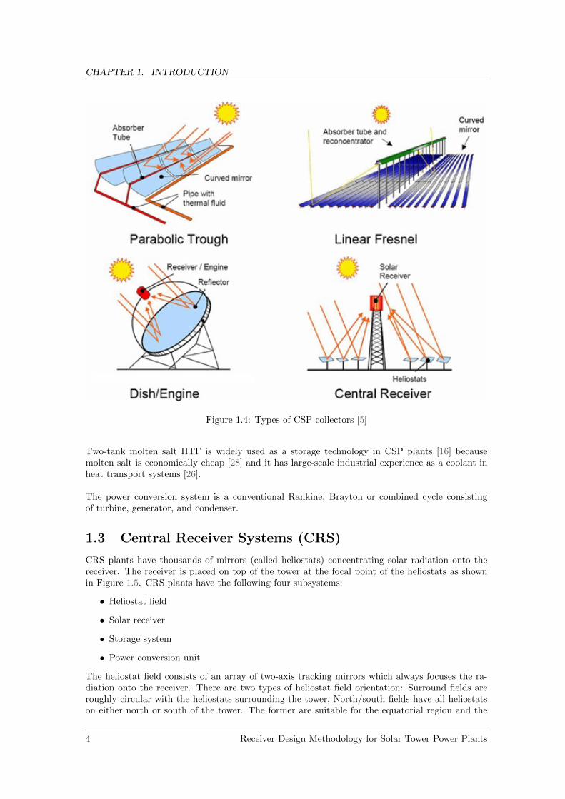
1.4 Types of CSP collectors [5] . . . . . . . . . . . . . . . . . . . . . . . . . . . . . . . 4
1.5 Gemasolar 20MW solar tower power plant in Sevilla, Spain [6] . . . . . . . . . . . 5
1.6 Optical losses in the heliostat field . . . . . . . . . . . . . . . . . . . . . . . . . . . 5
1.7 Solar receivers [9] . . . . . . . . . . . . . . . . . . . . . . . . . . . . . . . . . . . . . 6
2.1 Tubular receivers from Solar Two plant (left) and PS10 plant (right) [52] . . . . . 8
2.2 Flow layout of water/steam central receiver system [2] . . . . . . . . . . . . . . . . 9
2.3 Flow layout of molten salt central receiver system [52] . . . . . . . . . . . . . . . . 9
2.4 Flow layout of liquid sodium central receiver system [22] . . . . . . . . . . . . . . . 10
2.5 Flow layout of sodium/salt binary central receiver system [22] . . . . . . . . . . . . 11
2.6 Tubular receivers: a) External receiver, b) Cavity receiver [10] . . . . . . . . . . . . 11
2.7 Receiver peak flux value for different HTF and materials with respect to life cycles[22] . . . . . . . . . . . . . . . . . . . . . . . . . . . . . . . . . . . . . . . . . . . . . 13
2.8 Eight possible fluid flow configuration by Wagner [52] . . . . . . . . . . . . . . . . 14
2.9 Solar tower for external and cavity receivers [23] . . . . . . . . . . . . . . . . . . . 15
2.10 Cavity receiver geometry with four receiver panels [23] . . . . . . . . . . . . . . . . 16
2.11 Lip height of cavity receiver [33] . . . . . . . . . . . . . . . . . . . . . . . . . . . . 17
2.12 Cavity inclination angle [33] . . . . . . . . . . . . . . . . . . . . . . . . . . . . . . . 17
2.13 Variation of Richardson number with respect to wind velocity for cavity receiver [48] 22
2.14 Two-zone model of the cavity receiver [25] . . . . . . . . . . . . . . . . . . . . . . . 23
3.1 Receiver design methodology for tubular receivers . . . . . . . . . . . . . . . . . . . 26
3.2 External receiver geometry [45] . . . . . . . . . . . . . . . . . . . . . . . . . . . . . 30
3.3 Tube diameter correlation with respect to receiver thermal power . . . . . . . . . . 31
3.4 Variation of tower height with respect to receiver thermal power [22] . . . . . . . . 32
3.5 Tower height correlation with respect to receiver thermal power for external receiver 33
3.6 Geometry of cavity receiver [23] . . . . . . . . . . . . . . . . . . . . . . . . . . . . . 34
3.7 Internal angle geometry of cavity receiver [23] . . . . . . . . . . . . . . . . . . . . . 35
3.8 Tower height correlation with respect to receiver thermal power for cavity receiver 36
3.9 Internal heat transfer area of the cavity receiver [43] . . . . . . . . . . . . . . . . . 37
4.1 Modules of the devISEcrs design tool . . . . . . . . . . . . . . . . . . . . . . . . . . 39
4.2 Class inheritance structure of the receiver module in devISEcrs . . . . . . . . . . . 40
5.1 Total and individual loss component comparison for external receiver . . . . . . . . 50
5.2 Total and individual loss component comparison for cavity receiver . . . . . . . . . 51
5.3 External receiver spillage loss of different power plant sizes with respect to heliostatsize . . . . . . . . . . . . . . . . . . . . . . . . . . . . . . . . . . . . . . . . . . . . . 52
vi Receiver Design Methodology for Solar Tower Power Plants

LIST OF FIGURES
5.4 Cavity receiver spillage loss of different power plant sizes with respect to heliostatsize . . . . . . . . . . . . . . . . . . . . . . . . . . . . . . . . . . . . . . . . . . . . . 52
Receiver Design Methodology for Solar Tower Power Plants vii

List of Tables
2.1 Receiver flux limit for different HTF [22] . . . . . . . . . . . . . . . . . . . . . . . . 132.2 Nusselt correlation for forced convection of external receivers [43] . . . . . . . . . . 20
3.1 Properties of solar salt [55] . . . . . . . . . . . . . . . . . . . . . . . . . . . . . . . 273.2 Tube diameter used in various commercial power plants [49] [39] [51] . . . . . . . . 31
4.1 Input parameters and its default value of the receiver class . . . . . . . . . . . . . 414.2 Input parameters and its default value of the external receiver class . . . . . . . . . 424.3 Output parameters of the external receiver class . . . . . . . . . . . . . . . . . . . 424.4 Input parameters and its default value of the cavity receiver class . . . . . . . . . . 424.5 Output parameters of the cavity receiver class . . . . . . . . . . . . . . . . . . . . . 43
5.1 Solar Two power plant characteristics [51] . . . . . . . . . . . . . . . . . . . . . . . 455.2 Comparison of Solar Two receiver design parameters . . . . . . . . . . . . . . . . . 455.3 Gemasolar power plant characteristics [36] . . . . . . . . . . . . . . . . . . . . . . . 465.4 Comparison of Gemasolar receiver design parameters . . . . . . . . . . . . . . . . . 465.5 Crescent Dunes power plant characteristics [37] . . . . . . . . . . . . . . . . . . . . 475.6 Comparison of Crescent Dunes receiver design parameters . . . . . . . . . . . . . . 485.7 PS10 power plant characteristics [44] . . . . . . . . . . . . . . . . . . . . . . . . . . 485.8 Comparison of PS 10 receiver design parameters . . . . . . . . . . . . . . . . . . . 495.9 Validation of molten salt external receiver thermal losses . . . . . . . . . . . . . . . 495.10 Validation of molten salt cavity receiver thermal losses . . . . . . . . . . . . . . . . 50
viii Receiver Design Methodology for Solar Tower Power Plants

Nomenclature
Abbrevations
CRS Central Receiver Systems
CSP Concentrated Solar Power
DNI Direct Normal Irradiance
HTF Heat Transfer Fluid
Greek symbols
α Absorptance -
β Volumetric expansion coefficient 1/K
ε Emissivity -
η Efficiency -
µ Dynamic viscosity kg/ms
ν Kinematic viscosity m2/s
ρ Density kg/m3
σ Stefan-Boltzmann constant W/m2K4
θ Cavity opening angle -
Symbols
∆P Pressure difference N/m2
m Mass flow rate kg/s
Q Energy W
cp Specific heat J/kgK
Ks Surface roughness -
uwind Wind velocity m/s
qo Allowable peak flux W/m2
A Area m2
D Diameter m
d Diameter of the receiver tube m
Receiver Design Methodology for Solar Tower Power Plants ix

NOMENCLATURE
f Darcy friction factor -
g Acceleration due to gravity m/s2
Gr Grashof number -
H Height m
h Heat transfer coefficient W/m2 K
k Thermal conductivity W/m K
L Length m
n Count -
Nu Nusselt number -
P Pressure N/m2
Pr Prandtl number -
R Thermal Resistance K/W
r Radius m
Ra Rayleigh number -
Re Reynolds number -
Ri Richardson number -
SM Solar multiple -
T Temperature K
v Velocity m/s
W Width m
Subscripts
abs Absorber
amb Ambient
avg Average
c Characteristic
cond Conduction
conv Convection
eff Effective
el Electric
env Envelope
f Film
for Forced
htf Heat transfer fluid
x Receiver Design Methodology for Solar Tower Power Plants

NOMENCLATURE
i Inner
inc Incident
max Maximum
min Minimum
mix Mixed
nat Natural
o Outer
pb Power block
rad Radiation
rec Receiver
ref Reflection
s Surface
th Thermal
tot Total
tube Receiver tube
w Wall
Receiver Design Methodology for Solar Tower Power Plants xi

Chapter 1
Introduction
The growing global energy demand and environmental pollution urge humanity to focus on re-newable energy. In order to meet the increasing energy demand in a sustainable way, solar energyhas the potential to act as a future energy source. One challenge with solar energy is that it is avariable source of energy. This can be tackled with Concentrated Solar Power (CSP) coupled withstorage technology which assures dispatchability of energy. Hence, CSP can act as a promisingalternative source of energy in the future. CRS plant is one of the types of CSP plants, for whichthe receiver design methodology will be developed in this thesis. This chapter explains about basicconcepts of CSP technology, research statement and the thesis overview.
1.1 Solar Radiation
Figure 1.1: Direct, diffuse and reflected radiation [8]
Solar irradiance is the rate of radiant energy per unit area over a period of time produced from thesun. The units of solar irradiance are W/m2 [45] and suns. One sun is equal to 1000 W/m2. Theatmosphere scatters and absorbs some of the solar radiation that is incident on the earth surfacebefore reaching the ground. This is mainly due to the dust particles, gaseous molecules and cloudsin the atmosphere. The amount of solar radiation reflected, scattered and absorbed depends on
Receiver Design Methodology for Solar Tower Power Plants 1

CHAPTER 1. INTRODUCTION
Figure 1.2: World solar DNI map [50]
the distance travelled by the solar radiation, levels of dust particles and water vapour present inthe atmosphere. Figure 1.1 shows the three types of radiation which are explained below:
• Direct radiation - The radiation which is coming straight through the atmosphere withoutgetting scattered is called direct radiation and it is directional.
• Diffuse radiation - The radiation, which gets scattered by the particles and molecules in theatmosphere, but still made it down to the earth surface, is called diffuse radiation.
• Reflected radiation - The radiation which has been reflected due to obstacles such as buildingsand ground is called reflected radiation.
CSP plants convert only Direct Normal Irradiance (DNI) into electrical energy [14]. The minimumthreshold DNI necessary for the CSP technology is 2000 KWh/m2/year because of economicconstraints [14]. In order to have an idea about DNI, world solar DNI map is shown in the Figure1.2.
1.2 Concentrated Solar Power (CSP)
CSP technology mainly works on the principle of concentrating vast area direct insolation ontoabsorbers to convert it into thermal energy. Mirrors are used to focus the solar radiation ontoabsorbers. Absorbers are used to transfer the obtained solar thermal energy to a Heat TransferFluid (HTF). Then, the thermal energy in the HTF is used to generate steam and electricity isproduced by a conventional power cycle. Solar radiation is a variable source of energy, whichcannot be controlled. Thus, it is advisable to incorporate storage into the system. Consequently,CSP technology mainly consists of four subsystems [11] which are shown in the Figure 1.3:
2 Receiver Design Methodology for Solar Tower Power Plants

CHAPTER 1. INTRODUCTION
Figure 1.3: Example of solar thermal power plant with four subsystems [3]
• Solar collector/field
• Solar receiver
• Storage system
• Power conversion system
The solar collector mainly differs with the shape of the collector surface. There are line focusingsystems, which can be a parabolic trough or a linear fresnel collector, and point focusing systems,which can be a dish collector or a central receiver. The four types of commercially accomplishedCSP collectors [11] are depicted in Figure 1.4. Point focusing systems have a higher concentrationratio compared to the line focusing systems. Thus, higher temperatures can be easily achieved bypoint focusing systems [11].Solar receivers are the main focus of this thesis, therefore they are discussed in a separate section.The main technologies used in the storage system are sensible or latent heat storage. Some of thedifferent types of storage system are listed below:
• Storage systems
– Two-tank direct
– Two-tank indirect
– Single-tank thermocline
• Storage media
– Sensible heat storage
– Latent heat storage
Receiver Design Methodology for Solar Tower Power Plants 3
CHAPTER 1. INTRODUCTION
Figure 1.4: Types of CSP collectors [5]
Two-tank molten salt HTF is widely used as a storage technology in CSP plants [16] becausemolten salt is economically cheap [28] and it has large-scale industrial experience as a coolant inheat transport systems [26].
The power conversion system is a conventional Rankine, Brayton or combined cycle consistingof turbine, generator, and condenser.
1.3 Central Receiver Systems (CRS)
CRS plants have thousands of mirrors (called heliostats) concentrating solar radiation onto thereceiver. The receiver is placed on top of the tower at the focal point of the heliostats as shownin Figure 1.5. CRS plants have the following four subsystems:
• Heliostat field
• Solar receiver
• Storage system
• Power conversion unit
The heliostat field consists of an array of two-axis tracking mirrors which always focuses the ra-diation onto the receiver. There are two types of heliostat field orientation: Surround fields areroughly circular with the heliostats surrounding the tower, North/south fields have all heliostatson either north or south of the tower. The former are suitable for the equatorial region and the
4 Receiver Design Methodology for Solar Tower Power Plants

CHAPTER 1. INTRODUCTION
Figure 1.5: Gemasolar 20MW solar tower power plant in Sevilla, Spain [6]
latter are suitable for the northern/southern hemisphere due to the sun's path in the respectiveregion.
Solar radiation undergoes various optical losses before it reaches the receiver. Figure 1.6 de-picts various optical losses in the heliostat field. The cosine efficiency of the heliostat is the majoreffect which determines the optimum heliostat field layout [45]. This efficiency depends on boththe sun's position and the location of the individual heliostat relative to the receiver [45]. Thetracking mechanism is used to position the heliostat so that its surface normal bisects the anglebetween the sun's rays and the reflected radiation from the heliostat to the receiver. The effectivereflection area of the heliostat is reduced by the cosine of one half of this angle [45] and the loss dueto this effect is called cosine loss. Shadowing losses are due to the shadows casted by neighbouringheliostats on the heliostat under consideration. The effect of radiation from one heliostat to thereceiver being blocked by another heliostat is called blocking loss. Attenuation loss occurs due tothe dust particles in the path of the radiation to the receiver. The effect of reflected radiationfrom the heliostat which does not hit the receiver is called spillage loss. This occurs when thereflected image of the heliostat is larger than the receiver aperture. Heliostat field design has totake into account optical losses. The radial staggered pattern is the most widely used layout fordesigning solar fields for CRS plants [42] [40].
Figure 1.6: Optical losses in the heliostat field
Receiver Design Methodology for Solar Tower Power Plants 5

CHAPTER 1. INTRODUCTION
Figure 1.7: Solar receivers [9]
The main types of CRS receivers are shown in the Figure 1.7 and also listed below:
• Tubular receivers
– External receiver
– Cavity receiver
• Volumetric receivers
– Open volumetric air receiver
– Pressurized air receiver
• Solid particle receivers
Tubular receivers are the most widely used receiver technology [27]. Hence, the design methodo-logy is limited to tubular receivers in this study. In case of tubular receivers, external and cavityare the two most commonly used receivers in CRS plants. The type of receiver directly affects theshape of the solar field. External receivers are combined with surround type solar fields whereascavity receivers are combined with either a north or south field. In case of external receivers, allthe outer surfaces of absorber tubes are exposed to the field whereas in cavity receivers, absorbertubes are enclosed in the cavity. The radiation enters the cavity through the aperture opening, tohit the absorbing tube surfaces. The enclosure of cavity receivers reduces thermal losses comparedto external receivers. Since the cavity enclosure restricts the entry of concentrated solar radiation,spillage loss is higher as compared to external receivers.
In PS10, the cavity opening angle for cavity receiver is 180 degrees and so it looks like a halfcylinder [23]. However, it is possible to increase the cavity opening angle. Moreover, multiplecavities can be formed to cover the radiation from the solar field [45].
1.4 Research Statement
In the recent years, several publications covered receiver design, optimisation and assessment ofreceiver thermal efficiency [30] [53] [31] [41] [24]. Solar receivers cost around 10 - 15% of the totalcapital investment cost of a power plant [38]. Plant performance, capital cost and the cost ofenergy produced are significantly affected by the receiver efficiency [43].
6 Receiver Design Methodology for Solar Tower Power Plants

CHAPTER 1. INTRODUCTION
Therefore, it is essential to design the receiver carefully in order to increase the plant performanceand to minimise the energy cost. In case of CRS plants, receivers are one of the crucial parts todesign because they should be capable of withstanding high working temperatures and solar fluxtransients that cause thermal stress and creep failure [38]. Hence, the main focus of this thesis is onthe design of receivers. Due to their high commercial relevance, only tubular receivers are covered.
This research focuses on developing the design methodology for tubular receivers which includesexternal and cavity receivers. Also, this work includes implementation of the developed designmethod in the Fraunhofer ISE in-house design tool, devISEcrs. The entire receiver geometry willbe designed by devISEcrs and also the thermal losses will be calculated.
1.5 Thesis Overview
This thesis is structured with six chapters starting with this introduction chapter explaining thebasic CSP technologies. Chapter 2 discusses the literature about various tubular receiver systems,receiver design methodology, design criteria and the heat transfer model. Chapter 3 explainsabout the developed design methodology based on the study of literature. Chapter 4 describes theimplementation of the developed design method, which includes the structure of implementationand interface of the receiver classes. Chapter 5 shows the results and validation of the developeddesign method. Finally, Chapter 6 concludes the work and discusses possible future work.
Receiver Design Methodology for Solar Tower Power Plants 7

Chapter 2
Literature Review
In this chapter, different design methodologies of tubular receivers are studied. Also, an overview ofthe design criteria is given and the existing heat transfer models of tubular receivers are discussed.
2.1 Tubular Receivers
Tubular receivers are the most widely used state-of-the-art receiver technology [27]. Two examplesare shown in the Figure 2.1. There are four common system options available based on the receiverand storage fluid. Among these four, water/steam and molten salt systems are commercially mostrelevant and liquid sodium is still in research phase.
Figure 2.1: Tubular receivers from Solar Two plant (left) and PS10 plant (right) [52]
2.1.1 Water/Steam
Figure 2.2 depicts the water/steam central receiver system. Water is used as a Heat Transfer Fluid(HTF) in this type of system. Hence, there is a direct steam generation in the receiver itself. Oneof the main advantages of this system is that there is no need of a heat exchanger, if storage isnot considered. The disadvantages of this system are as follows:
• Low receiver peak flux limit (0.3 to 0.6 MW/m2) [22].
• Storing energy in the form of high-pressure steam is uneconomical, so energy must be trans-ferred to some other medium with heat exchangers resulting in higher exergy loss.
8 Receiver Design Methodology for Solar Tower Power Plants
CHAPTER 2. LITERATURE REVIEW
Figure 2.2: Flow layout of water/steam central receiver system [2]
• The phase change in the HTF adds additional restrictions to the receiver design, which havea negative influence on the efficiency.
• The pioneer CSP power plant, Solar One used oil/rock thermocline storage. The maximumtemperature limitation of oil is 315 ◦C. As a consequence, the output steam from the storagehas comparatively low temperature which results in the low turbine gross efficiency [22].
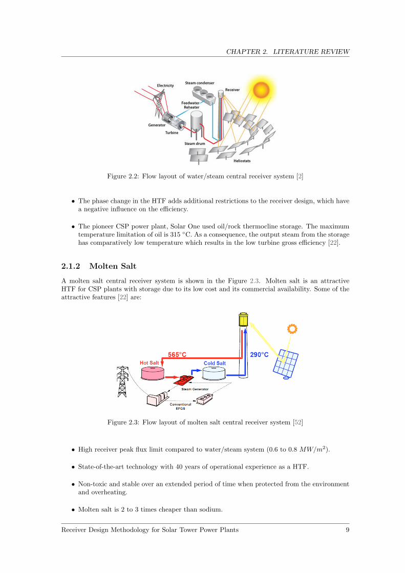
2.1.2 Molten Salt
A molten salt central receiver system is shown in the Figure 2.3. Molten salt is an attractiveHTF for CSP plants with storage due to its low cost and its commercial availability. Some of theattractive features [22] are:
Figure 2.3: Flow layout of molten salt central receiver system [52]
• High receiver peak flux limit compared to water/steam system (0.6 to 0.8 MW/m2).
• State-of-the-art technology with 40 years of operational experience as a HTF.
• Non-toxic and stable over an extended period of time when protected from the environmentand overheating.
• Molten salt is 2 to 3 times cheaper than sodium.
Receiver Design Methodology for Solar Tower Power Plants 9

CHAPTER 2. LITERATURE REVIEW
Figure 2.4: Flow layout of liquid sodium central receiver system [22]
2.1.3 Liquid Sodium
A liquid sodium central receiver system is shown in the Figure 2.4. Attributing to the fact thatliquid sodium has very good heat transfer properties, it has low thermal losses due to the reducedarea of the receiver. Mostly, sodium receivers are external type with already reduced losses, hencefurther loss reduction with cavity type receiver is not shown to be beneficial [22]. Compared tomolten salt, liquid sodium has very good heat transfer properties [22] as indicated below:
• High thermal conductivity results in operating the receiver with high incident solar flux (inexcess of 1.5 MW/m2).
• Sodium freezes at 100 ◦C which is two times lower when compared to molten salt.
• Sodium has a high boiling point (873 ◦C) [13] which allows it to operate in high-temperatureBrayton power cycles.
• Receiver size and thermal losses are reduced due to the higher operational flux resulting ina better receiver efficiency.
But, there are many limiting factors which act as a hindrance for sodium receiver to be commer-cially accomplished. Some of them [22] are stated below:
• The relatively high cost and low specific heat of sodium limit its usage as sensible heatstorage medium.
• Low volumetric heat capacity of sodium makes the storage tank large and costly.
• The main point to note is that the highly reactive nature of sodium and water has to beconsidered while designing and it adds a high risk.
2.1.4 Sodium/Salt Binary
Sodium/salt binary central receiver system is shown in the Figure 2.5. Sodium is used as areceiver fluid and molten salt is used as a storage fluid in sodium/salt binary system. It combinesthe attractive features of both fluids, but an additional heat transfer loop is needed for the systemto run, which adds complexity. The risk of sodium fire is reduced, because it is restricted withinthe concrete tower. However, the reaction between sodium and molten salt is not well-known.Current indications are that it would be strongly exothermic and release the gaseous product,which may lead to pressurisation problem [22].
10 Receiver Design Methodology for Solar Tower Power Plants

CHAPTER 2. LITERATURE REVIEW
Figure 2.5: Flow layout of sodium/salt binary central receiver system [22]
2.2 Design Criteria
This section summarises critical receiver design parameters.
2.2.1 Receiver Design Methodology
This section summarises the various receiver design methodologies that are available in the liter-ature. Figure 2.6 depicts the sketch of external and tubular receivers.
Figure 2.6: Tubular receivers: a) External receiver, b) Cavity receiver [10]
Falcone [1986]
Falcone [22] suggested the following steps for tubular receiver design:
1. Calculate the thermal rating of the receiver based on system level requirements like plantoutput, type of receiver fluid and storage media, nature of power cycle and solar multiple.
2. Select the flux limit based on working fluid and tube material of the receiver.
3. Calculate the required receiver absorber area for the given allowable flux limit.
4. Design the receiver geometry, taking into account thermal loss and the practical size of thereceiver. The minimum receiver size is largely a function of spillage considerations based onthe size of reflected heliostat image. The maximum practical size is limited by the height ofreceiver panels due to shipping constraints.
Receiver Design Methodology for Solar Tower Power Plants 11

CHAPTER 2. LITERATURE REVIEW
Zavoico [2001]
Zavoico [55] suggested the following steps for tubular receiver design:
1. Establish the allowable incident flux as a function of bulk salt temperature, allowable cumu-lative tube strains and corrosion rates at the salt film temperature.
2. Estimate the receiver size based on the maximum allowable flux.
3. Estimate the heat losses for various combinations of receiver height and diameter.
4. The aspect ratio should be selected for the maximum receiver efficiency and low cost.
Lata [2008]
Lata et al. [30] tried to optimize the receiver dimensions in order to increase the allowable peakflux of molten salt receiver from 0.85 MW/m2 to 1 MW/m2. Basically, this design methodologyis similar to others. In addition, the authors tried to optimise the following receiver dimensions.
1. Receiver size optimisation to minimise the thermal losses (Aspect ratio selection).
2. Selection of small tube diameter to maximise the receiver thermal efficiency and to preventfatigue-creep damage (Tube diameter selection).
3. Selection of thin tube wall to improve thermal efficiency (Tube wall thickness selection).
4. Minimise the pressure losses by optimising the number of panels and molten salt circuitrouteing (Number of panels and fluid path selection).
5. Selection of high nickel alloy material with excellent mechanical properties (Material selec-tion).
System Advisory Model (SAM)
The performance model of SAM uses the TRNSYS components developed at the University ofWisconsin [52]. The solar field optimisation algorithm is based on the DELSOL3 model developedat the Sandia national laboratory [52]. It is capable of operating in two modes. The first one cal-culates the performance of an existing system. The second one is an optimisation of system design.
In the optimisation process, the tower height and receiver sizes are iteratively evaluated to findout the minimum possible cost of electricity output. The optimisation process needs the initialguess defined by the user. They have developed an objective function for the minimisation of theenergy cost.
2.2.2 Allowable Peak Flux Limit
The typical range of flux limit for the receiver fluids is listed in the Table 2.1. It depends on thetube material and the required number of life cycles. Figure 2.7 shows the dependency of the peakallowable flux on the receiver life time for different HTF and materials [22]. With one cycle perday, 30 years receiver lifetime would lead to 11000 cycles. Also, one should take into account fortransients due to weather conditions. Alternatively, the allowable peak flux, qo can be calculatedbased on a model using the allowable thermal strain, thermal expansion and the poisson ratio ofthe material [32]. The average flux can be calculated by the peak-to-average flux ratio. Accordingto Stine and Harrigan [46], the peak-to-average flux ratio can be between 2 to 3.
12 Receiver Design Methodology for Solar Tower Power Plants

CHAPTER 2. LITERATURE REVIEW
Figure 2.7: Receiver peak flux value for different HTF and materials with respect to life cycles[22]
Name of the HTF Flux limit range Unit
Water/Steam 0.3 to 0.6 MW/m2
Molten Salt 0.6 to 1.2 MW/m2
Liquid Sodium 1.2 to 1.75 MW/m2
Table 2.1: Receiver flux limit for different HTF [22]
2.2.3 Receiver Sizing
Incident receiver thermal power should be estimated in order to size the receiver. Then, the al-lowable average flux should be determined based on the HTF and material (see section 2.2.2) tocalculate the absorber area required to handle the flux. Selection of the allowable peak flux has tobe done carefully to avoid thermal stress and fatigue-creep failure. Generally, one-half to one-thirdof the peak flux [46] is selected as an average flux. The receiver is sized for the average flux inorder to ensure that it will not fail.
For cavity receivers, the inner surfaces of the receiver are exposed to re-radiation because ofthe enclosed structure, which may lead to overheating. According to Falcone [22], the receiver sizefor cavity receivers is 25 percent larger than the external receiver for the same incident receiverthermal power. So, the average flux is selected accordingly for the cavity receivers in order toensure that it will not fail.
2.2.4 Receiver Aspect Ratio
According to Falcone [22], the receiver aspect ratio (height-to-diameter ratio) should be between 1to 2. It should be optimised based on the trade-off between thermal and spillage losses. Accordingto Zavoico [55], the receiver aspect ratio will be in the range of 1.2 to 1.5 and it should be selectedfor maximum receiver efficiency. For cavity receivers, it is usually in the range of 0.7 to 1 [22].Some additional design considerations from literature are:
• The shipping constraint of the sub-assembly of panel tubes and the maximum continuous
Receiver Design Methodology for Solar Tower Power Plants 13

CHAPTER 2. LITERATURE REVIEW
length of available seamless tubing limit the receiver height to 30m [22]. However, thereare some power plants which slightly cross this limit. Crescent Dunes Solar Energy Projectin US has the receiver height of 30.48 m [4] and the Atacama-1 project in Chile has beenplanned with a receiver height of 32 m [1].
• A taller height receiver is desirable so that the spillage is minimised [55].
• A larger diameter receiver is desirable to maximise the interior space available to place allthe receiver components, however large diameter will increase the thermal losses. So, spaceallocation design analysis should also be considered to optimise the aspect ratio [55].
2.2.5 Tube Diameter Selection
The receiver tube diameter can vary between 20 mm to 45 mm [30]. The tube material is generallystainless steel or Incoloy. The analysis by Lata [30] states the following:
• Small diameters increase the receiver efficiency due to the increased salt velocity and heattransfer coefficient. However, small diameters increase the manufacturing cost and the pres-sure drop. The pressure drop is directly proportional to the length of the salt circuit and tothe square of the salt velocity and it is inversely proportional to the tube diameter. There-fore, a trade-off between pressure drop and receiver efficiency should be done to optimisethe tube diameter.
• Thin tube walls increase the heat transfer rate due to the reduced conductive resistance inthe tubes. However, in practise, the wall thickness is limited to commercial values.
2.2.6 Fluid Flow Path Selection
Figure 2.8: Eight possible fluid flow configuration by Wagner [52]
The fluid flow path is chosen in such a way that it can distribute the local peak flux on the receiverevenly. The number of fluid flow paths has an influence on the pressure drop. Falcone [22] statesthat upward fluid flow is preferable so that the buoyancy force of the fluid does not counteractwith the pumping pressure. Molten salt has a high volumetric heat capacity, which results in lowvolume flow for a given power level [22]. Thus, for molten salt receivers, multi-pass flow is neededto get high velocities and high wall heat transfer coefficients. Consequently, it is difficult to realiseupward flow configurations in all panels. Hence, serpentine flow (up and down) is a reasonablealternative flow configuration. Wagner [52] developed a receiver model to analyse the behaviourof solar power plants and studied eight possible fluid flow configurations of the receiver, which are
14 Receiver Design Methodology for Solar Tower Power Plants

CHAPTER 2. LITERATURE REVIEW
depicted in the Figure 2.8. The following suggestions are given by Wagner to design an efficientreceiver:
• It is observed that the configuration with a single flow path has high pressure drop, whichincreases the parasitic pump power. Hence, two parallel flow paths in the receiver aresuggested in order to obtain better overall efficiency of the plant.
• In Northern hemisphere, the northern panels will receive high flux due to the sun positionduring peak hours. If cold fluid enters through the high flux northern panels, it will leadto high thermal losses. Thus, the south to north flow configuration gives high efficiency inthe northern hemisphere. However, in this configuration, the hot fluid from the south sidewill not be able to cool the high flux northern panels during peak hours. Consequently, thenorthern panels are exposed to high thermal stresses, which is not recommendable. Hence,in the Northern hemisphere, the north to south flow configuration with two parallel flowpath with or without a crossover is recommended.
Rodriguez-Sanchez [39] simulated the same eight flow configurations as Wagner to select the bestwith the aim of increasing the receiver availability and the global efficiency of the CRS plant. Sheobtained results similar to that of Wagner and proposed the north to south flow configurationwith one crossover in the middle as the best configuration based on the considerations of receiverthermal efficiency, distributed flux, tube temperature and thermal stress.
2.2.7 Tower Sizing
The tower height is mainly a function of the receiver thermal power of the plant [22]. The towerheight is also influenced by the type of solar field. Falcone [22] presented a graph (see Figure 3.4)which shows the range of tower height for a given receiver thermal power and the type of solarfield. The towers can be built of steel or concrete. Figure 2.9 shows both steel and concrete typetower. The tower investment cost increases with increasing height.
Figure 2.9: Solar tower for external and cavity receivers [23]
2.3 Cavity Specific Design Criteria
The following section consists of design criteria specific for cavity receivers. There is no specificdesign criteria needed for external receivers.
Receiver Design Methodology for Solar Tower Power Plants 15

CHAPTER 2. LITERATURE REVIEW
2.3.1 Cavity Receiver Geometry
The cavity receiver geometry is designed to reduce thermal losses by enclosing the absorber tubesinside a protecting cavity. The receiver aspect ratio acts as a primary design parameter for thecavity receiver geometry, which is shown in the Figure 3.4.1. It is usually in the range of 0.7 to 1[22]. The aspect ratio determines the width and height of the aperture opening and the radius ofthe cavity. All the piping and headers are placed inside the cavity, so there is some space neededon the top and bottom of the absorber tubes. This needs to be considered while designing thecavity receiver geometry. Generally, these headers are not exposed to direct irradiation and canbe covered by a lip to reduce heat losses. The design of the lip is explained in the subsection 2.3.3.Similar to active surfaces, the inactive surfaces are also heated up due to re-radiation and hence,careful selection of receiver allowable flux is necessary.
Figure 2.10: Cavity receiver geometry with four receiver panels [23]
2.3.2 Cavity Opening Angle
The cavity opening angle depends on the solar field arrangement. The cavity opening angle shouldbe similar to the covered angle of the radiation to the receiver from the solar field, so that thespillage loss will be reduced. Most commercial plants are designed with a cavity opening angleof 180◦ [23]. Lukas [23] calculated the receiver thermal efficiency with varying cavity openingangle. He observed that the receiver thermal efficiency increases with increasing cavity openingangle more than 180◦. Since increasing the cavity opening angle more than 180◦ decreases theaperture opening for a single cavity receiver, heat loss will be reduced. However, it is not possibleto distribute the heat flux uniformly for a high cavity opening angle. Therefore, it can't be appliedin real applications [23].
2.3.3 Lip Height (Aperture-to-Total Height Ratio)
The lip height is usually calculated by using the aperture-to-total height ratio. The differencebetween the total height to aperture height is known as lip height, which is shown in the Figure2.11. The lip which is placed above the aperture, is called upper lip, whereas the lip which is placed
16 Receiver Design Methodology for Solar Tower Power Plants

CHAPTER 2. LITERATURE REVIEW
Figure 2.11: Lip height of cavity receiver [33]
below the aperture, is called lower lip. Generally, the upper lip reduces the heat losses while thelower lip doesn't have much influence on the latter [29]. The value of aperture-to-total height ratioused by Lukas is 0.75 [23]. If the aperture-to-total height ratio is further increased, the spillageloss is increased. Hence, a trade-off should be done in order to optimise the aperture-to-totalheight ratio.
2.3.4 Cavity Inclination
The cavity inclination can vary from 0◦ to 90◦, which is depicted in the Figure 2.12. The convectiveheat loss of the cavity receiver depends on the wind speed, wind direction and cavity inclination.Flesch [25] conducted a cryogenic wind tunnel experiment and observed the influence of wind onthe convective loss for head-on and side-on wind direction. Cavity inclination reduces convectiveheat losses [18] [19]. However, wind speed increases convective heat losses particularly for inclinedcavities. From the analysis of cryogenic wind tunnel experiment, Flesch [25] observed that thecavities should be designed in such a way, that the wind flow is parallel to the aperture plane inorder to have a positive or at least non-negative influence of wind. Moreover, cavity inclination isrecommended in order to reduce the convection losses [25].
Figure 2.12: Cavity inclination angle [33]
2.4 Heat Transfer Model
This section covers heat loss models from literature for external convection, radiation and reflec-tion. Conduction loss to the back side of the receiver panel is small compared to other losses [46],so it is neglected in this study. An overview of various heat transfer models is summarised in thissection. It is divided into two subsections, external and cavity receivers.
Receiver Design Methodology for Solar Tower Power Plants 17

CHAPTER 2. LITERATURE REVIEW
2.4.1 External Receiver
In case of external receivers, the entire absorber area is exposed to the surroundings. Hence, thereare higher thermal losses from the receiver to the surroundings compared to cavity receivers [22].The main thermal losses are convection and radiation heat loss.
Convective Heat Loss
The heat transfer equations for the convection heat loss of cylindrical receivers are comparableto the correlations found in common heat transfer literature. However, the Nusselt correlationthat can be applied to large-scale receivers is an ambiguous field, in which a lot of research isbeing carried out [43] [15]. For cylindrical receivers, convective heat transfer is influenced by bothnatural and forced convection. Hence, mixed convection is usually considered [43]. In order tofind out which heat transfer is dominant, the Richardson number is used [48], which is explainedin the subsection 2.4.2.
According to literature [15] [43], heat transfer coefficient for mixed convection, hmix can be calcu-lated with the following correlation. According to Cengel [15], the value m lies between 3 and 4.The value close to 3 suits better for vertical surfaces and the larger values are suited for horizontalsurfaces. Siebers [43] studied this value and estimated the best-suited value of 3.2 for externalreceivers.
hmix = (hmnat + hmfor)1/m (2.1)
where
• hnat = Heat transfer coefficient due to natural convection, W/m2 K
• hfor = Heat transfer coefficient due to forced convection, W/m2 K
Natural Convection Loss
Natural convection loss occurs due to buoyancy effects and Nusselt correlations are given by manyauthors. The Nusselt correlation which can be applied for large-scale solar external receiver isgiven below:
Churchill and Chu [1975]: This correlation is used for the design of base-load nitrate saltcentral power plants by Abengoa [49]. This research is carried out in Sandia national lab in US[49]. All the fluid properties are calculated at the film temperature, Tf = Tamb+Ts
2 .
Nunat =
(0.825 +
0.387Ra1/6L(
1 + (0.492/Pr)9/16)8/27
)2
RaL < 1012 (2.2)
For laminar flows, the following correlation is slightly more accurate. It is observed that a transitionfrom laminar to turbulent boundary flow occurs when RaL exceeds 109. This correlation is validup to 109.
Nunat =
(0.68 +
0.67Ra1/4L(
1 + (0.492/Pr)9/16)4/9
)10−1 < RaL < 109 (2.3)
Rayleigh number, Ra is defined as the product of Grashof number and the Prandtl number andit is given in the form of equation below:
Ra = Gr · Pr (2.4)
The Grashof number, Gr can be calculated by the following equation:
Gr = g · β · (Ts,avg − Tamb) ·H3rec/νfluid (2.5)
where
18 Receiver Design Methodology for Solar Tower Power Plants

CHAPTER 2. LITERATURE REVIEW
• g = Acceleration due to gravity, m/s2
• β = Volumetric expansion coefficient, 1/K
• Ts,avg = Average surface temperature of the receiver, K
• Tamb = Ambient temperature, K
• Hrec = Height of the receiver, m
• νfluid = Kinematic viscosity, m2/s
The Prandtl number, Pr is defined as the ratio of viscous diffusion rate and thermal diffusion rate.It can be calculated by using the equation below:
Pr =µ/ρ
k/cpρ=cpµ
k(2.6)
where
• µ = Dynamic viscosity, kg/ms
• ρ = Density, kg/m3
• k = Thermal conductivity, W/mK
• cp = Specific heat, J/kgK
Siebers and Kraabel [1984] [43]: This correlation is widely used for the convective heat losscalculation of solar receivers [17]. The authors stated that there is nearly 40 percent uncertaintyin the equation [43]. All the fluid properties are calculated at the ambient temperature, Tamb.
Nunat = 0.098 ·Gr1/3 · (Ts/Tamb)−0.14 (2.7)
Forced Convection Loss
The forced convection loss occurs due to the influence of wind. Nusselt correlations which can beapplied to the large-scale solar external receiver are described below:
Churchill and Bernstein [1977] [15]: The following correlation is valid for Re · Pr > 0.2[15]. Christian and Clifford [17] stated that this correlation is valid for Reynold’s number up to4 × 105. Therefore, this correlation can't be used for high Reynold’s number due to high windspeeds [17]. All the fluid properties are calculated at the film temperature, Tf .
Nufor = 0.3 +0.62 ·Re1/2 · Pr1/3
[1 + (0.4/Pr)2/3]1/4
[1 +
(Re
282000
)5/8]4/5
(2.8)
Reynolds number, Re is defined as the ratio of inertial and the viscous forces. It can be calculatedusing the following equation:
Re =uwind ·Drec
νair(2.9)
where
• uwind = Wind velocity, m/s
• Drec = Diameter of the receiver, m
Receiver Design Methodology for Solar Tower Power Plants 19

CHAPTER 2. LITERATURE REVIEW
Reynolds Number Range Correlation
Ks/Drec = 0 (A smooth cylinder)
(1) All Re Nufor = 0.3 + 0.488 ·Re0.5 ·(
1 +(
Re282000
)0.625)0.8Ks/Drec = 75× 10−5
(2) Re ≤ 7.0× 10⁵ Use correlation (1)
(3) 7.0× 10⁵ < Re < 2.2× 10⁷ Nufor = 2.57× 10⁻³ ·Re0.98
(4) Re ≥ 2.2× 10⁷ Nufor = 0.0455 ·Re0.81
Ks/Drec = 300× 10−5
(5) Re ≤ 1.8× 10⁵ Use correlation (1)
(6) 1.8× 10⁵ < Re < 4× 10⁶ Nufor = 0.0135 ·Re0.89
(7) Re ≥ 4× 10⁶ Use correlation (4)
Ks/Drec = 900× 10−5
(8) Re ≤ 1× 10⁵ Use correlation (1)
(9) Re > 1× 10⁵ Use correlation (4)
Ks is the radius of the receiver tube, m
Table 2.2: Nusselt correlation for forced convection of external receivers [43]
Siebers and Kraabel [1984] [43]: This correlation is widely used for the convective heat losscalculation of solar receivers [17]. The correlations are shown in the Table 2.2. All the fluid prop-erties are calculated at the film temperature, Tf .
Cengel [2003] [15]: In this correlation, the fluid can be either gas or liquid but it is validbetween the Reynolds number range of 4×10⁴−4×10⁵. This correlation is used for the design ofbase-load nitrate salt central power plant by Abengoa [49]. This research is carried out in Sandianational lab in US [49].
Nufor = 0.027 ·Re0.805 · Pr1/3 (2.10)
Long-wave Radiation Heat Loss
The radiation heat loss, Qloss,rad is simple for external receivers and it can be calculated usingStefan-Boltzmann law. The external receiver is coated with the black coating to increase theabsorptivity. Generally, black pyromark is used to coat the receiver panels and housing [55].
Qloss,rad = σ · εeff ·Aproj · (T 4s,avg − T 4
amb) (2.11)
The effective emittance is given by the following equation [54]:
εeff =ε
ε+ (1− ε) · 2π(2.12)
where
• σ = Stefan-Boltzmann constant, 5.670 · 10−8W/m2K4
• εrec = Emissivity of the receiver
• Aproj = Projected area of the receiver, m2
20 Receiver Design Methodology for Solar Tower Power Plants

CHAPTER 2. LITERATURE REVIEW
• Ts,avg = Average surface temperature, K
• Tamb = Ambient temperature, K.
The average surface temperature of the receiver, Ts,avg can be calculated using mean radianttemperature. It can be given by the following equation:
Ts,avg =
(T 4s,hot + T 4
s,cold
2
)1/4
(2.13)
where
• Ts,hot = Hot surface temperature, K
• Ts,cold = Cold surface temperature, K
The calculation for surface temperature of the receiver is explained in the subsection 3.2.4.
Reflection Heat Loss
The part of the radiation which is reflected away from the receiver surface is called reflective heatloss. It can be calculated by using the absorptance of the receiver coating. The following equationgives the reflective heat loss, Qloss,ref from the receiver surface:
Qloss,ref = (1− αeff ) · Qth,rec (2.14)
With αeff = Effective absorptance due to the curvature of receiver tubes. The curvature of thetubes has to be taken into account while calculating the absorptance. The effective absorptance,αeff can be calculated by [54]:
αeff =α
α+ (1− α) · 2π(2.15)
2.4.2 Cavity Receiver
In this subsection, the heat transfer models specific for cavity receivers are discussed. In cavityreceivers, the absorber tubes are enclosed in a cavity to reduce the thermal losses. Similar toexternal receivers, the main thermal losses in cavity receivers are convection heat loss and radiationheat loss.
Convective Heat Loss
In order to find out which convective heat transfer is predominant, the Richardson number can beused [48]. With the help of this number, it is easy to find out what kind of convection mechanismhas to be included in the heat transfer model. The Richardson number, Ri is defined as the ratioof the Grashof number to the square of the Reynolds number.
Ri = Gr/Re2 (2.16)
• If the Richardson number is much greater than unity, natural convection dominates overforced convection.
• If it is much lower than unity, natural convection is negligible and forced convection domin-ates the heat transfer.
In order to have an idea about Richardson number, Teichel [48] plotted the Richardson numberwith respect to varying wind speed, which is shown in the Figure 2.13. From the Figure 2.13, onecan conclude that natural convection is dominant for wind velocities less than 5 m/s while forcedconvection dominates for wind velocities higher than 25 m/s.
Receiver Design Methodology for Solar Tower Power Plants 21

CHAPTER 2. LITERATURE REVIEW
Figure 2.13: Variation of Richardson number with respect to wind velocity for cavity receiver [48]
Generally, the maximum wind velocity will be nearly 20 m/s at the height of the receiver [48]and as a result, only natural convection or mixed convection can be expected in the large CRSreceivers. However, the wind velocity can exceed the previously stated value depends on the site.
However, the forced convection on large-scale cavity receivers has not been sufficiently studied.But, there are several studies on small scale cavity receivers [35] [47] and the heat losses due towind velocity and direction [33] [25] are also studied. Therefore, it is not well known whetherthese correlations can be applied to large central receivers of CSP towers.
Natural Convection Loss
Convection heat loss for the cavity receiver can be well explained with the two-zone model. Figure2.14 shows the stagnant zone and convective zone of the cavity receiver.
• The stagnant zone is the region, where the air is standing still and the temperature is closeto the wall temperature [25].
• The convection zone is the region, where the cold air enters through the aperture opening,gets heated up and leaves through the upper part of the aperture [25].
Increasing wind speed can shrink the stagnant zone [25]. This can be seen as a reason for the lowwind dependency of non-inclined cavities, as their stagnant zone is comparatively small.
Clausing(1983): In 1983, Clausing [19] published analytical and experimental modelling res-ults for test cavities in a cryogenic wind tunnel experiment conducted at the University of Illinois,Urbana-Champaign. Based on the results, he developed a natural convection heat transfer correl-ation. According to Clausing, the circulating flow inside the cavity is mainly due to the buoyancyeffects at boundary layers of the active surfaces [23]. However, it can be affected by the wind inflowand its direction. Clausing considered the wind velocity in the bulk flow velocity inside the cav-ity. Convection heat losses will not be greatly influenced by wind velocities lower than 8 m/s. Hedeveloped a correlation which allows calculating a heat transfer coefficient specific for each surface.
22 Receiver Design Methodology for Solar Tower Power Plants

CHAPTER 2. LITERATURE REVIEW
Figure 2.14: Two-zone model of the cavity receiver [25]
The correlation can be applied only if the heat transfer is dominated by internal resistances andwind effects don't have a large influence. This model is valid for Rayleigh numbers greater than1.6× 109 and the temperature ratio of wall to ambient being between 1 and 2.6. It is numericallyvalidated for no-wind and head-on wind conditions. According to Teichel [48], the temperatureratio of a typical receiver is between 1.8 and 3.4, so it is out of range for some conditions.
Clausing(1987): Clausing [20] updated his previous model by experimental investigation ofsmooth, isothermal cubic cavities with a variety of side facing apertures to predict the convectionloss for large-scale solar receivers. The large-scale receivers are modelled using the cryogenic windtunnel at the University of Illinois, Urbana Champaign. Using the results, Clausing came up witha correlation which is valid for large Rayleigh numbers and the large temperature ratio of wall toambient, hence it can be applied to large-scale solar receivers.
Unlike the previous model, this model was developed with only one heat transfer coefficient usingthe aperture area for the calculation of the convective losses of the entire cavity. This model isvalid for 3× 10⁷ ≤ Ra ≤ 3× 10¹⁰ and 1 ≤ Tw/Tamb ≤ 3. Higher Rayleigh numbers can occur forlarge-scale receivers, hence it might not be valid for all cases [48].
Siebers and Kraabel (1984): Siebers and Kraabel [43] came up with natural convection heattransfer correlation in 1984, which was based on the experimental work on cubical cavities byKraabel. They considered natural convection in large cavities to be similar to large vertical flatplates. They developed a Nusselt correlation for a simple cavity receiver with a validity range of105 ≤ Gr ≤ 1012. A correction factor is introduced in order to account for the aperture lips andthe tilt angle of the cavity. This model is validated with experimental measurements and it showsgood accordance with their results.
Forced Convection Loss
Forced convection has a significant influence on the convective heat transfer, but no reliable cor-relations are available to predict the forced convection heat transfer for cavity receivers. Theonly simple correlation that can be applied to cavity receivers is the correlation by Siebers andKraabel [43]. They used the forced convection correlation for vertical flat plate in order to account
Receiver Design Methodology for Solar Tower Power Plants 23

CHAPTER 2. LITERATURE REVIEW
for the wind effect. Their correlation was validated with the experimental data. The overall heattransfer coefficient for cavity receivers can be obtained by using the value of m as 1 in Equation 2.1
While this correlation was validated with a 4.5 MW test receiver at Sandia Lab, the forced con-vection values are mostly over-predicted. Thus, the model is conservative. The authors state thatthe equation is expected to have an uncertainty of more than 50 percent [43].
Long-wave Thermal Radiative Heat Loss
The thermal radiation from the active surfaces of a cavity receiver will directly or indirectly reachall the inactive surfaces and finally some part of the radiation will leave to ambient through theaperture opening. It is complex to determine the radiation heat losses accurately. Still, it can becalculated using view factors and there are two widely used methods to calculate radiation heatloss [48]. They are
• Radiosity method
• F-hat method
The view factors can be calculated using analytical or by ray tracing method. The analyticalmethod is limited to the specific cavity geometry with four receiver panels and for other geometries,ray tracing is used.
Reflection Heat Loss
Similar to long-wave thermal radiative heat loss, reflection heat loss can also be calculated withview factors using the same two methods as specified in subsection 2.4.2.
24 Receiver Design Methodology for Solar Tower Power Plants

Chapter 3
Design Methodology
In this chapter, the design approach for tubular receivers and the receiver design model for bothexternal and cavity receivers are discussed.
3.1 Design Approach
In this section, the steps required to design the receiver are summarised and shown in Figure 3.1.Furthermore, they are covered in detail in subsequent sections.
1. Calculate the incident receiver thermal power with the desired receiver output power andthe receiver thermal efficiency, which is assumed initially (see section 3.2.1).
2. Select receiver fluid and material.
3. Calculate the allowable peak flux limit on the receiver based on the type of HTF and thereceiver material. Subsequently, calculate the average allowable flux and size the receiverusing the average allowable flux (see section 3.2.3).
4. Design the receiver outer geometry using the aspect ratio (height-to-diameter ratio). It hasto be chosen considering the factor of minimal thermal and spillage loss of the receiver (seesection 3.3.1 for external receivers).
5. Fix the additional parameters like cavity opening angle, aperture-to-total height ratio andcavity inclination to design the receiver outer geometry for cavity receivers (see section 3.4.1).
6. Select the receiver tube diameter in such a way that the pressure loss is minimised and thereceiver efficiency is increased. A small diameter results in higher efficiency while in theother hand, it tends to increase the pressure losses (see section 3.3.2).
7. Select the tube wall thickness based on the pressure exerted by the fluid on the tube. Thinwall will lead to higher receiver efficiency, but it is limited by typical values of commercialtubes. Moreover, it should be able to hold the pressure and the tubes should not break (seesection 3.3.2).
8. Calculate the mass flow rate (see section 3.2.5) and fix the design fluid flow velocity. Then,the cross-sectional area required for the fluid flow is calculated using the mass flow rate, thevelocity and the density of the fluid. Once the cross-sectional area is known, the number oftubes and panels can be calculated by selecting the number of flow paths (see section 3.3.2).
9. Calculate the heat losses for the designed receiver and the actual efficiency is known. Hence,the previous steps are iteratively repeated until convergence is reached (see section 3.3.4 forexternal receivers and section 3.4.4 for cavity receivers).
Receiver Design Methodology for Solar Tower Power Plants 25

CHAPTER 3. DESIGN METHODOLOGY
10. Size the tower height with the receiver thermal power and the type of solar field (see section3.3.3 for external receivers and section 3.4.3 for cavity receivers).
Figure 3.1: Receiver design methodology for tubular receivers
26 Receiver Design Methodology for Solar Tower Power Plants

CHAPTER 3. DESIGN METHODOLOGY
3.2 General Receiver Design Model
This section describes the receiver design model which is common for both external and cavityreceivers.
3.2.1 Receiver Thermal Power
The first step is to calculate the incident receiver thermal power from the solar field. For thispurpose, the receiver output power is calculated and the receiver thermal efficiency is assumed.Then, the receiver thermal power, Qth,rec is calculated by
Qth,rec =Qth,pb
ηrec,guess· SM (3.1)
where
• Qth,pb = Thermal power required for power block, W
• ηrec,guess = Assumed receiver thermal efficiency
• SM = Solar multiple
3.2.2 Calculation of HTF Properties
The properties of HTF play a main role in the receiver design. Correlations for the properties ofsolar salt, hitec, hitec XL, therminol, liquid sodium and for some gases [12] are implemented. Theproperties for any other fluid can be given as an input to design the receiver with the particularfluid. The properties needed for the receiver model are density, specific heat capacity, dynamicviscosity and thermal conductivity. In this thesis, the focus is on molten salt receivers. Therefore,correlations to calculate solar salt properties are given in the Table 3.1.
Property Equation Units
Density ρ = 2090− (0.636 · Tmean,htf ) kg/m3
Specific heat capacity Cp = 1443 + 0.172 · Tmean,htf J/kgK
Dynamic viscosity µ = (22.714− (0.120 · Tmean,htf ) + (2.281× 10⁻⁴ · T 2mean,htf )− (1.474× 10⁻⁷ · T 3
mean,htf ))/103 Pa s
Thermal conductivity k = 0.443 + 1.9 · 10−4 · Tmean,htf W/m K
Tmean,htf is the mean fluid temperature, ◦C
Table 3.1: Properties of solar salt [55]
3.2.3 Receiver Sizing
Receiver sizing is done based on the allowable flux on the receiver. The allowable flux on thereceiver depends on the receiver material and the type of HTF. Generally, the allowable peak fluxfor molten salt receivers built with 316 Stainless steel material is 0.83 MW/m2 [22]. For receiversbuilt with Incoloy 800H, the allowable peak flux is 1 MW/m2 [32] [55]. So, these values are usedas the default values in the model.
The average allowable flux can be calculated with the peak-to-average flux ratio. Falcone useda specific value of 1.78 for external receivers and 2.65 for cavity receivers [22]. Because of thecavity enclosure, the inner surfaces of the receiver are exposed to re-radiation, which may lead tooverheating. Consequently, cavity receivers have high peak-to-average flux ratio. Therefore, theabsorber area is larger for the same receiver thermal power. The value used by Falcone is also in
Receiver Design Methodology for Solar Tower Power Plants 27
CHAPTER 3. DESIGN METHODOLOGY
accordance with the Gemasolar design flux [36] and therefore, it is used in this model. Using theaverage allowable flux, the area of the receiver, Arec can be calculated by
Arec =Qth,recqavg,flux
(3.2)
where
• qavg,flux = Allowable average flux of the receiver, W/m2
• Qth,rec = Incident receiver thermal power, W
3.2.4 Receiver Surface Temperature Calculation
It is assumed that the receiver has a uniform surface temperature. The heat transfer throughthe tube walls is calculated. The calculation takes into account conduction through the tube wallthickness and then convection to the receiver fluid. The surface temperature of the receiver iscalculated by calculating the resistance due to conduction and convection. The receiver surfacetemperature, Ts,avg can be obtained by:
Ts,avg = Qfluid · (Rcond +Rconv) + Thtf,avg (3.3)
With Thtf,avg = Average temperature of the receiver fluid, K. The resistance due to conductionthrough the tube walls, Rcond can be given by:
Rcond =ln(ro,tube/ri,tube)
2 · π ·Hrec · ktube · ntube(3.4)
where
• ro,tube = Radius of the receiver outer tube, m
• ri,tube = Radius of the receiver inner tube, m
• ntube = Total number of tubes in the receiver
The resistance due to internal convection between tube wall and the receiver fluid, Rconv can begiven by:
Rconv =1
hinner · π · ri,tube ·Hrec · ntube(3.5)
The heat transfer coefficient of internal convection between tube wall and the receiver fluid, hinnercan be given by the following equation:
hinner = Nu · kfluid/Lc (3.6)
With Lc = Characteristic length, which is the inner receiver tube diameter, di,tube. The Nusseltcorrelation by Dittus-Boelter [12] is used:
Nu = 0.023Re0.8Pr0.4 (3.7)
The above equation is valid for 0.7 < Pr < 120 and 104 < Re < 1.2× 10⁵. Using these equations,the surface temperature of the receiver is calculated.
28 Receiver Design Methodology for Solar Tower Power Plants

CHAPTER 3. DESIGN METHODOLOGY
3.2.5 Mass Flow Rate Calculation
The design mass flow rate of the receiver fluid is calculated with the absorbed receiver thermalpower. The minimum limitation of the mass flow rate to avoid any damage is given by theconstraint that the flow has to be turbulent. Thus, the Reynolds number has to be greater thanor equal to 4000 [39]. The mass flow rate, mhtf is calculated by:
mhtf =Qinc,rec · ηrec
cp,htf,avg · (Thtf,hot − Thtf,cold)(3.8)
where
• ηrec = Receiver thermal efficiency
• cp,htf,avg = Specific heat of the receiver fluid, J/kg K
• Thtf,hot = Outlet temperature of the hot receiver fluid, K
• Thtf,cold = Inlet temperature of the cold receiver fluid, K
3.2.6 Pressure Loss and Pump Power Calculation
The pressure drop in the receiver tubes, ∆Ptube is given by the following equation [15]. Thepressure loss due to the bends is not considered in this model.
∆Ptube = ρfluid · f ·Hrec
Dtube,inner·v2fluid
2(3.9)
With f = (0.790lnRe − 1.64)−2 for smooth tubes valid for 104 < Re < 106 and for rough tubes1√f
= −2.0 log(ε/D3.7 + 2.51
Re√f
).
where
• vfluid = Velocity of the receiver fluid, m/s
• ε/D = Relative roughness
The pressure drop for pumping the fluid up to the receiver, ∆Ptower is given by:
∆Ptower = ρfluid · g ·Htower (3.10)
With Htower = Height of the tower, m. The net presure drop across the receiver panels, ∆Pnet isgiven by:
∆Pnet = ∆Ptube ·npanelsnflowpath
+ ∆Ptower (3.11)
where
• npanels = Number of panels in the receiver
• nflowpath = Number of flow path in the receiver
The energy required to pump the receiver fluid through the receiver, Qpump is given by:
Qpump =∆Pnet · mhtf
ρfluid
ηpump(3.12)
With ηpump = Pump efficiency.
Receiver Design Methodology for Solar Tower Power Plants 29
CHAPTER 3. DESIGN METHODOLOGY
3.3 External Receiver Design Model
3.3.1 Geometry Design
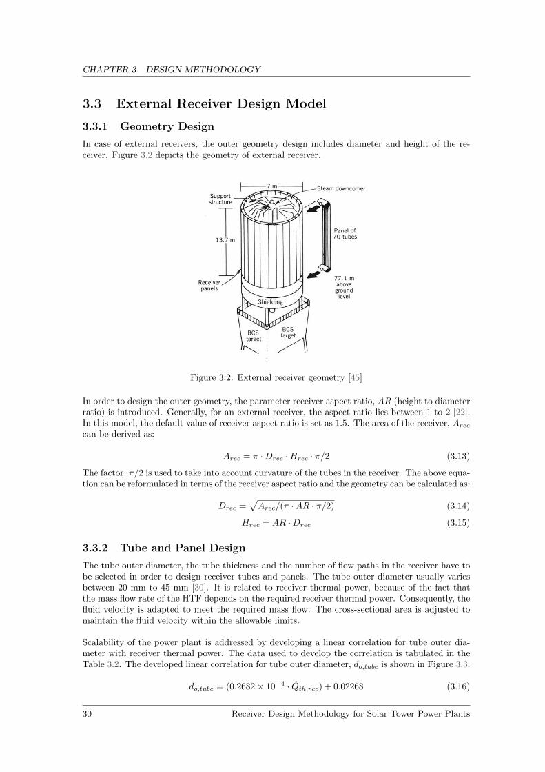
In case of external receivers, the outer geometry design includes diameter and height of the re-ceiver. Figure 3.2 depicts the geometry of external receiver.
Figure 3.2: External receiver geometry [45]
In order to design the outer geometry, the parameter receiver aspect ratio, AR (height to diameterratio) is introduced. Generally, for an external receiver, the aspect ratio lies between 1 to 2 [22].In this model, the default value of receiver aspect ratio is set as 1.5. The area of the receiver, Areccan be derived as:
Arec = π ·Drec ·Hrec · π/2 (3.13)
The factor, π/2 is used to take into account curvature of the tubes in the receiver. The above equa-tion can be reformulated in terms of the receiver aspect ratio and the geometry can be calculated as:
Drec =√Arec/(π ·AR · π/2) (3.14)
Hrec = AR ·Drec (3.15)
3.3.2 Tube and Panel Design
The tube outer diameter, the tube thickness and the number of flow paths in the receiver have tobe selected in order to design receiver tubes and panels. The tube outer diameter usually variesbetween 20 mm to 45 mm [30]. It is related to receiver thermal power, because of the fact thatthe mass flow rate of the HTF depends on the required receiver thermal power. Consequently, thefluid velocity is adapted to meet the required mass flow. The cross-sectional area is adjusted tomaintain the fluid velocity within the allowable limits.
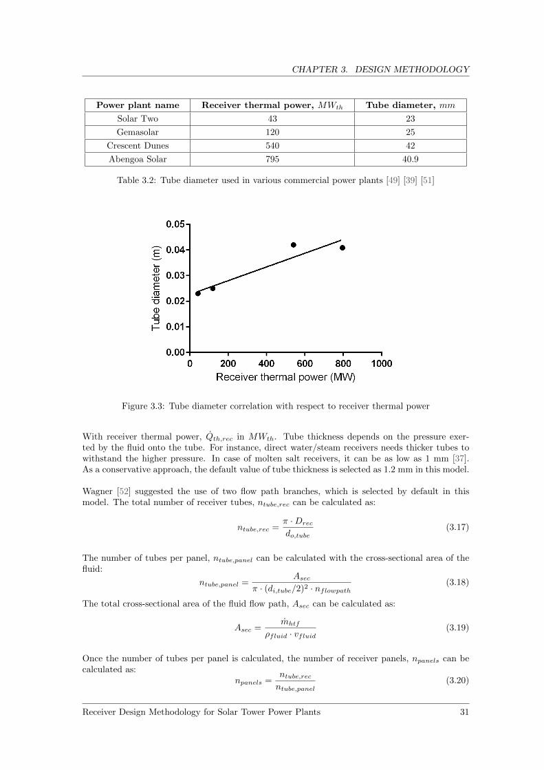
Scalability of the power plant is addressed by developing a linear correlation for tube outer dia-meter with receiver thermal power. The data used to develop the correlation is tabulated in theTable 3.2. The developed linear correlation for tube outer diameter, do,tube is shown in Figure 3.3:
do,tube = (0.2682× 10⁻⁴ · Qth,rec) + 0.02268 (3.16)
30 Receiver Design Methodology for Solar Tower Power Plants
CHAPTER 3. DESIGN METHODOLOGY
Power plant name Receiver thermal power, MWth Tube diameter, mm
Solar Two 43 23
Gemasolar 120 25
Crescent Dunes 540 42
Abengoa Solar 795 40.9
Table 3.2: Tube diameter used in various commercial power plants [49] [39] [51]
Figure 3.3: Tube diameter correlation with respect to receiver thermal power
With receiver thermal power, Qth,rec in MWth. Tube thickness depends on the pressure exer-ted by the fluid onto the tube. For instance, direct water/steam receivers needs thicker tubes towithstand the higher pressure. In case of molten salt receivers, it can be as low as 1 mm [37].As a conservative approach, the default value of tube thickness is selected as 1.2 mm in this model.
Wagner [52] suggested the use of two flow path branches, which is selected by default in thismodel. The total number of receiver tubes, ntube,rec can be calculated as:
ntube,rec =π ·Drec
do,tube(3.17)
The number of tubes per panel, ntube,panel can be calculated with the cross-sectional area of thefluid:
ntube,panel =Asec
π · (di,tube/2)2 · nflowpath(3.18)
The total cross-sectional area of the fluid flow path, Asec can be calculated as:
Asec =mhtf
ρfluid · vfluid(3.19)
Once the number of tubes per panel is calculated, the number of receiver panels, npanels can becalculated as:
npanels =ntube,recntube,panel
(3.20)
Receiver Design Methodology for Solar Tower Power Plants 31

CHAPTER 3. DESIGN METHODOLOGY
While designing, it should be taken care that the number of panels will also be even, if the numberof flow path is even. In this model, the number of panels are rounded to the next even number.
3.3.3 Tower Height Design
Figure 3.4: Variation of tower height with respect to receiver thermal power [22]
Currently, there is no reliable tower height model in the literature. Tower height is given as auser input in all the commercial design softwares. Falcone [22] has given a graph for tower heightwith respect to receiver thermal power, which is shown in Figure 3.4. Therefore, a correlationis developed by curve fitting with his values. However, the values are not in accordance withcommercial power plants, because the data is quite old. So, another correlation is developed usingstate-of-the-art commercial power plant and it is depicted in the Figure 3.5. The correlation forcalculating tower height for surround fields based on Falcone is given below:
Htower,min = 36.30075 + (0.3013896 · Qth,rec)− (0.1004369× 10⁻³ · Q2th,rec) (3.21)
Htower,max = 54.91579 + (0.3070526 · Qth,rec)− (0.1039793× 10⁻³ · Q2th,rec) (3.22)
Htower =Htower,min +Htower,max
2(3.23)
where
• Qth,rec = Receiver thermal power, MWth.
• Htower,min = Minimum tower height, m
• Htower,max = Maximum tower height, m
• Htower = Tower height, m
The following correlation is developed using state-of-the-art commercial power plant data:
Htower = 0.2552 · Qth,rec + 82.60 (3.24)
With Qth,rec = receiver thermal power in MWth.
32 Receiver Design Methodology for Solar Tower Power Plants

CHAPTER 3. DESIGN METHODOLOGY
Figure 3.5: Tower height correlation with respect to receiver thermal power for external receiver
3.3.4 Receiver Thermal Efficiency
The receiver thermal efficiency, ηrec is calculated by defining all thermal losses from the receiver.
ηrec = 1− Qloss,tot
Qth,rec(3.25)
With Qloss,tot = Total heat loss from the receiver in W . The heat loss model includes heat loss dueto reflection, external convection and radiation. The conduction to the back side of the receiverpanel is small compared to other losses and it is neglected [46].
Qloss,tot = Qloss,conv + Qloss,rad + Qloss,ref (3.26)
where
• Qloss,conv = Heat loss due to external convection, W
• Qloss,rad = Heat loss due to long-wave thermal radiation, W
• Qloss,ref = Heat loss due to reflection, W
Convection Heat Loss
The external receiver is usually approximated as a vertical cylinder. The following condition hasto be met to treat the receiver as vertical plate for the heat transfer correlations.
Drec
Hrec≥ 35
Gr14
(3.27)
The external convection heat loss equation is given below with the mixed convection heat transfercoefficient.
Qloss,conv = hmix ·Arec · (Ts,avg − Tamb) (3.28)
Mixed convection:
According to literature [43], most of the external solar receivers will undergo mixed convection. Itis calculated with equation 2.1.
Receiver Design Methodology for Solar Tower Power Plants 33

CHAPTER 3. DESIGN METHODOLOGY
Natural convection:
The heat transfer coefficient for natural convection, hnat can be calculated with the followingequation:
hnat = Nunat · kair/Hrec (3.29)
In this thesis, Siebers and Kraabel correlation is used for the heat transfer model because of itswide validity range. Furthermore, it was developed especially for large-scale solar receivers basedon experiments. Siebers and Kraabel correlation is given in the equation 2.7.
Forced convection:
The heat transfer coefficient for forced convection, hfor can be calculated with the following equa-tion:
hfor = Nufor · kair/Drec (3.30)
Similar to natural convection, Siebers and Kraabel correlation is also used for forced convectiondue to its wide validity range. Nusselt correlations for smooth and rough cylinders are shown inthe Table 2.2.
Long-wave Thermal Radiation Heat Loss
The model for radiative heat losses is explained in section 2.4.1.
Reflection Heat Loss
The model for reflective heat losses is explained in section 2.4.1.
3.4 Cavity Receiver Design Model
3.4.1 Geometry Design
Geometry design includes the radius of the cavity, height of the receiver, height of the absorber,lip height, width and height of the aperture, cavity opening angle and the cavity inclination angle.The aspect ratio usually ranges between 0.7 to 1 for cavity receivers [22]. The outer geometry ofcavity receiver is shown in the Figure 3.6.
Figure 3.6: Geometry of cavity receiver [23]
The following steps show how to calculate the width and height of the receiver aperture.
34 Receiver Design Methodology for Solar Tower Power Plants

CHAPTER 3. DESIGN METHODOLOGY
Once the absorber area is calculated with the allowable heat flux, width and height of the re-ceiver can be calculated by fixing the aspect ratio, AR and the cavity opening angle, θrec.
Aabs =θrecπ· π · rrec ·Habs ·
π
2(3.31)
where
• Aabs = Receiver absorber area, m2
• rrec = Radius of the receiver, m
• Habs = Height of the absorber, m
Figure 3.7: Internal angle geometry of cavity receiver [23]
The radius and height of the absorber can be calculated by rewriting the above equation in termsof the aspect ratio, which is shown below. In order to have an idea of receiver radius and itsinternal angle geometry, the cavity geometry is depicted in Figure 3.7.
rrec =
√Aabs
θrecπ · π2 ·AR
(3.32)
Habs = 2 ·AR · rrec (3.33)
The aperture width, Waper can be calculated from the following equation with the assumption ofreceiver width always being equal to aperture width or by fixing the aperture-to-total width ratio,(Waper
Wtot
)ratio
:
Waper = 2 · rrec · cos
(π − θrec
2
)·(Waper
Wtot
)ratio
(3.34)
In order to accommodate the receiver pipings and headers inside the cavity, extra space above theabsorber area is needed. After including the space, the overall height can be calculated with the
parameter gap-to-absorber height ratio,(Hgap
Habs
)ratio
:
Hrec = Habs ·[1 +
(Hgap
Habs
)ratio
](3.35)
The aperture height, Haper can be calculated with the aperture-to-total height ratio of the receiver,(Haper
Htot
)ratio
. It is chosen as 0.75 [48].
Haper =
(Haper
Htot
)ratio
·Hrec (3.36)
Receiver Design Methodology for Solar Tower Power Plants 35

CHAPTER 3. DESIGN METHODOLOGY
The lip height, Hlip can be calculated with total height of the receiver and the aperture. Only theupper lip is considered in the current model. The lip height of the receiver, Hlip can be calculatedby:
Hlip = Hrec −Haper (3.37)
3.4.2 Tube and Panel Design
The receiver tube and panel design is similar to external receivers except the calculation of numberof receiver tubes in the receiver. The number of receiver tubes can be calculated by
ntube,rec =π · rrec · θrecπ
do,tube(3.38)
3.4.3 Tower Height Design
Similar to external receivers, the tower height for cavity receivers is calculated by the correlationdeveloped by curve fitting Falcone values. The correlation is shown below:
Htower,min = 58.31818 + (0.4377023 · Qth,rec)− (0.0001802198 · Q2th,rec) (3.39)
Htower,max = 76.02273 + (0.4571479 · Qth,rec)− (0.0002080919 · Q2th,rec) (3.40)
Htower =Htower,min +Htower,max
2(3.41)
The correlation was updated by developing a new correlation using state-of-the-art commercialpower plants, which is shown in the Figure 3.8.
Htower = 0.6806 · Qth,rec + 106.6 (3.42)
Figure 3.8: Tower height correlation with respect to receiver thermal power for cavity receiver
36 Receiver Design Methodology for Solar Tower Power Plants

CHAPTER 3. DESIGN METHODOLOGY
3.4.4 Receiver Thermal Efficiency
The general procedure for calculation of receiver thermal efficiency is similar to that of externalreceivers. The heat losses which are calculated differently for cavity receivers are shown below.
Convection Heat Loss
It is assumed that the inactive surfaces and the air inside the cavity have higher temperatures dueto re-radiation.
Natural convection:
The following Nusselt correlation by Siebers and Kraabel [43] can be used to calculate the natural
Figure 3.9: Internal heat transfer area of the cavity receiver [43]
heat transfer coefficient:
Nu = 0.088Gr1/3(Ts,avgTamb
)0.18
105 ≤ Gr ≤ 1012 (3.43)
The correction factors are introduced to account for the effect of aperture lip and the cavityinclination. It is shown below:
hnc = hnc,0
(A1
A2
)(A3
A1
)n(3.44)
where
• n =(0.630.8
)→(θrec<30◦
θrec>30◦
)• Area A1, A2 and A3 are shown in the Figure 3.9.
The area used for heat transfer is the total interior surface of the cavity receiver, A1.
Forced convection:
The following Nusselt correlations by Siebers and Kraabel [43] can be used to calculate the forcedheat transfer coefficient:
Nu = 0.0287Re0.8Pr1/3 (3.45)
Receiver Design Methodology for Solar Tower Power Plants 37

CHAPTER 3. DESIGN METHODOLOGY
The area used for heat transfer is the aperture area of the cavity receiver.
Long-wave Thermal Radiation Heat Loss
The thermal radiation heat loss equation for the cavity receivers is given with the view factor:
Qloss,rad = σS · εeff · Fsurf−aper ·Asurf · (T 4s,avg − T 4
amb) (3.46)
In this thesis, a simple thermal radiation loss model is derived with the aperture opening area,assuming uniform temperature inside the cavity and using reciprocity and enclosure rules. If allthe surfaces inside the cavity are considered as a single surface, then the reciprocity rule for cavityreceivers is given by:
Faper−surf ·Aaper = Fsurf−aper ·Asurf (3.47)
With a view from the aperture to the cavity surface, the enclosure rule for cavity receivers is givenby:
N∑surf=1
Faper−surf = 1 (3.48)
Using these above equations, the view factor is replaced by specifying the aperture area:
Aaper = Fsurf−aper ·Asurf (3.49)
The following equation is used to calculate the radiation heat loss from the cavity receiver:
Qloss,rad = σS · εeff ·Aaper · (T 4s,avg − T 4
amb) (3.50)
This is assumed to be valid, if the average surface temperature of all surfaces inside the cavity isused. The effective emittance is given by the following equation [54]:
εeff =ε
ε+ (1− ε) · Aaper
Aproj
(3.51)
The cavity receiver is coated with black coating to increase the absorptivity. Generally, blackPyromark is used to coat the receiver panels [55].
Reflection Heat Loss
The reflection heat loss is reduced because of the enclosing cavity structure. The reflected radiationcan only leave through the aperture to reach the surroundings. The simple reflection loss equationis derived by assuming the receiver thermal power is uniformly distributed in the receiver. Similarto the thermal radiation approach, the following equation is used to calculate the reflected heatloss from the cavity receiver:
Qloss,ref = (1− αeff ) · Qth,recAproj
·Aaper (3.52)
where
• Aaper = Area of the aperture, m2
• Aproj = Projected area, m2 = θrecπ · π · rrec ·Habs
38 Receiver Design Methodology for Solar Tower Power Plants

Chapter 4
Implementation
This chapter discusses the implementation of the design method, its structure and the interfacefor external and cavity receivers to the in-house CRS plant design tool devISEcrs.
4.1 devISEcrs - A Design Tool
Figure 4.1: Modules of the devISEcrs design tool
There are six modules in the devISEcrs tool, which are shown in the Figure 4.1 and their func-tionality is discussed briefly below:
• The Design Point module calculates the design point conditions for which the power plantwill be designed.
• The Power Block module in the design tool computes the required thermal power, efficiency,mass flow rate and the gross-to-net conversion factor based on the design point calculations.
• A two tank molten salt storage is modelled in the Storage module, which computes thethermal power required for the storage, total mass and volume of the molten salt along withthe tank dimensions.
• Based on the storage calculations, the Solar Multiple module calculates the solar multiplewhich is used to design the solar field and the receiver. The solar multiple is used to definethe oversizing of the solar field, which is necessary to take into account the energy requiredfor storage.
• The Receiver module designs the receiver and computes the thermal losses. It is based onthe methodology derived in section 3.
Receiver Design Methodology for Solar Tower Power Plants 39

CHAPTER 4. IMPLEMENTATION
• The Solar Field module designs the solar field layout and calculates the optical losses of thesolar field.
4.2 Implementation Structure
As the devISEcrs tool is written in Python, the receiver module is also implemented in Python.The implementation is highly object-oriented. The code documentation is done using the doxygenstyle. The implementation structure of the receiver design method and the main functions areshown in the Figure 4.2.
Figure 4.2: Class inheritance structure of the receiver module in devISEcrs
The receiver module includes the design method for both types of receivers. As they share somecommon functionality, the External Receiver class and the Cavity Receiver class inherit from amore general Receiver class. The sub-division of the design methodology as described in section3 is implemented using functions.
Due to this structure, it is possible to use the receiver module for the design of the entire re-ceiver or the distinct investigations on specific aspects. Additionally, it is possible to manuallyoverwrite almost all default values used in the implementation.
40 Receiver Design Methodology for Solar Tower Power Plants
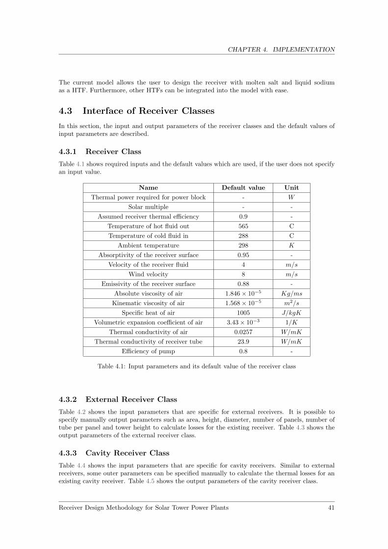
CHAPTER 4. IMPLEMENTATION
The current model allows the user to design the receiver with molten salt and liquid sodiumas a HTF. Furthermore, other HTFs can be integrated into the model with ease.
4.3 Interface of Receiver Classes
In this section, the input and output parameters of the receiver classes and the default values ofinput parameters are described.
4.3.1 Receiver Class
Table 4.1 shows required inputs and the default values which are used, if the user does not specifyan input value.
Name Default value Unit
Thermal power required for power block - W
Solar multiple - -
Assumed receiver thermal efficiency 0.9 -
Temperature of hot fluid out 565 C
Temperature of cold fluid in 288 C
Ambient temperature 298 K
Absorptivity of the receiver surface 0.95 -
Velocity of the receiver fluid 4 m/s
Wind velocity 8 m/s
Emissivity of the receiver surface 0.88 -
Absolute viscosity of air 1.846× 10⁻⁵ Kg/ms
Kinematic viscosity of air 1.568× 10⁻⁵ m2/s
Specific heat of air 1005 J/kgK
Volumetric expansion coefficient of air 3.43× 10⁻³ 1/K
Thermal conductivity of air 0.0257 W/mK
Thermal conductivity of receiver tube 23.9 W/mK
Efficiency of pump 0.8 -
Table 4.1: Input parameters and its default value of the receiver class
4.3.2 External Receiver Class
Table 4.2 shows the input parameters that are specific for external receivers. It is possible tospecify manually output parameters such as area, height, diameter, number of panels, number oftube per panel and tower height to calculate losses for the existing receiver. Table 4.3 shows theoutput parameters of the external receiver class.
4.3.3 Cavity Receiver Class
Table 4.4 shows the input parameters that are specific for cavity receivers. Similar to externalreceivers, some outer parameters can be specified manually to calculate the thermal losses for anexisting cavity receiver. Table 4.5 shows the output parameters of the cavity receiver class.
Receiver Design Methodology for Solar Tower Power Plants 41

CHAPTER 4. IMPLEMENTATION
Name Default value Unit
Heat transfer fluid Molten salt -
Receiver aspect ratio 1.5 -
Outer diameter of receiver tube Diameter correlation m
Thickness of receiver tube 0.0012 m
Number of flow path 2 -
Tower height Tower correlation m
Table 4.2: Input parameters and its default value of the external receiver class
Name Unit
Area of the receiver m2
Height of the receiver m
Diameter of the receiver m
Outer diameter of receiver tube m
Thickness of receiver tube m
Number of panels -
Number of tubes per panel -
Tower height m
Mass flow rate of the fluid kg/s
Minimum allowable mass flow rate kg/s
Incident receiver thermal power W
Table 4.3: Output parameters of the external receiver class
Name Default value Unit
Heat transfer fluid Molten salt -
Receiver aspect ratio 1 -
Cavity opening angle 180 degrees
Aperture to total height ratio 0.75 -
Aperture to total width ratio 1 -
Outer diameter of receiver tube Diameter correlation m
Thickness of receiver tube 0.0012 m
Number of flow path 2 -
Cavity inclination angle 0 degrees
Tower height Tower correlation m
Tower Orientation 180 degrees
Table 4.4: Input parameters and its default value of the cavity receiver class
42 Receiver Design Methodology for Solar Tower Power Plants

CHAPTER 4. IMPLEMENTATION
Name Unit
Area of the receiver m2
Total height of the receiver m
Diameter of the receiver m
Lip height m
Outer diameter of receiver tube m
Thickness of receiver tube m
Number of panels -
Number of tubes per panel -
Cavity opening angle degrees
Cavity inclination angle degrees
Tower height m
Mass flow rate of the fluid kg/s
Minimum allowable mass flow rate kg/s
Incident receiver thermal power W
Receiver normal vector -
Table 4.5: Output parameters of the cavity receiver class
Receiver Design Methodology for Solar Tower Power Plants 43

Chapter 5
Validation and Results
This chapter discusses the validation of the design method and the further results obtained usingthis model.
5.1 Receiver Design Validation
The receiver design methodology is validated using selected reference plants. The reference plantsare chosen in such a way that they are commercially well established and the plant data is availablein the literature. Then, a new receiver is designed for the reference case specifications using thedeveloped model and is compared against the reference plant to check the validity of the developeddesign method. This validation procedure is applied to external and cavity receivers.
5.1.1 External Receiver
The external receiver model is only validated with molten salt as HTF. Though other HTFs canbe used, the validation is limited to molten salt receiver in this thesis. Three solar power plantsof different sizes are used as reference cases. These are the 10 MW Solar Two power plant inCalifornia, the 20 MW Gemasolar power plant in Spain and the 110 MW Crescent Dunes powerplant in Nevada. All three are using the molten nitrate salt receiver technology.
Solar Two Power Plant
The Solar Two power plant is a 10 MW CRS plant with 3 hours of storage located in California,USA [51]. It was the first power plant developed with molten salt storage technology in 1996 [51]and it was demolished in 2009. A 43 MWth external nitrate salt receiver was constructed to meetthe demand of net electric power [51]. The plant location and characteristics are tabulated inTable 5.1.
Using the plant location and specifications, a new receiver is designed with the developed designmethod. The receiver is designed for the desired receiver thermal power. The resulting receiverdesign is compared with the actual Solar Two plant values.
Table 5.2 shows the results of devISEcrs model and the values of Solar Two power plant. Oncomparing receiver absorber area, it has a deviation of nearly 7 percent from the reference plantvalue, which is due to the deviation in allowable average design flux on the receiver. Solar Twopower plant used an average solar flux value of 430 KW/m2 and 465 KW/m2 is used in this model.The receiver diameter and height will be affected by the deviation of absorber area. Furthermore,the selection of receiver aspect ratio differs.
44 Receiver Design Methodology for Solar Tower Power Plants
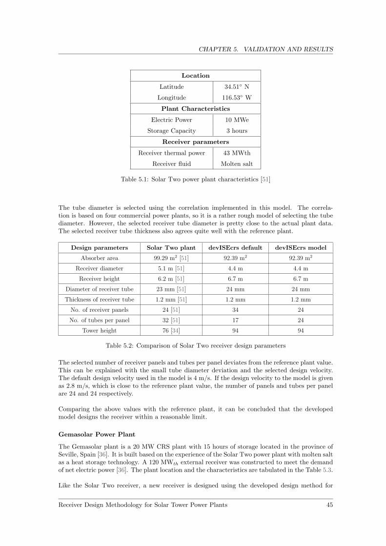
CHAPTER 5. VALIDATION AND RESULTS
Location
Latitude 34.51◦ N
Longitude 116.53◦ W
Plant Characteristics
Electric Power 10 MWe
Storage Capacity 3 hours
Receiver parameters
Receiver thermal power 43 MWth
Receiver fluid Molten salt
Table 5.1: Solar Two power plant characteristics [51]
The tube diameter is selected using the correlation implemented in this model. The correla-tion is based on four commercial power plants, so it is a rather rough model of selecting the tubediameter. However, the selected receiver tube diameter is pretty close to the actual plant data.The selected receiver tube thickness also agrees quite well with the reference plant.
Design parameters Solar Two plant devISEcrs default devISEcrs model
Absorber area 99.29 m2 [51] 92.39 m2 92.39 m2
Receiver diameter 5.1 m [51] 4.4 m 4.4 m
Receiver height 6.2 m [51] 6.7 m 6.7 m
Diameter of receiver tube 23 mm [51] 24 mm 24 mm
Thickness of receiver tube 1.2 mm [51] 1.2 mm 1.2 mm
No. of receiver panels 24 [51] 34 24
No. of tubes per panel 32 [51] 17 24
Tower height 76 [34] 94 94
Table 5.2: Comparison of Solar Two receiver design parameters
The selected number of receiver panels and tubes per panel deviates from the reference plant value.This can be explained with the small tube diameter deviation and the selected design velocity.The default design velocity used in the model is 4 m/s. If the design velocity to the model is givenas 2.8 m/s, which is close to the reference plant value, the number of panels and tubes per panelare 24 and 24 respectively.
Comparing the above values with the reference plant, it can be concluded that the developedmodel designs the receiver within a reasonable limit.
Gemasolar Power Plant
The Gemasolar plant is a 20 MW CRS plant with 15 hours of storage located in the province ofSeville, Spain [36]. It is built based on the experience of the Solar Two power plant with molten saltas a heat storage technology. A 120 MWth external receiver was constructed to meet the demandof net electric power [36]. The plant location and the characteristics are tabulated in the Table 5.3.
Like the Solar Two receiver, a new receiver is designed using the developed design method for
Receiver Design Methodology for Solar Tower Power Plants 45

CHAPTER 5. VALIDATION AND RESULTS
the respective plant location and specifications. The receiver is designed for the desired receiverthermal power and the resulting receiver design is compared with the actual Gemasolar plantvalues.
Location
Latitude 37.33◦ N
Longitude 5.19◦ W
Plant Characteristics
Electric Power 19.9 MWe
Storage Capacity 15 hours
Receiver parameters
Receiver thermal power 120 MWth
Receiver fluid Molten salt
Table 5.3: Gemasolar power plant characteristics [36]
The actual and designed receiver design parameters are listed in the Table 5.4. The designed ab-sorber area is smaller when compared to the actual plant value. This is because of the differencein allowable average design flux on the receiver. In the Gemasolar power plant, the allowableaverage design flux used is 445 KW/m2, whereas this model uses 465 KW/m2. The receiverdiameter and height are influenced by the absorber area, which therefore also deviates to someextent. Moreover, the aspect ratio used is also different between the actual plant and the model.Gemasolar is using an aspect ratio of 1.3 and the model is using 1.5 as a default value.
Design parameters Gemasolar plant devISEcrs model devISEcrs model
Absorber area 269.6 m2 [36] 256.64 m2 256.64 m2
Receiver diameter 8.1 m [36] 7.2 m 7.2 m
Receiver height 10.6 m [36] 11.3 m 11.3 m
Diameter of receiver tube 25 mm [7] 26 mm 26 mm
Thickness of receiver tube 1.65 mm [37] 1.2 mm 1.2 mm
No. of receiver panels 16 [37] 22 16
No. of tubes per panel 64 [37] 40 56
Tower height 140 m [21] 114 m 114 m
Table 5.4: Comparison of Gemasolar receiver design parameters
The designed tube diameter is close to the actual tube diameter, because the correlation of thetube diameter is developed based on state-of-the-art commercial plants. There is a deviation intube thickness, which is kept constant for molten salt receivers in the model. The tube thicknesshas to be selected based on the pressure exerted by the fluid, so that the tube can withstand thepressure. Mostly, pressure is not crucial for molten salt receivers. In case of water/steam receivers,care should be taken to design the tube thickness according to the high operating pressure in thereceiver.
Though the tube diameter is close to the actual value, the number of panels and tubes per panelare different due to the selected design velocity. If the design velocity is given as 2.8 m/s, which
46 Receiver Design Methodology for Solar Tower Power Plants

CHAPTER 5. VALIDATION AND RESULTS
is close to the reference plant value, the number of panels and the tubes per panel are 16 and 56respectively. The small difference in tubes per panel from the reference plant can be explainedwith the small absorber area and receiver diameter. Tower height model is rather rough and there-fore there is some deviation in the tower height. However, the developed design method designs areasonable receiver that accords to that of commercial plants.
Crescent Dunes Power Plant
The Crescent Dunes power plant is a 110 MW solar tower power plant with 10 hours of storagelocated in Tonopah, Nevada, USA [37]. It is a large scale power plant with molten salt techno-logy and is developed by SolarReserve. A 540 MWth external molten salt receiver is used for therequired net electric power [37]. There is no detailed literature for the receiver thermal powerused in Crescent Dunes power plant. Therefore, the receiver thermal power is calculated with thedesign mass flow rate of the plant (1280 kg/s), which is found in the literature [37]. Rodriguez [37]mentioned that the Crescent Dunes plant generates four times more electric power than Gemasolarwhich is in accordance with the calculated receiver thermal power. The plant location and thespecifications are tabulated in the Table 5.5.
Location
Latitude 38.14◦ N
Longitude 117.22◦ W
Plant Characteristics
Electric Power 110 MWe
Storage Capacity 10 hours
Receiver parameters
Receiver thermal power 540 MWth
Receiver fluid Molten salt
Table 5.5: Crescent Dunes power plant characteristics [37]
Using the plant location and specifications, the developed design method designs a new receiver.Similar to the previous reference cases, the receiver is designed for the desired receiver thermalpower. The resulting receiver design is compared with the actual reference plant values.
The actual and designed receiver design parameters are listed in the Table 5.6. The actual receiverthermal power is calculated with the design mass flow rate and it might not be accurate. Hence,there will be a deviation in absorber area, which in turn influences the receiver diameter andheight. However, the deviation of the designed absorber area from the real value is less than 5 %.
The tube diameter has a deviation of 5 mm from the reference plant. However, the tube dia-meter can be selected over a wide range for the same receiver thermal power. The number ofpanels and the tubes per panel will be changed according to the tube diameter and fluid velocity.For the design velocity of 4 m/s, the number of panels and the tubes per panel are 16 and 83respectively. The result is close to the actual plant data. As explained in the previous section, aconstant tube wall thickness is used in this model.
Comparing the designed receiver parameters to the actual plant data, the results correspondto the commercial power plants.
Receiver Design Methodology for Solar Tower Power Plants 47
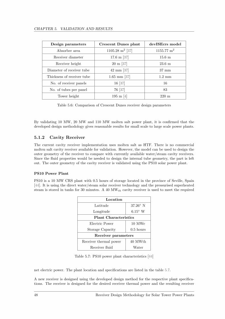
CHAPTER 5. VALIDATION AND RESULTS
Design parameters Crescent Dunes plant devISEcrs model
Absorber area 1105.28 m2 [37] 1155.77 m2
Receiver diameter 17.6 m [37] 15.6 m
Receiver height 20 m [37] 23.6 m
Diameter of receiver tube 42 mm [37] 37 mm
Thickness of receiver tube 1.65 mm [37] 1.2 mm
No. of receiver panels 16 [37] 16
No. of tubes per panel 76 [37] 83
Tower height 195 m [4] 220 m
Table 5.6: Comparison of Crescent Dunes receiver design parameters
By validating 10 MW, 20 MW and 110 MW molten salt power plant, it is confirmed that thedeveloped design methodology gives reasonable results for small scale to large scale power plants.
5.1.2 Cavity Receiver
The current cavity receiver implementation uses molten salt as HTF. There is no commercialmolten salt cavity receiver available for validation. However, the model can be used to design theouter geometry of the receiver to compare with currently available water/steam cavity receivers.Since the fluid properties would be needed to design the internal tube geometry, the part is leftout. The outer geometry of the cavity receiver is validated using the PS10 solar power plant.
PS10 Power Plant
PS10 is a 10 MW CRS plant with 0.5 hours of storage located in the province of Seville, Spain[44]. It is using the direct water/steam solar receiver technology and the pressurised superheatedsteam is stored in tanks for 30 minutes. A 40 MWth cavity receiver is used to meet the required
Location
Latitude 37.26◦ N
Longitude 6.15◦ W
Plant Characteristics
Electric Power 10 MWe
Storage Capacity 0.5 hours
Receiver parameters
Receiver thermal power 40 MWth
Receiver fluid Water
Table 5.7: PS10 power plant characteristics [44]
net electric power. The plant location and specifications are listed in the table 5.7.
A new receiver is designed using the developed design method for the respective plant specifica-tions. The receiver is designed for the desired receiver thermal power and the resulting receiver
48 Receiver Design Methodology for Solar Tower Power Plants
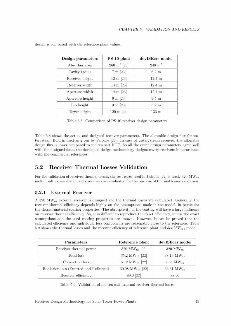
CHAPTER 5. VALIDATION AND RESULTS
design is compared with the reference plant values.
Design parameters PS 10 plant devISEcrs model
Absorber area 260 m2 [23] 248 m2
Cavity radius 7 m [23] 6.2 m
Receiver height 12 m [23] 12.7 m
Receiver width 14 m [23] 12.4 m
Aperture width 14 m [23] 12.4 m
Aperture height 9 m [23] 9.5 m
Lip height 3 m [23] 3.2 m
Tower height 120 m [44] 133 m
Table 5.8: Comparison of PS 10 receiver design parameters
Table 5.8 shows the actual and designed receiver parameters. The allowable design flux for wa-ter/steam fluid is used as given by Falcone [22]. In case of water/steam receiver, the allowabledesign flux is lower compared to molten salt HTF. As all the outer design parameters agree wellwith the designed data, the developed design methodology designs cavity receivers in accordancewith the commercial references.
5.2 Receiver Thermal Losses Validation
For the validation of receiver thermal losses, the test cases used in Falcone [22] is used. 320 MWth
molten salt external and cavity receivers are evaluated for the purpose of thermal losses validation.
5.2.1 External Receiver
A 320 MWth external receiver is designed and the thermal losses are calculated. Generally, thereceiver thermal efficiency depends highly on the assumptions made in the model, in particularthe chosen material coating properties. The absorptivity of the coating will have a large influenceon receiver thermal efficiency. So, it is difficult to reproduce the exact efficiency, unless the exactassumptions and the used coating properties are known. However, it can be proved that thecalculated efficiency and individual loss components are reasonably close to the reference. Table5.9 shows the thermal losses and the receiver efficiency of reference plant and devISEcrs model.
Parameters Reference plant devISEcrs model
Receiver thermal power 320 MWth [22] 320 MWth
Total loss 35.2 MWth [22] 38.19 MWth
Convection loss 5.12 MWth [22] 4.88 MWth
Radiation loss (Emitted and Reflected) 30.08 MWth [22] 33.31 MWth
Receiver efficiency 89.0 [22] 88.06
Table 5.9: Validation of molten salt external receiver thermal losses
Receiver Design Methodology for Solar Tower Power Plants 49

CHAPTER 5. VALIDATION AND RESULTS
Figure 5.1: Total and individual loss component comparison for external receiver
The absorptance used in the model is 0.95. The calculated receiver efficiency agrees reasonablywell with the reference plant receiver efficiency. Figure 5.1 shows the comparison of convectionand radiation losses contribution for designed and actual external receiver. In this model, 0 m/s isused as a design wind velocity [37]. The radiation loss includes the emitted and reflected radiation.The estimated convective loss is quite close to the reference value and there is some deviation inradiation losses. This can be explained with the deviation in coating properties. However, thecalculated values are in the reasonable range. Hence, the developed loss model is assumed to bevalid for molten salt external receivers.
5.2.2 Cavity Receiver
Similar to the external receiver, a 320 MWth molten salt cavity receiver is designed and thethermal losses are calculated. Table 5.10 shows the thermal losses and the receiver efficiency ofboth reference plant and devISEcrs model.
Parameters Reference plant devISEcrs model
Receiver thermal power 320 MWth [22] 320 MWth
Total loss 29.44 MWth [22] 23.42 MWth
Convection loss 10.24 MWth [22] 8.37 MWth
Radiation loss (Emitted and Reflected) 19.2 MWth [22] 15.05 MWth
Receiver efficiency 90.8 [22] 92.68
Table 5.10: Validation of molten salt cavity receiver thermal losses
50 Receiver Design Methodology for Solar Tower Power Plants

CHAPTER 5. VALIDATION AND RESULTS
Figure 5.2: Total and individual loss component comparison for cavity receiver
The absorptance used in the model is 0.95. The calculated receiver efficiency is 92 percent whichis close to the actual efficiency of 91 percent. Figure 5.2 shows the comparison of convection andradiation losses contribution for designed and actual cavity receiver. Similar to external receiver,0 m/s is used as a design wind velocity for cavity receiver also. The radiation loss consists ofboth emitted and reflected radiation. The deviation of radiation losses can be explained with theassumptions made in this model and the deviation in coating properties. However, the modelis estimating thermal losses in the reasonable range and therefore, it is assumed to be valid formolten salt cavity receiver.
5.3 Effect of Spillage Loss on Heliostat Size
Spillage loss has to be within a reasonable limit. After careful analysis using the devISEcrs tool, itis found that the spillage loss is largely influenced by the heliostat size, particularly for small-scalepower plants.
Due to astigmatism, the reflected beam size on the receiver increases with increasing heliostatsize. In case of large-scale power plants, the receiver size is big enough to accept the large reflec-ted beam produced by large heliostats. However, care should be taken while determining heliostatsize for small scale receivers in order to restrict spillage loss to a reasonable limit.
Figure 5.3 shows the external receiver spillage loss for different power plant sizes with respectto heliostat size. The effect of increased spillage is most significant for small-scale power plants.General trade-off between high spillage losses and high heliostat field costs which arise for using avery high number of heliostats.
It is shown in the Figure 5.3 that small size power plants are more prone to high spillage losseswith respect to heliostat size. So, it is essential to select an appropriate heliostat size in order torestrict the spillage loss to a reasonable limit.
Receiver Design Methodology for Solar Tower Power Plants 51

CHAPTER 5. VALIDATION AND RESULTS
Figure 5.3: External receiver spillage loss of different power plant sizes with respect to heliostatsize
Figure 5.4: Cavity receiver spillage loss of different power plant sizes with respect to heliostat size
Figure 5.4 depicts the cavity receiver spillage loss for different power plant sizes with respectto heliostat size. The spillage loss is lower for cavities than external receivers because of largeaperture size for the same receiver thermal power. Therefore, the size of the power plant selectedfor the cavity receivers is restricted to the 10 MW power plant. Similar to external receivers,cavity receivers are also more prone to spillage loss with respect to heliostat size for small-scalepower plants. Hence, it is suggested to use a heliostat size that corresponds to the receiver sizefor small-scale power plants.
52 Receiver Design Methodology for Solar Tower Power Plants

Chapter 6
Conclusion and Future Work
6.1 Conclusion
A methodology was developed to design molten salt tubular receivers by using and adapting ex-isting design criteria available in the literature. It was implemented in Python and embedded inthe Fraunhofer ISE tool, devISEcrs.
The developed receiver will be able to design/calculate:
• Outer receiver geometry
• Internal tube geometry
• Loss estimation
The developed design methodology was validated by comparing to four different commercialpower plants. The resulting receiver designs are in accordance with the commercial power plants.Moreover, the scalability of the design method is considered and the model is able to design smallto large-scale power plants.
Spillage losses depending on heliostat and receiver size were studied.
6.2 Future Work
Possible future improvements may include:
• Development of a method to calculate the allowable peak flux with the given receiver fluidand material.
• Inclusion of the aiming point strategy to estimate the flux on the receiver surface.
• Implementation of a more detailed pressure loss calculation considering pressure loss due tobends and headers.
• Development of a method to calculate cavity inclination angle for cavity receivers.
• Replacement of the tower height model with a more sophisticated one.
Receiver Design Methodology for Solar Tower Power Plants 53

Bibliography
[1] Atacama solar tower project, Chile. http://www.nrel.gov/csp/solarpaces/project_
detail.cfm/projectID=3275. Accessed: 2016-06-28. 14
[2] Concentrated solar power plant. https://www.eeremultimedia.energy.gov/solar/
/graphics/concentrating_solar_power_tower_plant_illustration. Accessed: 2016-06-22. vivi, 9
[3] Concentrated solar power plant with subsystems. http://reneweconomy.com.au/2013/
how-it-works-solar-power-towers-with-integrated-storage-78892. Accessed: 2016-08-05. vivi, 3
[4] Crescent dunes solar energy project, USA. http://www.nrel.gov/csp/solarpaces/
project_detail.cfm/projectID=60. Accessed: 2016-06-28. 14, 48
[5] CSP power plant types. http://www.solar-tower.org.uk/quick-start.php. Accessed:2016-06-21. vivi, 4
[6] Gemasolar power plant in spain. http://www.torresolenergy.com/EPORTAL_IMGS/
GENERAL/SENERV2/IMG2-cw4e41253840d81/gemasolar-plant-june2011-2b.jpg. Ac-cessed: 2016-06-21. vivi, 5
[7] Gemasolar tube diameter data. http://www.finetubes.co.uk/case-studies/
gemasolar-the-worlds-first-commercial-solar-power-plant-which-can-generate/.Accessed: 2016-07-18. 46
[8] Solar irradiation types. http://desktop.arcgis.com/en/arcmap/10.3/tools/
spatial-analyst-toolbox/modeling-solar-radiation.htm. Accessed: 2016-06-21.vivi, 1
[9] Solar receiver. http://www.csp-world.com/news/20130402/00805/
molten-salt-receiver-crescent-dunes-csp-plant-complete. Accessed: 2016-06-22. vivi, 6
[10] Solar tubular receivers. https://www.osapublishing.org/oe/fulltext.cfm?uri=
oe-24-14-A985. Accessed: 2016-08-05. vivi, 11
[11] Omar Behar, Abdallah Khellaf, and Kamal Mohammedi. A review of studies on centralreceiver solar thermal power plants. Renewable and sustainable energy reviews, 23:12–39,2013. 2, 3
[12] H Benoit, L Spreafico, D Gauthier, and G Flamant. Review of heat transfer fluids in tube-receivers used in concentrating solar thermal systems: Properties and heat transfer coeffi-cients. Renewable and Sustainable Energy Reviews, 55:298–315, 2016. 27, 28
[13] Nicholas Boerema, Graham Morrison, Robert Taylor, and Gary Rosengarten. Liquid sodiumversus hitec as a heat transfer fluid in solar thermal central receiver systems. Solar Energy,86(9):2293–2305, 2012. 10
54 Receiver Design Methodology for Solar Tower Power Plants

BIBLIOGRAPHY
[14] Ch. Breyer and G. Knies. Global energy supply potential of concentrating solar power. InProceedings of SolarPACES 2009, Berlin, September 15 18, 2009. 2
[15] Yunus Cengel. Heat transfer a practical approach, mcgraw-hill korea. 2003. 18, 19, 20, 29
[16] ZS Chang, X Li, C Xu, C Chang, and ZF Wang. The design and numerical study of a 2mwhmolten salt thermocline tank. Energy Procedia, 69:779–789, 2015. 4
[17] Joshua M Christian and Clifford K Ho. Cfd simulation and heat loss analysis of the solar twopower tower receiver. In ASME 2012 6th International Conference on Energy Sustainabilitycollocated with the ASME 2012 10th International Conference on Fuel Cell Science, Engin-eering and Technology, pages 227–235. American Society of Mechanical Engineers, 2012. 19,20
[18] AM Clausing. An analysis of convective losses from cavity solar central receivers. SolarEnergy, 27(4):295–300, 1981. 17
[19] AM Clausing. Convective losses from cavity solar receiverscomparisons between analyticalpredictions and experimental results. Journal of Solar Energy Engineering, 105(1):29–33,1983. 17, 22
[20] AM Clausing, JM Waldvogel, and LD Lister. Natural convection from isothermal cubicalcavities with a variety of side-facing apertures. Journal of heat transfer, 109(2):407–412,1987. 23
[21] Francisco J Collado and Jesus Guallar. A review of optimized design layouts for solar powertower plants with campo code. Renewable and Sustainable Energy Reviews, 20:142–154, 2013.46
[22] Patricia Kuntz Falcone. A handbook for solar central receiver design. Technical report, SandiaNational Labs., Livermore, CA (USA), 1986. vivi, vivi, vivi, vivi, viiiviii, 8, 9, 10, 11, 12, 13,14, 15, 16, 18, 27, 30, 32, 34, 49, 50
[23] Lukas Feierabend. Thermal Model Development and Simulation of Cavity-Type Solar CentralReceiver Systems. 2010. vivi, vivi, vivi, vivi, 6, 15, 16, 17, 22, 34, 35, 49
[24] Austin Fleming, Charles Folsom, Heng Ban, and Zhiwen Ma. A general method to analyzethe thermal performance of multi-cavity concentrating solar power receivers. Solar Energy,2015. 6
[25] Robert Flesch, Hannes Stadler, Ralf Uhlig, and Bernhard Hoffschmidt. On the influence ofwind on cavity receivers for solar power towers: An experimental analysis. Applied ThermalEngineering, 87:724–735, 2015. vivi, 17, 22, 23
[26] Charles W Forsberg. Developments in molten salt and liquid-salt-cooled reactors. In Pro-ceedings of the ICAPP. Citeseer, 2006. 4
[27] D Yogi Goswami and Frank Kreith. Energy conversion. CRC press, 2007. 6, 8
[28] D Kearney, U Herrmann, P Nava, B Kelly, R Mahoney, J Pacheco, R Cable, N Potrovitza,D Blake, and H Price. Assessment of a molten salt heat transfer fluid in a parabolic troughsolar field. Journal of solar energy engineering, 125(2):170–176, 2003. 4
[29] JS Kraabel. An experimental investigation of the natural convection from a side-facing cubicalcavity. In Proceedings of the ASME JSME Thermal Engineering Joint Conference, Honolulu,HI, Mar, pages 20–24, 1983. 17
[30] Jesus M Lata and Monica Rodriguez, Manuel Alvarez de Lara. High flux central receivers ofmolten salts for the new generation of commercial stand-alone solar power plants. Journal ofSolar Energy Engineering, 130(2):021002, 2008. 6, 12, 14, 30
Receiver Design Methodology for Solar Tower Power Plants 55

BIBLIOGRAPHY
[31] Zhirong Liao and Amir Faghri. Thermal analysis of a heat pipe solar central receiver forconcentrated solar power tower. Applied Thermal Engineering, 102:952–960, 2016. 6
[32] Zhirong Liao, Xin Li, Chao Xu, Chun Chang, and Zhifeng Wang. Allowable flux density ona solar central receiver. Renewable Energy, 62:747–753, 2014. 12, 27
[33] Robert Y Ma. Wind effects on convective heat loss from a cavity receiver for a parabolicconcentrating solar collector. Sandia National Laboratories, 1993. vivi, vivi, 17, 22
[34] James E Pacheco, RW Bradshaw, DB Dawson, W De la Rosa, R Gilbert, SH Goods, MJ Hale,P Jacobs, SA Jones, GJ Kolb, et al. Final test and evaluation results from the solar twoproject. Report No. SAND2002-0120, Sandia National Laboratories, Albuquerque, NM, 2002.45
[35] M Prakash, SB Kedare, and JK Nayak. Investigations on heat losses from a solar cavityreceiver. Solar Energy, 83(2):157–170, 2009. 22
[36] S Relloso and E Garcıa. Tower technology cost reduction approach after gemasolar experience.Energy Procedia, 69:1660–1666, 2015. viiiviii, 28, 45, 46
[37] Rodriguez-Sanchez. On the design of solar external receivers. viiiviii, 31, 46, 47, 48, 50
[38] MR Rodriguez-Sanchez, A Sanchez-Gonzalez, C Marugan-Cruz, and D Santana. New designsof molten-salt tubular-receiver for solar power tower. Energy Procedia, 49:504–513, 2014. 6,7
[39] MR Rodriguez-Sanchez, A Sanchez-Gonzalez, C Marugan-Cruz, and D Santana. Flow pat-terns of external solar receivers. Solar Energy, 122:940–953, 2015. viiiviii, 15, 29, 31
[40] Marcelino Sanchez and Manuel Romero. Methodology for generation of heliostat field layout incentral receiver systems based on yearly normalized energy surfaces. Solar Energy, 80(7):861–874, 2006. 5
[41] MRI Sarker, Manabendra Saha, Md Sazan Rahman, and RA Beg. Recirculating metallicparticles for the efficiency enhancement of concentrated solar receivers. Renewable Energy,96:850–862, 2016. 6
[42] FMF Siala and ME Elayeb. Mathematical formulation of a graphical method for a no-blockingheliostat field layout. Renewable energy, 23(1):77–92, 2001. 5
[43] Dennis L Siebers and John S Kraabel. Estimating convective energy losses from solar centralreceivers. Technical report, Sandia National Labs., Livermore, CA (USA), 1984. vivi, viiiviii,6, 18, 19, 20, 23, 24, 33, 37
[44] Solucar. 10 mw solar thermal power plant for southern spain. Technical report, Ciemat, DLR,2006. viiiviii, 48, 49
[45] WB Stine. Power from the sun, published online by william b. stine and michael geyer, 2001.vivi, 1, 5, 6, 30
[46] William B Stine and Raymond W Harrigan. Solar energy fundamentals and design. 1985.12, 13, 17, 33
[47] T Taumoefolau, Sawat Paitoonsurikarn, Graham Hughes, and Keith Lovegrove. Experimentalinvestigation of natural convection heat loss from a model solar concentrator cavity receiver.Journal of Solar Energy Engineering, 126(2):801–807, 2004. 22
[48] Soenke Holger Teichel. Modeling and Calculation of Heat Transfer Relationship for Concen-trated Solar Power Receivers. 2011. vivi, 18, 21, 22, 23, 24, 35
56 Receiver Design Methodology for Solar Tower Power Plants

BIBLIOGRAPHY
[49] Drake Tilley, Bruce Kelly, and Frank Burkholder. Baseload nitrate salt central receiver powerplant design final report. Technical report, Abengoa Solar LLC, 2014. viiiviii, 18, 20, 31
[50] F Trieb et al. Global concentrating solar power potentials, 2010. vivi, 2
[51] Craig E Tyner et al. Solar two: A molten salt power tower demonstration. viiiviii, viiiviii,31, 44, 45
[52] Michael J Wagner. Simulation and predictive performance modeling of utility-scale centralreceiver system power plants. University of Wisconsin -Madison, 2008. vivi, vivi, vivi, 8, 9,12, 14, 31
[53] Min Wei, Yilin Fan, Lingai Luo, and Gilles Flamant. Design and optimization of baffled fluiddistributor for realizing target flow distribution in a tubular solar receiver. Energy, 2016. 6
[54] C-J Winter, Rudolf L Sizmann, and Lorin L Vant-Hull. Solar power plants: fundamentals,technology, systems, economics. Springer Science & Business Media, 2012. 20, 21, 38
[55] Al exis B Zavoico. Solar power tower design basis document. Technical report, SandiaNational Labs., 2001. viiiviii, 12, 13, 14, 20, 27, 38
Receiver Design Methodology for Solar Tower Power Plants 57