The Effect of Stolen Goods Markets on Crime: Evidence from a Quasi Natural Experiment

Rocco D’Este

No 1040 (revised)

WARWICK ECONOMIC RESEARCH PAPERS

DEPARTMENT OF ECONOMICS

The Effect of Stolen Goods Markets on Crime:Evidence from a Quasi Natural Experiment

Rocco d’Este∗†(University of Warwick)

May 22, 2014

Abstract

This paper investigates the effect of stolen goods markets on crime. We focus on pawnshops,a business that have long been suspected of illicit trade. The analysis of a unique panel datasetof 2176 US counties from 1997 - 2010 uncovers an elasticity of pawnshops to theft crimes of0.8 to 1.4. We then exploit the raise in gold price as a quasi - natural experiment, where theintensity of the treatment is given by the predetermined concentration of pawnshops in thecounty. A one standard deviation increase in pawnshops’ initial allocation raises the effect ofgold price on burglaries by 0.05 to 0.10 standard deviation. No effect is ever detected on anyother type of crime.

“If he’s coming in my store with a VCR, I’m not asking him where he got it. It’s the police’s jobto find out if it’s stolen, not mine. You don’t ask where things come from. If you don’t take those,the guy down the street will” (Glover and Larubbia, 1996)

1 Introduction

Theft crimes produce a substantial harm to society. In 2010, United States have experienced 1theft every 40.5 seconds, with an estimated total of 9.5 million crimes that caused an economic lossfor the victims of almost $16 billions (FBI, 2010).1 In 85% of the cases something different fromcash was stolen, strongly suggesting that burglars need a market where to convert stolen items into∗Special thanks for the support to Robert Akerlof, Mirko Draca, Rocco Macchiavello and Chris Woodruff. I

am indebted for the insightful discussions and useful comments to Sascha Becker, Dan Bernhardt, Clément deChaisemartin, Joseph Doyle, Justin McCrary, Magne Mogstad, Fabian Waldinger, Kimberley Scharf and all theparticipants of the CWIP (Warwick), ISC, PEUK and IAAE. I gratefully acknowledge the financial support from theEconomic and Social Research Council (ESRC) and the International Association of Applied Econometrics (IAAE).All errors and omissions remained are my own responsibility.†r.d-este@warwick.ac.uk1Personal calculation from the author, obtained summing up data on larceny, robbery, burglary and motor and

vehicle theft from the FBI reports for the year 2010.

1

profits. In particular, the local availability of stolen goods markets might affect criminals’ behaviorthrough two different channels: 1) reducing theft - related transaction costs and hence loweringburglars’ probability of arrest 2) increasing the price for the stolen property and - consequently -raising the expected benefits deriving from criminal activity. Nevertheless, despite the understand-ing of the link between demand and supply of crime seems to be of critical importance to reducethe proliferation of theft crimes, a systematic empirical investigation of the effect of stolen goodsmarkets on criminal behavior is missing.2 Two main obstacles hinder this type of analysis. First,markets for stolen properties are hardly identifiable. Secondly, these are not randomly assigned togeographic locations.

This paper investigates the effect of stolen goods markets on crime through the lens of pawnshops,a widespread legal business that have long been suspected of illicit trade. While the proponentsof these business, led by the National Pawnbrokers Association, stigmatize the frequency of thisphenomenon, public opinion, newspapers and criminologists point the finger against this “modernthief’s automatic cash machine” (Glover and Larubbia, 1996).

Despite the different standpoints, obtaining evidence on the effect of potential stolen goodsmarkets on the supply of crime is complicated by a number of reasons. Pawnshops mainly servethe credit needs of low income people. Hence, the endogenous sorting of pawnshops in communitieswith a large presence of potential customers biases upward ordinary least squares (OLS) estimates,given that these communities usually experience an higher level of crime. Further biases are causedby omitted variables that correlates with both the presence of pawnshops and crime, or by thepossibility that the endogenous sorting of pawnshops is a direct response of the expected level ofcrime in the community (reverse causality bias).

We address these issues in several ways. In the first part of the paper, the empirical strategy relieson the properties of a unique panel dataset constructed for the analysis: 2176 counties in 50 states,almost 70% of the US total, from 1997 to 2010. The structure of the panel allows for the inclusionof county fixed effect, that control for unobserved time invariant heterogeneity across counties.The baseline empirical analysis focuses on the effect of the within county variation in the numberof pawnshops on the number of reported theft crimes. Year fixed effects and states linear trends

2Different studies have analyzed a wide set of crime’s potential determinants. Among these we find: the effectof police and incarceration (Levitt 1997, Di Tella and Schargrodsky 2004, Klick and Tabarrok 2005, Levitt 1996,Levitt 1998, Helland and Tabarrok 2007, Drago, Galbiati and Vertova 2009, Lee and McCrary 2009, Draca, Machinand Witt 2011), conditions in prisons (Katz, Levitt and Shustorovich 2003), parole and bail institutions (Kuziemko2007), education (Western, Kling and Weiman 2001, Lochner and Moretti 2004), social interactions and peer effects(Case and Katz 1991, Glaeser, Sacerdote and Scheinkman 1996, Gaviria and Raphael 2001, Kling, Ludwig and Katz2005, Jacob and Lefgren 2003, Bayer, Hjalmarsson and Pozen 2009), family circumstances (Glaeser and Sacerdote1999, Donohue and Levitt 2001). Economists have also focused on the the effect of criminal histories on labor marketoutcomes (Grogger 1995, Kling 2006), the impact of unemployment and wages on crime (Grogger 1998, RaphaelandWinter- Ebmer 2001), the strategic interplay between violent and property crime (Silverman 2004), the optimallaw enforcement (Polinsky and Shavell 2000, Eeckhout, Persico and Todd 2009) the immigration status (Bianchi,Buonanno and Pinotti 2012) and the impact of violent movies and pornography on violent crimes (Dahl and DellaVigna 2009 and Bhuller, Havnes, Leuven and Mogstad 2011).

2

control for nationwide and state specific confounding shocks. Moreover, the analysis includes a richset of county, time varying, socioeconomic controls such as: income per capita, percentage of peoplebelow the poverty line, unemployment, the number of social security recipients, the average monthlypayment per subsidy, the number of commercial banks and saving institutions, the number of swornpolice officers and civilian employees, the population density and the racial/ethnic composition inthe county. Finally, to control for changes in drug penetration and risky behavior, we add dataon arrests for sale and possession of drugs (opium/cocaine, marijuana, synthetic drugs and otherdangerous non narcotics) and gambling (bookmaking horse and sports, numbers and lotteries andall other illegal gambling). The clear attempt is to shut down possible endogeneity concerns due tothe omission of county specific time varying unobservables.

Results are startling. Ordinary least squares estimates show a strong effect of pawnshops onlyon two specific theft crimes: larceny and burglary, with an elasticity of 1.4 and 0.8. These findingsare robust to extensive robustness checks, the clustering of standard errors at different levels, thesensitivity to outliers, weighting the regression by a measure of the quality of the informationavailable to the researcher, using different functional forms and excluding from the sample countieswith big population.

Moreover, implicit falsification tests on other crimes - that should not be directly affected by thepresence of these businesses - disprove the possibility that pawnshops might influence crime throughdifferent channels other than the potential demand for stolen goods. In particular, the availabilityof data on motor - vehicle thefts gives the possibility of unambiguously testing the hypothesis of thepaper. This particular theft crime is totally insensitive to the presence of pawnshops in the county,plausibly because motor and vehicles are never accepted in pawnshops’ transactions. Furthermore,no effect is detected on any other crime.

The effect on larcenies and burglaries is more acute in densely populated counties, where -plausibly - the anonymity of the environment amplifies the likelihood of the pawnshop being aconvenient destination for stolen items. In less densely populated areas instead, pawnshops mightbe far from the crime scene, crime is generally less frequent and residents are more willing to defendthe interests of the members of their communities. This might discourage thieves to use this channelto get rid of stolen items.

We further extend the analysis in the attempt to detect geographical spillover effects on crime.We do so by constructing other two different measures of pawnshops’ concentration 1) in borderingcounties 2) and at the state level. Interestingly, results show that within county changes in larceniesand burglaries are significantly affected from the variation of the number of pawnshops in the samecounty but also in the same state. These results partly confirm the findings obtained from severalburglars’ interviews (Sutton, 2010). In fact, knowing that the probability of arrest increases whilestolen property is in possession, burglars prefer to commit thefts at a maximum distance of half anhour by car from the predetermined resale point (Sutton, 2010). On the other hand, we also find

3

evidence that burglars might take the risk of traveling far from the crime scene, plausibly to avoidsuspects about the origin of the item or to outdistance the good from the place where it was stolen.

Despite the use of panel data techniques, the lack of random assignment of pawnshops to countiesposes two different threats to the identification of a causal parameter. First of all, results mightdriven by the omission of time variant unobservables both related to within county changes in thenumber of pawnshops and theft crimes. But, what magnitude should have the bias to completelyinvalidate our findings? The Altonji et al. (2005) method of assessing selection on unobservablesusing selection on observables is pursued in this context. The rule of thumb outlined in Nunn andWantchekon (2012) is that any ratio above 1 is acceptable. In our case the Altonjii ratio is above10 for theft crimes, finally suggesting that there is little concern that selection on unobservables isthe main driver of our results.

A second econometric concern is related to the bias arising from the reverse causality betweenpawnshops and larcenies/burglaries. Despite the interesting implication related to the positivesorting of pawnshops in counties with an high level of theft crimes, (conditional on all the covari-ates included in the dataset), we totally overcome this issue in the last section of the paper, byintroducing in the analysis the price of gold.

Gold has always been the major determinant of pawnbrokers’ profit function, roughly repre-senting 80 percent of the value of all pledges (Bos et al, 2012). Pawnbrokers’ demand for goldmaterializes through the request of jewelry. But, what makes jewelry and - in particular - goldso profitable for pawnbrokers’ activities? A big part of the pawnbrokers’ profits comes from theprocess of melting down the gold received by their clients through the “refinement” process. In fact,90% of the times pawnbrokers sell their jewelry to a company that is known as a ‘refiner.’ A refinerwill take all of the rings, necklaces, bracelets and other items and melt them. Truly professionaloutfits will then begin to remove impurities from the metals until they get something close to puregold. Hence, stolen jewelries might disappear forever from the second - hand market when aretransformed into a bar of precious metal.

This persistent demand for jewelry and gold in particular might influence criminal behavior. Infact, as in any other type of economic activity, the exact knowledge of the demand for stolen goodsmight affect the type of items that are actually stolen. The underlying hypothesis of the paper isthat the shift in the resale value of gold, exogenously determined by changes in the macroeconomicconditions, while potentially increasing burglars’ expected benefits of committing a theft uniformlyin all counties, might cause relatively more theft crimes in counties with an higher predeterminedconcentration of markets interested in acquiring gold. In practice, we further address the endogene-ity of pawnshops to crime exploiting the exogenous rise in the price of gold as a quasi - naturalexperiment, where the intensity of the treatment is given by the concentration of pawnshops in thecounty fixed to the first year of the sample.

Again, results strongly support our hypothesis. A one standard deviation increase in the initial

4

concentration of pawnshops in the county increases the effect of the rise of gold price on burglariesby 0.05 to 0.10 standard deviation. Conversely, the effect on larceny, that usually includes theftsof bicycles, motor vehicle parts and accessories, shoplifting, pocket-picking, or the stealing of anyproperty or article that is not taken by force, is noisy and not precisely estimated. As in the firstpart of the paper, no effect is detected on motor and vehicle thefts and on all other crimes. As afurther falsification test, we repeat the same exercise including the interaction between the initialconcentration of pawnshops and the price of copper. Reassuringly, we do not detect any positiveeffect on burglaries. In fact, objects containing copper, while being heavily targeted by criminals,are usually not accepted in pawnshops’ transactions.

This paper has the power to inform policy. A closer monitoring of pawnshops from local author-ities, (as well as of other potential markets for crime not considered in this paper), in fact seemsto be warranted. This improved monitoring could plausibly reduce the illegal demand for stolengoods and, consequently, the number of theft crimes in pawnshops’ surrounding area.

To conclude, we believe that the main and most relevant contribution of this paper is a firststep towards a systematic empirical investigation of the link between demand and supply of crime,an extremely important issue never properly explored in the existing literature on the determinantsof crime.

This paper proceeds as follows. Section 2 presents some suggestive evidence related to thelink between pawnshops and theft crimes. Section 3 presents the data and lays down the initialeconometric framework, reporting the different results, various robustness checks and heterogeneityin the results. Section 4 introduces the role of gold in the quasi natural experiment, outlines theresearch design and presents the results. Section 5 concludes the paper.

2 Pawnshops As a Market Place for Stolen Goods: Suggestive

Evidence

Pawnshops, payday loans and check cashing outlets are all businesses that provide credit to“unbanked” clients at a very high interest rates.3 Nevertheless, within all these activities, pawnbro-kers offer a unique service: the supply of instant cash to their clients, only through the exchangeof personal property’s items. The standard procedure begins with the assessment of the monetaryvalue of the item brought by the client. If the client agrees with the offer received, she can eitherdirectly sell the item to the pawnbroker or she can ask for a loan, using the pledge as a collateral.

3U.S. households purchased more than $40 billion in high-cost short-term loans using the “fringe banking sector”in 2007, Fellowes and Mabanta (2008). Even if there is no official and reliable estimate of the total number of clients,industry reports suggest that 34 million adults demanded the services of these companies. The sector consists ofseveral types of high-cost lenders, but two comprise the dominant portion: payday lenders and pawnshops. In 2007pawnshops made 42 million transactions for an overall value of 2.5 billion dollars. The maximum interest rate setby pawnbrokers and payday lenders is generally regulated at the state level. For a complete review of pawnshops’operating system see Shackman and Tenney (2006).

5

Usually, the offer ranges from 30 to 75 per cent of the market value of the pledge, with the averageloan value being 100$ for a two months period. The pawnbroker holds the personal item in custodyuntil the maturity date of the loan. In case the client does not return to claim back the pledgeditem at the maturity date, this becomes pawnbroker’s property.4

Given that pawnbrokers assume the risk that an item might have been stolen, laws in manyjurisdictions protect the brokers from unknowingly handling stolen goods.5 These laws usuallyrequire, for each transaction, a photo identification of the client (such as a driver’s license orgovernment-issued identity document), as well as a “holding” period on the item purchased bythe pawnbroker, to allow local law enforcement authorities to track stolen items. For the samereason, pawnshops must regularly communicate to police a list of all newly pawned items and, ifpossible, any associated serial number. Nevertheless, to be found guilty of criminal possession, thepawnbroker must know that the item he is accepting is actually stolen, a fact often difficult toprove. Consequently, the main risk that the pawnbroker faces is the loss of both the collateral andthe amount loaned, if the police seize the item.

According the National Pawnbrokers Association (NPA), the best way to avoid the unknowinglyhandling of stolen goods is “...(by) refusing any items that are suspicious in nature or thought tobe misappropriated”. Nevertheless, “... less than half of one per cent of all pawned merchandise isidentified as stolen. That’s because customers must provide positive identification and a completedescription of the merchandise. This information is then regularly transmitted to law enforcement,which dramatically decreases the likelihood that a thief would bring stolen merchandise to a pawnstore”. The NPA claim is supported by some industry study. In an inspection of 65,000 pawntransactions made in Dallas County, only 0.4 per cent of the items were identified as stolen (Scott1992). Similar results are reported for Oklahoma (Wheat 1998) and in Florida for Collier and PalmBeach counties (Florida Committee on Criminal Justice 2000).

Regardless of the existence of an accurate legislation, different dynamics can turn a pawnshopinto a market for stolen goods (Sutton, 2010). First of all thieves, exploiting the increase in personalproperties’ trade in the community, can circumvent the security measures of an honest pawnbroker,“disguising” the stolen property in the regular flow of allowed items. Then, in some cases, thecompetition for profits could undermine pawnbrokers’ security policy, leading him to accept - fromtime to time - items of uncertain origin. Finally, in a worst scenario, the pawnbroker could explicitlyfacilitate the sale of stolen goods in his shop (fencing), exploiting the lack of a strict law enforcementfrom local authorities or - for example - the fact that the majority of stolen goods lack of a uniqueidentifier and are hardly recognizable by police or by the victims.6

4Alternatively, the pawnbroker becomes the owner of the item as soon as the sale process ends. Around 80 percentof pawn loans tend to be repaid and repeat customers account for much of the loan volume. Moreover, it is commonfor a customer to use the same pledge as collateral to obtain sequential loans (Avery, 2011).

5Data on state level laws from 1997 to 2010 are unavailable to the researcher6Pawnbrokers have often been associated with fencing. While pawnbrokers do not like this characterization of

their business, police efforts have indicated that some pawnbrokers are actually involved in fencing. For example, in

6

On this note some investigative reports - narrowly focusing on the criminal histories of the mostfrequent pawners - support the hypothesis that pawnshops deal with stolen property items. The firstanalysis of this type was conducted by Glover and Larrubia (1996). The reporters, after gatheringall 70,000 pawn slips in Ft. Lauderdale, ranked pawnshops clients by the number of transactionsmade in that year. Thirty-nine of these top 50 pawners had criminal arrest records, nineteen ofwhich were for burglary, theft, or related offenses.7 Fass and Francis (2005) used a similar approachto analyze a database of all pawn transactions recorded by the Dallas Police Department (DPD)during the six-year period from January 1, 1991, through December 31, 1996.8 The evidence fromthis analysis is startling. The 14,500 people pawning 30 times or more during the period wereresponsible of the 24 per cent of total loan value. These frequent pawners “... were two to threetimes more likely to have been convicted for theft, larceny, burglary, or robbery than those whopawned once or twice”. Moreover “... nearly 65% of the 1,100 individuals within the group whopawned more than one hundred times had arrest records, more than half of them for some kind ofstealing”.9

Wright and Decker (1994) interviewing burglars in the St. Louis area, describe different mech-anisms through which pawnshops may be used to quickly convert stolen goods into cash. First,even if the burglar must provide his name, address, and a form of identification, rarely jurisdictionsmake full use of this information. Moreover, these requirements can be easily deceived. The burglarmay provide false information (Glover and Larrubia, 1996) or use false identification when needed.Alternatively, some burglars reported persuading friends to pawn the items for them, reducing thelikelihood that the pawnbroker would not accept the item from a suspicious client (Wright andDecker, 1994). Finally, jewelry such as rings, bracelets and necklaces can be easily melted down,transforming forever stolen items into an unrecognizable bar of precious metal (Sutton, 2010). Wewill further discuss this point in the last section of the paper.

the US, the Sarasota Police Department, Venice Police Department and North Port Police Department assisted withthe undercover operation to sell gold jewelry to each business. Many were found to be in compliance. However, anumber of businesses were operating under a ’no questions asked’ policy, making no attempt to properly documentthe seller information, record the items being purchased or obtain the seller’s fingerprint, all of which are staterequirements" (Bill, 2011)

7In a subsequent study Wallace (1997) describes how pawnshops may enable a few highly motivated criminalsto commit many offenses. For example, an unemployed man visited a single pawnshop 38 times in less than twomonths and pawned, among other items, thirteen women’s rings, ten men’s rings, eleven necklaces, nine cameras,six watches, three VCRs, and two televisions. The day after his last visit to the pawnshop, the man was arrestedfor burglary. Another police survey of frequent pawners produced like findings in Portland, Oregon. 90 per cent ofthese pawners were chronic drug users with long criminal records (Hammond 1997).

8Each transaction shows a pawn ticket number, a pawner identification number, shop identification number,transaction date, and classification code for items pawned.

9Within the sample of the top 100 pawners, 83 individuals had arrest records. “Of these, 58 had accumulated300 convictions for property as well as other offenses, or an average of 5.2 arrests per individual. Most propertycrime arrests, 74 per cent, were for theft, 11 per cent for burglary of vehicles, 7 per cent for burglary of homes orbusinesses, 5 per cent for robbery, and the rest for forgery and car theft. Other infractions mainly involved drugpossession (23 per cent) or driving without a license (23 per cent)”. A similar analysis, conducted by Comeau andKlofas (2012) for the city of Rochester, NY shows equivalent evidence.

7

3 Data and Empirical Analysis

3.1 Data

This paper focuses on a strongly balanced panel of 2176 US Counties, (70% of all the counties inthe United States), in 50 States from 1997 to 2010. The final dataset is obtained merging informationfrom several sources. Data on crime is accessed through the National Archive of Criminal JusticeData.10 Eight different type of crimes are reported: larceny, burglary, robbery, motor-vehicle theft,murder, aggravated assault, rape, arson.11 Data on our variable of interest - the total numberof pawnshops by county per year - is obtained by Infogroup Academic, a US private company.12

Figure 3.1 shows the geographic distribution of the number of pawnshops in 1997, the first year inour analysis.13

Figure 3.1:

Table 1 reports crime - related summary statistics, expressed by county and normalized per100,000 people. The average number of pawnshops is 5.88, with a standard deviation of 6.32.14

Larceny is the most common theft crime, followed by burglary and motor - vehicle theft.15 Violentcrimes and arson are less frequent, with the lowest reported crime being murder, with an averageof 3.89 and a standard deviation of 5.43.

Table 1:10Data is freely downloadable at : http://www.icpsr.umich.edu/icpsrweb/content/NACJD/guides/ucr.html#desc_cl.11County-level files are created by NACJD based on agency records in a file obtained from the FBI that also

provides aggregated county totals. NACJD imputes missing data and then aggregates the data to the county-level.The FBI definition of the eight types of crime can be found in the data appendix.

12More informations available at http://lp.infogroup.com/academic. Infogroup provided me with the overall num-ber of pawnshops by county, per year. The data gathering process follows a six step procedure. In the compilationphase, data is taken directly from different sources such as: Government, public company filings, Utility Information,NCOA, Tourism Directories, web compilation and RSS Feeds etc... The second step in the process is the addressstandardization process followed by a phone verification phase with 40 millions call made per year. The last threephases include a standardization of elements and a duplicate removal, an enhanced content and a final quality check.

13In our sample of 70% of all the counties in the United States we have an average of 9800 pawnshops per year.These numbers are confirmed by other studies. See - for example - Fellowees and Mabanta (2008), Shackman andTenney (2006).

14In our empirical framework we exploit the within county variation in the number of pawnshops that represents54% of the sample mean.

15In the FBI’s Uniform Crime Reporting (UCR) Program, property crime includes the offenses of burglary, larceny-theft, motor vehicle theft, and arson. The property crime category includes arson because the offense involves thedestruction of property; however, arson victims may be subjected to force. Because of limited participation andvarying collection procedures by local law enforcement agencies, only limited data are available for arson. in theFBI’s Uniform Crime Reporting (UCR) Program, violent crime is composed of four offenses: murder and non negligentmanslaughter, forcible rape, robbery, and aggravated assault. Violent crimes are defined in the UCR Program asthose offenses which involve force or threat of force.

8

This study also uses a wide set of county - time varying - socioeconomic controls, obtained fromthe US Census Bureau.16 Data on labour market is obtained from the Bureau of Labor Statistics-Current Population Survey while Data on the number of sworn police officers and civilian employeescomes from the Department of Justice-Federal Bureau of Investigation.17

3.2 Empirical Analysis

We start the empirical analysis by estimating the following OLS equation:

yi,s,t = αi + γt + µs,t +X ′i,s,tβ0 +#pawni,s,tβ1 + εi,s,t

where i indicates the county, s the state and t the year. The outcome of interest is the number ofreported crimes, by county per year. The coefficient of interest is β1, the effect of pawnshops oncrime. Both the number of crimes and the number of pawnshops are expressed in per capita terms.Standard errors are clustered at the county level, to allow for serial correlation of the error termwithin county.

The identification strategy heavily relies on the properties of the panel dataset. First, we exploitwithin county variation by including county fixed effects αi. In this way we control for the presenceof time invariant unobserved characteristics that can be related to the evolution of pawnshopsand crime. Then, we condition on year fixed effects γt and state linear trends µs,t to control fornationwide and state specific confounding shocks.

Finally, we include X ′i,s,t, a vector of county time - varying socioeconomic controls. The clear

attempt is to control, to the best of our possibilities, for the presence of confounding factors bothrelated to the rise of pawnshops and crime in the county. We include income per capita, percentageof people below the poverty line, percentage of unemployment, the number of social security recip-ients and the average monthly payment per subsidy. Given the type of credit service provided bypawnshops, we add the number of commercial banks and saving institutions in the county. Thesecontrols, together with the amount of banking and saving deposits, aim to capture time varyingconfounding unobservables, both related to the financial penetration in the county and the relativepresence of crime. We add the number of sworn police officers and civilian employees,18 the popula-tion density and the racial/ethnic composition in the county, that implicitly controls for the presenceof possible confounding migration patterns.19 Finally, to control for the variation in drug penetra-

16The majority of information is gathered through the following web site:http://censtats.census.gov/usa/usa.shtml.

17Sworn police officers are law enforcement employees with arrest powers. Civilian employees include personnelemployed by each local agency who do not have arrest powers and include job classifications such as clerks, radiodispatchers, meter maids, stenographers and accountants.

18We include sworn police officers and civilian employees at the state level in the year (t-1), due to some concernrelated to the possibility of controlling for a potential outcome.

19The racial origin is defined according to the following four categories: White, Black, Asian and Indian American.Moreover each race is divided in Hispanic or Not Hispanic ethnic origin.

9

tion and risky behavior, we add data on arrests for sale and possession of drugs (opium/cocaine,marijuana, synthetic drugs and other dangerous non narcotics) and gambling (bookmaking horseand sports, numbers and lotteries and all other illegal gambling). Table 2 reports the summarystatistics of all the controls included in the analysis.

Table 2:

3.2.1 Results

Table 3 shows the evolution of β1 both for the aggregated measure of theft crimes (obtained bysumming up larceny, burglary, robbery and motor vehicle theft) and for the other crimes (murder,aggravated assault, rape, arson). The general decreasing pattern of the coefficient of interest indi-cates the importance of adding fixed effects and all the described socioeconomic controls. Resultsfrom the two most complete specifications are shown in column 5 and 10, where we include all fixedeffects and all controls.20 For the case of theft crimes, we observe a positive coefficient of 6.07,significant at the 1% level, while no significant effect of pawnshops on other crimes is detected.

Table 3:

In table 4 we perform the same analysis for each type of crime. Interestingly, we detect a positiveand significant effect only on larcenies and burglaries. The coefficient of pawnshops on larcenies is4.57 and it is significant at the 1% level, while the coefficient on burglaries is 1.52 and it is significantat the 5% level. No effect is detected on robberies, motor - vehicle thefts and on all other crimes.

Table 4:

Table 5 shows the results when we use a log - log specification. Results do not depend on thefunctional form used. In fact, a one percent increase in the number of pawnshops per capita isrelated to a 1.5 and 0.8 percentage increase in the number for larcenies and burglaries, respectively.

Table 5:

Discussion of the Results

The above results strengthen the hypothesis that pawnshops might influence theft crime throughtheir potential demand for stolen goods. In fact, we observe a strong positive effect of the numberof pawnshops only on larcenies and burglaries. Larceny is the most generic (and most frequent)

20Results are totally unchanged if we include state FE * year FE instead of state linear trends.

10

type of theft. It includes shoplifting, pocket picking, purse snatching, theft of objects from motorvehicles, theft of bicycles and theft of items from buildings in which the offender has legal access.Burglaries instead, are essentially larcenies aggravated by the unlawful entry in a private property.These two types of crime seem to have in common a certain degree of premeditation that - plausibly- could be encouraged by the presence of pawnshops in the county.

Moreover, we implicitly test the validity of the mechanism analyzing the effect on crimes thatare not supposed to be directly affected by the presence of pawnshops. The most meaningfulfalsification test is on motors and vehicles thefts, given that these vehicles are not usually acceptedfrom pawnshops. Reassuringly, we do not detect any effect on this crime and on all the other crimes.

Selection on Unobservables

Given the lack of random assignment, we can not exclude that the omission of some timevariant unobservables might be driving the results on larcenies and burglaries. But, how big shouldbe this bias in order to completely invalidate our results? The Altonji et al. (2005) method ofassessing selection on unobservables using selection on observables is pursued in this context. Theintuition behind the test is to measure how strong the selection on unobservables must be relativeto the selection on observables in order to explain away the effects. This strategy relies on acomparison between a regression run with potentially confounding factors controlled for, and onewithout.21 The rule of thumb is that any ratio above 1 is acceptable, as it indicates that selectionon unobservables must be larger than selection on observables in order to invalidate the results(Nunn and Wantchekon, 2012). In our specification, the Altonjii ratio is above 10 for theft crimes,finally suggesting that there is little concern that selection on unobservables is driving the resultsof the analysis.

Reverse Causality

Pawnbroker’s choice of locating or opening the business in a particular county might depend onthe previous level of burglaries and larcenies in the areas. In one extreme case, pawnbrokers mightdecide to avoid to locate their shop in counties with high level of these two theft crimes. If that werethe case, our β1 coefficient would suffer - if anything - from a downward bias. In the opposite case,we could observe positive selection of in counties with an high level of larcenies and burglaries. Thisphenomenon, while potentially inflating the effect of pawnshops on crime and hence underminingthe precision of our estimate, it would not make the analysis less interesting. In fact, what wouldbe the logic of deliberately locating a pawnshop in a high crime community? Honest pawnbrokerswould expect less honest customers, (ceteris paribus, relatively more potential clients would havebeen victim of a theft). Moreover, this particular choice might endanger the same pawnbroker,

21Let c denote the estimate with controls, and nc denote the estimate without controls. The Altonji ratio is| βcβnc−βc

|.

11

increasing the likelihood of being a victim of a theft.22 Table 6 further investigates this aspectfocusing on the lagged effect of pawnshops’ concentration on larcenies and on burglaries.

Table 6:

In both cases the inclusion of pawnshops at t − 1 and t − 2 determines a loss of precision ofthe estimates. Nevertheless, the effect of the concentration on pawnshops at t − 2 dominates theother effect for the case of burglaries and it also has a big magnitude for larcenies. Table 7 insteadanalyzes the concentration of pawnshops as a function of the contemporaneous and past levels oftheft crimes.

Table 7:

Looking at column 3 and 6 we observe a more stable distribution of the effects when we includelagged variables up to two years before.

While this test does not represent an exhaustive scientific argument to support our hypothesis,it is important to notice that we will shut down the reverse causality circle in the second part of thepaper, where we will focus on the effect on crime of the initial (and constant overtime) concentrationof pawnshops in the county, interacted with the gold price.

3.3 Robustness Checks

Table 8 shows the set of robustness checks for larceny (Panel A) and burglary (Panel B).

Table 8:

Column 1 reports the coefficient when we cluster standard errors at the state level, while incolumn 2 we show the results with double clustering at county - year level (taking into accountboth autocorrelation of the error structure within county over time and the spatial correlation ineach year across counties). In column 3 we weight the regression by the coverage indicator reportedby the agency, a measure of the reliability of the information available to the researcher.23 Finally,

22Another source of concern could be related by the “ad hoc” targeting of pawnshops from burglars. We tendto disprove this possibility for three reasons. First, there does not seem any evidence related to the possibilitythat pawnshops are a constant target from burglars, while a quick google search shows that pawnshops are usuallyassociated to be a potential market for stolen goods. Second, this shops usually have an high level of security thatshould not allow clients to commit an harmless larceny in the shop. Third, 74% of the burglaries hit residence whileonly 26 affect stores (FBI, 2010).

23The Coverage Indicator variable represents the proportion of county data that is not imputed for a given year. Theindicator ranges from 100, indicating that all ORIs in the county reported for 12 months in the year, to 0, indicatingthat all data in the county are based on estimates, not reported data. The Coverage Indicator is calculated as follows:CIx = (1 − (sum((ORIipop/countypop)((12 − monthsreported/12)))) ∗ 100 where CI = Coverage Indicator, x =county, i = agency within county. We exclude from the analysis observations for which the coverage indicator equals0.

12

we perform two tests to check the sensitivity to outliers. In column 4 we eliminate from the samplethe counties in the top 1% of the pawnshops’ per capita distribution. In column 5 we drop from thesample of the analysis the counties in the top 1% of the population distribution.24 The stability ofthe coefficient is shown across all different specifications.

3.4 Heterogeneity in the Results

3.4.1 Population Density

The anonymity and the dispersion of a big city might amplify the likelihood of the pawnshopbeing a convenient destination for stolen goods. In rural and less densely populated areas instead,the pawnshop might be far from the crime scene. Moreover, in these areas criminal activity isgenerally less frequent, and residents are more willing to defend the interests of the members oftheir communities. All these considerations could undermine the burglars’ incentives of trying touse the local pawnshop to sell stolen goods (and hence to commit a burglary in its proximity). Forthis reason, we investigate for the possible presence of an heterogeneous effect, dividing the samplein “low” and “high” population density counties. The two categories are computed with respect tothe median density in the sample.

Table 9 shows results in line with the hypothesis that population density can be an importantfactor that amplifies the effect of pawnshops on theft crimes. For the case of larceny, the coefficientis 10.4 and it is significant at the 1% level in high densely populated counties, while it is 3.36significant at the 10% in low density counties. The same pattern can be found for burglaries.

Table 9:

3.4.2 Geographical Spillovers

The empirical analysis has been focused so far on understanding the effect of the within countychange in the number of pawnshops on the changes of theft crimes in the same county. This sectionof the paper extends the analysis focusing on the presence of geographical spillover effects on crime.

We do so by estimating the following OLS regression:

yi,s,t = αi + γt + µs,t +X ′i,s,tβ0 +#pawni,s,tβ1 +#pawnbordi,s,tβ2 +#pawnstatei,s,tβ3 + εi,s,t

where#pawnbordi,s,t is the number pawnshops per capita in i′s bordering counties and#pawnstatei,s,t

is measure of the number of pawnshops per capita in i′s state. To avoid collinearity issues and dif-24We also eliminate from the sample the top 10% - 20% and 30% of the most populous counties to check whether

the result is driven by big cities. Results are stable across specifications and are not reported only for brevityconsiderations.

13

ficulty of interpretation, these two variables do not include the number of pawnshops in the countyi.

Two important caveats to the analysis needs to be emphasized. First of all, given that ourfinal dataset includes data on 2176 counties (70 % of the US total) and not all the counties in theUnited States, we observe these two measures with error. This inevitably leads to a downward biasin the estimated coefficients. A more serious econometric concern is instead related to the fixedeffect structure of our estimating equation. The inclusion of two independent variables belongingto a different geographical unit of the dependent variable, potentially worsens the reliability of theestimate of these two coefficients. Table 10 shows the results of this specification.

Table 10:

The inclusion of these two new variables does not change the effect and the significance of thenumber of pawnshops in county i on larcenies and burglaries (first row of table 10). Interestingly,no effect of pawnshops in the neighboring counties is detected, while we find a large and significantcoefficient of the number of pawnshops at the state level for larceny (21.60 significant at the 10 %level), for burglaries (15.1 significant at the 1% level) and for robberies (0.94 significant at 10%).

These results partly corroborate burglars’ interviews that describe how the presence of stolengoods markets might strongly affect their choice of whether and where committing a theft. Infact, knowing that the probability of being caught increases while the stolen property are still inpossession, burglars prefer to commit a theft at a maximum distance of half an hour by car from theresale point, (Sutton, 2010). Nevertheless, our results also seem to capture some strong geographicalspillover effect, suggesting that burglars might take the risk of traveling far from the crime scene,plausibly to avoid suspects about the origin of the item or to outdistance the good from the placewhere it was stolen.

4 The Response to Gold Price: Evidence From a Quasi Nat-

ural Experiment

This section of the paper further addresses the endogeneity of pawnshops to crime, exploitingthe exogenous rise in the price of gold as a quasi-natural experiment. Before going into the detailsof the research design, we will carefully describe the mechanism behind the importance of gold inour context. Then, we will move to the description of the identification strategy and to the analysisof the final results.

14

4.1 The Importance of Gold

4.1.1 The Demand side

Gold has always been the major determinant of pawnbrokers’ profit function.25 Bos et al. (2012)describe that in the US 34% of men and 63% of women used jewelry as pledge in pawn transactions,with gold representing roughly 80 percent of the value of all pledges.26 Table 11, borrowed fromCarter and Skiba (2012), reports the number of loans for each collateral category, the percentage ofobservations, and the average amount and standard deviation of the items pawned for each category.The sample of observations comes from a pawnshop lender in Texas between 1997 and 2002.

Table 11:

Forty-nine percent of pawnshops’ loans in the dataset are collateralized with jewelry, with overhalf of the items in the jewelry category consisting of rings, including both men’s and women’sclass and wedding rings. The next most popular category of pledges is televisions and electronics,including satellite dishes, stereos, and CD players. Individuals also commonly pawn tools, house-hold items such as small appliances, sporting equipment, guns, musical instruments, and cameraequipment. The average loan amount for loans collateralized by jewels is 96$, a value only lowerthan guns and musical instruments. Moreover - as mentioned before - pawnbrokers do not acceptmotor - vehicles in their transaction.

But, what makes jewelry and - in particular - gold so profitable in pawnbrokers’ activities? Alongside the fact that gold is one of the most precious metal, a big part of the pawnbrokers’ profitscomes from the process of melting down the gold received by their clients through the “refinement”process. In fact, 90% of the times pawnbrokers sell their jewelry to a company that is knownas a ‘refiner.’ A refiner will take all of the rings, necklaces, bracelets and other items and meltthem. Truly professional outfits will then begin to remove impurities from the metals until theyget something close to pure gold.27 Hence, stolen items, easily transformed into an unrecognizablebar of precious metal, can disappear forever from the second - hand market (Sutton, 2010), ending

25The importance of gold in pawnbrokers’ activities is reflected in its symbol: three spheres suspended from abar. The three sphere symbol is attributed to the Medici family of Florence, Italy, owing to its symbolic meaning ofLombard. This refers to the Italian province of Lombardy, where pawn shop banking originated under the name ofLombard banking. The three golden spheres were originally a symbol medieval Lombard merchants hung in front oftheir houses, and not the arms of the Medici family. It has been conjectured that the golden spheres were originallythree flat yellow effigies of byzants, or gold coins, laid heraldically upon a sable field, but that they were convertedinto spheres to better attract attention.

26Similar evidence is found in Comeau et al. (2011).27Refiners typically have minimum quantities of metals that they will accept and work with. They

normally work with several pounds of the material, so the direct link between clients and refinercan rarely happen. Information about this argument can be found online from a lot of differentsources. As an example: http://www.pawnnerd.com/where-do-pawn-shops-sell-their-gold-and-silver/ orhttp://www.economist.com/news/finance-and-economics/21591230-falling-price-gold-hurting-pawnbroking-business-hock-and-sinker.

15

in the Bullion Market or in similar places.28 This dynamic might hence potentially facilitate theburglars’ - or the pawnbrokers’ - attempt of safely getting rid of the stolen goods.

4.1.2 The Supply Side

This strong demand for jewelry and gold in particular might influence criminal behavior. In fact,as in any other type of economic activity, the exact knowledge of the demand for stolen goods affectsthe type of items that are actually stolen. Even if most thieves have an ever-changing hierarchy ofitems that they prefer to steal (Sutton, 2010), crime statistics and victim surveys describe how themost commonly stolen items during burglaries are cash, jewelry and consumer electrical.29 Table12 shows the percentage of stolen items during burglaries. Police recorded crime data are from theSanwdwell Metropolitan Borough Council area of the West Midlands (Burrel and Wellsmith, 2010).

Table 12:

Similarly, table 13 reports the percentage of stolen items during burglaries, by type of item in1994, 2001 and 2011 in the United States. The category we are interested in is “personal portableobjects” that include clothing, furs, luggage, briefcases, jewelry, watches, keys and other.

Table 13:

4.2 Research Design and Identification Strategy

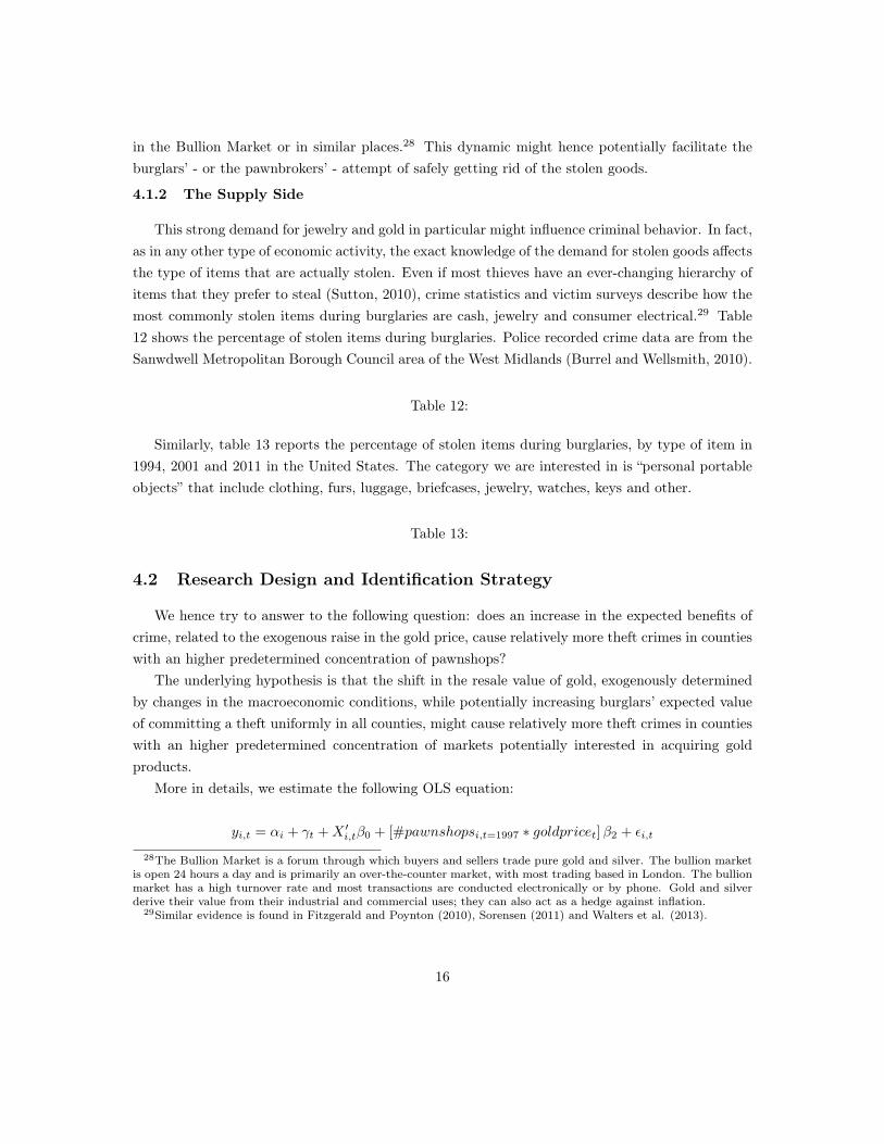
We hence try to answer to the following question: does an increase in the expected benefits ofcrime, related to the exogenous raise in the gold price, cause relatively more theft crimes in countieswith an higher predetermined concentration of pawnshops?

The underlying hypothesis is that the shift in the resale value of gold, exogenously determinedby changes in the macroeconomic conditions, while potentially increasing burglars’ expected valueof committing a theft uniformly in all counties, might cause relatively more theft crimes in countieswith an higher predetermined concentration of markets potentially interested in acquiring goldproducts.

More in details, we estimate the following OLS equation:

yi,t = αi + γt +X ′i,tβ0 + [#pawnshopsi,t=1997 ∗ goldpricet]β2 + εi,t

28The Bullion Market is a forum through which buyers and sellers trade pure gold and silver. The bullion marketis open 24 hours a day and is primarily an over-the-counter market, with most trading based in London. The bullionmarket has a high turnover rate and most transactions are conducted electronically or by phone. Gold and silverderive their value from their industrial and commercial uses; they can also act as a hedge against inflation.

29Similar evidence is found in Fitzgerald and Poynton (2010), Sorensen (2011) and Walters et al. (2013).

16

where i indicates the county, s the state and t the year. Also in this case, the outcome of interestis the number of reported crimes, by county per year. The coefficient of interest is β2, the effect oncrime of the interaction between the initial concentration of the number of pawnshops per capitafixed in the first year of our sample (1997) and the gold price at time t. As in the first part of thepaper, standard errors are clustered at the county level.

As in the first part of the paper, we use a within county specification including county fixedeffect. A key role in this specification is played by the inclusion of year fixed effects, that partial outfrom the estimate the direct and uniform effect that the rise in gold price might have on the growthof theft crimes in all counties. Moreover, while arguably gold price is related to the stability of theglobal economic conditions, our specification uses a wide set of socio - economic controls related tothe conditions of the local economy. As in the first part of the paper we include all controls andalso the contemporaneous number of pawnshops. Furthermore, in order to control for the presenceof other possible time - varying confounding factors, we add the interaction between each controlfixed in year 1997 and the price of gold.30

Importantly for our analysis this specification - while providing a different angle from whichanalysing the role of stolen goods markets on crime - it also unambiguosly addresses the reversecausality issue underlined in the first part of the paper.

4.2.1 The Evolution of Gold Price

This study focuses on a 14 years period, from 1997 to 2010. During this period, gold pricedisplayed some positive and negative oscillation, nevertheless raising its value of about 37% from1997 to 2005. From 2006 to 2010 instead, gold price experienced an impressive increase of almost200%.31

Figure 4.1:

This huge final spike poses some empirical issue that we address dividing the analysis in twoperiods:1997-2005 and 2006-2010. In particular, we are worried that the spike of almost 40% inthe value of gold from 2006 to 2005 pushed other type of businesses such as jewelries and onlinerefineries to increase the demand for gold products. In this case, the number of pawnshops, ameasure of the underlying size of the market for gold, would suffer from a downward bias thatwould be amplified by the increase in measurement error after 2005.

30 Results are qualitatively unchanged if we allow all the the controls to vary with the gold price.

31I use as unit of measurement the price of gold in US dollars (averaged over the entire year) per troy ounce. Dataare freely downloadable at the following website: http://www.gold.org.

17

4.2.2 Results

Tables 14 and 15 reports the results, both for theft crimes and other crimes. The first row showsthe effect of the contemporaneous number of pawnshops, while the second row reports the resultsof the interaction term of interest.

Table 14:

Overall, the estimates confirm the prediction that the effect of pawnshops on crime was strongand highly significant in the first 9 years of the sample rather that in the last 5. In particular,the main effect of pawnshops on larcenies and burglaries is 6.17 and 2.13, with both coefficientssignificant at the 1%. Converesly, these coefficients estimated in the second part of the panelare not precisely estimated. Furthermore, we detect a positive effect of the interaction term onlyfor buglaries for both periods of the sample, of 1.10 and 0.30 both significant at the 10% level.To put this result into perspective, a one standard deviation increase in the initial concentrationof pawnshops generates a 0.05 to 0.10 standard deviation increase in the effect of gold price onburglaries.

This time, the effect of the interaction term on larceny is not precisely estimated. These mightbe due to the fact that jewelry is a rare outcome for this generic type of theft, that includes theftsof bicycles, motor vehicle parts and accessories, shoplifting, pocket-picking, or the stealing of anyproperty or article that is not taken by force. Once again, to further validate our analysis, no effectis detected on all other crimes (Table 15).

Table 15:

4.2.3 Robustness Checks

Table 16 shows the set of robustness checks for burglary between 1997 - 2005 (Panel A) and2006 - 2010 (Panel B).

Table 16:

Column 1 reports the coefficient when we cluster standard errors at the state level, while incolumn 2 we show the results with double clustering at county - year level. For both the samples weloose precision in the estimates. As in the first part of the paper, column 3 shows the results whenwe weight the regression by the coverage indicator, in column 4 and 5 we eliminate respectively thecounties in the top 1% of the pawnshops and population distribution. Coefficients are stable acrossall different specifications, with the only exception being column 4 panel B, with a p - value of 11%.

18

4.2.4 Copper Thefts and the “Red Gold” Rush

The demand for copper from developing nations has generated an intense international coppertrade. According to the FBI, copper thieves are exploiting this demand and the related spike ininternational prices by stealing and selling the metal to recyclers across the United States. Copperthieves are targeting electrical sub-stations, cellular towers, telephone land lines, railroads, waterwells, construction sites, and vacant homes for lucrative profits.

In this last part of the paper we hence decide to perform a further falsification test, exploitingthe fact that objects made by copper - while being heavily targeted by criminals - are not usuallyaccepted in pawnshops’ transactions. Table 17 shows the results when we include in the specificationthe interaction between the price of copper an the initial concentration of pawnshops in the county.32

Table 17:

Adding this further control generates a multicollinearity between the two interaction term thatreduces the significance of the interaction between gold price and pawnshops. 33 As we wereexpecting, we do not detect any positive effect of the initial concentration of pawnshops on theeffect of copper price on burglaries. Interestingly, we instead detect a negative coefficient of 1.8significant at the 1% level in the second part of the sample. While we do not want to overemphasizesthis result, we consider the substituability across market for stolen goods as an extremely interestingvenue for future research.

5 Concluding Remarks

This paper has offered a systematic empirical investigation of the effect of stolen goods marketson crime, an issue never properly explored in the existing literature on the determinants of crime.In particular, motivated by the richness of anecdotal evidence, we have looked at this issue troughthe lens of pawnshops, a business that has long being suspected of illicit trade. The endogeneity ofpawnshops to crime has been addressed in multiple ways.

In the first part of the paper we have mainly exploited the panel properties of the data. Re-sults confirm that the number of pawnshops is a strong and significant predictor of larcenies andburglaries. The findings are robust to extensive robustness checks, the clustering of standard er-rors at a different levels, the sensitivity to outliers, averaging the regression by a measure of thequality of the information available to the researcher and using a log - log model. The mechanismbehind the findings is validated by numerous falsification tests on other crimes that disprove thepossibility that pawnshops might affect crime trough channels other than the transaction of stolen

32Data on historical copper price is obtained through the U.S. geological survey at: http://www.usgs.gov/33The correlation between the price of gold and copper is 0.84.

19

goods. Moreover, we have detected the presence of geographical spillover effects on crime and wehave analyzed the heterogeneity in the results across counties with a different population density.

In the second part of the paper we have exploited the exogenous shift in crimes’ expected benefitsusing the raise in gold price - the main determinant of pawnbrokers’ profit function - as a quasinatural experiment, where the intensity of the treatment is given by the initial concentration ofpawnshops in the county. In particular, the identification strategy relied on the exogeneity of theinteraction between the price of gold, constantly demanded by pawnbrokers in the form of jewelsthat are usually melted down to be transformed into a bar of the precious metal, and the initialallocation of the number of pawnshops in the county. A one standard deviation increase in theinitial concentration of pawnshops generates a 0.05 to 0.10 standard deviation increase in effectof gold on burglaries. Also in this case, results are robust to a wide set of robustness checks andare corroborated by the presence of falsification tests on crimes that should not be affected by thepresence of pawnshops.

This paper offers new direction of future research. A direct spin off of this work would be theanalysis of other possible market for stolen goods, such as flea markets, junkyards and online websites such as Ebay or Craigslist. Moreover, entering in the “black box” of the mechanism that linksdemand and supply of crime is critical for the understanding of criminal behavior. Two mechanismsmight in fact play an important role in this context. On the one hand, the increase in the size ofstolen goods’ markets might increase crime by reducing the criminal expected probability of beingarrested (negative deterrence effect). On the other hand, the increase in the level of competition inthe resale market might push up prices, raising the expected resale value of the stolen item (priceeffect). Disentangling these two channels might help shaping specific policy interventions orientedto reduce the impact that the proliferation of stolen goods markets can have on crime. This andother interesting aspects are left for future research.

References

1. Altonji, Joseph G., Todd E. Elder, and Christopher R. Taber, \Selection on Observed andUnobserved Variables: Assessing the Effectiveness of Catholic Schools," Journal of PoliticalEconomy, February 2005, 113 (1), 151 -184.

2. Avery, Robert B., and Katherine Samolyk. "Payday loans versus pawnshops: The effects ofloan fee limits on household use." Federal Reserve System, Working Paper (2011).

3. Bayer, Patrick, Randi Hjalmarsson, and David Pozen, “Building Criminal Capital BehindBars: Peer Effects in in Juvenile Corrections,” Quarterly Journal of Economics, February2009, 124 (1).

20

4. Becker, Gary S., “Crime and Punishment: An Economic Approach,” Journal of PoliticalEconomy, March/April 1968, 76 (2), 169–217.

5. Bianchi, Milo, Paolo Buonanno, and Paolo Pinotti. "Do immigrants cause crime?." Journalof the European Economic Association 10.6 (2012): 1318-1347.

6. Bhuller, Manudeep, Havnes, Tarjei , Leuven, Tarjei and Mogstad, Magne, “Broadband Inter-net: An Information Superhighway to Sex Crime?”, Review of Economic Studies, 80, 1237-1266, 2013.

7. Case, Anne C. and Lawrence F. Katz, “The Company You Keep: The Effects of Family andNeighborhood on Disadvantaged Youths,” NBER Working Paper #3705, 1991.

8. Caskey, John P. "Fringe banking and the rise of payday lending." Credit markets for the poor,17 (2005): 18-19.

9. Comeau, Michelle, Klofas, John “Analysis of 2011 Rochester City Pawn Shop Transactions:The Year in Review”, Center for Public Safety Initiatives, Working Paper, 2012.

10. Dahl, Gordon, and Stefano DellaVigna. "Does movie violence increase violent crime?." TheQuarterly Journal of Economics 124.2 (2009): 677-734.

11. Di Tella, Rafael and Ernesto Schargrodsky, “Do Police Reduce Crime? Estimates Using theAllocation of Police Forces After a Terrorist Attack,” American Economic Review, March2004, 94 (1), 115–133.

12. Donohue, John J., III and Steven J. Levitt, “The Impact of Legalized Abortion on Crime,”Quarterly Journal of Economics, May 2001, 116 (2), 379–420.

13. Draca, Mirko, Stephen Machin, and Robert Witt. "Panic on the streets of London: Police,crime, and the july 2005 terror attacks." The American Economic Review 101.5 (2011): 2157-2181.

14. Drago, Francesco, Roberto Galbiati, and Pietro Vertova, “The Deterrent Effects of Prison:Evidence from a Natural Experiment,” Journal of Political Economy, 2009, 117 (2), 257–280.

15. Eeckhout, Jan, Nicola Persico, and Petra E. Todd. "A theory of optimal random crackdowns."The American Economic Review 100.3 (2010): 1104-1135.

16. Fass, Simon M., and Janice Francis. "Where have all the hot goods gone? The role ofpawnshops." Journal of Research in Crime and Delinquency 41.2 (2004): 156-179.

17. Fellowes, Matthew, and Mia Mabanta. Banking on wealth: America’s new retail bankinginfrastructure and its wealth-building potential. Brookings Institution, 2008.

21

18. Fitzgerald, Jacqueline, and Suzanne Poynton. "The changing nature of objects stolen inhousehold burglaries." Crime and Justice Statistics: Bureau Brief 62 (2011): 1-12.

19. Florida Committee on Criminal Justice. 2000. “A Review of Florida’s Pawnbroking Law.” TheFlorida Senate, Committee on Criminal Justice (Interim Project Report 2000-26).Washington,DC: Government Printing Office.

20. Gaviria, Alejandro and Steven Raphael, “School-Based Peer Effects and Juvenile Behavior,”Review of Economics and Statistics, May 2001, 83 (2), 257–268

21. Glaeser, Edward L. and Bruce Sacerdote, “Why is There More Crime in Cities?,” Journal ofPolitical Economy, December 1999, 107 (2, Part 2), S225–S258

22. Glaeser, Edward, Bruce Sacerdote and Jose A. Scheinkman, “Crime and Social Interactions,”Quarterly Journal of Economics, May 1996, 111 (2), 507–548.

23. Glover, S. and E. Larrubia. 1996,November 24. “A System in Hock: Quick Cash with FewQuestions.” South Florida Sun-Sentinel, p. 22A.

24. Grogger, Jeff, “The Effect of Arrests on the Employment and Earnings of Young Men,” Quar-terly Journal of Economics, February 1995, 110 (1), 51–72.

25. Grogger, Jeff, “Market Wages and Youth Crime,” Journal of Labor Economics, October 1998,16 (4), 756–791.

26. Hammond,B. 1997, December 3. “Pawnshops Link Addicts and Crime.” The Oregonian, p.5A.

27. Helland, Eric and Alex Tabarrok, “Does Three Strikes Deter: A Non-Parametric Investiga-tion,” Journal of Human Resources, Spring 2007, 42 (2), 309–330.

28. Jacob, Brian A. and Lars Lefgren, “Are Idle Hands the Devil’s Workshop? Incapacitation,Concentration and Juvenile Crime,” American Economic Review, December 2003, 93 (5),1560–1577.

29. Katz, Lawence F., Steven D. Levitt, and Ellen Shustorovich, “Prison Conditions, CapitalPunishment and Deterrence,” American Law and Economics Review, Fall 2003, 5 (2), 318–343.

30. Klick, Jonathan and Alexander Tabarrok, “Using Terror Alert Levels to Estimate the Effectof Police on Crime,” Journal of Law and Economics, April 2005, 48.

31. Kling, Jeffrey R., “Incarceration Length, Employment, and Earnings,” American EconomicReview, June 2006, 96 (3), 863–876.

22

32. Kling, Jeffrey, Jens Ludwig, and Lawrence F. Katz, “Neighborhood Effects on Crime for Fe-male and Male Youth: Evidence from a Randomized Housing Voucher Experiment,” QuarterlyJournal of Economics, February 2005, 120 (1), 87–130.

33. Kuziemko, Ilyana. Going off parole: How the elimination of discretionary prison release affectsthe social cost of crime. No. w13380. National Bureau of Economic Research, 2007.

34. Lee, David S. and Justin McCrary, “Crime, Punishment, and Myopia,” NBER Working Paper# 11491, July 2005

35. Levitt, Steven D., “The Effect of Prison Population Size on Crime Rates: Evidence from PrisonOvercrowding Litigation,” Quarterly Journal of Economics, May 1996, 111 (2), 319–351.

36. Levitt, Steven D., “Using Electoral Cycles in Police Hiring to Estimate the Effect of Police onCrime,” American Economic Review, June 1997, 87 (3), 270–290.

37. Levitt, Steven D., “Juvenile Crime and Punishment,” Journal of Political Economy, December1998, 106 (6), 1156–1185.

38. Levitt, Steven D.,“Understanding Why Crime Fell in the 1990s: Four Factors that Explainthe Decline and Six that Do Not,” Journal of Economic Perspectives, Winter 2004, 18 (1),163–190.

39. Lochner, Lance and Enrico Moretti, and Enrico Moretti, “The Effect of Education on Crime:Evidence from Prison Inmates, Arrests, and Self-Reports,” American Economic Review, March2004, 94 (1), 155–189.

40. Miles, Thomas J. “Markets for Stolen Property: Pawnshops and Crime”, (unpublished disser-tation chapter), 2007.

41. Nunn, Nathan and Leonard Wantchekon, “The Slave Trade and the Origins of Mistrust inAfrica," American Economic Review, 2012, 101 (7), 3221 - 52.

42. Paige, Skiba , Marieke Bos, and Susan Carter. "The Pawn Industry and Its Customers: TheUnited States and Europe." Vanderbilt Law and Economics Research Paper, 12-26 (2012).

43. Polinsky, A. Mitchell and Steven Shavell, “The Economic Theory of Public Enforcement ofLaw,” Journal of Economic Literature, March 2000, 38 (1), 45–76.

44. Raphael, Steven and Rudolf Winter-Ebmer, “Identifying the Effect of Unemployment onCrime,” Journal of Law and Economics, April 2001, 44 (1), 259–284.

45. Scott, D. 1992, June 26. “Pawnshops Multiply Despite Seedy Image: Big Chains GobbleMomand- Pops, Spawn Industry Transformation.” Dallas Business Journal, pp. 1, 54-55.

23

46. Shackman, Joshua D., and Glen Tenney. "The Effects of Government Regulations on theSupply of Pawn Loans: Evidence from 51 Jurisdictions in the US." Journal of FinancialServices Research 30.1 (2006): 69-91. APA

47. Silverman, Dan, “Street Crime and Street Culture,” International Economic Review, August2004, 45 (3), 761–786.

48. Sorensen, David WM. Rounding up Suspects in the Rise of Danish Burglary: A StatisticalAnalysis of the 2008/09 Increase in Residential Break-ins. Justitsministeriet, 2011.

49. Sutton, Michael. Stolen Goods Markets. US Department of Justice, Office of CommunityOriented Policing Services, 2010.

50. Walters, Jennifer Hardison, Andrew Moore, M. Stat, Marcus Berzofsky, and Lynn Langton."Household Burglary, 1994-2011."

51. Warner, Bill. "No Questions Asked: Sarasota Pawn Shop Businesses Charged in Sting Oper-ation, Black-Market Fencing Easy Cash For Burglars & Armed Robbers." April 25, 2011.

52. Wellsmith, Melanie, and Amy Burrell. "The Influence of Purchase Price and OwnershipLevels on Theft Targets The Example of Domestic Burglary." British Journal of Criminology45.5 (2005): 741-764.

53. Western, Bruce, Jeffrey R. Kling, and David F. Weiman. "The labor market consequences ofincarceration." Crime & delinquency 47.3 (2001): 410-427.

54. Wheat, W. J. 1998. “A Study on the Status of the Pawnbrokers Industry in the State ofOklahoma.” Consumer Finance Law Quarterly Report 52:87-92.

55. Wright, Richard T. and Scott H. Decker. 1994. Burglars on the Job: Streetlife and ResidentialBreak-ins. Boston: Northeastern University Press.

Data Appendix

Crimes Definition

1. Murder (criminal homicide): The willful (non negligent) killing of one human being byanother.

2. Forcible rape: The carnal knowledge of a female forcibly and against her will.

24

3. Robbery: The taking or attempting to take anything of value from the care, custody, orcontrol of a person or persons by force or threat of force or violence and/or by putting the victimin fear.

4. Aggravated assault: An unlawful attack by one person upon another for the purpose of ininflicting severe or aggravated bodily injury. This type of assault usually is accompanied by the useof a weapon or by means likely to produce death or great bodily harm.

5. Burglary: The unlawful entry of a structure to commit a felony or a theft.6. Larceny: The unlawful taking, carrying, leading, or riding away of property from the posses-

sion or constructive possession of another. Common types of larcenies include shoplifting, pocket-picking, purse snatching, theft of objects from motor vehicles, theft of bicycles and theft of itemsfrom buildings in which the offender has legal access.

7. Motor vehicle theft: The theft or attempted theft of a motor vehicle.8. Arson: any willful or malicious burning or attempting to burn, with or without intent to

defraud, a dwelling house, public building, motor vehicle or aircraft, personal property of another,etc.

Hierarchy Rule

In some cases, a single incident may have consisted of two distinct offenses. For example, duringthe course of a robbery, a victim may have been fatally shot. In cases in which multiple offenses arecommitted by the same offender against the same victim during a given felonious act, the hierarchyrule is employed to determine how the crime is classified. A crime is classified according to themost serious offense committed. Importantly, the hierarchy rule does not apply to the offense ofarson. In fact, when arson is involved in a multiple offense situation, the reporting agency mustreport two part I offenses, the arson as well as the additional part I offense.

25

 

Table 1 Descriptive Statistics (Pawnshops and Crime Related)

(1) (2) (3) (4) (5) Observations Mean Standard Dev Min Max Pawnshops 28,430 5.88 6.325 0 112.9

Larcenies 28,430 1,840 1,046 0 12,073 Burglaries 28,430 654.2 394.7 0 2,960 Robberies 28,430 52.74 73.96 0 822.4 Motor/Vehicle Thefts 28,430 190.4 180.0 0 2,385

Murders 28,430 3.86 5.43 0 128.9 Rapes 28,430 27.28 22.44 0 513.5 Assaults 28,430 237.2 203.2 0 2,676 Arsons 28,430 18.13 20.81 0 604.2

Notes: Variables normalized per 100.000 people

 

 

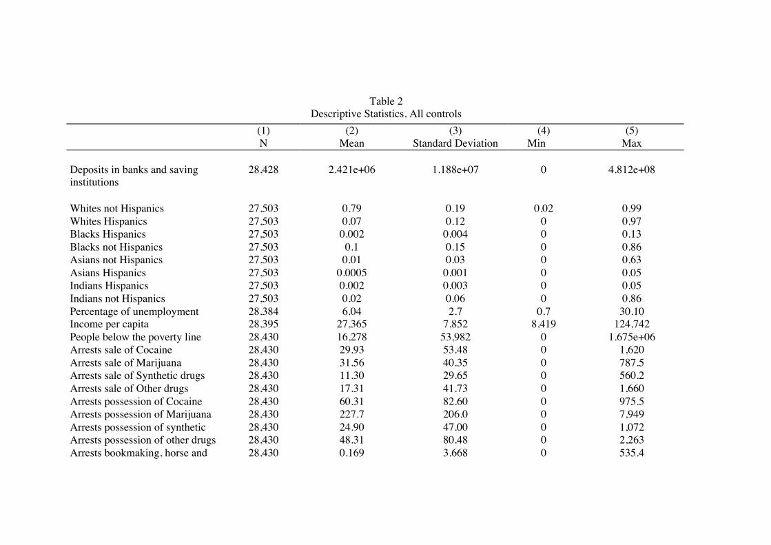
Table 2

Descriptive Statistics, All controls (1) (2) (3) (4) (5) N Mean Standard Deviation Min Max Deposits in banks and saving institutions

28,428 2.421e+06 1.188e+07 0 4.812e+08

Whites not Hispanics 27,503 0.79 0.19 0.02 0.99 Whites Hispanics 27,503 0.07 0.12 0 0.97 Blacks Hispanics 27,503 0.002 0.004 0 0.13 Blacks not Hispanics 27,503 0.1 0.15 0 0.86 Asians not Hispanics 27,503 0.01 0.03 0 0.63 Asians Hispanics 27,503 0.0005 0.001 0 0.05 Indians Hispanics 27,503 0.002 0.003 0 0.05 Indians not Hispanics 27,503 0.02 0.06 0 0.86 Percentage of unemployment 28,384 6.04 2.7 0.7 30.10 Income per capita 28,395 27,365 7,852 8,419 124,742 People below the poverty line 28,430 16,278 53,982 0 1.675e+06 Arrests sale of Cocaine 28,430 29.93 53.48 0 1,620 Arrests sale of Marijuana 28,430 31.56 40.35 0 787.5 Arrests sale of Synthetic drugs 28,430 11.30 29.65 0 560.2 Arrests sale of Other drugs 28,430 17.31 41.73 0 1,660 Arrests possession of Cocaine 28,430 60.31 82.60 0 975.5 Arrests possession of Marijuana 28,430 227.7 206.0 0 7,949 Arrests possession of synthetic 28,430 24.90 47.00 0 1,072 Arrests possession of other drugs 28,430 48.31 80.48 0 2,263 Arrests bookmaking, horse and 28,430 0.169 3.668 0 535.4

 

sport Arrests numbers and lotteries 28,430 0.10 1.30 0 106.7 Arrests other gambling 28,430 1.70 13.26 0 1,327 Rate of Poverty 28,430 0.14 0.06 0 0.50 Number of social security recipients

28,430 20,488 47,166 0 1.148e+06

Total number of police officers in the state at t-1

28,429 94.98 52.53 0 286.5

Density 28,421 318.5 2,019 0.194 67,589

 

TABLE 3 Theft Crimes vs. Other Crimes

(1) (2) (3) (4) (5) (6) (7) (8) (9) (10) Theft Crimes (Grouped) Other Crimes (Grouped) Pawnshops per capita 18.28*** 16.74*** 26.85*** 6.475*** 6.070*** 3.119*** 3.002*** 2.440*** 0.00386 0.0562 (5.540) (5.472) (6.776) (2.134) (2.167) (0.668) (0.663) (0.626) (0.493) (0.493) Observations 28,430 28,430 28,430 28,430 27,466 28,430 28,430 28,430 28,430 27,466 Adjusted R-squared 0.006 0.021 0.160 0.850 0.856 0.008 0.013 0.310 0.724 0.738 YEAR FE NO YES YES YES YES NO YES YES YES YES STATE TRENDS NO NO YES YES YES NO NO YES YES YES COUNTY FE NO NO NO YES YES NO NO NO YES YES Controls NONE NONE NONE NONE ALL NONE NONE NONE NONE ALL *** p<0.01, ** p<0.05, * p<0.1. Standard errors are clustered at the county level. The number of pawnshops and reported crimes are expressed in per capita terms. The unit of analysis is the county. Theft Crimes include: larcenies, robberies, burglaries and motor – vehicle thefts. Other crimes include: murders, rapes, aggravated assaults and arsons. The table shows the evolution of the coefficients when fixed effects and controls are included. The most complete specification (with county FE, year FE, State linear trends and all controls) is shown in column 5 and 10.

 

TABLE 4 Crimes Breakdown

(1) (2) (3) (4) (5) (6) (7) (8) Larcenies Burglaries Robberies M-V Thefts Murders Rapes Assaults Arsons Pawnshops per capita 4.572*** 1.518** -0.0249 0.00530 0.0160 0.0251 -0.0409 0.0560 (1.675) (0.652) (0.0580) (0.172) (0.0196) (0.0523) (0.469) (0.0413) Observations 27,466 27,466 27,466 27,466 27,466 27,466 27,466 27,466 Adjusted R-squared 0.842 0.796 0.917 0.845 0.285 0.541 0.728 0.510 Year FE YES YES YES YES YES YES YES YES State Trends YES YES YES YES YES YES YES YES County FE YES YES YES YES YES YES YES YES Controls ALL ALL ALL ALL ALL ALL ALL ALL

*** p<0.01, ** p<0.05, * p<0.1. All the standard errors are clustered at the county level. The table shows the results from 8 different regressions, one for each type of reported crime. All the specifications include county FE, year FE, state trends and all controls.

 

TABLE 5 Crimes Breakdown – Log/Log Specification

(1) (2) (3) (4) (5) (6) (7) (8) Larcenies Burglaries Robberies M-V Thefts Murders Rapes Assaults Arsons Pawnshops per capita 1.487** 0.828** -0.0267 0.00484 0.0152 -0.0163 0.0288 0.0528 (0.714) (0.400) (0.0539) (0.138) (0.0193) (0.330) (0.0490) (0.0399) Observations 27,466 27,466 27,466 27,466 27,466 27,466 27,466 27,466 Adjusted R-squared 0.829 0.792 0.916 0.849 0.287 0.747 0.548 0.522 Year FE YES YES YES YES YES YES YES YES State Trends YES YES YES YES YES YES YES YES County FE YES YES YES YES YES YES YES YES Controls ALL ALL ALL ALL ALL ALL ALL ALL

*** p<0.01, ** p<0.05, * p<0.1. All the standard errors are clustered at the county level. The table shows the results from 8 different regressions, one for each type of reported crime. All the specifications include county FE, year FE, state trends and all controls. Variables of interest are computed as ln(0.01 + x), where x is the percapita value of the variable.

 

TABLE 6 Pawnshops’ lagged structure

(1) (2) (3) (1) (2) (3) Larcenies Burglaries Pawnshops per capita 4.57*** 2.96** 2.58* 1.51** 0.31 0.13 (1.67) (1.38) (1.330) (0.65) (0.55) (0.520) Pawnshops per capita (T-1) 1.38 0.044 1.24* 0.46 (1.62) (1.318) (0.67) (0.565) Pawnshops per capita (T-2) 2.07 0.87 (1.39) (0.63) Year FE YES YES YES YES YES YES State Trends YES YES YES YES YES YES County FE YES YES YES YES YES YES Controls ALL ALL ALL ALL ALL ALL

*** p<0.01, ** p<0.05, * p<0.1. All the standard errors are clustered at the county level. In both columns 1, both for larcenies and burglaries, we show the baseline specification with the contemporaneous number of pawnshops. In columns 2 we add the number of pawnshops per capita, at t-1. Finally, in columns 3 we include the number of pawnshops per capita at t-2.

 

TABLE 7 Crimes’ lagged structure (Pawnshops as an outcome)

(1) (2) (3) (4) (5) (6) Larcenies Burglaries Contemporaneous Crime 0.25*** 0.12 0.11 0.46** 0.18 0.09 (0.9) (0.08) (1.330) (0.20) (0.17) (0.18) Crime (T-1) 0.17** 0.10* 0.29* 0.21 (0.08) (1.318) (0.17) (0.15) Crime (T-2) 0.11 0.11 (1.39) (0.17) Year FE YES YES YES YES YES YES State Trends YES YES YES YES YES YES County FE YES YES YES YES YES YES Controls ALL ALL ALL ALL ALL ALL

*** p<0.01, ** p<0.05, * p<0.1. All the standard errors are clustered at the county level. The outcome variable is the number of pawnshops per capita in the county at time t. In the first three columns the main regressor is the number of larcenies. In the last three columns the coefficient of interest is the number of burglaries.

 

TABLE 8 Robustness Checks

(1) (2) (3) (4) (5)

Panel A - Larcenies

Pawnshops per capita 4.57** 4.57*** 4.37*** 4.94*** 4.53***

(2.1) (1.59) (1.569) (1.761) (1.68)

Panel B - Burglaries

Pawnshops per capita 1.51** 1.51** 1.48** 1.6** 1.51**

(0.65) (0.73) (0.62) (0.68) (0.65)

Year FE YES YES YES YES YES State Trends YES YES YES YES YES County FE YES YES YES YES YES Controls ALL ALL ALL ALL ALL *** p<0.01, ** p<0.05, * p<0.1. Panel A shows the results for larcenies, while panel B shows the results for burglaries. Column 1 shows the results when we cluster at the state level, while in column 2 we cluster at the county/year level. In column 3 we perform a weighted regression using as weight the FBI coverage indicator. In column 4 we eliminate from the sample the counties in the top 1% of the pawnshops’ per capita distribution. In column 5 we eliminate from the sample the counties in the top 1% of the population distribution.

 

TABLE 9 Heterogeneity in the Results: Density

(1) (2) (3) (4) (5) (6) (7) (8) Larcenies

Low High Burglaries

Low High Robberies

Low High M/V Thefts

Low High Pawnshops per capita 3.36* 10.4*** 1.32* 2.77* -0.05 0.11 0.09 -0.0657 (1.97) (3.7) (0.74) (1.34) (0.0597) (0.163) (0.198) (0.467) Observations 13,788 13,678 13,788 13,678 13,788 13,678 13,788 13,678 Year FE YES YES YES YES YES YES YES YES State Trends YES YES YES YES YES YES YES YES County FE YES YES YES YES YES YES YES YES Controls ALL ALL ALL ALL ALL ALL ALL ALL

*** p<0.01, ** p<0.05, * p<0.1. Standard errors clustered at the county level. The sample is divided in counties below the median density and above the median density. The density percentiles are computed with respect to the density of the county, averaged for each county in the 14 years of the sample (1997 - 2010).

 

TABLE 10

Geographical Spillovers (1) (2) (3) (4) Larcenies Burglaries Robberies M/V Thefts Pawnshops (Same County) 4.53*** 1.49** -0.026 0.000 (1.66) (0.65) (0.0588) (0.17)

Pawnshops (Bordering Counties) -0.2 0.22 -0.12 0.03 (2.3) (1.019) (0.11) (0.33)

Pawnshops (State Level) 21.60* 15.1*** 0.94* 2.38 (12.01) (4.3) (0.54) (1.90) Observations 27,450 27,450 27,450 27,450 Adjusted R-squared 0.85 0.799 0.912 0.842 Year FE YES YES YES YES State Trends YES YES YES YES County FE YES YES YES YES Controls ALL ALL ALL ALL

*** p<0.01, ** p<0.05, * p<0.1. All the standard errors are clustered at the county level. Each column shows the results from a different regression where the outcome variable is the number of reported crimes (per capita) in the county. In each regression we include the number of pawnshops in the county, the number of pawnshops in the bordering counties (excluding the number of pawnshops in the county where crime is measured), the number of pawnshops in the state (excluding the number of pawnshops in the county where crime is measured).

 

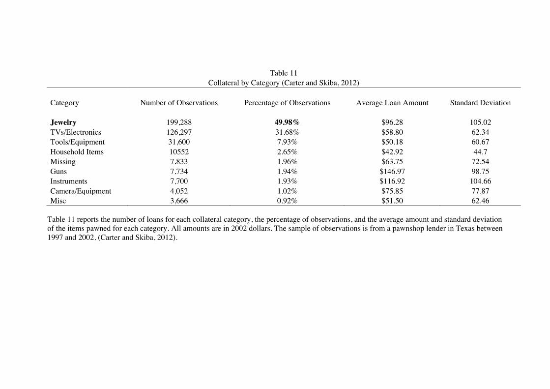
Table 11

Collateral by Category (Carter and Skiba, 2012)

Category Number of Observations Percentage of Observations Average Loan Amount Standard Deviation

Jewelry 199,288 49.98% $96.28 105.02 TVs/Electronics 126,297 31.68% $58.80 62.34 Tools/Equipment 31,600 7.93% $50.18 60.67 Household Items 10552 2.65% $42.92 44.7 Missing 7,833 1.96% $63.75 72.54 Guns 7,734 1.94% $146.97 98.75 Instruments 7,700 1.93% $116.92 104.66 Camera/Equipment 4,052 1.02% $75.85 77.87 Misc 3,666 0.92% $51.50 62.46

Table 11 reports the number of loans for each collateral category, the percentage of observations, and the average amount and standard deviation of the items pawned for each category. All amounts are in 2002 dollars. The sample of observations is from a pawnshop lender in Texas between 1997 and 2002, (Carter and Skiba, 2012).

 

Table 12 (Burrel and Wellsmith, 2010) Items stolen during burglaries

Cash 40%

Documents 5% Jewellery 31%

Ornaments 5%

Audio 25%

Food 5% VCR 17%

Tools 5%

TV 17%

Furniture 3% Personal 12%

Cigarettes 3%

Telecom 12%

Vehicles 2% Computer 11%

Cycle 2%

Photographic 11%

DVD 2% Games 10%

Building 1%

Purse 10%

Garden 1% Cards 10%

Digital 0%

Luggage 9%

Sports 0% Clothing 9%

Antiques 0%

Domestic 7% Keys 6%

This table shows the percentage of the stolen items during burglaries. Police recorded crime data are from the Sanwdwell Metropolitan Borough Council area of the West Midlands. The period covered is from 1997 to 2003. Percentage do not sum to 100 due to the stealing of multiple categories.

 

Table 13 Items taken during completed household burglaries, by type of item

1994 2001 2011

Number Per cent Number Per cent Number Per cent

Total completed burglaries 5,261,200

3,067,800

2,845,500

Cash/checks, credit/bank cards, purses/wallets 786,600 15 553,200 18 482,200 16.9 Motor vehicles 33,400 0.6 33,400 1.1 38,600 1.4 Motor vehicle parts/accessories, gasoline/oil 217,300 4.1 130,800 4.3 128,500 4.5 Bicycles or parts, toys, recreation/sport equipment 698,600 13.3 382,700 12.5 246,500 8.7 Household appliances/portable electronics 1,433,900 27.3 844,400 27.5 978,700 34.4 Household furnishings/collections 359,000 6.8 225,300 7.3 179,100 6.3 Personal portable objects 1,482,600 28.2 905,400 29.5 885,200 31.1 Firearms 161,000 3.1 116,500 3.8 81,900 2.9 Tools/miscellaneous equipment 776,500 14.8 448,200 14.6 462,100 16.2 Farm/garden produce, food/liquor 272,900 5.2 169,700 5.5 129,200 4.5 Animals 21,700 0.4 2,800 0.1 3,500 0.1 Other 322,300 6.1 173,500 5.7 86,000 3 Unknown 11,000 0.2 7,400 0.2 7,300 0.3

This table shows the percentage of the stolen items during burglaries, by type of item in 1994, 2001 and 2011. Personal portable objects include clothing, furs, luggage, briefcases, jewelry, watches, keys and other. Source: Bureau of Justice Statistics, National Crime Victimization Survey, 1993 – 2011.

 

TABLE 14 Response to Gold Price (Theft Crimes)

(1) (2) (3) (4) (5) (6) (7) (8) Larcenies

1997-2005 2006-2010 Burglaries

1997-2005 2006-2010 Robberies

1997-2005 2006-2010 M/V Theft

1997-2005 2006-2010 Pawnshops per capita

6.17*** (1.77)

1.64 (1.73)

2.13*** (0.80)

0.92 (0.88)

0.9 (0.7)

-0.01 (0.08)

0.30 (0.24)

0.30 (0.26)

Pawnshops (t0)*Gold Price (t) -0.40 0.50 1.10* 0.30* 0.7 -0.02 -0.03 -0.02 (1.5) (0.38) (0.58) (0.16) (0.5) (0.02) (0.2) (0.05) Observations 17,195 10,271 17,195 10,271 17,195 10,271 17,195 10,271 Year FE YES YES YES YES YES YES YES YES County FE

YES YES

YES

YES

YES

YES

YES

YES

Controls ALL ALL ALL ALL ALL ALL ALL ALL Controls*Gold Price ALL ALL ALL ALL ALL ALL ALL ALL

*** p<0.01, ** p<0.05, * p<0.1. All the standard errors are clustered at the county level. This table shows the results of the specification where pawnshops per capita and the interaction between pawnshops in 1997 (the first year of the sample) and Gold price at time t are included. We also include the interactions between all controls fixed in the year 1997 and the gold price at time t, all controls, county and year fe.

 

TABLE 15 Response to Gold Price (Other Crimes)

(1) (2) (3) (4) (5) (6) (7) (8) Murders

1997-2005 2006-2010 Rape

1997-2005 2006-2010 Arson

1997-2005 2006-2010 Assaults

1997-2005 2006-2010 Pawnshops per capita

0.1 (0.2)

-0.00 (0.2)

0.05 (0.06)

-0.00 (0.9)

0.04 (0.05)

0.04 (0.08)

0.06 (0.53)

0.12 (0.55)

Pawnshops (t0)*Gold Price (t) -0.01 0.50 0.02 0.01 0.7 0.01 0.10 0.05 (0.01) (0.38) (0.04) (0.01) (0.5) (0.01) (0.38) (0.09) Observations 17,195 10,271 17,195 10,271 17,195 10,271 17,195 10,271 Year FE YES YES YES YES YES YES YES YES County FE

YES YES

YES

YES

YES

YES

YES

YES

Controls ALL ALL ALL ALL ALL ALL ALL ALL Controls*Gold Price ALL ALL ALL ALL ALL ALL ALL ALL

*** p<0.01, ** p<0.05, * p<0.1. All the standard errors are clustered at the county level. This table shows the results of the specification where pawnshops per capita and the interaction between pawnshops in 1997 (the first year of the sample) and Gold price at time t are included. We also include the interactions between all controls fixed in the year 1997 and the gold price at time t, all controls, county and year fe.

     

 

Table 16

Robustness Checks Burglaries (1) (2) (3) (4) (5)

Panel A – 1997-2005

Pawnshops (t0)*Gold Price (t) 1.10 1.10 1.18** 1.29** 1.09*

(0.66) (0.70) (0.58) (0.65) (0.58)

Panel B – 2006-2010

Pawnshops (t0)*Gold Price (t) 0.30 0.30 0.28* 0.27 0.29* (0.18) (0.19) (0.15) (0.18) (0.16)

*** p<0.01, ** p<0.05, * p<0.1. Panel A shows the results for larcenies, panel B shows the results for burglaries, panel C show the results for Robberies. Column 1 shows the results when we cluster at the state level, while in column 2 we cluster at the county/year level. In column 3 we perform a weighted regression using as weight the FBI coverage indicator. In column 4 we eliminate from the sample the counties in the top 1% of the pawnshops’ per capita distribution. In column 5 we eliminate from the sample the counties in the top 1% of the population distribution.

 

TABLE 17

Falsification Test on Copper Price (1) (2) Burglaries

1997-2005 2006-2010 Pawnshops (t0)*Gold Price (t) 1.26 0.20 (0.95) (0.16)

Pawnshops (t0)* Copper Price (t) -0.19 -1.8*** (0.90) (0.43)

Observations 17,195 10,271 Year FE Grouped YES YES County FE YES YES Controls ALL ALL Controls*Gold Price ALL ALL

*** p<0.01, ** p<0.05, * p<0.1. All the standard errors are clustered at the county level. In this specification we include the price of platinum and silver both interacted with the number of pawnshops in the first year of the sample.

 

Figure 3.1

 

Figure 4.1