DEPARTMENT OF ECONOMICS

Working Paper

The Real Exchange Rate as an Instrument of

Development Policy

by

Arslan Razmi, Martin Rapetti, and Peter Skott

Working Paper 2009-07

UNIVERSITY OF MASSACHUSETTS AMHERST

The Real Exchange Rate as an Instrument ofDevelopment Policy�

Arslan Razmiy, Martin Rapettiz and Peter Skottx

July 6, 2009

Abstract

Growth is endogenous in small open economies with substantial hiddenor open unemployment, even under constant returns to scale. Growthpromoting policies, however, have implications for the balance of trade,and two instruments are needed in order to achieve targets for both thegrowth rate and the balance of trade. The real exchange rate can serve asone of those instruments. Distributional con�ict imposes constraints onreal exchange rate policies, but in LDCs the main exchange-rate relateddistributional con�ict may be over the sectoral distribution of pro�ts,rather than the real wage. This paper develops a model along these linesand presents empirical support for the hypothesis that real exchange rateundervaluations are a useful instrument for the pursuit of accumulationand growth in low income countries.

JEL classi�cation: F43, O11, O41Key words: Real exchange rates, underemployment, capital accumu-

lation, investment, growth.

�An early version of this paper was presented at the Eastern Economic Association Meet-ings in New York, February 2009. We thank our discussant Jaime Ros for helpful commentsand suggestions.

yContact author: Department of Economics, University of Massachusetts Amherst,Amherst, MA 01003; email: arazmi@econs.umass.edu

zDepartment of Economics, University of Massachusetts Amherst, Amherst, MA 01003;email: mrapetti@econs.umass.edu

xDepartment of Economics, University of Massachusetts Amherst, Amherst, MA 01003;email: pskott@econs.umass.edu

1 Introduction

Growth is endogenous in a dual economy without full employment, as evidencedfor instance by the classic Harrod-Domar and Lewis models. This endogeneityof the growth rate also applies to open economies. In open economies, however,one needs to consider the implications of growth promoting policies for thebalance of trade. Our basic argument is simple: two instruments are needed inorder to achieve two targets (a growth rate and a balance of trade target). Thereal exchange rate can serve as one of those instruments.Most of contemporary economics assumes full employment, and those mod-

els that do include unemployment tend to play down the balance of paymentsconstraint and the role of the real exchange rate in this regard. We disagree withboth of these positions. Many developing economies have signi�cant amountsof (hidden) unemployment, and a recent empirical literature suggests that thereal exchange rate may have an important in�uence on long term economic per-formance. The precise mechanisms behind this in�uence, however, are unclear,and it is one of the aims of this paper to help �ll that gap.1

We set up a stylized model of a small open economy. The economy hastwo sectors, both with constant returns to scale. A modern sector produces atradable good while the output of a traditional sector is non-tradable. Onlythe former uses capital and all capital goods are imported. Assuming unem-ployment, we show that changes in the real exchange rate a¤ect the quantityand composition of employment and that the real exchange rate can be usedto facilitate sustained capital accumulation. Real exchange rate policies of thiskind have distributional e¤ects but in low income countries, we argue, the mainexchange-rate related distributional con�ict may be over the sectoral distribu-tion of pro�ts.Our empirical section focuses on the role of real exchange rate undervalu-

ations in promoting investment and output growth. We begin by replicatingthe results reported by Rodrik (2008). We �nd that Rodrik�s conclusion per-taining to di¤erences between developing and developed countries in the growthe¤ect of real exchange rate misalignments is sensitive to how these groups arede�ned in terms of income levels. We then create alternative classi�cationsand �nd that, in general, real exchange rate misalignments do appear to havea more signi�cant e¤ect on growth for developing countries. Our main empiri-cal contribution, however, is to analyze the relationship between real exchangerate changes and investment in light of our theoretical framework. We showthat real exchange rate undervaluations are (statistically) signi�cant drivers ofinvestment growth, but only in developing countries. This result is robust todi¤erent speci�cations, controls, and econometric methods.The paper falls in eight sections. Section 2 surveys relevant literature while

Section 3 provides some more context with the help of Chinese historical data.The benchmark model is presented in Section 4. We analyze the long-runimplications of the model in Section 5 and consider the short run in Section

1According to Eichengreen (2007) the literature has invested more in documenting thegrowth rate-real exchange rate correlation than in identifying channels of in�uence.

1

6. Section 7 discusses the econometrics and presents the results. Section 8concludes.

2 Literature Review

Macroeconomic analysis has traditionally played down the role of the exchangerate in causing or sustaining growth, although this may have recently begun tochange. The real exchange rate has been seen as an endogenous variable, itsvalue being determined in a general equilibrium set-up by �deeper�parameterssuch as preferences, factor endowments, and productivity, along with the levelof income of a country (the Balassa-Samuelson e¤ect). In the canonical (smallcountry) dependent economy framework, for example, the domestic price oftradables in domestic currency terms is determined internationally while theprice of non-tradables is determined by the deeper parameters. Developmenteconomists, on their part, may reject assumptions of purchasing power parityand full employment but, with important exceptions, have tended in the past toignore the potential role of the real exchange rate in development policy, perhapsdue to the traditional view of developing countries as exporters of primarycommodities and the resulting elasticity pessimism.The perceived irrelevance of policy in in�uencing exchange rates is now be-

ing challenged. A body of literature shows that the real exchange rate tracksthe nominal exchange rate quite closely over time which suggests that targetingthe latter may e¤ectively target the former as well, at least in the short- andmedium-run. Moreover, the ability of policy to in�uence the exchange rate inthe presence of capital mobility may have been underestimated. As illustratedby the Feldstein-Horioka puzzle, even assets from countries with completelyopen capital accounts appear not to be perfect substitutes (and capital con-trols seem to in�uence the nature if not magnitudes of capital �ows). Thecapital-account-openness vertex of the impossible trilemma is, therefore, lessbinding than would be the case in a world with unrestricted capital mobilityand negligible country risk premia. While the e¤ect of sterilized interventionsin developed countries is debatable, such interventions in developing countriesdo seem to have an impact, perhaps because international risk premia are higherfor developing country assets, and/or because foreign exchange markets tend tobe less deep in such countries.2 Thus, governments have a variety of policyoptions including monetary and �scal policy, saving incentives, capital controls,and reserve management, and the evidence suggests that governments do indeeduse several tools at their disposal to target exchange rates.Such policies can be e¤ective. Recent empirical studies of the role of compet-

itive exchange rates in promoting development have found a robust correlationbetween competitive exchange rates and economic growth.3 An interesting ex-

2See, for example Frenkel and Rapetti (2008) for a discussion of the Argentinean experienceof exchange rate management with sterilized interventions.

3See Razin and Collins (1997), Levi-Yeyati and Sturzeneggar (2007), Rodrik (2008), andthe literature cited below. A few recent studies have found a similar relationship between

2

ample is the study by Hausmann et al. (2005) which identi�ed and analyzeddeterminants of �growth episodes� in the latter half of the twentieth century.In other studies, Polterovich and Popov (2002) empirically identify exports asone of the channels through which competitive exchange rates correlate withproductivity and long term growth while Berg et al. (2008) �nd that episodesof growth in developing countries tend to be sustained and prolonged by com-petitive exchange rates and export diversi�cation.Rodrik (2008) �nds that (i) an undervaluation has a positive impact on the

size (and share) of output of the tradable sector in general and the industrialsector in particular, and (ii) the e¤ects of exchange rate changes on growth actsthrough the related change in the size of the tradable sector. Generally onewould expect an expansion of the tradable sector to be accompanied by greateremployment in that sector and, indeed, Galindo et al. (2001) and Frenkel andRos (2006) �nd that real exchange rate depreciations boost industrial employ-ment in samples of Latin American countries. Prasad et al. (2007a) reach thenear mirror image conclusion that foreign capital in�ows (roughly the �ip side ofcurrent account surpluses) tend to be associated with exchange rate overvalua-tion, which in turn has a detrimental e¤ect on sectoral allocation, manufacturedexports and growth (a form of the �Dutch disease�phenomenon).This emerging body of empirical evidence - along with East Asia�s rapid

accumulation of reserves in the pursuit of what is widely seen as �export-ledgrowth� - has stimulated interest in the theoretical linkages between the realexchange rate and growth. A common justi�cation for undervalued real ex-change rates is the need to shift resources toward the tradable sector, but ina traditional framework with full employment this begs the question of whatmakes the tradable sector special. Rodrik (2008) provides an answer in termsof market failures and endogenous growth. Production in the tradable sector,he argues, is especially a­ icted by institutional weaknesses and market failures(information and coordination externalities), and this leads to a bias againstthis sector in the allocation of resources. Exchange rate undervaluation boostspro�ts in the tradable sector and the resulting sectoral reallocation raises thegrowth rate in an AK-type model of endogenous growth.While Rodrik�s model focuses on sectoral di¤erences in the degree of insti-

tutional weakness, development economics has traditionally stressed both thelevel e¤ects of moving labor from low productivity sectors to the modern in-dustrial sector and dynamic e¤ects associated with greater scope for learningby doing (or other growth enhancing externalities) in the tradable sector. Evenif the magnitude of the externalities and scale e¤ects in the tradable sector isinsu¢ cient to allow for permanent endogenous growth, the scale e¤ects maygenerate multiple equilibria, and temporary exchange rate shocks can send theeconomy to a new long run equilibrium (Krugman, 1987; Ros and Skott, 1998).Some form of increasing returns, broadly interpreted, underpins these expla-

nations. An alternative macroeconomic justi�cation for undervalued exchange

real exchange rates and growth take-o¤ s on the one hand and real exchange rates and theduration of growth episodes on the other. See, for example, Hausmann et al. (2005) and Berget al. (2008).

3

rates is provided by Kaleckian models with underutilized resources. In this set-ting, a depreciation may boost aggregate demand (via the trade balance) andoutput in the short-run, and in a pro�t-led regime a real depreciation also stim-ulates growth due to the ensuing redistribution of income towards capitalists.4

Sectoral dimensions, however, tend to get ignored in the Kaleckian tradi-tion, and developing economies typically have dual labor markets with the trad-able goods being produced mainly in modern/urban/formal sectors and thenon-tradables in traditional/rural/informal sectors.5 Policies that bene�t thetradable sector have consequences for the distribution between wages, pro�ts,and land rents, as well as for distribution between workers in the two sectors.Most Kaleckian models pay little attention to these aspects, and the Kaleck-ian tradition, moreover, tends to emphasize quantity adjustments to externaldisequilibria over external relative price adjustments.The �balance of payments-constrained� growth model (BPCG), due origi-

nally to Thirlwall (1979), shares the latter property. The BPCG model postu-lates that, given constraints on external balances, the growth of external demanddetermines the rate at which internal demand can grow, which in turn constrainsoutput growth. To the extent that real exchange rate depreciations relax theexternal constraint, a depreciation would promote growth in this framework. Alasting e¤ect on growth, however, requires a process of continuously depreciat-ing exchange rates, and this literature typically treats the real exchange rate asan exogenously given constant.Our long-run model in this paper takes tradable goods�prices to be deter-

mined internationally but, unlike the standard �dependent economy model,�weassume that there is substantial hidden or open unemployment, that the mo-bilization of these underemployed resources is at the core of the developmentproblem, and that the real exchange rate a¤ects growth via its impact on in-vestment, saving, distribution, and the trade balance. Unlike most Keynesianinspired models, we use a two sector framework with tradable and non-tradablegoods. Unlike Kaleckian open economy models, we assume that trade is bal-anced and that the rate of capital utilization is una¤ected by exchange ratepolicy in the long run.6 Unlike the BPCG tradition, our focus is on the realexchange rate and we assume that the demand for exports is perfectly elastic.An interesting feature of the existing literature is that in studies with both

developing and industrialized countries, the undervaluation-growth nexus ap-pears to hold for developing countries but not developed countries.7 This result

4See, for example, Blecker (2002). To the extent that they come at the expense of othercountries, these e¤ects in Kaleckian models have a beggar-thy-neighbor �avor. See Bleckerand Razmi (2008) for an investigation of the �fallacy of composition�argument.

5Agricultural goods produced in rural areas are potentially tradable goods but the non-standardized nature of these products, the fact that a large proportion of food is grownfor (extended) household consumption, and the widespread presence of tari¤s, taxes, andquantitative, non-tari¤ barriers in agriculture renders a substantial portion of this sector�soutput non-tradable.

6Accommodating variations in the rate of capital utilization are central to the Kaleckianapproach, but this mechanism becomes questionable beyond the short run (Skott, 2008).

7Examples are Prasad et al. (2007a), Rodrik (2008), and Polterovich and Popov (2002).

4

is consistent with the theoretical argument and the empirical results in thispaper (but also with Rodrik�s 2008 argument, since the market failures anddistortions are likely to be more prevalent in developing countries).

3 China: Some illustrative statistics

This section illustrates the motivation underpinning our theoretical model andempirical analysis by brie�y focusing on a major developing country, China. Asis well-known, the Chinese economy has sustained record growth rates over thelast three decades. The process has involved moving millions of workers fromthe rural hinterland to the industrialized urban areas (mainly to the coastalprovinces in the south and south east). Goods produced in the rural areastend to be relatively non-traded in nature in many low-income countries, partlydue to lack of modern infrastructure that makes it harder to satisfy the qualitystandards demanded by international markets. This is particularly true forthe agricultural sector where health and other non-tari¤ barriers remain high.Figure 1 illustrates this in the Chinese context. The measure of tradabilitywas developed from the input-output tables from National Bureau of Statistics(2008, Table 3-24) by subtracting one from the ratio of the total domestic usagefor each sector to the total domestic output of that product.8 We interpret theabsolute magnitude as a proxy for the tradability of a sector�s output and thesign as an indication of whether it is import-intensive (positive sign) or export-intensive (negative sign). Mining appears to be the most import-intensive sec-tor while textile, apparel, and footwear appears to be the most export-intensive.�Other manufacturing�also appears to fall in the highly export-intensive cate-gory. Notice that the index for agriculture is close to zero. Not surprisingly,construction, the supply of electricity, and real estate also appear to have a verylow traded component.Figure 2 shows time plots of our (Balassa-Samuelson e¤ect-adjusted) mea-

sure of real exchange rate undervaluation, GDP growth, and capital accumula-tion (see Section 7 for details of how the measure of undervaluation was con-structed). Data for accumulation were derived from Wang and Szirmai (2008).The numbers are 5 year averages for the period 1950-2004. The Chinese real ex-change rate, according to our measure, was overvalued (less than zero in value)up until the early 1980s and has been undervalued since then. The turningpoint neatly coincides with the market reforms of the early eighties that trans-formed China into a much more open economy. The co-movement between thedegree of undervaluation on the one hand, and output growth and accumula-tion on the other is quite clear. In particular, output growth and accumulationpick up noticeably once the measure of undervaluation turns positive in theearly 1980s. Figure 3 presents a scatter plot to more directly illustrate the re-lationship between undervaluation and investment growth. Finally, Figure 4

8 In other words, for sector i, TIi = (Ci+ Ii+Gi+Mi�Xi)=(Ci+ Ii+Gi+Xi�Mi)� 1,where TI = tradability index, C = consumption, I = investment (excluding inventories), G= government expenditures, X = exports, and M = imports.

5

suggests a very strong positive association between the degree of undervaluationand the trade balance (a surplus being positive). While disaggregated data arenot available from UN COMTRADE for earlier years, data since 1995 show thatChina managed to grow at a rapid clip while avoiding large de�cits and evenwhile it experienced negative net exports of capital goods through most of thisperiod.9

While this section has provided some context for the theoretical exercise inthe next section, we formally explore some of these correlations in Section 7.

4 A Long-Run Model

The benchmark model is deliberately kept simple. It captures, we believe, im-portant features of most low income countries, and many of the assumptions canbe relaxed without a¤ecting the qualitative conclusions (see appendix A). Thissection describes a long run equilibrium; short run modi�cations are introducedin section 6.We consider a small open economy with a non-tradable and a tradable goods

sector. Investment goods are imported while the domestically produced tradablegood can be used for domestic consumption or export. The non-tradable goodis produced using labor (and a �xed supply of land),

YN = AL�N ; 0 < � � 1 (1)

where YN ; LN denote output and employment in the non-tradable sector. Underpro�t maximization and perfect competition, the income share of labor wouldbe constant and equal to �. We shall retain the assumption of constant dis-tributive shares in the non-tradable sector but take the share of wages to equalv�. Deviations from marginal productivity pricing could occur for a numberof reasons, including monopsonistic e¤ects (which would imply � < 1) and thein�uence of social norms and conventions (with � ? 1). We do not make anyspeci�c assumption about the value of � but restrict the product �� (the shareof labor) to be strictly less than one.10

Empirical measures of the real wage in a traditional, non-tradable sector maybe hard to interpret in the presence of hidden unemployment and underemploy-ment. Our distributional assumptions imply that the wage share is uniquelydetermined, but the e¤ective labor input LN may be spread across a largernumber of workers and/or involve a larger amount of low intensity work. Wetherefore consider two distinct measures of the real wage in the traditional sec-tor. One of them, the �e¤ective wage�!N , is found by dividing the well-de�ned

9The authors�calculations from UN COMTRADE data show that between 1995 and 2008,China ran a de�cit in industrial supplies and capital goods (BEC categories 2 and 4) and asurplus in consumer goods (BEC category 6) throughout almost the entire period. Data arenot available for earlier years.10The condition �� < 1 is needed to ensure the existence of an equilibrium solution when

workers in the traditional sector spend their entire income on non-traded goods. Once werelax this latter assumption (see the appendix), this condition is no longer needed.

6

total wage payment by the e¤ective labor input LN :

!N =wNpN

= ��AL��1N ; 0 < � � 1; �� < 1 (2)

An alternative measure assumes that the traditional sector is characterized bywork sharing. If unemployment takes the form of underemployment, the empir-ically measured wage in the traditional sector may be the average remuneration,that is, total labor income divided by the number of workers not employed inthe formal sector. This �sharing wage�(~!N ) is given by

~!N =!NLNL� LT

� !N (3)

where LT is employment in the tradable sector. Depending on institutionalcharacteristics, the measured wage in the traditional, non-tradable sector mayfall anywhere between the sharing wage ~!N and the e¤ective wage !N :Tradable goods are produced in the formal (advanced, capitalist) sector.

This sector uses both labor and capital, and for simplicity a �xed coe¢ cientproduction function is assumed, i.e.

YT = minfaLT ;�bKg (4)

where YT ; LT and K denote output, employment and capital in the tradablegoods sector. The parameters a and �b are taken to be �xed, and we assumethat there is no labor hoarding and that capital utilization is at the desired rate�u. Hence,

YT = aLT = �u�bK = bK (5)

where �u is desired utilization and b = �u�b. The utilization assumption will bemodi�ed in section 6 when we address short-run issues.Labor is mobile across sectors. However, workers in the tradable sector

may receive a wage premium, and we take the tradable-sector real wage to bedetermined by the tradable-sector employment rate LT =L, the relative price oftradables q, and the saving rate s,

!T =wTpN

= �

�LTL; q; s

�; �1 � 0; �2 � 0; �3 � 0 (6)

A wage premium may exist for a variety of reasons, including principal-agentproblems (e¢ ciency wages) and bargaining in the presence of costly search andrelationship-speci�c investment. The value of sharing wage ~!N along with thetradable-sector employment rate LT =L are key determinants of workers� fall-back position in both e¢ ciency wage and bargaining models, and the generalspeci�cation in equation (6) is consistent with tradable-sector wages being de-termined as a markup on the sharing wage, with the markup as a function ofemployment and the exchange rate: !T = �(LTL ; q)~!N (see note 12 below).The real exchange rate enters the ��function both because it determines thetotal revenue (the size of the �pie�) in the tradable sector and may a¤ect the

7

size of the wage premium � and because of its in�uence on the demand fornon-tradables, non-tradable employment and the sharing wage; the saving rateenters the ��function because it a¤ects the demand for non-tradables and thesharing wage.By de�nition, the equilibrium condition for non-tradables is given by

YN = EN (7)

where EN is the domestic demand for the non-tradables. We assume that thenon-tradables are used only for consumption. Workers do not save and consumeonly non-tradables.11 Non-workers (capitalists and landlords), on the otherhand, save a fraction s of their income and consume both non-tradables andtradables. Thus, the demand for non-tradables can be written

EN = !NLN + !TLT + �(1� s)[qbK � !TLT + (1� ��)AL�N ] (8)

where � is the proportion of capitalist and landlord consumption that is spenton the non-tradable. These assumptions about the demand for non-tradables �t,we believe, the stylized facts for LDCs; the appendix examines the implicationsof allowing worker saving and worker consumption of tradables.The proportion � depends on q; and if tradable and non-tradables are gross

substitutes (the likely case), the dependence is positive

� = �(q); �0 > 0 (9)

The tradable good can be exported or consumed domestically. We take worlddemand to be perfectly elastic at a given price in foreign currency, pT ; and witha given supply of tradables, the equilibrium condition for the tradable goodssector serves to determine the trade balance net of investment (or, equivalently,the net exports of the tradable good),

XT = YT � ET (10)

Clearly, it can be di¢ cult to break into new export markets, and the in�nite-elasticity assumption will be modi�ed in the short run analysis (see section 6).

11Data for a number of developing countries from LABORSTA (2009) suggest that the pro-portion of household expenditures devoted to food and housing decreases, while that devotedto clothing and �other manufactures� increases as we move up the income distribution. ForMacau, China in 2002-03, for example, expenditures on food and housing decline from 69.6%to 27.4% while expenditure on clothing, footwear, and other manufactures rises from 8.4%to17.8% as we move from the lowest to the highest decile of expenditure distribution.The saving propensity out of wages is small in most developing economies. Even for high

saving countries like China, the bulk of the saving comes from pro�t and rent income. Oneindirect piece of evidence in this regard comes from the oft-cited empirical regularity thatthe wage share of national income in developing countries tends to be positively correlatedwith the consumption share. World Bank (2007, p. 6) illustrates the co-movement of thesevariables in China in recent years, and Kuijs (2006) �nds that while Chinese household savingout of disposable income (which includes some interest, rent and pro�t income) is high, whatmakes the saving to GDP ratio exceptional is the presence of high enterprise and governmentsavings.We relax these assumptions in the appendix.

8

The domestic consumption demand for the tradable good is given by

ET = (1� �)(1� s)[qbK � !TLT + (1� ��)AL�N ]=q (11)

and the relative price of tradables, which is our long-run measure of the realexchange rate, can be written

q =epTpN

(12)

where e is the nominal exchange rate (i.e., the domestic currency price of foreigncurrency). All capital goods are imported at a world market price pK in foreigncurrency. Thus, the trade balance (in terms of non-tradables) can be written

TB = q

�XT �

pKpT

I

�= q

�YT � ET �

pKpT

I

�(13)

Trade need not be balanced in the short run but sustainability requirementsconstrain the value of the trade balance (relative to the size of the economy) inthe long run. For simplicity, we assume that in the long run

TB = 0 (14)

The accumulation rate in the tradable goods sector depends on its pro�tabil-ity relative to the international pro�t rate and the cost of investment. Formally,

I

K= f(r � r�; ) = f

bpTpK

1�

��LTL ; q; s

�aq

!� r�;

!; fr > 0; f > 0

(15)where r� is the international pro�t rate and can be interpreted as a policyvariable that a¤ects the incentive to invest. We take this policy variable to bean inverse measure of the cost of �nance/the interest rate, rather than, say,a government subsidy to investment which would need to be �nanced, addingvariables to the model. Finally, real aggregate income and aggregate domesticdemand, both in terms of non-tradables, are given by

Y = YN + qYT (16)

E = EN + qET + qpKpT

I (17)

5 The real exchange rate and economic growth

5.1 Analysis

Tradable-sector employment is determined by the capital stock,

LT =b

aK (18)

9

and, substituting (18) into (6), the tradable-sector wage can be written

!T = �

�b

a

K

L; q; s

�(19)

The solutions for non-tradable output, employment and wages are more in-volved. Using equations (2) and (5)-(8), the equilibrium value of non-tradableoutput is

YN =

"�(1� s)q

(1� �(1� s)) +�( ba

KL ; q; s)

a

#bK

(1� ��) (20)

and the solutions for e¤ective non-tradable employment and wages are givenby12

LN =

("�(1� s)q

(1� �(1� s)) +�( ba

KL ; q; s)

a

#bK

A(1� ��)

)1=�(21)

!N = ��A

("�(1� s)q

(1� �(1� s)) +�( ba

KL ; q; s)

a

#bK

A(1� ��)

)(��1)=�(22)

~!N =1

L� LT��

"�(1� s)q

(1� �(1� s)) +�( ba

KL ; q; s)

a

#bK

(1� ��) (23)

Both tradable and non-tradable employment are increasing inK (equations (18)and (21)) as are wages in the tradable sector (equation (19)). The average non-tradable remuneration also depends positively on K (equation (23)) but thee¤ective real wage in the non-tradable sector is una¤ected if � = 1 or declinesif � < 1 (equation (22)). Non-tradable output, employment, average wageremuneration, and tradable-sector wages are increasing in q and decreasing in s;e¤ective wages in the non-tradable sector are decreasing in q and increasing ins (if � < 1). The positive e¤ect of q on non-tradable output and employment �which is due both to income and substitution e¤ects ��ows from the existence ofunemployment. In a standard full employment model, a rise in the relative priceof a good would shift resources away from the sector whose relative price hasdeclined; with unemployment and a perfectly elastic export demand, however,the change in relative prices generates an increase in non-tradable demand, anda rise in employment makes it possible to meet this extra demand.

12 In the special case where !T = �(LTL; q)~!N , the expression for ~wN can be written

~!N =a���(1� s)q

[1� �(1� s)][(1� LTL)(1� ��)� LT

L���]

LT

L

The right hand side of this equation is increasing in the formal-sector employment rate LT =Land the real exchange rate q and decreasing in the saving rate s. It follows that !T =

��LTL; q�~!N is a special case of the general speci�cation in equation (6), !T = �

�LTL; q; s

�.

10

Turning now to the trade balance, eqs. (5)-(6), (11), (13)-(15) and (21)imply that

0 =TB

q pKpT K=

bpKpT

s

1� �(1� s) �I

K(24)

=bpKpT

s

1� �(1� s) � f bpTpK

1�

�( baKL ; q; s)

aq

!� r�;

!

= F

�q; ;

K

L

�; Fq ? 0; F < 0; FK � 0 (25)

The partials F and FK are straightforward. By assumption an increase in (adecrease in the cost of �nance) stimulates investment, thus reducing the tradebalance; an increase in the capital stock relative to the total labor force, onthe other hand, raises the tradable sector real wage which reduces pro�tabilityand accumulation. The e¤ects of an increase in the real exchange rate, by con-trast, are ambiguous: a real depreciation shifts domestic consumption towardnon-tradables, thus releasing a larger proportion of tradable sector output forexports, but it may also raise pro�tability and investment (and thus imports).The evidence suggests that the �rst of these e¤ects generally dominates in thelong run: the Marshall-Lerner-Robinson-Bickerdike condition (MLRB condi-tion) is usually satis�ed, also for LDCs.13 Assuming that this is the case, wehave Fq > 0 and the equilibrium condition (25) de�nes the real exchange rateas a function of and K :

q = �

� ;K

L

�; � > 0; �K � 0 (26)

The negative sign of �K �ts the standard Balassa-Samuelson and Bhagwati-Kravis-Lipsey results: higher levels of income (higher capital stocks) are associ-ated with an appreciated real exchange rate.Viewed from another angle, the above analysis shows that two targets ( IK

and TB) can be achieved using the two instruments and q. The structure ofthe model is such that, given I=K, equation (24) determines q;

q =

�I

K

�; 0 > 0 (27)

where the sign of the derivative 0 follows from the assumption that �0 > 0.The accumulation function (15) can now be used to determine ;

= �

�I

K; q;

K

L

�; � I

K> 0; �q ? 0; �K � 0 (28)

13See, for example, Bahmani-Oskoee and Niroomand (1998) for a test of the Marshall-Lernercondition for a large sample of countries. The standard Marshall-Lerner condition focuseson demand elasticities, assuming a perfectly elastic supply. In our case this supply elasticityassumption is far from being met: the supply of traded output is constrained by the capitalstock while the world demand elasticity for traded goods is taken to be in�nite. Note thatthe MLRB condition is less stringent than the Marshall-Lerner condition.

11

In other words, given the target rate of accumulation, the trade balance condi-tion determines the real exchange rate while the accumulation target determinesthe investment incentive. Equation (27) captures the key result: an increase inaccumulation requires a real depreciation in order to switch domestic expendi-ture away from tradables and make room for increased capital good imports.The e¤ects of a depreciation on accumulation are ambiguous. This ambi-

guity may seem surprising, but the intuition is simple: a depreciation raisesthe demand for non-tradables and thereby stimulates both employment and the�shared wage� ~!N . The result is upward pressure on real wages in the tradablesector, and depending on the strength of this e¤ect, tradable sector pro�tabilitycan go either way. Thus, depending on the precise functional form of the wageequation (6), a real depreciation may raise or lower the rate of accumulation.If the MLRB condition is satis�ed, however, a rise in q improves the trade-balance and even if it raises accumulation, an additional growth stimulus fromreductions in the cost of �nance (that is, a rise in ) is necessary to avoid animprovement in the trade balance: a rise in both q and is needed to bringabout an increase in I=K while keeping TB = 0.The comparative statics depend on both the MLRB condition and the as-

sumption of substitutability in consumption (�0 > 0). If the former is violated,increased accumulation is associated with a decline in but the real exchangerate still depreciates; complementarity in consumption implies that �0 < 0; andan appreciation is required in order to reduce domestic consumption of tradablesand accommodate a rise in the target accumulation rate.

5.2 Compositional and distributional e¤ects

Changes in real exchange rates in�uence the sectoral composition of output.The share of the non-traded sector in total output can be written

YNYN + qYT

=1

1 + qYNYT

The value of YT is determined by the capital stock, YT = bK, and from equation(20) it follows that

YNq=

"�(1� s)

(1� �(1� s)) +�( baK; q)

aq

#bK

(1� ��)

The sign of the derivative @(YNq )=@q depends on the sensitivity of � to variations

in q and the relative magnitude of the two terms �(1�s)(1��(1�s)) and

�( baK;q;s)

aq . Thus,the long-run impact of a real depreciation on the share of the non-traded sectorcan be positive. The intuition behind this ambiguity is simple: a real depre-ciation stimulates employment in the traditional sector, and this expansionarye¤ect may dominate the negative valuation e¤ect.The ambiguity of the long-run sectoral e¤ect carries over to the average wage

share (and thus, given the saving assumptions, the average saving rate in theeconomy, too). We have

12

!NLN + !TLTYN + qYT

=!NLNYN

YNYN + qYT

+!TLTqYT

�1� YN

YN + qYT

�(29)

Hence, the change in the wage share becomes

d

�!NLN + !TLTYN + qYT

�=

YNYN + qYT

d

�!NLNYN

�+

�1� YN

YN + qYT

�d

�!TLTqYT

�+

�!NLNYN

� !TLTqYT

�d

�YN

YN + qYT

�(30)

By assumption the wage share in the non-tradable sector is constant (!NLN=YN =��) so the �rst term on the right hand side of equation (30) is zero. The signsof the second and third terms, however, are both ambiguous.Turning to the wage rate, our (strong) assumption about the composition

of workers�consumption implies that a growth policy and the associated realdepreciation raise the consumption real wage in the formal sector as well as thee¤ective employment and the average remuneration in the traditional sector.These results, which hold for a given capital stock, are reinforced by the pos-itive e¤ects of higher accumulation on wages and employment in both sectors.Fast growth, by construction, is generated by raising the rate of return relativeto the cost of �nance in the tradable sector, and it follows that workers andtradable-sector capitalists have a shared interest in growth. Distributional con-�icts between workers and capitalists may emerge if workers consume tradablesand the wage function � is insensitive to changes in q, but as long as the shareof tradables in workers�consumption remains small, the consumption real wagewould decline much less, proportionately, than the product real wage.Opposition to a growth policy that involves a real depreciation could come

from landlords. By lowering the real wage in the traditional sector, a depreci-ation increases rents, but the change in the relative price may reduce the realvalue of rents. Depending on the composition of landlord consumption (andthus the relevant price index), the net e¤ect could go either way.

5.3 The full employment ceiling

The growth policies in this paper are predicated on the existence of unemploy-ment. Using (18) and (21), the full employment constraint can be written

LN (q;K; s) + LT (K) � L (31)

For a given value of L; this equation de�nes a maximum, full-employment valueof the real exchange rate

q � qmax = h(K; s); hK < 0; hs > 0 (32)

The presence of large amounts of (hidden) un- and underemployment meansthat this condition fails to be binding in most LDCs. Using (26), however, it is

13

readily seen that the maximum value of the real exchange rate translates intoa maximum growth rate of the capital stock. As the capital stock increases(relative to the population) the maximum values of the real exchange rate andthe associated growth rate both decline. Putting it di¤erently, an undervaluedexchange rate and fast capital accumulation ceases to be desirable when thecapital stock is large relative to the size of the total labor force and the pool ofunemployment (and underemployment) dries up. This property of the modelhas empirical support: the relation between undervaluation and growth holdsonly for developing countries (see Sections 2 and 7).14

5.4 Steady states

Steady growth paths with a positive growth rate do not exist if there are di-minishing returns to labor in the non-tradable sector and no technical change.With these assumptions, however, the model has a stationary state if the totallabor supply L is given. In this stationary state we have

I

K= � (33)

where � is the rate of depreciation and, using equations (27) and (33), thesteady-state value of the real exchange rate is given by

q = (�) (34)

Using (28), the investment incentives ( ) now determine the ratio KL and hence

the capital stock, if L is taken as exogenously given. With the capital stock andthe exchange rate �xed, equations (20)-(23) can be used to �nd non-tradableemployment, output and wages, while outcomes in the tradable sector are givenby (18)-(19). An increase in pushes up both total output and employment,but full employment (or in�ation barriers) clearly sets an upper limit. Thisupper limit can be found as in section 5.3, but in the absence of a well-de�ned,structural NAIRU, a range of employment outcomes may be feasible.Analogously, a steady growth path exists if there are constant returns to

labor in the non-tradable sector (� = 1) and the labor force grows at the raten: In this case,

I

K= n+ � (35)

14The presence of unemployment may, it could be argued, lead to downward pressure onmoney wages, and with a given world market price of traded goods and a given nominalexchange rate, the result would be a real depreciation. Thus, a fully �exible money wagemight take the economy to a full employment position with q = qmax: This mechanism maynot work for a variety of reasons, and stickiness of money wages may be desirable: if the realexchange rate is determined by the trade balance condition (equation (25)), a decline in moneywages would be associated with changes in the nominal exchange rate, the real exchange ratewould be left unchanged, and standard Keynes/Mundell/Fisher arguments suggest that fallingwages and prices are more likely to be de�ationary than expansionary if the real exchangerate is �xed. The model leaves out Keynes/Mundell/Fisher e¤ects on accumulation and theequilibrium solution is homogeneous of degree zero in the nominal wage.

14

q = (n+ �) (36)

and equations (28), (18)-(22) and (5) can be used to solve for capital intensity,employment rates and real wages.Steady growth with g 6= n may be of greater interest from the perspective

of LDCs. Growth paths of this kind become possible if � = 1 and changesin LT =L do not a¤ect the tradable-sector real wage (�1 = 0 in equation (6)).The latter condition may be reasonable when there is a large pool of hiddenunemployment. If g > n, the condition will eventually be violated, but theeconomy may show endogenous steady growth for a prolonged period, and thesteady growth rate will be related to the real exchange rate, q = (g + �).

5.5 Zero sum game?

In this model the pursuit of faster growth through an appropriate combinationof real exchange rates and investment incentives does not imply a zero sumgame: the gains of a fast-growing country are not necessarily o¤set by losses inother countries. A stylized two country model can be used to demonstrate this.The home country is described by the model in section 4. We now supple-

ment this with a simple speci�cation of the �rest of the world� (ROW). Weassume that ROW can produce either investment goods or the tradable con-sumption good, using the same production process. Thus,

Y �K + Y�T = F (L�;K�) (37)

This speci�cation of production possibilities implies that pK = pT , assumingthat both types of goods are produced in ROW. Subject to this constraint, thehome country can exchange its tradable good one-for-one for investment goods.ROW neither gains nor loses from this trade, and the accumulation rate in thehome economy (and the associated real exchange rate) has no impact on ROW.This result should not be surprising. Growth in our open economy is not

export-led. Our open economy with TB = 0 is isomorphic to a closed economyin which the modern sector (corresponding to the tradable sector) produces anoutput that can be used either for investment or for consumption. With giveninvestment demand and a given supply of modern sector output, the equilibriumcondition for the modern sector determines the relative price (corresponding tothe real exchange rate), and aggregate employment and output can now bedetermined in this closed economy.Needless to say, it is not our claim that domestic policies never have welfare

e¤ects in other countries. Growth policies, however, need not have negativeexternalities for the rest of the world.

6 Short-run dynamics

At least three assumptions need to be relaxed if the model is to be applied tothe short run: export demand is not perfectly elastic, capital in the modern

15

sector is not always fully utilized, and net exports are not always zero. Withrespect to exports, we assume that the level is predetermined at any momentbut that the growth of exports depends on the international competitiveness ofthe domestically produced export good

X = F

�pTp�T

�; F 0 < 0 (38)

where p�T is the (foreign currency) price of the foreign goods and a �hat�overa variable is used to denote a growth rate (X = (dX=dt)=X). The relationbetween the terms of trade and the relative price q is given by

pTp�T

=epTpN

pNep�T

= q=z (39)

where z = ep�T =pN : We take z to be a policy variable. The domestic currencyprice of the domestically produced tradable good (epT ); on the other hand,depends on demand conditions. A simple speci�cation along the lines suggestedby Flaschel and Skott (2006) relates changes in the price markup to the rate ofutilization:

e+ pT = wT + �(u� �u) (40)

where u and �u are the actual and desired capital utilization rates in the tradablesector. We simplify the wage speci�cation for the tradable sector by assumingthat the real wage is constant in terms of non-tradables

!T =wTpN

= �! (41)

This assumption implies that wT = pN ; and we get the following expression forthe growth rate of q;

q = e+ pT � pN = �(u� �u) (42)

The utilization rate in the tradable sector is determined by

u =YT�bK

=X + ET�bK

=X�bK

+ (1� �)(1� s)�u� �!LT

q�bK+ (1� ��) YN

q�bK

�=

X�bK

+ (1� �)(1� s)u�1� (1� �) +

��(1� s)

(1� �(1� s)) + (1� �)��

or

u =1� �(1� s)

s

X�bK

= h(q)X

K; h0 < 0 (43)

where ��= epTYT�wTLT

epTYT= 1� 1

a�!q

�is the pro�t share and the sign of h0 follows

from the assumption of gross substitutability. The pro�t rate, a key determinantof accumulation, is given by

r = �pTYTpKK

= �upTpK�b = �u

p�TpK

q�b

z(44)

16

Using (43) and (44) the accumulation function (15) can now be written

K =I

K� �

= g(u; q; ; z)� �; gu > 0; gq > 0; g > 0; gz < 0 (45)

and, combining (38) and (45), we have

X � K = F�qz

�� g(u; q; ; z) + � (46)

Given and z; equations (42) and (46) form a two dimensional system of di¤er-ential equations in (XK ; q). There is a unique (non-trivial) stationary point andthe Jacobian is given by

J

�X

K; q

�=

��guh 1

zF0 � guh0XK � gq

�h �h0XK

�The determinant and trace are positive and negative, respectively, and the sta-tionary point is (locally asymptotically) stable. The utilization rate is equal tothe desired rate at the stationary point, but the stationary solution depends onthe policy variables and z; and the trade balance need not be zero if and zare set independently.Figure 5 illustrates the dynamics. The q = 0 locus is upward sloping while

the ([X=K) = 0 locus can be either negatively or positively sloped; in the lattercase it is steeper than the q = 0 locus. An increase in z (a real depreciation)

leaves the q = 0 locus unchanged but shifts the ([X=K) = 0 locus upwards. Thus,starting from an arbitrary point in the phase diagram (i.e. allowing u 6= �u) areal depreciation raises the growth rate of exports and this generates (possiblywith a delay) an increase in the accumulation rate: the new stationary pointhas a higher value of q and an unchanged value of u; and from the accumulationfunction it therefore follows that the system converges to a stationary point witha higher accumulation rate. The utilization rate initially falls but then increasesagain as it moves toward the (unchanged) desired rate.

An increase in also raises the accumulation rate. The ([X=K) = 0 locusshifts down and the new solution involves a lower export-capital ratio. Thus,a depreciation and an increase in the investment incentive have similar e¤ectson the accumulation rate, but the implications for the trade balance are quitedi¤erent. We have

TB

K= pT

X

K� pK(K + �) (47)

At a stationary point X = K = g and pT = pT (g). Hence,

TB

K= pT (g)

X

K� pK(g + �) (48)

An increase in g reduces the trade balance, and if the stimulus comes from anincrease in , this e¤ect is reinforced by a decline in the export-capital ratio. Ifthe stimulus comes from a real depreciation, however, the deterioration may beo¤set by an increase in the export-capital ratio.

17

7 Empirics

7.1 Deriving the index of real exchange rate misalignment

We follow the three-step methodology pursued by Rodrik (2008) to obtain anindex of real exchange rate undervaluation. Using data from Penn World Tables6.2 (Heston, Summers, and Aten, 2006), we �rst calculate the real exchangerate (RER) as the ratio between the nominal exchange rate (XRAT ) and thepurchasing power parity conversion factor (PPP ). We use a 5-year frequency,in which each observation corresponds to the period average. Both variables areexpressed as national currency units per U.S. dollar. However, since PPP iscalculated over the entire GDP, the basket includes non-tradables for which wedo not expect the law of one price to hold. Thus, in order to calculate equilibriumreal exchange rates, in a second step we adjust for the Balassa-Samuelson (BS)e¤ect, regressing RER on real GDP per capita (RGDPCH):

lnRERit = �+ � lnRGDPCHit + ft + "it (49)

where i and t are country and time indexes, respectively, ft accounts for time�xed e¤ects, and "it is the error term. Similarly to Rodrik, we obtain an estimateof b� = �0:24, with a t-statistic of 21.29. The sign of the coe¢ cient is in line withthe Balassa-Samuelson prediction; in this case, a 10% increase in RGDPCH isassociated with a 2.4% real appreciation. Finally, we de�ne the undervalua-tion index (UNDERV AL) as the ratio of actual to BS-adjusted real exchangerates: UNDERV ALit = RERit=\RERit. De�ned this way, UNDERV AL iscomparable across countries and over time; when it exceeds unity, the domesticcurrency is undervalued in real terms (i.e. domestic goods are cheap in interna-tional dollar terms). We use lnUNDERV AL as the main variable of interest;it has a zero mean and a standard deviation of 0.47.15

7.2 Growth Regressions

This section replicates and evaluates key results of Rodrik (2008). FollowingRodrik, we conducted a series of panel data regressions for a data set of amaximum of 184 countries and up to eleven 5-year time periods spanning 1950-2004.16 The �xed e¤ects model can be written as follows:

GROWTHit = �+� lnRGDPCHit�1+� lnUNDERV ALit+ft+fi+ Xit+"it(50)

The dependent variable is the average annual growth rate of real GDP percapita, RGDPCHit�1captures the convergence term, ft time speci�c e¤ects,fi country speci�c e¤ects, "it is the error term, and X is a vector of standardcontrol variables, which includes government consumption, the in�ation rate,

15Rodrik reports that lnUNDERV AL has a zero mean and standard deviation of 0.48.16Following Rodrik, for the growth regressions we exclude from the sample three countries

with extreme values of lnUNDERV AL: Iraq, the Democratic Republic of Korea and Laos.

18

gross domestic savings,17 degree of openness, human capital (years of education),terms of trade, foreign debt, real exchange rate volatility, and an index of rule oflaw.18 Table 1 lists the variable de�nitions and data sources. The speci�cationin (50) estimates the e¤ect of changes in undervaluation on changes in the rateof growth "within" countries.In the baseline regression (Table 2, column 1), the estimated coe¢ cient of

lnUNDERV AL is b� = 0:015 which is signi�cant at 1%. This implies that aone standard deviation (0.47) in lnUNDERV AL boosts the rate of growth byalmost 0.75 percent points per annum. The coe¢ cient, however, turns smallerand less signi�cant as the number of control variables is increased, and whenthe terms of trade is added to the control group, lnUNDERV AL becomesinsigni�cant. The regression in column 6 controls for the rule of law index,for which data are available for only two periods, 1995-99 and 2000-04. Theestimated coe¢ cient is larger (b� = 0:024) and signi�cant at 5%.Classifying developing (developed) countries as those with a real GDP per

capita of less (more) than $6,000, Rodrik (2008) argues that the e¤ect of UNDERV ALon economic growth is larger and signi�cant for developing countries. He �ndsthat the estimated coe¢ cient of lnUNDERV AL in the baseline regression islow and not signi�cant for developed countries, whereas it is large and signi�cantfor developing countries. Columns 3 and 4 in Table 3 reproduce those results.Table 3 also shows that the asymmetric e¤ect of undervaluation between coun-tries is very sensitive to the choice of the GDP per capita that divides the samplebetween developed and developing countries. For instance, if the cut-o¤ is se-lected from anywhere in the $9,000-$15,000 range, the estimated coe¢ cient islarge (between 0.016 and 0.031) and signi�cant for developed countries too.19

Thus, Rodrik�s claim regarding the asymmetric e¤ect of undervaluation betweendeveloped and developing countries critically depends on the choice of the GDPper capita cut-o¤. Columns (1) to (3) also show that for the group of low-incomecountries (less than $6,000) the e¤ect of undervaluation tends to increase as in-come per capita decreases. Overall, the evidence in Table 3 suggests not onlythat the e¤ect of undervaluation on growth depends on income level but alsothat the relationship is non-monotonic: it appears to operate for very low andmiddle-income countries.Given how sensitive the result is to the choice of the GDP per capita cut-

o¤, we next explored whether the asymmetric e¤ect of undervaluation between17Since both our model and casual empiricism suggest that the saving rate is a¤ected by

the real exchange rate, UNDERV AL and the saving rate (GDSGDP ) are likely to be highlycollinear. To correct for multicollinearity, we estimated the e¤ect of undevaluation on the sav-ing rate (GDSGDP = �+� lnUNDERV ALit+ft+fi+"it) and then used the residuals of thisregression as a control variable. With this methodology the coe¢ cient on lnUNDERV ALcaptures its direct e¤ect on the dependent variable (GROWTH) and its indirect e¤ect throughthe saving rate. The coe¢ cient on the residuals captures the e¤ect of the saving rate on thedependent variable, net of the e¤ect of lnUNDERV AL.18We also explored lagged e¤ects of lnunderval but found these to be insigni�cant in the

baseline regression.19For countries with GDP per capita less than a cuto¤ in the range of $6,000-$16,000, the

estimated coe¢ cient is between 0.024 and 0. 017 and always signi�cant at 1%. An appendixwith details is available on request.

19

developing and developed countries persists when we use alternative classi�ca-tions. First, we used a relatively standard classi�cation in de�ning developedcountries as a group of 23 countries typically considered industrialized.20 Werefer to this as �classi�cation I.�One potential objection to this classi�cation isits static nature: countries are classi�ed as either developed or developing basedon their current status. In our sample period that covers 55 years, it is notevident that a country that is now seen as developed would have been consid-ered the same at the beginning of the sample. Some European countries in theimmediate post-war period come to mind in this regard. Similarly, there mightbe developing countries today which could have been considered developed atthe beginning of the sample. An example is Argentina. In order to provide amore dynamic classi�cation of countries, our second classi�cation, termed �clas-si�cation II,�de�nes developed countries as those which in a given 5-year periodwere at a per capita GDP level at least half that of the US, excluding those thathad a population of less than a million in 2004. Under this classi�cation, somecountries are de�ned as developed (developing) at the beginning but not at theend of the sample.21

Tables 4 and 5 present estimates of equation (50) for developing and de-veloped countries, respectively, according to Classi�cation I. The e¤ect of un-dervaluation on growth in developing countries appears to be large and highlysigni�cant. The estimates are robust to the use of di¤erent control variables.The estimated coe¢ cient reported in columns 1 to 5 remains stable in the rangebetween 0.017 and 0.026 and is always signi�cant at 1%, except for the regres-sion that includes the rule of law index, where it is signi�cant at 5%.22 Thee¤ect of undervaluation is also robust to changes in the sample period. Thecoe¢ cient is signi�cant for both periods (1950-79 and 1980-2004, respectively),although it varies from 0.031 to 0.013.The results for developed countries are not as conclusive as those for de-

veloping countries. This may partly result from the smaller sample size. Inthe baseline regression in Table 5, lnUNDERV AL is signi�cant at 1% and thecoe¢ cient is very similar to that estimated for developing countries. Given therelatively smaller sample size, we introduced control variables one at a time.In the regressions reported in columns 2 to 6, lnUNDERV AL appears to besigni�cant mostly at 5% and its estimated coe¢ cient remains stable in the 0.014-0.017 range. These results would suggest that for developed countries the e¤ectof undervaluation on growth is large (although smaller on average than in de-veloping countries) and statistically signi�cant. The regressions reported in the

20The countries are Australia, Austria, Belgium, Canada, Denmark, Finland, France, Ger-many, Greece, Iceland, Ireland, Italy, Japan, Luxemburg, Netherlands, New Zeland, Norway,Portugal, Spain, Sweden, Switerland, United Kindom and United States. Other studies havefollowed a similar classi�cation. See, for example, (Prasad et al., 2007a).21According to classi�cation I, there are (11�23 =) 253 observations for developed countries.

The number changes to 226 under classi�cation II. Of these, 196 are common. The listsof developed countries according to these criteria are presented in the available-on-requestappendix.22Recall that rule of law index data is available for only two time periods, 1995-99 and

2000-04 and therefore there is little time variation.

20

columns 7 to 10 are however not supportive of such a judgement. When usingterms of trade (column 7) and the rule of law index (column 8) as controls,lnUNDERV AL is not signi�cant. When we control for changes in the terms oftrade, the estimated coe¢ cient actually turns negative. Finally, once we dividethe sample into two periods, lnUNDERV AL is signi�cant (at 5%) only for theperiod 1980-2004.Using classi�cation II generates qualitatively similar results to those for clas-

si�cation I for both developed and developing countries. The noteworthy di¤er-ences are that for developed countries under classi�cation II lnUNDERV ALappears not to be signi�cant in the regressions in which the sample is dividedinto two sub-periods and its coe¢ cient turns negative when the regression in-cludes rule of law as a control. These results are provided in the unpublishedappendix.The results based on our two classi�cation criteria do not provide partic-

ularly strong support for Rodrik�s claim that the e¤ect of undervaluation ongrowth is especially important for developing countries. Although the resultsare more robust for these countries, there is still evidence that undervaluationa¤ects growth positively in developed countries. An alternative strategy to eval-uate his claim is to investigate whether the e¤ect of undervaluation on growthvaries with countries�income levels. Table 2 suggested that this could be thecase. Rodrik (2008) makes lnUNDERV AL interact with real GDP per capita(RGDPCH) and �nds that the e¤ect of undervaluation decreases monotoni-cally with income level. Column 7 in Table 2 replicates Rodrik�s �nding.23 Ourestimated coe¢ cients are almost identical to those obtained by Rodrik. Accord-ing to these, the e¤ect of lnUNDERV AL turns negative at levels of GDP percapita above $17,549. Columns 8 and 9 in Table 2 report results from regressionsin which we add quadratic and cubic interaction terms. Figure 6 illustrates thee¤ect of undervaluation on growth at di¤erent levels of GDP per capita for thelinear, quadratic, and cubic forms (columns 7-9).In both the linear and the cubic forms, the e¤ect of undervaluation on growth

tends to decrease with the income level. The cubic form performs best statis-tically among the three (both in terms of adjusted R2 and t-statistics). Thisform was anticipated by the results in Table 2, where we found that the e¤ectof undervaluation was the largest for the poorest countries, but also appearedto be signi�cant for middle income countries. It is not easy, however, to �nda convincing explanation for why the e¤ect of undervaluation decreases non-monotonically with income level. Figure 6 initially led us to think that theestimated decreasing part of the cubic form in the low-income range was dueeither to outliers or to data of dubious quality �infecting�the results. We ac-tually found that once the sample is truncated at a level of GDP per capitagreater than $3,000, the best �t is a quadratic form describing an inverted Ucurve. Such a shape would be easier to interpret. Undervaluation may not favorgrowth in very poor countries because relatively small increases in pro�tability

23 Instead of using the lag of the undervaluation index (lnRGDPCHt�1) as Rodrik does,we use the current level (lnRGDPCHt).

21

in the tradable sector may not adequately compensate for entrenched structuralfactors characterizing underdevelopment (e.g. lack of infrastructure and rule oflaw, supply constraints, low stock of human and physical capital, etc.), and inricher countries because the tradable sector is already mature. However, the ob-servations below $3,000 account for almost 40% of the sample, and data qualitymay not justify the exclusion of all low income countries: when we controlledfor data quality by excluding countries with grade �D�(i.e. the lowest qualityaccording to the grading scheme in the Penn World Tables), the cubic formremained the best �t.In conclusion, the e¤ect of currency undervaluation on growth appears to

be larger and more robust for developing countries. This results derives mainlyfrom interacting lnUNDERV AL with real GDP per capita. The latter indi-cates that the e¤ect of currency undervaluation tends to decrease with the levelof GDP per capita. However, the decrease is not monotonic as Rodrik suggests.Consistent with his results, the e¤ect of undervaluation on growth seems tobe the largest for very poor countries, but it is also sizable for middle-incomecountries. More research is needed to identify the factors driving this result.

7.3 Investment growth regressions

7.3.1 Empirical model

Our theoretical model predicts a positive relationship between the degree ofexchange rate undervaluation and the rate of capital accumulation. Lackingreliable and consistent panel data for the capital stock, however, we rewrite theaccumulation equation to get an expression for the average rate of growth ofinvestment (GROWTHGFCF ). Using equation (45), we have

I

K= g(u; q; ; z)

orln I = lnK + ln g(u; q; ; z) (51)

The values of u and q converge to stationary points determined by ( ; z). Withvery fast convergence, the average values of u and q over a discrete period willbe determined largely by the contemporary values of ( ; z); more generally, bothcontemporary and lagged values of ( ; z) will a¤ect u and q. Thus, equation(51) suggests the following discrete-time version of the investment equation

ln I = lnK + lnH( ; �1; ::: �n; z; z�1; :::; z�n) (52)

Taking �rst di¤erences, this investment equation implies that

� ln I = � lnK +� lnH( ; �1; ::: �n; z; z�1; :::; z�n)

=I�1K�1

+� lnH( ; �1; ::: �n; z; z�1; :::; z�n)

= G( ; �1; ::: �n; �(n+1); z; z�1; :::; z�n; z�(n+1)) (53)

22

We use the degree of undervaluation as an indicator of the z variable and includea range of variables to control for the general investment/growth environment(corresponding here to the current and lagged values of ). Thus, using a linearapproximation and setting n = 1, we estimate equations of the form

GROWTHGFCFit = �+ �0 lnRGDPCHit�1 + �0 lnUNDERV ALit

+�1 lnUNDERV ALit�1 + �2 lnUNDERV ALit�2

+�Xt + ft + fi + "it (54)

The long-run e¤ect of a persistent increase in undervaluation (the sum of the��coe¢ cients) is expected to be positive, but the existence of lags implies thatthe individual ��coe¢ cients cannot be signed unambiguously by the model.24

7.3.2 Econometric estimates

The average annual rate of investment growth (GROWTHGFCF ) is calculatedfrom the gross �xed capital formation (GFCF) series obtained from the WorldBank�s World Development Indicators. The available sample period is 1960-2004 and we continue to use 5-year observations for the 184 countries. In allthe regressions we exclude extreme values of the undervaluation index from thesample (�1:5 > lnUNDERV AL > 1:5).25 Ideally, one would want to includelags of the controls. Since many of the controls are only available for shorterperiods, however, there would be a high cost in terms of degrees of freedom.Table 6 reports results from the estimation of equation (54) for the whole

sample with di¤erent combinations of control variables. The table reports theindividual estimates of coe¢ cients on lnUNDERV AL (�i) and also its long-rune¤ect, along with the associated Wald statistic for the test of joint signi�canceP2

i=0 �i = 0. In columns 1 to 5, the coe¢ cient on lnUNDERV ALt�1 is sig-ni�cant at 1% and stable in the range 0.042-0.051. This would suggest that24The �rst-order approximation of (53) at a stationary point ( �; z�; _ �; _z�) = ( �; z�; 0; 0)

can be written

� ln I = �+nXi=0

H �i ( �; z�) �(i+1) +

nXi=0

Hzi ( �; z�)z�(i+1)

+

nXi=0

H �i

H( �i � �(i+1)) +

nXi=0

Hz�i

H(z�i � z�(i+1)

= �+H

H +

Hz

Hz +

n�1Xi=0

H

�(i+1)+H �(i+1) �H �i

H

! �(i+1)

+

n�1Xi=0

Hz�(i+1) +

Hz�(i+1) �Hz�iH

!z�(i+1) +

�H �n

�H �n

H

� �(n+1)

+

�Hz�n �

Hz�n

H

�z�(n+1)

With 5-year periods, each estimated coe¢ cient may be a weighted average of some of thecoe¢ cients in the above equation and cannot be unambiguously signed. The long-run e¤ectof a persistent change in undervaluation, however, is given by

PHz�i > 0:

25This involves excluding a maximum of 15 data points.

23

some time is needed for a competitive currency to stimulate investment deci-sions. The current e¤ect of lnUNDERV AL is slightly negative (between -0.002and -0.017) and insigni�cant, whereas the twice lagged coe¢ cient is negative,varies between -0.015 and -0.027 and is signi�cant at either 5% or 10%, ex-cept for the baseline equation where it is not signi�cant. When we considerthe overall long-run e¤ect of undervaluation on investment growth, we observethat it tends to be small and statistically insigni�cant, except for the baselineequation in which it is moderately large (0.023) and the Wald test indicatessigni�cance at 10%. In the regressions that include the terms of trade andthe rule of law index (columns 6 and 7, respectively) lnUNDERV AL and itslags are not signi�cant either individually or jointly. Column 8 reports the re-gression in which lnUNDERV AL interacts with the level of GDP per capita.The negative sign on the interaction term indicates that as income per capitaincreases the e¤ect of lnUNDERV AL decreases. According to the estimatedcoe¢ cients, the long-run e¤ect of undervaluation becomes nil at a level of GDPper capita around $8,800. Thus, the positive e¤ect of currency undervaluationon investment growth appears to operate particularly for developing countries.26

Tables 7 and 8 provide further evidence that the e¤ect of undervaluation oninvestment growth is particularly important for developing countries (as de�nedunder Classi�cation I). Table 7 reports the �xed e¤ect regressions for developingcountries. The long-run e¤ect of undervaluation is large, signi�cant and robustto various controls. In columns 1 to 6, the estimated long-run coe¢ cient is inthe range of 0.056-0.066. The only case where the coe¢ cient is smaller and notsigni�cant is the regression that includes the rule of law index (column 7). Note,however, that undervaluation is not the only variable that loses explanatorypower. Most of the control variables that in the previous speci�cations arehighly signi�cant turn insigni�cant here. This result seems attributable to thesmall number of observations available for the rule of law index.Table 7 shows that the positive e¤ect of undervaluation on investment growth

in developing countries also appears to operate mainly through the �rst lag. Theestimated coe¢ cient for �1 is always large and signi�cant (except for that in col-umn 7). On the other hand, the current e¤ect of lnUNDERV AL is larger andin some instances signi�cant (columns 3 and 5). The e¤ect of the second lagis insigni�cant. Finally, the positive long-run e¤ect of currency undervaluationon investment growth for developing countries is robust to changes in the sam-ple period (columns 8 and 9). When we split the sample into two sub-periods(1960-1984 and 1985-2004), the long-run coe¢ cient of lnUNDERV AL is sig-ni�cant at 5% in both periods. Figure 7, which plots the partial residual plotassociated with column 1 of Table 7 suggests a positive relationship betweenlagged LNUNDERV AL and investment growth.Table 8 shows the results for developed countries. Because of the small

number of observations, we introduce control variables individually. The long-run e¤ect of undervaluation is statistically indistinguishable from zero in all

26We also tried non-linear speci�cations but found the quadratic interaction term to beinsigni�cant.

24

the regressions. The estimated coe¢ cient on lnUNDERV ALt�1 is large andpositive (although not very signi�cant) but is �neutralized� by the negativee¤ects of the current level and second lag. The results using Classi�cation II,reported in the available-on-request appendix, are qualitatively similar to thosein Tables 7 and 8.Tables 9 and 10 report robustness checks of the positive relationship be-

tween currency undervaluation and investment growth found for developingcountries. Since the real exchange rate is arguably determined jointly withother variables, a potential concern is that the results provided in Table 7 arecontaminated by endogeneity/simultaneity problems. To address potential si-multaneity/endogeneity problems, we carry out dynamic panel estimations usingthe Arellano-Bond two-step General Method of Moments (GMM) method. Wetreat lnUNDERV AL as endogenous and use its lagged values as instruments.27

Table 9 reports the main results. The long-run coe¢ cient on lnUNDERV AL(row (e)) is signi�cant at 1% for developing countries using both Classi�cationsI and II. It is reassuring to see that the values of the estimates with GMMare relatively similar to those of the baseline �xed e¤ect OLS estimation.28 Asin the OLS estimations, the individual coe¢ cient on the �rst lag is large andsigni�cant, and the coe¢ cient on the current value is positive but generallyinsigni�cant. The estimated values for the individual coe¢ cients are also simi-lar.29 For developed countries, the long-run coe¢ cient is not signi�cant undereither classi�cation. For the whole sample, the estimated long-run coe¢ cient onlnUNDERV AL is signi�cant at 1%, but lower than that for developing coun-tries. Overall, the results of the GMM estimations support the earlier �ndings.Table 10 reports robustness checks for outliers and asymmetries. Columns

2 and 3 present the results of the baseline regression applied to successivelynarrower ranges of lnUNDERV AL for developing countries. The long-run co-e¢ cient is always positive and signi�cant. The estimated e¤ect ranges from0.061 and 0.066. As in the previous analyses, the e¤ect of undervaluation oninvestment growth operates mainly through the �rst lag. Columns 4 and 5,reports the estimated coe¢ cients for the baseline equation applied separately todeveloping countries with undervalued (lnUNDERV AL > 0) and overvalued(lnUNDERV AL < 0) exchange rates, respectively. The long-run e¤ect of un-dervaluation is marginally insigni�cant for countries with undervalued exchangerates and only signi�cant at 10% for countries with overvalued exchange rates.The evidence reported in this subsection suggests that real undervaluations

have a positive e¤ect on investment growth mainly for developing countries.This conclusion results from two sources. First, we found that lnUNDERV AL

27Given that in the regressions reported in Table 7, the second lag of lnUNDERV AL wassystematically insigni�cant and very close to zero, we omit it from the GMM analysis. Also,since from a general equilibrium perspective lnRGDPCHt�1 and lnUNDERV ALt�1 areendogenous variables, we treated both as endogenous regressors in the GMM regressions.28The GMM and OLS estimates (Table 6) for the baseline speci�cation are b�0+ b�1 = 0:079

and 0:060;respectively.29We get b�0 = 0:012 and b�1 = 0:048 in the OLS estimation, and b�0 = 0:021 and b�1 = 0:042

in the GMM estimation.

25

interacts negatively with the level of real GDP per capita, indicating that its ef-fect on investment growth decreases with countries�income level. Second, usingour two classi�cations of developed and developing countries, we found that thee¤ect of undervaluation on investment growth is large and signi�cant only fordeveloping countries. The small sample size for developed countries somewhatlimits the con�dence with which we can assess the results, but additional supportcomes from the fact that the long-run e¤ect of lnUNDERV AL is insigni�cantfor the whole sample (Table 6), but signi�cant for developing countries (Table7). Overall, the evidence of a distinction between e¤ects on developing versusdeveloped countries seems more conclusive for investment growth than for GDPgrowth. These �ndings appear to be robust to econometric methodology anddi¤erent degrees of exchange rate misalignment.

8 Conclusions

The theoretical part of this paper analyzed an economy with signi�cant amountsof open and/or hidden unemployment. In this economy, non-tradable outputand employment are demand-led; output is not constrained by the supply oflabor, and an investment stimulus can a¤ect both the level of output and thegrowth rate. Put di¤erently, growth in our model is not export-led in the senseof net exports acting as a necessary driver of demand. Instead, there is a closea¢ nity with the argument presented by Rodrik (1997) who saw investment pro-motion rather than exports as key to growth in Taiwan and Korea. Investmentpromotion, however, has implications for the balance of payments and requiresa suitable real exchange rate policy in order to be sustainable. Thus, the realexchange rate becomes a critical element of successful development, and in thissense there is a link between our argument and the BPCG literature.The empirical part tested one of the main implications of our model: the ex-

istence of a positive relationship between real exchange rate undervaluation onthe one hand, and output and investment growth on the other. If, as suggestedby the model, the presence of under-employment constitutes an important chan-nel through which the real exchange rate a¤ects the economy, the real exchangerate may be more e¤ective in promoting accumulation and employment in lowincome developing countries compared to developed countries. Our econometricresults, which are robust to a variety of classi�cations, controls, sample periods,and estimation techniques provide support to this prediction, especially in thecase of investment growth. Following Rodrik (2008), undervaluations are alsofound to boost output growth, although the di¤erence between developing anddeveloped countries appears to be less robust in this case.Capital market liberalization may a¤ect a country�s capacity to implement

its growth and trade targets by compromising its ability to set both the interestrate and the exchange rate independently of foreign interest rates. The problemmay not be severe: in a �exible exchange rate regime, a decrease in the interestrate will both stimulate investment and alleviate the associated pressure on thetrade balance by causing a depreciation. There is likely to be some net e¤ect on

26

the trade balance but, in principle, an interest rate policy that aims to achieve adesired real exchange rate can be supplemented by a combination of taxes andsubsidies to provide the required investment incentives. In practice, however,this type of policy may fall foul of WTO regulations and/or involve signi�cantsubsidy costs. Partly because of these problems, the implementation of growthpolicies with balanced trade will typically demand a more sophisticated admin-istrative capability under conditions of free capital mobility. Thus, it may beno accident that the prominent examples of fast growth with an undervaluedexchange rate come from countries (and periods) with signi�cant restrictions oncapital mobility.30 We leave these questions for future research.Even taking for granted the ability of policy makers to in�uence the real

exchange rate, our analysis clearly is highly stylized and has many limitations.As suggested in section 5 and the appendix, however, some of the simplify-ing assumptions of the benchmark model can be relaxed without a¤ecting thequalitative results.It has been argued, �nally, that exchange rate overvaluations are associated

with output volatility.31 Output volatility, which may be the result of balance-of-payments induced stop-go policies, may in turn lead to social con�ict, andsome have attributed the negative correlation between overvaluation and growthto the e¤ects of macroeconomic instability and social con�ict.32 33 This poten-tially important channel plays no role in the model. However, to the extentthat workers mainly consume non-tradables, our model suggests that a real de-preciation may avoid the instability and distributional con�icts that could ariseif policy makers attempt to raise pro�ts instead through direct wage suppressionin the tradable sector.

A Extension: respecifying workers�consumption

As a more general speci�cation, one could allow for saving out of wage income,with saving propensities that depend on both sector and income category, andlet the composition of consumption depend on the source of income. Thus, letsw and sr represent the saving rates out of wages and rents in the non-tradablesector and �w and �p the corresponding rates for the tradable sector, and let �pand �w be the shares of non-tradables in the consumption out of pro�ts/rentsand wages. The equilibrium condition for the non-tradable can now be written

YN = �w(1�sw)��YN+�w(1��w)WT+�p(1�sr)(1���)YN+�p(1��p)(qYT�WT )

30See, for example, Ma and McCauley (2008) and Prasad, Rajan, and Subramanian(2007a,b).31See, for example, Johnson et al. (2007).32See, for example, Fischer (1993).33See, for empirical evidence, Alesina and Perotti (1996) and Berg et al. (2008)

27

where WT = �( bKa ; q; sw; sr; �w; �p)bKa is the wage bill in the tradable sector.

Solving for YN and substituting into the expression for ET ; we get

ET = AYT +B

qWT

where

A = (1� �p)� �p(1� �p)sw�� + sr(1� ��)

1� �w(1� sw)�� � �p(1� sr)(1� ��)

B = (�p � �w)� [(1� �w)�w � (1� �p)�p]sw�� + sr(1� ��)

1� �w(1� sw)�� � �p(1� sr)(1� ��)

The value of A is decreasing in q as long as the substitutability conditionis satis�ed for both �p and �w (�0p(q) > 0; �w(q) > 0). Hence, the condition

@�BqWT

�=@q � 0 is su¢ cient to ensure that the domestic demand for trad-

ables will be inversely related to the real exchange rate. Our speci�cation insection 4 emerges as a special case with �w = 1; sw = �w = 0; sr = �p = s > 0.Another simple case arises with uniform saving rates and consumption compo-sitions (�w = �p and sw = �w = sr = �p = s > 0). Both of these cases satisfythe above stated condition since, in both cases, B � 0.

References

Alesina, A. and R. Perotti (1996). Income distribution, political instability, andinvestment. European Economic Review 40, 1203�28.

Bahmani-Oskoee, M. and F. Niroomand (1998). Long-run price elasticities andthe Marshall-Lerner condition revisited. Economics Letters 61, 101�9.

Barro, R. J. and J.-W. Lee (2000, April). International data on educationalattainment: Updates and implications. Working Paper 42, Center for Inter-national Development, Harvard University, Harvard.

Berg, A., J. D. Ostry, and J. Zettelmeyer (2008, March). What makes growthsustained? Working Paper 08/59, International Monetary Fund, Washington,DC.

Blecker, R. and A. Razmi (2008, January). The contractionary short-run ef-fects of nominal devaluation in developing countries: Some neglected nuances.Cambridge Journal of Economics 32 (1), 83�109.

Blecker, R. A. (2002). Distribution, demand and growth in neo-kaleckian macromodels. In M. Setter�eld (Ed.), The Economics of Demand-Led Growth.Edward Elgar.

Eichengreen, B. (2007). The real exchange rate and economic growth. Unpub-lished manuscript .

28

Fischer, S. (1993). The role of macroeconomic factors in growth. Journal ofMonetary Economics 32, 485?512.

Flaschel, P. and P. Skott (2006). Steindlian models of growth and stagnation.Metroeconomica 57 (3), 303�338.

Frenkel, R. and M. Rapetti (2008). Five years of stable and competitive realexchange rate in Argentina, 2002-2007. International Review of Applied Eco-nomics 22 (2), 215�226.

Frenkel, R. and J. Ros (2006). Unemployment and the real exchange rate inLatin America. World Development 34 (4), 631�46.

Galindo, A., A. Izquierdo, and J. M. Montero (2001, January). Real exchangerates, dollarization and industrial employment in latin america. ResearchPaper 0601, Banco de Espana, Madrid.

Hausmann, R., L. Pritchett, and D. Rodrik (2005). Growth accelerations. Jour-nal of Economic Growth 10, 303�329.

Heston, A., R. Summers, and B. Aten (2006, May). Penn World Table version6.2. Technical report, Center for International Comparisons of Production,Income and Prices at the University of Pennsylvania.

Johnson, S., J. Ostry, and A. Subramanian (2007, March). The prospects forsustained growth in Africa: Benchmarking the constraints. IMF WorkingPaper Series 07/52, International Monetary Fund, Washington, DC.

Kaufmann, D., A. Kraay, , and M. Mastruzzi (2008). Governance matters vii:Aggregate and individual governance indicators, 1996-2007. Technical Report4654, World Bank Policy Research Working Paper, Washington, DC.

Krugman, P. (1987). The narrow moving band, the Dutch disease, and thecompetitive consequences of Mrs. Thatcher: Notes on trade in the presenceof dynamic scale economies. Journal of Development Economics 27, 41�55.

Kuijs, L. (2006, July). How will China�s saving-investment balance evolve?Working Paper 3958, World Bank, Washington, DC.

LABORSTA (2009). LABORSTA internet. On-line database, InternationalLabour Organisation, Geneva.

Levi-Yeyati, E. and F. Sturzeneggar (2007, November). Fear of appreciation.Policy Research Working Paper 4387, The World Bank, Washington, DC.

Ma, G. and R. McCauley (2008). E¢ cay of China�s capital controls: Evidencefrom price and �ow data. Paci�c Economic Review 13 (1), 104�23.

National Bureau of Statistics (2008). China statistical yearbook. Technicalreport, National Bureau of Statistics, Beijing.

29

Polterovich, V. and V. Popov (2002). Accumulation of foreign exchange reservesand long term growth. Technical report, New Economic School.

Prasad, E., R. Rajan, and A. Subramanian (2007a). Foreign capital and eco-nomic growth. Brookings Papers on Economic Activity 1, 1�57.

Prasad, E., R. Rajan, and A. Subramanian (2007b, March). The paradox ofcapital. Finance and Development 44 (1), 16�19.

Razin, O. and S. Collins (1997, September). Real exchange rate misalignmentsand growth. Working Paper 6174, National Bureau for Economic Research,Cambridge, Massachusetts.

Rodrik, D. (1997, February). Trade strategy, investment and export: Anotherlook at East Asia. Paci�c Economic Review 2 (1), 1�24.

Rodrik, D. (2008). The real exchange rate and economic growth. BrookingsPapers on Economic Activity 2, 365�412.

Ros, J. and P. Skott (1998). Dynamic e¤ects of trade liberalization and currencyovervaluation under conditions of increasing returns. The Manchester Schoolof Economic and Social Studies 66 (4), 466�89.

Skott, P. (2008). Theoretical and empirical shortcomings of the Kaleckian in-vestment function. Technical report, University of Massachusetts, Amherst,MA.

Thirlwall, A. P. (1979, March). The balance of payments constraint as anexplanation of international growth rate di¤erences. Banca Nazionale delLavoro Quarterly Review XXXII (128), 45�53.

Wang, L. and A. Szirmai (2008, April). Regional capital inputs in Chinese indus-try and manufacturing, 1978-2003. Research Memorandum GD-99, GroningenGrowth and Development Centre, Groningen.

World Bank (2007, February). China: Quarterly Update. Technical report, TheWorld Bank, Washington, DC.

30

Figure 1: Measure of tradability of sectoral output in China. 1= mining, 2 =chemicals, 3 = machinery & equipment, 4 = petroleum products, 5 = �nancialservices, 6 = Metal products, 7 = agriculture, 8 = construction, 9 = production& supply of electricity, 10 = real estate, 11 = other services, 12 = food, 13 =building materials, 14 = transportation & telecom., 15 = other manufacturing,16 = wholesale and retail trades, and 17 = textile, apparel, & footwear. Source:National Bureau of Statistics (2008, Table 3-24) and authors�calculations.

31

Figure 2: Time plots of undervaluation (right hand scale), output growth, andaccumulation rate for China (1952-2004). Source: PWT 6.2, Wang and Szirmai(2008), and authors�calculations.

Figure 3: Scatter plot of undervaluation versus accumulation for China (1952-2004). Sources: PWT 6.2, Wang and Szirmai (2008), and authors�calculations..

32

Figure 4: Scatter plot of undervaluation versus the trade balance (as a propor-tion of GDP) for China (1970-2004). Source: WDI

Figure 5: Phase diagram for the short-run set-up

33

Figure 6: Linear, quadratic, and cubic interactions of GDP per capita growthwith lnunderval

Figure 7: Partial residual plot of investment growth versus lagged undervalua-tion for developing countries

34

Table1:Datade�nitions,sources,andcoverage

Name

Code

De�nition

Source

Coverage

RealGDPpercap.growth

GROWTH

GROWTH=[ln(RGDPCHt)�ln(RGDPCHt�1)]=5

Authors�calculations

1955-2004

Investmentgrowth

GROWTHGFCFGROWTHGFCF=[(GFCFt=GFCFt�1)0:2]�1

Authors�calculations

1965-2004

RealExchangeRate

RER

RER=XRAT=PPP

Authors�calculations

1950-2004

RealExchangeRateVolatility

RERVOL

Calculatedasthecoe¢cientofvariationofRERwithineach5-year

period

Authors�calculations

1950-2004

AverageyearsofEducation

TYR

Averageyearsofeducationforthepopulationaged25andover.

BarroandLee(2000)

1960-1999

RuleofLaw

Index

ROL

Indexelaboratedbasedonresponsesonthequalityofgovernance

givenby

alargenumberofenterprise,citizenandexpertsurvey.

Itismeasuredinunitsrangingfrom

about-2.5to2.5,withhigher

valuescorrespondingtobettergovernanceoutcomes.

Kaufmannetal.(2008)

1996-2004

RealGDPpercapita

RGDPCH

RealGDPpercapitainconstantU.S.dollarin2000.Itisobtained

usingachainindex.

PWT

1950-2004

NominalExchangeRate

XRAT

NationalcurrencyunitsperU.S.dollar.

PWT

1950-2004

DegreeofOpenness

OPENC

ExportsplusImportsdividedbyGDP.Allvariablesareexpressed

incurrentprices.

PWT

1950-2004

PurchasingPowerParity

PPP

Numberofnationalcurrencyunitsrequiredtobuygoodsequivalent

towhatcanbeboughtwithoneunitofU.S.Itiscalculatedover

GDP

PWT

1950-2004

GrossDomesticSavings

GDSGDP

GrossdomesticsavingsiscalculatedasGDPless�nalconsumption

expenditure(totalconsumption).DataareasshareofGDPand

dividedby100.

WDI

1960-2004

GovernmentConsumption

GOVGDP

Itincludesallgovernmentcurrentexpendituresforpurchasesof

goodsandservices.DataareasshareofGDPanddividedby100.

WDI

1960-2004

ConsumerPriceIndex

CPI

Consumerpriceindex.

WDI

1960-2004

Investment(GrossFixedCapi-

talFormation)

GFCF

Itincludeslandimprovements;plant,machinery,andequipment

purchases;andtheconstruction(includingschools,roads,railways,

o¢ces,hospitals,privateresidentialdwellings).Dataareincon-

stantlocalcurrency.

WDI

1960-2004

Externaldebt

DEBTGNI

Totalexternaldebtstockstogrossnationalincome.

WDI

1960-2004

TermsofTrade

TT

Thetermsoftradee¤ectequalscapacitytoimportlessexportsof

goodsandservicesinconstantprices.Dataareinconstantlocal

currency.

WDI

1960-2004

35

Table2:PanelevidenceonGDPpercapitagrowth(allcountries:1950-2004)

Dep

ende

nt v

aria

ble:

GR

OW

TH (G

DP 

per c

apita

 gro

wth)

a

(1)

(2)

(3)

(4)

(5)

(6)

(7)

(8)

(9)

Bas

elin

eLn

 RG

DPC

Ht­

1­0

.030

***

­0.0

47**

*­0

.051

***

­0.0

59**

*­0

.038

***

­0.1

00**

*­0

.032

***

­0.0

32**

*­0

.032

***

(­9.5

1)(­1

1.51

)(­1

2.27

)(­1

1.35

)(­5

.54)

(­6.5

7)(­1

0.06

)(­1

0.06

)(­1

0.38

)Ln

 UN

DE

RV

AL

0.01

5***

0.01

0***

0.00

7**

0.00

8*0.

003

0.02

5**

0.08

6***

0.40

9***

3.17

9***

(5.1

7)(2

.89)

(2.1

6)(1

.93)

(0.5

4)(2

.20)

(4.1

9)(3

.32)

(4.5

1)G

over

nmen

t Con

sum

ptio

n0.

011

0.01

00.

091*

**­0

.119

***

­0.1

55*

(sha

re o

f GD

P)(0

.39)

(0.3

6)(2

.83)

(­2.9

4)(­1

.94)

Ln (C

PIt/C

PIt­

1)­0

.005

***

­0.0

04**

*­0

.005

***

­0.0

03**

*­0

.013

***

(­5.5

8)(­5

.00)

(­5.0

6)(­2

.76)

(­3.6

2)G

ross

 Dom

estic

 Sav

ing 

(Res

idua

ls)

0.12

6***

0.11

7***

0.11

1***

0.10

3***

0.10

3***

(9.3

6)(8

.64)

(6.6

9)(4

.91)

(3.0

9)O

penn

ess

0.02

5***

0.02

2***

0.02

0**

­0.0

09(E

xpor

ts+I

mpo

rts a

s sha

re o

f GD

P)(4

.35)

(2.9

5)(2

.48)

(­0.6

3)Ln

 (RE

R v

olat

ility

)­0

.003

**­0

.003

**­0

.002

0.00

1(­2

.22)

(­2.5

5)(­1

.36)

(0.3

2)A

vera

ge y

ears

 of E

duca

tion

0.00

4**

(2.1

6)Ln

 Ter

ms o

f Tra

de0.

002

(0.3

4)R

ule 

of L

aw­0

.001

(­0.1

3)Ln

 (RG

DPC

H)x

Ln(U

ND

ER

VA

L)­0

.008

8***

­0.0

88**

*­1

.129

***

(­3.5

1)(­2

.95)

(­4.3

0)(L

n(R

GD

PCH

)^2)

 xLn

(UN

DE

RV

AL)

0.00

48**

*0.

133*

**(2

.67)

(4.1

3)(L

n(R

GD

PCH

)^3)

 xLn

(UN

DE

RV

AL)

­0.0

05**

**(­3

.99)

Tim

e D

umm

ies

yes

yes

yes

yes

yes

yes

yes

yes

yes

Cou

ntry

 Dum

mie

sye

sye

sye

sye

sye

sye

sye

sye

sye

sA

djus

ted 

R­s

quar

ed0.

340.

520.

530.

580.

550.

690.

348

0.35

10.

360

Num

ber o

f cou

ntri

es18

115

515

598

117

151

181

181

181

Obs

erva

tions

1303

856

853

548

451

293

1303

1303

1303

a  All 

regr

essi

ons 

excl

ude 

obse

rvat

ions

 for 

Iraq

, Dem

ocra

tic R

ep. o

f Kor

ea a

nd L

aos

36

Table3:PanelevidenceonGDPpercapitagrowth(countriesatdi¤erentlevelsofGDPpercapital:1950-2004)

Dep

ende

nt v

aria

ble:

GR

OW

TH (G

DP 

per c

apita

 gro

wth)

a

(1)

(2)

(3)

(4)

(5)

(6)

(7)

(8)

(9)

(10)

Ln R

GD

PCH

t­1

­0.0

52­0

.044

­0.0

39­0

.054

­0.0

59­0

.057

­0.0

59­0

.067

­0.0

73­0

.077

(p­v

alue

)(0

.000

)(0

.000

)(0

.000

)(0

.000

)(0

.000

)(0

.000

)(0

.000

)(0

.000

)(0

.000

)(0

.000

)Ln

 UN

DE

RV

AL

0.03

50.

030

0.02

40.

002

0.01

20.

016

0.02

10.

031

0.02

70.

025

(p­v

alue

)(0

.000

)(0

.000

)(0

.000

)(0

.789

)(0

.127

)(0

.052

)(0

.014

)(0

.003

)(0

.068

)(0

.127

)Ti

me 

Dum

mie

sye

sye

sye

sye

sye

sye

sye

sye

sye

sye

sC

ount

ry D

umm

ies

yes

yes

yes

yes

yes

yes

yes

yes

yes

yes

Num

ber o

f cou

ntri

es80

108

131

9072

6762

5246

43O

bser

vatio

ns45

162

479

051

340

437

334

428

921

619

6a  A

ll re

gres

sion

s ex

clud

e ob

serv

atio

ns fo

r Ir

aq, D

emoc

ratic

 Rep

. of K

orea

 and

 Lao

s

RG

DPC

H>$

6,00

0R

GD

PCH

<$4,

000

RG

DPC

H>$

8,00

0R

GD

PCH

<$6,

000

RG

DPC

H<$

2,50

0R

GD

PCH

>$15

,000

RG

DPC

H>$

16,0

00R

GD

PCH

>$9,

000

RG

DPC

H>$

10,0

00R

GD

PCH

>$12

,000

37

Table4:PanelevidenceonGDPpercapitagrowth(developingcountries,classi�cationI:1950-2004)

Dep

ende

nt v

aria

ble:

GR

OW

TH (G

DP 

per c

apita

 gro

wth)

a

(1)

(2)

(3)

(4)

(5)

(6)

(7)

Bas

elin

e19

50­1

979

1980

­200

4Ln

 RG

DPC

H (t

­1)

­0.0

31**

*­0

.054

***

­0.0

47**

*­0

.068

***

­0.1

01**

*­0

.067

***

­0.0

60**

*(­8

.74)

(­9.4

3)(­5

.68)

(­8.1

8)(­6

.10)

(­6.9

3)(­1

1.11

)Ln

 UN

DE

RV

AL

0.01

8***

0.02

3***

0.01

8***

0.01

7***

0.02

6**

0.03

0***

0.01

3**

(5.3

4)(4

.87)

(3.0

4)(2

.83)

(2.1

2)(5

.40)

(2.5

0)G

over

nmen

t Con

sum

ptio

n­0

.064

*­0

.088

**0.

006

­0.1

76**

(sha

re o

f GD

P)(­1

.81)

(­2.0

1)(0

.12)

(­2.0

0)Ln

 (CPI

t/CPI

t­1)

­0.0

04**

*­0

.002

**­0

.004

***

­0.0

14**

*(­4

.08)

(­2.2

5)(­3

.40)

(­3.6

5)G

ross

 Dom

estic

 Sav

ing 

(Res

idua

ls)

0.11

8***

0.08

2***

0.14

4***

0.09

9***

(6.6

4)(3

.58)

(5.9

4)(2

.76)

Ope

nnes

s0.

017*

*0.

022*

*0.

017

­0.0

16(E

xpor

ts+I

mpo

rts a

s sha

re o

f GD

P)(2

.31)

(2.4

3)(1

.64)

(­0.9

9)Ln

 (RE

R v

olat

ility

)­0

.003

**­0

.001

­0.0

03­0

.001

(­2.1

3)(­0

.53)

(­1.6

4)(­0

.27)

Ext

erna

l Deb

t­0

.018

***

­0.0

22**

*­0

.020

***

(sha

re o

f GN

I)(­4

.64)

(4.4

8)(­4

.00)

Ln T

erm

s of T

rade

­0.0

01(­0

.15)

Ave

rage

 yea

rs o

f Edu

catio

n­0

.001

(­0.2

2)R

ule 

of L

aw­0

.001

(­0.1

6)Ti

me 

Dum

mie

sye

sye

sye

sye

sye

sye

sye

sC

ount

ry D

umm

ies

yes

yes

yes

yes

yes

yes

yes

Adj

uste

d R

­squ

ared

0.32

0.55

058

0.56

0.69

0.58

0.40

Num

ber o

f cou

ntri

es15

811

285

6612

812

815

8O

bser

vatio

ns10

7754

033

231

524

837

170

6a  A

ll re

gres

sion

s ex

clud

e ob

serv

atio

ns fo

r Ir

aq, D

emoc

ratic

 Rep

. of K

orea

 and

 Lao

s

38

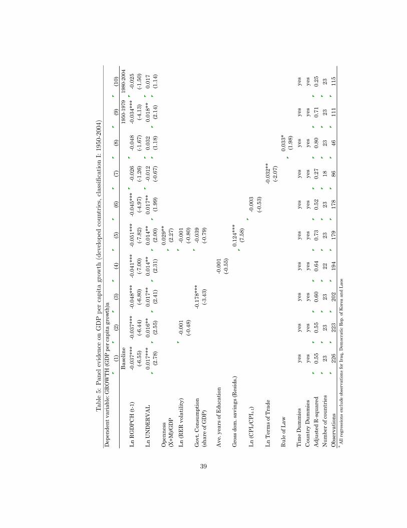
Table5:PanelevidenceonGDPpercapitagrowth(developedcountries,classi�cationI:1950-2004)

(1)

(2)

(3)

(4)

(5)

(6)

(7)

(8)

(9)

(10)

Bas

elin

e19

50­1

979

1980

­200

4Ln

 RG

DPC

H (t

­1)

­0.0

37**

*­0

.037

***

­0.0

48**

*­0

.041

***

­0.0

51**

*­0

.045

***

­0.0

26­0

.048

­0.0

34**

*­0

.025

(­6.5

5)(­6

.44)

(­6.8

0)(­7

.00)

(­7.8

2)(­4

.97)

(­1.2

6)(­1

.67)

(­4.1

3)(­1

.50)

Ln U

ND

ER

VA

L0.

017*

**0.

016*

*0.

017*

*0.

014*

*0.

014*

*0.

017*

*­0

.012

0.03

20.

018*

*0.

017

(2.7

8)(2

.55)

(2.4

1)(2

.31)

(2.0

0)(1

.99)

(­0.6

7)(1

.18)

(2.1

4)(1

.14)

Ope

nnes

s0.

029*

*(X

+M)/G

DP

(2.2

7)

Ln (R

ER

 vol

atili

ty)

­0.0

01­0

.001

(­0.4

8)(­0

.80)

Gov

t. C

onsu

mpt

ion

­0.1

78**

*­0

.039

(sha

re o

f GD

P)(­3

.43)

(­0.7

9)

Ave

. yea

rs o

f Edu

catio

n­0

.001

(­0.5

5)G

ross

 dom

. sav

ings

 (Res

ids.)

0.12

4***

(7.5

8)Ln

 (CPI

t/CPI

t­1)

­0.0

03(­0

.53)

Ln T

erm

s of T

rade

­0.0

32**

(­2.0

7)R

ule 

of L

aw0.

033*

(1.9

8)Ti

me 

Dum

mie

sye

sye

sye

sye

sye

sye

sye

sye

sye

sye

sC

ount

ry D

umm

ies

yes

yes

yes

yes

yes

yes

yes

yes

yes

yes

Adj

uste

d R

­squ

ared

0.55

0.55

0.60

0.64

0.73

0.52

0.27

0.80

0.71

0.25

Num

ber o

f cou

ntri

es23

2323

2223

2318

2323

23O

bser

vatio

ns22

622

320

219

417

917

886

4611

111

5a  A

ll re

gres

sion

s ex

clud

e ob

serv

atio

ns fo

r Ir

aq, D

emoc

ratic

 Rep

. of K

orea

 and

 Lao

s

Dep

ende

nt v

aria

ble:

 GR

OW

TH (G

DP 

per c

apita

 gro

wth)

a

39

Table6:Panelevidenceoninvestmentgrowth(allcountries:1960-2004)

(1)

(2)

(3)

(4)

(5)

(6)

(7)

(8)

Base

line

Ln R

GD

PCH

t­1­0

.071

***

­0.0

70**

*­0

.087

***

­0.0

97**

*­0

.110

***

­0.1

10**

*­0

.162

**­0

.080

***

(­5.6

5)(­4

.90)

(­5.9

6)(­6

.49)

(­5.8

1)(­5

.09)

(­2.2

9)(­6

.36)

Ln U

ND

ERVA

L t­0

.006

­0.0

02­0

.013

­0.0

14­0

.017

­0.0

090.

040

0.10

7***

(­0.5

1)(­0

.12)

(­0.9

9)(­1

.08)

(­1.1

9)(­0

.49)

(0.7

8)(3

.30)

Ln U

ND

ERVA

L  t­1

0.04

4***

0.04

2***

0.04

2***

0.04

2***

0.05

1***

0.02

90.

003

0.15

3***

(3.2

4)(2

.94)

(3.0

0)(3

.00)

(3.4

2)(1

.64)

(0.0

8)(4

.80)

Ln U

ND

ERVA

Lt­

2­0

.015

­0.0

25**

­0.0

21*

­0.0

23*

­0.0

27*

­0.0

220.

034

0.10

1***

(­1.2

7)(­2

.12)

(­1.8

1)(­1

.94)

(­1.9

3)(­1

.38)

(1.1

8)(3

.09)

Gov

ernm

ent C

onsu

mpt

ion

0.14

10.

148

0.22

4**

0.29

5**

0.18

10.

299

(sha

re o

f GD

P)(1

.41)

(1.5

1)(2

.21)

(2.5

5)(1

.32)

(0.9

4)Ln

 (CPI

t/CPI

t­1)

­0.0

10**

*­0

.009

***

­0.0

09**

*­0

.008

***

­0.0

07**

0.01

6(­3

.88)

(­3.6

1)(­3

.58)

(­2.7

0)(­2

.50)

(0.7

9)Ln

 (RER

 vol

atili

ty)

­0.0

09**

­0.0

09**

­0.0

09**

­0.0

11**

*­0

.015

***

0.00

3(­2

.53)

(­2.5

7)(­2

.55)

(­2.9

0)(­3

.10)

(0.3

4)O

penn

ess

0.08

4***

0.07

7***

0.10

1***

0.04

8*0.

019

(Exp

orts

+Im

port

s as

 sha

re o

f GD

P)(4

.31)

(3.9

1)(3

.79)

(1.8

2)(0

.32)

Gro

ss D

omes

tic 

Savi

ng (R

esid

uals

)0.

137*

**0.

202*

**0.

166*

*­0

.010

(2.8

1)(3

.57)

(2.3

1)(­0

.06)

Aver

age 

year

s of

 Edu

catio

n­0

.005

(­0.7

5)

Ln T

erm

s of

 Tra

de­0

.019

(­0.9

8)Ru

le o

f Law

0.07

0**

(2.5

8)

Ln(R

GD

PCH

)x(L

nUN

Dt+

LnU

ND

t­1+L

nUN

Dt­

2)­0

.013

***

(­3.8

2)Ti

me 

Dum

mie

sye

sye

sye

sye

sye

sye

sye

sye

sC

ount

ry D

umm

ies

yes

yes

yes

yes

yes

yes

yes

yes

LnU

ND

t+ L

nUN

Dt­

1 + L

nUN

Dt­2

0.02

30.

015

0.00

80.

005

0.00

7­0

.002

0.07

7­

Wal

d st

atis

tic3.

196

1.23

80.

335

0.14

10.

187

0.00

51.

045

­p­

valu

e(0

.074

)(0

.266

)(0

.563

)(0

.708

)(0

.666

)(0

.942

)(0

.307

)­

Adju

sted

 R­s

quar

ed0.

180.

220.

250.

260.

330.

190.

220.

200.

19N

umbe

r of c

ount

ries

153

138

138

138

9010

213

115

3O

bser

vati

ons

712

639

639

639

432

395

234

712

a  All 

regr

essi

ons 

excl

ude 

obse

rvat

ions

 for 

whi

ch L

n(U

ND

ER

VA

L)<­

1.5 

and 

Ln(U

ND

ER

VAL)

>1.5

Dep

ende

nt v

aria

ble:

 GRO

WTH

GFC

F (I

nves

tmen

t gro

wth

)a

40

Table7:Panelevidenceoninvestmentgrowth(developingcountries,classi�cationI:1960-2004)

(1)

(2)

(3)

(4)

(5)

(6)

(7)

(8)

(9)

Bas

elin

e19

60­1

984

1985

­200

4Ln

 RG

DPC

Ht­1

­0.0

83**

*­0

.081

***

­0.1

13**

*­0

.124

***

­0.1

34**

*­0

.156

***

­0.1

81**

­0.1

68**

*­0

.127

***

(­5.8

8)(­5

.01)

(­5.8

8)(­6

.27)

(­5.1

7)(­5

.37)

(­2.0

9)(­3

.01)

(­5.5

5)Ln

 UN

DE

RV

AL t

0.01

20.

017

0.02

7*0.

026

0.03

6*0.

015

0.04

00.

019

­0.0

01(0

.86)

(1.1

4)(1

.70)

(1.6

3)(1

.69)

(0.8

1)(0

.68)

(0.5

3)(­0

.06)

Ln U

ND

ER

VA

L t­1

0.04

8***

0.04

0**

0.03

2*0.

032*

*0.

023

0.04

8**

­0.0

220.

092*

*0.

049*

**(3

.18)

(2.4

7)(1

.96)

(1.9

7)(1

.17)

(2.5

0)(­0

.49)

(2.1

3)(2

.93)

Ln U

ND

ER

VA

L t­2

0.00

60.

003

0.00

1­0

.000

­0.0

03­0

.004

0.02

80.

008

0.00

8(0

.47)

(0.2

0)(0

.04)

(­0.0

2)(­0

.15)

(­0.2

2)(0

.76)

(0.1

7)(0

.052

)G

over

nmen

t Con

sum

ptio

n0.

024

0.09

20.

149

0.14

90.

319*

*0.

211

(sha

re o

f GD

P)(0

.21)

(0.7

6)(1

.20)

(0.9

8)(2

.09)

(0.5

7)Ln

 (CPI

t/CPI

t­1)

­0.0

10**

*­0

.007

***

­0.0

07**

*­0

.007

**­0

.006

0.02

3(­3

.59)

(­2.6

1)(­2

.63)

(­2.0

8)(­1

.61)

(0.9

6)Ln

 (RE

R v

olat

ility

)­0

.015

***

­0.0

11**

­0.0

11**

­0.0

15**

­0.0

12**

­0.0

05(­3

.30)

(­2.3

9)(­2

.38)

(­2.5

2)(­2

.04)

(­0.5

2)O

penn

ess

0.06

5***

0.06

0**

0.04

90.

101*

**0.

030

(Exp

orts

+Im

port

s as

 sha

re o

f GD

P)(2

.63)

(2.4

2)(1

.60)

(2.8

4)(0

.39)

Ext

erna

l Deb

t­0

.051

***

­0.0

50**

*­0

.054

***

­0.0

43**

­0.0

07(s

hare

 of G

NI)

(­3.8

7)(­3

.83)

(­3.4

3)(­2

.53)

(­0.1

7)G

ross

 Dom

esti

c Sa

ving

 (Res

idua

ls)

0.13

6**

0.12

60.

227*

**0.

084

(2.1

6)(1

.55)

(2.7

8)(0

.43)

Ln T

erm

s of

 Tra

de­0

.015

(­0.7

1)A

vera

ge y

ears

 of E

duca

tion

0.00

2(0

.17)

Rule

 of L

aw0.

087*

*(2

.61)

Tim

e D

umm

ies

yes

yes

yes

yes

yes

yes

yes

yes

yes

Cou

ntry

 Dum

mie

sye

sye

sye

sye

sye

sye

sye

sye

sye

sLn

UN

Dt+

 LnU

ND

t­1 +

 LnU

ND

t­20.

066

0.06

00.

060

0.05

80.

056

0.05

90.

046

0.11

80.

056

Wal

d st

atis

tic15

.79

10.9

48.

858.

373.

864.

800.

274.

904.

43p­

valu

e(0

.000

)(0

.001

)(0

.003

)(0

.004

)(0

.049

)(0

.029

)(0

.600

)(0

.027

)(0

.035

)A

djus

ted 

R­s

quar

ed0.

230.

280.

320.

330.

240.

370.

230.

450.

22N

umbe

r of

 cou

ntri

es13

011

510

010

076

6198

6513

0O

bser

vati

ons

552

484

420

420

294

261

173

166

386

a  All 

regr

essi

ons 

excl

ude 

obse

rvat

ions

 for w

hich

 Ln(

UN

DE

RV

AL)

<­1.

5 an

d Ln

(UN

DE

RV

AL)

>1.5

Dep

ende

nt v

aria

ble:

 GR

OW

THG

FCF 

(Inv

estm

ent g

row

th)a

41

Table8:Panelevidenceoninvestmentgrowth(developedcountries,classi�cationI:1960-2004)

(1)

(2)

(3)

(4)

(5)

(6)

(7)

(8)

(9)

(10)

Base

line

Ln R

GD

PCH

t­1­0

.109

***

­0.1

07**

*­0

.119

***

­0.1

25**

*­0

.107

***

­0.1

04**

*­0

.116

***

­0.1

21**

*­0

.147

***

­0.0

98*

(­4.4

8)(­4

.44)

(­5.3

8)(­5

.32)

(­4.3

4)(­4

.29)

(­5.0

0)(­5

.49)

(­5.0

2)(­1

.79)

Ln U

ND

ERVA

L t­0

.019

­0.0

24­0

.033

­0.0

49*

­0.0

17­0

.011

­0.0

42­0

.043

­0.0

33­0

.092

(­0.6

3)(­0

.81)

(­1.2

2)(­1

.68)

(­0.5

5)(­0

.37)

(­1.4

6)(­1

.57)

(­1.0

9)(­1

.77)

Ln U

ND

ERVA

L t­1

0.05

6*0.

043

0.05

0*0.

064*

*0.

057*

0.05

8*0.

055*

0.05

4*0.

053

0.07

1(1

.72)

(1.3

0)(1

.69)

(2.0

6)(1

.70)

(1.7

8)(1

.77)

(1.8

2)(1

.58)

(1.5

0)Ln

 UN

DER

VAL t

­2­0

.020

­0.0

120.

006

­0.0

10­0

.025

­0.0

23­0

.007

0.00

7­0

.018

­0.0

39(­0

.81)

(­0.4

8)(0

.28)

(­0.4

2)(­0

.93)

(­0.9

1)(­0

.28)

(0.3

0)(­0

.72)

(0.9

0)G

over

nmen

t Con

sum

ptio

n­0

.283

*­0

.251

*­0

.085

(sha

re o

f GD

P)(­1

.91)

(­1.7

0)(­0

.58)

Gro

ss D

omes

tic S

avin

g (R

esid

uals

)0.

233*

**0.

177*

**(5

.38)

(3.7

1)O

penn

ess

0.08

7***

0.08

1***

0.05

4**

(Exp

orts

+Im

port

s as

 sha

re o

f GD

P)(3

.82)

(3.5

2)(2

.36)

Ln (R

ER v

olat

ility

)­0

.006

(­1.3

1)Ln

 (CPI

t/CPI

t­1)

­0.0

21­0

.029

**­0

.020

(­1.5

3)(­2

.23)

(­1.5

8)Av

erag

e ye

ars 

of E

duca

tion

­0.0

08(­1

.52)

Ln T

erm

s of

 Tra

de­0

.058

(­1.3

7)Ru

le o

f Law

Tim

e D

umm

ies

yes

yes

yes

yes

yes

yes

yes

yes

yes

yes

Coun

try 

Dum

mie

sye

sye

sye

sye

sye

sye

sye

sye

sye

sye

sLn

UN

Dt+

 LnU

ND

t­1 +

 LnU

ND

t­20.

017

0.00

70.

023

0.00

50.

015

0.02

40.

007

0.01

80.

002

­0.0

60W

ald 

stat

istic

0.61

0.11

1.41

0.05

0.46

1.19

0.10

0.79

0.00

11.

09p­

valu

e(0

.436

)(0

.744

)(0

.236

)(0

.826

)(0

.497

)(0

.275

)(0

.749

)(0

.374

)(0

.940

)(0

.296

)Ad

just

ed R

­squ

ared

0.32

0.34

0.45

0.39

0.32

0.34

0.42

0.48

0.43

0.10

Num

ber 

of co

untr

ies

2323

2323

2323

2323

2218

Obs

erva

tions

160

160

160

160

158

157

157

157

130

86a  A

ll re

gres

sion

s ex

clud

e ob

serv

atio

ns fo

r w

hich

 Ln(

UN

DE

RV

AL)

<­1.

5 an

d Ln

(UN

DE

RVA

L)>1

.5

Dep

ende

nt v

aria

ble:

 GRO

WTH

GFC

F (I

nves

tmen

t gro

wth

)a

42

Table9:DynamicPanelEstimationoftheinvestmentgrowthe¤ectsofundervaluation

Clas

sif I

Clas

sif I

IC

lass

if I

Clas

sif I

I(1

)(2

)(3

)(4

)(5

)(a

) Lag

ged 

inve

stm

ent g

row

th0.

213*

**0.

003

­0.0

050.

216*

**0.

234*

**(4

.34)

(0.0

4)(­0

.07)

(4.0

9)(4

.52)

(b) L

n in

tial

 inco

me

­0.0

80**

*­0

.131

***

­0.1

11**

*­0

.089

***

­0.0

83**

*(­6

.25)

(­3.6

6)(­3

.12)

(­6.4

1)(­6

.09)

(c) L

n U

ND

ERVA

L t0.

010

­0.0

05­0

.102

**0.

021*

0.01

9(0

.83)

(­0.1

4)(­2

.12)

(1.6

6)(1

.53)

(d) L

n U

ND

ERVA

L t­1

0.03

1***

0.04

80.

097*

*0.

042*

**0.

033*

*(2

.69)

(1.6

4)(2

.52)

(2.7

1)(2

.32)

(e) =

 [(c)

+(d)

]/[1­

(a)]

0.05

20.

045

­0.0

040.

079

0.06

7W

ald 

stat

istic

13.9

22.

430.

0217

.42

12.8

3p­

valu

e(0

.000

)(0

.119

)(0

.890

)(0

.000

)(0

.000

)Ti

me 

dum

mie

sye

sye

sye

sye

sye

sN

o. o

f cou

ntri

es11

523

2392

96O

bser

vatio

ns45

211

510

333

734

9In

stru

men

t  ra

nk30

2323

3030

J­st

atis

tic23

.79

15.5

015

.55

23.0

521

.10

Sarg

an T

est (

p­va

lue)

0.25

20.

277

0.27

40.

286

0.39

1

All

coun

trie

sD

evel

oped

 Cou

ntri

esD

evel

opin

g Co

untr

ies

a Res

ults

 obt

aine

d us

ing 

the 

orth

ogon

al d

evia

tion

s tr

ansf

orm

atio

n an

d as

sum

ing 

exog

enei

ty o

f tim

e du

mm

ies.

 All

regr

essi

ons 

excl

ude 

obse

rvat

ions

 for 

whi

ch L

n(U

ND

ER

VA

L)<­

1.5 

and 

Ln(U

ND

ERV

AL)

>1.5

Dep

ende

nt v

aria

ble:

 GRO

WTH

GFC

F (I

nves

tmen

t gro

wth

)a

43

Table10:Panelevidenceoninvestmentgrowth,testingforoutliersandasymmetries

(1)

(2)

(3)

(4)

(5)

Bas

elin

e­1

.5<L

nUN

D<1

.5­1

.0<L

nUN

D<1

.0­0

.5<L

nUN

D<0

.5Ln

UN

D>0

LnU

ND

<0Ln

 RG

DPC

Ht­

1­0

.083

***

­0.0

82**

*­0

.098

***

­0.0

83**

*­0

.119

***

(­5.8

8)(­5

.70)

(­6.3

7)(­4

.12)

(­3.5

3)Ln

 UN

DER

VAL t

0.01

20.

008

­0.0

26­0

.049

*0.

053

(0.8

6)(0

.54)

(­1.2

6)(­1

.90)

(1.6

4)Ln

 UN

DER

VAL t

­10.

048*

**0.

045*

**0.

078*

**0.

066*

**0.

030

(3.1

8)(2

.92)

(4.4

0)(3

.38)

(1.1

0)Ln

 UN

DER

VAL t

­20.

006

0.00

80.

011

0.02

6­0

.012

(0.4

7)(0

.61)

(0.7

5)(1

.31)

(­0.4

9)Ti

me 

Dum

mie

sye

sye

sye

sye

sye

sCo

untr

y D

umm

ies

yes

yes

yes

yes

yes

LnU

ND

t+ L

nUN

Dt­1

 + L

nUN

Dt­

20.

066

0.06

10.

063

0.04

30.

072

Wal

d st

atis

tic15

.79

12.8

28.

332.

192.

81p­

valu

e(0

.000

)(0

.000

)(0

.004

)(0

.139

)(0

.094

)Ad

just

ed R

­squ

ared

0.23

0.22

0.23

0.40

0.03

7N

umbe

r of

 coun

trie

s13

012

611

310

485

Obs

erva

tion

s55

254

046

332

722

5

Dep

ende

nt v

aria

ble:

 GRO

WTH

GFC

F (In

vest

men

t gro

wth

)

44