department of civil and environmental engineering date:

Experimental Investigation of Thermodynamic and Kinetic Properties of Semi-volatile

Organic Aerosols

by

Rawad Saleh

Department of Civil and Environmental Engineering

Duke University

Date:_______________________

Approved:

___________________________

Andrey Khlystov, Supervisor

___________________________

Ana Barros

___________________________

Prakash Bhave

___________________________

Claudia Gunsch

___________________________

Alan Shihadeh

Dissertation submitted in partial fulfillment of

the requirements for the degree of Doctor of Philosophy in the Department of

Civil and Environmental Engineering in the Graduate School

of Duke University

2010

ABSTRACT

Experimental Determination of Thermodynamic and Kinetic Properties of Semi-volatile

Organic Aerosols

by

Rawad Saleh

Department of Civil and Environmental Engineering

Duke University

Date:_______________________

Approved:

___________________________

Andrey Khlystov, Supervisor

___________________________

Ana Barros

___________________________

Prakash Bhave

___________________________

Claudia Gunsch

___________________________

Alan Shihadeh

An abstract of a dissertation submitted in partial

fulfillment of the requirements for the degree

of Doctor of Philosophy in the Department of

Civil and Environmental Engineering in the Graduate School

of Duke University

2010

Copyright by

Rawad Saleh

2010

iv

Abstract

We have developed and applied novel experimental techniques for

determination of thermodynamic and kinetic properties of semi-volatile organic

aerosols. The thermodynamic properties investigated were the saturation pressure (Psat),

enthalpy of vaporization (∆H) and activity coefficient (γ), and the kinetic property was

the evaporation coefficient (α).

The thermodynamic properties were determined using the integrated volume

method (IVM), which relies on measurements of aerosol particle concentrations at

different thermodynamic equilibrium states. The measured decrease in particle

concentration upon heating in a flow tube, a thermodenuder, can be correlated with Psat

and ∆H via the IVM equation, which was derived from fundamental principles, namely

the Clausius-Clapeyron relation, mass conservation, and ideal gas law. The main

advantage of the IVM over other methods reported in the literature is that the other

methods use kinetic-based techniques to measure thermodynamic properties which

require assumptions on the usually unknown evaporation coefficient; the IVM, on the

other hand, is equilibrium-based and thus requires no assumption on the evaporation

coefficient. We have applied the IVM to C-4, -6, -7, and -9 dicarboxylic acid aerosols,

which are pertinent to atmospheric secondary organic aerosols. Psat and ∆H values

v

obtained for these compounds were respectively 3.7×10-4 Pa and 88 kJ/mol, 3.4 ×10-5 Pa

and 135 kJ/mol, 7.2×10-5 Pa and 149 kJ/mol, and 1.4 ×10-5 Pa and 145 kJ/mol.

The IVM was also used to determine activity coefficients of individual

compounds in binary mixtures as a function of their mole fractions. We demonstrated

this method using the following four model systems. System 1: adipic acid – pimelic

acid, which illustrated polar organic – polar organic interactions. Non-ideal behavior

was observed with activity coefficients of approximately three at infinite dilution.

System 2: adipic acid – dioctyl sebacate, which illustrated polar organic – non-polar

organic interactions. The compounds in this experiment did not form a solution. System

3: adipic acid – ammonium sulfate, which illustrates polar organic – inorganic

interactions. The compounds in this experiment did not form a solution. System 4:

adipic acid – ambient extracts, which illustrated the potential use of the method to study

partitioning behavior of individual components in a complex matrix approximating that

of real ambient aerosol. The measured activity coefficient of adipic acid was less than

unity for the tested range of mixing ratios, indicating suppression of volatility of this

compound in ambient organic matrix.

We have investigated three controversial issues associated with the IVM as well

as other methods which utilize thermodenuders and/or aerosol generation by spray

atomization and drying: 1) equilibration time scales in thermodenuders, 2) the need for

an activated carbon (AC) denuder in the cooling section, and 3) the effect of residual

vi

solvent on measured thermodynamic properties of aerosols generated by spray

atomization and drying. Both numerical simulations and experiments showed that the

aerosols approached equilibrium within reasonable residence times (15 s – 30 s) for

aerosol size distributions typical for laboratory measurements. We have also performed

dimensional analysis on the problem of equilibration in TDs, and derived a

dimensionless equilibration parameter which can be used to determine the residence

time needed for an aerosol of given sized distribution and kinetic properties to approach

equilibrium. Using both model simulations and experiments, we have shown that with

aerosol size distributions relevant to both ambient and laboratory measurements re-

condensation in the cooling section, with and without an AC denuder, was negligible.

Thus, there is no significant benefit in using an AC denuder in the cooling section. To

investigate the effect of residual solvent on measured thermodynamic properties, we

compared measurements of Psat and ∆H of C-6 (adipic) and C-9 (azelaic) dicarboxylic

acid aerosols generated by atomization of aqueous solutions to those generated by

homogeneous condensation using a modified Sinclair - La Mer generator. We found no

statistically significant difference between the tested aerosol generation methods,

indicating that residual solvent carried by the particles had no impact on the

measurements.

To determine the evaporation coefficient, we developed the integrated volume –

tandem differential mobility analysis (IV-TDMA) method. This thermodenuder-based

vii

method allows separate determination of the three parameters governing aerosol

evaporation, namely, Psat, surface free energy (σ), and α. Psat was determined using the

IVM, while α and σ were determined by fitting particle evaporation rates measured

under non-equilibrium conditions to a numerical model of the evaporation process. α

was determined in a size range where surface free energy effects were negligible,

allowing for single parameter optimization. We obtained α and σ values of 0.07 and 0.15

J/m2, 0.08 and 0.17 J/m2 and 0.24 and 0.23 J/m2 for C-4, -6, and -7 dicarboxylic acids,

respectively.

viii

Contents

Abstract ......................................................................................................................................... iv

List of Tables ................................................................................................................................ xii

List of Figures ............................................................................................................................ xiii

Acknowledgements ...................................................................................................................xvi

1. Introduction ............................................................................................................................... 1

1.1 Motivation and significance ............................................................................................ 1

1.2 The state of the art and the scientific gaps .................................................................... 4

1.2.1 Techniques used to determine Psat and ∆H of semi-volatile organic aerosols .... 4

1.2.2 Techniques used to determine activity coefficients (γ) .......................................... 5

1.2.3 Aerosol generation and the effect of residual solvent ............................................ 7

1.2.4 Thermodenuders ......................................................................................................... 8

1.2.5 The evaporation coefficient ........................................................................................ 9

1.3 Objectives ......................................................................................................................... 11

1.4 Research hypotheses and chapter flow ....................................................................... 12

2. Determination of saturation pressure and enthalpy of vaporization of semi-volatile

aerosols ......................................................................................................................................... 14

2.1 The integrated volume method (IVM) ........................................................................ 14

2.2 Experimental section ...................................................................................................... 16

2.2.1 Aerosol generator ...................................................................................................... 16

2.2.2 The thermodenuder .................................................................................................. 17

2.2.3 The sizing system ...................................................................................................... 18

ix

2.2.4 Experimental procedure ........................................................................................... 19

2.3 Results and discussion ................................................................................................... 20

2.3.1 Psat and ∆H .................................................................................................................. 20

2.3.2 Issues of special consideration regarding the IVM ............................................... 23

3. Determination of activity coefficients of binary mixtures ................................................. 25

3.1 Experimental section ...................................................................................................... 25

3.1.1 Experimental setup and procedure......................................................................... 25

3.1.2 Sample preparation ................................................................................................... 26

3.2 Theory and data analysis ............................................................................................... 27

3.2.1 Extension of the IVM to multi-component aerosols ............................................. 27

3.2.2 Algorithm to calculate activity coefficients ........................................................... 29

3.2.2.1 Mole fraction calculation ................................................................................... 29

3.2.2.2 Activity coefficients ........................................................................................... 30

3.2.2.3 Estimation of molecular weight of organic components in ambient extracts

.......................................................................................................................................... 31

3.2.2.4 Uncertainty analysis .......................................................................................... 32


3.3.1 Adipic acid – pimelic acid ........................................................................................ 33

3.3.2 Adipic acid – dioctyl sebacate and adipic acid – ammonium sulfate ................ 39

3.3.3 Adipic acid – ambient extracts ................................................................................ 42

3.4 Conclusions ..................................................................................................................... 46

4. Effect of aerosol generation method on measured thermodynamic properties ............ 48

x

4.1 Methods ........................................................................................................................... 48

4.1.1 Aerosol generation .................................................................................................... 49

4.1.2 Aerosol sizing and conditioning ............................................................................. 52

4.1.3 The integrated volume method ............................................................................... 53

4.1.4 SEM imaging .............................................................................................................. 54


4.2.1 Saturation pressures and enthalpies of vaporization ........................................... 55

4.2.2 SEM images ................................................................................................................ 59

4.3 Conclusions ..................................................................................................................... 62

5. On transport phenomena and equilibration time scales in thermodenuders ................ 63

5.1 Introduction ..................................................................................................................... 63

5.2 Theory .............................................................................................................................. 66

5.2.1 Plug flow formulation ................................................................................................. 68

5.2.2 The equilibration parameter (tr / τ) ......................................................................... 70

5.2.3 Re-condensation in the cooling section .................................................................. 73

5.3 Experimental ................................................................................................................... 73

5.4 Reuslts and discussion ................................................................................................... 77

5.4.1 Effect of particle size distribution ........................................................................... 77

5.4.2 Effect of the evaporation coefficient ....................................................................... 78

5.4.3 Effect of thermodynamic properties and mixture complexity ............................ 80

5.4.4 Effect of the equilibration parameter ...................................................................... 83

5.4.5 Re-condensation in the cooling section .................................................................. 87

xi

5.4.6 TD design guidelines ................................................................................................ 91

5.5 Conclusions ..................................................................................................................... 92

6. Determination of evaporation coefficients of semi-volatile organic aerosols ................ 95

6.1 Introduction ..................................................................................................................... 95

6.2 The IV-TDMA method ................................................................................................... 99

6.2.1 The IVM .................................................................................................................... 100

6.2.2 The TDMA method ................................................................................................. 101

6.3 Experimental section .................................................................................................... 104

6.3.1 Experimental setup and procedure....................................................................... 104

6.3.2 Uncertainty analysis ................................................................................................ 108

6.4 Results and discussion ................................................................................................. 109

6.4.1 Evaporation coefficients and surface free energies ............................................ 109

6.4.2 Temperature dependence of the evaporation coefficient .................................. 114

6.5 Conclusions ................................................................................................................... 116

7. Conclusions ............................................................................................................................ 118

References .................................................................................................................................. 121

Biography ................................................................................................................................... 132

xii

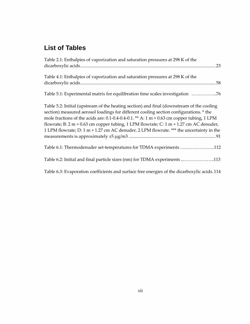
List of Tables

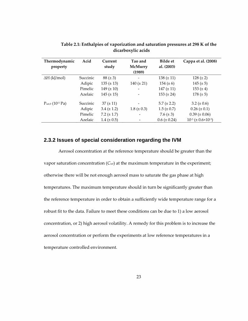
Table 2.1: Enthalpies of vaporization and saturation pressures at 298 K of the

dicarboxylic acids ........................................................................................................................ 23


dicarboxylic acids ........................................................................................................................ 58

Table 5.1: Experimental matrix for equilibration time scales investigation ……………..76

Table 5.2: Initial (upstream of the heating section) and final (downstream of the cooling

section) measured aerosol loadings for different cooling section configurations. * the

mole fractions of the acids are: 0.1-0.4-0.4-0.1. ** A: 1 m × 0.63 cm copper tubing, 1 LPM

flowrate; B: 2 m × 0.63 cm copper tubing, 1 LPM flowrate; C: 1 m × 1.27 cm AC denuder,

1 LPM flowrate; D: 1 m × 1.27 cm AC denuder, 2 LPM flowrate. *** the uncertainty in the

measurements is approximately ±5 μg/m3 ............................................................................. 91

Table 6.1: Thermodenuder set-temperatures for TDMA experiments …………………..112

Table 6.2: Initial and final particle sizes (nm) for TDMA experiments ...………………..113

Table 6.3: Evaporation coefficients and surface free energies of the dicarboxylic acids . 114

xiii

List of Figures

Figure 2.1: IVM experimental setup ......................................................................................... 18

Figure 2.2: IVM measurements. Triangles: succinic acid; diamonds: adipic acid; stars:

pimelic acid; circles: azelaic acid. Solid lines are 2-parameter fits based on equation 2.6 22

Figure 3.1-a: Change in total aerosol volume for aidpic acid – pimelic acid mixtures

between 25 ⁰C and 35 ⁰C. The solid line is the fit based on the model described in section

3.2.1. The dotted lines are uncertainty envelopes, based on the analysis in section 3.2.2.4

....................................................................................................................................................... 35

Figure 3.1-b: Activity coefficients for adipic acid and pimelic acid when present in a

binary solution, based on the model described in section 3.2.2. The dotted lines are

uncertainty envelopes, based on the analysis in section 3.2.2.4 ........................................... 36

Figure 3.2: Change in total aerosol volume for aidpic acid – dioctyl sebacate mixtures

between 25 ⁰C and 35 ⁰C. ............................................................................................................ 40

Figure 3.3: Change in total aerosol volume for aidpic acid – ammonium sulfate mixtures

between 25 ⁰C and 35 ⁰C. ............................................................................................................ 41

Figure 3.4-a: Change in total aerosol volume for aidpic acid – ambient extracts mixtures

between 25 ⁰C and 35 ⁰C. The solid line is the fit based on the model described in section

3.2.2. The dotted lines are uncertainty envelopes, based on the analysis in section 3.2.2.4.

The volume change of the pure ambient extract (0.7 μm3/cm3) is not shown, but was

taken into account when calculating the fit and the uncertainty envelopes. ..................... 43

Figure 3.4-b: Activity coefficients for adipic acid when present in a solution with

ambient extracts, based on the model described in section 3.2.2. The dotted lines are

uncertainty envelopes, based on the analysis in section 3.2.2.4.. ......................................... 44

Figure 4.1: Schematic of IVM experimental setup. For homogeneous condensation, the 6-

jet atomizer is replaced with a CMAG, and the diffusion dryer is removed ..................... 51

Figure 4.2: Measured change in total volume concentration of adipic acid (a) and azelaic

acid (b) aerosol particles versus inverse of set-temperature ................................................. 57

Figure 4.3: SEM images for (a) adipic acid generated by homogeneous condensation, (b)

adipic acid generated by atomization, (c) azelaic acid generated by homogeneous

condensation, and (d) azelaic acid generated by atomization .............................................. 62

xiv

Figure 5.1: Experimental setup.................................................................................................. 76

Figure 5.2: Measured and simulated particle mass change and dimensionless vapor

build-up profiles for adipic acid aerosol in a TD. Tin = 25 ⁰C and Tw = 40 ⁰C. Squares &

solid: C0 = 390 μg/m3, Ntot = 1012 particles/m3, dp,cs = 65 nm; diamonds & broken: C0 = 245

μg/m3, Ntot = 6×1011 particles/m3, dp,cs = 65 nm; stars & dotted: C0 = 68 μg/m3, Ntot = 2.5×1011

particles/m3, dp,cs = 60 nm ............................................................................................................ 79

Figure 5.3: Measured and simulated vapor build-up profiles for adipic acid aerosol (C0 =

390 μg/m3, Ntot = 1012 particles/m3, dp,cs = 65 nm) in a TD. The simulations were performed

with α as a variable parameter as indicated in the Figure. Tin = 25 ⁰C and Tw = 40 ⁰C. ...... 80

Figure 5.4: Measured and simulated vapor build-up profiles. Squares & solid: adipic

acid, C0 = 390 μg/m3 and dcs = 65 nm; triangles & broken: pimelic acid, C0 = 307 μg/m3 and

dcs = 67 nm; circles & dotted: succinic+adipic+pimelic+azelaic acid mixture, C0 = 313

μg/m3 and dcs = 61 nm. Tin = 25 ⁰C and Tw = 40 ⁰C. ................................................................... 83

Figure 5.5: Vapor build up as a function of the equilibration parameter for the

measurements in Figure 5.2 and Figure 5.4. All the simulations in Figure 5.2 and Figure

5.4 collapse on the solid line. Cg* = 1 corresponds to phase equilibrium at the TD

temperature .................................................................................................................................. 85

Figure 5.6: Simulated normalized vapor build-up profiles in a TD as a function of

residence time (bottom x-axis and left y-axis) and time-dependent equilibration

parameter (upper x-axis and right y-axis). T0 = 25 ⁰C; TTD = 40 ⁰C; ∆H = 100 kJ/mol; Co =

230 μg/m3; red: Csat = 0.14 μg/m3, ∆Csat/C0 = 5×10-4; green: Csat = 1.4 μg/m3, ∆Csat/C0 = 5×10-3;

blue: Csat = 14 μg/m3, ∆Csat/C0 = 0.05; cyan: Csat = 140 μg/m3, ∆Csat/C0 = 0.5; yellow: Csat = 225

μg/m3, ∆Csat/C0 = 0.8 ..................................................................................................................... 87

Figure 5.7: Maximum re-condensation fraction as a function of Cn .................................... 89

Figure 5.8: Maximum re-condensation fraction as a function of residence time in the

cooling section with and without an AC denuder for Cn = 0.5. Negative RF indicates net

evaporation of the aerosol relative to its state at the entrance of the heated TD. .............. 90

Figure 6.1: Relative importance of Fuchs-Sutugin correction (0 < Cm < 1 ) and Kelvin

effect (K > 1) for 100 nm – 600 nm particles at 298 K ............................................................ 102

Figure 6.2: TDMA experimental setup ................................................................................... 105

Figure 6.3: Residence time distribution in the thermodenuder .......................................... 106

xv

Figure 6.4: Change of particle size upon evaporation in TDMA experiments for (a)

succinic acid, (b) adipic acid, and (c) pimelic acid. Solid lines are theoretical fits based on

optimization of equation (6.2) to reproduce the observed size changes. Points on the

right side of the plots (larger diameters) are used for α determination, and points on the

left side (smaller diameters) are used for σ determination. ................................................ 111

Figure 6.5: Evaporation coefficients of the dicarboxylic acids as a function of

temperature. ............................................................................................................................... 116

xvi

Acknowledgements

It has been an honor to work with Prof Khlystov, whose scientific talent and

skills are unmatched. I learned something new in every single meeting we have had. To

say the least, I have been more than lucky to have Prof Khlystov as my PhD advisor.

I am grateful to my PhD committee members, Prof Barros, Dr Bhave, Prof

Gunsch, and Prof Shihadeh. I thank Dr Bhave for the valuable feedback and for

introducing me to the world of Air Quality Modeling. Prof Shihadeh’s contribution to

this dissertation was substantial, and being hosted in his aerosol lab every summer had

always been a fruitful and fun experience.

Many thanks to the people of Hudson basement and Annex for such an

enjoyable ride, especially to Andreas – we had a lot of good ones. The help of Ezzat,

Sarah, and Hassan made my “express missions” in the AUB aerosol lab doable; the

stress induced by time constraints was hugely overcome by the fun of working with you

guys.

Mom, dad, Roham, Ruba, and Saleh, your support during my PhD was a

continuation of your life-long support. Thanks for bearing with me through my grad

school years, while I could have made things much easier by going to work in Dubai

instead, like everybody does. Lynn, the dynamics you maintain brings about ultimate

happiness and comfort, which have materialized in all aspects of my life, including

graduate studentship.

1

1. Introduction

1.1 Motivation and significance

The importance of understanding ambient/atmospheric aerosols arises from the

extensive evidence of their effect on mankind in terms of health hazards and impact on

climate. Ambient aerosols have been associated with respiratory diseases (Koren and

O’Neill, 1998), cardiopulmonary diseases, cancer, and adverse reproductive effects

(Lewtas, 2007). Atmospheric aerosols can cause warming or cooling of the atmosphere

by absorbing or scattering light (Chung and Seinfeld, 2002; Maria et al., 2004). One of the

largest uncertainties on the Earth’s radiation budget is associated with the ability of

atmospheric aerosols to uptake water to form clouds (IPCC 4th assessment report, 2007).

Ambient aerosols are complex mixtures of organics, inorganics, and water

(Saxena and Hildemann, 1996; Ohta et al, 1990; Bardouki et al, 2002; Hueglen et al, 2004),

with organic compounds comprising up to 50% of the total mass concentration (Chow et

al., 1994; Murphy et al., 1998). Despite the substantial progress in the past few decades,

predictions of organic aerosol (OA) concentrations by local, regional and global air

quality models are still unable to fully reproduce ambient observations (Heald et al.,

2005; Vutkuru et al., 2006). One of the main uncertainties is associated with semi-volatile

OA, which constitutes a major fraction of both primary and secondary OA (Donahue et

al., 2006). Semi-volatile compounds constantly re-partition between the particle and the

2

gas phases as the temperature, relative humidity and concentrations of semi-volatile

species change with time (Turpin et al., 1991; Chow et al., 1994). Thus, understanding

the volatility of these organic species is of paramount importance for our ability to

predict OA concentrations (Fuzzi et al., 2006; Robinson et al., 2007). Volatility of semi-

volatile OA, or the extent to which they partition to the particulate phase, is a function of

their thermodynamic properties, namely, saturation pressure (Psat), enthalpy of

vaporization (∆H), and the activity coefficient (γ) with respect to the particulate phase

matrix.

OA is comprised of hundreds or sometimes thousands of compounds (Seinfeld

and Pandis, 1998), the thermodynamic properties of which are mostly unknown, which

makes individual representation of compounds in air quality models impossible.

Researchers have resorted to “lumping” compounds into groups with effective Psat and

∆H obtained from fits to yields of smog chamber experiments – controlled experiments

in which parent hydrocarbons are oxidized in the presence of ozone and UV light to

produce secondary organic aerosols (SOA) which simulate the reaction pathways that

occur in the atmosphere. One of the widely used models is the N.2P model of Odum et

al. (1997), where the compounds produced by each parent hydrocarbon are lumped into

two products, one with a low Psat and one with a high Psat, with ∆H assumed to be equal

for both. A newer approach is the volatility basis set (VBS) of Donahue et al. (2006). In

3

the VBS, semi-volatile organic compounds are lumped into fixed “volatility bins” with

decadal-spaced Psat values and decreasing ∆H with increasing Psat. The concentration in

each bin, or the “volatility distribution”, is obtained, again, from fits to smog chamber

yields. Pankow and Barsanti (2009) argued that the main limitation of the N.2P and VBS

is that the lumping of compounds is not based on fundamental molecular characteristics,

which puts the validity of extrapolation from smog chamber experimental conditions to

ambient conditions into question, especially due to the arbitrary assigned ∆H values.

Also, the lumping approaches do not allow the treatment of interaction between groups,

and thus the activity coefficients (γ) are assumed to be unity. Pankow and Barsanti

(2009) suggested a more fundamental approach to lump semi-volatile organic

compounds based on the number of carbon atoms and molecular polarity.

While the approach of Pankow and Barsanti (2009) is promising, the paucity of

data on thermodynamic properties of individual (or surrogate) semi-volatile organic

compounds hinders the progress in this direction. The reason is that standard bulk

measurement techniques used for volatile compounds cannot be applied to semi-volatile

compounds, and the new techniques developed for semi-volatiles over the past few

decades suffer from a variety of limitations, which has lead to results varying over 2-3

orders of magnitude (Clegg et al., 2008). Thus, there is a need for experimental

investigation of saturation pressures (Psat) and enthalpy of vaporizations (∆H) of semi-

4

volatile organic compounds pertinent to atmospheric OA, as well as activity coefficients

(γ) in the presence of other compounds.

It should be noted that the time scales of interest in air quality models are long

enough that phase change kinetics of semi-volatile OA – the time needed to achieve

equilibrium (re-partition between the particulate phase and the gas phase) in response to

a perturbation – is not relevant; the aerosol is assumed to be at equilibrium at each time

step. However, the time scales in laboratory and ambient measurements of

thermodynamic properties are comparable to those of phase change kinetics. The

knowledge of kinetic properties, namely the evaporation coefficient (α) is thus essential

for measurement interpretations.

1.2 The state of the art and the scientific gaps

1.2.1 Techniques used to determine Psat and ∆H of semi-volatile organic aerosols

There has been extensive work on estimating thermodynamic properties –

mainly saturation pressure (Psat) and enthalpy of vaporization (∆H) – of organic

compounds that pertain to semi-volatile OA. The most widely used method is the

Tandem Differential Mobility Analyzer (TDMA) (Rader and McMurry, 1986). In TDMA,

quasi-monodisperse aerosol is heated in a thermodenuder, a temperature controlled

flow tube, and the size change due to evaporation is measured. The observed particle

5

evaporation is compared to theoretical evaporation kinetics, from which Psat can be

estimated. Repeating the procedure at several different thermodenuder temperatures,

Psat(T) is obtained, and ∆H can be estimated using Clausius-Clapeyron relation. Another

technique is the temperature programmed thermal desorption (TPTD) (Chattopadhyay

and Ziemann, 2005; Cappa et al., 2007). In TPTD, aerosol is deposited in a temperature

controlled vacuum chamber. The evaporation rate is monitored using a mass

spectrometer, and Psat is estimated from comparison with the theoretical evaporation

rate given by the kinetic theory of gases. A recently developed technique is the Knudsen

Effusion Mass Spectrometer (KEMS) (Booth et al., 2009), where similar to TPTD, Psat is

obtained from comparing observed evaporation rates in a vacuum chamber to the

evaporation rate predicted by the kinetic theory of gases.

The major limitation of the methods briefly described above is that Psat, an

equilibrium property, is measured using non-equilibrium (kinetics-based) techniques.

This requires the assumption of ideal evaporation, which is mathematically represented

by an evaporation coefficient (α) equal to 1; this is not necessarily the case as outlined in

section 2.5. Thus, there is a need for developing an experimental technique that

decouples the effect of kinetics from measurements of Psat and ∆H; put in other words,

this technique needs to rely on equilibrium-based measurements.

1.2.2 Techniques used to determine activity coeffic ients ( γ)

6

In a multi-component solution, the vapor pressure of each component is

suppressed relative to Psat by the presence of other compounds according to Pv,i =xiγiPsat,i,

where xi is the mole fraction of component i in the solution and γi is the activity

coefficient. Most of the work reported in the literature has been on activity coefficients

of water in solution with organic compounds. There are two widely used techniques,

namely the Electrodynamic Balance (EDB) (Peng et al., 2001; Choi and Chen, 2002) and

the Hygroscopic Tandem Differential Mobility Analyzer (HTDMA) (Moore and

Raymond, 2008). In EDB, a single 5 μm – 40 μm droplet of aqueous solution is charged

then trapped and levitated in a temperature and humidity controlled chamber by

applying AC and DC fields. Relative change in mass at various controlled RH settings is

determined from the required DC voltage to balance the gravitational forces. Knowing

the concentration of the organic compound in the solution, γ can be obtained from

Kohler theory (RH = γxw), where xw is the mole fraction of water in the solution. Peng et

al. (2001) employed the EDB technique to obtain water activity in the presence of water

soluble organic compounds. The HTDMA is one of the variations of the tandem

differential mobility analyzer (TDMA) developed by Rader and McMurry (1986). Dry

quasi-monodisperse aerosol is sent to a reactor after mixing with a humidified air stream

to achieve a final RH; different RH values can be achieved by changing the mixing

ratios. Aerosol droplets grow due to water uptake to a final equilibrium size according

7

to Kohler theory, from which γ can be obtained. Moore and Raymond (2008) used the

HTDMA technique to estimate water activity present in solution with dicarboxylic acids.

The main limitation of the EDB and HTDMA methods is that the solute should be much

less volatile than the solvent, because it is assumed that only the solvent – water in this

case – undergoes partitioning with the gas phase. Thus, they can’t be used to determine

γ values of components with comparable Psat in organic mixtures.

The only experimental investigation of γ’s in organic-organic mixtures relevant

to atmospheric aerosol was reported by Cappa et al. (2008) using TPTD. γ values were

found to be less than unity for lower molecular mass dicarboxylic acids and larger than

unity for heavier dicarboxylic acids in an equi-molar mixture of C3-C10 and C12 di-

carboxylic acids. As mentioned in section 2.1, the TPTD suffers from the required

assumption of unity evaporation coefficient.

The paucity of data on γ’s of semi-volatile organic compounds hinders their

incorporation in air quality models, which may account for part of the uncertainty

(Pankow and Barsanti, 2009). This illustrates the importance of developing experimental

techniques that estimate γ’s of atmospheric-relevant semi-volatile organic compounds.

1.2.3 Aerosol generation and the effect of residual solvent

In all the aforementioned studies, organic aerosols were generated by

atomization of solutions – in water or alcohol – with subsequent stripping of the solvent

8

from the aerosol by diffusion (e.g. in a diffusion dryer or activated carbon denuder).

There has been evidence that part of the solvent can be retained in the aerosol (Cappa et

al. 2007 & 2008) when atomizing mono- and dicarboxylic acid solutions in water,

methanol, and 1-propanol. Cappa et al. (2007 & 2008) recommended preheating the

generated aerosol to evaporate the retained solvent. They reported an overestimation of

saturation pressure by up to a factor of 25, and underestimation of enthalpy of

vaporization by around 20% when the aerosol was not preheated. This was attributed to

1) contribution of retained solvent (which has greater Psat and lower ∆H than the

investigated compounds) to the evaporation flux in the Temperature Programmed

Desorption (TPD) experiments, and 2) the residual solvent molecules causing disruption

of the molecular structure at the surface of the organic aerosol, which enhanced

evaporation over the case of pure crystal structure. Since the vast majority of the Psat and

∆H values reported in the literature were obtained without pre-heating the aerosol, the

effect of remaining solvent on the volatility properties of organic substances needs to be

investigated.

1.2.4 Thermodenuders

Thermodenuders have been widely used in aerosol volatility studies, both in the

lab (e.g. An et al., 2007; Saleh et al., 2008; Fuallhaber et al., 2009) and in the field (e.g.

Wehner et al., 2004; Huffman et al., 2008; Dzepina et al., 2009). A thermodenuder is

9

simply a temperature controlled flow tube. When a volatile/semi-volatile aerosol is

heated as it flows through a thermodenuder, the aerosol particles respond by

evaporating. The extent to which the particles evaporate – the difference between initial

and final particle size distributions – gives information about their volatility.

There have been differences in configurations in the use of thermodenuders as

well as in interpretations of measurements, which has sometimes led to contradictory

conclusions. For example, Riipinen et al. (2010) concluded that equilibration time scales

in thermodenuders increase with increasing aerosol volatility, while Cappa (2010)

reached the very opposite conclusion. There is thus a need for theoretical and

experimental investigation of the technicalities of thermodenuders in order to provide a

solid foundation for proper use and data interpretation.

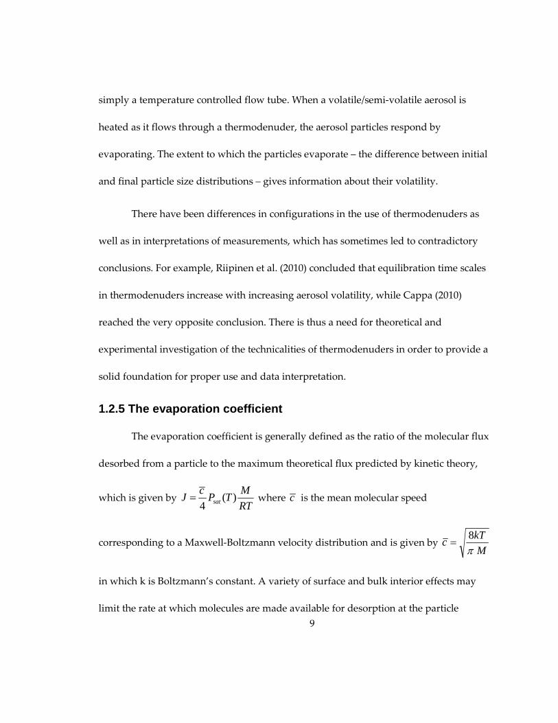
1.2.5 The evaporation coefficient

The evaporation coefficient is generally defined as the ratio of the molecular flux

desorbed from a particle to the maximum theoretical flux predicted by kinetic theory,

which is given by ( )4 sat

c MJ P T

RT= where c is the mean molecular speed

corresponding to a Maxwell-Boltzmann velocity distribution and is given by M

kTc

π8

=

in which k is Boltzmann’s constant. A variety of surface and bulk interior effects may

limit the rate at which molecules are made available for desorption at the particle

10

interface (Somorjai and Lester, 1967), thus the vapor pressure at the particle interface

during evaporation may be considerably depressed relative to Psat. In addition, the

velocity distribution of molecules leaving the particle interface may not be Maxwellian

(Li and Davis, 1996). These phenomena render the actual flux less than the theoretical

flux predicted by kinetic theory; the evaporation coefficient (0 < α < 1) is used to account

for the evaporation rate depression.

Although the concept of the evaporation coefficient was introduced in the mid

nineteenth century by Maxwell (1859, 1860a, b), there is no reliable theoretical basis to

date to estimate its magnitude. There is paucity of data on α of organic compounds

relevant to organic ambient aerosols, and when available, they are often contradictory.

Li and Davis (1996) found α close to unity for dibutyl phthalate droplets evaporating

using EDB. Riipinen et al. (2006) also reported α close to unity for succinic acid in

aqueous solution. Their findings were based on a comparison between Tandem

Differential Mobility Analysis (TDMA) experiments and simulations performed with an

evaporation / condensation model (BCOND). On the other hand, Stanier et al. (2007)

estimated that α values of less than 0.1 are required to match their evaporation

simulations using a basis-set approximation with TDMA measurements for SOA

generated in a smog chamber by α-pinene ozonolysis. Another smog chamber study by

11

Bowman et al. (1997) estimated α between 0.1 and 1 for aerosol resulting from m-

xylene/NOx experiments.

Given the scarcity and controversy associated with data on α’s of semi-volatile

organic species, and their potential impact on aerosol volatility studies (if α’s have

values different from unity), experimental investigation of this parameter is of

paramount importance.

1.3 Objectives

In an attempt to fill the scientific gaps identified in the previous section and

subsequently improve the understanding of semi-volatile organic aerosols, the research

described in this dissertation aimed to fulfill the following objectives:

• Develop an equilibrium-based experimental technique to measure thermodynamic

properties of lab generated semi-volatile organic compounds pertinent to

atmospheric OA. This technique was used to determine Psat and ∆H values of di-

carboxylic acid aerosols, as well as γ values of binary mixtures of di-carboxylic

acids, and binary mixtures of di-carboxylic acids with other organic and inorganic

compounds.

• Develop an experimental technique to measure kinetic properties of lab generated

semi-volatile organic compounds pertinent to atmospheric OA, and demonstrate

12

the use of this technique to determine α values by applying it to di-carboxylic acid

aerosols.

• Provide a metric for equilibration time scales in thermodenuders base on theoretical

and experimental investigation, as well as guidelines for proper use and data

interpretation.

1.4 Research hypotheses and chapter flow

The main hypothesis of this research is that thermodynamic properties of semi-

volatile organic aerosols can be inferred from change in particle volume concentrations

measured at different thermodynamic equilibrium states. The change in partitioning

between the particulate phase and the gas phase as the aerosol is brought from a

reference state to a heated state gives information about the saturation pressure and

enthalpy of vaporization, as well as the activity coefficients of individual compounds in

a mixture. Central to the main hypothesis is that the measurements at different states,

more specifically different temperatures, can be performed at thermodynamic

equilibrium. In this dissertation, the hypothesis described was materialized via

development of the integrated volume method (IVM), a novel experimental technique

which utilizes a thermodenuder (see section 1.2.4 for description of a thermodenuder) to

equilibrate aerosols at different temperatures. The use of IVM to determine saturation

pressures and enthalpies of vaporization is presented in Chapter 2, and the

13

determination of activity coefficients of compounds in binary mixtures is presented in

Chapter 3. In Chapter 4, we present an investigation of the effect of residual solvent on

measured thermodynamic properties of aerosols generated by spray atomization and

drying, a method used in most studies on thermodynamic properties of organic

aerosols. Chapter 5 is dedicated to the analysis of transport phenomena in

thermodenuders, which dictate the equilibration time scales.

The second part of this research is based on the hypothesis that the kinetic

property dubbed “the evaporation coefficient” can be estimated from interpreting

aerosol particle size change at non-equilibrium conditions using evaporation kinetics

theory. The size change measurements were performed using the tandem differential

mobility analyzer technique (TDMA). The details of the experimental measurements and

the data analysis performed to estimate evaporation coefficients are given in Chapter 6.

14

2. Determination of saturation pressure and enthalp y of vaporization of semi-volatile aerosols

In this chapter, the integrated volume method (IVM) is described. The main

advantage of the IVM is that the aerosol is investigated at equilibrium states, which

excludes kinetics from the analysis and thus eliminates the need for the knowledge of

the evaporation coefficient (α). We present the theoretical background and the

derivation of the IVM equation used to estimate saturation pressure (Psat) and enthalpy

of vaporization (∆H) values. We also present detailed description of the experimental

setup used for IVM measurements. The IVM was applied to determine Psat and ∆H for

several dicarboxylic acids, namely succinic, adipic, pimelic, and azelaic acid. The results

are compared with previous data reported in the literature.

2.1 The integrated volume method (IVM)

Consider the process of the aerosol flow in the thermodenuder, in which aerosol

deposition losses are negligible. The aerosol is initially in equilibrium at ambient

temperature T0 and with a total particle mass concentration C0; the vapor concentration

in the gas phase is Csat,0 and the corresponding vapor pressure is Psat,0 (state “0”). The

aerosol is heated to T1 in the thermodenuder and the particles respond by evaporating

towards equilibrium, that is to bring the gas phase to saturation, Csat,1 (Psat,1) provided

that the particles have enough mass (i.e. C0 > Csat,1) , or else they will evaporate

15

completely before saturating the gas phase. Reaching equilibrium at T1, the particles

attain a new mass concentration C1 (state “1”). The aerosol is then cooled back to T0 as it

exits the thermodenuder. Assuming that excess vapor condenses on the tube walls

without significant re-condensation to the particles, the particle mass concentration

remains equal to C1, while the vapor mass concentration goes back to Csat,0 (state “2”).

If we take a control volume over a bolus of aerosol, the increase of mass of

species in the vapor phase from state “0” to state “1” can be written as:

00,11, VcVcm satsatv −=∆ (2.1)

in which V0 and V1 are the control volumes in state 0 and 1, respectively. Using the ideal

gas law (M

cRTP = ) and Charles’ law at constant pressure (

0

1

0

1

T

T

V

V= ), we can re-write

equation (1) as:

( )0,1,0

00

0

0,

0

10

1

1,satsat

satsatv PP

RT

MVV

RT

MP

T

TV

RT

MPm −=−=∆ (2.2)

Noting that pv mm ∆=∆ , and that 0vm CV∆ = ∆ (ρp being the particle density and

vp being the aerosol volume concentration), the change in volume concentration of

particles is given by:

( )0,1,0

satsatp

p PPRT

Mv −=∆

ρ (2.3)

16

Psat and ∆H can be linked by the Clausius-Clapeyron equation, with the

assumption that ∆H is constant over the temperature range:

( ) ( )

−

∆−=−

010,1,

11lnln

TTR

HPP satsat (2.4)

Exponentiating and subtracting Psat,0 from both sides yields:

−

−

∆−=− 1

11exp

010,0,1, TTR

HPPP satsatsat (2.5)

Combining equations (2.3) and (2.5), we can write:

−

−

∆−=∆ 1

11exp

010

0,

TTR

H

RT

MPv

p

satp ρ

(2.6)

pv∆ is measured at different temperatures ( 1T ), and equation (2.6) is used to fit

the data set ( pv∆ vs 1/T1) to obtain estimates on Psat,0 and ∆H.

2.2 Experimental section

The experimental setup, shown in Figure 2.1, consists of three main subsystems:

aerosol generator, thermodenuder (laminar flow reactor), and sizing system.

2.2.1 Aerosol generator

To generate aqueous aerosol, we use an atomizer (TSI model 3076) operated in

recirculation mode at 3 SLPM air flow with 0.1% acid solution in de-ionized 18 MΩ

water. The wet aerosol is sent to a 20 liter chamber to mix with dry particle free air at 40

17

SLPM for dilution and drying. 2 SLPM are drawn through a diffusion dryer (TSI model

3062) to ensure that the aerosol is dry, while the excess is sent to the exhaust. The 2

SLPM dry aerosol is split into two 1 SLPM lines; one is sampled for reference

measurements and the other is sent through the thermodenuder.

2.2.2 The thermodenuder

As shown in Figure 2.1, 1 SLPM of the aerosol is drawn through the

thermodenuder (TD). For some of the experiments, the flowrate in the TD was increased

to 2 SLPM to verify that the aerosol has achieved equilibrium. The flow section is a

stainless steel tube with a length of 100 cm and inner diameter of 2.5 cm. The wall

temperature of the TD is controlled with a miniature microprocessor (OMEGA model

CN900A) and T-type thermocouple (OMEGA) set to a cycle time of 0.3s. The

thermocouple is located at the axial midpoint of the heated tube. The controller set point

was calibrated by comparing to measurements of air temperature along the radial center

of the tube. The TD is wrapped with Kaowool for insulation and housed in an

aluminum tube of 100 cm length and 10.2 cm inner diameter. Temperature is recorded

minutely using a micrologger (Campbel Scientific model CR23x). The average residence

time in the heating section is 24.3 s at room temperature; this value decreases with

increasing temperature in the TD.

18

2.2.3 The sizing system

To measure the aerosol size distribution, we use two Differential Mobility

Analyzer (TSI model 3071) – Condensation Particle Counter (TSI model 3010)

combinations. The DMAs are operated at 4 SLPM sheath air with a HEPA-filtered

recirculation flow provided by an AMETEK Minispiral blower. The flow rate is

monitored using a mass flowmeter (TSI model 4140). The aerosol sampling flow rate is 1

SLPM, as dictated by the critical orifices in the CPCs. The voltage is supplied to the

DMAs by a high voltage power supply (Beta model 605C). The two systems are

operated in the SMPS mode (Wang and Flagan 1990) with a voltage range of 10 V –

10000 V, which, given a sheath air flow rate of 4 SLPM, results in a size range of 10 nm –

600 nm. The scanning time is 120 s.

As depicted in Figure 2.1, one SMPS samples the aerosol upstream of the

thermodenuder (reference aerosol) and the other samples the aerosol downstream of the

denuder (heated aerosol). To eliminate the variability between the two instruments, we

calibrate the two SMPS systems against each other by sampling through the upstream

and downstream SMPS without heating the thermodenuder. Since the aerosol is in

equilibrium at room temperature, the particles do not evaporate or grow in the

thermodenuder. Discrepancy between the two instruments is assessed by switching the

position of the SMPS systems and is indicated by a difference between upstream and

19

downstream size distributions. The ratio of volume concentrations at each size is used as

a size-dependent correction factor applied to the downstream SMPS to match the

upstream SMPS. Applying the correction to the upstream SMPS instead of the

downstream SMPS has a small effect on the resulting Psat,0 (less than 3%). The

discrepancy in total volumes measured by the uncorrected instruments is usually less

than 15%.

Figure 2.1: IVM experimental setup

2.2.4 Experimental procedure

The TD is heated to the desired maximum temperature using the temperature

controller, then allowed to cool down gradually to ambient temperature. Upstream and

downstream aerosol size distributions are measured continuously from the onset of the

20

cooling by the upstream and downstream SMPS and data is acquired via the continuous

mode of TSI Aerosol Instrument Manager Software version 5.2.0. The thermodenuder

and ambient temperatures are recorded to a micrologger (Campbell Scientific model

CR23x) as 60 s averages. The micrologger and SMPS software times are synchronized

such that each data point consists of the reference ambient temperature, the

thermodenuder set-temperature, the reference size distribution and the heated size

distribution.

Another configuration could be employed to eliminate uncertainty associated

with instrument inter-comparability by having one SMPS system downstream of the TD

and with a bypass from upstream of the thermodenuder to the reference SMPS. In this

configuration, the continuous cooling technique is inappropriate due to insufficient

temporal resolution, especially at high temperatures where the cooling curve is steep

(Figure 2.2). The cooling/heating needs to be performed in a stepwise manner, which is

more time consuming.

2.3 Results and discussion

2.3.1 Psat and ∆H

Plots of total aerosol volume change versus inverse of TD temperature obtained

from IVM experiments are shown in Figure 2.2. Estimates of Psat,0 and ∆H determined

from the 2-parameter fit (equation(2.6)) are given in Table 2.1. Also given are data

21

reported by Tao and McMurry (1989) and Bilde et al. (2003) using the TDMA method,

and Cappa et al. (2008) using TPTD.

As shown in Table 2.1, our Psat,298K values are generally in good agreement (same

order of magnitude) with the values reported by Tao and McMurry (1989) and Bilde et

al. (2003), with our findings being larger, except for pimelic acid. The maximum

difference is a factor of 6 for succinic acid. The values reported by Cappa et al. (2007) are

lower by 1-2 orders of magnitude. One possible reason for IVM measurements being

consistently larger than other methods is that it relies on SMPS measurements assume

the aerosol particles to be spherical, while they are not, which can lead to an

overestimation in Psat. This overestimation, however, is less than 30% as will be

discussed in details in Chapter 4. Another possible, and more prominent, reason is that

the IVM operates at equilibrium, which eliminates the need for knowledge of

evaporation kinetics; the other techniques are based on evaporation rates, which usually

involve the assumption that the evaporation coefficient (α) is equal to unity. This leads

to substantial underestimation of Psat. As will be presented in Chapter 6, we have

estimated α values to be on the order of 10-1 for several di-carboxylic acids. Thus,

assuming α of unity would result in an order of magnitude underestimation of Psat.

On the other hand, there is general agreement in ∆H values across the different

techniques. This is because ∆H is a measure of how steep the change of Psat with

22

temperature is, as the Clausius-Calpeyron equation implies, and is not affected by the

absolute values of Psat,298K.

If the integrated volume method is to be applied to an aerosol with unknown

density and molecular weight, equation (2.6) implies that this lack of information has no

effect on the value of ∆H. However, the uncertainty associated with Psat is proportional

to the uncertainty in the assumptions on the density and molecular weight.

Figure 2.2: IVM measurements. Triangles: succinic acid; diamonds: adipic acid;

stars: pimelic acid; circles: azelaic acid. Solid lines are 2-parameter fits based on

equation 2.6

3.1 3.15 3.2 3.25 3.3 3.35

x 10-3

-20

0

20

40

60

80

100

120

140

160

1/T (K-1)

∆v p (

µm3 /c

m3 )

23


dicarboxylic acids

Thermodynamic

property

Acid Current

study

Tao and

McMurry

(1989)

Bilde et

al. (2003)

Cappa et al. (2008)

∆H (kJ/mol) Succinic

Adipic

Pimelic

Azelaic

88 (± 3)

135 (± 13)

149 (± 10)

145 (± 15)

-

140 (± 21)

-

-

138 (± 11)

154 (± 6)

147 (± 11)

153 (± 24)

128 (± 2)

145 (± 5)

153 (± 4)

178 (± 5)

Psat,0 (10-5 Pa) Succinic

Adipic

Pimelic

Azelaic

37 (± 11)

3.4 (± 1.2)

7.2 (± 1.7)

1.4 (± 0.5)

-

1.8 (± 0.3)

-

-

5.7 (± 2.2)

1.5 (± 0.7)

7.6 (± 3)

0.6 (± 0.24)

3.2 (± 0.6)

0.26 (± 0.1)

0.39 (± 0.06)

10-3 (± 0.6×10-3)

2.3.2 Issues of special consideration regarding the IVM

Aerosol concentration at the reference temperature should be greater than the

vapor saturation concentration (Csat) at the maximum temperature in the experiment;

otherwise there will be not enough aerosol mass to saturate the gas phase at high

temperatures. The maximum temperature should in turn be significantly greater than

the reference temperature in order to obtain a sufficiently wide temperature range for a

robust fit to the data. Failure to meet these conditions can be due to 1) a low aerosol

concentration, or 2) high aerosol volatility. A remedy for this problem is to increase the

aerosol concentration or perform the experiments at low reference temperatures in a

temperature controlled environment.

24

Establishing equilibrium in the thermodenuder is an essential condition for the

applicability of the integrated volume method. Chapter 5 of this manuscript is dedicated

for this crucial issue.

In this study we use a stainless steel thermodenuder, which is inert with respect

to the investigated compounds. This has been verified by confirming that the aerosol

reaches equilibrium in the thermodenuder. If the vapor reacted with the

thermodenuder, the thermodenuder wall would act as a sink and equilibrium would

never be achieved. When working with aerosol species that can react with a metal

thermodenuder, we recommend replacing the stainless steel with an inert material. The

choice of the material will depend on the substance being studied and the desired

temperature range. Potential substitution materials are Teflon, glass or quartz.

25

3. Determination of activity coefficients of binary mixtures

This chapter presents an experimental technique to estimate activity coefficients

of semi-volatile organic compounds of atmospheric relevance in binary solutions. This

technique also provides information on whether certain compounds form solutions or

not. This technique can also be used to estimate the activity coefficients of organic

compounds when present in a complex matrix of ambient extracts. The experimental

method employed is an extension to the integrated volume method (IVM) described in

the previous chapter. To illustrate, experimental results are shown for the following

mixtures: adipic acid – pimelic acid, adipic acid – dioctyl sebacate, and adipic acid –

ambient extracts.


3.1.1 Experimental setup and procedure

The IVM experimental setup is described in detail in the previous chapter. A

brief description of the extension in experimental procedure for activity coefficient

measurements is given here.

Aerosol is produced by spraying aqueous (in de-ionized 18 MΩ water) or ethanol

solutions (for dioctyl-sebacate mixtures) of pure compounds or binary mixtures using a

TSI Constant Output Atomizer. The aerosol is sent to a 20 liter chamber to mix with dry

26

particle free air at 40 SLPM for dilution and drying. 2 SLPM are drawn through a

diffusion-dryer to ensure that the aerosol is dry, while the excess is sent to exhaust.

When the solvent used is ethanol, the diffusion dryer is replaced with an activated

carbon denuder. The 2 SLPM dry aerosol are split into two 1 SLPM lines; one is sampled

for reference measurements via the upstream SMPS, and the other is sent through a 2.5

cm ID × 1 m long stainless steel heated tube (thermodenuder) maintained at 35 ⁰C, and is

then sized via the downstream SMPS. The cooling section downstream the

thermodenuder is a 7 mm ID × 50 cm long copper tube. We do not use an activated

carbon denuder in the cooling section, because its use can produce larger errors than

errors due to re-condensation of organic vapor on the particles in the cooling section.

This issue will be discussed in detail in Chapter 5. The set temperature of 35 ⁰C was

chosen because it is high enough to obtain volume changes significantly greater than the

noise in the measurements, and is at the same time close to ambient / atmospheric

conditions.

3.1.2 Sample preparation

The two compounds are dissolved in water or ethanol (for dioctyl-sebacate

mixtures). The solution is then atomized and dried, to end up with a binary-mixture

aerosol. The experiments are repeated at several mole fractions, which are achieved by

changing the relative concentrations of the compounds in the solution.

27

For experiments with adipic – “ambient” mixtures, adipic acid was mixed with

an aqueous extract of ambient aerosol. Ambient air samples were collected on (20.3 cm ×

25.4 cm) glass-fiber filters for 3-4 days using a High-Volume air sampler installed on the

roof of one of the buildings on Duke University campus. The filters were then extracted

in water to form a solution of the soluble fraction of the ambient aerosol. The individual

extracts were combined and divided into 6 fractions. One fraction was left unmodified

(to test the volatility properties of the ambient extract) and the remaining 5 were

“doped” with different amounts of adipic acid to obtain different mole fractions of this

acid in the resulting solution. The obtained solutions were then atomized as described

above.

3.2 Theory and data analysis

3.2.1 Extension of the IVM to multi-component aeros ols

The theoretical background for IVM was presented in details in Chapter 2. Here,

a brief review is given.

Consider a control volume of volatile (or semi-volatile) aerosol initially in

equilibrium with its surrounding at temperature T0 sent through a thermodenuder at

temperature T1 > T0; the particles will evaporate to bring the system back to equilibrium

at the new temperature T1. The total change of aerosol volume can be expressed as:

( ),1 ,0

0

p sat sat

p

Mv P P

RTρ∆ = − (3.1)

28

Psat and ∆H can be linked by the Clausius-Clapeyron equation, with the

assumption that ∆H is constant over the temperature range:

( ) ( ),1 ,0

1 0

1 1ln lnsat sat

HP P

R T T

∆− = − −

(3.2)

Combining equations (3.1) and (3.2), the IVM equation reads:

,0

0 1 0

1 1exp 1sat

p

p

P M Hv

RT R T Tρ

∆∆ = − − −

(3.3)

For a multi-component aerosol, in a solution, the saturation pressure of

component i is given by:

*, ,γ=sat i i i sat iP x P (3.4)

where xi is the mole fraction of the component, γi is the activity coefficient, and Psat,i is the

saturation pressure of the pure component.

The change in volume of component i can be obtained by substituting equation

(3.4) in equation (3.1):

( )*, ,1 ,1 , ,1 ,0 ,0 , ,0

, 0

γ γρ

∆ = −ip i i i sat i i i sat i

p i

Mv x P x P

RT (3.5)

The change in total volume of the multi-component aerosol is written as:

*, ,p tot p iv v∆ = ∆∑ (3.6)

29

3.2.2 Algorithm to calculate activity coefficients

The following iterative algorithm is used to calculate activity coefficients of the

individual components in the mixture. The main steps of the algorithm involve

estimating mole fraction of the components (section 3.2.2.1), then estimating the activity

coefficients (3.2.2.2), after which the procedure is repeated until convergence. Since the

molecular mass of organics in ambient extracts is not known, calculations for the adipic

acid – “ambient” mixtures involve estimation of the activity-weighed average molecular

weight of the ambient extracts (section 3.2.2.3). Individual stages of the algorithm are

described below.

3.2.2.1 Mole fraction calculation

The mole fractions of the components in the mixture change upon evaporation

because the more volatile species evaporates more than the less volatile. The final

equilibrium mole fractions can be estimated as follows.

Assume that we have an aerosol composed of a binary mixture of species A and

species B initially at equilibrium at T0 (state “0”); the aerosol is then brought to

equilibrium at a higher temperature T1 (state “1”). Conservation of mass requires that

the total mass of the species in the particle and gas phase at state”0” is equal to that at

state “1”:

,0 ,0 , ,0 ,1 ,1 , ,1γ γ+ = +A A A sat A A A A sat AC x C C x C (3.7)

30

,0 ,0 , ,0 ,1 ,1 , ,1(1 ) (1 )γ γ+ − = + −B B A sat B B B A sat BC x C C x C (3.8)

where C is the molar concentration in the particle phase, and Csat is the saturation molar

concentration. For this stage of calculations, γ is assumed to be constant over the range

of mole fractions.

Knowing that 1 A

B AA

xC C

x

−= (since A

AA B

Cx

C C=

+ and B

BA B

Cx

C C=

+), equation

(3.7) and equation (3.8) can be combined to obtain the following quadratic equation in

the final mole fractions:

2, ,1 , ,1 ,1

,0 ,0 ,0 , ,0 ,0 , ,0 , ,1 , ,1 ,1

,0 ,0 , ,0

(1 )

0

γ γ

γ γ γ γ

γ

−

+ + + + − + −

+ − − =

B sat B A sat A A

A B A A sat A B B sat B A sat A B sat B A

A A A sat A

C C x

C C x C x C C C x

C x C

(3.9)

3.2.2.2 Activity coefficients

To estimate activity coefficients in binary mixtures, we use the empirical Van

Laar equation (Smith and Van Ness, 1987):

1 22 2

1 2

2 1

ln and ln

1 1

γ γ= = + +

A B

Ax Bx

Bx Ax

(3.10)

where A and B are experimentally obtained fit parameters.

Equation (3.10) is substituted in equation (3.6), which is used as a model fit for

the experimental data - ∆vp,tot vs x – to obtain the parameters A and B; activity

31

coefficients are then calculated using equation (3.10). Finally, equation (3.9) is used to

update the values of the mole fractions.

This procedure constitutes one iteration, and is repeated until convergence.

3.2.2.3 Estimation of molecular weight of organic components in ambient extracts

A recent field study on the chemical composition of PM2.5 in the Research

Triangle Park area performed by EPA (Lewandowski et al, 2007) reported 41% organic

matter, 2% elemental carbon, 12% ammonium, 37% sulfate, and 1% nitrate and oxalate.

50% of the organics were found to be water-soluble (WSOC); other field studies have

also reported WSOC concentrations of 30% - 70% of the total organics (Sempere and

Kawamura, 1994; Mader et al., 2004).

For the purpose of this research, we assume that 50% of the ambient extracts are

inorganic salts and 25% are WSOC, with densities of 1.8 g/cm3 and 1.3 g/cm3

respectively. Thus, WSOC constitutes 40% of the total aerosol volume in the aqueous

extract. Adipic acid is assumed to interact only with the organic fraction of the ambient

extracts to form solution. We base this assumption on our experimental findings which

show that adipic acid does not form solution with ammonium sulfate in a binary

mixture; discussion on the validity of this assumption is given in section 3.3.2. The

organic fraction is lumped together, and is assigned a molar mass of Mamb, which is

estimated in the following fashion.

32

Assuming volume additivity, the mole fraction of adipic acid in the mixture can be

expressed as:

ρ

ρ ρ= =

+ +

a a

a aa

a a amb amba amb

a amb

Vn M

xV Vn n

M M

(3.11)

Where, Va and Vamb are the volumes of adipic acid and organic ambient extract in the

aerosol, Ma and Mamb are the molar masses, and ρa and ρamb are the densities. The molar

mass of the organic ambient extract can be isolated from equation (3.11):

11

1ρρ

−

= −

amb ambamb a

a a a

VM M

V x (3.12)

Equation (3.12) is incorporated in the iteration scheme to estimate Mamb.

3.2.2.4 Uncertainty analysis

The parameter measured in our experiments is the total change in aerosol

volume, ∆vp,tot. The error in the measurements is random, and is assumed to be normally

distributed with a standard deviation of σ∆v. To estimate the effect of error propagation

in our model, we perform 100 model runs, each with a perturbed ∆vp,tot defined as:

, , φσ ∆∆ = ∆ +perturbedp tot p tot vv v (3.13)

Where φ is a vector of random variables with elements -1 < φi < +1.

33

Results from the 100 model runs are used to calculate means and standard

deviations of the activity coefficients.


3.3.1 Adipic acid – pimelic acid

Figure 3.1-a shows the total change in aerosol volume of adipic acid – pimelic

acid mixtures versus adipic acid mole fraction; also shown is the theoretical fit based on

the model described in section 3.2.2.1, and the envelopes obtained by the uncertainty

analysis as outlined in section 3.2.2.4.

The points where adipic acid mole fraction is equal to 1 and 0 represent the

change in saturation vapor pressure (as expressed in terms of aerosol volume change) of

pure adipic acid and pimelic acid, respectively. Although it might be expected that

pimelic acid (a C-7 diacid) should be less volatile than the smaller (C-6) adipic acid, the

odd-number acids tend to have higher vapor pressures (Bilde et al., 2003). It should be

noted that saturation vapor pressures of pimelic acid and adipic acid measured with the

IVM agree very well with other studies (Saleh et al., 2008). For example, the saturation

vapor pressure of pimelic acid measured with the IVM is 0.76 ×10-4 Pa at 25oC and 5.1

×10-4 Pa at 35oC, as compared to 0.72 ×10-4 Pa at 25oC and 5.2 ×10-4 Pa at 35oC based on

Bilde et al. (2003) data.

34

Observing the change in aerosol volume at different adipic acid mole fractions

makes it clear that the adipic acid and pimelic acid interact with each other in the

mixture, i.e. form a “solution”, because the volume change (∆v) of the mixtures lies

below the sum of the volume changes of the pure components. If the substances were

not interacting, the resulting change in aerosol volume would have been the sum of

those of pure compounds (around 110 μg/m3) for all mole fractions, since there would be

no decrease in equilibrium vapor pressure.

35

Figure 3.1-a: Change in total aerosol volume for adpic acid – pimelic acid

mixtures between 25 ⁰C and 35 ⁰C. The solid line is the fit based on the model

described in section 3.2.2.1. The dotted lines are uncertainty envelopes, based on the

analysis in section 3.2.2.4

The evaporation of this binary mixture aerosol cannot be described by Raoult’s

law. If the mixture were ideal, the resulting change in volume would have been the

molar fraction – weighed ∆v of the pure compounds (as implied by equations 5 and 6),

and the data points would lie on a straight line connecting the points representing pure

substances. To account for the non-ideal behavior, activity coefficients for both

compounds need to be incorporated in the analysis using the model given in section

0 0.1 0.2 0.3 0.4 0.5 0.6 0.7 0.8 0.9 110

20

30

40

50

60

70

80

90

100

adipic acid mole fraction

∆V

(µ

m3 /c

m3 )

36

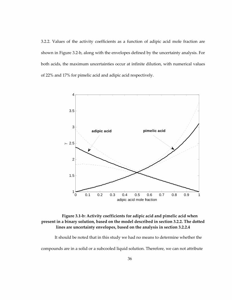
3.2.2. Values of the activity coefficients as a function of adipic acid mole fraction are

shown in Figure 3.2-b, along with the envelopes defined by the uncertainty analysis. For

both acids, the maximum uncertainties occur at infinite dilution, with numerical values

of 22% and 17% for pimelic acid and adipic acid respectively.

Figure 3.1-b: Activity coefficients for adipic acid and pimelic acid when

present in a binary solution, based on the model described in section 3.2.2. The dotted

lines are uncertainty envelopes, based on the analysis in section 3.2.2.4

It should be noted that in this study we had no means to determine whether the

compounds are in a solid or a subcooled liquid solution. Therefore, we can not attribute

0 0.1 0.2 0.3 0.4 0.5 0.6 0.7 0.8 0.9 11

1.5

2

2.5

3

3.5

4


γ

adipic acid pimelic acid

37

the observed values of the activity coefficients to one or the other state. However, the

mixtures were most probably in a solid state, because the melting point depression for

any of the two compounds is expected to be not more than about 10 oC for the range of

molar fractions tested in our experiments. Because the melting points of adipic acid and

pimelic acid are, respectively, 152 oC and 104 oC (Linstrom and Mallard, 2009), the

mixture should remain solid at the temperature of our experiments (35 oC).

The condition of the particles (solid or liquid) can affect the calculation of the

activity coefficients. If the particles are solid, diffusion limitations may cause a radial

gradient of chemical composition within the particles. The solid-state diffusion

coefficients of the acids are of the order of 10-14 m2/s (Lide, 2007). The corresponding

mixing time scale for 100 nm particles, the VMD of our aerosol distribution, can be

estimated using τ ≈ r2/D (in which τ is the characteristic time, r is the particle radius and

D is the diffusion coefficient) to be of the order of 1 s. Therefore, it is reasonable to

assume that the average residence time in our thermodenuder (30 s) is long enough to

have a fairly uniform composition within the particles and, thus, to assume that the

diffusion limitation within particles have a negligible effect on the calculated values of

activity coefficients.

The non-uniform distribution of points along the x-axis in Fig 2-a is explained by

the difficulty of producing aerosol with a high mole fraction of pimelic acid. The reason

38

is that for the temperature change in this experiment (25 oC to 35 oC), pimelic acid

undergoes a larger relative increase of Psat than adipic acid (in terms of aerosol volume

change: ∆v is 90 μm3/cm3 for pure pimelic acid versus 20 μm3/cm3 for pure adipic acid).

Therefore, more pimelic acid is evaporated from the particles relative to the less volatile

adipic acid, decreasing its mole fraction in the particle phase. At high aerosol

concentrations (relative to the change in vapor pressure concentrations) the change in

aerosol composition after the re-equilibration is small. However, to keep the

concentrations such that the CPCs in the SMPS systems are not overloaded, we had to

work at concentration levels which cause an appreciable change in aerosol composition,

especially at the high mixing ratios of the more volatile compound. This makes it

difficult to obtain data points for low adipic acid mole fractions, which is the reason for

the non-uniform distribution of experimental data points. This problem can be alleviated

by installing a dilution system in front of the SMPS to avoid overloading at high

concentration.

We have compared the measured activity coefficients with the UNIFAC group

contribution method (Fredenslund et al., 1975) predictions. The activity coefficients

predicted by the UNIFAC were 1.02 or lower, significantly below the values observed in

this study. Although it would be expected that mixtures of dicarboxylic acids should

exhibit activity coefficients close to unity given the similarity in structure, activity

39

coefficients much different than one were also observed in multi-component

dicarboxylic acid mixtures (Cappa et al., 2008).

3.3.2 Adipic acid – dioctyl sebacate and adipic aci d – ammonium sulfate

Pure dioctyl sebacate did not exhibit measurable volume change when heated

from 25 ⁰C to 35 ⁰C, and it can thus be assumed to be non-volatile in this temperature

range; consequently dioctyl sebacate is not expected to partition to the gas phase. Adipic

acid on the other hand is expected to partition, but, as depicted in Figure 3.2,

partitioning of adipic acid (change in total aerosol volume) is not affected by the

presence of dioctyl sebacate. This leads to the conclusion that the two species do not

form a solution, which is expected since adipic acid is polar while dioctyl sebacate is

non-polar. This was confirmed by attempting to dissolve adipic acid crystals in pure

dioctyl sebacate oil: the crystals did not dissolve even at ratios higher than used in this

study. It should be noted, that the sebacate / adipic acid aerosol was produced by

nebulizing and drying an ethanol solution of these compounds as described in section

3.1. Both compounds formed a uniform mixture with ethanol (i.e. no suspension or

physical separation of phases was observed). Therefore, the aerosol produced by

atomizing this solution is internally mixed, i.e. both compounds are present in each

particle. The fact that no interaction between the compounds was observed means that

the oil and the acid were in separate phases in each particle.

40

Figure 3.2: Change in total aerosol volume for adipic acid – dioctyl sebacate

mixtures between 25 ⁰C and 35 ⁰C.

Ammonium sulfate is also non volatile in the temperature range of our

experiments. Similar to dioctyl sebacate, our data suggest that ammonium sulfate did

not form a solution with adipic acid. As shown in Figure 3.3, there is no suppression or

enhancement of the evaporation of adipic acid. It is interesting to note that Cappa et al.

(2008) observed mutual dissolution of sodium nitrate and several dicarboxylic acids.

One reason for this discrepancy can be that in our binary aerosol ammonium sulfate and

adipic acid were present in the same particles, but, apparently, in separate crystalline

0.1 0.2 0.3 0.4 0.5 0.6 0.7 0.8 0.9 110

12

14

16

18

20

22

24

26


∆V

(µ

m3 /c

m3 )

41

phases, while in the Cappa et al. (2008) study the multi-component mixture was in

subcooled liquid state, which may have promoted dissolution and interaction of sodium

nitrate in the mixture. Another possible reason for discrepancy is that different inorganic

salts behave differently; consequently, interaction between organic and inorganic

fractions in ambient aerosols could be particle size dependent: ammonium sulfate is a

dominant inorganic component in fine aerosol, while sodium nitrate is found mostly in

coarse particles.

Figure 3.3: Change in total aerosol volume for adipic acid – ammonium sulfate

mixtures between 25 ⁰C and 35 ⁰C.

0.2 0.3 0.4 0.5 0.6 0.7 0.8 0.9 112

14

16

18

20

22

24

26

28


∆V

(µm

3 /cm

3 )

42

These experiments indicate that compounds present in ambient or smog chamber

aerosols might not form solution. The implication is that when estimating partitioning of

individual compounds, or classes of compounds, activities need to be calculated with

respect to the solutions they are part of, and not the whole mass of the aerosol.

However, these findings are not conclusive because compounds that do not dissolve

each other in a binary mixture might still form solution in a more complex matrix.

3.3.3 Adipic acid – ambient extracts

Figure 3.4-a shows the total change in aerosol volume of adipic acid – ambient

matrix mixtures versus adipic acid mole fraction. The volume change of the pure

ambient extract (0.7 μm3/cm3) is not shown on the Figure in order to emphasize the

region where most of the measurements were performed (adipic acid mole fractions

higher than 0.7). The reason why there are no data points for adipic acid mole fraction of

less than 0.7 is that the concentration of ambient extract was too low to produce more

points. Our experimental setup requires about 150 ml of solution per experiment. The

solution should be concentrated enough to produce an aerosol concentration that would

be sufficient to saturate the gas stream at the temperature of our experiments. Because

the ambient extract concentration was rather low, we could not dilute the extract to

produce enough aerosol volume for experiments at lower adipic acid fractions. This is a

limitation of the method, which can be solved by collecting a larger ambient aerosol

43

sample (i.e. by sampling higher ambient aerosol concentrations and / or for longer

period of time).

Figure 3.4-a: Change in total aerosol volume for adipic acid – ambient extracts

mixtures between 25 ⁰C and 35 ⁰C. The solid line is the fit based on the model

described in section 3.2.2. The dotted lines are uncertainty envelopes, based on the

analysis in section 3.2.2.4. The volume change of the pure ambient extract (0.7

μm3/cm3) is not shown, but was taken into account when calculating the fit and the

uncertainty envelopes.

Figure 3.4-a also shows the theoretical fit based on the model described in section

3.2.2, and the envelopes defined by the uncertainty analysis as outlined in section 3.2.2.4.

Though the point of pure ambient extract is not included in Figure 3.4-a, it was used in

0.7 0.75 0.8 0.85 0.9 0.95 12

4

6

8

10

12

14

16

18

20


∆V

(µm

3 /cm

3 )

44

calculating the fit and the uncertainty bounds. It is clear that the behavior of adipic acid

in the ambient aerosol matrix is highly non-ideal, with activity coefficients significantly

lower than 1 (Figure 3.4-b).

Figure 3.4-b: Activity coefficients for adipic acid when present in a solution

with ambient extracts, based on the model described in section 3.2.2. The dotted lines

are uncertainty envelopes, based on the analysis in section 3.2.2.4

Using the analysis described in section 3.2.2.3, we obtained an effective ambient

WSOC molar mass of 176 ± 26 g/mol. This value depends on the assumption that the

volume fraction of WSOC in the aerosol is 40%. Assuming WSOC volume fractions of

30% and 50% gives molar masses of 149 ± 10 g/mol and 212 ± 40 g/mol respectively.

0.7 0.75 0.8 0.85 0.9 0.95 1

0.2

0.3

0.4

0.5

0.6

0.7

0.8

0.9

1


γ

45

These values are not meant to be quantitative estimates; however, they might suggest

that the compounds constituting WSOC in our samples are mostly high molar mass

multifunctional compounds. The estimated molecular weight is within the range

reported for water soluble organic aerosol. Ambient samples from K-pustza and

Jungfraujoch were reported to have average molecular weights in the range 200-300

g/mol (Kiss et al., 2003, Krivácsy et al., 2001).

Saxena and Hildemann (1996) reported that the major constituents of WSOC in

atmospheric aerosols are C2 to C7 multifunctional compounds. The compounds

suggested by Saxena and Hildemann have saturation pressures at 25 ⁰C comparable to

those of adipic and pimelic acid or (up to several orders of magnitude) higher. Their

selection of compounds seems to contradict our observations: the aerosol generated

from the ambient aqueous extract has very low volatility compared to pure adipic acid

and pimelic acid. The total volume change of the ambient matrix at thermodenuder set-

temperature of 35 ⁰C is 0.7 μm3/cm3 versus 18 μm3/cm3 for adipic acid and 90 μm3/cm3 for

pimelic acid. Since the change in volume observed in our experiments is the average

volatility of all the components in the mixture, the measurements show that the WSOC

portion of the ambient aerosol is less volatile than the components proposed by Saxena

and Hildemann. Our results (both the volatility and molecular weight) are more

consistent with longer chain dicarboxilic acids (such as azelaic acid) or C8-C10 polyols.

46

On the other hand, the compounds selected by Saxena and Hildemann have been

observed in ambient aerosols (Grosjean et al., 1978; Kawamura and Kaplan, 1987;

Sempere and Kawamura, 1994; Rogge et al, 1993). The behavior of adipic acid when in

mixture with the WSOC ambient matrix observed in this study shows activity

coefficients significantly lower than one (Figure 6), which agrees with the findings of

Cappa et al. (2008) for lab generated multicomponent dicarboxylic acid mixtures. This

suggests that evaporation of adipic acid is strongly reduced in the ambient matrix,

which would shift its partitioning to the aerosol phase. Whether such behavior is

observed for other dicraboxylic acids and other ambient aerosol matrices was beyond

the scope of this study and needs to be investigated.

3.4 Conclusions

This chapter demonstrates the application of the integrated volume method to

estimate activity coefficients of binary organic mixtures pertinent to

ambient/atmospheric aerosols. The method is applied to adipic acid – pimelic acid as an

example for polar – polar organic mixtures, adipic acid – dioctyl-sebacate as an example

for polar – non-polar mixtures, adpic acid – ammonium sulfate as an example of polar

organic – inorganic mixtures, and adipic acid – ambient extracts to illustrate application

to realistic ambient systems. Adipic acid – pimelic acid mixture exhibited highly non-

ideal behavior with activity coefficients of about 3 at infinite dilution, which stresses the

47

importance of activity coefficients in portioning of semi-volatile organics in ambient

aerosols. On the other hand, adipic acid – dioctyl-sebacate and adipic acid – ammonium

sulfate mixtures did not form a solution; adipic acid partitioned to the gas phase in the

same manner as in the pure case. Care needs to be taken when calculating mole fractions

of compounds in ambient or smog chamber aerosols to estimate their activities, since an

aerosol particle might be comprised of multiple phases/solutions depending on the

affinities of the species. When mixed with ambient extracts, adipic acid exhibited activity

coefficients significantly less than unity, which suggests that the volatility of this

compound could be strongly suppressed in ambient aerosol, favoring its partitioning to

the aerosol phase. The tested water extract of ambient aerosol exhibited behavior

consistent with average molecular weight of about 180 g/mol and average volatility of

C8 – C10 dicarboxylic acids.

48

4. Effect of aerosol generation method on measured thermodynamic properties

In this chapter, we investigate the effect of residual solvent on saturation

pressure and enthalpy of vaporization obtained for C-6 (adipic) and C-9 (azelaic)

dicarboxylic acid aerosols generated by two methods: 1) atomization and drying of

aqueous solutions, and 2) homogenous condensation of organic vapor. Because the

second method involves no solvent, it provides a control condition in which any

potential solvent effect has been eliminated. A comparison of the thermodynamic

properties measured with the two generation methods provides a measure of the effect

of retained water, if any is present in the particles. The Psat and ∆H were determined

using the Integrated Volume Method (IVM) (Saleh et al., 2008). We also obtained SEM

images of the aerosol particles produced by the two methods to compare their

morphology.

4.1 Methods

The experimental setup is shown in Figure 4.1. It consists of an aerosol

generation system, two Scanning Mobility Particle Sizer (SMPS) systems, and a

thermodenuder. The individual parts of the set-up are described in separate sections

below.

49

4.1.1 Aerosol generation

The aerosol was generated by two different techniques: 1) the conventional

aqueous solution atomization and 2) homogeneous condensation. For the former, 0.1

wt % aqueous (in de-ionized 18 MΩ water) solutions of the dicarboxylic acids were

atomized using a 6-jet atomizer (TSI, model 9306). Two out of the 6 jets were operated

and the aerosol flowrate was 3 SLPM, while the dilution flowrate was set to 15 SLPM

(the dilution system is integral to the atomizer). The purpose of dilution flow (particle-

free and < 10% RH) was to decrease the particle number concentration to within the

detection limit of our SMPS systems, as well as to dry the aerosol. A flow of 2 SLPM

was drawn from the diluted stream through a diffusion-dryer for additional drying,

while the excess was sent to exhaust. Typically, the Volume Median Diameter (VMD) of

the aerosol particles was approximately 180 nm, the total volume concentration was

approximately 200 μm3/cm3, and the geometric standard deviation (σg) was

approximately 1.8.

For the homogeneous condensation generation method, a Condensation

Monodisperse Aerosol Generator (CMAG, TSI, model 3475) was utilized. Although the

conventional use of the CMAG is to generate monodisperse aerosols by condensation on

seed particles, it can also be operated without seed particles to produce a polydisperse

aerosol by homogeneous nucleation. For a material that is solid at room temperature, the

50

CMAG operating procedure normally entails heating the material to above its melting

point and bubbling a controlled flow of nitrogen through the liquid in a saturator. The

vapor-laden nitrogen then passes through a condenser where it cools to room

temperature, causing super-saturation and subsequent nucleation of aerosol particles.

For the purposes of this study, we used a sublimation technique in which the nitrogen

flowed over a bed of solid acid crystals instead of bubbling through melted acids. This

modification had two benefits. First, it allowed acid vapor generation at relatively low

temperatures, thus avoiding thermal degradation (preliminary experiments at

temperatures slightly above melting point with adipic acid caused discoloration of the

acid upon re-solidification). Second, with sublimation we were able to obtain aerosol

concentrations within the detection limit of our sizing system without the need for

dilution.

51

Figure 4.1: Schematic of IVM experimental setup. For homogeneous

condensation, the 6-jet atomizer is replaced with a CMAG, and the diffusion dryer is

removed

The CMAG was operated with total and bypass nitrogen flows of 3.6 SLPM and

0.25 SLPM respectively. The optimum saturator temperature that produced a large

enough aerosol concentration with a size distribution within the detection limit of our

sizing system was found by trial and error to be approximately 140 ⁰C for adipic acid

and 100 ⁰C for azelaic acid. A flow of 2 SLPM was drawn for sampling, while the excess

was sent to exhaust. VMD of the aerosol ranged between 150 nm and 200 nm, the total

volume concentration between 150 μm3/cm3 and 250 μm3/cm3, and σg between 1.7 and

1.8.

52

4.1.2 Aerosol sizing and conditioning

The 2 SLPM aerosol flow was split into two 1 SLPM lines. One was sampled for

reference measurements by the upstream SMPS, and the other was sent through a

thermodenuder of 1 m length and 3.5 cm inner diameter. The final size distribution was

measured by the downstream SMPS. The thermodenuder was heated to a desired

maximum temperature and then allowed to cool down gradually to room temperature;

the upstream and the downstream aerosol size distributions as well as the

thermodenuder temperature were continuously measured and recorded from the onset

of cooling. The average residence time in the thermodenuder was 58 s. As described in

Saleh et al. (2008), IVM requires that the time required for the aerosol to reach

equilibrium should be less than the residence time in the thermodenuder. To confirm

that equilibrium was achieved at the reference state, the total particle volume was

measured at reference temperature by the upstream SMPS and the downstream SMPS

(after the aerosol has spent an extra 58 s in the thermodenuder) and found to be equal to

within instrument uncertainty (~20%). To verify the equilibration assumption in the

thermodenuder we used the evaporation kinetics model described in Saleh et al. (2008)

to estimate equilibration times of our test aerosols over the range of experimental

temperatures. The particle size distributions used in the simulations are given in section

4.1.1 for both atomization and homogeneous nucleation techniques. The value of

53

evaporation coefficient used for adipic acid was 0.08 (Saleh et al., 2009). While the

evaporation coefficient of azelaic acid has not been previously reported, our recent

measurements of evaporation coefficient for adipic, pimelic, and succinic acids, suggest

that the evaporation coefficients of dicarboxylic acids in air are of the order 10-1. For the

purpose of the simulations, we assumed a value for the evaporation coefficient of azelaic

acid to be equal to that of adipic acid. The simulations predicted equilibration times of

less than 30 s for all cases, which is considerably less than the 58 s residence time of the

thermodenuder. Detailed analysis on equilibration in thermodenuders is presented in

the next chapter.

4.1.3 The integrated volume method

The thermodynamic properties of the test compounds were determined using the

Integrated Volume Method (IVM), which is described in detail in Chapter 2. Briefly, the

IVM uses temperature dependent aerosol volume changes to derive the saturation vapor

pressure, Psat, and enthalpy of vaporization, ∆H, of the test compound. The integrated

aerosol volume changes, pv∆ , are measured at several temperatures and the results are

fit into the following equation to obtain Psat, and ∆H:

0 0

1 1( ) exp 1sat

p

p

P M Hv T

RT R T Tρ

∆∆ = − − −

(4.1)

54

in which T is the thermodenuder temperature, and 0T is the reference temperature, M

is the molecular weight of the compound, ρp is the particle density (1360 kg/m3 and 1225

kg/m3 for adipic and azelaic acid respectively) , R is the universal gas constant.

The IVM is advantageous in that the aerosol is investigated at equilibrium.

Therefore, knowledge of other properties associated with the evaporation kinetics,

namely the diffusion coefficient, surface free energy, and evaporation coefficient, is not

required to estimate Psat and ∆H. In contrast, methods that employ evaporation kinetics

such as the Tandem Differential Mobility Analyzer (TDMA) method (Tao and McMurry,

1989; Bilde et al., 2003) and Temperature Programmed Desorption (TPD) method

(Cappa et al., 2007 & 2008), normally require the assumption that the evaporation

coefficient is unity when estimating Psat.

4.1.4 SEM imaging

Samples for SEM imaging were collected on 47 mm Nuclepore Polycarbonate

filters which were inserted downstream of the aerosol generators (downstream of the

diffusion dryer in the case of aqueous solution atomization). Sampling times were 1 - 3

hours at 1 SLPM.

Square 1 cm × 1 cm sections were cut out of the filters and mounted on the SEM

stubs. Prior to imaging, the samples were coated with gold to enhance conductivity and

suppress potential volatilization at the low operating pressure of the SEM.

55


4.2.1 Saturation pressures and enthalpies of vapori zation

Plots of the integrated aerosol volume change versus the inverse of

thermodenuder temperature obtained from the IVM experiments are depicted in Figure

4.2 for aerosol generated by aqueous solution atomization and by homogeneous

condensation. Also shown are the theoretical fits based on equation (4.1), where Psat,0 and

∆H are fitting parameters. For adipic acid, we obtained Psat,0 of 3.3×10-5 (±0.9×10-5) Pa and

∆H of 132 (±8) kJ/mol with atomization, and Psat,0 of 4.2×10-5 (±2.2×10-5) Pa and ∆H of 126

(±21) kJ/mol with homogeneous condensation. For azelaic acid, we obtained Psat,0 of

1.4×10-5 (±0.5×10-5) Pa and ∆H of 145 (±15) kJ/mol with atomization, and Psat,0 of 0.9×10-5

(±0.3×10-5) Pa and ∆H of 158 (±17) kJ/mol with homogeneous condensation.

It should be noted that the IVM experiments in this study were performed with a

different SMPS / thermodenuder system than in Saleh et al. (2008) (Chapter 2). The

excellent agreement in Psat,0 and ∆H (Table 4.1) obtained with the 2 different

experimental setups is thus assuring.

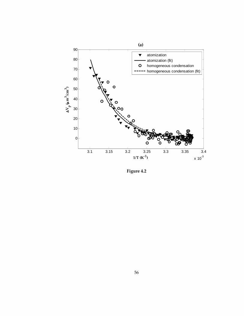
56

Figure 4.2

3.1 3.15 3.2 3.25 3.3 3.35 3.4

x 10-3

0

10

20

30

40

50

60

70

80

90

1/T (K-1)

∆∆ ∆∆V

p (µµ µµ

m3/c

m3)

(a)

atomization

atomization (fit)homogeneous condensation

homogeneous condensation (fit)

57

Figure 4.2 (continued): Measured change in total volume concentration of adipic

acid (a) and azelaic acid (b) aerosol particles versus inverse of set-temperature

As shown in Figure 4.2-a and Figure 4.2-b, both adipic acid and azelaic acid

exhibit similar total particle volume change as a function of temperature when using

either of the two aerosol generation methods. Consequently, the values obtained for Psat,0

and ∆H (Table 4.1) are within the experimental uncertainty. This indicates that the

quantity of residual water in the aerosol when generated by conventional atomization

and drying, if any, is insufficient to significantly impact the thermodynamic properties

of the investigated dicarboxylic acids. This seems to contradict the observation of Cappa

3.1 3.15 3.2 3.25 3.3 3.35 3.4

x 10-3

0

10

20

30

40

50

1/T (K-1)

∆∆ ∆∆V

p( µµ µµ

m3/c

m3)

(b)

atomization

atomization (fit)homogeneous condensation

homogeneous condensation (fit)

58

et al. (2007) that when they pre-heated the atomized aerosol, the measured Psat,0

decreased by an order of magnitude, which was attributed to retained solvent. At the

simplest level, this contradiction can be due to inadequate drying in the aerosol

generation setup employed in Cappa et al. (2007), leaving the particles with an amount

of residual solvent substantial enough to cause bias in measured Psat,0. Another potential

reason for this discrepancy is that the observed pre-heating effect in Cappa et al. (2007)

was not due to the presence of solvent, but that pre-heating-induced evaporation

changed the size, and possibly the shape, of the particles, which were deposited to form

a cone-shaped mound from which evaporation rate was measured. The surface area of

the mound was estimated based on a smooth cone assumption; the results are thus

sensitive to the actual packing of the particles. The small pre-heated particles could be

more densely packed than larger particles, decreasing the total surface area of the

mound, thus decreasing the evaporation rate, which would result in a lower measured

Psat,0.:


dicarboxylic acids.

Acid Study Psat,0 (10-5 Pa) ∆H (kJ/mol)

Adipic Saleh et al. (2008)

This study (atomization)

This study (homogeneous

condensation)

3.4 (± 1.2)

3.3 (± 0.9)

4.2 (± 2.2)

135 (± 13)

132 (± 8)

126 (± 21)

Azelaic This study (atomization)

This study (homogeneous

condensation)

1.4 (± 0.5)

0.9 (± 0.3)

145 (± 15)

158 (± 17)

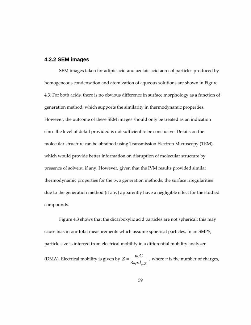
59

4.2.2 SEM images

SEM images taken for adipic acid and azelaic acid aerosol particles produced by

homogeneous condensation and atomization of aqueous solutions are shown in Figure

4.3. For both acids, there is no obvious difference in surface morphology as a function of

generation method, which supports the similarity in thermodynamic properties.

However, the outcome of these SEM images should only be treated as an indication

since the level of detail provided is not sufficient to be conclusive. Details on the

molecular structure can be obtained using Transmission Electron Microscopy (TEM),

which would provide better information on disruption of molecular structure by

presence of solvent, if any. However, given that the IVM results provided similar

thermodynamic properties for the two generation methods, the surface irregularities

due to the generation method (if any) apparently have a negligible effect for the studied

compounds.

Figure 4.3 shows that the dicarboxylic acid particles are not spherical; this may

cause bias in our total measurements which assume spherical particles. In an SMPS,

particle size is inferred from electrical mobility in a differential mobility analyzer

(DMA). Electrical mobility is given by 3 ev

neCZ

dπµ χ= , where n is the number of charges,

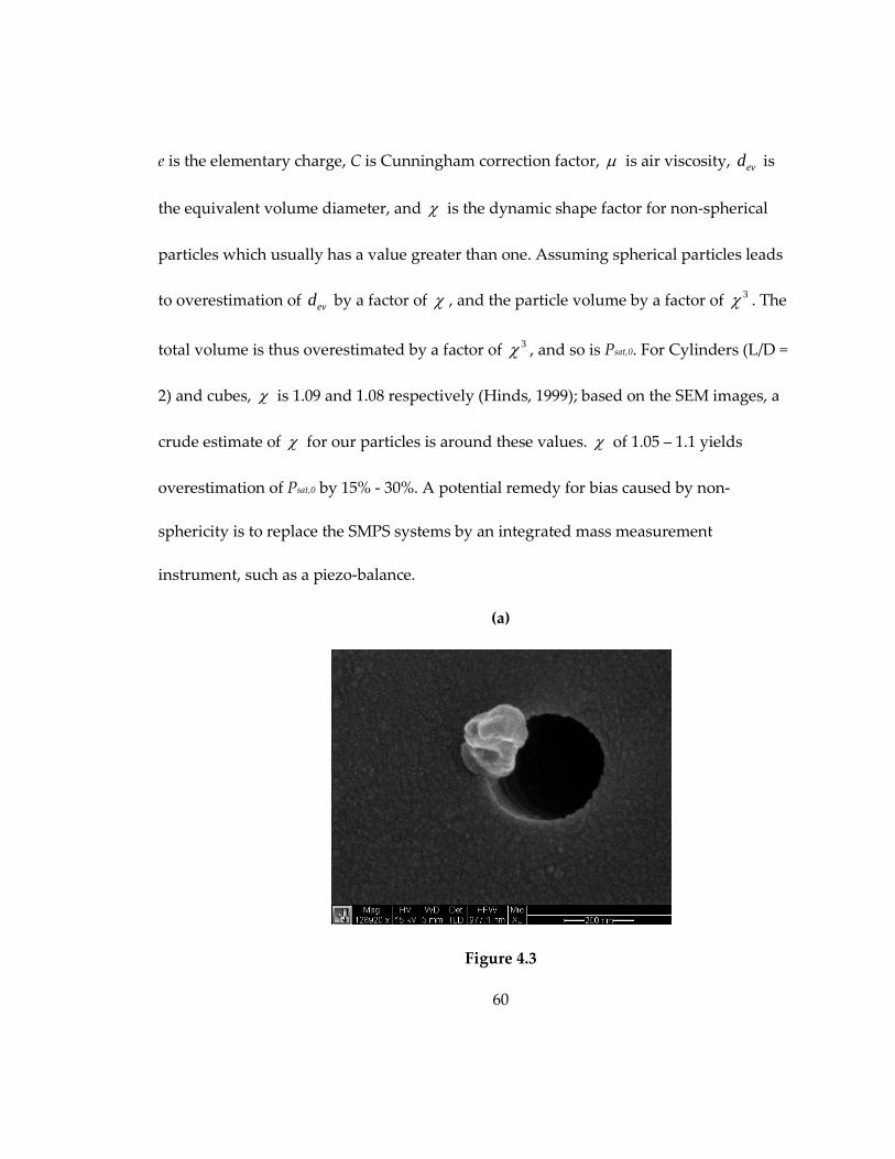
60

e is the elementary charge, C is Cunningham correction factor, µ is air viscosity, evd is

the equivalent volume diameter, and χ is the dynamic shape factor for non-spherical

particles which usually has a value greater than one. Assuming spherical particles leads

to overestimation of evd by a factor of χ , and the particle volume by a factor of 3χ . The

total volume is thus overestimated by a factor of 3χ , and so is Psat,0. For Cylinders (L/D =

2) and cubes, χ is 1.09 and 1.08 respectively (Hinds, 1999); based on the SEM images, a

crude estimate of χ for our particles is around these values. χ of 1.05 – 1.1 yields

overestimation of Psat,0 by 15% - 30%. A potential remedy for bias caused by non-

sphericity is to replace the SMPS systems by an integrated mass measurement

instrument, such as a piezo-balance.

(a)

Figure 4.3

61

(b)

Figure 4.3 (continued)

(c)


(d)

62

Figure 4.3 (continued): SEM images for (a) adipic acid generated by

homogeneous condensation, (b) adipic acid generated by atomization, (c) azelaic acid

generated by homogeneous condensation, and (d) azelaic acid generated by

atomization

4.3 Conclusions

We have investigated the effect of aerosol generation method on thermodynamic

properties of adipic acid and azelaic acid aerosols. Saturation pressures at 298 K and

enthalpies of vaporization were determined for the dicarboxylic acids generated by 1)

atomization of aqueous solutions and 2) homogeneous condensation of organic vapor.

We found no significant difference between the thermodynamic properties as a function

of generation method. This implies that retained water in the test aerosol generated

using conventional atomization/drying techniques, if any, does not affect the measured

thermodynamic properties. Also, SEM images showed no apparent difference in surface

morphology between aerosol particles generated by the two methods.

63

5. On transport phenomena and equilibration time scales in thermodenuders

5.1 Introduction

Thermodenuders have been widely used in aerosol volatility studies, both in the

lab (e.g. An et al., 2007; Saleh et al., 2008; Fuallhaber et al., 2009) and in the field (e.g.

Wehner et al., 2004; Huffman et al., 2008; Dzepina et al., 2009). A thermodenuder (TD) is

simply a temperature controlled flow tube. When a volatile/semi-volatile aerosol is

introduced into a heated TD, the particles respond by evaporating. The extent to which

the particles evaporate – the difference between initial and final size distributions –

provides information about their volatility. Although the operation of the TD is

relatively simple, it has been the subject of some confusion. There are two main,

sometimes controversial, issues associated with TDs: 1) equilibration and 2) the need for

an activated carbon denuder in the cooling section connecting the TD to the sizing

instrument. The intent of including a denuder is to minimize re-condensation of the

evaporated vapor back to the particles from which it originated, and thereby avoid

particle size changes from the outlet of the TD to the sizing instrument.

Researchers have recently recognized the importance of kinetic limitations to

volatility studies in TDs. For reliable volatility measurements, the aerosol should

approach equilibrium within the residence time available in the TD, otherwise volatility

would be underestimated (An et al., 2007; Saleh et al., 2008; Riipinen et al., 2010). Saleh

64

et al. (2008, 2009, 2010) and Saleh and Khlystov (2009) found by numerical simulation

and empirical measurements that the residence time in a typical TD is sufficient for

equilibration at the experimental conditions of their study (aerosol concentrations higher

than 200 µg/m3 and a residence time of 30 s). On the other hand, Riipinen et al. (2010)

and Cappa (2010) argued, based on their evaporation kinetics models, that equilibration

is not likely to be achieved for most ambient/laboratory aerosol systems within

reasonable residence times. They concluded that kinetic models are necessary to

interpret TD volatility measurements. It should be noted that these two studies arrived

at opposite conclusions with regard to the effect of the aerosol volatility on the

equilibration time scales: Riiponen et al. (2010) found that the lower volatility

compounds could be equilibrated on time scales of milliseconds, if the aerosol

concentration is sufficiently high, while Cappa (2010) argued that low volatility

compounds cannot be equilibrated at any reasonable time scales. However, as will be

shown in this chapter, equilibration time is not affected by volatility.

The second controversy relates to the cooling section of thermodenuders, where

the aerosol is returned to room temperature. In the cooling section, the concentration

gradient is reversed, causing condensation on the aerosol particles and the walls of the

cooling section. It has been feared that this re-condensation will lead to bias in the

measurements, and therefore most researchers have used activated carbon (AC)

65

denuders for cooling sections to strip the organic vapor and minimize re-condensation

on the particles (e.g. An et al., 2007; Faullhaber et al., 2009; Huffman et al., 2009). It

should be noted that the inclusion of an AC denuder in these studies was not justified

theoretically or experimentally. Some studies, (e.g. Sakurai et al., 2003 and Saleh et al.,

2008, 2009, 2010) found that the effect of re-condensation is negligible in their systems,

and thus operated without an AC denuder. Using an aerosol evaporation kinetics

model, Cappa (2010) found that bias due to re-condensation is small at low aerosol

loadings, but might become substantial at high loadings.

Most of the TD studies have used aerosol particles mass fraction remaining

(MFR) as an indication of aerosol volatility. MFR is defined as the ratio of aerosol

particle mass concentration exiting the TD to the initial (reference) mass concentration.

MFR has been used in 2 ways to infer aerosol volatility: 1) at a constant TD temperature,

volatilities of different aerosol species are compared based on their MFR – the lower the

MFR, the more volatile is the aerosol (e.g. An et al., 2007); 2) the TD temperature is

varied until a certain MFR is reached (say 50%), and the required TD temperatures are

compared – the lower the temperature the more volatile is the aerosol (Faullhaber et al.,

2009). The use of MFR to estimate volatility is theoretically unjustifiable however and

leads to spurious results. The reason is that volatility (Csat) does not depend on particle

mass concentration, but on equilibrium between the particle phase and the gas phase. To

66

illustrate, consider an aerosol with Csat(T) of 50 μg/m3, and 2 initial particle

concentrations 100 μg/m3 and 500 μg/m3. If both achieve equilibrium in a TD, ∆C will be

50 μg/m3 in both cases (assuming that initial Csat is much smaller than Csat(T)), while MFR

will be 0.5 and 0.9 respectively. Using MFR, the same aerosol would be mistakenly

thought to have different volatility. The change in aerosol concentration, ∆C, on the

other hand is an appropriate metric for volatility studies (Saleh et. al 2008; Saleh and

Khlystov, 2009).

In this chapter, we present a theoretical and experimental exploration of heat and

mass transport, and evaporation kinetics in thermodenuders. A plug flow

computational model (Saleh and Shihadeh, 2007) is used to investigate equilibration

time scales in TDs as well as potential re-condensation in the cooling section.

Dimensional analysis is performed to identify the governing parameters in the

equilibration problem. Theoretical findings are compared to experiments performed

with pure and mixed semi-volatile dicarboxylic acid aerosols.

5.2 Theory

Consider a volatile or semi-volatile aerosol initially at equilibrium with its

surrounding gas phase. The total particle mass concentration is C0 and the vapor

concentration in the gas phase is Csat,0, the saturation concentration at the equilibrium

temperature T0. When the aerosol flows through the heating section of a TD maintained

67

at T1 > T0, a concentration gradient is created between the surface of the particles and the

gas phase, and the particles respond by evaporating to bring the system to equilibrium

at T1, which corresponds to vapor concentration of Csat,1 in the gas phase. If the residence

time in the TD is longer than equilibration time, and provided that C0 > Csat,1, the aerosol

approaches equilibrium; in other words, the gas phase approaches a saturation ratio SR

= Cg / Csat,1 = 1, where Cg is the vapor concentration in the gas phase. If the residence time

in the TD is shorter than the equilibration time, the aerosol exits the TD with SR < 1. In

the cooling section, the aerosol temperature is brought back to T0, causing the gas phase

to supersaturate with the vapor, and thereby reversing the concentration gradient.

Vapor starts to condense on the particles as well as the walls of the cooling section.

The heat and mass transport phenomena in the heating and cooling sections of

the TD are similar, and can be modeled using the same set of equations but with

different boundary conditions. In section 5.2.1, we describe a plug flow model where the

fluid dynamics is simplified by assuming a well-mixed flow. Dimensional analysis on

the plug flow model is presented in section 5.2.2 and is utilized to identify key

parameters that govern equilibration in TDs. In section 5.2.3, the relative importance of

condensation on aerosol particles and the walls in the cooling section is investigated in

terms of the coupling number previously derived by Saleh and Shihadeh (2007).

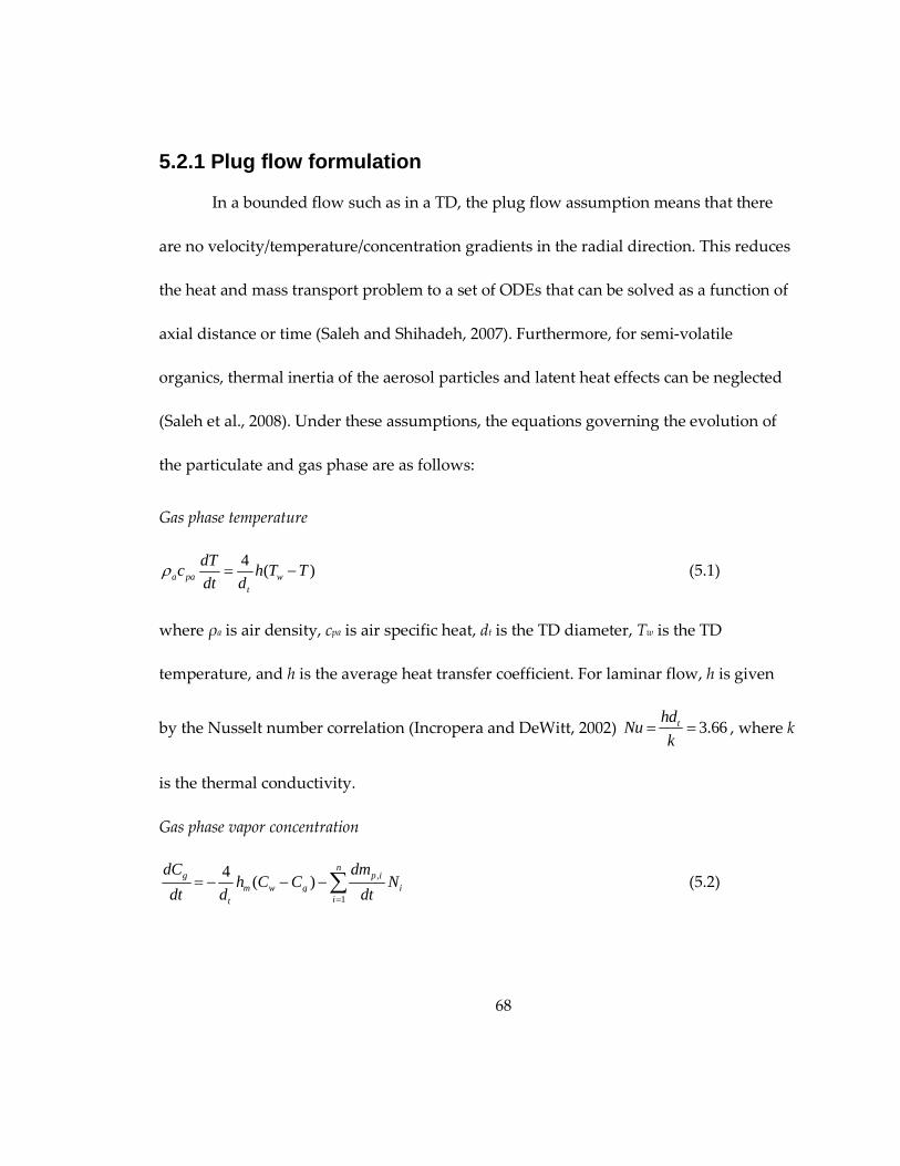
68

5.2.1 Plug flow formulation

In a bounded flow such as in a TD, the plug flow assumption means that there

are no velocity/temperature/concentration gradients in the radial direction. This reduces

the heat and mass transport problem to a set of ODEs that can be solved as a function of

axial distance or time (Saleh and Shihadeh, 2007). Furthermore, for semi-volatile

organics, thermal inertia of the aerosol particles and latent heat effects can be neglected

(Saleh et al., 2008). Under these assumptions, the equations governing the evolution of

the particulate and gas phase are as follows:

Gas phase temperature

4( )ρ = −a pa w

t

dTc h T T

dt d (5.1)

where ρa is air density, cpa is air specific heat, dt is the TD diameter, Tw is the TD

temperature, and h is the average heat transfer coefficient. For laminar flow, h is given

by the Nusselt number correlation (Incropera and DeWitt, 2002) 3.66thdNu

k= = , where k

is the thermal conductivity.

Gas phase vapor concentration

,

1

4( )

=

= − − −∑n

g p im w g i

it

dC dmh C C N

dt d dt (5.2)

69

The first term on the right hand side is the mass transfer rate to the wall of the

TD. Cw is the vapor concentration at the TD wall and hm is the average mass transfer

coefficient. By analogy to heat transfer, hm can be calculated as 2/ 3ma pa

hh

c Leρ=

(Incropera

and DeWitt, 2002), where thDLe

D= is Lewis number, the ratio of thermal diffusivity to

mass diffusivity. The second term on the right hand side is the net mass transfer rate

to/from the ensemble of aerosol particles, which are distributed into n discrete size bins,

each characterized by a single diameter dpi and number concentration Ni. While the

number concentration is held constant (i.e. no coagulation or deposition), the diameter is

allowed to vary in accordance with mass transfer. The mass transfer from a single

particle is given by the Maxwell equation corrected for non-continuum effects (see

below).

Particle mass

( ),,2π= − −p i

p i sat g

dmd DF KC C

dt (5.3)

where D is the diffusion coefficient; Csat is the saturation concentration;

4exp

p p

MK

Td

σρ

=

is Kelvin correction where ρp is the particle density, M is the molar

mass, and σ is the surface free energy; 1

1 0.3773 1.33 (1 ) /

KnF

Kn Kn Kn α+

=+ + +

is the

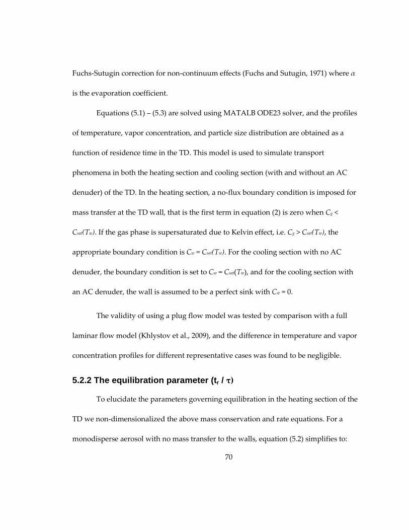
70

Fuchs-Sutugin correction for non-continuum effects (Fuchs and Sutugin, 1971) where α

is the evaporation coefficient.

Equations (5.1) – (5.3) are solved using MATALB ODE23 solver, and the profiles

of temperature, vapor concentration, and particle size distribution are obtained as a

function of residence time in the TD. This model is used to simulate transport

phenomena in both the heating section and cooling section (with and without an AC

denuder) of the TD. In the heating section, a no-flux boundary condition is imposed for

mass transfer at the TD wall, that is the first term in equation (2) is zero when Cg <

Csat(Tw). If the gas phase is supersaturated due to Kelvin effect, i.e. Cg > Csat(Tw), the

appropriate boundary condition is Cw = Csat(Tw). For the cooling section with no AC

denuder, the boundary condition is set to Cw = Csat(Tw), and for the cooling section with

an AC denuder, the wall is assumed to be a perfect sink with Cw = 0.

The validity of using a plug flow model was tested by comparison with a full

laminar flow model (Khlystov et al., 2009), and the difference in temperature and vapor

concentration profiles for different representative cases was found to be negligible.

5.2.2 The equilibration parameter ( tr / τ)

To elucidate the parameters governing equilibration in the heating section of the

TD we non-dimensionalized the above mass conservation and rate equations. For a

monodisperse aerosol with no mass transfer to the walls, equation (5.2) simplifies to:

71

= −g ptot

dC dmN

dt dt (5.4)

Equations (5.3) and (5.4) can be non-dimensionalized using t* = t/tr where tr is the

residence time in the TD, dp* = dp/dp,in where dp,in is the initial particle diameter, and C*g =

Cg/Csat, where Csat is the saturation concentration at the TD temperature. In this analysis,

the time required for the thermal boundary layer to grow to fully developed conditions

is assumed to be much shorter than the total residence time in the TD. This assumption

is reasonable for conventional TD designs. Substituting equation (5.3) in equation (5.4)

and inserting the dimensionless parameters yields:

** * * *

,*2 ( ) ( )π

τ= − = −g r

tot p in r g p g p

dC tN d DFt K C d K C d

dt (5.5)

where ,

1

2 tot p inN d DFτ

π= . It can be readily shown that τ physically represents the

characteristic evaporation time required for an aerosol of fixed diameter and kinetic

properties to produce a change in concentration in the gas phase equal to 1/e of the

initial difference in vapor concentration between the layer immediately surrounding the

droplet phase and the gas phase, (KCsat – Cg). We should note that the expression of τ is

similar to the equilibration time scale previously derived by Wexler and Seinfeld (1990).

tr/τ thus represents the ratio of time available in the TD to the characteristic time of

evaporation in a bounded aerosol.

72

Equation (5.5) shows that the evolution of the dimensionless gas concentration

(C*g) in a heated TD is characterized by a single dimensionless parameter, tr/τ, which has

no dependence on the thermodynamic properties of the aerosol, contrary to the

conclusions of Riipinnen et al. (2010) and Cappa (2010). It only depends on the aerosol

size distribution (the total aerosol length Ntot.dp,in) and kinetic properties of the aerosol, D

and α (through F; see equation (3)). When coupled with experimental data, τ can be used

as a semi-empirical tool to predict the required residence time required for a certain

aerosol to achieve equilibrium, as described in section 5.4.4.

This analysis can be readily extended to polydisperse aerosol, where the effect of

the size distribution is accounted for by using the condensation sink diameter (Lehtinen

et al., 2003)., The condensation sink diameter is the particle diameter of a monodisperse

aerosol that exhibits the same net evaporation or condensation rate as a polydisperse

aerosol, both with a given number concentration. The condensation sink diameter can

be calculated for a certain particle size distribution from the moment average

1/

,1

,

1

ana

i p ii

p cs n

ii

N dd

N

=

=

=

∑

∑, where the exponent a varies between unity for the continuum

regime and 2 for the free molecular regime. For the transition regime, it is obtained by

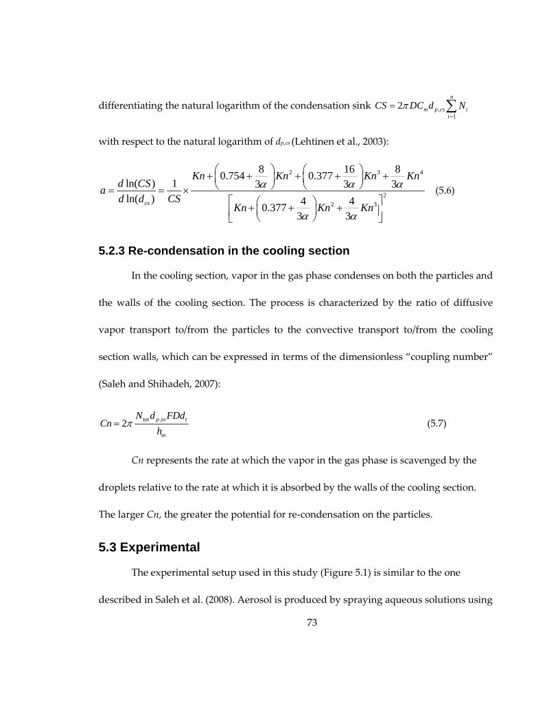
73

differentiating the natural logarithm of the condensation sink ,1

2n

m p cs ii

CS DC d Nπ=

= ∑

with respect to the natural logarithm of dp,cs (Lehtinen et al., 2003):

2 3 4

2

2 3

8 16 80.754 0.377

ln( ) 1 3 3 3ln( ) 4 4

0.3773 3

cs

Kn Kn Kn Knd CS

ad d CS

Kn Kn Kn

α α α

α α

+ + + + + = = ×

+ + +

(5.6)

5.2.3 Re-condensation in the cooling section

In the cooling section, vapor in the gas phase condenses on both the particles and

the walls of the cooling section. The process is characterized by the ratio of diffusive

vapor transport to/from the particles to the convective transport to/from the cooling

section walls, which can be expressed in terms of the dimensionless “coupling number”

(Saleh and Shihadeh, 2007):

,2π= tot p in t

m

N d FDdCn

h (5.7)

Cn represents the rate at which the vapor in the gas phase is scavenged by the

droplets relative to the rate at which it is absorbed by the walls of the cooling section.

The larger Cn, the greater the potential for re-condensation on the particles.

5.3 Experimental

The experimental setup used in this study (Figure 5.1) is similar to the one

described in Saleh et al. (2008). Aerosol is produced by spraying aqueous solutions using

74

a constant output atomizer, and is sent to a 20 liter chamber to mix with dry, particle-

free air at 40 SLPM for dilution and drying. A flow of 1 SLPM is drawn through a

diffusion-dryer to remove any remaining water, while the excess is sent to exhaust. The

1 SLPM aerosol flow is then sent through a TD with a heating section of 1 m length and

2.5 cm inner diameter. The residence time in the heating section of the TD is controlled

by varying the extraction flowrate using a mass flow controller. The maximum average

residence time, which corresponds to a zero bypass flowrate, is around 30 s. The default

cooling section is a copper tube of 1 m length and 0.63 cm inner diameter. We have used

other configurations for the cooling section, as described below. Reference and heated

aerosol size distributions are measured using a Scanning Mobility Particle Sizer (SMPS).

To investigate equilibration time scales, we measured the change in aerosol

particle concentration (∆C) at different residence times in the TD. Equilibration was

considered achieved at a certain residence time if ∆C did not increase with further

increase in residence time. For each tested aerosol, ∆C values were measured at average

residence times of 9, 12, 15, 20, and 30 s. The experimental matrix used to investigate

equilibration in TDs is shown in Table 1. All experiments were performed at reference

temperature of 25 ⁰C and TD set temperature of 40 ⁰C. We chose adipic acid aerosol (C0 =

390 μg/m3, Ntot = 1012 particles/m3, dp,cs = 65 nm) as the base case. To illustrate the

dependence of equilibration time scales on aerosol loading, we varied the initial particle

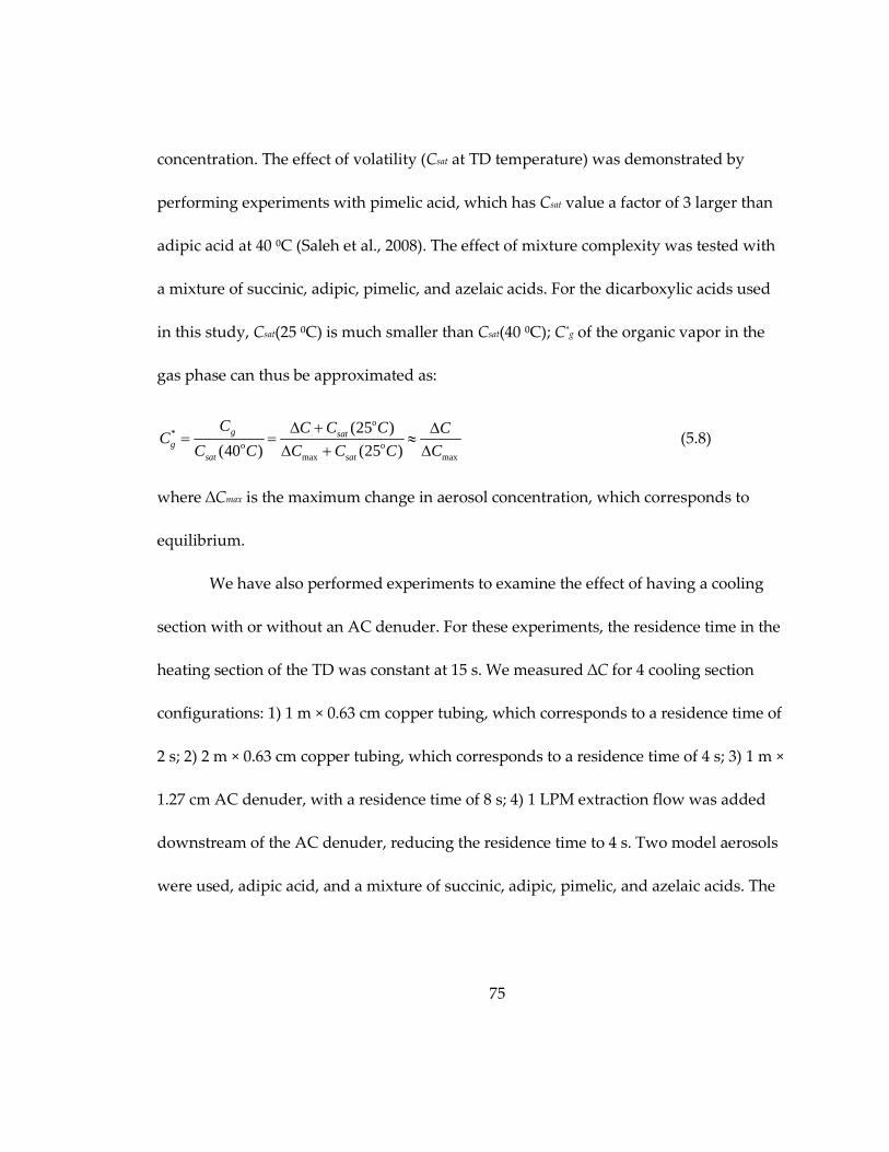
75

concentration. The effect of volatility (Csat at TD temperature) was demonstrated by

performing experiments with pimelic acid, which has Csat value a factor of 3 larger than

adipic acid at 40 ⁰C (Saleh et al., 2008). The effect of mixture complexity was tested with

a mixture of succinic, adipic, pimelic, and azelaic acids. For the dicarboxylic acids used

in this study, Csat(25 ⁰C) is much smaller than Csat(40 ⁰C); C*g of the organic vapor in the

gas phase can thus be approximated as:

*

max max

(25 )

(40 ) (25 )

∆ + ∆= = ≈

∆ + ∆

o

o o

g satg

sat sat

C C C C CC

C C C C C C (5.8)

where ∆Cmax is the maximum change in aerosol concentration, which corresponds to

equilibrium.

We have also performed experiments to examine the effect of having a cooling

section with or without an AC denuder. For these experiments, the residence time in the

heating section of the TD was constant at 15 s. We measured ∆C for 4 cooling section

configurations: 1) 1 m × 0.63 cm copper tubing, which corresponds to a residence time of

2 s; 2) 2 m × 0.63 cm copper tubing, which corresponds to a residence time of 4 s; 3) 1 m ×

1.27 cm AC denuder, with a residence time of 8 s; 4) 1 LPM extraction flow was added

downstream of the AC denuder, reducing the residence time to 4 s. Two model aerosols

were used, adipic acid, and a mixture of succinic, adipic, pimelic, and azelaic acids. The

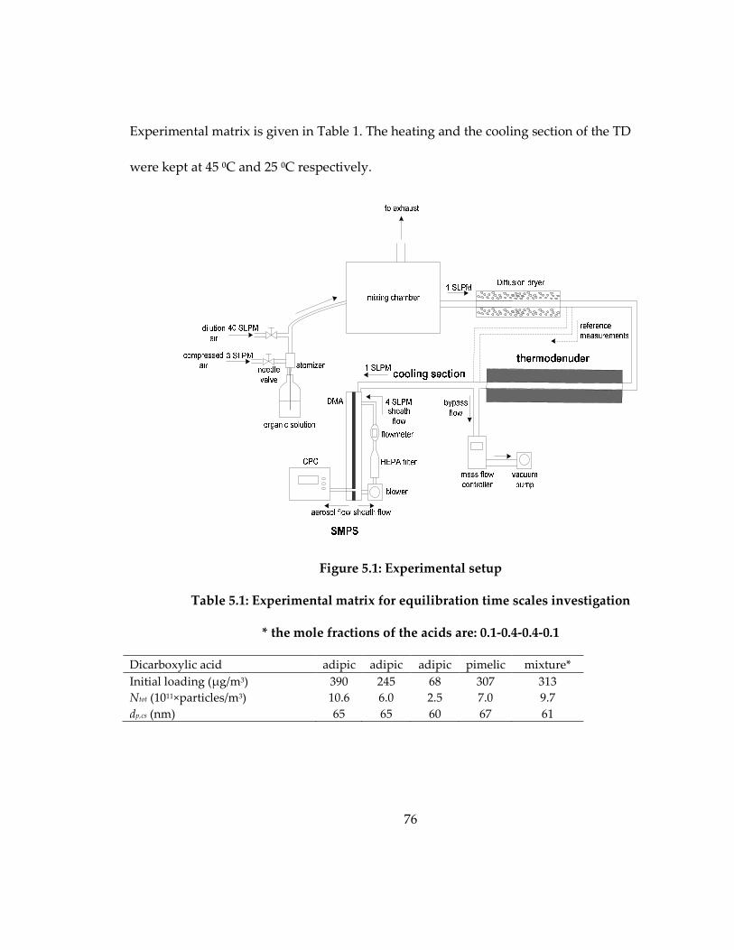
76

Experimental matrix is given in Table 1. The heating and the cooling section of the TD

were kept at 45 ⁰C and 25 ⁰C respectively.

Figure 5.1: Experimental setup

Table 5.1: Experimental matrix for equilibration time scales investigation

* the mole fractions of the acids are: 0.1-0.4-0.4-0.1

Dicarboxylic acid adipic adipic adipic pimelic mixture*

Initial loading (μg/m3) 390 245 68 307 313

Ntot (1011×particles/m3) 10.6 6.0 2.5 7.0 9.7

dp,cs (nm) 65 65 60 67 61

77

5.4 Reuslts and discussion

5.4.1 Effect of particle size distribution

Figure 5.2 shows ∆C and C*g of adipic acid aerosol at different residence times in

the TD for different initial particle size distributions. The results of numerical

simulations using the model described in section 5.2.1 are also shown. Equilibrium

corresponds to C*g = 1. It is evident that equilibration times are dependent on particle

size distributions – more specifically on the total particle length – as predicted by

equation (5.6). For aerosol size distributions relevant to laboratory studies, adipic acid

aerosol reaches equilibrium within a residence time typical for most TDs currently

employed. However, for size distributions relevant for ambient measurements,

equilibration requires residence times much larger than what is available with current

TD designs.

It should be noted that the asymptotic behavior exhibited by C*g as time

progresses demonstrates that the wall losses in the thermodenuder are negligible. If the

losses were significant, there would be no such asymptotic behavior, as the material will

be continuously stripped by the walls, resulting in an ever increasing ∆C. The excellent

agreement between the observations and the model, which assumes no wall losses in the

heated section, further supports this point.

78

5.4.2 Effect of the evaporation coefficient

As shown in section 5.2.2, equilibration times depend on the evaporation

coefficient (α) (i.e. F in equation 6)). To obtain agreement between model simulations

and experimental data in Figure 2, α of approximately 0.1 is required. This is consistent

with the value of α reported by Saleh et al. (2009) for adipic acid (0.08 ±0.02). To

illustrate the importance of this parameter, Figure 5.3 shows model simulations for

vapor build-up of adipic acid aerosol for different values of α. It is obvious that using

values of α greater than 0.1 over-predicts the observed SR, while values less than 0.1

under-predict the observations.

When TD measurements are performed at non-equilibrium conditions and the

volatility is calculated from evaporation kinetics model simulations, as suggested by

Riipinen et al. (2010) and Cappa (2010), the results strongly depend on α, which is often

unknown. Thus when α is unknown, it is critical that TDs are used in a manner such that

measurements are made under equilibrium conditions. However, as described in section

5.4.1, equilibrium cannot be achieved in the TD when performing ambient

measurements. The best approach pending developments in the state of the art, is to

interpret ambient TD measurements using kinetic models, as done in Cappa and

Jimenez (2010), while keeping in mind the substantial uncertainty due to unknown α, as

pointed out by those authors.

79

Figure 5.2: Measured and simulated particle mass change and dimensionless

vapor build-up profiles for adipic acid aerosol in a TD. Tin = 25 ⁰C and Tw = 40 ⁰C.

Squares & solid: C0 = 390 μg/m3, Ntot = 1012 particles/m3, dp,cs = 65 nm; diamonds &

broken: C0 = 245 μg/m3, Ntot = 6×1011 particles/m3, dp,cs = 65 nm; stars & dotted: C0 = 68

μg/m3, Ntot = 2.5×1011 particles/m3, dp,cs = 60 nm

0 5 10 15 20 25 30 350

0.2

0.4

0.6

0.8

1

residence time (s)

Cg*

0 5 10 15 20 25 30 35

5.3

10.5

15.8

21

26.3

∆C

(µ

g/m

3 )

80

Figure 5.3: Measured and simulated vapor build-up profiles for adipic acid

aerosol (C0 = 390 μg/m3, Ntot = 1012 particles/m3, dp,cs = 65 nm) in a TD. The simulations

were performed with α as a variable parameter as indicated in the Figure. Tin = 25 ⁰C

and Tw = 40 ⁰C.

5.4.3 Effect of thermodynamic properties and mixtur e complexity

To investigate the purported effect of Csat, we performed equilibration

experiments with pimelic acid, which has Csat(40 ⁰C) a factor of 3 greater than that of

adipic acid, and with a mixture of succinic, adipic, pimelic, and azelaic acids.

Experimental SR versus residence time for adipic acid, pimelic acid, and the dicarboxylic

acids mixture is shown in Figure 5.4 along with model predictions. Particle size

0 5 10 15 20 25 30 350

0.2

0.4

0.6

0.8

1

residence time (s)

Cg*

α = 1 α = 0.1

α = 0.05

α = 0.01

α = 0.5

81

distribution was held constant across the experiments to the extent possible. It is

apparent that the three model aerosols exhibited similar vapor build-up profiles, which

verifies the theoretical finding that equilibration time scales are neither a function of Csat

nor mixture complexity. For pimelic acid, α of approximately 0.25 was required for the

model to match experimental data, which is in agreement with the value reported by

Saleh et al. (2009) (0.24 ±0.04). For the dicarboxylic acids mixture, the effective α required

in the simulation was around 0.12, which is within the range of values of the

components.

It has been argued (Riipinen et al, 2010) that an aerosol with a large Csat needs

more time to achieve equilibrium than one with a small Csat because the former must

evaporate more than the latter to saturate the gas phase. However, this effect is

counterbalanced by the increased evaporation rate of the larger Csat aerosol (i.e. as given

by the Maxwell equation). The same applies to mixture complexity. Although in a

mixture the evaporation rate of each component is reduced by a factor of xi, the mole

fraction of component i in the mixture, relative to that of the pure compound, the

equilibrium concentration in the gas phase of component i is reduced by the same factor

according to Ceq,i = xi Csat,i. This analysis can be deduced directly from the non-

dimensional form of the vapor concentration rate equation (equation (5.6)).

82

Confusion over the role of Csat appears to stem from how some investigators

define equilibration. For example, Riipinen at al. (2010) define equilibration as the point

when the aerosol particles are within 1% or 10 nm of the equilibrium diameter deq,

whichever comes first. However, thermodynamic equilibrium is determined by the gas

concentration, not particle size, i.e. the problem is mass-based. The problem with the

size-based criterion can be observed by performing the following thought experiment.

Consider two aerosols with the same initial size (d0 = 200 nm) and concentration (C0 =

150 μg/m3), but different saturation concentrations at the TD temperature (Csat,1 = 50

μg/m3 and Csat,2 = 140 μg/m3). Assuming that Csat at T0 is much smaller than Csat at T(TD),

the final equilibration concentrations are Ceq,1 = C0 – Csat,1 = 100 μg/m3 and Ceq,2 = C0 – Csat,2

= 10 μg/m3. For spherical particles, the equilibrium diameters can be calculated from

, 1/3

6

( )eq

p eq

Cd

Nπρ= , where ρ is the particle density and N is the number concentration.

This gives dp,eq,1 = 175 nm and dp,eq,2 = 81 nm. Using the 1% or 10 nm equilibration

criterion, we get dp,1 = 185 nm and dp,2 = 91 nm, giving final concentrations C1 of 118

μg/m3 and C2 of 14 μg/m3. The saturation ratios for cases 1 and 2 can be calculated from

0 1,21,2

,1,2sat

C CSR

C

−= as 64% and 97% respectively. It is obvious that case 1 would be thought

to have reached equilibrium quite prematurely relative to case 2 in an evaporation

kinetics simulation, which would lead to the erroneous outcome that equilibrium at state

83

1 is achieved faster than state 2, eventually leading to the invalid conclusion that

equilibration time scales increase with increasing Csat.

Figure 5.4: Measured and simulated vapor build-up profiles. Squares & solid:

adipic acid, C0 = 390 μg/m3 and dcs = 65 nm; triangles & broken: pimelic acid, C0 = 307

μg/m3 and dcs = 67 nm; circles & dotted: succinic+adipic+pimelic+azelaic acid mixture,

C0 = 313 μg/m3 and dcs = 61 nm. Tin = 25 ⁰C and Tw = 40 ⁰C.

5.4.4 Effect of the equilibration parameter

The equilibration parameter derived in section 5.2.2 as ,/ 2r tot p in rt N d DFtτ π= can

be used semi-empirically to estimate the required residence time in a TD for a certain

aerosol to equilibrate. Figure 5.5 shows C*g plotted as a function of tr/τ for the

0 5 10 15 20 25 30 350

0.2

0.4

0.6

0.8

1

residence time (s)

Cg*

84

experimental data reported in Figure 5.2 and Figure 5.4. It can be seen in Figure 5.5 that

when plotted this way, the experimental data coalesce, as expected from the

dimensional analysis which indicated that the process is governed by tr/τ. The model

simulations shown in Figure 5.2 and Figure 5.4 also collapse to approximately the same

line when plotted as a function of tr/τ, and are presented by a single solid line in Figure

5.5. Using C*g = 0.95 as the equilibration criterion, the measured and simulated aerosols

approach equilibrium for tr/τ ≈ 5. Because the derivation of τ is based on the assumption

that the change in particle size upon evaporation is small, the value of tr/τ required for

equilibration increases with deviation from the assumption. However, τ is still a

valuable parameter to estimate equilibration times for most practical cases. Model

simulations showed that for relative aerosol mass change (∆C/C0) between 10% and 90%,

tr/τ between 5 and 9 was required for equilibration. tr/τ > 9 can thus be used to define

equilibration in TDs. For an aerosol with a certain size distribution and kinetic

properties, the required residence time to achieve equilibrium can thus be estimated,

and the TD can be designed accordingly.

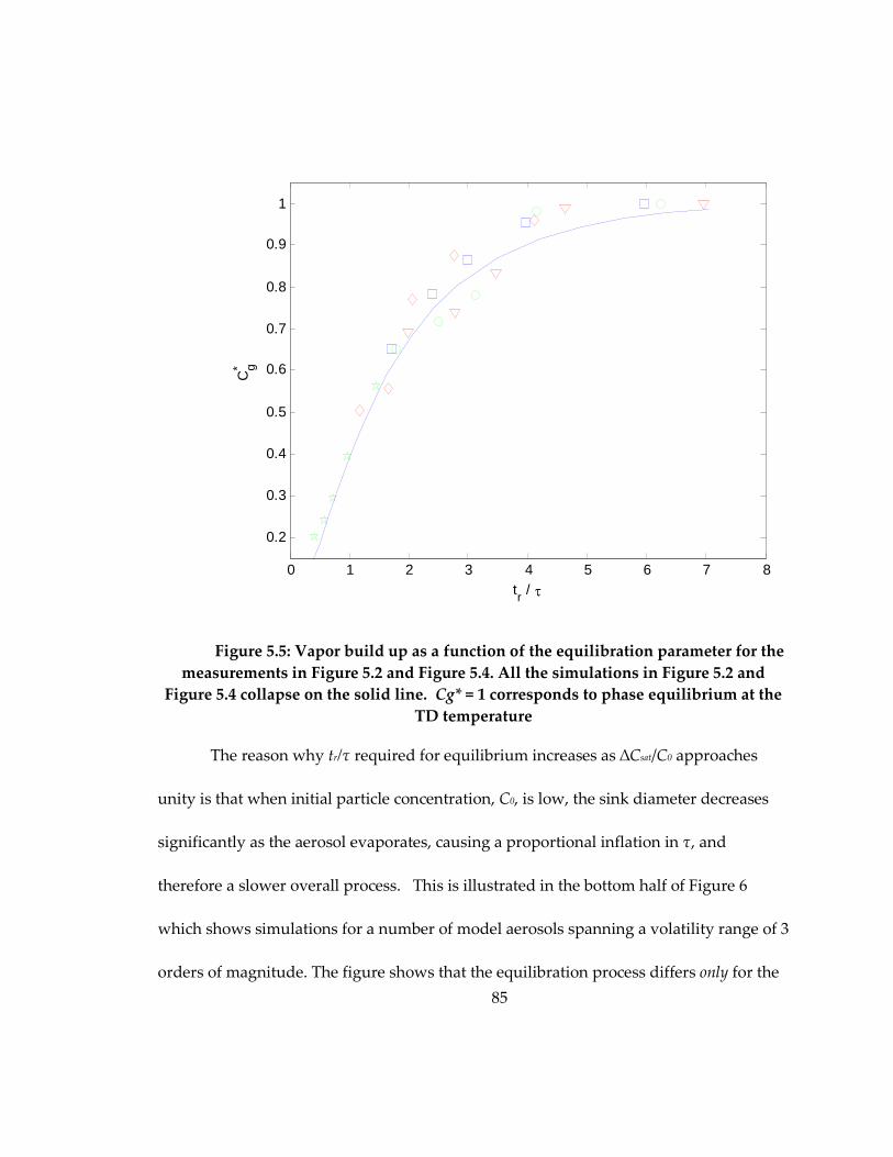
85

Figure 5.5: Vapor build up as a function of the equilibration parameter for the

measurements in Figure 5.2 and Figure 5.4. All the simulations in Figure 5.2 and

Figure 5.4 collapse on the solid line. Cg* = 1 corresponds to phase equilibrium at the

TD temperature

The reason why tr/τ required for equilibrium increases as ∆Csat/C0 approaches

unity is that when initial particle concentration, C0, is low, the sink diameter decreases

significantly as the aerosol evaporates, causing a proportional inflation in τ, and

therefore a slower overall process. This is illustrated in the bottom half of Figure 6

which shows simulations for a number of model aerosols spanning a volatility range of 3

orders of magnitude. The figure shows that the equilibration process differs only for the

0 1 2 3 4 5 6 7 8

0.2

0.3

0.4

0.5

0.6

0.7

0.8

0.9

1

tr / τ

Cg*

86

model aerosols which are relatively lean in the particle phase (i.e. the curves

corresponding to ∆Csat/C0 of 0.5 and 0.8); put another way, as long as the aerosol has

ample material in the particle phase relative to what is needed to saturate the vapor

phase, equilibration time will be unaffected by volatility. This is more poignantly

illustrated in the top half of Figure 6, where the same data is plotted versus non-

dimensional time, tr/τ(t), in which τ(t) is calculated using d(t). It can be seen that all the

curves, including those with large values of ∆Csat/C0, collapse onto a single line,

illustrating simply what is demonstrated in equation 5.5, namely that under all

circumstances for which equilibration is possible τ governs the process.

When the value of α is unknown, which is often the case, τ can be calculated

based on an assumed α and used to obtain a first order approximation of the required

residence time. Experimental variation of TD residence time, as described in section 5.3,

is then needed to verify that the aerosol has equilibrated. It should be noted that

equilibration is possible to achieve only when C0 > Csat(TTD) – Csat(T0), otherwise the

aerosol particles would evaporate completely and equilibrium will not be attained

regardless of the value of tr/τ.

87

Figure 5.6: Simulated normalized vapor build-up profiles in a TD as a function

of residence time (bottom x-axis and left y-axis) and time-dependent equilibration

parameter (upper x-axis and right y-axis). T0 = 25 ⁰C; TTD = 40 ⁰C; ∆H = 100 kJ/mol; Co =

230 μg/m3; red: Csat = 0.14 μg/m3, ∆Csat/C0 = 5×10-4; green: Csat = 1.4 μg/m3, ∆Csat/C0 = 5×10-

3; blue: Csat = 14 μg/m3, ∆Csat/C0 = 0.05; cyan: Csat = 140 μg/m3, ∆Csat/C0 = 0.5; yellow: Csat =

225 μg/m3, ∆Csat/C0 = 0.8

5.4.5 Re-condensation in the cooling section

As described in section 5.2.3, the rate at which vapor re-condenses on the aerosol

particles relative to the mass transfer rate to the walls is represented by the

dimensionless coupling number ,2 tot p in t

m

N d FDdCn

hπ= . Figure 5.7 shows maximum

theoretical re-condensation fraction (RF) as a function of Cn for cooling sections with no

0 10 20 30 40 50 60

0.2

0.4

0.6

0.8

1

residence time (s)

Cg*

0 2 4 6 8 10 12

0

0.2

0.4

0.6

0.8

1

tr / τ(t)

Cg*

88

AC denuder. RF is defined as the ratio of the amount of vapor that re-condenses on the

aerosol particles when they achieve equilibrium in the cooling section to the amount of

vapor that has evaporated from the particles in the TD. RF is maximum re-condensation

fraction because if the aerosol is sampled from the cooling section before it achieves

equilibrium, re-condensation fraction would be less than RF. Different Cn values were

generated by randomly varying aerosol size distribution and/or cooling section

geometry. As expected, re-condensation becomes more important with increasing Cn.

Values of Cn < 0.7 mark the region where re-condensation is not significant (< 10%). We

should note that for ambient measurements and the vast majority of laboratory

experiments, Cn is well below 0.7.

For most practical cases, incorporating an AC denuder has no significant effect.

The reason is that value of Cg entering the cooling section is usually much greater than

Csat(Tw), which renders the concentration gradient between the gas phase and the cooling

section walls (Cg – 0) with an AC denuder very close to the case with no AC denuder (Cg

- Csat(Tw)). To illustrate, we have performed experiments with cooling sections with and

without an AC denuder. The initial and final mass concentrations – downstream of the

heating and cooling sections of the TD, respectively – for the cooling section

configurations described in section 5.3 are given in Table 2. As shown in the table, there

was no significant difference in the final mass concentration across the 4 configurations

89

for both model aerosols, which shows that the AC denuder had no observable effect in

our experiments.

Figure 5.7: Maximum re-condensation fraction as a function of Cn

While harmless at short residence times, an AC denuder might become

disadvantageous at long residence times, because the aerosol never achieves

equilibrium. The AC denuder will continue to strip the vapor from the gas phase

causing the aerosol particles to evaporate, leading to a bias in the measurement. Figure

5.8 shows theoretical RF for Cn of 0.5, for cases with and without an AC denuder. It is

10-2

10-1

100

101

102

0

10

20

30

40

50

60

70

Cn

RF

(%

)

90

obvious that with an AC denuder the aerosol particles will continue evaporating until

they completely disappear.

Figure 5.8: Maximum re-condensation fraction as a function of residence time

in the cooling section with and without an AC denuder for Cn = 0.5. Negative RF

indicates net evaporation of the aerosol relative to its state at the entrance of the

heated TD.

0 5 10 15 20 25 30-35

-30

-25

-20

-15

-10

-5

0

5

10

residence time in the cooling section (s)

RF

(%

)

without AC denuder

with AC denuder

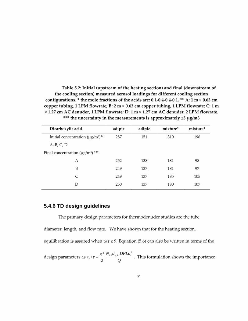
91

Table 5.2: Initial (upstream of the heating section) and final (downstream of

the cooling section) measured aerosol loadings for different cooling section

configurations. * the mole fractions of the acids are: 0.1-0.4-0.4-0.1. ** A: 1 m × 0.63 cm

copper tubing, 1 LPM flowrate; B: 2 m × 0.63 cm copper tubing, 1 LPM flowrate; C: 1 m

× 1.27 cm AC denuder, 1 LPM flowrate; D: 1 m × 1.27 cm AC denuder, 2 LPM flowrate.

*** the uncertainty in the measurements is approximately ±5 μg/m3

Dicarboxylic acid adipic adipic mixture* mixture*

Initial concentration (μg/m3)**

A, B, C, D

287 151 310 196

Final concentration (μg/m3) ***

A 252 138 181 98

B 249 137 181 97

C 249 137 185 105

D 250 137 180 107

5.4.6 TD design guidelines

The primary design parameters for thermodenuder studies are the tube

diameter, length, and flow rate. We have shown that for the heating section,

equilibration is assured when tr/τ ≥ 9. Equation (5.6) can also be written in terms of the

design parameters as 22

,/2

tot p in tr

N d DFLdt

Q

πτ = . This formulation shows the importance

92

of tube diameter; tr/τ scales with the square of the TD diameter and linearly with TD

length.

Having achieved equilibrium in the heating section, the role of the cooling

section is to bring the aerosol to the temperature of the sizing instrument with as little

change as possible in the particle size distribution. To the extent possible, condensation

of the vapor phase should occur preferentially on the tube wall rather than on the

particles flowing through it. For the problem at hand, cooling sections should be

designed to minimize Cn. We have shown that for Cn < 0.7, re-condensation is not

significant. It can be readily shown that for a laminar flow characterized by a constant

Sherwood number, Cn scales with the square of the tube diameter. Thus to minimize re-

condensation on the particle phase, the cooling section should have a small diameter, in

contrast to the heating section.

5.5 Conclusions

Heat and mass transport and aerosol evaporation/growth kinetics in

thermodenuders were studied both theoretically and experimentally. Numerical

simulations of the evolution of aerosols in a TD using a plug flow computational model

exhibited excellent agreement with experimental measurements performed with pure

and mixed dicarboxylic acid aerosols.

93

For size distributions typical for laboratory experiments, we found that pure and

mixed dicarboxylic acid aerosols approach equilibrium in TDs within residence times on

the order of 10 seconds. However, for size distributions relevant to ambient aerosols,

equilibration cannot be achieved within residence times available with current TD

designs.

We have shown through dimensional analysis and empirical measurements that

contrary to common assumption, equilibration kinetics in a TD are not affected by

volatility. Rather, equilibration time is only a function of aerosol size and number

concentration, evaporation coefficient, and vapor diffusivity, as described by a time

constant τ. Experiments and model simulations showed that tr/τ = 9 marks the onset of

equilibration, which can be used to aid TD design to ensure equilibration.

The problem of re-condensation in the cooling section can be characterized by

the coupling number (Cn). Cn represents the ratio of the rate aerosol particles scavenge

vapor from the gas phase to the rate vapor is transported to the walls of the cooling

section. To minimize re-condensation, Cn should be less than 0.7, which can be achieved

by minimizing the diameter of the cooling section. We showed both experimentally and

by simulation that re-condensation is not important for aerosol size distributions

relevant to laboratory studies and ambient measurements. We also showed that for short

residence times, using an AC denuder in the cooling section has no effect. Further, an

94

AC denuder might be disadvantageous if it has a residence time long enough to distill

the vapor from the gas phase which causes further evaporation of the aerosol particles.

AC denuders should thus be avoided in cooling section of TDs.

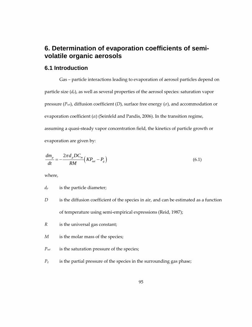
95

6. Determination of evaporation coefficients of sem i-volatile organic aerosols

6.1 Introduction

Gas – particle interactions leading to evaporation of aerosol particles depend on

particle size (dp), as well as several properties of the aerosol species: saturation vapor

pressure (Psat), diffusion coefficient (D), surface free energy (σ), and accommodation or

evaporation coefficient (α) (Seinfeld and Pandis, 2006). In the transition regime,

assuming a quasi-steady vapor concentration field, the kinetics of particle growth or

evaporation are given by:

( )2π= − −p p m

sat g

dm d DCKP P

dt RM (6.1)

where,

dp is the particle diameter;

D is the diffusion coefficient of the species in air, and can be estimated as a function

of temperature using semi-empirical expressions (Reid, 1987);

R is the universal gas constant;

M is the molar mass of the species;

Psat is the saturation pressure of the species;

Pg is the partial pressure of the species in the surrounding gas phase;

96

K is Kelvin correction factor due to curvature, and is given by 4

expp p

MK

Td

σρ

=

,

where pρ is the density of the particle, T is the temperature and is the surface

free energy;

Cm is Fuchs-Sutugin correction factor for non-continuum effects, and is given by

(Fuchs and Sutugin, 1971): 1

1 0.3773 1.33 (1 ) /m

KnC

Kn Kn Kn α+

=+ + +

, where α is the

evaporation coefficient.

The evaporation coefficient is generally defined as the ratio of the molecular flux

desorbed from a particle to the maximum theoretical flux predicted by kinetic theory.

At equilibrium, the inbound and outbound molecular fluxes from a particle are equal,

and thus the maximum rate at which vapor molecules can be desorbed is taken as the

maximum rate they can be added to the particle surface during condensation. This

maximum is given by the frequency at which vapor molecules collide with the surface

(i.e. assuming every collision results in a molecule “sticking”), assuming inbound

molecules carry a Maxwell-Boltzmann velocity distribution and exist in the vapor phase

at a concentration corresponding to saturation conditions.

In the free molecular regime, the relation between maximum theoretical

evaporation flux, molecular velocity, and concentration (expressed as pressure assuming

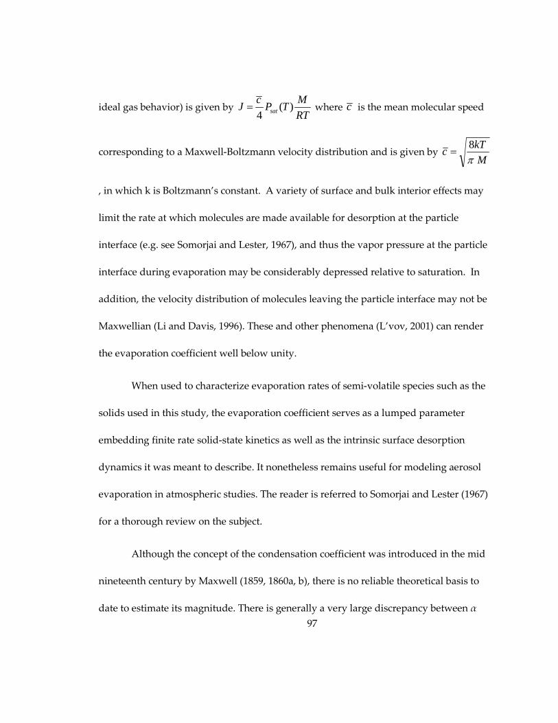
97

ideal gas behavior) is given by ( )4 sat

c MJ P T

RT= where c is the mean molecular speed

corresponding to a Maxwell-Boltzmann velocity distribution and is given by M

kTc

π8

=

, in which k is Boltzmann’s constant. A variety of surface and bulk interior effects may

limit the rate at which molecules are made available for desorption at the particle

interface (e.g. see Somorjai and Lester, 1967), and thus the vapor pressure at the particle

interface during evaporation may be considerably depressed relative to saturation. In

addition, the velocity distribution of molecules leaving the particle interface may not be

Maxwellian (Li and Davis, 1996). These and other phenomena (L’vov, 2001) can render

the evaporation coefficient well below unity.

When used to characterize evaporation rates of semi-volatile species such as the

solids used in this study, the evaporation coefficient serves as a lumped parameter

embedding finite rate solid-state kinetics as well as the intrinsic surface desorption

dynamics it was meant to describe. It nonetheless remains useful for modeling aerosol

evaporation in atmospheric studies. The reader is referred to Somorjai and Lester (1967)

for a thorough review on the subject.

Although the concept of the condensation coefficient was introduced in the mid

nineteenth century by Maxwell (1859, 1860a, b), there is no reliable theoretical basis to

date to estimate its magnitude. There is generally a very large discrepancy between α

98

values obtained by molecular dynamics (MD) simulations and experiments (Davis,

2006). α of different compounds has been investigated using various experimental

techniques. For an extensive review on the available techniques, the reader is referred to

Davis (2006). α of water has received much attention because of its importance in cloud

microphysics. Values in the range of 0.04 to 1 have been reported, with more recent

measurements providing values closer to 1 (Li et al., 2001; Voigtlander et al., 2007;

Winkler et al., 2006; Pruppacher and Klett, 1996). α values for a number of other species

have also been reported. Sulfuric acid was reported to have α of approximately 0.65

(Poschl et al., 1998). Values of 0.73 and 0.79 were observed for condensation of sulfuric

acid onto ammonium sulfate and sodium chloride aerosols (Jefferson et al., 1997). α close

to 1 was reported for condensation of ammonia onto droplets of 15-65% sulfuric acid

solution (Hanson and Kosciuch, 2007). Values around 0.11 were reported for nitric acid

condensing to sulfuric acid solutions (Xue et al., 2005). Ammonium nitrate was reported

to exhibit α values of 0.5-0.8 in pure form (Dassios and Pandis, 1999) and of 0.25, if

coated with dioctyl phthalate (Cruz et al., 2000).

There is paucity of data on α of organic compounds relevant to organic ambient

aerosols. Li and Davis (1996) found α close to unity for dibutyl phthalate droplets

evaporating in an electrodynamic balance. Riipinen et al. (2006) also reported α close to

unity for succinic acid in aqueous solution. Their findings were based on a comparison

99

between Tandem Differential Mobility Analysis (TDMA) experiments and simulations

performed with an evaporation / condensation model (BCOND). On the other hand,

Stanier et al. (2007) estimated that α values of less than 0.1 are required to match their

evaporation simulations using a basis-set approximation with TDMA measurements for

SOA generated in a smog chamber by α-pinene ozonolysis. Another smog chamber

study by Bowman et al. (1997) estimated α between 0.1 and 1 for aerosol resulting from

m-xylene/NOx experiments. As noted above, the evaporation coefficient may embed a

number of processes other than surface desorption, and, especially in the case of

complex aerosols such as SOA, these processes can be rate-limiting, resulting in low

values for α. Cruz and Pandis (2000) reported α values of greater than 0.2 for

condensation of dioctyl phthalate and glutaric acid on inorganic and organic particles.

6.2 The IV-TDMA method

A major difficulty associated with estimating α in the transition regime is that its

effect on particle evaporation or condensation rate overlaps with that of Psat and σ, as

evident in equation (6.1). In this study, we demonstrate a novel method, dubbed

integrated volume-tandem differential mobility analysis (IV-TDMA), to separate the

effects of these variables, allowing each α and σ to be determined by a single-parameter

least-squares technique. With this technique, the traditional Tandem Differential

Mobility Analyzer (TDMA)-thermodenuder approach is complemented with

100

measurements of aerosol vapor pressure under saturated conditions using the

Integrated Volume Method (IVM, Saleh et al, 2008). The IVM relates changes in total

particle volume as an aerosol passes from one equilibrium state to another, to vapor

pressure at a given temperature using the Clausius-Clapeyron equation. Once the vapor

pressure is determined, TDMA-thermodenuder experiments are performed to

characterize evaporation kinetics. The latter are first performed for particle sizes at

which the curvature effects are negligible (200-500 nm), allowing for single-parameter

optimization of the evaporation coefficient while constraining the surface free energy.

Having obtained the evaporation coefficient, measurements are repeated for smaller

particle sizes (100-200 nm) for which curvature effects are prominent, and single-

parameter optimization is used to obtain the surface free energy. Thus, the main three

parameters that govern aerosol evaporation in TDMA experiments, namely saturation

pressure, surface free energy and evaporation coefficient are decoupled. We illustrate

the IV-TDMA technique by applying it to C-4, -6, and -7 dicarboxylic acids, namely

succinic acid, adipic acid, and pimelic acid, which are pertinent to ambient / atmospheric

OA (Grosjean et al., 1978; Sempere and Kawamura, 1994).

6.2.1 The IVM

The IVM was described in detail in Chapter 2. Here, we just reiterate the main

advantage of the IVM, which is that the aerosol is investigated at equilibrium states,

101

excluding kinetics from the analysis. Thus, the knowledge of α is not required to

estimate Psat.

6.2.2 The TDMA method

In TDMA, quasi-monodisperse aerosol is heated in a thermodenuder and the size

change due to evaporation is measured. As opposed to the IVM, the aerosol in TDMA is

required to be as far from equilibrium as possible, such that the concentration of the

vapor of the aerosol species in the gas phase is negligible compared to the saturation

concentration. The particle evaporation kinetics equation (equation (6.1)) is thus

simplified to:

2π= −p p m satdm d DC KP

dt RM (6.2)

We note that the energy equation of the aerosol particles can be dropped because

the thermal inertia of the aerosol particles and the latent heat effects are negligible. This

was verified by comparison with a coupled heat-mass transfer model for aerosol

evaporation/condensation in tubular flow (Saleh and Shihadeh, 2007).

In the coupled IV-TDMA method, parameters in equation (6.2) are obtained as

follows:

• Psat,0 is calculated using the IVM. Psat at any temperature can be calculated with

the knowledge of ∆H using Clausius-Clapeyron equation (equation (2.4)).

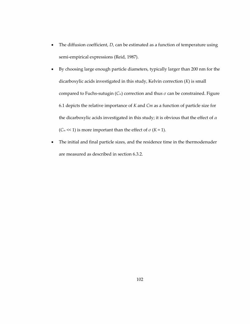
102

• The diffusion coefficient, D, can be estimated as a function of temperature using

semi-empirical expressions (Reid, 1987).

• By choosing large enough particle diameters, typically larger than 200 nm for the

dicarboxylic acids investigated in this study, Kelvin correction (K) is small

compared to Fuchs-sutugin (Cm) correction and thus σ can be constrained. Figure

6.1 depicts the relative importance of K and Cm as a function of particle size for

the dicarboxylic acids investigated in this study; it is obvious that the effect of α

(Cm << 1) is more important than the effect of σ (K ≈ 1).

• The initial and final particle sizes, and the residence time in the thermodenuder

are measured as described in section 6.3.2.

103

Figure 6.1: Relative importance of Fuchs-Sutugin correction (0 < Cm < 1 ) and

Kelvin effect (K > 1) for 100 nm – 600 nm particles at 298 K

The only unknown remaining in equation (6.2) is α. Equation (6.2) is numerically

integrated using MATLAB packaged ODE solver (ODE23) for a range of α values.

single-parameter least squares optimization is performed to obtain the best value of α

that produces a set of initial – final (evaporated) pairs of particle sizes.

Having estimated α, we apply the TDMA for particle sizes in the range 100 nm –

200 nm, where Kelvin effect is prominent, and equation (6.5) is optimized for σ.

100 200 300 400 500 6000

0.2

0.4

0.6

0.8

1

1.2

1.4

1.6

particle diameter (nm)

Cm ,

K

Pimelic acidAdipic acidSuccinic acid

Cm

K

104


6.3.1 Experimental setup and procedure

The experimental setup and procedure for IVM was described in details in

Chapter 2.

A schematic of the TDMA experimental setup is given in Figure 6.2. Dry

polydisperse organic aerosol is produced in a similar fashion as in the IVM experiments,

and a quasi-monodisperse fraction is selected by a Differential Mobility Analyzer (DMA,

TSI model 3071). The monodisperse flow is then rapidly pre-heated and diluted prior to

entering the thermodenuder. This step is needed to simplify data interpretation (see

section 6.2.2) and is achieved in the following way. Prior to the thermodenuder, the flow

is split into a second line which passes a HEPA filter and then an inline resistance heater

as illustrated in Figure 6.2. The filtered and preheated air is then returned to a point

right before the split, forming a loop. The air flow in the loop is maintained at 8 SLPM

using an in-line pump. The temperature of the mixed streams is monitored using an

RTD, and a PID controller is used to maintain a set temperature at the outlet of the inline

heater. The extraction line upstream of the HEPA filter in the pre-heating loop is 0.5 m

long (not shown to scale in Figure 6.2) to allow the aerosol to cool to room temperature;

otherwise, evaporation from the particles accumulated in the HEPA filter would cause

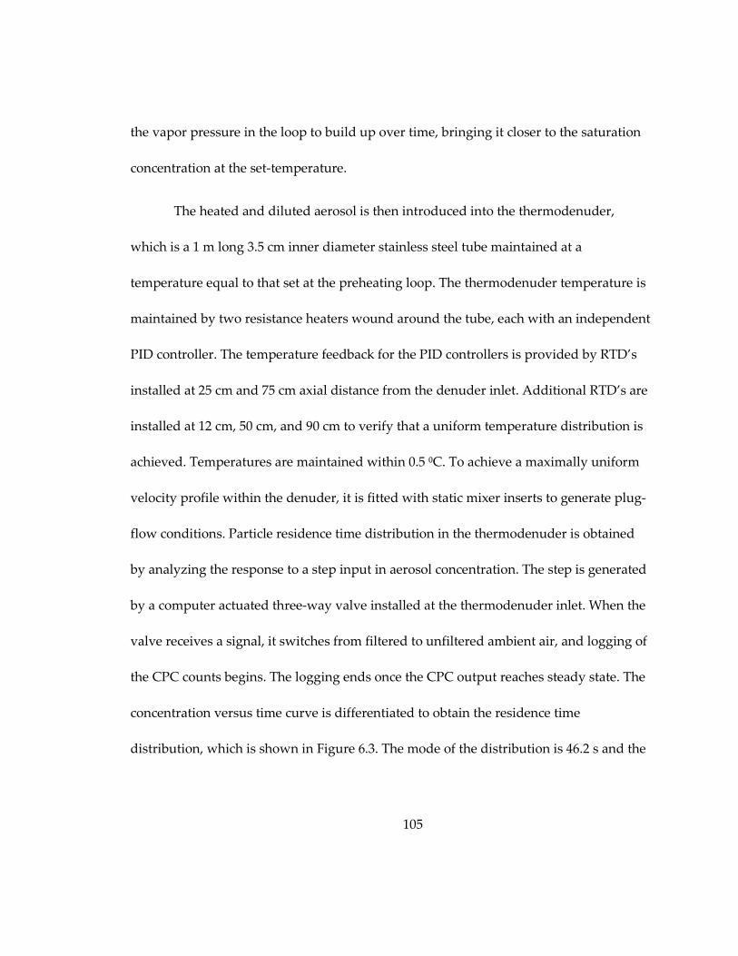
105

the vapor pressure in the loop to build up over time, bringing it closer to the saturation

concentration at the set-temperature.

The heated and diluted aerosol is then introduced into the thermodenuder,

which is a 1 m long 3.5 cm inner diameter stainless steel tube maintained at a

temperature equal to that set at the preheating loop. The thermodenuder temperature is

maintained by two resistance heaters wound around the tube, each with an independent

PID controller. The temperature feedback for the PID controllers is provided by RTD’s

installed at 25 cm and 75 cm axial distance from the denuder inlet. Additional RTD’s are

installed at 12 cm, 50 cm, and 90 cm to verify that a uniform temperature distribution is

achieved. Temperatures are maintained within 0.5 ⁰C. To achieve a maximally uniform

velocity profile within the denuder, it is fitted with static mixer inserts to generate plug-

flow conditions. Particle residence time distribution in the thermodenuder is obtained

by analyzing the response to a step input in aerosol concentration. The step is generated

by a computer actuated three-way valve installed at the thermodenuder inlet. When the

valve receives a signal, it switches from filtered to unfiltered ambient air, and logging of

the CPC counts begins. The logging ends once the CPC output reaches steady state. The

concentration versus time curve is differentiated to obtain the residence time

distribution, which is shown in Figure 6.3. The mode of the distribution is 46.2 s and the

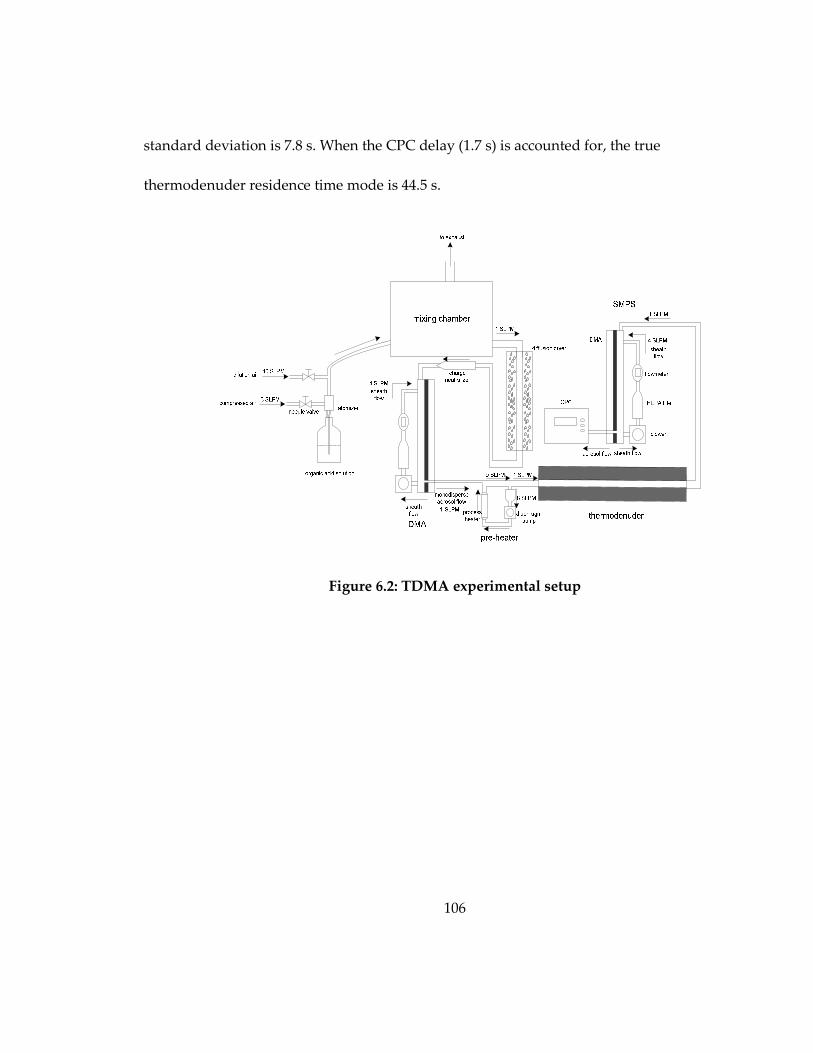
106

standard deviation is 7.8 s. When the CPC delay (1.7 s) is accounted for, the true

thermodenuder residence time mode is 44.5 s.

Figure 6.2: TDMA experimental setup

107

Figure 6.3: Residence time distribution in the thermodenuder

The final particle size at the exit of the thermodenuder is measured using an

SMPS. To verify that we have vapor free conditions in the gas phase, as required in

TDMA experiments (section 6.2.2), we measure the initial (Cinitial) and the final (Cfinal) total

aerosol particle mass concentrations. We compare the difference between these two

concentrations (which is the vapor concentration released to the gas phase) to the species

saturation concentration at the experimental temperature (Csat,T). The ratio (Cinitial - Cfinal) /

Csat,T was always less than 1%, which is very small compared to the 30% uncertainty in

Psat (see section 6.3.2).

0 20 40 60 80 100 120 140 160

0

20

40

60

80

100

120

140

160

time (s)

dC/d

t (#/

cm3 s)

108

6.3.2 Uncertainty analysis

Uncertainty of the IV-TDMA measurements is associated with the following

parameters:

• Psat obtained by IVM: the uncertainty is approximately 30% (Saleh et al., 2008).

• Particle size: the uncertainty in particle size measurements using a DMA is

estimated to be 3% (Kinney and David, 1991).

• Residence time in the thermodenuder: the uncertainty is estimated to be the

standard deviation of the residence time distribution (7.8 s).

• For surface free energy estimation, we also consider the uncertainty in the

estimated evaporation coefficients.

To assess the propagation of uncertainty in our model, we use a Monte-Carlo

approach with 100 simulations, each with perturbed values of the above parameters

defined as:

φ= +perturbedXX X u (6.3)

where X is the mean value of one of the parameters (saturation pressure, particle

diameter, residence time, or accommodation coefficient), Xu is the corresponding

uncertainty, and φ is a random variable drawn from a normal distribution with mean of

0 and standard deviation of 1. Results from the simulations are used to calculate mean

values and uncertainties in the evaporation coefficients and surface free energies.

109


6.4.1 Evaporation coefficients and surface free ene rgies

Decrease in particle size due to evaporation in TDMA experiments is shown in

Figure 6.4 for succinic, adipic, and pimelic acid. Data points on the right side of the plots

(larger diameters) are used for α determination, and points on the left side (smaller

diameters) are used for σ determination. The set-temperature at which each experiment

was performed was found by trial and error to produce measurable size changes for the

residence time in the thermodenuder. Set-temperatures for different experiments are

given in Table 6.1. The initial and final particle sizes for each acid are listed in Table 6.2.

Figure 6.4

100 150 200 250 300 350 4000.5

0.55

0.6

0.65

0.7

0.75

0.8

0.85

0.9

0.95

dinitial

(nm)

d final /

d initi

al

(a)

110


100 150 200 250 300 350 4000.72

0.74

0.76

0.78

0.8

0.82

0.84

0.86

0.88

0.9

dinitial (nm)

d final /

d initi

al

(b)

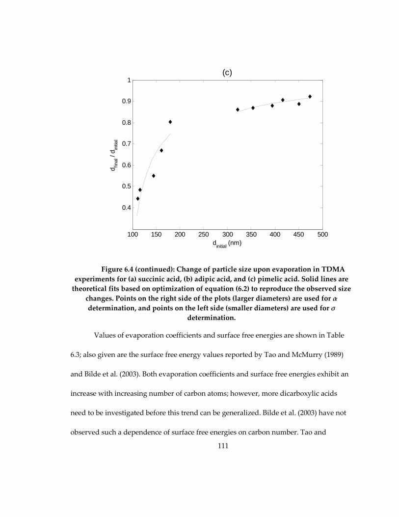
111

Figure 6.4 (continued): Change of particle size upon evaporation in TDMA

experiments for (a) succinic acid, (b) adipic acid, and (c) pimelic acid. Solid lines are

theoretical fits based on optimization of equation (6.2) to reproduce the observed size

changes. Points on the right side of the plots (larger diameters) are used for α

determination, and points on the left side (smaller diameters) are used for σ

determination.

Values of evaporation coefficients and surface free energies are shown in Table

6.3; also given are the surface free energy values reported by Tao and McMurry (1989)

and Bilde et al. (2003). Both evaporation coefficients and surface free energies exhibit an

increase with increasing number of carbon atoms; however, more dicarboxylic acids

need to be investigated before this trend can be generalized. Bilde et al. (2003) have not

observed such a dependence of surface free energies on carbon number. Tao and

100 150 200 250 300 350 400 450 500

0.4

0.5

0.6

0.7

0.8

0.9

1

dinitial

(nm)

d final /

d initi

al

(c)

112

McMurry (1989) reported virtually identical surface energies for glutaric and adipic

acids with the latter having slightly lower surface free energy. However, they observed a

clear increase in surface free energies with increasing carbon number in C14-C18

monocarboxilic acids.

Table 6.1: Thermodenuder set-temperatures for TDMA experiments

Investigated property Acid Thermodenuder set-

temperature

α Succinic

Adipic

Pimelic

40 ⁰C

50 ⁰C

37 ⁰C

σ Succinic

Adipic

Pimelic

40 ⁰C

45 ⁰C

35 ⁰C

Evaporation coefficients are significantly less than unity for the three

dicarboxylic acids investigated in this study. While our experiments were done with

pure substances, these results are in line with the findings of Stanier et al. (2007) and

Bowmann et al. (1997) on evaporation coefficients associated with SOA generated in

smog chamber studies, indicating evaporation coefficients smaller than one.

Table 6.2: Initial and final particle sizes (nm) for TDMA experiments

succinic acid adipic acid pimelic acid

113

initial size final size initial size final size intial size final size

α

determination

220

224

249

265

280

395

320

356

391

187

187

211

227

249

268

288

302

356

252

272

285

314

326

399

201

218

238

263

288

346

322

354

394

417

451

473

277

308

347

378

400

437

σ

determination

112

118

138

157

167

65

69

84

97

114

115

127

155

169

189

87

99

125

137

157

112

116

144

161

180

50

56

79

108

145

To investigate the validity of our assumption that the effects of α and σ are

decoupled, we first perform α optimization assuming no Kelvin effect. Using the

calculated α value, we optimize for σ, and then use the calculated σ value to re-calculate

α. For succinic acid and adipic acid, the values obtained for α are the same in both cases

(with and without Kelvin effect), thus confirming the decoupling. However, for pimelic

acid, we observed some σ-dependence in calculating α, and we had to perform three

iterations of α and σ optimizations for convergence. The reason for this dependence is

that σ and α for pimelic acid are relatively large, and thus Kelvin and Fuchs-Sutugin

corrections are relatively close, as can be inferred from Figure 6.1.

Table 6.3: Evaporation coefficients and surface free energies of the

dicarboxylic acids

Property Acid This work Tao and McMurry Bilde et al. (2003)

114

(1989)

α Succinic

Adipic

Pimelic

0.07 (± 0.02)

0.08 (± 0.02)

0.24 (± 0.04)

σ (J/m2) Succinic

Adipic

Pimelic

0.15 (± 0.07)

0.17 (± 0.12)

0.23 (± 0.08)

0.28

0.125

0.06

0.08

6.4.2 Temperature dependence of the evaporation coe fficient

The values of α reported in Table 6.3 for the dicarboxylic acids were obtained at

temperatures 15 ⁰C – 20 ⁰C above the ambient (Table 6.1). The reason, as described in

section 6.3.1, is that if the experiments were to be performed at temperatures close to the

ambient, impractically long residence times would be required in the thermodenuder to

achieve measurable size changes. To assure that the measured α values are

representative for ambient conditions, we investigated the temperature dependence of

α. It should be noted that the temperature-dependence of α is a highly debatable issue,

with some studies observing no dependence (Winkler et al., 2006) and others reporting it

(Davidovits et al., 2006).

TDMA experiments were performed for each compound at 4 different

temperatures. The flowrate in the thermodenuder was adjusted for each set-temperature

to obtain size changes which are measurable, but not too large so that the Kelvin effect is

115

constrained (see section 6.3.1). The set-temperatures and corresponding flowrates for

each dicarboxylic acid are given in Table 6.4.

Measured α as a function of temperature is shown in Figure 6.5. Over a

temperature range of 20 ⁰C, adipic acid and succinic acid exhibit no observed

temperature dependence, while pimelic acid exhibits a weak negative dependence,

which is, however, within the uncertainty of the measurements. These results indicate

that the difference in α between experimental and ambient temperature, if any, is small,

and thus the values obtained in this study are representative for ambient conditions.

Table 6.4: Flowrates in thermodenuder for each set-temperature for α

determination TDMA measurements

dicarboxylic acid set-temperature (⁰C) set-flowrate (LPM)

succinic 40

45

50

55

1

4

5

8

adipic 40

50

55

60

0.5

1

5

7

pimelic 37

45

50

55

1

5

9

11

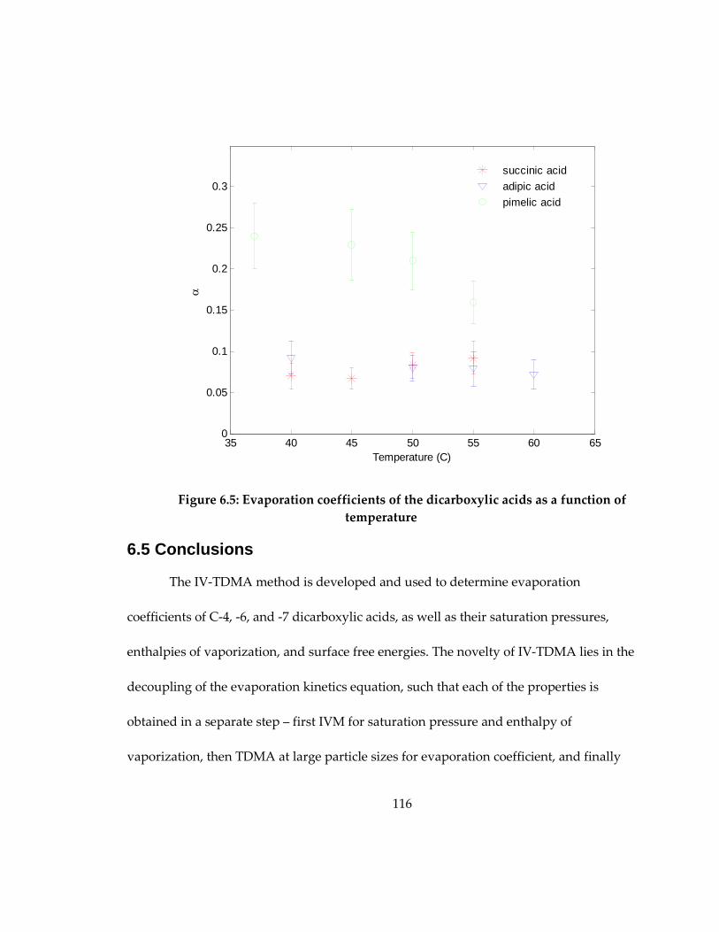
116

Figure 6.5: Evaporation coefficients of the dicarboxylic acids as a function of

temperature

6.5 Conclusions

The IV-TDMA method is developed and used to determine evaporation

coefficients of C-4, -6, and -7 dicarboxylic acids, as well as their saturation pressures,

enthalpies of vaporization, and surface free energies. The novelty of IV-TDMA lies in the

decoupling of the evaporation kinetics equation, such that each of the properties is

obtained in a separate step – first IVM for saturation pressure and enthalpy of

vaporization, then TDMA at large particle sizes for evaporation coefficient, and finally

35 40 45 50 55 60 650

0.05

0.1

0.15

0.2

0.25

0.3

Temperature (C)

α

succinic acid

adipic acid

pimelic acid

117

TDMA at small sizes for surface free energy – rather than relying on multi-dimensional

optimization.

The evaporation coefficients obtained in this study for the three dicarboxylic

acids are significantly less than one. This highlights the importance of investigation of

evaporation coefficients of ambient/atmospheric semi-volatile organic aerosols to

improve the understanding of their phase change kinetics.

118

7. Conclusions

This dissertation presents novel experimental approaches for determination of

thermodynamic and kinetic properties of semi-volatile organic aerosols. Two

experimental techniques were developed: 1) the integrated volume method (IVM) for

determination of thermodynamic properties and 2) the integrated volume – tandem

differential mobility analysis (IV-TDMA) method for determination of kinetic properties.

Previous methods relied on interpreting aerosol evaporation rates using

evaporation kinetic models to estimate thermodynamic properties, which required

assumptions on the usually unknown evaporation coefficient. By the development of the

IVM, we eliminated the effect of the uncertainty in evaporation kinetics on the measured

thermodynamic properties. The IVM operates at thermodynamic equilibrium states and

requires no information on the kinetics that lead from one state to another, and thus

eliminates the need for any assumption on the evaporation coefficient. We demonstrated

the use of the IVM to determine saturation pressure and enthalpy of vaporization by

applying it to several dicarboxylic acids. This part of the dissertation was published in

the Journal of Aerosol Science (Saleh et al., 2008).

The IVM was extended to measure activity coefficients of compounds in binary

mixtures. We applied the method to several model systems where we addressed 1)

organic polar – polar interactions where non-ideal behavior was observed; 2) organic

119

polar – non-polar interactions where phase separation was observed; 3) organic –

inorganic interactions where phase separation was also observed; 4) organic – ambient

matrix interactions, where non-ideal behavior was observed. The major finding of these

experiments was that there is a strong indication that organic compounds in ambient

aerosols do not form ideal solutions, and that the occurrence of phase separation is

highly probable. This part of the dissertation was published in Aerosol Science and

Technology (Saleh and Khlystov, 2009).

We have investigated three controversial issues associated with the IVM as well

as other methods which utilize thermodenuders and/or aerosol generation by spray

atomization and drying: 1) Equilibration time scales in thermodenuders where found to

be a function of only aerosol size distribution and kinetic properties. Dimensional

analysis was presented to aid researchers design their thermodenuders such that

equilibrium can be achieved. 2) Re-condensation in the cooling section of

thermodenuders was shown to be not important for aerosol loadings relevant to

laboratory and ambient studies, which renders the use of activated carbon denuders in

the cooling section unnecessary. 3) Finally, residual solvent in aerosols generated by

spray atomization and drying was found to have no effect on measured thermodynamic

properties. These results were published in Atmospheric Measurement Techniques (Saleh at

al., 2010) and Aerosol Science and Technology (Saleh et al., 2010).

120

The IV-TDMA was developed to measure the evaporation coefficient of semi-

volatile organic aerosols. The novelty of IV-TDMA lies in the decoupling of the

evaporation kinetics equation, such that each of the properties is obtained in a separate

step – first IVM for saturation pressure and enthalpy of vaporization, then TDMA at

large particle sizes for evaporation coefficient, and finally TDMA at small sizes for

surface free energy – rather than relying on multi-dimensional optimization.

Evaporation coefficients on the order of 10-1 were measured for several dicarboxylic

acids. These findings provide strong evidence that evaporation kinetics of organic

aerosols is not ideal, and highlight the importance of investigation of evaporation

coefficients of ambient/atmospheric semi-volatile organic aerosols to improve the

understanding of their phase change kinetics. This part of the dissertation was published

in The Journal of Aerosol Science (Saleh et al., 2009).

121

References

An, W. J., Pathak, R. K., Lee, B. H. & Pandis, S. N. (2007). Aerosol volatility measurement

using an improved thermodenuder: Application to secondary organic aerosol.

Journal of Aerosol Science, 38, 305.

Asher, W., E., Pankow, J., F., Erdakos, G., B., and Seinfeld, J. (2002). Estimating the vapor

pressure of multi-functional oxygen-containing organic compounds using group

contribution methods. Atmospheric Environment, 36, 1483.

Bardouki, H., Liakakou, H., Economou, C., Sciare, J., Smolik, J., Zdimal, V., Eleftheriadis,

K., Lazaridis, M., Dye, C., and Mihalopoulos, N. (2003). Chemical composition of

size-resolved atmospheric aerosols in the eastern Mediterranean during summer

and winter. Atmospheric Environment, 37, 195-208.

Bilde, M., Svenningsson, B., Monster, J. & Rosenorn, T. (2003). Even – odd alteration of

evaporation rates and vapor pressures of C3 – C9 dicarboxylic acid aerosols.

Aerosol Science and Technology, 37, 1371-1378.

Booth, A.M., Markus, T., McFiggans, G., Percival, C.J., McGillan, M.R., and Topping,

D.O. (2009). Design and construction of a simple Knudsen Effusion Mass

Spectrometer (KEMS) system for vapor pressure measurements of low volatility

organics . Atmospheric Measurement Techniques, 2, 355.

Bowman, F., M., Odum, J., R., Seinfeld, J., H., Pandis, S., N. (1997). Mathematical model

for gas-particle partitioning of secondary organic aerosols. Atmospheric

Environment, 31, 3921-3931.

Cappa, C., D., Lovejoy, E., R., and Ravishankara, A., R. (2007). Determination of

evaporation rates and vapor pressures of very low volatility compounds: A

study of the C4-C10 and C12 dicarboxylic acids. Journal of Physical Chemistry A.,

111, 3099-3109.

Cappa, C., D., Lovejoy, E., R., and Ravishankara, A., R. (2007). Evaporation rates and

vapor pressures of the even numbered C8-C18 monocarboxylic acids. Journal of

Physical Chemistry A., 112, 3959.

Cappa,C.D., E. R. Lovejoy, and A. R. Ravishankara. (2008). Evidence for liquid-like and

nonideal behavior of a mixture of organic aerosol compounds, PNAS, 105, 1868.

122

Cappa. C. D. and Jimenez, J. L. (2010). Quantitative estimates of the volatility of ambient

organic aerosol. Atmospheric Chemistry and Physiscs, 10, 5409.

Chattopadhyay, S., Herbert, J. T., and Ziemann, P. J. (2001). A method for measuring

vapor pressures of low volatility organic aerosol compounds using a thermal

desorption particle beam mass spectrometer. Analytical Chemistry, 73, 3797.

Clegg, S.L., M. J. Kleeman, R. J. Gri_n, and J. H. Seinfeld. (2008). Effects of uncertainties

in the thermodynamic properties of aerosol components in an air quality model

part 2: Predictions of the vapor pressures of organic compounds. Atmospheric

Chemistry And Physics, 8, 1087.

Choi, M. Y., Chan, C. K., (2002). The effects of organic species on the hygroscopic

behaviors of inorganic aerosols. Environmental Science & Technology, 36, 2422.

Chow, J., C., Watson, J., G., Fujita, E., M., Lu, Z., Lawson, D., R., and Ashbaugh, L., L.

(1994). Temporal and spatial variations of PM2.5 and PM10 aerosol in the southern

California air quality study. Atmospheric Environment 28, 2061-2080.

Chung, S. H., & Seinfeld, J. H. (2002). Global distribution and climate forcing of

carbonaceous aerosols. Journal of Geophysical Research, 107, 4407.

Clegg, S. L., Seinfeld, J. H., Brimblecombe, P., (2001). Thermodynamic modelling of

aqueous aerosols containing electrolytes and dissolved organic compounds.

Journal of Aerosol Science, 32, 713.

Cruz, C., N. and Pandis, S., N., (2000). Deliquescence and hygroscopic growth of mixed

inorganic-organic atmospheric aerosol. Environmental Science & Technolog, 34,

4313-4319.

Cruz, C., N., Dassios, K., G., and Pandis, S., N. (2000). The effect of dioctyl phthalate

films on the ammonium nitrate aerosol evaporation rate. Atmospheric

Environment, 34, 3897-3905.

Dassios, K., G. and Pandis, S., N. (1999). The mass accommodation coefficient of

ammonium nitrate aerosol. Atmospheric Environment, 33, 2993-3003.

Davidovits, P., Kolb, C. E., Williams, L. R., Jaybe, J. T., and Worsnop, D. R. (2006). Mass

accommodation and chemical reactions at gas-liquid interfaces. Chemical Reviews,

106, 1232-1354.

123

Davis, E., J. (2006). A history and state-of-the-art of accommodation coefficients.

Atmospheric Research, 82, 561-578.

Davis, M. & Thomas, G. H. (1960). The lattice energies, infra-red spectra, and possible cyclization of some dicarboxylic acids. Transactions of the Faraday Society, 56, 185-192.

Donahue, n. M., Robinson, A. L., Stanier, C.O., and Pandis, S.N. (2006). Coupled

partitioning, dilution, and chemical aging of semivolatile organics. Environmental

Science & Technology, 40, 2635.

Dzepina, K., Volkamer, R. M., Mandronich, S., Tulet, P., Ulbrich, I. M., Zhang, Q.,

Cappa, C. D., Ziemann, P. J., and Jimenez, J. L. (2009). Evaluation of new

secondary organic aerosol models for a case study in Mexico city, Atmospheric

Chemistry and Physics Discussions, 9, 4417.

Erdakos, G. B., Asher, W., Seinfeld, J. H., and Pankow, J. F., (2006a). Prediction of

activity coefficients in liquid aerosol particles containing organic compounds,

dissolved inorganic salts, and water Part 1: Organic compounds and water by

consideration of short- and long-range effects using X-UNIFAC.1. Atmospheric

Environment, 40, 6410.

Erdakos, G. B., Chang, E. I., Pankow, J. F., Seinfeld, J. H., (2006b). Prediction of activity

coefficients in liquid aerosol particles containing organic compounds, dissolved

inorganic salts, and water Part 3: Organic compounds, water, and ionic

constituents by consideration of short-, mid-, and long range effects using X-

UNIFAC.3. Atmospheric Environment, 40, 6437.

Fredenslund, A., Jones, R. L., & Prausnitz, J. M. (1975). Group-contribution estimation of

activity coefficients in nonideal liquid mixtures. A.I.Ch.E. Journal, 21, 1086.

Faulhaber, A.E, Thomas, B.M., Jimenez, J.L., Jayne, J.T., Worsnop, D.R., and Ziemann,

P.J. (2009). Characterization of thermodenuder – particle beam mass

spectrometer system for the study of organic aerosol volatility and composition .

Atmospheric Measurement Techniques, 2, 15.

Fuchs, N. A. & Sutugin, A.G. (1971). High dispersed aerosols. In Topics in Current Aerosol

Research (G. M. Hidy and J. R. Brock, eds. Pergamon Press, Oxford, Vol. 2, pp. 1-

60.

124

Fuzzi, S., Andreae, M., O., Huebert, B., J., Kulmala, M., Bond, T., C., Boy, M., Doherty, S.,

J., Guenther, A., Kanakidou, M., Kawamura, K., Kerminen., V., M., Lohmann, U.,

Russel, L., M., and Poschl, U. (2006) Critical assessment of the current state of

scientific knowledge, terminology, and research needs concerning the role of

organic aerosols in the atmosphere, climate, and global change. Atmospheric

Chemistry and Physics, 6, 2017-2038.

Grosjean, D., Cauwenberghe, K. V., Schmid, J. P., Kelly, P. E,, and Pitts, Jr., J. N. (1978)

Identification of C3-C10 aliphatic dicarboxylic acids in airborne particulate

matter. Environmental Science and Technology, 12, 313.

Hanson, D. and E. Kosciuch. (2003). The NH3 mass accommodation coefficient for

uptake onto sulfuric acid solutions. Journal of Physical Chemistry A, 107, 2199-2208.

Heald, C., L., Jacob, D., J., Park, R., J., Russell, L., M., Huebert, B., J., Seinfeld, J., H., Liao,

H., and Weber., R., J. (2005). A large organic aerosol source in the free

troposphere missing from current models. Geophysical Research Letters, 32, 18-21.

Hinds, W. C. (1999). Aerosol Technology. Second Edition, John Wiley & Sons.

Hogrefe, O., Lala, G.G., Frank, B.P., Schwab, J.J. & Demerjian, K.L. (2006). Field evaluation of a TSI model 3034 Scanning Mobility Particle Sizer in New York City: Winter 2004 intensive campaign. Aerosol Science and Technology, 40, 753.

Hueglen, C., Gehrig, R., Baltensperger, U., Gysel, M., Monn, C., and Vonmont H. (2005).

Chemical characterization of PM2.5, PM10, and coarse particles at urban, near-

city and rural sites in Switzerland. Atmospheric Environment, 39, 637.

Huffmann, J. A., Ziemann, P. J., Jayne, J. T., Worsnop, D. R., and Jimenez, J. L. (2008).

Development of fast-stepping/scanning thermodenuder for chemically-resolved

aerosol volatility measurements, Aerosol Science and Technology, 42,395.

Incropera, F. P. & DeWitt, D. P. (2002). Fundamentals of heat and mass transfer. New York:

John Wiley & Sons Inc.

Jang, M., Kamens, R. M., Leach, K. B., and Strommen, M. R. (1997). A thermodynamic

approach using group contribution methods to model the partitioning of

semivolatile organic compounds on atmospheric particulate matter.

Environmental Science and Technology, 31, 2805.

125

Jefferson, A., Eisele, F., L., Zeimann, P., J., Weber, R., J., Marti, J., J., and McMurry, P., H.

(1997). Measurements of the H2SO4 mass accommodation coefficient onto

polydisperse aerosol. Journal of Geophysical Research-Atmospheres, 102, 19021-

19028.

Kawamura, K. and Kaplan, I. R. (1987). Motor exhaust emissions as a primary source for

dicarboxylic acids in Los Angeles ambient air, Environmental Science and

Technology, 21, 105.

Khlystov, A., Stanier ,C. & Pandis, S.N. (2004). An algorithm for combining electrical mobility and aerodynamic size distributions data when measuring ambient aerosol. Aerosol Science and Technology, 38(S1), 229.

Khlystov, A., Lin, M., Bolch, M. A. & Ma, Y. (2009). Positive artifact formation during sampling semi-volatile aerosol using wet denuders. Atmospheric Environment,43, 364 .

Kinney, P., D., and Pui, D., Y., H. (1991). Use of the electrostatic classification method to

size 0.1 μm SRM particles – a feasibility study. Journal of Research of the National

Institute of Standards and Technology, 96, 147-176.

Kiss, G., Tombacz, E., Varga, B., Alsberg, T., and Persson, L. (2003). Estiamtion of the

average molecular weight of humic-like substances isolated from fine

atmospheric aerosol. Atmospheric Environment, 37, 3783.

Koren, H. & O’Neill, M. (1998). Experimental assessment of the influence of atmospheric

pollutants on respiratory diseases. Toxicology Letters, 103, 317.

Krivacsy, Z., Gelencser, A., Kiss, G., Mezsaros, E., Molnar, A., Hoffer, A., Meszaros, T.,

Sarvari, Z., Temesi, D., Varga, B., Baltensperger, U., Nyeki, S., and Weingartner,

E. (2001). Study on the chemical character of water-soluble organic compounds

in fine atmospheric aerosol at the Jungfraujoch. Journal of atmospheric chemistry,

39, 235.

Lehtinen, K., J., Korhonen, H., Dal Maso, M., and Kulmala, M. (2003). On the concept of

condensation sink diameter. Boreal Environment Research, 8, 405-411.

Lewandowski, M., Jaoui, M., Kleindienst, T., E., Offenberg, J., H., and Edney, E., O.

(2007). Composition of PM2.5 during the summer of 2003 in Research Triangle

Park, North Carolina. Atmospheric Environment, 41, 4037.

126

Lewtas, J. (2007). Air pollution combustion emissions: Characterization of causative

agents and mechanisms associated with cancer, reproductive, and cardiovascular

effects. Mutation Research, 636, 95.

Li, Y., Q., Davidovits, P., Shi, Q., Jayne, J., T., Kolb, C., E., Worsnop, D., R. (2001). Mass

and thermal accommodation coefficients of H2O(g) on liquid water as a function

of temperature. Journal of Physical Chemistry,105, 10627-10634.

Li, W.G., and Davis, E., J. (1996). Aerosol evaporation in the transition regime. Aerosol

Science and Technology, 25, 11-21.

Lide, D.R. (1987), Handbook of Chemistry and Physics. Florida: Taylor and Francis.

L’vov, B.V. (2001). The physical approach to the interpretation of the kinetics and

mechanisms of thermal decomposition of solids: the state of the art.

Thermochimica Acta, 373, 97-124.

Mader, B., T., Yu, J., Z., Xu, J., H., Li, Q., F., Wu, W., S., Flagan, R., C., and Seinfeld, J., H.

(2004). Molecular composition of the water-solube fraction of atmospheric

carbonaceous aerosols collected during ACE-Asia. Journal of Geophysical Research,

109, D06206.

Maria, S. F., Russel, L. M., Gilles, M. K. & Myneni, S. C. B. (2004). Organic aerosol

growth mechanisms and their climate-forcing implications. Science, 306, 1921.

Maxwell, J., C. (1859). On the dynamic theory of gases. British Association of Advanced

Sciences, Rep. 9.

Maxwell, J., C. (1960a). Illustration of the dynamical theory of gases: Part I. On the

motions and collisions of perfectly elastic spheres. Philosophical Magazine, 19, 19-

32.

Maxwell, J., C. (1960b). Illustration of the dynamical theory of gases: Part II. On the

process of diffusion of two or more kinds of moving particles among one

another. Philosophical Magazine, 20, 21-37.

Monster, J., Rosenorn, T., Svenningsson, B., & Bilde, M. (2004). Evaporation of methyl-

and dimethyl- substituted malonic, succinic, glutaric and adipic acid particles at

ambient temperatures. Journal of Aerosol Science, 35, 1453.

127

Moore, R. H. and Raymond, T. M. (2008). HTDMA analysis of multicomponent

dicarboxylic acid aerosols with comparison to UNIFAC and ZSR. Journal of

Geophysical Research, 113, D04206.

Murphy, D., M., Thomson, D., S., Mahoney, M., J. (1998). "In situ measurements of

organics, meteoritic material, mercury, and other elements in aerosols at 5 to 19

kilometers." Science, 282, 1664.

Odum, J.R., Hoffman, T., Bowman, F., Collins, D., Flagan, R.C., and Seinfeld, J.H. (1996).

Gas/particle partitioning and secondary organic aerosol yields. Environmental

Science & Technology, 30, 2580.

Offenberg, J. H., Kleindienst, T. E., Jaoui, M., Lewandowski, M. & Edney, E. O. (2006).

Thermal properties of secondary organic aerosol. Geophysical Research Letters, 33,

L03816

Ohta, S. and Okita, T. (1990). A chemical characterization of atmospheric aerosol in

Sapporo. Atmospheric Environment, 24, 815-822.

Pankow, J.F. and Barsanti, K.C. (2009). The carbon number – polarity grid: a means to

manage the complexity of the mix of organic compounds when modeling

atmospheric organic particulate matter. Atmospheric Environment, 43, 2829.

Peng, C., Chan, M. N., Chan, C. K., (2001). The hygroscopic properties of dicarboxylic

and multifunctional acids: measurements and UNIFAC predictions.

Environmental Science & Technology, 35, 4495.

Poschl, U., Canagaranta, M., Jayne, J., T., Molina, L., T., Worsnop, D., R., Kolb, C., E., and

Molina, M., J. (1998). Mass accommodation coefficient of H2SO4 vapor on

aqueous sulfuric acid surfaces and gaseous diffusion coefficient of H2SO4 in N-

2/H2O. Journal of Physical Chemistry A, 102, 10082-10089.

Pruppacher, H., R., and Klett J., D. (1996). Microphysics of Clouds and Precipitation. 2nd ed.

Dordrecht: Kluwer Academic Publishers.

Raatikainen, T., Laaksonen, A., (2005). Application of several activity coefficient models

to water organic–electrolyte aerosols of atmospheric interest. Atmospheric

Chemistry and Physics, 5, 2475.

128

Rader, D. J. & McMurry, P. H. (1986). Application of the tandem differential mobility

analyzer to studies of droplet growth and evaporation. Journal of Aerosol Science,

17, 771-787.

Riipinen, I., Svenningsson, B., Bilde, M., Gaman, A., Lehtinen, K., Kulmala, M. (2006). A

method for determining thermophysical properties of organic material in

aqueous solutions: Succinic acid. Atmospheric Research, 82, 579-590.

Riipinen, I., Pierce, J.R., Donahue, N.M, and Pandis, S.N. (2010). Equilibration time scales of organic aerosol inside thermodenuders: Evaporation kinetics versus thermodynamics. Atmospheric Environment,44, 597 .

Robinson, A. L., Donahue, N. M., Shrivastava, M. K., Weitkamp, E. A., Sage, A. M.,

Grieshop, A. P., Lane, T. E., Pierce, J. R. & Pandis, S. N. (2007). Rethinking

organic aerosols: Semivolatile emissions and photochemical aging. Science, 315,

1259.

Rogge, W. F., Mazurek, M. A., Hildemann, L. M., Cass, G. R., and Simoneit, B. R. T.

(1993). Quantification of urban organic aerosols at a molecular level:

Identification, abundance and seasonal variation. Atmospheric Environment, 27,

1309.

Sakurai, H., Park, K., McMurry, P., Zarling, D., Kittelson, D., and Ziemann, P. (2003).

Size-dependent mixing characteristics of volatile and nonvolatile components in

diesel exhaust aerosols. Environmental Science and Technology, 37, 5487-5495.

Saleh, R. & Shihadeh, A. (2007). Hygroscopic growth and evaporation of an aerosol with

boundary heat and mass transfer. Journal of Aerosol Science, 38, 1.

Saleh, R., Walker, J., and Khlystov, A. (2008). Determination of saturation pressure and

enthalpy of vaporization of semi-volatile aerosols: The integrated volume

method. Journal of aerosol science, 39, 876.

Saleh, R., and Khlystov, A. (2009). Determination of activity coefficients of semi-volatile

organic aerosols using the integrated volume method. Aerosol Science and

Technology, 43, 838.

Saleh, R., Shihadeh, A., and Khlystov, A. (2009). Determination of evaporation

coefficients of semi-volatile aerosols using and integrated volume – tandem

differential mobility analysis (IV-TDMA). Journal of aerosol science, 40, 1019.

129

Saleh, R., Khlystov, A. and Shihadeh, A. (2010). Effect of aerosol generation method on

measured thermodynamic properties of dicarboxylic acid aerosols. Aerosol

Science and Technology, 44, 302.

Saleh, R., Shihadeh, A., and Khlystov, A. (2010). On transport phenomena and

equilibration time scales in thermodenuders. Atmospheric Measurement Techniques

Discussions, 3, 2931.

Saxena, P., and L. M. Hildemann (1996), Water-soluble organics in atmospheric particles:

A critical review of the literature and application of thermodynamics to identify

candidate compounds. Journal of Atmospheric Chemistry, 24, 57.

Seinfeld, J. H. & Pandis, S. N. (1998). Atmospheric chemistry and physics: From air pollution

to climate change. New York: John Wiley & Sons Inc.

Sempere, R., and Kawamura, K. (1994). Comparative distributions of dicarboxylic acids

and related polar compounds in snow, rain and aerosols from urban atmosphere.

Atmospheric Environment, 28, 449.

Sinclair, D. and LaMer, V. (1949). Light scattering as a measure of particle size in

aerosols. Chemical Reviews, 44, 245.

Smith, J.M. & Van Ness, H.C. (1987), Introduction to chemical engineering thermodynamics.

Chemical Engineering Series. New York: McGraw-Hill.

Solomon, S., D. Qin, M. Manning, R.B. Alley, T. Berntsen, N.L. Bindoff, Z. Chen, A.

Chidthaisong, J.M. Gregory, G.C. Hegerl, M. Heimann, B. Hewitson, B.J.

Hoskins, F. Joos, J. Jouzel, V. Kattsov, U. Lohmann, T. Matsuno, M. Molina, N.

Nicholls, J. Overpeck, G. Raga, V. Ramaswamy, J. Ren, M. Rusticucci, R.

Somerville, T.F. Stocker, P. Whetton, R.A. Wood and D. Wratt, 2007: Technical

Summary. In: Climate Change 2007: The Physical Science Basis. Contribution of

Working Group I to the Fourth Assessment Report of the Intergovernmental Panel on

Climate Change [Solomon, S., D. Qin, M. Manning, Z. Chen, M. Marquis, K.B.

Averyt, M. Tignor and H.L. Miller (eds.)]. Cambridge University Press,

Cambridge, United Kingdom and New York, NY, USA.

Somorjai, G.A. & Lester, J.E. (1967). Evaporation mechanism of solids, in: H. Reiss (Ed.),

Progress in Solid State Chemistry. Pergamon Press, Oxford, 1–51.

130

Stanier, C. O., Pathak, R. K. & Pandis, S. N. (2007). Measurement of the volatility of

aerosol from α-pinene ozonolysis. Environmental Science and Technology, 41, 2756-

2763.

Tang, N, I. and Munkelwitz, H. R. (1990). Determination of vapor pressure from droplet

evaporation kinetics. Journal of Colloid and Interface Science, 141, 109-118.

Tao, Y. & McMurry, P. H. (1989). Vapor pressure and surface free energies of C14 – C18

monocarboxylic acids and C5 and C6 dicarboxylic acids. Environmental Science

and Technology, 23, 1519-1523.

Topping, D. O., McFiggans, G. B., Coe, H., (2005). A curved multicomponent aerosol

hygroscopicity model framework: part 2—including organic compounds.

Atmospheric Chemistry and Physics, 5, 1223.

Turpin, B., J., Huntzicker, J., J., Larson, S., M., Cass, G., R. (1991) Los-Angeles summer

midday particulate carbon - primary and secondary aerosol. Environmental

Science and Technology, 25, 1788-1793.

Voigtlander, J., Stratmann, F., Niedermeier, D., Wex, H., and Kiselev, A. (2007). Mass

accommodation coefficient of water: A combined computational fluid dynamics

and experimental data analysis. Journal of Geophysical Research-Atmospheres, 112,

D20208.1-D20208.8.

Vutukuru, S., R.J. Griffin, and D. Dabdub (2006). Simulation and analysis of secondary

organic aerosol dynamics in the South Coast Air Basin of California. Journal of

Geophysical Research-Atmospheres, 111, D10S12.1-D10S12.13.

Wang, S.C. & Flagan, R.C. (1990). Scanning electrical mobility spectrometer. Aerosol

Science and Technology, 35, 718.

Wehner, B., Philippin, S., and Wiedensohler, A. (2002). Design and calibration of a

thermodenuder with an improved heating unit to measure the size-dependent

volatile fraction of aerosol particles, Journal of Aerosol Science, 33, 1087.

Wexler, A. S. and Seinfeld, J. H. (1990). The distribution of ammonium salts among a size

and composition dispersed aerosol. Atmospheric Environment, 24, 2131.

Winkler, P., M., Vrtala, A., Rudolf, R., Wagner, P., E., Riipinen, I., Vesala, T., Lehtinen,

K., E., J., Visanen, Y., and Kumala, M. (2006). Condensation of water vapor:

131

Experimental determination of mass and thermal accommodation coefficients.

Journal of Geophysical Research-Atmospheres, 111, D19202.1-D19202.12.

Xue, H., W., Moyle, A., M., Magee, N., Harrington, J., Y., and Lamb, D. (2005).

Experimental studies of droplet evaporation kinetics: Validation of models for

binary and ternary aqueous solutions. Journal of the Atmospheric Sciences, 62, 4310-

4326.

132

Biography

Born in 1980 in Abu Dhabi, UAE, Rawad Saleh later lived in the KSA, Lebanon,

Turkey, and the USA. Rawad received a B.Sc. in Mechanical Engineering from Middle

East Technical University (METU), Turkey in 2003, M.Sc. in Mechanical Engineering

from the American University of Beirut (AUB), Lebanon in 2005, and a Ph.D. in

Environmental Engineering from Duke University in 2010.

Rawad started his research work in the Aerosol Lab at AUB under the

supervision of Prof. Alan Shihadeh as a research assistant (2003 – 2005) and then as a

research engineer (2005 – 2007). He joined Prof. Andrey Khlystov’s research group at

Duke University in August 2007, where he completed his Ph.D in December 2010.

Rawad has authored and co-authored ten peer reviewed publications in the areas of

aerosol science and tobacco smoke sampling and instrumentation in The Journal of

Aerosol Science, Aerosol Science and Technology, Atmospheric Measurement Techniques, Food

and Chemical Toxicology, and Atmospheric Environment.

In the course of his graduate studies, Rawad has received several awards,

including Abdelhadi Debs award for academic excellence (2006), Senol Utku award for

best pre-PhD peer-reviewed journal paper (2009), and the AAAR student poster award

in 2008 and 2009.

department of civil and environmental engineering date:

Documents