Chapter 2

Density matrices andcomposite systems

In this chapter we will take a step further in our description of quantumsystems. First we will show that quantum information can be combined withclassical information in a new object ⇢, called the density matrix, which gen-eralizes the idea of a ket. Then we show how to describe systems composed ofmultiple parts. At first these two things will seem unrelated. But in Sec. ??we will connect the dots and show that there is an intimate relation betweenthe two. The remainder of the chapter is then dedicated to the basic toolboxof Quantum Information; that is, the basic tools used to quantify information-theoretic measures in quantum systems.

2.1 The density matrix

A ket | i is actually not the most general way of defining a quantum state.To motivate this, consider the state |n+i in Eq. (1.49) and the correspondingexpectation values computed in Eq. (1.50). This state always points somewhere:it points at the direction n of the Bloch sphere. It is never possible to find aquantum ket | i where the state doesn’t point somewhere specific; that is,where it is isotropic. That sounds strange since, if we put the spin in a hightemperature oven without any magnetic fields, then we certainly expect thatit will never have a preferred magnetization direction. The solution to thisparadox is that, when we put a spin in an oven, we are actually adding aclassical uncertainty to the problem, whereas kets are only able to encompassquantum uncertainty.

The most general representation of a quantum system is written in terms ofan operator ⇢ called the density operator, or density matrix. It is built in such away that it naturally encompasses both quantum and classical probabilities. Inthis section I want to introduce the idea of density matrix by looking at a systemwhich mixes quantum and classical probabilities. There is also another cool way

25

of introducing the density matrix as stemming from the entanglement betweentwo sub-systems. We will deal with that in Sec. ??.

Suppose we have an apparatus which prepares quantum systems in certainstates. For instance, this could be an oven producing spin 1/2 particles, or aquantum optics setup producing photons. But suppose that this apparatus isimperfect, so it does not always produces the same state. That is, suppose thatit produces a state | 1i with a certian probability q1 or a state | 2i with acertain probability q2 and so on. Notice how we are introducing here a classical

uncertainty. We can have as many q’s as we want. All we assume is that theybehave like classical probabilities:

qi 2 [0, 1], andX

i

qi = 1 (2.1)

Now let A be an observable. If the state is | 1i, then the expectation value ofA will be h 1|A| 1i. But if it is | 2i then it will be h 2|A| 2i. To compute theactual expectation value of A we must therefore perform an average of quantumaverages:

hAi =X

i

qih i|A| ii (2.2)

What is important to realize is that this type of average cannot be writen ash�|A|�i for some ket |�i. If we want to attribute a “state” to our system, thenwe must generalize the idea of ket. To do that, we use Eq. (1.77) to write

h i|A| ii = tr

A| iih i|

�

Then Eq. (2.2) may be written as

hAi =X

i

qi tr

A| iih i|

�= tr

⇢A

X

i

qi| iih i|

�

This motivates us to define the density matrix as

⇢ =X

i

qi| iih i| (2.3)

Then we may finally write Eq. (2.2) as

hAi = tr(A⇢) (2.4)

which, by the way, is the same as tr(⇢A) since the trace is cyclic [Eq. (1.75)].With this idea, we may now recast all of quantum mechanics in terms of

density matrices, instead of kets. If it happens that a density matrix can be

26

written as ⇢ = | ih |, we say we have a pure state. And in this case it is notnecessary to use ⇢ at all. One may simply continue to use | i. For instance,Eq. (2.4) reduces to the usual result: tr(A⇢) = h |A| i. A state which is notpure is usually called a mixed state. In this case kets won’t do us no good andwe must use ⇢.

Examples

To start, suppose a machine tries to produce qubits in the state |0i. But it isnot very good so it only produces |0i with probability q. And, with probability1 � q it produces a state | i = cos ✓

2 |0i + sin ✓

2 |1i, where ✓ may be some smallangle (just for the sake of example). The density matrix for this system willthen be

⇢ = q|0ih0|+ (1� q)| ih | =

✓q + (1� q) cos2 ✓

2 (1� q) sin ✓

2 cos✓

2(1� q) sin ✓

2 cos✓

2 (1� q) sin2 ✓

2

◆(2.5)

which is a just a very ugly guy. We could generalize it as we wish For instance,we can have a machine that produces |0i, | 1i and | 2i, and so on. Of course,the more terms we add, the uglier will the result be, but the idea is the same.

Next I want to discuss with you something called the ambiguity of mix-tures. The idea is quite simple: if you mix stu↵, you generally loose information,so you don’t always know where you started at. To see what I mean, consider astate which is a 50-50 mixture of |0i and |1i. The corresponding density matrixwill then be

⇢ =1

2|0ih0|+

1

2|1ih1| =

1

2

✓1 00 1

◆.

Alternatively, consider a 50-50 mixture of the states |±i in Eq. (1.12). In thiscase we get

⇢ =1

2|+ih+|+

1

2|�ih�| =

1

2

✓1 00 1

◆.

We see that both are identical. Hence, we have no way to tell if we began witha 50-50 mixture of |0i and |1i or of |+i and |�i. By mixing stu↵, we have lostinformation.

Properties of the density matrix

The density matrix satisfies a bunch of very special properties. We canfigure them out using only the definition (2.3) and recalling that qi 2 [0, 1] andP

iqi = 1 [Eq. (2.1)]. First, the density matrix is a Hermitian operator:

⇢† = ⇢. (2.6)

Second,

tr(⇢) =X

i

qi tr(| iih i|) =X

i

qih i| ii =X

i

qi = 1. (2.7)

27

This is the normalization condition of the density matrix. Another way to seethis is from Eq. (2.4) by choosing A = 1. Then, since h1i = 1 we again gettr(⇢) = 1.

We also see from Eq. (2.9) that h�|⇢|�i is a sum of quantum probabilities|h�| ii|

2 averaged by classical probabilities qi. This entails the following inter-pretation: for an arbitrary state |�i,

h�|⇢|�i = Prob. of finding the system at state |�i given that it’s state is ⇢

(2.8)Besides normalization, the other big property of a density matrix is that it

is positive semi-definite, which we write symbolically as ⇢ � 0. What thismeans is that its sandwich in any quantum state is always non-negative. Insymbols, if |�i is an arbitrary quantum state then

h�|⇢|�i =X

i

qi|h�| ii|2� 0. (2.9)

Of course, this makes sense in view of the probabilistic interpretation of Eq. (2.8).Please note that this does not mean that all entries of ⇢ are non-negative. Someof them may be negative. It does mean, however, that the diagonal entries arealways non-negative, no matter which basis you use.

Another equivalent definition of a positive semi-definite operator is onewhose eigenvalues are always non-negative. In Eq. (2.3) it already looksas if ⇢ is in diagonal form. However, we need to be a bit careful because the| ii are arbitrary states and do not necessarily form a basis [which can be seenexplicitly in the example in Eq. (2.5)]. Thus, in general, the diagonal structureof ⇢ will be di↵erent. Notwithstanding, ⇢ is Hermitian and may therefore bediagonalized by some orthonormal basis |ki as

⇢ =X

k

pk|kihk|, (2.10)

for certain eigenvalues pk. Since Eq. (2.9) must be true for any state |�i we maychoose, in particular, |�i = |ki, which gives

pk = hk|⇢|ki � 0.

Thus, we see that the statement of positive semi-definiteness is equivalent tosaying that the eigenvalues are non-negative. In addition to this, we also havethat tr(⇢) = 1, which implies that

Pkpk = 1. Thus we conclude that the

eigenvalues of ⇢ behave like probabilities:

pk 2 [0, 1],X

k

pk = 1. (2.11)

But they are not the same probabilities qi. They just behave like a set ofprobabilities, that is all.

28

For future reference, let me summarize what we learned in a big box: thebasic properties of a density matrix are

Defining properties of a density matrix: tr(⇢) = 1 and ⇢ � 0.

(2.12)Any normalized positive semi-definite matrix is a valid candidate for a densitymatrix.

Purity

Next let us look at ⇢2. The eigenvalues of this matrix are p2kso

tr(⇢2) =X

k

p2k 1 (2.13)

The only case when tr(⇢2) = 1 is when ⇢ is a pure state. In that case it canbe written as ⇢ = | ih | so it will have one eigenvalue p1 = 1 and all othereigenvalues equal to zero. Hence, the quantity tr(⇢2) represents the purity ofthe quantum state. When it is 1 the state is pure. Otherwise, it will be smallerthan 1:

Purity = P := tr(⇢2) 1 (2.14)

As a side note, when the dimension of the Hilbert space d is finite, it alsofollows that tr(⇢2) will have a lower bound:

1

d tr(⇢2) 1 (2.15)

This lower bound occurs when ⇢ is the maximally disordered state

⇢ =Idd

(2.16)

where Id is the identity matrix of dimension d.

The von Neumann equation

The time evolution of any ket | i under unitary dynamics is given byEq. (1.78): | (t)i = e

�iHt| (0)i. Any density operator may be written in

the form (2.3) so its time evolution will be

⇢(t) =X

i

qie�iHt

| i(0)ih i(0)|eiHt = e

�iHt⇢(0)eiHt

.

Di↵erentiating with respect to t we then get

d⇢

dt= (�iH)e�iHt

⇢(0)eiHt + e�iHt

⇢(0)eiHt(iH) = �iH⇢(t) + i⇢(t)H

29

Thus, we reach von Neumann’s equation:

d⇢

dt= �i[H, ⇢], ⇢(t) = e

�iHt⇢(0)eiHt (2.17)

This is equivalent to Schrodinger’s equation, but written in terms of the densitymatrix. Thus, in this sense, it is more general than Schrodinger’s equation. But,of course, that is a bit of an exaggeration since if we solve one, we solve theother. Also, in practice, the best thing is just solve for U . That is, to computeU = e

�iHt. Then it doesn’t matter if we apply this to a ket or a density matrix.

2.2 Bloch’s sphere and coherence

The density matrix for a qubit will be 2⇥2 and may therefore be parametrizedas

⇢ =

p+ q

q⇤

p�

!. (2.18)

where normalization requires that p+ + p� = 1. If the state is pure then it canbe written as | i = a|0i+ b|1i, in which case the density matrix becomes

⇢ = | ih | =

✓|a|

2ab

⇤

a⇤b |b|

2

◆. (2.19)

This is the density matrix of a system which is in a superposition of |0i and |1i.Conversely, we could construct a state which can be in |0i or |1i with di↵erentprobabilities. According to the very definition of the density matrix in Eq. (2.3),this state would be

⇢ = p|0ih0|+ (1� p)|1ih1| =

✓p 00 1� p

◆. (2.20)

This is a classical state, obtained from classical probability theory. The ex-amples in Eqs. (2.19) and (2.20) reflect well the di↵erence between quantumsuperpositions and classical probability distributions.

We can also make this more operational by defining the idea of coherence.Coherence is a basis dependent concept. Given a certain basis (here the com-putational basis), we say a state is incoherent if it is diagonal in that basis:

⇢ =X

i

pi|iihi|. (2.21)

Any state that is not diagonal contains a certain amount of coherence (withrespect to the chosen basis). Coherence plays a central role in quantum infor-mation and has seen a boom of interest in the last few years. It is seen as theultimate quantum resource, from which other resources such as entanglement

30

(which will be discussed below) can be extracted. It is also a central concept inthe transition from quantum to classical.

The origin of this transition lies in the interaction of a system with its envi-

ronment, a process known as decoherence. Decoherence is the process throughwhich the system looses the coherence (o↵-diagonal entries) in pure states suchas (2.19) to end up in mixed states such as (2.20). All system are in contactwith their surroundings, so this process is really unavoidable. In fact, even if thesystem is in the middle of space, with nothing around it, it will still be in con-tact with the electromagnetic vacuum. For this reason, isolating quantumsystems turns out to be quite a di�cult task and constitutes an active topic ofresearch nowadays. In fact, decoherence is not something that can be avoided.All we can hope to do is to delay it long enough to be able to do somethinginteresting with our state.

When we first learn about quantum mechanics, we use Schrodinger’s equa-tion to solve, for instance, for the Hydrogen atom, from which we find theallowed energy levels for the electron. In principle quantum mechanics wouldallow us to place an electron into a superposition of these eigenstates. However,we never do that: I am sure you never heard someone saying “the electron is ina superposition of 1s and 3p” [which would represent a state of the form (2.19)].Instead, we always assume a situation similar to Eq. (2.20). For instance, whenwe use the Hydrogen energy levels to construct (approximately) the periodictable, we simply “put” the electrons into the energy levels, stacking them oneon top of each other. The reason why this works is because for electrons thedecoherence rate is usually really high, so that even if we were to prepare theelectron in a pure superposition state, it would quickly decohere to a mixture.

You may also be wondering, if coherence is a basis dependent concept, thenhow can we talk about decoherence as a physical e↵ect, independent of our

choice of basis? I mean, what makes one basis more important than another.The answer, again, is the environment. The environment and, in particular, thesystem-environment interaction, singles out a specific basis.

Models of decoherence are usually based on master equations. This namewhich, admittedly, is a bit weird, corresponds to modifications of the von Neu-mann Eq. (2.17) to include also the e↵ects of the environment. There is aninfinite number of di↵erent such models and we will explore them in this coursein quite some detail. Here I want to study the simplest model of a master equa-tion, called the dephasing noise. We consider a qubit with some HamiltonianH = ⌦

2 �z and subject it to the equation

d⇢

dt= �i[H, ⇢] +

�

2(�z⇢�z � ⇢) (2.22)

The first part is Eq. (2.17) and the second part describes the action of theenvironment. In this case � is a constant specifying the coupling strength to theenvironment: if you set � ! 0 you isolate your system and recover the unitarydynamics of the von Neumann Eq. (2.17).

The solution of Eq. (2.22) is really easy. We assume that the density matrixcan be parametrized as in Eq. (2.18), with p±(t) and q(t) being just time-

31

dependent functions. Plugging this into Eq. (2.22) and doing all the silly 2⇥ 2matrix multiplications we get the following system of equations:

dp±dt

= 0 (2.23)

dq

dt= �(i⌦+ �)q (2.24)

Thus, we see that the dephasing noise does not change the populations, butonly a↵ects the o↵-diagonal elements. In particular, the solution for q is

q(t) = e�(i⌦+�)t

q(0) (2.25)

so that |q| decays exponentially. Thus, the larger the coupling strength � thefaster the system looses coherence. If we start in a pure state such as (2.19)then after a time t the state will be

⇢(t) =

✓|a|

2ab

⇤e�(i⌦+�)t

a⇤be

�(�i⌦+�)t|b|

2

◆. (2.26)

Thus, after a su�ciently long time, coherence will be completely lost and even-tually the system will reach

limt!1

⇢(t) =

✓|a|

2 00 |b|

2

◆. (2.27)

This is no longer a superposition, but simply a classical statistical mixture,just like (2.20). The action of the environment therefore changed quantumprobabilities into classical probabilities.

The above example illustrates well I think, how the environment acts todestroy quantum features. Of course, that is not the only way that the bathcan act. The dephasing model is very special in that it does not change thepopulations. In general, the interaction with the environment will induce bothdecoherence and changes in populations. A qubit model which captures that isthe amplitude damping described by the master equation

d⇢

dt= �i[H, ⇢] + �

��⇢�+ �

1

2{�+��, ⇢}

�(2.28)

where {A,B} = AB�BA is the anti-commutator. I will leave the study of thismodel for you as an exercise. As you will find, in this case q(t) continues todecay exponentially, but p± change as well.

Let us now go back to Bloch’s sphere. So far we have seen that a pure statecan be described as point on the surface of a unit sphere. Now let us see whathappens for mixed states. Another convenient way to write the state (2.18) isas

⇢ =1

2(1 + s · �) =

1

2

1 + sz sx � isy

sx + isy 1� sz

!. (2.29)

32

where s = (sx, sy, sz) is a vector. The physical interpretation of s becomesevident from the following relation:

si = h�ii = tr(�i⇢). (2.30)

The relation between these parameters and the parametrization in Eq. (2.18) is

h�xi = q + q⇤,

h�yi = i(q � q⇤),

h�zi = p+ � p�.

Next we look at the purity of a qubit density matrix. From Eq. (2.29) onealso readily finds that

tr(⇢2) =1

2(1 + s2). (2.31)

Thus, due to Eq. (2.13), it also follows that

s2 = s2x+ s

2y+ s

2z 1. (2.32)

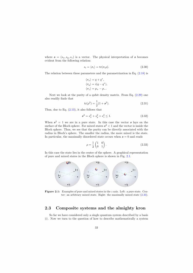
When s2 = 1 we are in a pure state. In this case the vector s lays on thesurface of the Bloch sphere. For mixed states s2 < 1 and the vector is inside theBloch sphere. Thus, we see that the purity can be directly associated with theradius in Bloch’s sphere. The smaller the radius, the more mixed is the state.In particular, the maximally disordered state occurs when s = 0 and reads

⇢ =1

2

✓1 00 1

◆. (2.33)

In this case the state lies in the center of the sphere. A graphical representationof pure and mixed states in the Bloch sphere is shown in Fig. 2.1.

Figure 2.1: Examples of pure and mixed states in the z axis. Left: a pure state. Cen-ter: an arbitrary mixed state. Right: the maximally mixed state (2.33).

2.3 Composite systems and the almighty kron

So far we have considered only a single quantum system described by a basis|ii. Now we turn to the question of how to describe mathematically a system

33