density functional theory › uploadeddocuments › admince › files › a… · timetable. d r....
TRANSCRIPT

QuickTime™ and aTIFF (LZW) decompressor
are needed to see this picture.
Density Functional Theory
Modulo: Funzionale Densità Chimica Computazionale
A.A. 2009-2010
Docente: Maurizio Casarin

QuickTime™ and aTIFF (LZW) decompressor
are needed to see this picture.
Chimica Computazionale
Academic Year 2009 - 2010 maurizio casarinSecond Semester
DFT allows to get information about theenergy, the structure and the molecularproperties of molecules at lower costs thattraditions approaches based on thewavefunction use.
Density functional theory (DFT) hasrevolutionized the quantun chemistrydevelopment of the last 20 years

QuickTime™ and aTIFF (LZW) decompressor
are needed to see this picture.
Chimica Computazionale
Academic Year 2009 - 2010 maurizio casarinSecond Semester
Quantum Methods
Wavefunctions Electron Density
Hartree-Fock DFT
TD-DFTMP2-CI
The HF equations have to be solved iteratively because VHF depends uponsolutions (the orbitals). In practice, one adopts the LCAO scheme, where theorbitals are expressed in terms of N basis functions, thus obtaining matricialequations depending upon N4 bielectron integrals.

QuickTime™ and aTIFF (LZW) decompressor
are needed to see this picture.
Chimica Computazionale
Academic Year 2009 - 2010 maurizio casarinSecond Semester
Correlation energy
Exchange correlation: Electrons with the same spin (ms) do not moveindependently as a consequence of the Pauliexclusion principle. = 0 if two electrons withthe same spin occupy the same point in space,independently of their charge. HF theory treatsexactly the exchange correlation generating anon local exchange correlation potential.
Coulomb correlation: Electrons cannot move independently as aconsequence of their Coulomb repulsion eventhough they are characterized by different spin(ms). HF theory completely neglects theCoulomb correlation thus generating, inprinciple, significant mistakes. Post HFtreatments are often necessary.

QuickTime™ and aTIFF (LZW) decompressor
are needed to see this picture.
Chimica Computazionale
Academic Year 2009 - 2010 maurizio casarinSecond Semester
x
y
z
dr1dr2
r1 r2
P r1,r2 dr1dr2
x1,x2 1 x1 2 x2
1 x1 1
rr1 1
2 x2 2
rr2 2
QuickTime™ and aTIFF (LZW) decompressor
are needed to see this picture.
Chimica Computazionale
Academic Year 2009 - 2010 maurizio casarinSecond Semester
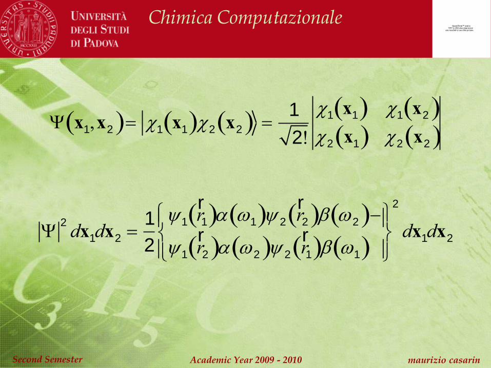
x1,x2 1 x1 2 x2 1
2!
1 x1 1 x2 2 x1 2 x2
2dx1dx2
1
2
1
rr1 1 2
rr2 2
1
rr2 2 2
rr1 1
2
dx1dx2

QuickTime™ and aTIFF (LZW) decompressor
are needed to see this picture.
Chimica Computazionale
Academic Year 2009 - 2010 maurizio casarinSecond Semester
x
y
z
dr1dr2
r1 r2
P r1,r2 dr1dr2
If the electrons have
not the same spin

QuickTime™ and aTIFF (LZW) decompressor
are needed to see this picture.
Chimica Computazionale
Academic Year 2009 - 2010 maurizio casarinSecond Semester
Prr1,
rr2 d
rr1d
rr2 d1d2
2
12 1
rr1
2
2
rr2
2
1
rr2
2
2
rr1
2
drr1d
rr2
if
P
rr1,
rr2 1
rr1
2
1
rr2
2
1 2
P
rr1,
rr1 1
rr1
2
1
rr1
2
0

QuickTime™ and aTIFF (LZW) decompressor
are needed to see this picture.
Chimica Computazionale
Academic Year 2009 - 2010 maurizio casarinSecond Semester
x
y
z
dr1dr2
r1 r2
P r1,r2 dr1dr2
If the electrons have
the same spin

QuickTime™ and aTIFF (LZW) decompressor
are needed to see this picture.
Chimica Computazionale
Academic Year 2009 - 2010 maurizio casarinSecond Semester
Prr1,
rr2 1
2
1
rr1
2
2
rr2
2
1
rr2
2
2
rr2
2
1
* rr1 2
rr1 2
* rr2 1
rr2
1
rr1 2
* rr1 2
rr2 1
* rr2
1 x1 1
rr1 1
2 x2 2
rr2 2
Prr1,
rr1 0

QuickTime™ and aTIFF (LZW) decompressor
are needed to see this picture.
Chimica Computazionale
Academic Year 2009 - 2010 maurizio casarinSecond Semester
Information provided by is redundant
QuickTime™ and a decompressor
are needed to see this picture.benzene
Number of terms in the determinantal form : N! = 1.4 1051
Number of Cartesian dimensions: 3N = 126
is a very complex object including more information than we need!
N = 42e-

QuickTime™ and aTIFF (LZW) decompressor
are needed to see this picture.
Chimica Computazionale
Academic Year 2009 - 2010 maurizio casarinSecond Semester
The use of electron density allows to limitthe redundant information
The electron density is a function of threecoordinates no matter of the electronnumber.

QuickTime™ and aTIFF (LZW) decompressor
are needed to see this picture.
Chimica Computazionale
Academic Year 2009 - 2010 maurizio casarinSecond Semester
• 1920s: Introduction of the Thomas-Fermi model.• 1964: Hohenberg-Kohn paper proving existence of exact DF.• 1965: Kohn-Sham scheme introduced.• 1970s and early 80s: LDA. DFT becomes useful.• 1985: Incorporation of DFT into molecular dynamics (Car-Parrinello)
(Now one of PRL’s top 10 cited papers).• 1988: Becke and LYP functionals. DFT useful for some chemistry.• 1998: Nobel prize awarded to Walter Kohn in chemistry for development
of DFT.
Timetable

QuickTime™ and aTIFF (LZW) decompressor
are needed to see this picture.
Chimica Computazionale
Academic Year 2009 - 2010 maurizio casarinSecond Semester
Quotation: “If I have seen further [than certain other men] it is by standing upon the shoulders of giants.”*
Isaac Newton (1642–1727), British physicist, mathematician. Letter to Robert Hooke, February 5, 1675.
*With reference to his dependency on Galileo’s and Kepler’s work in physics and astronomy.

QuickTime™ and aTIFF (LZW) decompressor
are needed to see this picture.
Chimica Computazionale
Academic Year 2009 - 2010 maurizio casarinSecond Semester
(a) Thomas, L. H. Proc. Cambridge Philos. Soc. 1927, 23, 542;(b) Fermi, E. Z. Phys. 1928, 48, 73;(c) Dirac, P. A. M. Cambridge Philos. Soc. 1930, 26, 376;(d) Wigner, E. P. Phys. Rev. 1934, 46, 1002.
QuickTime™ and a decompressor
are needed to see this picture.
Thomas, L. H.1903-1992
QuickTime™ and a decompressor
are needed to see this picture.
Fermi, E.1901-1954
QuickTime™ and a decompressor
are needed to see this picture.
Dirac, P.M.A.1902-1984
QuickTime™ and a decompressor
are needed to see this picture.
Wigner, E.1902-1995

QuickTime™ and aTIFF (LZW) decompressor
are needed to see this picture.
QuickTime™ and a decompressor
are needed to see this picture.
Hartree, D.R.1897-1958
QuickTime™ and a decompressor
are needed to see this picture.
Fock, D.R.1898-1974
(a) Hartree, D. R. Proc. Cambridge Phil. Soc. 1928, 24, 89; (b) ibidem 1928, 24, 111; (c) ibidem 1928, 24, 426; (d) Fock, V. Z. Physic 1930, 61, 126; (e) Slater, J. C. Phys. Rev. 1930, 35, 210.
QuickTime™ and aTIFF (LZW) decompressor
are needed to see this picture.
Slater J. C. 1900 -1976

QuickTime™ and aTIFF (LZW) decompressor
are needed to see this picture.
Chimica Computazionale
Academic Year 2009 - 2010 maurizio casarinSecond Semester
Definitions
Function: a prescription which maps one or more numbers toanother number:
y f x x2

QuickTime™ and aTIFF (LZW) decompressor
are needed to see this picture.
Chimica Computazionale
Academic Year 2009 - 2010 maurizio casarinSecond Semester
Definitions
Operator: a prescription which maps a function onto anotherfunction:
F 2
x2
Ff x 2 f x x2

QuickTime™ and aTIFF (LZW) decompressor
are needed to see this picture.
Chimica Computazionale
Academic Year 2009 - 2010 maurizio casarinSecond Semester
DefinitionsFunctional: A functional takes a function as input and gives
a number as output. An example is:
F[ f ] = f (x)dx–
F f x y
Here f(x) is a function and y is a number. An example is the
functional to integrate x from - to .
QuickTime™ and a decompressor
are needed to see this picture.
Vito Volterra1860 - 1940

QuickTime™ and aTIFF (LZW) decompressor
are needed to see this picture.
Chimica Computazionale
Academic Year 2009 - 2010 maurizio casarinSecond Semester
Francesco ed Edoardo Ruffini e Fabio Luzzatto (giuristi);Giorgio Levi Della Vida (orientalista);Gaetano De Sanctis (storico dell'antichità);Ernesto Buonaiuti (teologo);Vito Volterra (matematico);Bartolo Nigrisoli (chirurgo);Marco Carrara (antropologo);Lionello Venturi (storico dell'arte);Giorgio Errera (chimico);Piero Martinetti (studioso di filosofia).
In base a un regio decreto emanato il 28 agosto 1931 i docentidelle università italiane avrebbero dovuto giurare di esserefedeli non solo allo statuto albertino e alla monarchia, maanche al regime fascista.

QuickTime™ and aTIFF (LZW) decompressor
are needed to see this picture.
Chimica Computazionale
Academic Year 2009 - 2010 maurizio casarinSecond Semester
Nel 1938, con la promulgazione delle Leggi razziali, perdettero il posto iprofessori considerati di origine ebraica in base alla normativa razziale
QuickTime™ and a decompressor
are needed to see this picture.

QuickTime™ and aTIFF (LZW) decompressor
are needed to see this picture.
Chimica Computazionale
Academic Year 2009 - 2010 maurizio casarinSecond Semester
QuickTime™ and a decompressor
are needed to see this picture.
QuickTime™ and a decompressor
are needed to see this picture.

QuickTime™ and aTIFF (LZW) decompressor
are needed to see this picture.
Chimica Computazionale
Academic Year 2009 - 2010 maurizio casarinSecond Semester
ab-initio methods can be interpreted as afunctional of the wavefunction, with thefunctional form completely known!
E *
x1,L , xN H x1,L , xN dx1L dxN
*
x1,L , xN x1,L , xN dx1L dxN

QuickTime™ and aTIFF (LZW) decompressor
are needed to see this picture.
Chimica Computazionale
Academic Year 2009 - 2010 maurizio casarinSecond Semester
Electrons are uniformly distributedover the phase space in cells of 2h
3
Each cell may contain up to twoelectrons with opposite spins
Thomas–Fermi-Dirac Model
Electrons experience a potential fieldgenerated by the nuclear charge and bythe electron distribution itself.

QuickTime™ and aTIFF (LZW) decompressor
are needed to see this picture.
Chimica Computazionale
Academic Year 2009 - 2010 maurizio casarinSecond Semester
QuickTime™ and a decompressor
are needed to see this picture.
W
m
Let us consider a free electron gas

QuickTime™ and aTIFF (LZW) decompressor
are needed to see this picture.
Chimica Computazionale
Academic Year 2009 - 2010 maurizio casarinSecond Semester
Let us consider a free electron gas
N A
V 6.023 1023 atoms
mol 8.92 g
cm3
63.5 g
mol
8.47 1022 electrons
cm3
P 82.06 cm3atm
molK 293K
7.11 cm3
mol 3381atm
7.11 cm3
mol 6.023 1023 atomsmol
8.47 1022 electrons
cm3
N A
V 6.0231023 atoms
mol Z
at.weight
QuickTime™ and aTIFF (LZW) decompressor
are needed to see this picture.
Chimica Computazionale
Academic Year 2009 - 2010 maurizio casarinSecond Semester
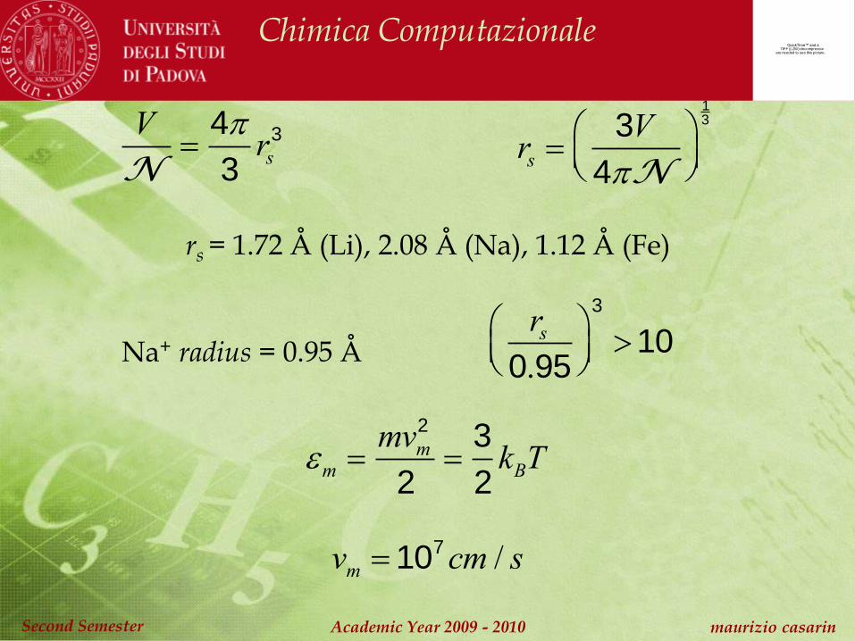
V
N
4
3rs
3
rs
3V
4N
13
rs = 1.72 Å (Li), 2.08 Å (Na), 1.12 Å (Fe)
Na+ radius = 0.95 Å
rs
0.95
3
10
m
mvm2
2
3
2kBT
vm 107cm / s

QuickTime™ and aTIFF (LZW) decompressor
are needed to see this picture.
Chimica Computazionale
Academic Year 2009 - 2010 maurizio casarinSecond Semester
QuickTime™ and a decompressor
are needed to see this picture.
m

QuickTime™ and aTIFF (LZW) decompressor
are needed to see this picture.
Chimica Computazionale
Academic Year 2009 - 2010 maurizio casarinSecond Semester
Main Assumption: independent electron approximation
V(r) = constant
H
2
2m2 V r
E
2
2m2 E
Aeik r
2
2mk2 E
E
2
2mk2
Let see what happens when QM is applied

QuickTime™ and aTIFF (LZW) decompressor
are needed to see this picture.
Chimica Computazionale
Academic Year 2009 - 2010 maurizio casarinSecond Semester
Aeik r
p i
r i
rAeik r k
De Broglie relation states that
p h
k k
2

QuickTime™ and aTIFF (LZW) decompressor
are needed to see this picture.
Chimica Computazionale
Academic Year 2009 - 2010 maurizio casarinSecond Semester
0 L 0
n
2
L
12
sinnx
L
En
2
2m
L
2
n2
QuickTime™ and a decompressor
are needed to see this picture.
Two kinds of boundary conditions

QuickTime™ and aTIFF (LZW) decompressor
are needed to see this picture.
Chimica Computazionale
Academic Year 2009 - 2010 maurizio casarinSecond Semester
x x L
x Aeikxx x L AeikxxeikxL eikxL 1
kxL 2m
m x L 1
2ei 2mxL
Em 2
2mk2
2
2m
2m
L
2
m 0,1,2,

QuickTime™ and aTIFF (LZW) decompressor
are needed to see this picture.
Chimica Computazionale
Academic Year 2009 - 2010 maurizio casarinSecond Semester
Moving to three dimensions
m x, y,z L32ei 2L mxxmyymzz
Em
2
2mk2
2
2m
2
L
2
mx2 my
2 mz2
mx ,my ,mz 0,1,2,
k
2
Lm

QuickTime™ and aTIFF (LZW) decompressor
are needed to see this picture.
Chimica Computazionale
Academic Year 2009 - 2010 maurizio casarinSecond Semester
m x, y,z L32ei 2L mxxmyymzz
Em
2
2m
2
L
2
mx2 my
2 mz2
k
2
Lm
k V 1
2eik r
Em
2
2mkx
2 ky2 kz
2

QuickTime™ and aTIFF (LZW) decompressor
are needed to see this picture.
Chimica Computazionale
Academic Year 2009 - 2010 maurizio casarinSecond Semester
Degeneracies of free electron levels
Typical possibilities Orbital
degeneracy
Total
degeneray
mx my mz m2
0 0 0 0 1 2
±1 0 0 1 6 12
±1 ±1 0 2 12 24
±1 ±1 ±1 3 8 16
±2 0 0 4 6 12
For large m values the degeneracies go up as m2
12

QuickTime™ and aTIFF (LZW) decompressor
are needed to see this picture.
Chimica Computazionale
Academic Year 2009 - 2010 maurizio casarinSecond Semester
mF mmax
Energy, temperature and velocity of electrons with mF
N 24
3
mF
3 24
3
V
2 3kF
3
EF
2
2mkF
2 2
2m
2
L
2
mF2
2
2m
3 2N
V
23
k
2
Lm
p i
r i
rAeik r k

QuickTime™ and aTIFF (LZW) decompressor
are needed to see this picture.
Chimica Computazionale
Academic Year 2009 - 2010 maurizio casarinSecond Semester
If we assume that the number of electrons per unit
volume is 0, then the Fermi momentum pF of a
uniform free electron gas is:
0
N
V
pF3
3 2h3
EF
pF2
2m
2
2m
3 2N
V
23
pF
3 2N
V
13

QuickTime™ and aTIFF (LZW) decompressor
are needed to see this picture.
Chimica Computazionale
Academic Year 2009 - 2010 maurizio casarinSecond Semester
Thomas and Fermi applied such a relation to aninhomogeneous situation as that of atoms, molecules andsolids. If the inhomogeneous electron density is denotedby , when the equation defining 0 is applied locallyat , it yields
r r
r
pF3 r
3 2 3
QuickTime™ and aTIFF (LZW) decompressor
are needed to see this picture.
Chimica Computazionale
Academic Year 2009 - 2010 maurizio casarinSecond Semester
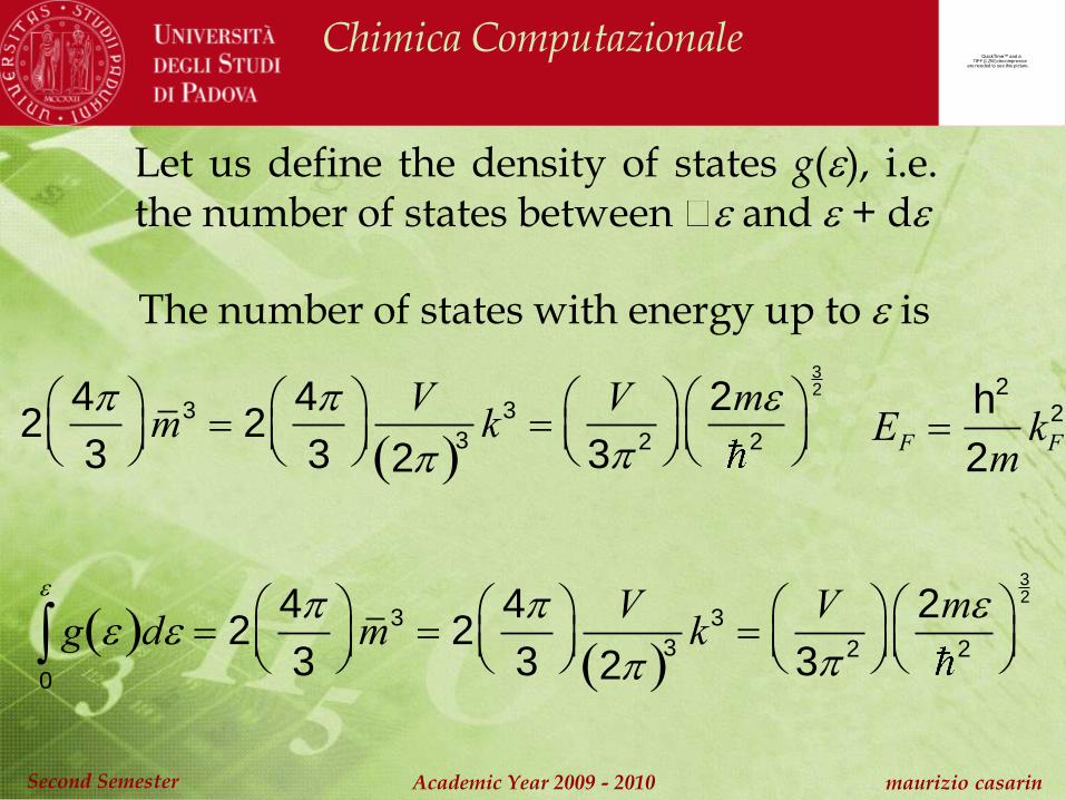
Let us define the density of states g(), i.e.the number of states between and + d
24
3
m3 2
4
3
V
2 3k3
V
3 2
2m
2
32
g d0
24
3
m3 2
4
3
V
2 3k3
V
3 2
2m
2
32
The number of states with energy up to is
EF
h2
2mkF
2

QuickTime™ and aTIFF (LZW) decompressor
are needed to see this picture.
Chimica Computazionale
Academic Year 2009 - 2010 maurizio casarinSecond Semester
g
3
2
V
3 2
2m
2
32
12 2
V
2
m
2
32
12 C
12
g d0
24
3
m3 2
4
3
V
2 3k3
V
3 2
2m
2
32

QuickTime™ and aTIFF (LZW) decompressor
are needed to see this picture.
Chimica Computazionale
Academic Year 2009 - 2010 maurizio casarinSecond Semester
T0 g d0
F
C 32d
0
F
2
5CF
52
F
pF2
2m
2
2m
3 2N
V
23
F
32
2
2m
32
3 2N
V
T0 2
5CF
52
2
52V
2
m
h2
32
C
1 24 4 34 4
h2
2m
32
3 2N
V
F
3
5NF
T0 = total kinetic energy
pF
3 2N
V
13

QuickTime™ and aTIFF (LZW) decompressor
are needed to see this picture.
Chimica Computazionale
Academic Year 2009 - 2010 maurizio casarinSecond Semester
T
rr
3h2
10m
3
8
23
Vrr
53
T0 0 2
52V
2
m
2
32
C
2
2m3 2
230
23
F
52
T0 0
3h2
10m
3
8
23
V0
53
T0
3
5NF
T0
2
5CF
52

QuickTime™ and aTIFF (LZW) decompressor
are needed to see this picture.
Chimica Computazionale
Academic Year 2009 - 2010 maurizio casarinSecond Semester
One can next write the classical energy equation for thefastest electrons as
pF2 r 2m
V r
2
2m
3 2
23 r
23 V r
r
pF3 r
3 2 3
The basic equation of the TF theory. It is aclassical expression, and consequently it can beapplied only in those cases for which – V > 0
h 3 2
13
rr
13 pF
rr

QuickTime™ and aTIFF (LZW) decompressor
are needed to see this picture.
Chimica Computazionale
Academic Year 2009 - 2010 maurizio casarinSecond Semester
TTF
rr CTF
53
rr d
rr
ETF r CTF 53 r dr Z
r r dr
1
2
r1 r2 r1—r2
dr1dr2
T
rr
3h2
10m
3
8
23
l 3rr
53
QuickTime™ and aTIFF (LZW) decompressor
are needed to see this picture.
Chimica Computazionale
Academic Year 2009 - 2010 maurizio casarinSecond Semester
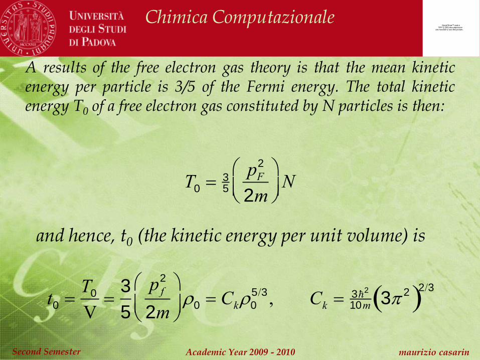
A results of the free electron gas theory is that the mean kineticenergy per particle is 3/5 of the Fermi energy. The total kineticenergy T0 of a free electron gas constituted by N particles is then:
T0
35
pF2
2m
N
and hence, t0 (the kinetic energy per unit volume) is
t0 T0
V
3
5
p f2
2m
0 Ck0
5/3 , Ck 3 2
10m 3 2 2/3

QuickTime™ and aTIFF (LZW) decompressor
are needed to see this picture.
Chimica Computazionale
Academic Year 2009 - 2010 maurizio casarinSecond Semester
t Ck r 5/3
E Ck r
5/3dr r VM r dr
e2
2
r r ' r r ' drdr '
The physical meaning of the last equation is that the electronicproperties of a system are determined as functionals of the electronicdensity by applying, locally, relations appropriate to a homogeneousfree electron gas. This approximation, known as local densityapproximation (LDA), is probably one of the most important conceptof the modern DFT!

QuickTime™ and aTIFF (LZW) decompressor
are needed to see this picture.
Chimica Computazionale
Academic Year 2009 - 2010 maurizio casarinSecond Semester
ETF TF
rr d
rr N 0
N N rr
rr d
rr
TF
ETF
rr
53CF
23
rr
rr
rr
Z
r
rr2
rr
rr2
drr2

QuickTime™ and aTIFF (LZW) decompressor
are needed to see this picture.
Chimica Computazionale
Academic Year 2009 - 2010 maurizio casarinSecond Semester
QuickTime™ and a decompressor
are needed to see this picture.

QuickTime™ and aTIFF (LZW) decompressor
are needed to see this picture.
Chimica Computazionale
Academic Year 2009 - 2010 maurizio casarinSecond Semester
v
X
HF vX
rr
;
rr 3
2 3
rr
1
3

QuickTime™ and aTIFF (LZW) decompressor
are needed to see this picture.
Chimica Computazionale
Academic Year 2009 - 2010 maurizio casarinSecond Semester
A non local operator is characterized by the general equation
r ' A dr A r ',r r ' r ' A r ',r r ' A r
r ' A r A r r ' r
QuickTime™ and aTIFF (LZW) decompressor
are needed to see this picture.
Chimica Computazionale
Academic Year 2009 - 2010 maurizio casarinSecond Semester
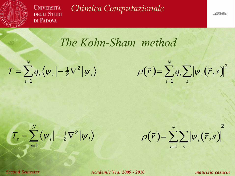
T qi i
i1
N
12
2 i
The Kohn-Sham method
r qi i r ,s
2
s
i1
N
Ts i
i1
N
12
2 i
r i r ,s
s
i1
N
2

QuickTime™ and aTIFF (LZW) decompressor
are needed to see this picture.
Chimica Computazionale
Academic Year 2009 - 2010 maurizio casarinSecond Semester
In ogni punto si associa alla densita alla densita (r) l’energia XC cheavrebbe un gas elettronico uniforme con la stessa densità. Ciò è ripetutoper ogni punto e i valori usati nelle formule
QuickTime™ and a decompressor
are needed to see this picture.

QuickTime™ and aTIFF (LZW) decompressor
are needed to see this picture.
Chimica Computazionale
Academic Year 2009 - 2010 maurizio casarinSecond Semester
QuickTime™ and a decompressor
are needed to see this picture.
Theodor
von Kàrmàn
George
de Hevesy
Michael
PolanyiLeo Szilard
Eugene
Wigner
John
von Neumann
Edward
Teller
The seven majar kings of science

QuickTime™ and aTIFF (LZW) decompressor
are needed to see this picture.
Chimica Computazionale
Academic Year 2009 - 2010 maurizio casarinSecond Semester
QuickTime™ and a decompressor
are needed to see this picture.
QuickTime™ and a decompressor
are needed to see this pict ure.
P. Hohenberg W. Kohn

QuickTime™ and aTIFF (LZW) decompressor
are needed to see this picture.
Chimica Computazionale
Academic Year 2009 - 2010 maurizio casarinSecond Semester
EHF
HF
öH HF
Hi
i1
N
1
2J
ijK
ij i, j1
N
H
i
i
*x 1
22 v x
i
x dx
Jij
ix
1 i
*x
1 1
r12
j
*x
2 jx
2 dx1dx
2
Kij
i
*x
1 jx
1 1
r12
ix
2 j
*x
2 dx1dx
2

QuickTime™ and aTIFF (LZW) decompressor
are needed to see this picture.
Chimica Computazionale
Academic Year 2009 - 2010 maurizio casarinSecond Semester
Minimization and orthonomalization conditions
öFix
ijj1
N
jx
öF 1
22 v ög

QuickTime™ and aTIFF (LZW) decompressor
are needed to see this picture.
Chimica Computazionale
Academic Year 2009 - 2010 maurizio casarinSecond Semester
• 1920s: Introduction of the Thomas-Fermi model.
• 1964: Hohenberg-Kohn paper proving existence of exact DF.
• 1965: Kohn-Sham scheme introduced.
• 1970s and early 80s: LDA. DFT becomes useful.
• 1985: Incorporation of DFT into molecular dynamics (Car-Parrinello)
(Now one of PRL’s top 10 cited papers).
• 1988: Becke and LYP functionals. DFT useful for some chemistry.
• 1998: Nobel prize awarded to Walter Kohn in chemistry for
development of DFT.
Background

QuickTime™ and aTIFF (LZW) decompressor
are needed to see this picture.
Chimica Computazionale
Academic Year 2009 - 2010 maurizio casarinSecond Semester
QuickTime™ and a decompressor
are needed to see this picture.

QuickTime™ and aTIFF (LZW) decompressor
are needed to see this picture.
Chimica Computazionale
Academic Year 2009 - 2010 maurizio casarinSecond Semester
The first HK theorem legitimates as basic variable.
The external potential is determined, within a
trivial additive constant, by the electron density.
Ev T Vem Vee r v r dr FHK
FHK T Vee
Vee J non classical terms

QuickTime™ and aTIFF (LZW) decompressor
are needed to see this picture.
Chimica Computazionale
Academic Year 2009 - 2010 maurizio casarinSecond Semester
The second HK theorem supplies the variational
principle for the ground state energy.
r dr N E0 Ev
Ev r dr N
0
The ground state energy and density correspond to the
minimum of some functional E subject to the constraint that
the density contains the correct number of electrons. The
Lagrange multiplier of this constraint is the electronic
chemical potential .

QuickTime™ and aTIFF (LZW) decompressor
are needed to see this picture.
Chimica Computazionale
Academic Year 2009 - 2010 maurizio casarinSecond Semester
In matematica e in fisica teorica, la derivata funzionale è una
generalizzazione della derivata direzionale. La differenza è
che la seconda differenzia nella direzione di un vettore,
mentre la prima differenzia nella direzione di una funzione.
Entrambe possono essere viste come estensioni dell'usuale
derivata.
F f r ,,,2, d3r
F
f
f
2 f
2

QuickTime™ and aTIFF (LZW) decompressor
are needed to see this picture.
Chimica Computazionale
Academic Year 2009 - 2010 maurizio casarinSecond Semester
J 1
2
r r ' r r '
d3r '
d3r
J
j
r ' r r ' d3r '
j
1
2
r r ' r r ' d3r '
2J 2
r ' r r ' d3r '
r ' r r '
1
r r '

QuickTime™ and aTIFF (LZW) decompressor
are needed to see this picture.
Chimica Computazionale
Academic Year 2009 - 2010 maurizio casarinSecond Semester
Ev r
v r FHK r
Ev T Vem Vee r v r dr FHK

QuickTime™ and aTIFF (LZW) decompressor
are needed to see this picture.
Chimica Computazionale
Academic Year 2009 - 2010 maurizio casarinSecond Semester
Despite the importance of the HK theorems, it is
noteworthy that the result they give is somehow
incomplete. Actually, the first HK theorem refers
only to the ground state energy and ground state
density. Furthermore, as far as the second HK
theorem is concerned, it is simply an existence
theorem and no information about how to get the
ground state energy functional is provided.
Nevertheless, the existence of an exact theory
justifies the research of new funtionals that, though
approximate version of the correct one, are more and
more accurate.

QuickTime™ and aTIFF (LZW) decompressor
are needed to see this picture.
Chimica Computazionale
Academic Year 2009 - 2010 maurizio casarinSecond Semester
• 1920s: Introduction of the Thomas-Fermi model.
• 1964: Hohenberg-Kohn paper proving existence of exact DF.
• 1965: Kohn-Sham scheme introduced.
• 1970s and early 80s: LDA. DFT becomes useful.
• 1985: Incorporation of DFT into molecular dynamics (Car-Parrinello)
(Now one of PRL’s top 10 cited papers).
• 1988: Becke and LYP functionals. DFT useful for some chemistry.
• 1998: Nobel prize awarded to Walter Kohn in chemistry for
development of DFT.
Background

QuickTime™ and aTIFF (LZW) decompressor
are needed to see this picture.
Chimica Computazionale
Academic Year 2009 - 2010 maurizio casarinSecond Semester
The Kohn-Sham method.
The massive usage of DFT is tightly bound to its use
in orbitalic theories. This is not very surprising
because of the role played by these theories, in
particular the HF one, in quantum chemistry. Thus,
the major DFT developments have implied either the
improvement of existing orbitalic theories, for
instance the X method [Slater, 1951a-b], or the
proposal of new approaches [Kohn & Sham, 1965].
QuickTime™ and aTIFF (LZW) decompressor
are needed to see this picture.
Chimica Computazionale
Academic Year 2009 - 2010 maurizio casarinSecond Semester
QuickTime™ and a decompressor
are needed to see this picture.

QuickTime™ and aTIFF (LZW) decompressor
are needed to see this picture.
Chimica Computazionale
Academic Year 2009 - 2010 maurizio casarinSecond Semester
Interacting electrons + real potential
Non-interacting fictitious particles + effective potential

QuickTime™ and aTIFF (LZW) decompressor
are needed to see this picture.
Chimica Computazionale
Academic Year 2009 - 2010 maurizio casarinSecond Semester
H s 1
2i
2 i
N
vs ri i
N
s
1
N !det 1 2 N
hs i 1
22 vs r i i i
Ts s 1
2i
2 i
N
s i 12
2 i
i
N

QuickTime™ and aTIFF (LZW) decompressor
are needed to see this picture.
Chimica Computazionale
Academic Year 2009 - 2010 maurizio casarinSecond Semester
F Ts J Exc J 1
21r12 r1 r2 dr1dr2
Exc T Ts Vee J
veff r Ts r
veff r v r J r
Exc r
v r r ' r r '
dr ' vxc r
Ev r
v r FHK r
vxc r Exc r

QuickTime™ and aTIFF (LZW) decompressor
are needed to see this picture.
Chimica Computazionale
Academic Year 2009 - 2010 maurizio casarinSecond Semester
With reference to the single Euler - Lagrange equation, the
introduction of N orbitals allows us to treat exactly Ts, the
dominant part of the true kinetic energy T[]. The cost we have
to pay is the needed of N equations rather than one expressed
in terms of the total electron density. The KS equations have
the same form of the Hartree equations unless the presence of
a more general local potential, . The computational effort
for their solution is comparable to that required for the Hartree
equations and definitely smaller than that pertinent to the HF
ones. HF equations are characterized by a one-electron
Hamiltonian including a non local potential and for this reason
they cannot be considered a special case of the KS equations.
veff r

QuickTime™ and aTIFF (LZW) decompressor
are needed to see this picture.
Chimica Computazionale
Academic Year 2009 - 2010 maurizio casarinSecond Semester
Relative magnitudes of contributions to
total valence energy (in eV) of the Mn atom

QuickTime™ and aTIFF (LZW) decompressor
are needed to see this picture.
Chimica Computazionale
Academic Year 2009 - 2010 maurizio casarinSecond Semester
The exchange-correlation potential
While DFT in principle gives a good description of ground
state properties, practical applications of DFT are based on
approximations for the so-called exchange-correlation
potential. The exchange-correlation potential describes the
effects of the Pauli principle and the Coulomb potential beyond
a pure electrostatic interaction of the electrons.
Possessing the exact exchange-correlation potential means
that we solved the many-body problem exactly.
A common approximation is the so-called local density
approximation (LDA) which locally substitutes the exchange-
correlation energy density of an inhomogeneous system by
that of an electron gas evaluated at the local density.

QuickTime™ and aTIFF (LZW) decompressor
are needed to see this picture.
Chimica Computazionale
Academic Year 2009 - 2010 maurizio casarinSecond Semester
The Local Density Approximation (LDA)The LDA approximation assumes that the density is slowlyvarying and the inhomogeneous density of a solid ormolecule can be calculated using the homogeneouselectron gas functional.While many ground state properties (lattice constants, bulk
moduli, etc.) are well described in the LDA, the dielectric
constant is overestimated by 10-40% in LDA compared to
experiment. This overestimation stems from the neglect of a
polarization-dependent exchange correlation field in LDA
compared to DFT.
The method can be improved by including the gradient of
the density into the functional. The generalized gradient
approximation GGA is an example of this type of approach.

QuickTime™ and aTIFF (LZW) decompressor
are needed to see this picture.
Chimica Computazionale
Academic Year 2009 - 2010 maurizio casarinSecond Semester
The Slater exchange functional
The predecessor to modern DFT is Slater’s X method.
This method was formulated in 1951 as an approximate
solution to the Hartree-Fock equations. In this method the
HF exchange was approximated by:
The exchange energy EX is a fairly simple function of the
electron density .
The adjustable parameter was empirically determined
for each atom in the periodic table. Typically is between
0.7 and 0.8. For a free electron gas = 2/3.
EX[] = – 94 3
4
1/3
4/3(r)dr0

QuickTime™ and aTIFF (LZW) decompressor
are needed to see this picture.
Chimica Computazionale
Academic Year 2009 - 2010 maurizio casarinSecond Semester
The VWN Correlation Functional
In ab initio calculations of the Hartree-Fock type electron
correlation is also not included. However, it can be included
by inclusion of configuration interaction (CI). In DFT
calculations the correlation functional plays this role. The
Vosko-Wilk-Nusair correlation function is often added to the
Slater exchange function to make a combination exchange-
correlation functional.
Exc = Ex + Ec
The nomenclature here is not standardized and the
correlation functionals themselves are very complicated
functions. The correlation functionals can be seen on the
MOLPRO website
http://www.molpro.net/molpro2002.3/doc/manual/node146.html.
QuickTime™ and aTIFF (LZW) decompressor
are needed to see this picture.
Chimica Computazionale
Academic Year 2009 - 2010 maurizio casarinSecond Semester
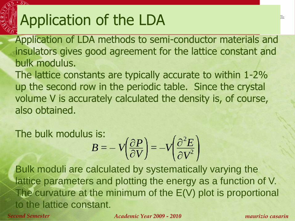
Application of the LDAApplication of LDA methods to semi-conductor materials and insulators gives good agreement for the lattice constant and bulk modulus.The lattice constants are typically accurate to within 1-2%up the second row in the periodic table. Since the crystalvolume V is accurately calculated the density is, of course,also obtained.
The bulk modulus is:
Bulk moduli are calculated by systematically varying the
lattice parameters and plotting the energy as a function of V.
The curvature at the minimum of the E(V) plot is proportional
to the lattice constant.
B = – V PV
= –V
2E
V2

QuickTime™ and aTIFF (LZW) decompressor
are needed to see this picture.
Chimica Computazionale
Academic Year 2009 - 2010 maurizio casarinSecond Semester
Generalized gradient approximation (GGA). Take density gradient into account. Useful for molecules.
Spin density functional theory. Two independent variables:density and magnetization.
Exact exchange density functional theory. Calculate exchange exactly and correlation approximately using DFT.
Generalized density functional theory. Modify K-S energy partitioning to obtain a non-local hamiltonian.
Extensions of the LDA approach
m(r) = – 0 –

QuickTime™ and aTIFF (LZW) decompressor
are needed to see this picture.
Chimica Computazionale
Academic Year 2009 - 2010 maurizio casarinSecond Semester
The GGA approach takes into account variations in thedensity by including the gradient of the density in thefunctional. One commonly used GGA functional is that ofBecke.
This functional has only one adjustable parameter, . Thevalue of = 0.0042 was determined based on the best fitto the energies of six noble gas atoms using the sum of theLDA and GGA exchange terms.
The GGA option in DMol3 is that of Perdew and Wang.
Generalized Gradient Approach (GGA)
Vxc
B= – 1/3 x2
1 + 6x sinh– 1
x, x =
4/3

QuickTime™ and aTIFF (LZW) decompressor
are needed to see this picture.
Chimica Computazionale
Academic Year 2009 - 2010 maurizio casarinSecond Semester
As was discussed above for the Slater exchange functional(no gradient), the VWN correlation functional provides asignificant improvement in the calculation of the energiesand properties such as bulk modulus, vibrationalfrequencies etc. In a similar manner the Becke exchangefunctional (including a gradient correlation) and the Lee-Yang-Parr functional are used together. The Lee-Yang-Parror LYP correlation functional is quite complicated. It can beviewed on the MOLPRO website.
Thus, two of the most commonly used functionals are:S-VWN Slater exchange - VWN correlation (no gradients)B-LYP Becke exchange - LYP correlation (gradients)
Lee-Yang-Parr Correlation Functional

DFT Lecture, The 4th Summer School for Integrated Computational Materials Education
Integrated Computational Materials
Engineering Education
Lecture on Density Functional Theory
An Introduction
Mark Asta
Department of Materials Science and Engineering
University of California, Berkeley
Berkeley, CA 94720

DFT Lecture, The 4th Summer School for Integrated Computational Materials Education
Acknowledgements
• Portions of these lectures are based on material put together
by Daryl Chrzan (UC Berkeley) and Jeff Grossman (MIT) as
part of a TMS short course that the three of us taught at the
2010 annual meeting.
• The Division of Materials Research at the National Science
Foundation is acknowledged for financial support in the
development of the lecture and module

DFT Lecture, The 4th Summer School for Integrated Computational Materials Education
Use of DFT in Materials Research
K. Thornton, S. Nola, R. E. Garcia, MA and G. B. Olson, “Computational Materials Science and
Engineering Education: A Survey of Trends and Needs,” JOM (2009)

DFT Lecture, The 4th Summer School for Integrated Computational Materials Education
The Role of Electronic Structure Methods in ICME
• A wide variety of relevant properties can be calculated from
knowledge of atomic numbers alone
– Elastic constants
– Finite-temperature thermodynamic and transport properties
– Energies of point, line and planar defects
• For many classes of systems accuracy is quite high
– Can be used to obtain “missing” properties in materials design when
experimental data is lacking, hard to obtain, or “controversial”
– Can be used to discover new stable compounds with target properties
• The starting point for “hierarchical multiscale” modeling
– Enables development of interatomic potentials for larger-scale classical
modeling
DFT Lecture, The 4th Summer School for Integrated Computational Materials Education
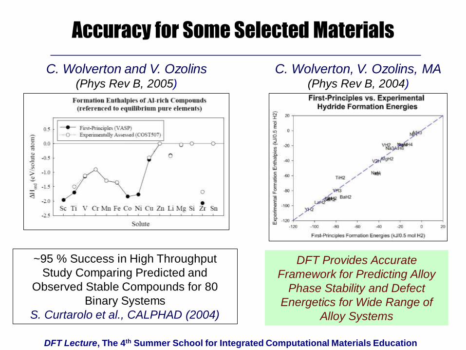
Accuracy for Some Selected Materials
DFT Provides Accurate
Framework for Predicting Alloy
Phase Stability and Defect
Energetics for Wide Range of
Alloy Systems
C. Wolverton and V. Ozolins(Phys Rev B, 2005)
C. Wolverton, V. Ozolins, MA(Phys Rev B, 2004)
~95 % Success in High Throughput
Study Comparing Predicted and
Observed Stable Compounds for 80
Binary Systems
S. Curtarolo et al., CALPHAD (2004)

DFT Lecture, The 4th Summer School for Integrated Computational Materials Education
1st-Principles Modeling of Alloy Phase Stability
Mixing Energies of BCC Fe-CuJ. Z. Liu, A. van de Walle, G. Ghosh and
MA (2005)
Solvus Boundaries in Al-TiJ. Z. Liu, G. Ghosh, A. van de Walle and
MA (2006)
Predictions for Both Stable and Metastable Phases
DFT Lecture, The 4th Summer School for Integrated Computational Materials Education
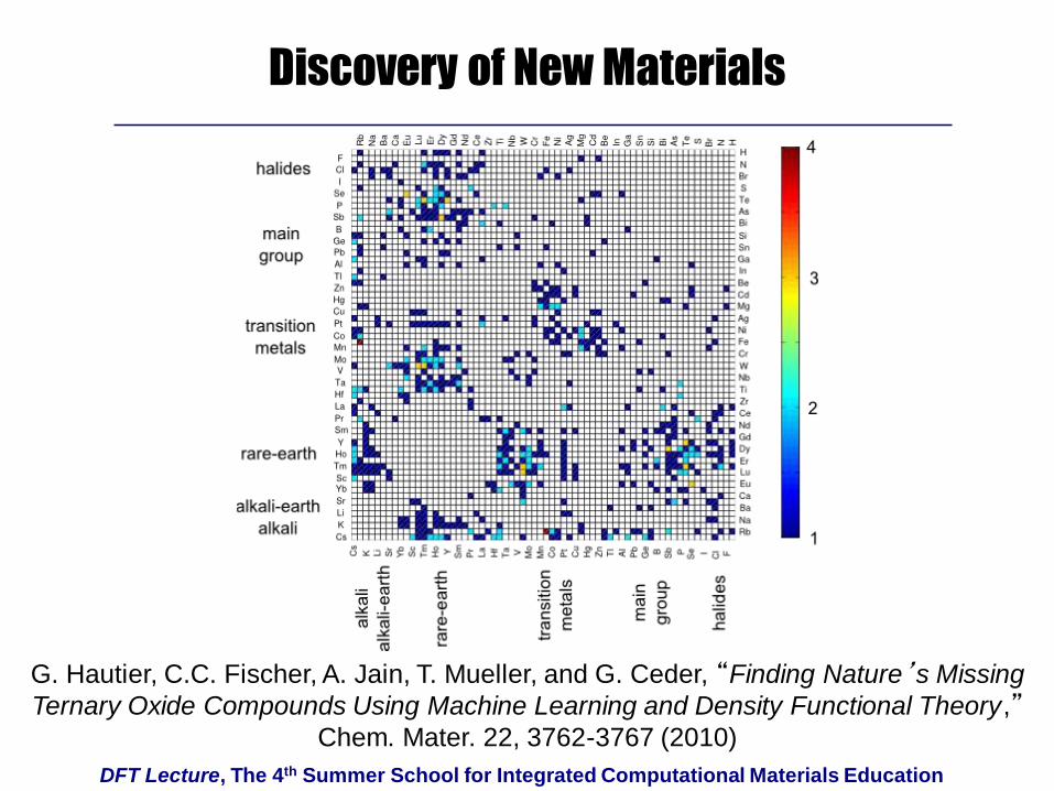
Discovery of New Materials
G. Hautier, C.C. Fischer, A. Jain, T. Mueller, and G. Ceder, “Finding Nature’s Missing
Ternary Oxide Compounds Using Machine Learning and Density Functional Theory,”Chem. Mater. 22, 3762-3767 (2010)

DFT Lecture, The 4th Summer School for Integrated Computational Materials Education
Materials Data for Discovery & Design
A. Jain, S.P. Ong, G. Hautier, W. Chen, W.D. Richards, S.
Dacek, S. Cholia, D. Gunter, D. Skinner, G. Ceder, K.A.
Persson, Applied Physics Letters Materials, 2013, 1(1), 011002.
https://www.materialsproject.org/

DFT Lecture, The 4th Summer School for Integrated Computational Materials Education
Outline
• Formalism
– Hydrogen Atom
– Density Functional Theory
• Exchange-Correlation Potentials
• Pseudopotentials and Related Approaches
• Some Commercial and Open Source Codes
• Practical Issues
– Implementation
• Periodic boundary conditions
• k-Points
• Plane-wave basis sets
– Parameters controlling numerical precision
• Example Exercise

DFT Lecture, The 4th Summer School for Integrated Computational Materials Education
IntroductionThe Hydrogen Atom
Proton with mass M1, coordinate R1
Electron with mass m1, coordinate r1
r = r1 - r2, R =M1R1 + m2r2
M1 + m2
, m =M1m2
M1 + m2
, M = M1 + m2
Y(R,r) =ycm (R)yr(r)
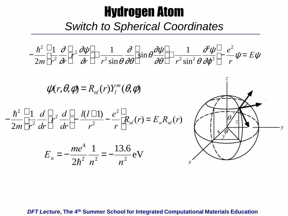
DFT Lecture, The 4th Summer School for Integrated Computational Materials Education
Hydrogen AtomSwitch to Spherical Coordinates
-2
2m
1
r2
¶rr2 ¶y
¶r
æ
è ç
ö
ø ÷ +
1
r2 sinq
¶qsinq
¶y
¶q
æ
è ç
ö
ø ÷ +
1
r2 sin2 q
¶2y
¶j2
æ
è ç
ö
ø ÷ -e2
ry = Ey
y(r,q,f) = Rnl (r)Ylm (q,f)
-2
2m
1
r2
d
drr2 d
dr
æ
è ç
ö
ø ÷ -l(l +1)
r2-e2
r
æ
è ç
ö
ø ÷ Rnl (r) = EnRnl (r)
En = -me4
2 2
1
n2= -
13.6
n2eV
q
f

DFT Lecture, The 4th Summer School for Integrated Computational Materials Education
Hydrogen AtomWavefunctions
n = 1, 2, 3, …
l = 0 (s), 1(p), 2(d), …, n-1
Probability densities through the xz-plane for the
electron at different quantum numbers (l, across
top; n, down side; m = 0)
http://en.wikipedia.org/wiki/Hydrogen_atom
http://galileo.phys.virginia.edu/classes/751.mf1i.fall02/HydrogenAtom.htm

DFT Lecture, The 4th Summer School for Integrated Computational Materials Education
The Many-Electron Problem
• collection of
– N ions
– n electrons
• total energy
computed as a
function of ion
positions
– must employ
quantum mechanics
electrons
ions

DFT Lecture, The 4th Summer School for Integrated Computational Materials Education
Born-Oppenheimer Approximation
• Mass of nuclei exceeds that of the electrons by a factor of
1000 or more
– we can neglect the kinetic energy of the nuclei
– treat the ion-ion interaction classically
– significantly simplifies the Hamiltonian for the electrons
• Consider Hamiltonian for n electrons in potential of N
nuclei with atomic numbers Zi
external potential
ºVext rj( )

DFT Lecture, The 4th Summer School for Integrated Computational Materials Education
Density Functional TheoryHohenberg and Kohn (1964), Kohn and Sham (1965)
• For each external potential there is a unique ground-
state electron density
• Energy can be obtained by minimizing of a density
functional with respect to density of electrons n(r)
Egroundstate=min{Etot[n(r)]}
Etot n r( )[ ] =T n r( )[ ] +Eint n r( )[ ] + drVext r( )ò n r( ) +Eion-ion
Kinetic Energy Electron-Electron
Interactions
Electron-Ion
Interactions

DFT Lecture, The 4th Summer School for Integrated Computational Materials Education
Kohn-Sham Approach
n(r) = -e fi(r)2
i=1
n
å
Many-Body Electron-Electron Interactions Lumped into Exc[n(r)]
“Exchange-Correlation Energy”

DFT Lecture, The 4th Summer School for Integrated Computational Materials Education
Kohn-Sham Equations
Vxc (r) ºdExc[n(r)]
dn(r)

DFT Lecture, The 4th Summer School for Integrated Computational Materials Education
Local Density Approximation(e.g., J. P. Perdew and A. Zunger, Phys. Rev. B 23, 5048 (1981))
Exc[n(r)] = exchomò (n(r))n(r)d3r

DFT Lecture, The 4th Summer School for Integrated Computational Materials Education
Generalized Gradient ApproximationJ. P. Perdew, K. Burke and M. Ernzerhof, Phys. Rev. Lett. 77 (1996)
ExcGGA[n(r)] = ex
homò (n(r))n(r)Fxc(rs,z, s)d3r
n = 3/ 4p rs3 = kF
3 / 3p 2
z = (n -n¯) / n
s =|Ñn | /2kFn

DFT Lecture, The 4th Summer School for Integrated Computational Materials Education
A Note on Accuracy and Ongoing Research
• LDA leads to “overbinding”− Lattice constants commonly 1-3 % too small, elastic constants 10-
15 % too stiff, cohesive energies 5-20 % too large
• BUT, errors are largely systematic
− Energy differences tend to be more accurate
• GGA corrects for overbinding
− Sometimes “overcorrects”
• “Beyond DFT” Approaches
− For “highly correlated” systems LDA & GGA perform much worse
and corrections required (DFT+U, Hybrid Hartree-Fock/DFT, …)
− Non-bonded interactions, e.g., van der Waals interactions in
graphite, require additional terms or functionals (e.g., vdW-DF)

DFT Lecture, The 4th Summer School for Integrated Computational Materials Education
Pseudopotentials
• Potential due to ions is
singular at ion core
• Eigenfunctions oscillate
rapidly near singularity
• Eigenfunction in bonding
region is smooth

DFT Lecture, The 4th Summer School for Integrated Computational Materials Education
Pseudopotentials
• For plane-wave basis sets, rapid oscillations
require large number of basis functions
– expensive
– unnecessary
• these oscillations don't alter bonding
properties
• Replace potential with nonsingular potential
– preserve bonding tails of eigenfunction
– preserve distribution of charge between core
and tail regions
– reduces number of plane waves required for
accurate expansion of wavefunction
• Transferable
– developed from properties of isolated atoms
– applied in other situations
f
fpseudo

DFT Lecture, The 4th Summer School for Integrated Computational Materials Education
Summary of Approaches
• Pseudopotentials
– Core electrons removed from problem and enter only in their
effect of the pseudopotential felt by the valence electrons
– Kohn-Sham equations solved for valence electrons only
• “Augment” Plane Waves with atomic-like orbitals
– An efficient basis set that allows all electrons to be treated in the
calculations
– Basis for “all-electron” codes
• Projector-Augmented-Wave method
– Combines features of both methods
– Generally accepted as the basis for the most accurate approach
for calculations requiring consideration of valence electrons only

DFT Lecture, The 4th Summer School for Integrated Computational Materials Education
Some of the Widely Used Codes
• VASP (http://cms.mpi.univie.ac.at/vasp/)
– Commercial, Plane-Wave Basis, Pseudopotentials and PAW
• PWSCF (http://www.quantum-espresso.org/)
– Free (and available to run on nanohub), Plane-Wave Basis,
Pseudopotentials and PAW
• CASTEP (http://ccpforge.cse.rl.ac.uk/gf/project/castep/)
– Free in UK, licensed by Accelrys elsewhere, Plane-Wave Basis,
Pseudopotentials
• ABINIT (http://www.abinit.org/)
– Free (and available to run on nanohub), plane-wave basis,
pseudopotentials and PAW
• WIEN2K (http://www.wien2k.at/)
– Commercial (modest license fee), all-electron augmented wave method

DFT Lecture, The 4th Summer School for Integrated Computational Materials Education
Outline
• Formalism
– Hydrogen Atom
– Density Functional Theory
• Exchange-Correlation Potentials
• Pseudopotentials and Related Approaches
• Some Commercial and Open Source Codes
• Practical Issues
– Implementation
• Periodic boundary conditions
• k-Points
• Plane-wave basis sets
– Parameters controlling numerical precision
• Example Exercise

DFT Lecture, The 4th Summer School for Integrated Computational Materials Education
Total Energy in Density Functional Theory
n(r) = -e fi(r)2
i=1
n
åElectron Density
Electron Wavefunctions fi(r)
Exchange-Correlation Energy Exc[n(r)]
Form depends on whether you use LDA or GGA
Potential Electrons Feel from Nuclei Vext (r)

DFT Lecture, The 4th Summer School for Integrated Computational Materials Education
Kohn-Sham EquationsSchrödinger Equation for Electron Wavefunctions
-2
2meÑi
2 +Vext (r)+n(r ')
r - r 'ò d3r '+Vxc (r)
é
ëêê
ù
ûúúfi(r) = eifi (r)
Vxc (r) ºdExc[n(r)]
dn(r)
Note: fi depends on n(r) which depends on fi
Solution of Kohn-Sham equations must be done iteratively
n(r) = -e fi(r)2
i=1
n
å
Exchange-Correlation Potential
Electron Density

DFT Lecture, The 4th Summer School for Integrated Computational Materials Education
Self-Consistent Solution to DFT Equations
Input Positions of Atoms for a Given
Unit Cell and Lattice Constant
guess charge density
compute effective
potential
compute Kohn-Sham
orbitals and density
compare output and
input charge densities
Energy for Given
Lattice Constant
different
same
1. Set up atom positions
2. Make initial guess of “input” charge density
(often overlapping atomic charge densities)
3. Solve Kohn-Sham equations with this input
charge density
4. Compute “output” charge density from
resulting wavefunctions
5. If energy from input and output densities
differ by amount greater than a chosen
threshold, mix output and input density and
go to step 2
6. Quit when energy from input and output
densities agree to within prescribed
tolerance (e.g., 10-5 eV)
Note: In your exercise, positions of atoms are dictated by symmetry. If this is not the
case another loop must be added to minimize energy with respect to atomic positions.

DFT Lecture, The 4th Summer School for Integrated Computational Materials Education
Implementation of DFT for a Single Crystal
aa
a
Unit Cell Vectors
a1 = a (-1/2, 1/2 , 0)
a2 = a (-1/2, 0, 1/2)
a3 = a (0, 1/2, 1/2)
Example: Diamond Cubic Structure of Si
Crystal Structure Defined by Unit Cell Vectors and Positions of
Basis Atoms
Basis Atom Positions
0 0 0
¼ ¼ ¼
All atoms in the crystal can be obtained by adding integer
multiples of unit cell vectors to basis atom positions
DFT Lecture, The 4th Summer School for Integrated Computational Materials Education
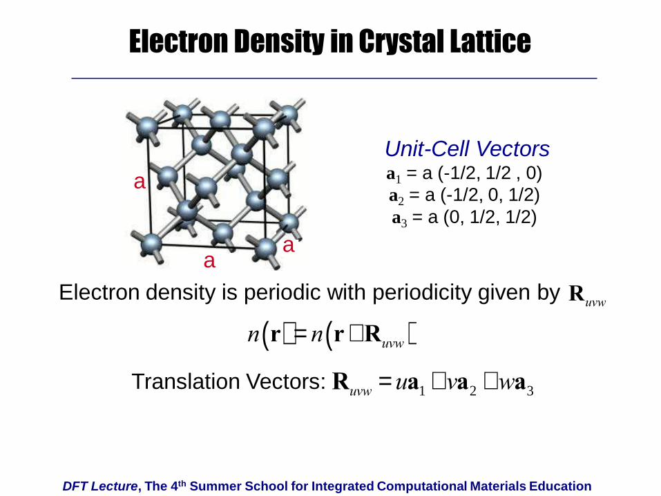
Electron Density in Crystal Lattice
n r( ) = n r+Ruvw( )
aa
a
Unit-Cell Vectorsa1 = a (-1/2, 1/2 , 0)
a2 = a (-1/2, 0, 1/2)
a3 = a (0, 1/2, 1/2)
Electron density is periodic with periodicity given by Ruvw
Ruvw = ua1 +va2 +wa3Translation Vectors:

DFT Lecture, The 4th Summer School for Integrated Computational Materials Education
Electronic BandstructureExample for Si
http://de.wikipedia.org/wiki/Datei:Band_structure_Si_schematic.svg
http://en.wikipedia.org/wiki/Brillouin_zone
Electronic wavefunctions in a crystal can be indexed by
point in reciprocal space (k) and a band index (b)
Brillouin Zone Bandstructure

DFT Lecture, The 4th Summer School for Integrated Computational Materials Education
Why?Wavefunctions in a Crystal Obey Bloch’s Theorem
fkbr( ) = exp ik ×r( ) uk
br( )
For a given band b
Where is periodic in real space: ukbr( ) = uk
br+Ruvw( )uk
br( )
Ruvw = ua1 +va2 +wa3Translation Vectors:

DFT Lecture, The 4th Summer School for Integrated Computational Materials Education
Representation of Electron Density
fkbr( ) = exp ik ×r( ) uk
br( )
n(r) = -e fkb r( )
WBZò
2
f (ekb -eF )
d3k
WBZb
å
In practice the integral over the Brillouin zone is replaced
with a sum over a finite number of k-points (Nkpt)
One parameter that needs to be checked for numerical
convergence is number of k-points
n(r) » -e w j fk jb r( )
2
j=1
Nkpt
å f (ek jb -eF )
b
å
Integral over k-points in first Brillouin zone
f(e-eF) is Fermi-Dirac distribution function with Fermi energy eF
n(r) = -e fi(r)2
i=1
Ne
å

DFT Lecture, The 4th Summer School for Integrated Computational Materials Education
Representation of WavefunctionsFourier-Expansion as Series of Plane Waves
ukbr( ) = uk
bGlmn( )exp iGlmn ×r( )
lmn
å
fkbr( ) = exp ik ×r( ) uk
br( )For a given band:
Recall that is periodic in real space: ukbr( ) = uk
br+Ruvw( )uk
br( )
can be written as a Fourier Series:ukbr( )
Glmn = la1
* +ma2
* +na3
*
where the are primitive reciprocal lattice vectorsa i*
a1
* ×a1 = 2p a1
* ×a2 = 0 a1
* ×a3 = 0
a2
* ×a1 = 0 a2
* ×a2 = 2p a2
* ×a3 = 0
a3
* ×a1 = 0 a3
* ×a2 = 0 a3
* ×a3 = 2p

DFT Lecture, The 4th Summer School for Integrated Computational Materials Education
Recall Properties of Fourier Series
http://mathworld.wolfram.com/FourierSeriesTriangleWave.html
Black line = (exact) triangular wave
Colored lines = Fourier series
truncated at different orders
General Form of Fourier Series:
For Triangular Wave:
Typically we expect the accuracy of a truncated Fourier series to
improve as we increase the number of terms

DFT Lecture, The 4th Summer School for Integrated Computational Materials Education
Representation of WavefunctionsPlane-Wave Basis Set
fkbr( ) = exp ik ×r( ) uk
br( )
Another parameter that needs to be checked for convergence is
the “plane-wave cutoff energy” Ecut
In practice the Fourier series is truncated to include all G for which:
2
2mG+ k( )
2< Ecut
For a given band
fkbr( ) = uk
bG( )exp i G+k( ) ×réë ùû
G
å
Use Fourier Expansion

DFT Lecture, The 4th Summer School for Integrated Computational Materials Education
Examples of Convergence Checks
Effect of Ecut Effect of Number of k Points
http://www.fhi-berlin.mpg.de/th/Meetings/FHImd2001/pehlke1.pdf

DFT Lecture, The 4th Summer School for Integrated Computational Materials Education
Outline
• Formalism
– Hydrogen Atom
– Density Functional Theory
• Exchange-Correlation Potentials
• Pseudopotentials and Related Approaches
• Some Commercial and Open Source Codes
• Practical Issues
– Implementation
• Periodic boundary conditions
• k-Points
• Plane-wave basis sets
– Parameters controlling numerical precision
• Example Exercise

DFT Lecture, The 4th Summer School for Integrated Computational Materials Education
Your Exercise: Part 1
• Calculate equation of state of diamond cubic Si using Quantum
Espresso on Nanohub (http://nanohub.org/)
• You will compare accuracy of LDA and GGA
• You will check numerical convergence with respect to number
of k-points and plane-wave cutoff
• You will make use of the following unit cell for diamond-cubic
structure
aa
a
Lattice Vectors
a1 = a (-1/2, 1/2 , 0)
a2 = a (-1/2, 0, 1/2)
a3 = a (0, 1/2, 1/2)
Basis Atom Positions
0 0 0
¼ ¼ ¼
DFT Lecture, The 4th Summer School for Integrated Computational Materials Education
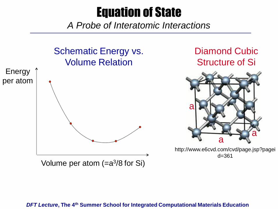
Equation of StateA Probe of Interatomic Interactions
aa
a
Energy
per atom
Volume per atom (=a3/8 for Si)
Schematic Energy vs.
Volume Relation
Diamond Cubic
Structure of Si
http://www.e6cvd.com/cvd/page.jsp?pagei
d=361

DFT Lecture, The 4th Summer School for Integrated Computational Materials Education
Equation of StateWhat Properties Can we Learn from It?
Pressure versus Volume Relation
Equilibrium Volume (or Lattice Constant)
Bulk Modulus
P = -¶E
¶V
Given E(V) one can compute P(V) by taking derivative
B = -V¶P
¶V=V
¶2E
¶V 2
Volume corresponding to zero pressure = Volume where slope of E(V) is zero
≈ Volume measured experimentally at P = 1 atm
B related to curvature of E(V) Function
Recall 1st Law of Thermo: dE = T dS - P dV and consider T = 0 K

DFT Lecture, The 4th Summer School for Integrated Computational Materials Education
Your Exercise: Part 2Non-hydrostatic Stress and Strain
Stress-Strain Relations in Linear Elasticity
s ij = Cijkleklk,l
å
Consider Single Strain e33=e
s = C11es22 = C12e
Stress-Strain Relations in Linear Elasticity
Stress Strain
Cijkl Single-Crystal Elastic Constants
Voigt Notation (for Cubic Crystal)C3333=C2222=C1111=C11
C2233=C1133=C1122=C2211=C3311=C3322=C12

Lecture 8:
Introduction to Density
Functional Theory
Marie Curie Tutorial Series: Modeling Biomolecules
December 6-11, 2004
Mark Tuckerman
Dept. of Chemistry
and Courant Institute of Mathematical Science
100 Washington Square East
New York University, New York, NY 10003

Background
• 1920s: Introduction of the Thomas-Fermi model.
• 1964: Hohenberg-Kohn paper proving existence of exact DF.
• 1965: Kohn-Sham scheme introduced.
• 1970s and early 80s: LDA. DFT becomes useful.
• 1985: Incorporation of DFT into molecular dynamics (Car-Parrinello)
(Now one of PRL’s top 10 cited papers).
• 1988: Becke and LYP functionals. DFT useful for some chemistry.
• 1998: Nobel prize awarded to Walter Kohn in chemistry for
development of DFT.

1 1( , ,..., , )N Ns s r r

e e ee eNH T V V
External Potential:

Total Molecular Hamiltonian:
e N NNH H T V
2
1
,
1
2
| |
N
N I
I I
NI J
NN
I J I I J
TM
Z ZV
R R
Born-Oppenheimer Approximation:
1 0 1
0
(x ,..., x ; ) ( ) (x ,..., x ; )
[ ] ( , ) ( , )
e ee ee eN N N
N NN
T V V E
T V E t i tt
R R R
R R
√
x ,i i is r

Hohenberg-Kohn Theorem
• Two systems with the same number Ne of electrons have the same
Te + Vee. Hence, they are distinguished only by Ven.
• Knowledge of |Ψ0> determines Ven.
• Let V be the set of external potentials such solution of
yields a non=degenerate ground state |Ψ0>.
Collect all such ground state wavefunctions into a set Ψ. Each
element of this set is associated with a Hamiltonian determined by the external
potential.
There exists a 1:1 mapping C such that
C : V Ψ
0e e ee eNH T V V E

0 0
0 0 0 (2)e ee eNT V V E

0 0 0e ee eNT V V E

Hohenberg-Kohn Theorem (part II)
Given an antisymmetric ground state wavefunction from the set Ψ, the
ground-state density is given by
1
2
2 1 2 2( ) ( , , , ,..., , )e e e
Ne
e N N N
s s
n N d d s s s r r r r r r
Knowledge of n(r) is sufficient to determine |Ψ>
Let N be the set of ground state densities obtained from Ne-electron ground
state wavefunctions in Ψ. Then, there exists a 1:1 mapping
D : Ψ N
The formula for n(r) shows that D exists, however, showing that D-1 exists
Is less trivial.
D-1 : N Ψ

Proof that D-1 exists
0 0 0 0 0e e ee eNE H T V V


0 0 0 ( ) ( ) ( ) (2)ext extE E d n V V r r r r

(CD)-1 : N V
0 0 0 0 0ˆ[ ] [ ] [ ]n O n O n
The theorems are generalizable to degenerate
ground states!
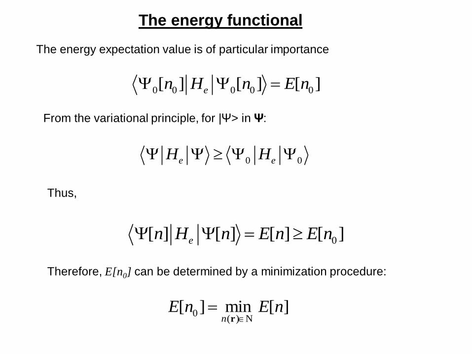
The energy functional
The energy expectation value is of particular importance
0 0 0 0 0[ ] [ ] [ ]en H n E n
From the variational principle, for |Ψ> in Ψ:
0 0e eH H
Thus,
0[ ] [ ] [ ] [ ]en H n E n E n
Therefore, E[n0] can be determined by a minimization procedure:
0( )
[ ] min [ ]n
E n E n
r N


0 0
0 0
0 0
0 0
0 0 0 0
0 0
( ) ( ) ( ) ( )
n e ee eN n e ee eN
n e ee n ext e ee ext
n e ee n e ee
T V V T V V
T V d n V T V d n V
T V T V
r r r r r r

( ) min [ ] ( ) ( )ext
nF n d n V
rr r r


*
2 1 2 2 1 2 2
{ }
( , ) ( , , , ,..., , ) ( , , , ,..., , )e e e e ee N N N N N
s
N d d s s s s s s r r r r r r r r r r

The Kohn-Sham Formulation
Central assertion of KS formulation: Consider a system of Ne
Non-interacting electrons subject to an “external” potential VKS. It
Is possible to choose this potential such that the ground state density
Of the non-interacting system is the same as that of an interacting
System subject to a particular external potential Vext.
A non-interacting system is separable and, therefore, described by a set
of single-particle orbitals ψi(r,s), i=1,…,Ne, such that the wave function is
given by a Slater determinant:
1 1 1
1(x ,..., x ) det[ (x ) (x )]
!e e eN N N
eN
The density is given by
2
1
( ) (x) eN
i i j ij
i s
n
r
The kinetic energy is given by
* 2
1
1 (x) (x)
2
eN
s i i
i s
T d
r


KS
( )( )
( )
xcext
EnV V d
n
r
r rr r r

/ 22
1
1( ) ( )
2
eN
s i i
i
T
r r

Some simple results from DFT
Ebarrier(DFT) = 3.6 kcal/mol
Ebarrier(MP4) = 4.1 kcal/mol

Geometry of the protonated methanol dimer
2.39Å
MP2 6-311G (2d,2p) 2.38 Å

Results methanol
Expt.: -3.2 kcal/mol
Dimer dissociation curve of a neutral dimer
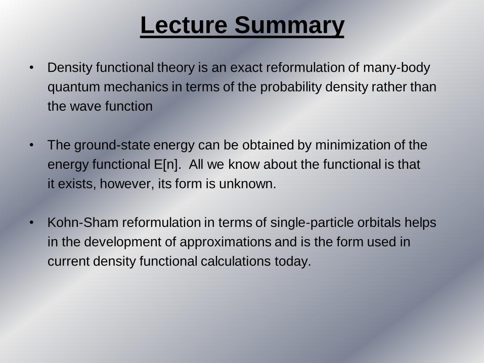
Lecture Summary
• Density functional theory is an exact reformulation of many-body
quantum mechanics in terms of the probability density rather than
the wave function
• The ground-state energy can be obtained by minimization of the
energy functional E[n]. All we know about the functional is that
it exists, however, its form is unknown.
• Kohn-Sham reformulation in terms of single-particle orbitals helps
in the development of approximations and is the form used in
current density functional calculations today.

Get a diamond anvil cell
Get beamtime on a synchrotron
Load your cell.Put medium.
Go to synchrotron
Run your experiment
Get an ab initio software package
Get time on a supercomputer
Input your structure.Choose pseudos, XCs.
Go to supercomputer
Run your experiment
experimental methods computational methods

What is it hard to calculate ?
Transport properties: thermal conductivity, electrical conductivity of insulators, rheology, diffusion
Excited electronic states: optical spectra (=constants?)
Width of IR/Raman peaks, Melting curves, Fluid properties
Electronic properties: orbital energies, chemical bonding, electrical conductivity
Structural properties: prediction of structures (under extreme conditions),
phase diagrams, surfaces, interfaces, amorphous solids
Mechanical properties: elasticity, compressibility, thermal expansion
Dielectric properties: hybridizations, atomic dynamic charges, dielectric susceptibilities,
polarization, non-linear optical coefficients, piezoelectric tensor
Spectroscopic properties: Raman spectra with peak position and intensity, IR peaks
Dynamical properties: phonons, lattice instabilities, prediction of structures, thermodynamic
properties, phase diagrams, thermal expansion
What we can calculate ?

t: Xt Xt (=V) Xt(=A) m
Compute new Fthen F = ma
t+1: Xt+1 Xt+1 Xt+1 m
A set of N particles with masses mn and initial positions Xn

Attractive zoneRepulsive zone
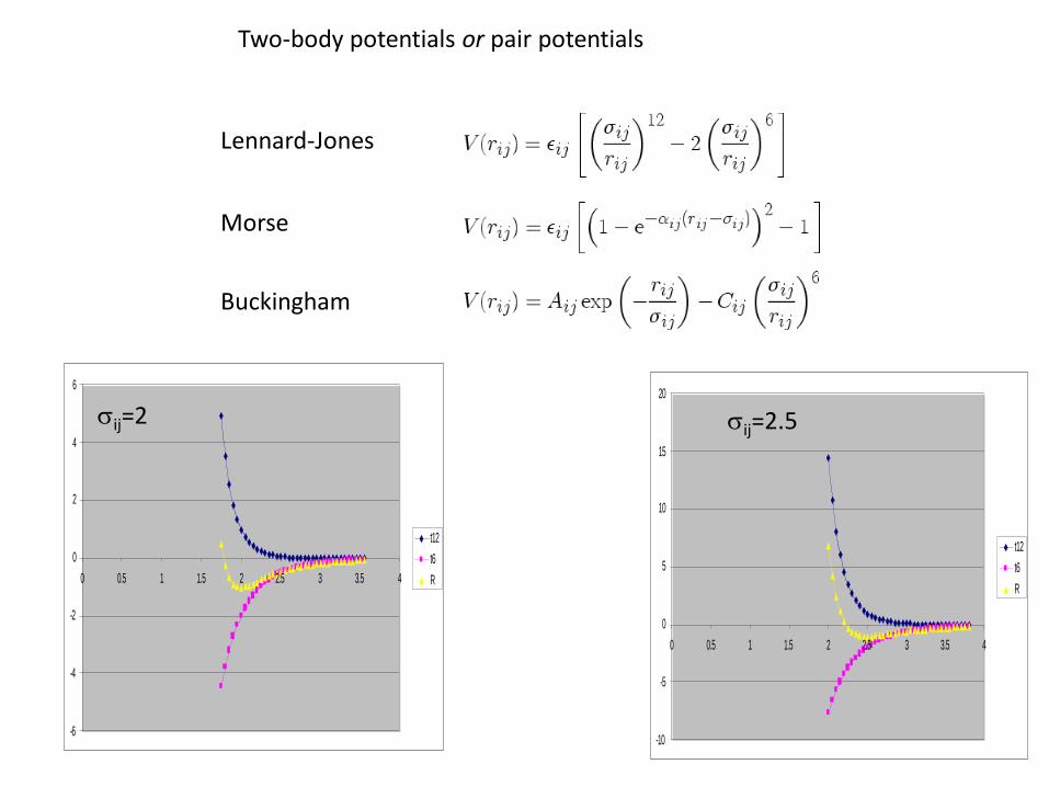
Lennard-Jones
Morse
Buckingham
Two-body potentials or pair potentials
-10
-5
0
5
10
15
20
0 0.5 1 1.5 2 2.5 3 3.5 4
t12
t6
R
sij=2.5
-6
-4
-2
0
2
4
6
0 0.5 1 1.5 2 2.5 3 3.5 4
t12
t6
R
sij=2

Multibody potentials
Vij(rij) = Vrepulsive(rij) + bijkVattractive(rij)
2 body 3+ body

Force fields – very good for molecules
Many other examples:CHARMM, polarizable, valence-bond models,
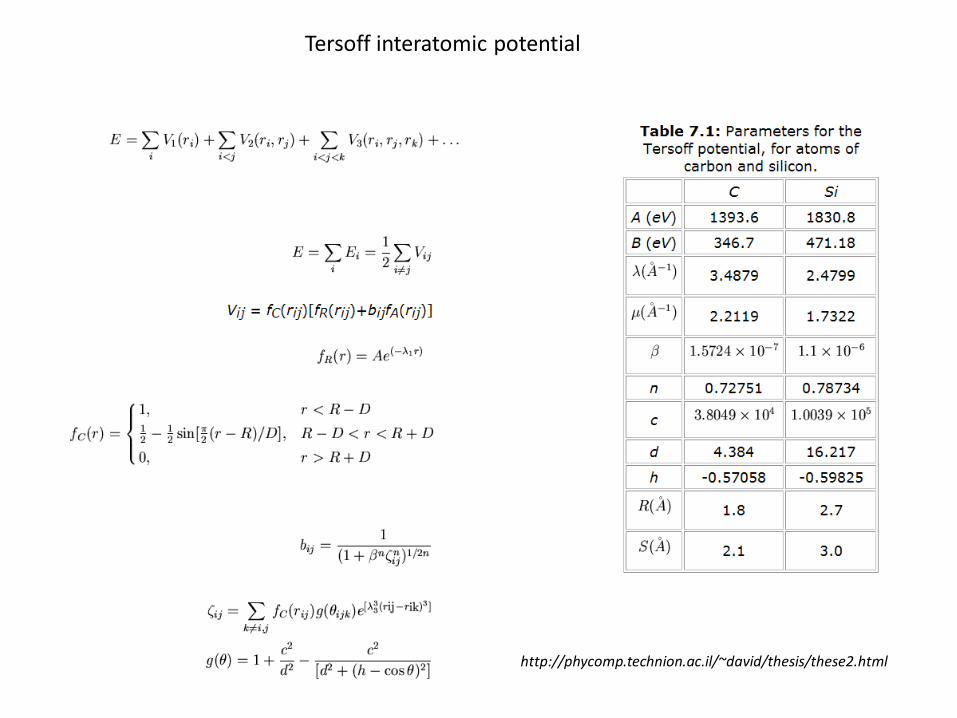
Tersoff interatomic potential
http://phycomp.technion.ac.il/~david/thesis/these2.html

Non-empirical = first-principles or ab initio- the energy is exactly calculated
- no experimental input
+ transferability, accuracy, many properties
- small systems

Schrödinger equation
time-dependent
time-independent
>
¶>= )(|)(|)( t
tittH nn yy
>>=+Ñ- nnn ErUm
yy ||)(2
[ 22
nE Eigenvalues
>ny| Eigenstates

Schrödinger equation involves many-body interactions
Kinetic energy of the electrons
External potential

Wavefunction
>ny| -contains all the measurable information-gives a measure of probability: yyyy *| >=< nn
>ny|~ many-particle wavefunction:
depends on the position of electrons and nucleiscales factorial
For a system like C atom: 6 electrons : 6! evaluations = 720
For a system like O atom: 8 electrons : 8! evaluations = 40320
For a system like Ne atom: 10 electrons: 10! Evaluations = 3628800
For one SiO2 molecule: 30electrons+3nuclei= 8.68E36 evaluations
UNPRACTICAL!

DENSITY FUNCTIONAL THEORY
- What is DFT ?
- Codes
- Planewaves and pseudopotentials
- Types of calculation
- Input key parameters
- Standard output
- Examples of properties:
- Electronic band structure
- Equation of state
- Elastic constants
- Atomic charges
- Raman and Infrared spectra
- Lattice dynamics and thermodynamics
THEORETICAL ASPECTS
PRACTICAL ASPECTS
EXAMPLES

What is DFT
Idea:
one determines the electron density (Kohn, Sham in the sixties: the one responsible
for the chemical bonds) from which by proper integrations and derivations all the
other properties are obtained.
INPUT
Structure: atomic types + atomic positions = initial guess of the geometry
There is no experimental input !

What is DFT
Kinetic energy of non-interacting electrons
Energy term due to exterior
Coulombian energy =Eee + EeN+ ENN
Exchange correlation energy
Decrease Increasesenergy
)]([)]([)]([)]([)]([ rnErnErnErnTrnE xccolexts +++=
Electron spin:
ò ò ò= ),...,,,(),....,,,(...)( 3232
*3
3
3
2
3
NNN rrrrrrrrrdrdrdNrn yy
What is DFT

Exc: LDA vs. GGA
LDA = Local Density ApproximationGGA = Generalized Gradient Approximation
Non-
ò= drrrnE xcxc )()( e ò D= drrrrnE xcxc ),()( e

Flowchart of a standard DFT calculation
Initialize wavefunctions and electron density
Compute energy and potential
Update energy and density
Check convergence
Print required output
)]([)]([)]([)]([)]([ rnErnErnErnTrnE xccolexts +++=
ò ò ò= ),...,,,(),....,,,(...)( 3232
*3
3
3
2
3
NNN rrrrrrrrrdrdrdNrn yy
In energy/potentialIn forcesIn stresses

Crystal structure – non-periodic systems
Point-defect Surface Molecule
“big enough”

Core electrons pseudopotential
Valence electrons computed self-consistently
Input key parameters - pseudopotentials
Semi-core states

All electron wavefunction
Pseudo-wavefunction
Input key parameters - pseudopotentials
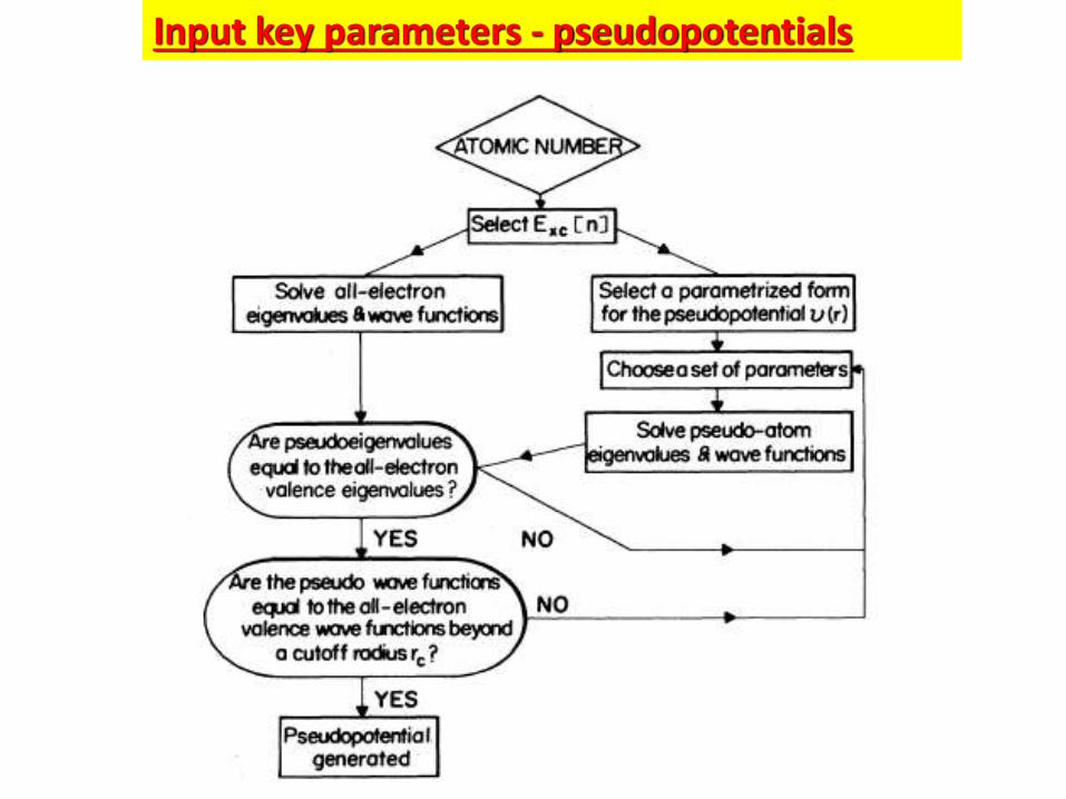
Input key parameters - pseudopotentials

Input key parameters - pseudopotentials
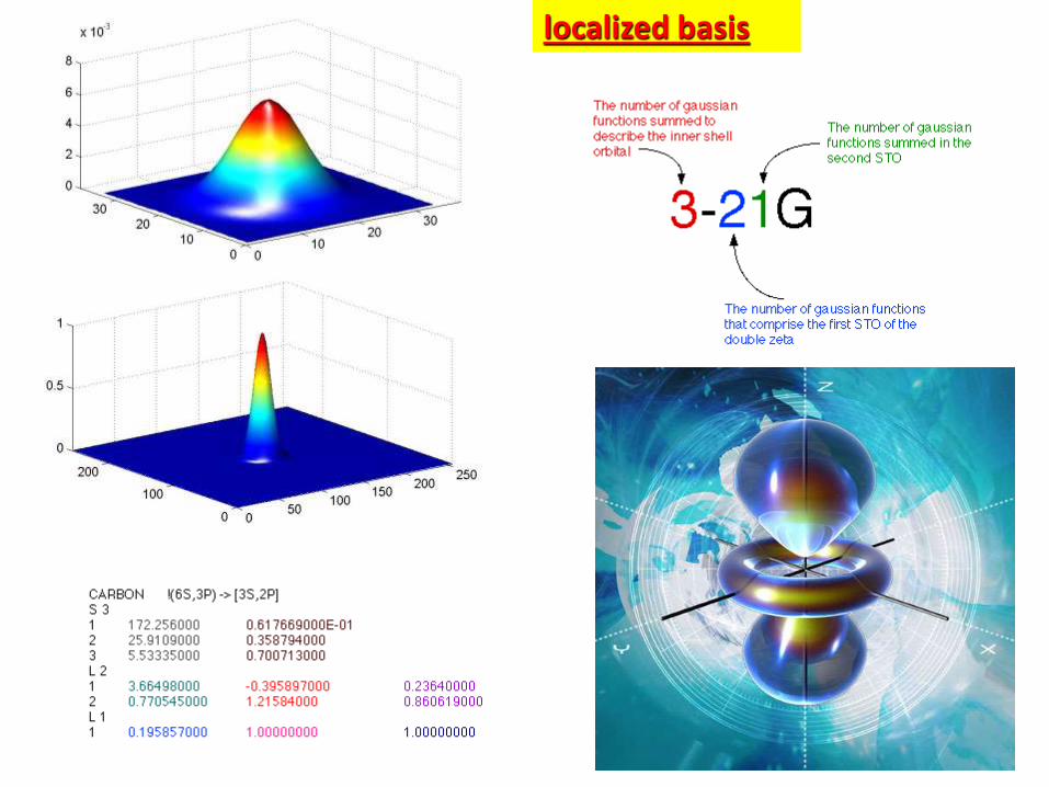
localized basis

Planewaves are characterized by their
wavevector G
angular speed w
wavelength= 2p/G
frequencyf = w/2p
period
T = 1/f = 2p/w
velocityv = /T = w/k
planewaves
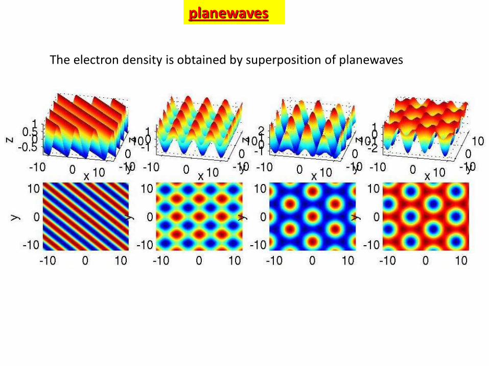
The electron density is obtained by superposition of planewaves
planewaves

Input key parameters - K-points
Limited set of k points ~ boundary conditions

after: http://www.psi-k.org/Psik-training/Gonze-1.pdf

Electronic properties: electronic band structure, orbital energies, chemical bonding,
hybridization, insulator/metallic character, Fermi surface, X-ray diffraction diagrams
Structural properties: crystal structures, prediction of structures under extreme
conditions, prediction of phase transitions, analysis of hypothetical structures
Mechanical properties: elasticity, compressibility
Dielectric properties: hybridizations, atomic dynamic charges, dielectric
susceptibilities, polarization, non-linear optical coefficients, piezoelectric tensor
Spectroscopic properties: Raman and Infrared active modes, silent modes,
symmetry analysis of these modes
Dynamical properties: phonons, lattice instabilities, prediction of structures, study
of phase transitions, thermodynamic properties, electron-phonon coupling
PRACTICAL ASPECTS: Properties

Values of the parameters
How to choose between LDA and GGA ?
- relatively homogeneous systems LDA
- highly inhomogeneous systems GGA
- elements from “p” bloc LDA
- transitional metals GGA
- LDA underestimates volume and distances
- GGA overestimates volume and distances
- best: try both: you bracket the experimental value

Values of the parameters
How to choose pseudopotentials ?
- the pseudopotential must be for the same XC as the calculation
- preferably start with a Troullier-Martins-type
- if it does not work try more advanced schemes
- check semi-core states
- check structural parameters for the compound not element!

Values of the parameters
How to choose no. of planewaves and k-points ?
- check CONVERGENCE of the physical properties

-12.08
-12.075
-12.07
-12.065
-12.06
-12.055
-12.05
-12.045
15 20 25 30 35 40 45 50
Tota
l en
erg
y (H
a)
ecut (Ha)
-50
-45
-40
-35
-30
-25
-20
-15
-10
-5
0
15 20 25 30 35 40 45 50
-P (
GP
a)
ecut (Ha)
Values of the parameters
- check CONVERGENCE of the physical properties

Usual output of calculations (in ABINIT)
Log (=STDOUT) filedetailed information about the run; energies, forces, errors, warnings,etc.
Output file:simplified “clear” output:
full list of run parameterstotal energy; electronic band eigenvalues; pressure; magnetization, etc.
Charge density = DEN
Electronic density of states = DOS
Analysis of the geometry = GEO
Wavefunctions = WFK, WFQ
Dynamical matrix = DDB
etc.
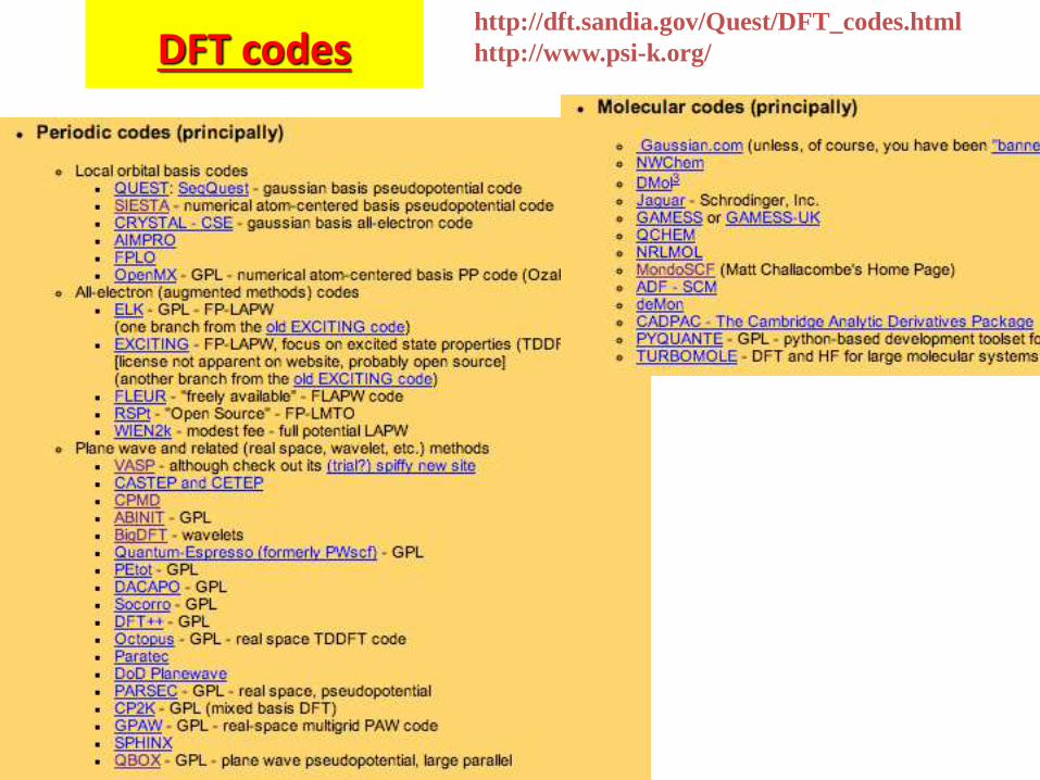
DFT codes http://dft.sandia.gov/Quest/DFT_codes.html
http://www.psi-k.org/

DFT codes:
ABINIT is a package whose main program allows one to find the total energy, charge density and electronic structure of systems made of electrons and nuclei (molecules and periodic solids) within Density Functional Theory (DFT), using pseudopotentials and a planewave basis. ABINIT also includes options to optimize the geometry according to the DFT forces and stresses, or to perform molecular dynamics simulations using these forces, or to generate dynamical matrices, Born effective charges, and dielectric tensors. Excited states can be computed within the Time-Dependent Density Functional Theory (for molecules), or within Many-Body Perturbation Theory (the GW approximation). In addition to the main ABINIT code, different utility programs are provided.
First-principles computation of material properties : the ABINIT software project.X. Gonze, J.-M. Beuken, R. Caracas, F. Detraux, M. Fuchs, G.-M. Rignanese, L. Sindic, M. Verstraete, G. Zerah, F. Jollet, M. Torrent, A. Roy, M. Mikami, Ph. Ghosez, J.-Y. Raty, D.C. Allan
Computational Materials Science, 25, 478-492 (2002)
A brief introduction to the ABINIT software package.X. Gonze, G.-M. Rignanese, M. Verstraete, J.-M. Beuken, Y. Pouillon, R. Caracas, F. Jollet, M. Torrent, G. Zerah, M. Mikami, P. Ghosez, M. Veithen, V. Olevano, L. Reining, R. Godby, G. Onida, D. Hamann and D. C. Allan
Z. Kristall., 220, 558-562 (2005)
A B I N I T

Sequential calculations one processor at a timeParallel calculations several processors in the same time

1 flop = 1 floating point operation / cycle
Itanium 2 @ 1.5 GHz ~ 6Gflops/sec = 6*109 operations/second
These are Gflops / second (~0.5 petaflop)= millions of operations / second


RUN MD CODE

Jmol exercise: http://jmol.sourceforge.net/

EXTRACT RELEVANT INFORMATION:
Atomic positionsAtomic velocitiesEnergyStress tensor
VISUALIZE SIMULATION (ex: jmol, vmd)
PERFORM STATISTICS

Ex: coordination in forsteritic melt at mid-mantle conditions
C-O Si-O

Design of Catalysts and Electrocatalysts:
From DFT Prediction to Experimental Verification
Jingguang Chen
Columbia University & BNL
Email: [email protected]
CFN Workshop, Nov. 5, 2014

Development of Novel Catalysts
• Supported catalysts:
- More relevant to commercial catalysts and processes
- Fast (high throughput) evaluation
- “Heterogeneous” in electronic and catalytic properties
• Single crystal surfaces:
- Atomic level understanding from experiments and theory
- Materials gap: single crystal vs. polycrystalline materials
- Pressure gap: ultrahigh vacuum (UHV: ~10-12 psi)
• Need to bridge “materials gap” and “pressure gap”
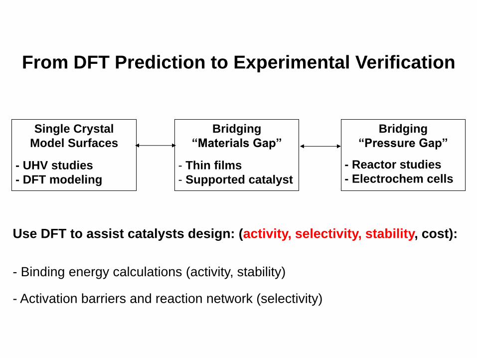
Bridging
“Materials Gap”
- Thin films
- Supported catalyst
Single Crystal
Model Surfaces
- UHV studies
- DFT modeling
Bridging
“Pressure Gap”
- Reactor studies
- Electrochem cells
From DFT Prediction to Experimental Verification
Use DFT to assist catalysts design: (activity, selectivity, stability, cost):
- Binding energy calculations (activity, stability)
- Activation barriers and reaction network (selectivity)

Bridging
“Materials Gap”
- Thin films
- Supported catalyst
Single Crystal
Model Surfaces
- UHV studies
- DFT modeling
Bridging
“Pressure Gap”
- Reactor studies
- Electrochem cells
Examples of DFT prediction and experimental verification:
- Correlating hydrogen binding energy (HBE) with water electrolysis activity
- Correlating hydrogen binding energy (HBE) with hydrogenation activity
- Correlating activation barrier with hydrogenation selectivity
Outline of Presentation

Correlating HBE with Water Electrolysis Activity
Esposito, Hunt & Chen,
Angew. Chem. Int. Ed.
49 (2010) 9859
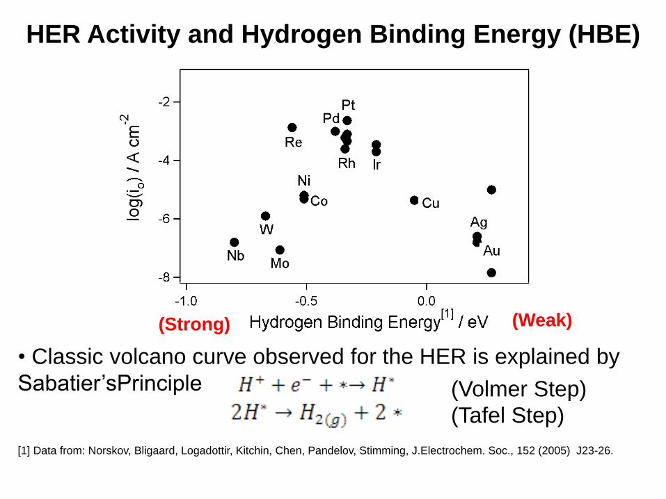
HER Activity and Hydrogen Binding Energy (HBE)
[1] Data from: Norskov, Bligaard, Logadottir, Kitchin, Chen, Pandelov, Stimming, J.Electrochem. Soc., 152 (2005) J23-26.
• Classic volcano curve observed for the HER is explained by
Sabatier’sPrinciple (Volmer Step)
(Tafel Step)
(Weak) (Strong)
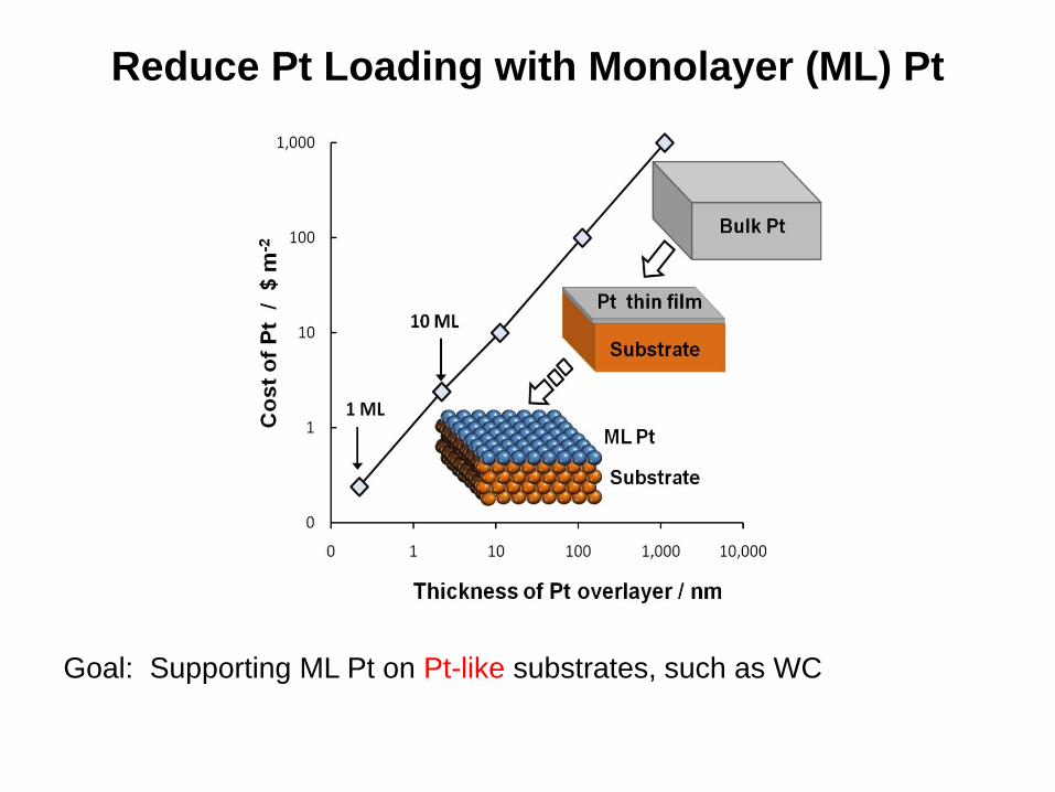
Reduce Pt Loading with Monolayer (ML) Pt
Goal: Supporting ML Pt on Pt-like substrates, such as WC

Surface HBE (eV)
WC(001) -0.99
Pt(111) -0.46
1 ML Pt-WC(001) -0.43
DFT-calculated per-atom hydrogen
binding energy (HBE) for WC, Pt, and 1
ML Pt-WC surfaces with a hydrogen
coverage of 1/9 ML.
d-band density of states
DFT Prediction: Similar HBE Values between
Monolayer Pt-WC and Bulk Pt
Pt WC
1 atomic
layer of Pt

Experimental Verification of Activity and Stability
HER Activity of 1 ML Pt/WC approaches to that of Pt foil
Esposito, Hunt, Birmire & Chen, Angew. Chem. Int. Ed. 49 (2010) 9859

DFT Prediction of Stability of Pt/WC and Pt/C
• Use DFT to compare adhesion of Pt atoms to WC and Pt surfaces:
Pt-(Substrate) > Pt-Pt
Pt-(Substrate) < Pt-Pt
ML configuration
favored
Particles
favored
Binding Energy Outcome
Pt
migration
ML surface atoms Substrate Binding energy
/ eV
(M-X^) - (M-M) BE
/ eV
Pt
Pt(111) -5.43 0.00
C(0001) -4.12 1.31
WC(0001) -6.59 -1.16
W2C(0001) -6.51 -1.08

Experimental Verification of HER Stability
• No change in overpotential observed with time
• No change in LSV before and after CP
• XPS and SEM measurements confirmed stability
Chronopotentiometry Linear Sweep Voltammetry
Esposito, Hunt & Chen, J. Am. Chem. Soc. 134 (2012) 3025

Other ML/TMC Electrocatalysts for HER in Acid
Volcano relationship provides design principles of electrocatalysts
Kimmel , Yang & Chen, J. Catalysis, 312 (2014) 216
Hydrogen binding energy (eV)
log [
HE
R e
xchange c
urr
ent
density (
A c
m-2
)]

HER Catalysts in Alkaline Environment
Volcano relationship also appears to hold in alkaline electrolyte
Sheng et al. Energy & Env. Sci. 6 (2013) 1509

Bridging
“Materials Gap”
- Thin films
- Supported catalyst
Single Crystal
Model Surfaces
- UHV studies
- DFT modeling
Bridging
“Pressure Gap”
- Reactor studies
- Electrochem cells
Examples of DFT prediction and experimental verification:
- Correlating hydrogen binding energy (HBE) with water electrolysis activity
- Correlating hydrogen binding energy (HBE) with hydrogenation activity
- Correlating activation barrier with hydrogenation selectivity
Outline of Presentation

Monolayer Bimetallic Surfaces
Surface Monolayer Subsurface Monolayer
Surface Alloy
Modified surface chemical properties due to:
–Ligand effect – electronic configuration
–Compressive and tensile strain - lattice mismatch

DFT Prediction of HBE Values
Hydrogen binding energy (HBE) can be controlled by surface structures
Kitchin, Norskov, Barteau & Chen, Phys. Rev. Lett. 93 (2004) 156801
Murillo, Goda & Chen, J. Am. Chem. Soc. 129 (2007) 7101
-340
-320
-300
-280
-260
-240
-220
Hyd
rog
en
Bin
din
g E
ne
rgy
(k
J/m
ol)
-3.5 -3.0 -2.5 -2.0 -1.5 -1.0
d-band center (eV)
Pt-Fe-Pt
Pt-Co-PtPt-Ni-Pt
Pt-Cu-Pt
Pt(111)
Cu(111)
Cu-Pt-Pt
Ni-Pt-Pt
Fe-Pt-Pt
Co-Pt-Pt
Co(0001)
Ni(111)

Controlling Hydrogenation Activity: Correlating with Binding Energy
Low-Temperature Cyclohexene Hydrogenation:
Assumption for Higher Hydrogenation Activity:
• Weakly bonded H atoms
• Weakly bonded cyclohexene
Ni/Pt
HH

-80
-60
-40
-20
0
Cyc
loh
ex
en
e B
ind
ing
En
erg
y (
kJ
/mo
l)
-3.0 -2.5 -2.0 -1.5 -1.0
d-band center (eV)
Pt-Fe-Pt
Pt-Co-Pt
Pt-Ni-Pt
Pt-Cu-PtNi(111)
Pt(111)
Ni-Pt-Pt
DFT Calculations of Binding Energies of
Hydrogen and Cyclohexene
BE values follow the same trend: Ni-Pt(111) > Ni ~ Pt > Pt-Ni-Pt(111)
-340
-320
-300
-280
-260
-240
-220
Hyd
rog
en
Bin
din
g E
ne
rgy
(k
J/m
ol)
-3.5 -3.0 -2.5 -2.0 -1.5 -1.0
d-band center (eV)
Pt-Fe-Pt
Pt-Co-PtPt-Ni-Pt
Pt-Cu-Pt
Pt(111)
Cu(111)
Cu-Pt-Pt
Ni-Pt-Pt
Fe-Pt-Pt
Co-Pt-Pt
Co(0001)
Ni(111)

Low-Temperature Hydrogenation of
Cyclohexene Due to Weakly Bonded H
- Weakly bonded M-H leads to low-T hydrogenation
+ H
M
Inte
ns
ity
(a
rb.
un
its
)
600500400300200
Temperature (K)
Pt-Ni-Pt(111)
Ni-Pt-Pt(111)
Ni(111) Film
Cyclohexane (84 amu)
203 K
171 K
Pt(111)

Binding Energies Correlate with
Cyclohexene Hydrogenation Activity
Sabatier’s principle: not too strong, not too weak!
Volcano relationship allows prediction of hydrogenation activity
0.035
0.030
0.025
0.020
0.015
0.010
0.005
0.000Hyd
rog
en
ati
on
Acti
vit
y (
mo
lecu
les /
meta
l ato
m)
-150 -100 -50 0
Cyclohexene Binding Energy (kJ/mol)
Ni-Pt-Pt
Pt(111) Pt-Co-Pt
Pt-Fe-Pt
Pt-Ni-Pt
Pt/W(110)Fe-Pt-Pt
Inte
nsit
y (
arb
. u
nit
s)
600500400300200Temperature (K)
Pt(111)
Pt-Co-Pt(111)
180 K
203 K
187 K
Pt-Fe-Pt(111)
Pt-Ni-Pt(111)
Pt-Cu-Pt(111)
Cyclohexane (84 amu)

DFT Prediction of Stable Bimetallic Structures
21
General Stability includes:
Admetals – 3d, 4d, 5d
Host metals – Ni, Pd, Pt
Vacuum
0.5 ML H
0.5 ML O
Menning & Chen,
J. Chem. Phys, 130 (2009) 174709

Experimental Verification of Bimetallic Structures
Coordination
Number 10% H2 at 50 °C—NiPt/C
Experimental Simulation
Pt-Pt 1.9 ± 0.8 2.696 ± 0.003
Pt-Ni 3.5 ± 0.4 3.904 ± 0.007
Coordination
Number 10% H2 at 225 °C—NiPt/C
Experimental Simulation
Pt-Pt 2.0 ± 0.7 2.675 ± 0.005
Pt-Ni 3.8 ± 0.3 4.148 ± 0.008
Coordination
Number APR at 225 °C—NiPt/C
Experimental Simulation
Pt-Pt 6.0 ± 1.4 4.429 ± 0.006
Pt-Ni 1.9 ± 0.8 2.24 ± 0.03
Tupy, Karim, Vlachos, Chen, ACS Catalysis, 2 (2012) 2290
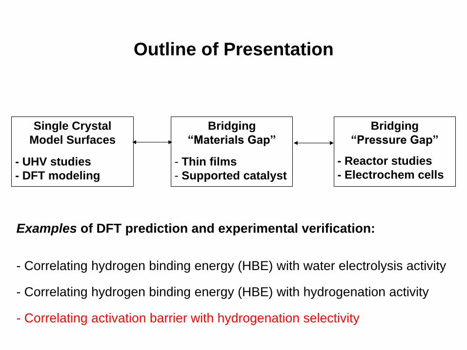
Bridging
“Materials Gap”
- Thin films
- Supported catalyst
Single Crystal
Model Surfaces
- UHV studies
- DFT modeling
Bridging
“Pressure Gap”
- Reactor studies
- Electrochem cells
Examples of DFT prediction and experimental verification:
- Correlating hydrogen binding energy (HBE) with water electrolysis activity
- Correlating hydrogen binding energy (HBE) with hydrogenation activity
- Correlating activation barrier with hydrogenation selectivity
Outline of Presentation

Selective Hydrogenation Requires More
Complicated DFT Calculations
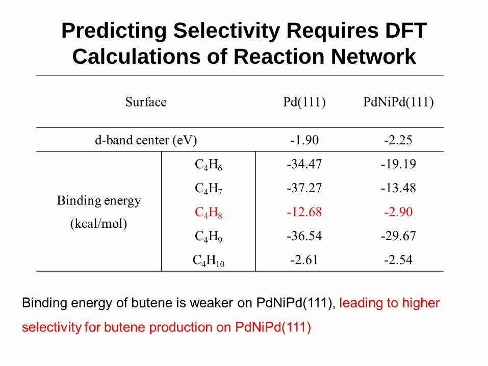
Predicting Selectivity Requires DFT
Calculations of Reaction Network

Experimental Verification on Model Surfaces

Batch Reactor: Hydrogenation Activity
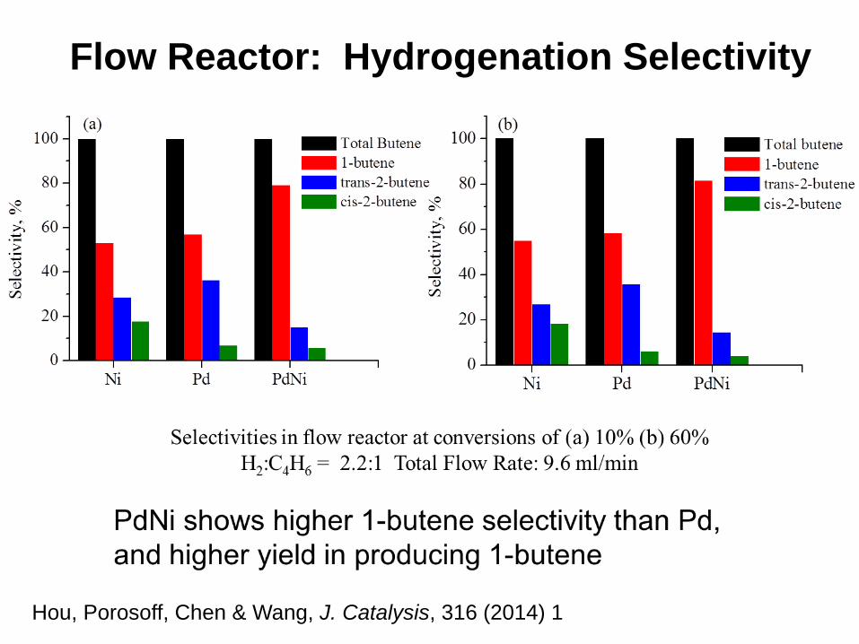
Flow Reactor: Hydrogenation Selectivity
Hou, Porosoff, Chen & Wang, J. Catalysis, 316 (2014) 1

Conclusions
• Bimetallic and carbide catalysts offer the advantages of
reduced cost and enhanced activity, selectivity and stability
• Combined theory, surface science, and catalytic studies are
critical in design of novel catalytic materials
Bridging
“Materials Gap”
- Thin films
- Supported catalyst
Single Crystal
Model Surfaces
- UHV studies
- DFT modeling
Bridging
“Pressure Gap”
- Reactor studies
- Electrochem Cell
Review: Yu, Porosoff & Chen, “Review of Pt-based Bimetallic Catalysis: From
Model Surfaces to Supported Catalysts”, Chemical Reviews, 112 (2012) 5780