Dense Linear Algebra on DistributedHeterogeneous Hardware with a Symbolic DAG

Approach

George Bosilca Aurelien Bouteiller Anthony DanalisThomas Herault Piotr Luszczek Jack J. Dongarra

January 24, 2012

1 Introduction and MotivationAmong the various factors that drive the momentous changes occurring in the designof microprocessors and high end systems [1], three stand out as especially notable:

1. the number of transistors per chip will continue the current trend, i.e. doubleroughly every 18 months, while the speed of processor clocks will cease to in-crease;

2. the physical limit on the number and bandwidth of the CPUs pins is becoming anear-term reality;

3. a strong drift toward hybrid/heterogeneous systems for petascale (and larger)systems is taking place.

While the first two involve fundamental physical limitations that current technologytrends are unlikely to overcome in the near term, the third is an obvious consequenceof the first two, combined with the economic necessity of using many thousands ofcomputational units to scale up to petascale and larger systems.

More transistors and slower clocks require multicore designs and an increased par-allelism. The fundamental laws of traditional processor design – increasing transistordensity, speeding up clock rate, lowering voltage – have now been stopped by a set ofphysical barriers: excess heat produced, too much power consumed, too much energyleaked, and useful signal overcome by noise. Multicore designs are a natural evolu-tionary response to this situation. By putting multiple processor cores on a single die,architects can overcome the previous limitations, and continue to increase the num-ber of gates per chip without increasing the power densities. However, since excessheat production means that frequencies cannot be further increased, deep-and-narrowpipeline models will tend to recede as shallow-and-wide pipeline designs become thenorm. Moreover, despite obvious similarities, multicore processors are not equiva-lent to multiple-CPUs or to SMPs. Multiple cores on the same chip can share various

1

caches (including TLB – Translation Look-aside Buffer) while competing for memorybandwidth. Extracting performance from such configurations of resources means thatprogrammers must exploit increased thread-level parallelism (TLP) and efficient mech-anisms for inter-processor communication and synchronization to manage resourceseffectively. The complexity of fine grain parallel processing will no longer be hid-den in hardware by a combination of increased instruction level parallelism (ILP) andpipeline techniques, as it was with superscalar designs. It will have to be addressed atan upper level, in software, either directly in the context of the applications or in theprogramming environment. As code and performance portability remain essential, theprogramming environment has to drastically change.

A thicker memory wall means that communication efficiency becomes crucial. Thepins that connect the processor to main memory have become a strangle point, which,with both the rate of pin growth and the bandwidth per pin slowing down, is not flatten-ing out. Thus the processor to memory performance gap, which is already approachinga thousand cycles, is expected to grow by 50% per year according to some estimates.At the same time, the number of cores on a single chip is expected to continue todouble every 18 months, and since limitations on space will keep the cache resourcesfrom growing as quickly, cache per core ratio will continue to diminish. Problems withmemory bandwidth and latency, and cache fragmentation will, therefore, tend to be-come more severe, and that means that communication costs will present an especiallynotable problem. To quantify the growing cost of communication, we can note that timeper flop, network bandwidth (between parallel processors), and network latency are allimproving, but at significantly different rates: 59%/year, 26%/year and 15%/year, re-spectively [2]. Therefore, it is expected to see a shift in algorithms’ properties, fromcomputation-bound, i.e. running close to peak today, toward communication-boundin the near future. The same holds for communication between levels of the mem-ory hierarchy: memory bandwidth is improving 23%/year, and memory latency only5.5%/year. Many familiar and widely used algorithms and libraries will become ob-solete, especially dense linear algebra algorithms which try to fully exploit all thesearchitecture parameters. They will need to be reengineered and rewritten in order tofully exploit the power of the new architectures.

In this context, the PLASMA project [3] has developed new algorithms for denselinear algebra on shared memory systems based on tile algorithms. Widening the scopeof these algorithms from shared to distributed memory, and from homogeneous archi-tectures to heterogeneous ones, has been the focus of a follow-up project, DPLASMA.DPLASMA introduces a novel approach to schedule dynamically dense linear alge-bra algorithms on distributed systems. Similarly to PLASMA, to whom it shares mostof the mathematical algorithms, it is based on tile algorithms, and takes advantageof DAGUE [4], a new generic distributed Direct Acyclic Graph Engine for high per-formance computing. The DAGUE engine features a DAG representation indepen-dent of the problem-size, overlaps communications with computation, prioritizes tasks,schedules in an architecture-aware manner and manages micro-tasks on distributed ar-chitectures featuring heterogeneous many-core nodes. The originality of this engineresides in its capability to translate a sequential nested-loop code into a concise andsynthetic format which it can interpret and then execute in a distributed environment.We consider three common dense linear algebra algorithms, namely: Cholesky, LU and

2

QR factorizations, part of the DPLASMA library, to investigate through the DAGUEframework their data driven expression and execution in a distributed system. It hasbeen demonstrated, through performance results at scale, that this approach has thepotential to bridge the gap between the peak and the achieved performance that is char-acteristic in the state-of-the-art distributed numerical software on current and emergingarchitectures. However, one of the most essential contributions, in our view, is the sim-plicity with which new algorithmic variants may be developed and how they can beported to a massively parallel heterogeneous architecture without much consideration,at the algorithmic level, of the underlying hardware structure or capabilities. Due tothe flexibility of the underlying DAG scheduling engine and the powerful expression ofparallel algorithms and data distributions, the DAGUE environment is able to deliver asignificant percentage of the peak performance, providing a high level of performanceportability.

2 Distributed Dataflow by Symbolic EvaluationEarly in the history of computing, Direct Acyclic Graphs (DAG) have been used toexpress the dependencies between the inputs and outputs of a program’s tasks [5].By following these dependencies, tasks whose datasets are independent (i.e. respectthe Bernstein conditions [6]) can be discovered, hence enabling parallel execution.The dataflow execution model [7] is iconic of DAG based approaches; although it hasproved very successful for grid and peer-to-peer systems [8, 9], in the last two decades,it generally suffered on other HPC system types, generally because the hardware trendsfavored the Single Program, Multiple Data (SPMD) programming style with massivebut uniform architectures.

Recently, the advent of multicore processors has been undermining the dominanceof the SPMD programming style, reviving interest in the flexibility of dataflow ap-proaches. Indeed, several projects [10, 11, 12, 13, 14], mostly in the field of LinearAlgebra, have proposed to revive the general use of DAGs, as an approach to tacklethe challenges of harnessing the power of multi-core and hybrid platforms. However,these recent projects have not considered the context of distributed memory environ-ments, with a massive number of many-core compute nodes clustered in a single sys-tem. In [15], an implementation of a tiled algorithm based on dynamic schedulingfor the LU factorization on top of UPC is proposed. [16] uses a static scheduling ofthe Cholesky factorization on top of MPI to evaluate the impact of data representationstructures. All of these projects address a single problem and propose ad-hoc solutions;there is clearly a need for a more ambitious framework to enable expressing a largervariety of algorithms as dataflow and execute them on distributed systems.

Scheduling DAGs on clusters of multi-cores introduces new challenges: the sched-uler should be dynamic to address the non determinism introduced by communications;and in addition to the dependencies themselves, data movements must be tracked be-tween nodes. Evaluation of dependencies must be carried in a distributed, problem sizeand system size independent manner: the complexity of the scheduling has to be di-vided by the number of nodes to retain scalability at large scale, which is not the case inmany previous works which unroll the entire DAG on every compute node. Although

3

dynamic and flexible scheduling is necessary to harness the full power of many-corenodes, network capacity is the scarcest resource, meaning that the programmer shouldretain control of the communication volume and pattern.

2.1 Symbolic EvaluationThere are three general approaches to building and managing the DAG during the ex-ecution. The first approach is to describe the DAG itself, as a potentially cyclic graph,whose set of vertices represents the tasks whose edges represent the data access de-pendencies. Each vertex and edge of the graph are parameterized, and represent manypossible tasks. At runtime, that concise representation is completely unrolled in mem-ory, in order for the scheduling algorithm to select an ordering of the tasks that doesnot violate causality. The tasks are then submitted in order on the resources, accordingto the resulting scheduling [9]. The main drawback of this approach lies in the memoryconsumption associated with the complete unrolling of the DAG. Many algorithms arerepresented by DAGs that hold a huge number of tasks: the Dense Linear Algebra Fac-torizations that we use in this chapter to illustrate the DAGUE engine have a numberof tasks in O(n3), when the problem is of size n.

The second approach is to explore the DAG according to the control flow depen-dency ordering given by a sequential solution to the problem [17, 12, 18, 14]. Thesequential code is modified with pragmas, to isolate tasks that will be run as atomicentities. Every compute node then executes the sequential code in order to discoverthe DAG by following the sequential control flow, and adding dynamic detection ofthe data dependency, allowing for the scheduling of tasks in parallel. Optionally, theseengines use bounded buffers of tasks to limit the impact of the unrolling operation inmemory. The depth of the unrolling decides the number of potential pending tasks, andhas a direct impact on the degree of freedom of the scheduler to find the best matchedtask to be scheduled. One of the central drawbacks of this approach is that a boundedbuffer of tasks limits the exploration of potential parallelism according to the controlflow ordering of the sequential code. Hence, it is a mixed control/data-flow approach,which is not as flexible as a true dataflow approach.

The third approach consists of using a concise, symbolic representation of the DAGat runtime. Using structures such as a Parameterized Task Graph (PTG) proposed in[19], the memory used for DAG representation is linear in the number of task types andtotally independent of the total number of tasks. At runtime, there is no need to unrollthe complete DAG, which can be explored in any order, in any direction (following atask successors, or finding a task predecessors), independently of the control flow. Sucha structure has been considered in [20, 21], where the authors propose a centralizedapproach to schedule computational Linear Algebra tasks on clusters of SMPs using aPTG representation and RPC calls.

In contrast, our approach, in DAGUE, leverages the PTG representation to evaluatethe successors of a given task in a completely decentralized, distributed fashion. TheIN and OUT dependencies, are accessible between any pair of tasks that have a depen-dent relation, in the successor or predecessor direction. If the task A modifies a data dAand passes it to task B, task A can compute that task B is part of its successors simply byinstantiating the parameters in the symbolic expression representing the dependencies

4

of A; task B can compute that task A is part of its predecessors in the same way; andboth tasks know what access type (read-write, read-only) the other tasks uses on thedata on this edge. Indeed, the knowledge of the IN and OUT dependencies, accessibleanywhere in the DAG execution, thanks to the symbolic representation of edges, is suf-ficient to implement a fully distributed scheduling engine. Each node of the distributedsystem evaluates the successors of tasks that it has executed, only when that task com-pleted. Hence, it never evaluates parts of the DAG pertaining to tasks executing onother resources, sparing memory and compute cycles. Not only does the symbolic rep-resentation does allow the internal dependence management mechanism to efficientlycompute the flow of data between tasks without having to unroll the whole DAG, but italso enables to discover the communications required to satisfy remote dependencies,on the fly, without a centralized coordination.

As the evaluation does not rely on the control-flow, the concept of algorithmic look-ing variants, as seen in many factorization algorithms of LAPACK and ScaLAPACKbecomes irrelevant: instead of hard-coding a particular variant of tasks ordering, suchas right-looking, left-looking or top-looking [22], the execution is now data-driven, thetasks to be executed are dynamically chosen based on the resource availabilities. Theissue of which “looking” variant to choose is avoided because the execution of a taskis scheduled when the data is available, rather than relying on the unfolding of the se-quential loops, which enables a more dynamic and flexible scheduling. However, mostprogrammers are not used to think about the algorithm as a DAG. It is oftentimes dif-ficult for the programmer to infer the appropriate symbolic expressions that depict theintended algorithm. We will describe in section 4 how, in most cases, the symbolic rep-resentation can be simply and automatically extracted from decorated sequential code,akin to the more usual input used in code-flow based DAG engines, such as StarPU [14]and SMPSS [17]. We will then illustrate, by using the example of the QR factoriza-tion, the exact steps required from a linear algebra programmer to achieve outstandingperformance on clusters of distributed heterogeneous resources, using DAGUE.

2.2 Task Distribution and Dynamic SchedulingBeyond the evaluation of the DAG itself, there are a number of major principles thatpertain to scheduling tasks on a distributed system. A major consideration is towarddata transfers across distributed resources, in other terms distribution of tasks acrossnodes and the fulfillment of remote dependencies. In many, previously cited, relatedprojects, messaging is still explicit; the programmer has to insert either communica-tion tasks in the DAG, or insert sends and receives in the tasks themselves. As eachcomputing node is working in its own DAG, this is equivalent to coordinating with theother DAGs using messages. This approach limits the degree of asynchrony that canbe achieved by the DAG scheduling, as sends and receives have to be posted at similartime periods to avoid messaging layer resource exhaustion. Another issue is that thecode tightly couples the data distribution and the algorithm. Should one decide for anew data distribution, many parts of the algorithm pertaining to communication taskshave to be modified to fit that new communication pattern.

In DAGUE, the application programmer is relieved from the low-level manage-ment: data movements are implicit, and it is not necessary to specify how to implement

5

the communications; they automatically overlap with computations; all computing re-sources (cores, accelerators, communications) of the computing nodes are handled bythe DAGUE scheduler. The application developer has only to specify the data distri-bution as a set of immutable computable conditions. The task mapping across nodesis then mapped to the data distribution, resulting in a static distribution of tasks acrossnodes. This greatly alleviates the burden of the programmer who faces the complexand concurrent programming environments required for massively parallel distributed-memory machines, while leaving the programmer the flexibility to address complexissues, like load balancing and communication avoidance, that are best addressed byunderstanding the algorithms.

This static task distribution across nodes does not mean that the overall schedulingis static. In a static scheduling, an ordering of tasks is decided offline (usually by con-sidering the control flow of the sequential code), and resources execute tasks by strictlyfollowing that order. On the contrary, a dynamic scheduling is decided at runtime,based on current occupation of local resources. Besides the static mapping of taskson nodes, the order in which tasks are executed is completely dynamic. Because thesymbolic evaluation of the DAG enables implicit remote dependency resolution, nodesdo not need to make assumptions about the ordering of tasks on remote resources tosatisfy the tight coupling of explicit send-receive programs. As a consequence, the or-dering of tasks, even those whose dependencies cross node boundaries, is completelydynamic, and depends only on reactive scheduling decisions based on current networkcongestion and the resources available at the execution location.

When considering the additional complexity introduced by non uniform memoryhierarchies of many-core nodes and the heterogeneity from accelerators, and the desirefor performance portability, it become clear that the scheduling must feature asyn-chrony and flexibility deep at its core. One of the key principles in DAGUE is thedynamic scheduling and placement of tasks within node boundaries. As soon as aresource is idling, it tries to retrieve work from other neighboring local resources in ajob-stealing manner. Scheduling decisions pertaining not only to task ordering, but alsoto resource mapping are hence completely dynamic. The programmer is relieved fromthe intricacies of the hardware hierarchies, his major role is to describe an efficientalgorithm capable of expressing a high level of parallelism, and to let the DAGUEruntime take advantage of the computing capabilities of the machine and solve loadimbalances that appear within nodes, automatically.

3 The DAGUE Dataflow RuntimeThe DAGUE engine has been designed for efficient distributed computing, and hasmany appealing features when considering distributed-memory platforms with hetero-geneous multicore nodes:

1. a symbolic dataflow representation that is independent of the problem-size,

2. automatic extraction of the communication from the dependencies,

3. overlapping of communication and computation,

6

4. task prioritization,

5. and architecture-aware scheduling and management of tasks.

3.1 Intra-node Dynamic Scheduling

0

5

10

15

20

25

GE

MM

du

ratio

n (

ms)

Duration of each individual GEMM operationin a dpotrf 10,000x10,000 run on 48 cores (one node)

(sorted by duration of the operation)

Global DequeueLocal Hierarchical Queues

Figure 1: Duration of each indi-vidual GEMM operation in a dpotrf10,000x10,000 run on 48 cores (sortedby duration of the operation)

From a technical point of view, the schedul-ing engine is distributively executed by all thecomputing resources (nodes). Its main goalis to select a local ready task for which allthe IN dependencies are satisfied, i.e. thedata is available locally, and then execute thebody of the task on the core currently run-ning the scheduling algorithm, or on the ac-celerator serving this core, in the case of anaccelerated-enabled kernel. Once executed,the core returns in the scheduler, and releasesall the OUT dependencies of this task, thuspotentially making more tasks available to bescheduled, locally or remotely. It is notewor-thy to mention that the scheduling mechanismis architecture aware, taking into account not only the physical layout of the cores, butalso the way different cache levels and memory nodes are shared between the cores.This allows the runtime to determine the best local task, i.e. the one that minimizes thenumber of cache misses and data movements over the memory bus.

Task selection (from a list of ready to be executed tasks) is guided by a generalheuristic: data locality, and a user-level controlled parameter: soft priority. The data lo-cality policy allows the runtime to decrease the pressure on the memory bus, by takingadvantage of the cache locality. In Figure 1, two different policies of ready tasks man-agement are analyzed in order to identify their impact on the task duration. The globaldequeue approach manages all ready tasks in a global dequeue, shared by all threads;while the local hierarchical queue manages the ready tasks using queues shared amongthreads based on their distance to particular levels of memory. One can see the slightincrease in the duration of the GEMM tasks when the global dequeue is used; partiallydue to the increased level of cache sharing between ready tasks temporarily close toeach other that get executed on cores without far apart memory sharing. In same timethe user-defined priority is a critical component for driving the DAG execution as closeas possible to the critical path, ensuring a constant high degree of parallelism whileminimizing the possible starvations.

3.2 Communication, and Data Distribution in DAGUEThe DAGUE engine is responsible for moving data from one node to another whennecessary. These data movements are necessary to release dependencies of remotetasks.

7

The communication engine uses a type qualifier called modifier, to define the mem-ory layout touched by a specific data movement. Such a modifier can be expressed asMPI data types, or other types of memory layout descriptors. It informs the commu-nication engine of the shape of the data to be transferred from one memory locationto another, potentially remote, memory location. The application developer is respon-sible for describing the type of data (by providing the above mentioned modifier foreach data flow). At runtime, based on the data distribution, the communication en-gine will move the data transparently using the modifiers. The data tracking engine(described below) is capable of understanding if the different data types overlap, andbehaves appropriately when tracking the dependencies.

The communication engine exhibits a strong level of asynchrony in the progressionof network transfers to achieve communication/computation overlap and asynchronousprogress of tasks on different nodes. For that purpose, in DAGUE, communicationsare handled by a separate dedicated thread, which takes commands from all the otherthreads and issues the corresponding network operations. This thread is usually notbound on a specific core, the operating system schedules this oversubscribed threadby preempting computation-intensive threads when necessary. However, on some spe-cific environments, due to operating system or architectural discrepancies, dedicatinga hardware thread to the communication engine has been proved beneficial.

Upon completion of a task, the dependence resolution is executed. Local tasksactivations are handled locally, while a task completion message is sent to processescorresponding to remote dependencies. Due to the asynchrony of the communicationengine, the network congestion status does not influence the local scheduling. Thus,compute threads are able to focus on the next available compute task as soon as possiblein order to maximize communication/computation overlap.

A task completion message contains information about the task that completed, touniquely identify which task completed, and consequently to determine which databecame available. Task completion messages targeting the same remote process canbe coalesced, and then a single command is sent to each destination process. Thesuccessor relationship is used to build the list of processes that run tasks depending onthe completed task, and these processes are then notified. The communication topologyis adapted to limit the outgoing degree of one-to-all dependencies and establish propercollective communication techniques, such as pipelining or spanning three approaches.

Upon the arrival of a task completion message, the destination process schedulesthe reception of the relevant output data from the parent task by evaluating, in its com-munication thread, the dependencies of the remote completed task. A control messageis sent to the originating process to initiate the data transfers; all output data neededby the destination are received by different rendezvous messages. When one of thedata transfers completes, the receiver invokes locally the dependence resolution func-tion associated with the parent task, inside the communication thread, to release thedependencies related to this particular transfer. Remote dependencies resolutions aredata specific, not task specific, in order to maximize asynchrony. Tasks enabled duringthis process are added to the queue of the first compute thread, as there are no cacheconstraints involved.

In the current version, the communications are performed using MPI. To increaseasynchrony, data messages are non-blocking, point-to-point operations allowing tasks

8

CPU

GPU

core0

core1

stream0

stream1

TaTb Ta

Ta

Tb TbS S S S

S GPU Ta

Tb

TbTb TbTb

Tb Tb

Tb

Tb

in in

out

out

outTb

Figure 2: Schematic (not to scale) DAGUE execution, on a GPU enabled system;kernels Ta and Tb alternate with scheduling actions (S) and in/out GPU asynchronousmemory accesses.

to concurrently release remote dependencies, while keeping the maximum number ofconcurrent messages limited. The collaboration between the MPI processes is real-ized using control messages: short messages containing only the information aboutcompleted tasks. The MPI process pre-posts persistent receives to handle the controlmessages for the maximum number of concurrent task completions. Unlike the datamessages, there is no limit to the number of control messages that can be sent, to avoiddeadlocks. This can generate unexpected messages, but only for small size messages.Due to the rendezvous protocol described in the previous paragraph, the data payloadsare never unexpected, thus reducing memory consumption from the network engineand ensuring flow control.

3.3 Accelerator SupportAccelerators computing units feature tremendous computing power, but at the expenseof supplementary complexity. In large multicore nodes, load balance between the hostCPU cores and the accelerators is paramount to reach a significant portion of the peakcapacity of the entire node. Although accelerators usually require explicit movementsof data to offload computation to the device, considering them as mere ”remote” unitswould not yield satisfactory results. The large discrepancy between the performanceof the accelerators and the host cores renders any attempt at defining an efficient staticload balance difficult. One could tune the distribution for a particular platform, butunlike data distribution among nodes, which is a generic approach to balance the loadbetween homogeneous nodes (with potential intra-node heterogeneity), static load bal-ance for what is inherently a source of heterogeneity threatens performance portability,meaning that the code needs to be tuned, eventually significantly rewritten, for differenttarget hardware.

In order to avoid these pitfalls, accelerator handling in DAGUE is dynamic, anddeeply integrated within the scheduler. Data movements are handled in a differentmanner as data movement between processes, while tasks local to the node are sharedbetween the cores and the accelerators. In the DAGUE runtime, each thread alternatesbetween the execution of kernels and running the lightweight scheduler (see Figure 2).When an accelerator is idling and some tasks can be executed on this resource (dueto the availability of an equivalent accelerator-aware kernel), the scheduler for this

9

particular thread switches into GPU support mode. From this point on, this threadorchestrates the data movement and submission of tasks for this GPU, and remainsin this mode until either the GPU queues are full or no more tasks for the GPU areavailable. During this period other threads continue to operate as usual, except if addi-tional accelerators are available. As a consequence, each GPU effectively subtracts aCPU core from the available computing power as soon as (and only if) it is processing.This cannot be avoided, because the typical compute time of a GPU kernel is tenfoldsmaller than a CPU one, should all CPU cores be processing, the GPU controls wouldbe delayed to the point that would, on average, make the GPU run at the CPU speed.However, as GPU tasks are submitted asynchronously, a single CPU thread can fill allthe streams of hardware supporting concurrent executions (such as NVIDIA Fermi);similarly, we investigated using a single CPU thread to manage all available accel-erators, but that solution proved experimentally less scalable, as the CPU processingpower is overwhelmed and cannot treat the requests reactively enough to maintain allthe GPUs occupied.

A significant problem introduced by GPU accelerators is data movement back andforth from the accelerator memory, which is not a shared-memory space. The threadworking in GPU scheduler mode multiplexes the different memory movement oper-ations asynchronously, using multiple streams and alternating data movement ordersand computation orders, to enable overlapping of I/O and GPU computation. The reg-ular scheduling strategy of DAGUE is to favor data reuse, by selecting when possiblea task that reuses most of the data touched by prior tasks. The same approach is ex-tended for the accelerator management, to prioritize on the device tasks whose datahave already been uploaded. Similarly, the scheduler avoids running tasks on the CPUif they depend on data that have been modified on the device (to reduce CPU/GPU datamovements). A Modified Owned Exclusive Shared Invalid (MOESI) [23] coherencyprotocol is implemented to invalidate cached data in the accelerator memory that havebeen updated by CPU cores. The flexibility of the symbolic representation describedin Section 2.1 allows the scheduler to take advantage of the data proximity, a criticallyimportant feature for minimizing the data transfers to and from the accelerators. Aquick look to the future tasks using a specific data, provides, not a prediction, but aprecise estimation of the interest of moving the data on the GPU.

4 Dataflow RepresentationThe depiction of the data dependencies, of the task execution space, as well as theflow of data from one task to another is realized in DAGUE through an intermediarylevel language named Job Data Flow (JDF). This is the representation that is at theheart of the symbolic representation of folded DAGs, allowing DAGUE to limit itsmemory consumption while retaining the capability of quickly finding the successorsand predecessors of any given task. Figure 3 shows a snippet from the JDF of the linearalgebra one-sided factorization QR. More details about the QR factorization and howit is fully integrated into DAGUE will be given in Section 5.

Figure 3 shows the part of the JDF that corresponds to the task class unmqr(k,n).We use the term “task class” to refer to a parameterized representation of a collection

10

1 unmqr(k,n)2 k = 0..inline_c %{ return MIN((A.nt-2),(A.mt-1)); %}3 n = (k+1)..(A.nt-1)4

5 : A.mat(k,n)6

7 READ E <- C geqrt(k) [type = LOWER_TILE]8 READ F <- D geqrt(k) [type = LITTLE_T]9 RW G <- (k==0) ? B DAGUE_IN_A(0, n) : M tsmqr(k-1, k, n)

10 -> (k<=A.mt-2) ? L tsmqr(k, k+1, n) : P DAGUE_OUT_A(k, n)11

12 BODY13 ...14 END

Figure 3: Sample Job Data Flow (JDF) representation

of tasks that all perform the same operation, but on different data. Any two taskscontained in a task class are differing in their values of the parameters. In the caseof unmqr(k,n), the two variables “k” and “n” are the parameters of this task class andalong with the ranges provided in the following two lines, define the 2-D polygonthat constitutes the execution space of this task class. A graphic representation of thispolygon is provided by the shaded area in Figure 4.1 Each lattice point included inthis polygon (i.e., each point with integer coordinates) corresponds to a unique task ofthis task class. As is implied by the term “inline_c” in the first range, the ranges ofvalues that the parameters can take do not have to be bound by constants, but can bethe return value of arbitrary C code that will be executed at runtime.

A.nt-1

A.nt-2 A.mt-1

n

k

Figure 4: 2D Execution space of UNMQR(k,n)

Below the definition of the execution space, the line:1For this depiction A.nt-2 was arbitrarily chosen to be smaller than A.mt-1, but in the general case they

can have any relation between them.

11

: A.mat(k,n)

defines the affinity of each task to a particular block of the data. The meaning of thisnotation is that the runtime must schedule task unmqr(ki, ni) on the node where thematrix tile A[ki][ni] is located, for any given values ki and ni. Following the affinity,there are the definitions of the dependence edges. Each line specifies an incoming, oran outgoing edge. The general pattern of a line specifying a dependence edge is:

(READ|WRITE|RW) IDa (<-|->) [(condition) ?] IDb peer(params)

[: IBc peer(params)] [type]

The keywords READ, WRITE and RW specify if the corresponding data will be read,written, or both by the tasks of this task class. The direction of the arrow specifieswhether a given edge is input, or output. A right pointing arrow specifies an outputedge, which, for this example, means that each task, unmqr(ki,ni), of the task classunmqr(k, n) will modify the given data and the task (or tasks) specified on the right handside of the arrow will need to receive the data from task unmqr(ki,ni), once this taskhas been completed. Conversely, a left pointing arrow specifies that the correspondingdata needs to be received from the task specified on the right hand side of the arrow.The input and output identifiers (IDa and IDb) are used, in conjunction with the taskson the two ends of an edge, to uniquely identify an edge. On the right hand side of eacharrow there is a) an optional, conditional ternary operator “?:”; b) a unique identifierand an expression that specifies the peer task (or tasks) for this edge; c) an optional typespecification. When a ternary operator is present, there can be one, or two identifier-task pairs as the operands of the operator. When there are two operands, the conditionspecifies which operand should be used as the peer task (or tasks). Otherwise, thecondition specifies the values of the parameters for which the edge exists. For example,the line:

RW G <- (k==0) ? B DAGUE_IN_A(0,n) : M tsmqr(k-1,k,n)

specifies that, given specific numbers ki and ni, task unmqr(ki,ni) will receive data fromtask DAGUE_IN_A(0,ni), if, and only if, ki has the value zero. Otherwise, unmqr(ki,ni) will receive data from task tsmqr(ki− 1, ki, ni)). Symmetrically, the JDF of taskclass DAGUE_IN_A(i,j) contains the following edge:

RW B -> (0==i) & (j>=1) ? G unmqr(0,j)

that uniquely matches the aforementioned incoming edge of unmqr(k,n) and specifiesthat for given numbers I and J, task DAGUE_IN_A(I,J) will send data to unmqr(0,J) ifand only if I is equal to zero and J is greater or equal to one.

The next component of an edge specification is the task, or tasks that constitute thistask’s peer for this dependence edge. All the edges shown in the example of Figure 3specify a single task as the peer of each task of the class unmqr(k,n) (i.e., for eachspecific pair of numbers ki and ni). The JDF syntax also allows for expressions thatspecify a range of tasks as the receivers of the data. Clearly, since unmqr(k,n) receivesfrom geqrt(k) (as is specified by the first edge line in Figure 3), for each value ki, taskgeqrt(ki) must send data to multiple tasks from the task class unmqr(k,n) (one for eachvalue of n, within n’s valid range). Therefore, one of the edges of task class geqrt(k)will be as follows:

12

RW C -> (k<=A.nt-2) ? E unmqr(k, (k+1)..(A.nt-1))

In this notation, the expression (k+1)..(A.nt-1) specifies a range which guides theDAGUE runtime to broadcast the corresponding data to several receiving tasks. Atfirst glance it might seem that the condition “k<=A.nt-2” limiting the possible valuesfor the parameter “k” in the outgoing edge of geqrt(k) (shown above) is not sufficientsince it only bounds k by A.nt-2 while in the execution space of unmqr(k,n), k is alsoupper bound by A.mt-1. However, this additional restriction is guaranteed since theexecution space of geqrt(k) (not shown here) bounds k by A.mt-1. In other words, in aneffort to minimize wasted cycles at runtime, we limit the conditions that precede eachedge to those that are not already covered by the conditions imposed by the executionspace.

Finally, the last component of an edge specification is the type of the data ex-changed during possible communications generated by this edge. This is an optionalargument and it corresponds to an MPI datatype, specified by the developer. The typeis used to optimize the communication by avoiding the transfer of data that will not beused by the task (the datatype does not have to point to a contiguous block of mem-ory). This feature is particularly useful in cases where the operations, instead of beingperformed on rectangular data blocks, are applied on a part of the block, such as theupper, or lower triangle in the case of QR.

Following the dependence edges, there is the body of the task class. The bodyspecifies how the runtime can invoke the corresponding codelet that will perform thecomputation associated with this task class. The specifics of the body are not relatedto the dataflow of the problem, so they are omitted from Figure 3 and are discussed inSection 5.

4.1 Starting from Sequential Source CodeGiven the challenge that writing the dataflow representation can be to a non-expertdeveloper, a compiler tool has been developed to automatically convert an annotatedC code into JDF. The analysis methodology used by our compiler is designed to onlyhandle programs that call pure functions (no side effects) and have structured controlflow. The current implementation focuses on codes written in C, with affine loop nestswith array accesses and optional “if” statements. To simplify the implementation ofour code analysis, we currently rely on annotations provided by the user to identifypurity of functions and whether function arguments are either read or modified, or bothread and modified by the function body.

Figure 5 shows an example code that implements the Tile QR factorization (fromthe PLASMA math library [12]), with minor preprocessing and simplifications per-formed on the code for improving readability. The code consists of four imperfectlynested loops with a maximum nesting depth of three. In the body of each loop thereare calls to the kernels that implement the four mathematical operations that constitutethe QR factorization geqrt, unmqr, tsqrt and tsmqr; more details will be given in sec-tion 5.1). The data matrices “A” and “T” are organized in tiles, and notations such as“A[m][k]” refer to a block of data (a tile), and not a single element of the matrix. Wechose to use PLASMA code as our input for several reasons. First, the linear algebra

13

1 void geqrf(tiled_matrix_t A, tiled_matrix_t T) {2 int k, m, n;3

4 for (k = 0; (k < A.mt && k < A.nt); k++) {5 Task( geqrt,6 A.mat[k][k], INOUT,7 T.mat[k][k], OUTPUT,8 phony, SCRATCH,9 phony, SCRATCH);

10

11 for (n = k+1; n < A.nt; n++) {12 Task( unmqr,13 A.mat[k][k], INPUT|REGION_LOWER,14 T.mat[k][k], INPUT,15 A.mat[k][n], INOUT,16 phony, SCRATCH);17 }18 for (m = k+1; m < A.mt; m++) {19 Task( tsqrt,20 A.mat[k][k], INOUT|REGION_UPPER|REGION_DIAGONAL,21 A.mat[m][k], INOUT,22 T.mat[m][k], OUTPUT,23 phony, SCRATCH,24 phony, SCRATCH);25

26 for (n1 = k+1; n1 < A.nt; n1++) {27 Task( tsmqr,28 A.mat[k][n1], INOUT,29 A.mat[m][n1], INOUT,30 A.mat[m][k], INPUT,31 T.mat[m][k], INPUT,32 phony, SCRATCH);33 }34 }35 }36 }

Figure 5: Tile QR factorization in PLASMA

operations that are implemented in PLASMA are important to the scientific commu-nity. Second, the API of PLASMA includes hints that function as annotations thatcan help compiler analysis. In particular, for every parameter passed to a kernel, thatcorresponds to a matrix tile, the parameter that follows it specifies whether this tile isread, modified, or both, using the special values INPUT, OUTPUT and INOUT, or if itis temporary, locally allocated SCRATCH memory. Further keywords specify if only apart of a tile is read, or modified, which can reduce unnecessary dependencies betweenkernels and increase available parallelism. Finally, all PLASMA kernels are side-effectfree. This means that they operate on, and potentially change, only memory pointed toby their arguments. Also, this memory does not contain overlapping regions, i.e. thearguments are not aliased.

These facts are important because they eliminate the need for inter-proceduralanalysis or additional annotations. In other words, DAGUE’s compiler can processPLASMA code without requiring human intervention. However, the analysis per-formed by the compiler is not limited in any way to PLASMA codes, and can ac-cept any code for which some form of annotations (or inter-procedural analysis) hasprovided the behavior of the functions with respect to their arguments as well as aguarantee that the functions are side-effect free.

14

4.2 Conditional Data FlowAs stated previously, the compiler tool provided with DAGUE, derives the JDF inFigure 3 from the code shown in Figure 5. The first information that needs to bederived is which parts of the code constitute tasks. This is done via the user providedannotation “Task” 2. Then, for each task, we need to derive the parameters and theirbounds in order to determine the execution space of the task. As can be seen in Figure 5,the kernel “unmqr” is marked as a task and is enclosed by two loops, with inductionvariables “k” and “n” respectively. Therefore, “k” and “n” will be the two parameters ofthe task class unmqr(k,n). Regarding the bounds, we can see that “k” is bound by zerobelow and by the minimum of A.mt−1 and A.nt−1 above. Note that for this analysisthe bounds are inclusive. The second loop provides the bounds for “n”. Additionally,this second loop provides a tighter bound for the parameter “k”. In particular, thecondition of the second loop can be written as k+1≤ n < A.nt =⇒ k < A.nt−1 =⇒k ≤ A.nt−2. Thus, from the bounds of these two loops we derive the parameters andthe execution space of the task class unmqr(k,n).

The affinity of each task class is set by the compiler to the first tile that is written bythe corresponding kernel (in this case A.mat[k][n]). However, this decision is relatedto the data distribution and is often better to be overwritten by the developer, who isexpected to understand the overall execution of the algorithm better than the compiler.The original code can be annotated with specific pragmas to overwrite this associationof a task with a block of data.

Deriving the dependence edges is the most important and difficult problem that thecompiler solves. The first edge, “READ E <- C geqrt(k)” is a very simple one. Itstates that data is coming into unmqr(k,n) from geqrt(k), unconditionally. By lookingat the serial code, we can easily determine that for each execution of the kernel unmqrthe tile A.mat[k][k] comes from the kernel geqrt that executed in the same iterationof the outer loop (i.e. with the same value of “k”). The following edge is a little lessobvious:

RW G -> (k<=A.mt-2) ? L tsmqr(k,k+1,n)

First, let us note that the kernel tsmqr is enclosed by the loops with induction variables“k”, “m” and “n1” (abbreviated as for-k, for-m and for-n1 hereafter). Therefore the taskclass is tsmqr(k,m,n1) and it only shares the outermost loop, for-k, with unmqr(k,n).For every unique pair of numbers ki, ni (within valid ranges) there is a task unmqr(ki,ni). When this task executes, it modifies the tile A.mat[ki][ni] (since this tile isdeclared as INOUT). At the same time, for every triplet of numbers k j, m j, n1 j, there istask tsmqr(k j,m j,n1 j) that reads (and modifies) the tile A.mat[k j][n1 j] (since this tileis declared as INOUT). Therefore when “ki == k j ∧ ni == n1 j” is true, unmqr(ki, ni)will write into the same memory region that tsmqr(k j,m j,n1 j) will read (for every validvalue of m j). This means that there is a data flow between these tasks (unless someother task modifies the same memory in between). The conjunction of conditions soformed includes all the conditions imposed by the loop bounds and by the demand that

2 The actual term used in PLASMA is “QUARK Insert Task”, but we abbreviate it here to “Task” forreadability reasons.

15

the two memory locations match. Thus, we use the following notation to express thispotential data flow:

{[k,n] -> [k’,m,n1] : 0<=k<=A.mt-1 &&

k<=A.nt-1 && k+1<=n<=A.nt-1 &&

0<=k’<=A.mt-1 && k’<=A.nt-1 &&

k’+1<=m<=A.mt-1 && k=k’ &&

k’+1<=n1<=A.nt-1 && n=n1}

This is the notation of the Omega test [24], which is the polyhedral analysis frame-work our compiler uses internally to handle these conditions. In Omega parlance, thismapping from one execution space to another followed by a conjunction of conditionsis called a relation. Simplifying this relation, with the help of the Omega library, resultsin the relation from unmqr to tsmqr, Rut :

Rut := {[k,n] -> [k,m,n] : 0<=k<n<=A.nt-1 && k<m<=A.mt-1}

However, examining the code in Figure 5 reveals that the kernel tsmqr has a dataflowto itself. This is true, because the location of the tile A.mat[k][n1] is loop invariantwith respect to the for-m loop and is read and modified by the kernel. In other words,every task tsmqr(ki, mi, n1i) will read the same memory A.mat[ki][n1i] that someother task tsmqr(ki, m j, n1i) modified (for m j < mi). This edge, in simplified form, isexpressed by the relation:

Rtt := {[k,m,n1] -> [k,m’,n1] : 0<=k<m<m’<A.mt && k<n1 <A.nt}

The important question that our compiler (or a human developer) must answer is“Which was the last task to modify the tile, when a given task started its execution?”To explain how our analysis answers this question, we need to introduce some termi-nology.

In compiler parlance, every location in the code where a memory location is readis called a use and every location where a memory location is modified is called adefinition. Also, a path from a use to a definition is called a flow dependency and thepath from a definition to another definition (of the same memory location) is calledan output dependency. Consider a code segment such that A is a definition of a givenmemory location, B is another definition of the same memory location and C is a useof the same memory location. Consider also that B follows A in the code, but precedesC. We then say that B kills A, so there is no flow dependency from A to C. However, ifA, B and C are enclosed in loops with conditions that define different iteration spaces,then B might kill A only some of the time, depending on those conditions. To findexactly when there is a flow dependency from A to C we need to perform the followingoperations. Form the relation that describes the flow edge from A to C (Rac). Then formthe relation that describes the flow edge from B to C (Rbc). Then form the relation thatdescribes the output edge from A to B (Rab). If we compose Rbc with Rab, we will findall the conditions that need to hold for the code in location B to overwrite the memorythat was defined in A and then make it all the way to C. In other words, Rkill = Rbc ◦Rabtells us exactly when the definition in B kills the definition in A with respect to C. If wenow subtract the two relations R0 = Rac−Rkill we are left with the conditions that needto hold for a flow dependency to exist from A to C.

16

In the example of the unmqr(k,n) and tsmqr(k,m,n1) given above, the code locationsA, B and C are the call sites of unmqr, tsmqr and tsmqr (again), respectively. Therefore,we have Rab ≡ Rut , Rac ≡ Rut and Rbc ≡ Rtt which leads to R0 = Rut − (Rtt ◦ Rut).Performing this operation results in:

R0 := {[k,n] -> [k,k+1,n] : 0<=k<n<=A.nt-1 && k<=A.mt-2}

which is exactly the data flow edge we have been trying to explain in this example.Converting the resulting relation, R0, into the edge:

RW G -> (k<=A.mt-2) ? L tsmqr(k,k+1,n)

that we will store into the JDF segment that describes unmqr(k,n) is a straight forwardprocess. The symbol RW signifies that the data is read-write which we infer from the an-notation INOUT that follows the tile A.mat[k][n] in the source code. The identifiers Gand L are assigned by the compiler to the corresponding parameters A.mat[k][n] andA.mat[k][n1] of the kernels unmqr and tsmqr respectively. These identifiers, alongwith the two task classes unmqr(k,n) and tsmqr(k,m,n1) uniquely identify a single dataflow edge. The condition (k<=A.mt-2) is the only condition in the conjunction of R0that is more restrictive than the execution space of unmqr(k,n), so it is the only condi-tion that needs to appear in the edge. Finally, the parameters of the peer task come fromthe destination execution space of the relation R0 (remember that a relation defines themapping of one execution space to another, given a set of conditions). Since we storethis edge information in the JDF for the runtime to be able to find the successors of un-mqr(k,n) given a pair of numbers (ki, ni), it follows that the destination execution spacecan only contain expressions of the parameters k and n, or constants. When, duringour compiler analysis, Omega produces a relation with a destination execution spacethat contains parameters that do not exist in the source execution space, our compilertraverses the equalities that appear in the conditions of the relation in an effort to sub-stitute acceptable expressions for each additional parameter. When this is impossible,due to lack of such equalities, the compiler traverses the inequalities, in order to inferthe bounds of each unknown parameter. Consecutively, it replaces each unknown pa-rameter with a range defined by its bounds. As an example, if the relation Rut , shownabove, had to be converted to a JDF edge, then the parameter m would be replaced bythe range “(k)..(A.mt-1)” which is defined by the inequalities that involve m.

5 Programming Linear Algebra with DAGUEIn this section, we present in details how some Linear Algebra operations have beenprogramed with the DAGUE framework in the context of the DPLASMA library. Weuse one of the most common one-sided factorizations as a walkthrough example, QR.We first present the algorithm, and its properties, then, we walk through all the stepsa programmer must perform to get a fully functional QR factorization. We presenthow this operation is integrated in a parallel MPI application, how some kernels areported to enable acceleration using GPUs, and some tools provided by the DAGUEframework to evaluate the performance and tune the resulting operation.

17

5.1 Background: Factorization AlgorithmsDense systems of linear equations are a critical corner-stones for some of the most com-pute intensive applications. Any improvement in the time to solution for these denselinear systems, has a direct impact on the execution time of numerous applications. Ashort list of domains directly using dense linear equations to solve some of the mostchallenging problems our society faces are: airplane wing design; radar cross-sectionstudies; flow around ships and other off-shore constructions; diffusion of solid bodiesin a liquid; noise reduction; and diffusion of light by small particles.

The electromagnetic community is a major user of dense linear systems solvers. Ofparticular interest to this community is the solution of the so-called radar cross-sectionproblem – a signal of fixed frequency bounces off an object; the goal is to determinethe intensity of the reflected signal in all possible directions. The underlying differ-ential equation may vary, depending on the specific problem. In the design of stealthaircraft, the principal equation is the Helmholtz equation. To solve this equation, re-searchers use the method of moments [25, 26]. In the case of fluid flow, the problemoften involves solving the Laplace or Poisson equation. Here, the boundary integralsolution is known as the panel methods [27, 28], so named from the quadrilaterals thatdiscretize and approximate a structure such as an airplane. Generally, these methodsare called boundary element methods. Use of these methods produces a dense linearsystem of size O(N) by O(N), where N is the number of boundary points (or panels)being used. It is not unusual to see size 3N by 3N, because of three physical quanti-ties of interest at every boundary element. A typical approach to solving such systemsis to use LU factorization. Each entry of the matrix is computed as an interaction oftwo boundary elements. Often, many integrals must be computed. In many instances,the time required to compute the matrix is considerably larger than the time for so-lution. The builders of stealth technology who are interested in radar cross-sectionsare using direct Gaussian elimination methods for solving dense linear systems. Thesesystems are always symmetric and complex, but not Hermitian. Another major sourceof large dense linear systems is problems involving the solution of boundary integralequations [29]. These are integral equations defined on the boundary of a region ofinterest. All examples of practical interest compute some intermediate quantity on atwo-dimensional boundary and then use this information to compute the final desiredquantity in three-dimensional space. The price one pays for replacing three dimensionswith two is that what started as a sparse problem in O(n3) variables is replaced by adense problem in O(n2). A recent example of the use of dense linear algebra at a verylarge scale is physics plasma calculation in double-precision complex arithmetic basedon Helmholtz equations [30].

Most dense linear systems solvers rely on a decompositional approach [31]. Thegeneral idea is the following: given a problem involving a matrix A, one factors ordecomposes A into a product of simpler matrices from which the problem can easilybe solved. This divides the computational problem into two parts: first determine anappropriate decomposition, and then use it in solving the problem at hand. Considerthe problem of solving the linear system:

Ax = b (1)

18

where A is a nonsingular matrix of order n. The decompositional approach begins withthe observation that it is possible to factor A in the form:

A = LU (2)

where L is a lower triangular matrix (a matrix that has only zeros above the diagonal)with ones on the diagonal, and U is upper triangular (with only zeros below the di-agonal). During the decomposition process, diagonal elements of A (called pivots) areused to divide the elements below the diagonal. If matrix A has a zero pivot, the processwill break with division-by-zero error. Also, small values of the pivots excessively am-plify the numerical errors of the process. So for numerical stability, the method needsto interchange rows of the matrix or make sure pivots are as large (in absolute value)as possible. This observation leads to a row permutation matrix P and modifies thefactored form to:

PA = LU (3)

The solution can then be written in the form:

x = A−1Pb (4)

which then suggests the following algorithm for solving the system of equations:

• Factor A according to Eq. (3)

• Solve the system Ly = Pb

• Solve the system Ux = y

This approach to matrix computations through decomposition has proven very usefulfor several reasons. First, the approach separates the computation into two stages: thecomputation of a decomposition, followed by the use of the decomposition to solve theproblem at hand. This can be important, for example, if different right hand sides arepresent and need to be solved at different points in the process. The matrix needs tobe factored only once and reused for the different right hand sides. This is particularlyimportant because the factorization of A, step 1, requires O(n3) operations, whereasthe solutions, steps 2 and 3, require only O(n2) operations. Another aspect of thealgorithm’s strength is in storage: the L and U factors do not require extra storage,but can take over the space occupied initially by A. For the discussion of coding thisalgorithm, we present only the computationally intensive part of the process, which isstep 1, the factorization of the matrix.

Decompositional technique can be applied to many different matrix types:

A1 = LLT A2 = LDLT PA3 = LU A4 = QR (5)

such as symmetric positive definite (A1), symmetric indefinite (A2), square non-singular (A3),and general rectangular matrices (A4). Each matrix type will require a different algo-rithm: Cholesky factorization, Cholesky factorization with pivoting, LU factorization,and QR factorization, respectively.

19

5.1.1 Tile Linear Algebra: PLASMA, DPLASMA

The PLASMA project has been designed to target shared memory multicore machines.Although the idea of tiles algorithm does not specifically resonates with the typicalspecificities of a distributed memory machine (where cache locality and reuse are oflittle significance when compared to communication volume), a typical supercomputertends to be structured as a cluster of commodity nodes, which means many cores andsometimes accelerators. Hence, a tile based algorithm can execute more efficiently oneach node, often translating into a general improvement for the whole system. The coreidea of the DPLASMA project is to reuse the tile algorithms developed for PLASMA,but using the DAGUE framework to express them as parametrized DAGs that can bescheduled on large scale distributed systems of such form.

5.1.2 Tile QR algorithm

The QR factorization (or QR decomposition) offers a numerically stable way of solv-ing full rank underdetermined, overdetermined, and regular square linear systems ofequations. The QR factorization of an m×n real matrix A has the form A = QR, whereQ is an m×m real orthogonal matrix and R is an m×n real upper triangular matrix.

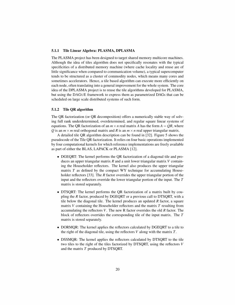
A detailed tile QR algorithm description can be found in [32]. Figure 5 shows thepseudocode of the Tile QR factorization. It relies on four basic operations implementedby four computational kernels for which reference implementations are freely availableas part of either the BLAS, LAPACK or PLASMA [12].

• DGEQRT: The kernel performs the QR factorization of a diagonal tile and pro-duces an upper triangular matrix R and a unit lower triangular matrix V contain-ing the Householder reflectors. The kernel also produces the upper triangularmatrix T as defined by the compact WY technique for accumulating House-holder reflectors [33]. The R factor overrides the upper triangular portion of theinput and the reflectors override the lower triangular portion of the input. The Tmatrix is stored separately.

• DTSQRT: The kernel performs the QR factorization of a matrix built by cou-pling the R factor, produced by DGEQRT or a previous call to DTSQRT, with atile below the diagonal tile. The kernel produces an updated R factor, a squarematrix V containing the Householder reflectors and the matrix T resulting fromaccumulating the reflectors V . The new R factor overrides the old R factor. Theblock of reflectors overrides the corresponding tile of the input matrix. The Tmatrix is stored separately.

• DORMQR: The kernel applies the reflectors calculated by DGEQRT to a tile tothe right of the diagonal tile, using the reflectors V along with the matrix T .

• DSSMQR: The kernel applies the reflectors calculated by DTSQRT to the tiletwo tiles to the right of the tiles factorized by DTSQRT, using the reflectors Vand the matrix T produced by DTSQRT.

20

1 /* Prologue, dumped "as is" in the generated file */2 extern "C" %{3 /**4 * TILE QR FACTORIZATION5 * @precisions normal z -> s d c6 */7 #include <plasma.h>8 #include <core_blas.h>9

10 #include "dague.h"11 [...] /* more includes */12 #include "dplasma/cores/cuda_stsmqr.h"13 %}14

15 /* Input variables used when creating the16 * algorithm object instance */17 descA [type = "tiled_matrix_desc_t"]18 A [type = "dague_ddesc_t *"]19 descT [type = "tiled_matrix_desc_t"]20 T [type = "dague_ddesc_t *" aligned=A]21 ib [type = "int"]22 p_work [type = "dague_memory_pool_t *"23 size = "(sizeof(PLASMA_Complex64_t)*ib*(descT.nb))"]24 p_tau [type = "dague_memory_pool_t *"25 size = "(sizeof(PLASMA_Complex64_t) *(descT.nb))"]26

27 /* Tasks descriptions follow */Figure 6: Samples from the JDF of the QR algorithm: prologue

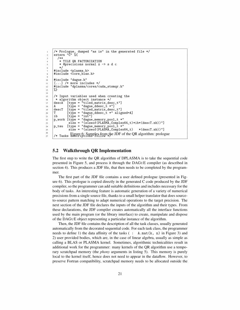
5.2 Walkthrough QR ImplementationThe first step to write the QR algorithm of DPLASMA is to take the sequential codepresented in Figure 5, and process it through the DAGUE compiler (as described insection 4). This produces a JDF file, that then needs to be completed by the program-mer.

The first part of the JDF file contains a user defined prologue (presented in Fig-ure 6). This prologue is copied directly in the generated C code produced by the JDFcompiler, so the programmer can add suitable definitions and includes necessary for thebody of tasks. An interesting feature is automatic generation of a variety of numericalprecisions from a single source file, thanks to a small helper translator that does source-to-source pattern matching to adapt numerical operations to the target precision. Thenext section of the JDF file declares the inputs of the algorithm and their types. Fromthese declarations, the JDF compiler creates automatically all the interface functionsused by the main program (or the library interface) to create, manipulate and disposeof the DAGUE object representing a particular instance of the algorithm.

Then, the JDF file contains the description of all the task classes, usually generatedautomatically from the decorated sequential code. For each task class, the programmerneeds to define 1) the data affinity of the tasks ( : A.mat(k, n) in Figure 3) and2) user provided bodies, which are, in the case of linear algebra, usually as simple ascalling a BLAS or PLASMA kernel. Sometimes, algorithmic technicalities result inadditional work for the programmer: many kernels of the QR algorithm use a tempo-rary scratchpad memory (the phony arguments in listing 5). This memory is purelylocal to the kernel itself, hence does not need to appear in the dataflow. However, topreserve Fortran compatibility, scratchpad memory needs to be allocated outside the

21

1 /* Prologue precedes, other tasks */2

3 ztsmqr(k,m,n)4 [...] /* Execution space (autogenerated) */5

6 /* Variable names translation table (autogenerated) */7 /* J == A(k,n) */8 [...] /* more translations */9

10 /* dependencies (autogenerated)11 RW J <- (m==k+1) ? E zunmqr(m-1,n) : J ztsmqr(k,m-1,n)12 -> (m==descA.mt-1) ? J ztsmqr_out_A(k,n) : J ztsmqr(k,m+1,n)13 [...] /* more dependencies */14

15 /* Task affinity with data (edited by programmer) */16 : A(m, n)17

18 BODY /* edited by programmer */19 /* computing tight tile dimensions20 * (tiles on matrix edges contain padding) */21 int tempnn = (n==descA.nt-1) ? descA.n-n*descA.nb : descA.nb;22 int tempmm = (m==descA.mt-1) ? descA.m-m*descA.mb : descA.mb;23 int ldak = BLKLDD( descA, k );24 int ldam = BLKLDD( descA, m );25

26 /* Obtain a scratchpad allocation */27 void* p_elem_A = dague_private_memory_pop( p_work );28 /* Call to the actual kernel */29 CODELET_ztsmqr(PlasmaLeft, PlasmaConjTrans, descA.mb,30 tempnn, tempmm, tempnn, descA.nb, ib,31 J /* A(k,n) */, ldak,32 K /* A(m,n) */, ldam,33 L /* A(m,k) */, ldam,34 M /* T(m,k) */, descT.mb,35 p_elem_A, ldwork );36 /* Release the scratchpad allocation */37 dague_private_memory_push( p_work, p_elem_A );38 END

Figure 7: Samples from the JDF of the QR algorithm: task body

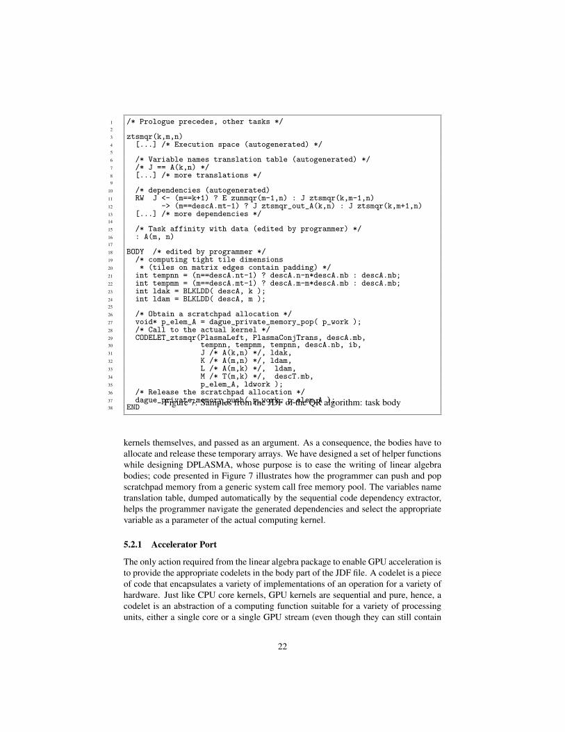
kernels themselves, and passed as an argument. As a consequence, the bodies have toallocate and release these temporary arrays. We have designed a set of helper functionswhile designing DPLASMA, whose purpose is to ease the writing of linear algebrabodies; code presented in Figure 7 illustrates how the programmer can push and popscratchpad memory from a generic system call free memory pool. The variables nametranslation table, dumped automatically by the sequential code dependency extractor,helps the programmer navigate the generated dependencies and select the appropriatevariable as a parameter of the actual computing kernel.

5.2.1 Accelerator Port

The only action required from the linear algebra package to enable GPU acceleration isto provide the appropriate codelets in the body part of the JDF file. A codelet is a pieceof code that encapsulates a variety of implementations of an operation for a variety ofhardware. Just like CPU core kernels, GPU kernels are sequential and pure, hence, acodelet is an abstraction of a computing function suitable for a variety of processingunits, either a single core or a single GPU stream (even though they can still contain

22

1 dague_object_t* dplasma_sgeqrf_New( tiled_matrix_desc_t *A,2 tiled_matrix_desc_t *T )3 {4 dague_sgeqrf_object_t* d = dague_sgeqrf_new(*A, (dague_ddesc_t*)A,5 *T, (dague_ddesc_t*)T,6 ib, NULL, NULL);7

8 d->p_tau = malloc(sizeof(dague_memory_pool_t));9 dague_private_memory_init(d->p_tau, T->nb * sizeof(float));

10 [...] /* similar code for p_work scratchpad */11

12 /* Datatypes declarations, from MPI datatypes */13 dplasma_add2arena_tile(d->arenas[DAGUE_sgeqrf_DEFAULT_ARENA],14 A->mb*A->nb*sizeof(float),15 DAGUE_ARENA_ALIGNMENT_SSE,16 MPI_FLOAT, A->mb);17 /* Lower triangular part of tile without diagonal */18 dplasma_add2arena_lower(d->arenas[DAGUE_sgeqrf_LOWER_TILE_ARENA],19 A->mb*A->nb*sizeof(float),20 DAGUE_ARENA_ALIGNMENT_SSE,21 MPI_FLOAT, A->mb, 0);22 [...] /* similarly, U upper triangle and T (IB*MB rectangle)*/23

24 return (dague_object_t*)d;25 }

Figure 8: User provided wrapper around the DAGUE generated QR factorization func-tion

some internal parallelism, such as vector SIMD instructions). Practically, that meansthat the application developer is in charge of providing multiple versions of the com-puting bodies. The relevant codelets, optimized for the current hardware, are loadedautomatically during the algorithm initialization (one for the GPU hardware, one for theCPU cores, etc). Today, the DAGUE runtime supports only CUDA and CPU codelets,but the infrastructure can easily accommodate other accelerator types (MIC, OpenCL,FPGAs, Cell, ...). If a task features multiple codelets, the runtime scheduler choosesdynamically (during the invocation of the automatically generated scheduling hookCODELET kernelname) between all these versions, in order to execute the operationon the most relevant hardware. Because multiple versions of the same codelet kernelcan be in use at the same time, the workload of this type of operations, on differentinput data, can be distributed on both CPU cores and GPUs simultaneously.

In the case of the QR factorization, we selected to add a GPU version of theSTSMQR kernel, which is the matrix-matrix multiplication kernel used to update theremainder of the matrix, after a particular panel has been factorized (hence representing80% or more of the overall compute time). We have extended a handmade GPU ker-nel [34], originally obtained from MAGMA [12]. This kernel is provided in a separatesource file, and is developed separately as a regular CUDA function. Should future ver-sions of CuBLAS enable running concurrent GPU kernels on several hardware streams,these vendor functions could be used directly.

5.2.2 Wrapper

As previously stated, scratchpad memory needs to be allocated outside of the bodies.Similarly, because we wanted the JDF format to be oblivious of the transport technol-

23

1 int main(int argc, char **argv)2 {3 dague_context_t *dague;4 two_dim_block_cyclic_t ddescA;5 two_dim_block_cyclic_t ddescT;6 dague_object_t* zgeqrf_object;7

8 MPI_Init(&argc, &argv);9 [...]

10

11 dague = dague_init(NBCORES, &argc, &argv);12 dague_set_scheduler(dague, &dague_sched_LHQ);13

14 /* Matrix allocation and random filling */15 two_dim_block_cyclic_init(&ddescA, matrix_ComplexDouble, [...]);16 ddescA.mat = dague_data_allocate([...]);17 dplasma_zplrnt(dague, &ddescA, 3872);18 dplasma_zlaset(dague, PlasmaUpperLower, 0., 0., &ddescT);19 [...] /* Same for other matrices */20

21 zgeqrf_object = dplasma_zgeqrf_New(&ddescA, &ddescT);22 dague_enqueue(dague, zgeqrf_object);23

24 /* Computation happens here */25 dague_progress(dague);26

27 dplasma_zgeqrf_Destruct(zgeqrf_object);28

29 [...]30

31 dague_data_free(ddescA.mat);32 dague_ddesc_destroy((dague_ddesc_t*)&ddescA);33 [...]34

35 dague_fini(&dague);36 MPI_Finalize();37

38 return 0;39 }

Figure 9: Skeleton of a DAGUE main program driving the QR factorization

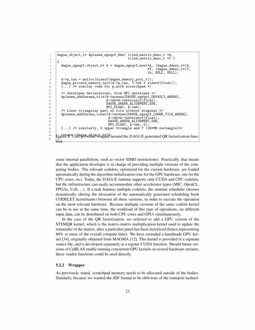
ogy, datatypes, which are inherently dependent on the description used in the messagepassing system, need to be declared outside the generated code. In order for the gen-erated library to be more convenient to use for end-users, we consider it good practiceto provide a wrapper around the generated code that takes care of allocating and defin-ing these required elements. In the case of linear algebra, we provide a variety ofhelper functions to allocate scratchpads (line 11 in listing 8), and to create most use-ful datatypes (like triangular matrices (lines 15, 21 in the listing), like band matrices,square or rectangular matrices, etc. Again, the framework provided tool can create allfloating point precisions from a single source.

5.2.3 Main Program

A skeleton program that initializes and schedules a QR factorization using theDAGUE framework is presented in Figure 9. Since DAGUE uses MPI as an underlay-ing communication mechanism, the test program is an MPI program. It thus needs toinitialize and finalize MPI (lines 8 and 33) and the programmer is free to use any MPI

24

functionality, around DAGUE calls (line 9, where arguments should also be parsed). Asubset of the DAGUE calls are to be considered as collective operations from an MPIperspective: all MPI processes must call them in the same order, with a communicationscheme that allows these operations to match. These operations are the initializationfunction (dague init), the progress function (dague progress) and the finalizationfunction (dague fini). dague init will create a specified number of threads on thelocal process, plus the communication thread. Threads are bound on separate coreswhen possible. Once the DAGUE system is initialized on all MPI processes, eachmust choose a local scheduler. DAGUE provides four scheduling heuristics, but theone preferred is the Local Hierarchical Scheduler, developed specifically for DAGUEon NUMA many-core heterogeneous machines. The function dague set scheduler

of line 12 sets this scheduler.The next step consists of creating a data distribution descriptor. This code holds two

data distribution descriptors: ddescA and ddescT. DAGUE provides three built-in datadistributions for tiled matrices: an arbitrary index based distribution; a symmetric twodimensional block cyclic distribution, and a two dimensional block cyclic distribution.In the case of QR, the latter is used to describe the input matrix A to be factorized, andthe workspace array T. Once the data distribution is created, the local memory to storethis data should be allocated in the fields mat of the descriptor. To enable DAGUE topin memory, and allow for direct DMA transfers (to and from the GPUs or some highperformance networks), the helper function dague data allocate of line 15 is used.The workspace array T should be described and allocated in a similar way on line 16.

Then, this test program uses DPLASMA functions to initialize the matrix A withrandom values (line 18), and the workspace array T with 0 (line 19). These functionsare coded in DAGUE: they create a DAG representation of a map operation that willinitialize each tile in parallel with the desired values, making the engine progress onthese DAGs.

Once the data is initialized, a zgeqrf DAGUE object is created with the wrapperthat was described above. This object holds the symbolic representation of the localDAG, initialized with the desired parameters, and bound to the allocated and describeddata. It is (locally) enqueued in the DAGUE engine on line 22.

To compute the QR operation described by this object, all MPI processes call todague progress on line 24. This enables all threads created on line 8 to work on theQR operation enqueued before in collaboration with all the other MPI processes. Thiscall returns when all enqueued objects are completed, thus when the factorization isdone. At this point, the zgeqrd DAGUE Object is consumed, and can be freed by theprogrammer at line 26. The result of the factorization should be used on line 28, beforethe data is freed (line 30), and the descriptors destroyed (line 31). Line 32 shouldhold similar code to free the data and destroy the descriptor of T. Then, the DAGUEengine can release all resources (line 34) before MPI is finalized and the applicationterminates.

5.2.4 SPMD library interface

It is possible for the library to encapsulate all dataflow related calls inside a regu-lar (ScaLAPACK like) interface function. This function creates an algorithm instance,

25

1 int dplasma_sgeqrf( dague_context_t *dague, tiled_matrix_desc_t *A,2 tiled_matrix_desc_t *T )3 {4 dague_object_t *dague_sgeqrf = dplasma_sgeqrf_New(A, T);5

6 dague_enqueue(dague, dague_sgeqrf);7 dplasma_progress(dague);8

9 dplasma_sgeqrf_Destruct(dague_sgeqrf);10 return 0;11 }

Figure 10: DPLASMA SPMD interface for the DAGUE generated QR factorizationfunction

enqueues it in the dataflow runtime and enables progress (lines 6, 8, 9 in listing 10).From the main program point of view, the code is similar to a SPMD call to a parallelBLAS function; the main program does not need to consider the fact that dataflow isused within the linear algebra library. While this approach can simplify the porting oflegacy applications, it prevents the program from composing DAG based algorithms.If the main program takes full control of the algorithm objects, it can enqueue multi-ple algorithms, and then progress all of them simultaneously, enabling optimal overlapbetween separate algorithms (such as a factorization and the associated solve); if itsimply calls the SPMD interface, it still benefits from complete parallelism within in-dividual functions, but it falls back to a synchronous SPMD model between differentalgorithms.

5.3 Correctness and Performance Analysis ToolsThe first correctness tool of the DAGUE framework sits within the code generator tool,which converts the JDF representation into C functions. A number of conditions on thedependencies and execution spaces are checked during this stage, and can detect manyinstances of mismatching dependencies (where the input of task A comes from taskB, but task B has no outputs to task A). Similarly, conditions that are not satisfiableaccording to the execution space raise warnings, as is the case for pure input data(operations that read the input matrix directly, not as an output of another task) that donot respect the task-data affinity. There warnings help the programmer detect the mostcommon errors when writing the JDF.

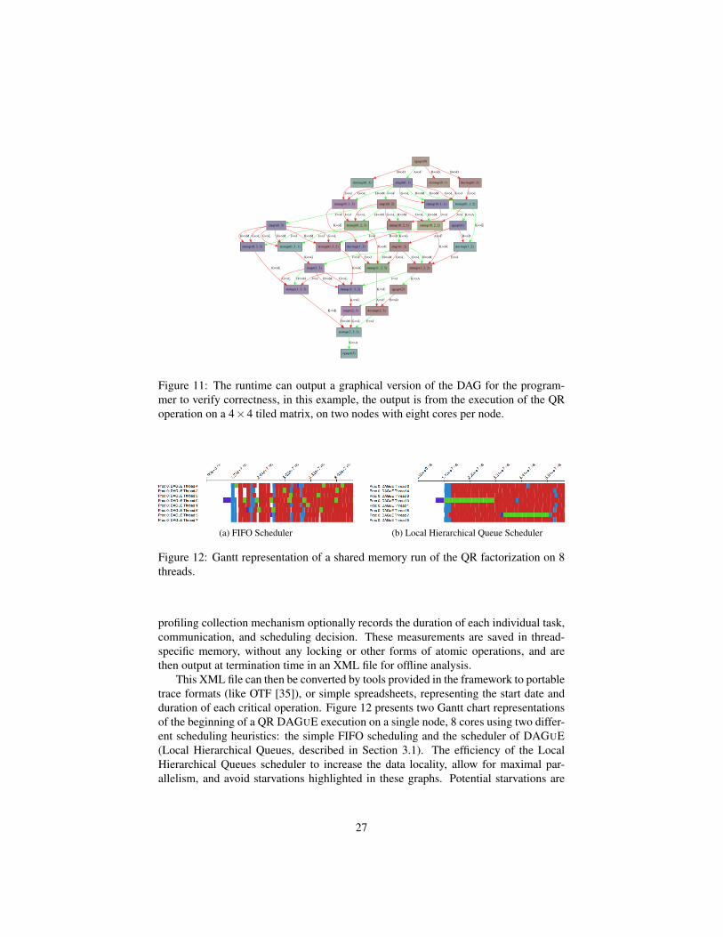
At runtime, algorithm programmers can generate the complete unrolled DAG, foroffline analysis purposes. The DAGUE engine can output a representation of the DAG,as it is executed, in the dot input format of the GraphViz graph plotting tool. The pro-grammer can use the resulting graphic representation (see Figure 11) to analyze whichkernel ran on what resource, and which dependence released which tasks into theirready state. Using such information has proven critical when debugging the JDF repre-sentation (for an advanced user who wants to write her own JDF directly without usingthe DAGUE compiler), or to understand contentions and improve the data distributionand the priorities assigned to tasks.

The DAGUE framework also features performance analysis tools to help program-mers fine-tune the performance of their application. At the heart of these tools, the

26

zgeqrt(0)

dormqr(0, 1)

B=>D

dormqr(0, 2)

B=>D

dormqr(0, 3)

B=>D

ztsqrt(0, 1)

A=>F

ztsmqr(0, 1, 1)

E=>J

ztsmqr(0, 1, 2)

E=>J

ztsmqr(0, 1, 3)

E=>J

ztsmqr(0, 2, 3)

J=>J

dormqr(1, 3)

K=>E

ztsmqr(1, 2, 3)

K=>Kztsmqr(0, 3, 3)

J=>J

ztsmqr(0, 2, 1)

J=>J

zgeqrt(1)

K=>A

ztsqrt(1, 2)

K=>G

ztsmqr(0, 3, 1)

J=>J

G=>L H=>M G=>L H=>M

ztsqrt(0, 2)

F=>F G=>LH=>M

G=>L H=>M G=>L H=>M

ztsmqr(0, 2, 2)

G=>L H=>M

ztsqrt(0, 3)

F=>F

E=>J

dormqr(2, 3)

K=>Eztsmqr(1, 3, 3)

J=>J

J=>J

dormqr(1, 2)

K=>E

ztsmqr(1, 2, 2)

K=>Kztsmqr(0, 3, 2)

J=>J B=>D A=>F B=>D

G=>LH=>M G=>L H=>M

ztsqrt(1, 3)

F=>F E=>J

zgeqrt(2)

K=>A

ztsmqr(1, 3, 2)

J=>J

ztsmqr(2, 3, 3)

E=>J

B=>D

ztsqrt(2, 3)

A=>F

G=>L H=>M G=>LH=>MG=>LH=>M

K=>G

K=>KK=>K

K=>K

K=>G

G=>L H=>M G=>LH=>M

zgeqrt(3)

K=>A

G=>LH=>M

Figure 11: The runtime can output a graphical version of the DAG for the program-mer to verify correctness, in this example, the output is from the execution of the QRoperation on a 4×4 tiled matrix, on two nodes with eight cores per node.

(a) FIFO Scheduler (b) Local Hierarchical Queue Scheduler

Figure 12: Gantt representation of a shared memory run of the QR factorization on 8threads.

profiling collection mechanism optionally records the duration of each individual task,communication, and scheduling decision. These measurements are saved in thread-specific memory, without any locking or other forms of atomic operations, and arethen output at termination time in an XML file for offline analysis.

This XML file can then be converted by tools provided in the framework to portabletrace formats (like OTF [35]), or simple spreadsheets, representing the start date andduration of each critical operation. Figure 12 presents two Gantt chart representationsof the beginning of a QR DAGUE execution on a single node, 8 cores using two differ-ent scheduling heuristics: the simple FIFO scheduling and the scheduler of DAGUE(Local Hierarchical Queues, described in Section 3.1). The efficiency of the LocalHierarchical Queues scheduler to increase the data locality, allow for maximal par-allelism, and avoid starvations highlighted in these graphs. Potential starvations are

27

easily spotted, as they appear as large stripes where multiple threads do not executeany kernel. Similar charts can be generated for distributed runs (not presented here),with a clear depiction of the underlying communications in the MPI thread, annotatedby the data they carry and tasks they connect. Using these results, a programmer canassess the efficiency, on real runs, of the proposed data distribution, task affinity, andpriority. Data distribution and task affinity will both influence the amount and dura-tion of communications, as well as the amount of starvation, while Priority will mostlyinfluence the amount of starvation.

In the case of the QR factorization, these profiling outputs have been used to eval-uate the priority hints given to tasks, used by the scheduler when ordering tasks (referto Section 3.1). The folklore knowledge about scheduling DAG of dense factorizationsis that the priorities should always favor the tasks that are closer to the critical path.We have implemented such a strategy, and discovered that it is easily outperformed bya completely dynamic scheduling that does not respect any priorities. There is indeeda fine balance between following the absolute priorities along the critical path, whichenables maximum parallelism, and favoring cache reuse even if it progresses a branchthat is far from the critical path. We have found a set of beneficial priority rules (whichare symbolic expressions similar to the dependencies) which favor progressing itera-tions along the ”k” direction first, but favoring only a couple iterations of the criticalpath over update kernels.

6 Performance EvaluationThe performance of the DAGUE runtime have been extensively studied in related pub-lications [36, 37, 4, 34]. The goal here is to illustrate the performance results that can beachieved by the porting of linear algebra code to the DAGUE framework. Therefore,we present a summary of these result, to demonstrate that the tool chain achieves itsmain goals of overall performance, performance portability, and capability to processdifferent non-trivial algorithms.

The experiments we summarize here have been conducted on three different plat-forms. The Griffon platform is one of the clusters of Grid’5000 [38]. We used 81 dualsocket Intel Xeon L5420 quad core processors at 2.5 GHz to gather 648 cores. Eachnode has 16GB of memory, and is interconnected to the others by a 20 Gbs Infinibandnetwork. Linux 2.6.24 (Debian Sid) is deployed on these nodes. The Kraken system ofthe University of Tennessee and National Institute for Computational Science (NICS)is hosted at the Oak Ridge National Laboratory. It is a Cray XT5 with 8,256 computenodes connected on a 3D torus with SeaStar. Each node has a dual six-core AMDOpteron cadenced at 2.6GHz. We used up to 3,072 cores in the experiments we presenthere. All nodes have 16GB of memory, and run the Cray Linux Environment (CLE)2.2.

The benchmark consists of three popular dense matrix factorizations: Cholesky, LUand QR. The Cholesky factorization solves the problem Ax = b, where A is symmetricand positive definite. It computes the real lower triangular matrix with positive diago-nal elements L such that A = LLT . The QR factorization has been presented in previoussections, to explain the functionality and behavior of DAGUE. It offers a numerically

28

0

1

2

3

4

5

6

7

13k

26k

40k

53k

67k

80k

94k

107k120k

130k

TF

lop

/s

Matrix size (N)

DPOTRF performance problem scaling648 cores (Myrinet 10G)

Theoretical peakPractical peak (GEMM)DAGuEDSBPScaLAPACK

(a) Cholesky Factorization

0

1

2

3

4

5

6

7

13k

26k

40k

53k

67k

80k

94k

107k120k

130k

TF

lop

/sMatrix size (N)

DGETRF performance problem scaling648 cores (Myrinet 10G)

Theoretical peakPractical peak (GEMM)DAGuEHPLScaLAPACK

(b) LU Factorization

0

1

2

3

4

5

6

7

13k

26k

40k

53k

67k

80k

94k

107k120k

130k

TF

lop

/s

Matrix size (N)

DGEQRF performance problem scaling648 cores (Myrinet 10G)

Theoretical peakPractical peak (GEMM)DAGuEScaLAPACK

(c) QR Factorization

Figure 13: Performance comparison on the Griffon platform with 648 cores.

stable way of solving full rank underdetermined, overdetermined, and regular squarelinear systems of equations. It computes Q and R such that A = QR, Q is a real orthog-onal matrix, and R is a real upper triangular matrix. The LU factorization with partialpivoting of a real matrix A has the form PA = LU where L is a real unit lower triangularmatrix, U is a real upper triangular matrix, and P is a permutation matrix.

All three of these operations are implemented in the ScaLAPACK numerical li-brary [39]. In addition, some of these factorizations have more optimized versions,we used the state of the art version for each of the existing factorizations to measureagainst. The Cholesky factorization has been implemented in a more optimized wayin the DSBP software [16], using static scheduling of tasks, and a specific, more ef-ficient, data distribution. The LU factorization with partial pivoting is also solved bythe well known High Performance LINPACK benchmark (HPL) [40], used to mea-sure the performance of high performance computers. We have distributed the initialdata following a classical 2D-block cyclic distribution used by ScaLAPACK, and usedthe DAGUE runtime engine to schedule the operations on the distributed data. Thekernels consist of the BLAS operations referenced by the sequential codes, and theirimplementation was the most efficient available on each of the machine.

Figure 13 presents the performance measured for DAGUE and ScaLAPACK, andwhen applicable DSBP and HPL, as a function of the problem size. 648 cores on 81multi-core nodes have been used for the distributed run, and the data was distributedaccording to a 9×9 2D block-cyclic grid for DAGUE. A similar distribution was usedfor ScaLAPACK, and the other benchmarks when appropriate, and the block size wastuned to provide the best performance on each setup. As the figures illustrate, on allbenchmarks, and for all problem sizes, the DAGUE framework was able to outperformScaLAPACK, and perform as well as the state of the art, hand-tuned codes for specificproblems. The DAGUE solution goes from the sequential code to the parallel runcompletely automatically, but is still able to outperform DSBP, and competes with theHPL implementation on this machine.

Figure 14a presents the performance of the DAGUE Cholesky algorithm on a GPUcluster, featuring 12 Fermi C2070 accelerators (one per node). Without GPU acceler-

29

0

1

2

3

4

5

6

7

8

9

10

20k 30k 40k 50k 60k 70k 80k 90k 100k110k

120k

Pe

rfo

rman

ce (

TF

lop

/s)

Matrix Size

SPOTRF performance problem scaling12 GPU nodes (Infiniband 20G)

Practical peak (GEMM)C2070 + 8 cores per node8 cores per node

(a) Efficiency at 12 nodes

0

1

2

3

4

5

6

7

8

9

10

1;5

4k

2;7

6k

4;1

08k

8;1

52k

12;1

76k

Pe

rfo

rman

ce (

TF

lop

/s)

Number of Nodes;Matrix Size (N)

SPOTRF performance weak scaling12 GPU nodes (Infiniband 20G)

Practical peak (GEMM)C2070 + 8 cores per node8 cores per node

(b) Scalability

Figure 14: Performance of DAGUE Cholesky on the Dancer GPU accelerated cluster.

0

5

10

15

20

25

30

108 432

768 1200

3072

Perf

orm

an

ce

(T

Flo

p/s

)

Number of cores

DGEQRF performance weak scalingCray XT5

Practical peak (GEMM)DAGuElibSCI Scalapack

Figure 15: Scalability on the Kraken platform.

ators, the DAGUE runtime extracts the entire available performance; asymptotic per-formance matches the performance of the GEMM kernel on this processor, which is anupper bound to the effective peak performance. When using one GPU accelerator pernode, the total efficiency reaches as much as 73% of the GEMM peak, which is a 54%efficiency of the theoretical peak (typical GPU efficiency is lower than CPU efficiency;the HPL benchmark on the TianHe-1A GPU system reaches a similar 51% efficiency,which compares with 78% on the CPU based Kraken machine). Scalability is a con-cern with GPU accelerators, as they provoke a massive imbalance between computingpower and network capacity. Figure 14b presents the Cholesky factorization weak scal-ability (number of nodes vary, problem size is growing accordingly to keep memoryload per node constant) on the GPU enabled machine. The figure outlines the perfectweak scalability up to 12 GPU nodes.

Last, Figure 15 compares the performance of the DAGUE implementation of thesethree operations with the libSCI implementation, specifically tuned by Cray for thismachine. The value represented is the relative time overhead of DAGUE comparedto libSCI for different matrix sizes and the number of nodes on the QR factorization(similar weak scaling as in the previous experiment, N=454000 on 3072 cores). On this

30

machine, the DAGUE runtime can effectively use only 11 of 12 cores per node for com-pute tasks; due to kernel scheduler parameters (long, non-preemptive time quantum),the MPI thread must be exclusively pinned to a physical core to avoid massive anddetrimental message jitter. Even considering that limitation, which is only technicaland could be overcome by a native port of the runtime to the Portals messaging libraryinstead of MPI, the DAGUE implementation competes favorably with the extremelyefficient libSCI QR factorization. The DAGUE approach demonstrates an excellentscalability, up to a massive number of nodes, thanks to the distributed evaluation ofthe DAG not requiring centralized control nor complete unrolling of the DAG on eachnode.

On different machines, the DAGUE compiler coupled with the DAGUE runtimesignificantly outperformed standard algorithms, and competed closely, usually favor-ably, with state-of-the-art optimized versions of similar algorithms, without any furthertuning process involved when porting the code between radically different platformtypes. Another significant fact to be highlighted is the sizes of the problem whereDAGUE achieves peak performance. In all graphs in Figure 13 one can notice thatwhile Scalapack asymptotically reaches peak performance, for some of the algorithmsDAGUE achieves the same level of performance on data 4 times smaller (in the caseof Cholesky, Scalapack achieves 3TFlop/s on Griffon when N = 130k, while DAGUEreaches the same level for N = 44k).

7 ConclusionAlthough hardware architectural paradigm shifts are threatening the scientific pro-ductivity of dense linear algebra codes, we have demonstrated that slightly changingthe execution paradigm, and using a dataflow representation extracted from a dec-orated sequential code, dense matrix factorization can reach excellent performance.The DPLASMA package aims at providing the same functionalities as the ScaLA-PACK legacy package, but using a more modern approach, based on tile algorithmand dataflow representation, that enables better cache reuse and asynchrony, which areparamount features to perform on multicore nodes. Furthermore, the DAG dataflowrepresentation enables the algorithm to adapt easily to a variety of differing and hetero-geneous hardware, without involving a major code refactoring for each target platform.We describe how the DPLASMA project uses the DAGUE framework to convert adecorated sequential code (which can be executed efficiently on multicore machines,but not on distributed memory systems), into a concise DAG dataflow representation.This representation is then altered by the programmer to add data distribution and taskaffinity on distributed memory. The resulting intermediate format is then compiledinto a series of runtime hooks incorporating a DAG scheduler that automatically or-chestrates the resolution of remote dependencies, orchestrates the execution to favorcache locality and other scheduling heuristics, and accounts for the presence of hetero-geneous resources such as GPU accelerators. This description gives insight to linearalgebra programmers as to the methods, challenges and solutions involved in portingtheir code to a dataflow representation. The performance analysis section demonstratesthe vast superiority of the DAG based code over legacy programming paradigms on

31

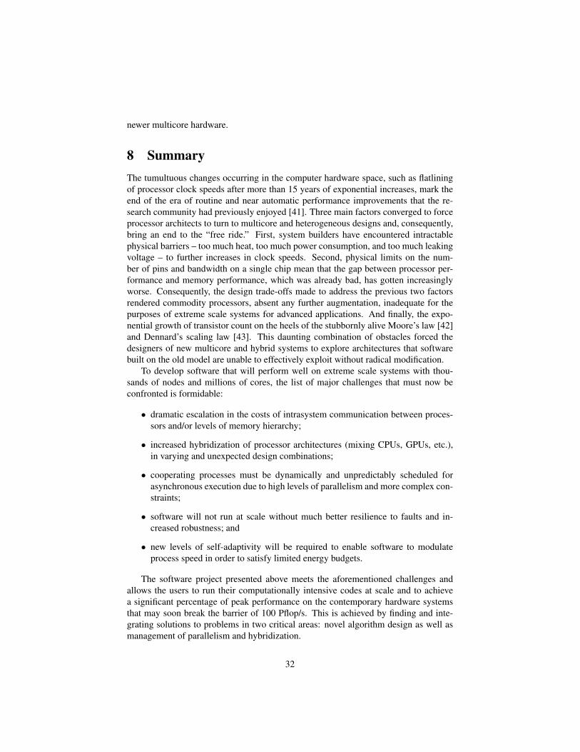
newer multicore hardware.

8 SummaryThe tumultuous changes occurring in the computer hardware space, such as flatliningof processor clock speeds after more than 15 years of exponential increases, mark theend of the era of routine and near automatic performance improvements that the re-search community had previously enjoyed [41]. Three main factors converged to forceprocessor architects to turn to multicore and heterogeneous designs and, consequently,bring an end to the “free ride.” First, system builders have encountered intractablephysical barriers – too much heat, too much power consumption, and too much leakingvoltage – to further increases in clock speeds. Second, physical limits on the num-ber of pins and bandwidth on a single chip mean that the gap between processor per-formance and memory performance, which was already bad, has gotten increasinglyworse. Consequently, the design trade-offs made to address the previous two factorsrendered commodity processors, absent any further augmentation, inadequate for thepurposes of extreme scale systems for advanced applications. And finally, the expo-nential growth of transistor count on the heels of the stubbornly alive Moore’s law [42]and Dennard’s scaling law [43]. This daunting combination of obstacles forced thedesigners of new multicore and hybrid systems to explore architectures that softwarebuilt on the old model are unable to effectively exploit without radical modification.

To develop software that will perform well on extreme scale systems with thou-sands of nodes and millions of cores, the list of major challenges that must now beconfronted is formidable:

• dramatic escalation in the costs of intrasystem communication between proces-sors and/or levels of memory hierarchy;

• increased hybridization of processor architectures (mixing CPUs, GPUs, etc.),in varying and unexpected design combinations;

• cooperating processes must be dynamically and unpredictably scheduled forasynchronous execution due to high levels of parallelism and more complex con-straints;

• software will not run at scale without much better resilience to faults and in-creased robustness; and

• new levels of self-adaptivity will be required to enable software to modulateprocess speed in order to satisfy limited energy budgets.

The software project presented above meets the aforementioned challenges andallows the users to run their computationally intensive codes at scale and to achievea significant percentage of peak performance on the contemporary hardware systemsthat may soon break the barrier of 100 Pflop/s. This is achieved by finding and inte-grating solutions to problems in two critical areas: novel algorithm design as well asmanagement of parallelism and hybridization.

32

References[1] P. Kogge, K. Bergman, S. Borkar, D. Campbell, W. Carlson, W. Dally, M. Den-

neau, P. Franzon, W. Harrod, K. Hill, J. Hiller, S. Karp, S. Keckler, D. Klein,R. Lucas, M. Richards, A. Scarpelli, S. Scott, A. Snavely, T. Sterling, R. S.Williams, and K. Yelick, “Exascale computing study: Technology challenges inachieving exascale systems,” Tech. Rep. TR-2008-13, Department of ComputerScience and Engineering, University of Notre Dame, September 28 2008.

[2] National Research Council Committee on the Potential Impact of High-End Com-puting on Illustrative Fields of Science and Engineering, The Potential Impact ofHigh-End Capability Computing on Four Illustrative Fields of Science and Engi-neering. Washington, DC: National Academies Press, 2008.

[3] University of Tennessee, PLASMA Users’ Guide, Parallel Linear Algebra Soft-ware for Multicore Architectures, Version 2.2, November 2009.

[4] G. Bosilca, A. Bouteiller, A. Danalis, T. Herault, P. Lemarinier,and J. J. Dongarra, “DAGuE: A generic distributed DAG engine forhigh performance computing,” Parallel Computing, 2011. to appear,http://dx.doi.org/10.1016/j.parco.2011.10.003.

[5] E. G. Coffman, Jr. and P. J. Denning, Operating Systems Theory. Prentice HallProfessional Technical Reference, 1973.

[6] A. J. Bernstein, “Analysis of programs for parallel processing,” Electronic Com-puters, IEEE Transactions on, vol. EC-15, pp. 757 –763, Oct. 1966.

[7] J. A. Sharp, ed., Data flow computing: theory and practice. Ablex PublishingCorp, 1992.

[8] J. Yu and R. Buyya, “A taxonomy of workflow management systems for gridcomputing,” tech. rep., Journal of Grid Computing, 2005.

[9] O. Delannoy, N. Emad, and S. Petiton, “Workflow global computing with YML,”in 7th IEEE/ACM International Conference on Grid Computing, September 2006.

[10] A. Buttari, J. J. Dongarra, J. Kurzak, J. Langou, P. Luszczek, and S. Tomov, “Theimpact of multicore on math software,” in Applied Parallel Computing. State ofthe Art in Scientific Computing, 8th International Workshop, PARA, vol. 4699 ofLecture Notes in Computer Science, pp. 1–10, Springer, 2006.

[11] E. Chan, F. G. Van Zee, P. Bientinesi, E. S. Quintana-Ortı, G. Quintana-Ortı, andR. van de Geijn, “Supermatrix: a multithreaded runtime scheduling system foralgorithms-by-blocks,” in PPoPP ’08: Proceedings of the 13th ACM SIGPLANSymposium on Principles and practice of parallel programming, pp. 123–132,ACM, 2008.

33

[12] E. Agullo, J. Demmel, J. J. Dongarra, B. Hadri, J. Kurzak, J. Langou, H. Ltaief,P. Luszczek, and S. Tomov, “Numerical linear algebra on emerging architectures:The PLASMA and MAGMA projects,” Journal of Physics: Conference Series,vol. 180, 2009.

[13] R. Dolbeau, S. Bihan, and F. Bodin, “HMPP: A hybrid multi-core parallel pro-gramming environment,” in Workshop on General Purpose Processing on Graph-ics Processing Units (GPGPU 2007), 2007.

[14] C. Augonnet, S. Thibault, R. Namyst, and P.-A. Wacrenier, “StarPU: a unifiedplatform for task scheduling on heterogeneous multicore architectures,” Concur-rency and Computation: Practice and Experience, vol. 23, no. 2, pp. 187–198,2011.

[15] P. Husbands and K. A. Yelick, “Multi-threading and one-sided communicationin parallel LU factorization,” in Proceedings of the ACM/IEEE Conference onHigh Performance Networking and Computing, SC 2007, November 10-16, 2007,Reno, Nevada, USA (B. Verastegui, ed.), ACM Press, 2007.

[16] F. G. Gustavson, L. Karlsson, and B. Kagstrom, “Distributed SBP Cholesky fac-torization algorithms with near-optimal scheduling,” ACM Trans. Math. Softw.,vol. 36, no. 2, pp. 1–25, 2009.

[17] J. Perez, R. Badia, and J. Labarta, “A dependency-aware task-based programmingenvironment for multi-core architectures,” in Cluster Computing, 2008 IEEE In-ternational Conference on, pp. 142 –151, 29 2008-oct. 1 2008.

[18] F. Song, A. YarKhan, and J. J. Dongarra, “Dynamic task scheduling for linear al-gebra algorithms on distributed-memory multicore systems,” in SC ’09: Proceed-ings of the Conference on High Performance Computing Networking, Storage andAnalysis, (New York, NY, USA), pp. 1–11, ACM, 2009.

[19] M. Cosnard and E. Jeannot, “Automatic Parallelization Techniques Based onCompact DAG Extraction and Symbolic Scheduling,” Parallel Processing Let-ters, vol. 11, pp. 151–168, 2001.

[20] M. Cosnard, E. Jeannot, and T. Yang, “Compact dag representation and itssymbolic scheduling,” Journal of Parallel and Distributed Computing, vol. 64,pp. 921–935, August 2004.

[21] E. Jeannot, “Automatic multithreaded parallel program generation for messagepassing multiprocessors using parameterized task graphs,” in International Con-ference ’Parallel Computing 2001’ (ParCo2001), September 2001.

[22] A. Haidar, H. Ltaief, A. YarKhan, and J. J. Dongarra, “Analysis of dynamicallyscheduled tile algorithms for dense linear algebra on multicore architectures,”Concurrency and Computation: Practice and Experience, pp. n/a–n/a, 2011.

[23] AMD, “Amd64 architecture programmer’s manual volume 2: System program-ming,” tech. rep., AMD64 Technology, 2011.

34

[24] W. Pugh, “The omega test: a fast and practical integer programming algorithmfor depend ence analysis,” in Supercomputing ’91: Proceedings of the 1991ACM/IEEE conference on Supercomputing, (New York, NY, USA), pp. 4–13,1991.

[25] R. Harrington, “Origin and development of the method of moments for field com-putation,” IEEE Antennas and Propagation Magazine, June 1990.

[26] J. J. H. Wang, Generalized Moment Methods in Electromagnetics. New York:John Wiley & Sons, 1991.

[27] J. L. Hess, “Panel methods in computational fluid dynamics,” Annual Reviews ofFluid Mechanics, vol. 22, pp. 255–274, 1990.

[28] L. Hess and M. O. Smith, “Calculation of potential flows about arbitrary bod-ies,” in Progress in Aeronautical Sciences (D. Kuchemann, ed.), vol. 8, PergamonPress, 1967.

[29] A. Edelman, “Large dense numerical linear algebra in 1993: the parallel comput-ing influence,” International Journal of High Performance Computing Applica-tions, vol. 7, no. 2, pp. 113–128, 1993.

[30] R. F. Barrett, T. H. F. Chan, E. F. D’Azevedo, E. F. Jaeger, K. Wong, and R. Y.Wong, “Complex version of high performance computing LINPACK benchmark(HPL),” Concurrency and Computation: Practice and Experience, vol. 22, no. 5,pp. 573–587, 2010.

[31] G. W. Stewart, “The decompositional approach to matrix computation,” Comput-ing in Science & Engineering, vol. 2, pp. 50–59, Jan/Feb 2000. ISSN: 1521-9615;DOI 10.1109/5992.814658.

[32] A. Buttari, J. Langou, J. Kurzak, and J. J. Dongarra, “Parallel tiled QR factor-ization for multicore architectures,” tech. rep., Innovative Computing Laboratory,University of Tennessee, 2007.

[33] R. Schreiber and C. van Loan, “A storage-efficient WY representation for prod-ucts of Householder transformations,” J. Sci. Stat. Comput., vol. 10, pp. 53–57,1991.

[34] G. Bosilca, A. Bouteiller, T. Herault, P. Lemarinier, N. Saengpatsa, S. Tomov,and J. J. Dongarra, “Performance portability of a GPU enabled factorization withthe DAGuE framework,” in Proceedings of the IEEE Cluster 2011 Conference(PPAC Workshop), pp. 395–402, IEEE, September 2011.

[35] A. D. Malony and W. E. Nagel, “The open trace format (OTF) and open tracingfor HPC,” in Proceedings of the 2006 ACM/IEEE conference on Supercomputing,SC ’06, (New York, NY, USA), ACM, 2006.

35

[36] G. Bosilca, A. Bouteiller, A. Danalis, M. Faverge, A. Haidar, T. Herault,J. Kurzak, J. Langou, P. Lemarinier, H. Ltaief, P. Luszczek, A. YarKhan, and J. J.Dongarra, “Flexible development of dense linear algebra algorithms on massivelyparallel architectures with DPLASMA,” in IEEE International Symposium onParallel and Distributed Processing, 12th IEEE International Workshop on Par-allel and Distributed Scientific and Engineering Computing (PDSEC-11), (An-chorage, AK), pp. 1432–1441, May 2011.

[37] G. Bosilca, A. Bouteiller, A. Danalis, T. Herault, P. Lemarinier, and J. J. Don-garra, “DAGuE: A generic distributed dag engine for high performance comput-ing,” in IEEE International Symposium on Parallel and Distributed Processing,16th International Workshop on High-Level Parallel Programming Models andSupportive Environments (HIPS-11), (Anchorage, AK), p. to appear, May 2011.

[38] R. Bolze, F. Cappello, E. Caron, M. Dayde, F. Desprez, E. Jeannot, Y. Jegou,S. Lanteri, J. Leduc, N. Melab, G. Mornet, R. Namyst, P. Primet, B. Quetier,O. Richard, E.-G. Talbi, and I. Touche, “Grid’5000: A large scale and highlyreconfigurable experimental grid testbed,” International Journal of High Perfor-mance Computing Applications, vol. 20, no. 4, pp. 481–494, 2006.

[39] L. S. Blackford, J. Choi, A. Cleary, E. D’Azevedo, J. Demmel, I. Dhillon, J. J.Dongarra, S. Hammarling, G. Henry, A. Petitet, K. Stanley, D. Walker, and R. C.Whaley, ScaLAPACK Users’ Guide. Philadelphia, PA: Society for Industrial andApplied Mathematics, 1997.

[40] J. J. Dongarra, P. Luszczek, and A. Petitet, “The LINPACK benchmark: Past,present and future,” Concurrency Computat.: Pract. Exper., vol. 15, no. 9,pp. 803–820, 2003.

[41] H. Sutter, “The free lunch is over: A fundamental turn toward concurrency insoftware,” Dr. Dobb’s Journal, vol. 30, no. 3, 2005. http://www.ddj.com/

184405990.

[42] G. E. Moore, “Cramming more components onto integrated circuits.,” Electron-ics, vol. 38, April 19 1965.

[43] R. H. Dennard, F. H. Gaensslen, V. L. Rideout, E. Bassous, andA. R. LeBlanc, “Design of ion-implanted MOSFET’s with very smallphysical dimensions,” IEEE Journal of Solid State Circuits, vol. 9,no. 5, pp. 256–268, 1974. http://dx.doi.org/10.1109/JSSC.1974.

1050511DOI: 10.1109/JSSC.1974.1050511.

36