REGULATION UNDER CERTAINTY

I Property Rights

Institutions that create property rights are a central requirement of the welfare theorems.

Definition 17 A PROPERTY RIGHT is a title to, or ownership of, a good or bad. It

entitles the owner to:

1. Enjoy the benefits and costs of the good, and prevent others from doing so without

compensation.

2. Sell the good in a market and therefore transfer ownership and benefits and costs.

Property rights, and thus the welfare theorems, require well-functioning institutions.

• Without a police force and functioning justice system, most goods are non-excludable

and are therefore under-provided in a market economy.

• In many Latin American countries, it is difficult to obtain clear title to your property

and keep squatters from using other’s land. Not surprisingly, such properties tend to

be underdeveloped. No one wants to risk building on the property when the property

may be taken at any time.

• No one talks about over-harvesting of cattle (clear property rights) the way they talk

about over-fishing (unclear property rights).

A Who Should Be Assigned Property Rights?

In order for markets to function, the government must assign property rights when they are

unclear, and then enforce the property rights. For most goods, like land and housing, it is

clear who to assign the property rights to. Environmental goods are less clear.

1. Who should have rights to the stream, the farmer for irrigation or the fishing industry?

2. Who should have rights to the land which contains an endangered species, the developer

or the public?

35

1 Efficient Allocation

Let us compute the efficient allocation, and then see if assigning property rights to one party

or another results in an efficient allocation. One recent example is sugar farming and the

Everglades. Suppose:

• A farm produces sugar (S) and fertilizer run-off from the farm eventually ends up in

the Everglades where it kills fish.

• A fishing company produces fishing trips (T ) in the Everglades.

• The cost of producing sugar is CS (S).

• The cost of a fishing trip is CT (T, S): more sugar production makes fish more difficult

to find, requiring more time on the boat, gas, etc.

We have an externality: farm production affects fishing without compensation. But there

is an easy way to resolve this externality: merge the firms. The merged firm maximizes

profits:

π = psS + pTT − CS (S)− CT (S, T ) (7)

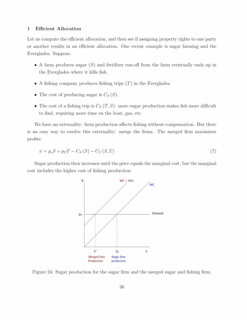
Sugar production then increases until the price equals the marginal cost, but the marginal

cost includes the higher cost of fishing production:

MC

S

Ps

$

Demand

Merged firmProduction

Sugar firmproduction

MC + MD

S∗ S0

Figure 24: Sugar production for the sugar firm and the merged sugar and fishing firm.

36

The merged firm produces the socially efficient amount of sugar (S∗), taking into account

the marginal cost of production including the fishing costs.

Notice that since supply equals demand:

Ps =dCs (S)

dS+

dCT (S, T )

dS(8)

2 Fishing company owns the property right

Suppose now the fishing company can charge the farmer for fertilizer runoff. Suppose the

fishing company charges P ′ for each unit of sugar produced.

NOTE: the price should always be made in terms of the quantity of the good or bad

causing the externality. Here we should charge per unit of fertilizer emitted. It may be easy

for example for the farmer to find a substitute for fertilizer and produce nearly as much

sugar. But the producer has no incentive to do this because of the tax. Similarly, the taxing

is not as efficient as taxing pollution for pollution reduction. But here we abstract from this

issue.

Now how much runoff will the fishing company “supply”? The fishing company allows

the sugar farmer to supply and additional unit of sugar if the revenues gained (P ′) exceed

the loss of profits that results from the sugar production. Otherwise it would be better to

deny the farmer access and produce fish at a lower cost. Let MD be the “marginal damage”

or the increase in costs to fishing caused by a small increase in sugar production. Then the

supply curve is:

Supply =dCT (S, T )

dT= MD (S) (9)

Now how much sugar production will the farmer “demand” to produce? Recall the farmer

gets Ps in revenue per unit of sugar and already faces MC (S) in costs per unit. Now she

will produce if the marginal profits exceed the cost of producing. Hence the sugar farmer’s

demand curve is:

Demand = Ps −MC (S) = Ps −dCs (S)

dS(10)

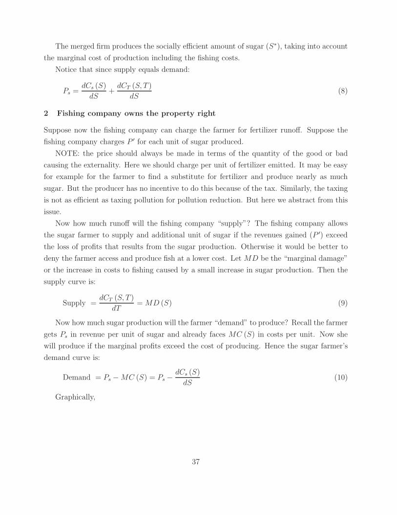
Graphically,

37

S

P’

P’

MD = dCt(S,T)ds

S0S∗SL

MC = Ps - MC(s)

SH

P’>MD

P’>MC

Figure 25: Market for runoff.

If payment is P ′ = 0, the firm produces S0, but has an incentive to reduce production if

the fishing company charges for runoff. At SH > S∗, the sugar farmer has negative marginal

profits. For unit SH , he receives Ps revenue less MC (SH) costs. But this is less than the P ′

the sugar farmer must pay the fishing company. Thus the sugar farmer reduces production.

At SL < S∗, the fishing company could make more profits by allowing runoff. The runoff

cost the firm only MD (SL) in lost fishing profits, but that is more than made up for by the

P ′ in payments from the sugar farm.

Returning to the math, at the equilibrium, supply equals demand so:

Demand = Ps −MC (S) = Supply = MD (11)

Ps −MC (S) = MD (S) (12)

Ps = MC (S) +MD (S) (13)

Ps =dCs (S)

dS+

dCT (S, T )

dS(14)

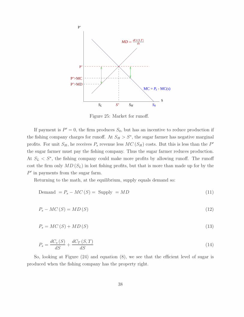
So, looking at Figure (24) and equation (8), we see that the efficient level of sugar is

produced when the fishing company has the property right.

38

S

$

Demand

EfficientProduction

Sugar Productionabsent payments

P’

=dCs(S)

ds +P′

Ps

MC =C′

s(S)

S∗ S0

MC =dCs(S)

ds +dCt (S)

ds

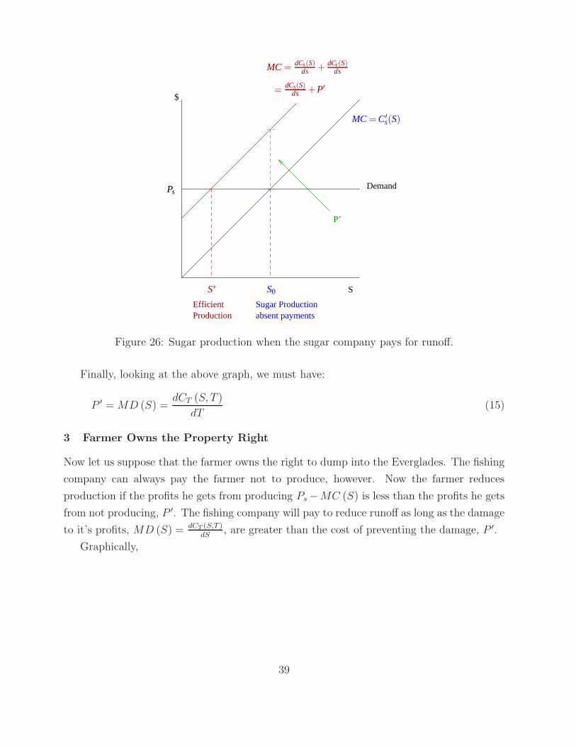
Figure 26: Sugar production when the sugar company pays for runoff.

Finally, looking at the above graph, we must have:

P ′ = MD (S) =dCT (S, T )

dT(15)

3 Farmer Owns the Property Right

Now let us suppose that the farmer owns the right to dump into the Everglades. The fishing

company can always pay the farmer not to produce, however. Now the farmer reduces

production if the profits he gets from producing Ps−MC (S) is less than the profits he gets

from not producing, P ′. The fishing company will pay to reduce runoff as long as the damage

to it’s profits, MD (S) = dCT (S,T )dS

, are greater than the cost of preventing the damage, P ′.

Graphically,

39

P’

P’

S

profitssugar profits

Fishing Co.

S∗ S0

MD =dCt(S,T )

ds

MC = Ps −MC(s)

SHSL

Fishing Co. WTPmore than sugarWTP less than

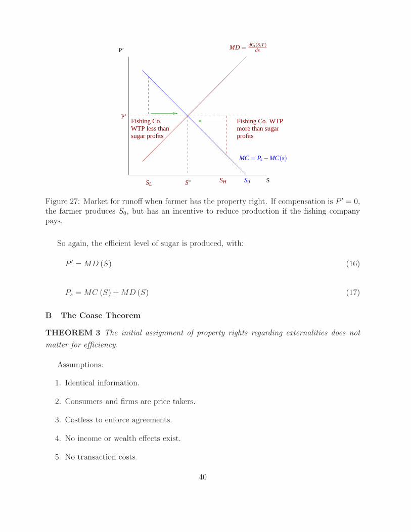
Figure 27: Market for runoff when farmer has the property right. If compensation is P ′ = 0,the farmer produces S0, but has an incentive to reduce production if the fishing companypays.

So again, the efficient level of sugar is produced, with:

P ′ = MD (S) (16)

Ps = MC (S) +MD (S) (17)

B The Coase Theorem

THEOREM 3 The initial assignment of property rights regarding externalities does not

matter for efficiency.

Assumptions:

1. Identical information.

2. Consumers and firms are price takers.

3. Costless to enforce agreements.

4. No income or wealth effects exist.

5. No transaction costs.

40

The Coase theorem is closely related to the welfare theorems, and shows that, once

property rights are established, the welfare theorems hold again and efficiency results. As

is the case with the welfare theorems, we cannot say anything about the distribution of

wealth. When property rights are assigned to the farmer the farmer is richer and the fishing

company’s shareholders are poorer (and vice versa). However, as is the case with the welfare

theorems, we can always make some transfers of resources (including the property rights over

the externality) so as to get any efficient outcome.

Definition 18 POLLUTER PAYS PRINCIPLE. Common environmental law principle that

makes the polluter pay for the damage caused by pollution.

The Coase theorem shows clearly that principles like the “polluter pays principle” are

really about distribution, not efficiency. They are also not about reducing pollution as no

matter who pays, pollution is reduced by the same amount.

Suppose now the government does not formally allocate a property right. Then the

property right is often in the polluter’s hands. In the absence of compensation, the farmer

will produce S0 and pollute.

Some use the Coase theorem to advocate that government regulation of externalities is

unnecessary. Just allow the farmer and fishing company to negotiate among themselves,

and an efficient outcome will result through mergers and/or side payments. One difficulty

with this idea is that transaction costs are often fairly high. Consider a set of n farmers,

and suppose it is not immediately clear which farmer the run off came from. It may be

prohibitively difficult to organize a set of side payments. However, in small groups the Coase

theorem is often very relevant. It is usually simpler and more straightforward to negotiate

with your neighbor over the level of noise, then to get a noise ordinance passed. The 2010

Nobel prize was for wor

C Numerical Example

Sugar farmer’s costs:

Cs (S) = S2 + 8 (18)

MCs (S) =dCs (S)

ds= 2S (19)

41

Fishing company’s costs:

CT (T, S) = T 2 + TS + 4 (20)

MCT (T, S) =dCT (T, S)

dT= 2T + S (21)

MDS (T, S) =dCT (T, S)

dS= T (22)

The prices are PS = 11, PT = 10.

To see the efficient allocation, we solve the problem of the merged firm:

max π = PsS + PTT − CS (S)− CT (S, T ) , (23)

max π = 11S + 10T − S2− 8− T 2

− TS − 4. (24)

To solve this problem, we can either take the derivatives with respect to T and S and set

them equal to zero, or use equation (8):

Ps =dCs (S)

dS+

dCT (S, T )

dS(25)

11 = 2S + T, (26)

Of course price equals marginal cost for the fishing trip production:

10 = PT = MCT (T, S) = 2T + S. (27)

Solving for S gives:

S = 10− 2T (28)

Plugging into (26) results in:

11 = 2 (10− 2T ) + T → T = 3. (29)

S = 10− 2 · 3 = 4. (30)

42

So it is efficient to produce 4 units of sugar and 3 trips, with the profit of the merged

firm being:

π = 11S + 10T − S2− 8− T 2

− TS − 4, (31)

π = 11 · 4 + 10 · 3− 42 − 8− 32 − 4 · 3− 4 = 25. (32)

Now do the profits with no property rights, in which case price equals marginal cost for

each firm. For the sugar farm,

11 = Ps =dCs (S)

dS= 2S → S = 5.5 (33)

So we have too much sugar production. Profits are:

πs = 11 · 5.5− 5.52 − 8 = 22.25 (34)

For the fishing company, price equals marginal cost as well:

PT = 10 =dCT (T, S)

dT= 2T + S = 2 · T + 5.5, (35)

10 = 2T + 5.5 → T = 2.25 (36)

So we have too little fishing trips. Profits are:

π = 10 · 2.25− 2.252 − 2.25 · 5.5− 4 = 1.0625. (37)

Total profits between the two firms are certainly less than the merged firm.

Finally, if property rights are assigned to either the farmer or the fishing company, we

have:

P ′ = MDS (T, S) =dCT (T, S)

dS= T = 3, (38)

since the efficient number of fishing trips was 3.

If the property rights are assigned to the fishing company, profits are:

πS = PsS − P ′S − Cs (S) = 11 · 4− 3 · 4− 42 − 8 = 8. (39)

43

πT = PTT + P ′S − CT (T, S) = 10 · 3 + 3 · 4− 32 − 3 · 4− 4 = 17. (40)

If the property rights are assigned to the farmer, we again have S = 4 and T = 3, so:

πS = PsS + P ′ (5.5− S)− Cs (S) = 11 · 4 + 3 · 4− 42 − 8 = 24.5. (41)

πT = PTT − P ′ (5.5− S)− CT (T, S) = 10 · 3− 3 · 1.5− 32 − 3 · 4− 4 = 0.5. (42)

So the property rights affects the distribution of profits but not the total.

D Conclusions

When the government bought some land in Florida from sugar farmers, with the purpose

of restoring the Everglades, we saw the Coase theorem in action. Despite the fact that the

polluter didn’t pay (and instead was compensated), water flow in the Everglades should

increase, benefiting many.

II Pigouvian Taxes

A Efficient Pollution Taxes: one polluter

Suppose now that, due to transactions costs, it is difficult for the farmer and the fisher to

negotiate a merger, or a set of side payments on their own. Perhaps many fishing company’s

exist, or perhaps instead of fishing companies we have recreational fisher’s, who have difficulty

organizing.

One strategy is for the government to impose a tax on the sugar farm for polluting.

Let t now be the tax on the polluting activity, charged to the sugar farm and paid to the

government. It is clear from equation (16) and Figure 28 that the efficient tax would be to

tax the sugar farm t = P ′ = MD per unit of S:

t = P ′ = MD (S) (43)

44

$

Demand

EfficientProduction

Sugar Productionabsent payment

t

Ps + t

Ps

MC =C′

s(S)

S∗ S0

MC =dCs(S)

ds +dCt (S,T)

ds

=dCs(S)

ds + t

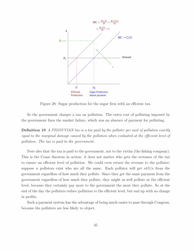
Figure 28: Sugar production for the sugar firm with an efficient tax.

So the government charges a tax on pollution. The extra cost of polluting imposed by

the government fixes the market failure, which was an absence of payment for polluting.

Definition 19 A PIGOUVIAN tax is a tax paid by the polluter per unit of pollution exactly

equal to the marginal damage caused by the pollution when evaluated at the efficient level of

pollution. The tax is paid to the government.

Note also that the tax is paid to the government, not to the victim (the fishing company).

This is the Coase theorem in action: it does not matter who gets the revenues of the tax

to ensure an efficient level of pollution. We could even return the revenue to the polluter:

suppose n polluters exist who are all the same. Each polluter will get ntS/n from the

government regardless of how much they pollute. Since they get the same payment from the

government regardless of how much they pollute, they might as well pollute at the efficient

level, because they certainly pay more to the government the more they pollute. So at the

end of the day the polluters reduce pollution to the efficient level, but end up with no change

in profits.

Such a payment system has the advantage of being much easier to pass through Congress,

because the polluters are less likely to object.

45

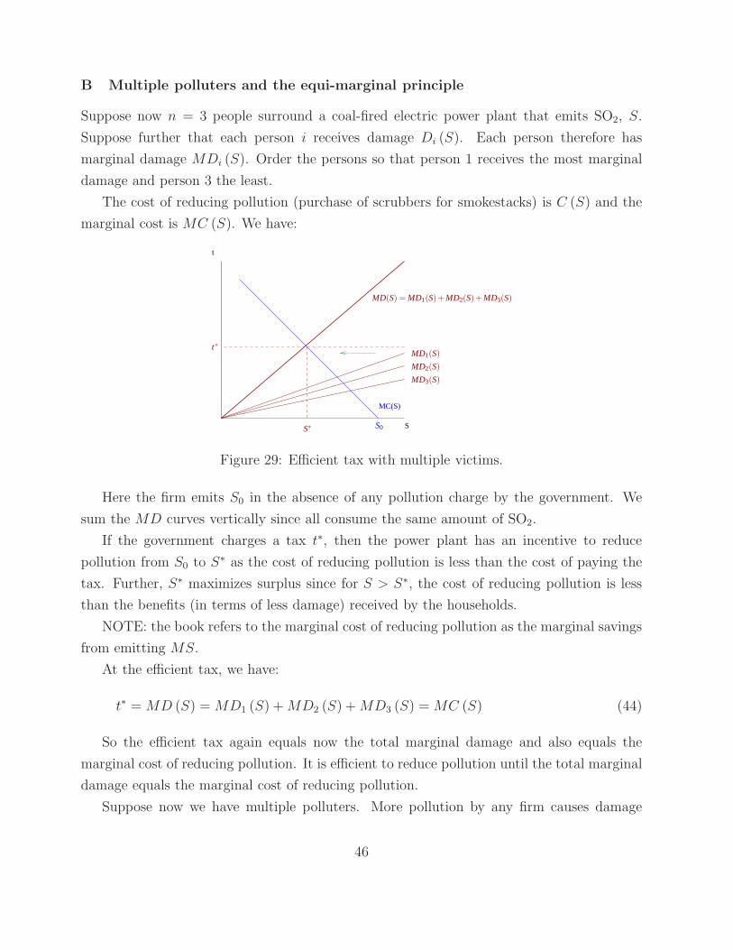
B Multiple polluters and the equi-marginal principle

Suppose now n = 3 people surround a coal-fired electric power plant that emits SO2, S.

Suppose further that each person i receives damage Di (S). Each person therefore has

marginal damage MDi (S). Order the persons so that person 1 receives the most marginal

damage and person 3 the least.

The cost of reducing pollution (purchase of scrubbers for smokestacks) is C (S) and the

marginal cost is MC (S). We have:

t

S

MC(S)

S0

t∗

S∗

MD(S) = MD1(S)+MD2(S)+MD3(S)

MD3(S)

MD2(S)

MD1(S)

Figure 29: Efficient tax with multiple victims.

Here the firm emits S0 in the absence of any pollution charge by the government. We

sum the MD curves vertically since all consume the same amount of SO2.

If the government charges a tax t∗, then the power plant has an incentive to reduce

pollution from S0 to S∗ as the cost of reducing pollution is less than the cost of paying the

tax. Further, S∗ maximizes surplus since for S > S∗, the cost of reducing pollution is less

than the benefits (in terms of less damage) received by the households.

NOTE: the book refers to the marginal cost of reducing pollution as the marginal savings

from emitting MS.

At the efficient tax, we have:

t∗ = MD (S) = MD1 (S) +MD2 (S) +MD3 (S) = MC (S) (44)

So the efficient tax again equals now the total marginal damage and also equals the

marginal cost of reducing pollution. It is efficient to reduce pollution until the total marginal

damage equals the marginal cost of reducing pollution.

Suppose now we have multiple polluters. More pollution by any firm causes damage

46

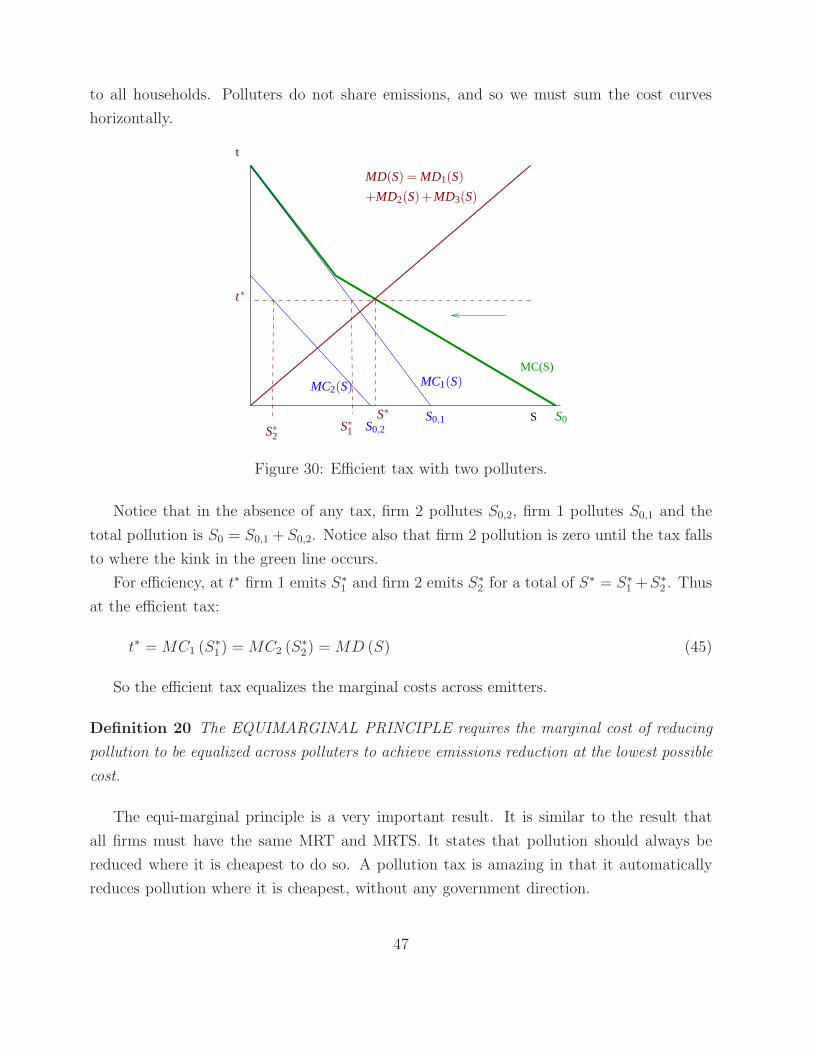
to all households. Polluters do not share emissions, and so we must sum the cost curves

horizontally.

MC(S)

t

S S0

t∗

S0,1

MC1(S)MC2(S)

S0,2

S∗

S∗2S∗1

+MD2(S)+MD3(S)

MD(S) = MD1(S)

Figure 30: Efficient tax with two polluters.

Notice that in the absence of any tax, firm 2 pollutes S0,2, firm 1 pollutes S0,1 and the

total pollution is S0 = S0,1 + S0,2. Notice also that firm 2 pollution is zero until the tax falls

to where the kink in the green line occurs.

For efficiency, at t∗ firm 1 emits S∗

1 and firm 2 emits S∗

2 for a total of S∗ = S∗

1 +S∗

2 . Thus

at the efficient tax:

t∗ = MC1 (S∗

1) = MC2 (S∗

2) = MD (S) (45)

So the efficient tax equalizes the marginal costs across emitters.

Definition 20 The EQUIMARGINAL PRINCIPLE requires the marginal cost of reducing

pollution to be equalized across polluters to achieve emissions reduction at the lowest possible

cost.

The equi-marginal principle is a very important result. It is similar to the result that

all firms must have the same MRT and MRTS. It states that pollution should always be

reduced where it is cheapest to do so. A pollution tax is amazing in that it automatically

reduces pollution where it is cheapest, without any government direction.

47

Suppose for example that MC (S1) < t < MC (S2). Then for firm 2, paying the tax is

cheaper than reducing pollution, whereas for firm 1 the opposite is true. Therefore, firm 1

will reduce pollution but not firm 2. But firm 1 is where it is cheapest to reduce emissions! In

turn, the decrease in emissions by firm pushes up firm 1’s marginal cost of reducing further,

until the tax equals the marginal cost.

The equi-marginal principle we will see later is not satisfied by most kinds of environmen-

tal regulation. This is because most regulation requires all firms to reduce emissions by the

same amount. Consider the Kyoto protocol which requires all countries to reduce emissions

by 7% below 1990 levels. This certainly does not equalize marginal costs.

Sometimes, the government tries to get around this problem in a blunt way. Consider

VINTAGE DIFFERENTIATED REGULATION, which gives weaker emissions reduction

requirements to older cars or factories. Indeed, coal fired power plants have such vintage

differentiation in their regulations: the New Source Review law effectively means that newer

(or retrofitted) plants are subject to tighter emissions targets. But problems arise.

• First it may be cheaper to reduce emissions in older plants.

• It requires a lot of knowledge on the part of the government to set the target differently

for each vintage of the plant, whereas the tax does this automatically.

• Firms have an incentive not to upgrade their plants, or to declare their upgrades are

“routine maintenance,” to preserve their status as older vintages.

C Imperfect Competition

A monopolist has an incentive to restrict goods production, so as to drive up the price and

increase profits. This has the side benefit of also reducing pollution. Thus, we might suspect

a Pigouvian tax (equal to the marginal damage), might restrict output too much (below the

efficient level).

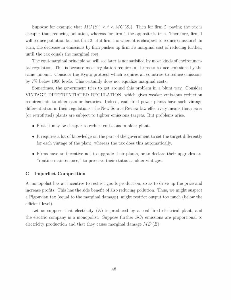
Let us suppose that electricity (E) is produced by a coal fired electrical plant, and

the electric company is a monopolist. Suppose further SO2 emissions are proportional to

electricity production and that they cause marginal damage MD (E).

48

P

E

MC(E)+MD(E)

Demand=MWTP(E)MR

MC(E)

Pm + t

P∗

Et

Pm

Em E∗

Figure 31: Electricity production with a monopolist electricity producer.

It is efficient to produce the quantity of electricity where demand or MWTP equal the

total marginal cost, including both the private marginal cost of producing electricity and the

social cost which is the marginal damage to the air breathers. This is E∗.

In the absence of a tax, the monopolist ignores the marginal damage and considers only

his private costs. Further, the monopolist knows that by restricting production he can drive

up the price and produce more. Thus he produces where the marginal revenue (the extra

revenue from producing one more unit, taking into account the resulting price decrease)

equals the private marginal cost. This is Em with price Pm. Note that Em is already less

than the efficient E, and pollution is already lower than the efficient level.

Now if the government steps in with the Pigouvian tax, it will drive down electricity

production still further, reducing surplus again. One could instead regulate the price the

monopoly charges, here P ∗ including tax. But regulating a price of P ∗ is not a Pigouvian

tax.

III Command and Control

Definition 21 COMMAND-AND-CONTROL regulation specifies how pollution is to be re-

duced.

Now this definition is somewhat imprecise, as some command-and-control regulation

specifies how pollution is to be reduced in great detail, while other command-and-control

49

regulations allow some flexibility. All, however, result in lower welfare than tax based regu-

lation, however. This is because command-and-control does not reduce pollution in the least

costly way, whereas tax regulation does.

Consider two basic types:

• EMISSIONS STANDARD: Require emissions at every factory/plant not to exceed a

standard.

• TECHNOLOGY STANDARD: Require production using a technology which limits

pollution per unit of output.

A Emissions Standard

Suppose we require all electric power plants (coal fired or otherwise), to limit emissions to

e. We will choose e so that the total emitted by all firms is the efficient level of pollution.

Since we have two firms, e+ e = e∗ and so e = e∗/2.

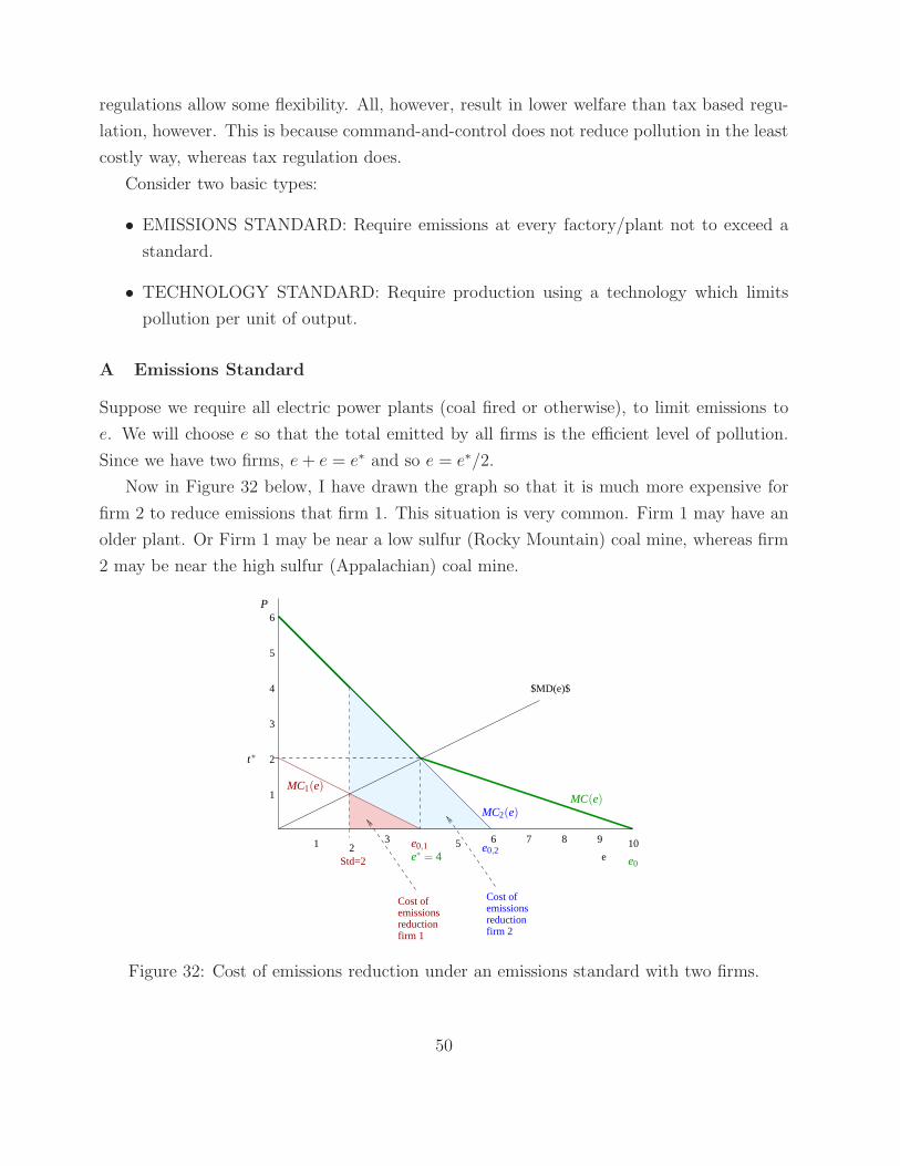
Now in Figure 32 below, I have drawn the graph so that it is much more expensive for

firm 2 to reduce emissions that firm 1. This situation is very common. Firm 1 may have an

older plant. Or Firm 1 may be near a low sulfur (Rocky Mountain) coal mine, whereas firm

2 may be near the high sulfur (Appalachian) coal mine.

e

$MD(e)$

Cost of emissionsreductionfirm 1

1

2

3

4

6

5

1 2Std=2

3 5 6 7

Cost of

9 108

emissionsreductionfirm 2

e∗ = 4 e0

MC(e)

e0,2

MC2(e)

MC1(e)

e0,1

t∗

P

Figure 32: Cost of emissions reduction under an emissions standard with two firms.

50

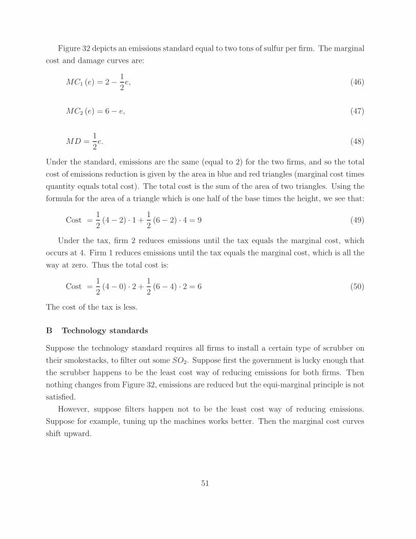
Figure 32 depicts an emissions standard equal to two tons of sulfur per firm. The marginal

cost and damage curves are:

MC1 (e) = 2−1

2e, (46)

MC2 (e) = 6− e, (47)

MD =1

2e. (48)

Under the standard, emissions are the same (equal to 2) for the two firms, and so the total

cost of emissions reduction is given by the area in blue and red triangles (marginal cost times

quantity equals total cost). The total cost is the sum of the area of two triangles. Using the

formula for the area of a triangle which is one half of the base times the height, we see that:

Cost =1

2(4− 2) · 1 +

1

2(6− 2) · 4 = 9 (49)

Under the tax, firm 2 reduces emissions until the tax equals the marginal cost, which

occurs at 4. Firm 1 reduces emissions until the tax equals the marginal cost, which is all the

way at zero. Thus the total cost is:

Cost =1

2(4− 0) · 2 +

1

2(6− 4) · 2 = 6 (50)

The cost of the tax is less.

B Technology standards

Suppose the technology standard requires all firms to install a certain type of scrubber on

their smokestacks, to filter out some SO2. Suppose first the government is lucky enough that

the scrubber happens to be the least cost way of reducing emissions for both firms. Then

nothing changes from Figure 32, emissions are reduced but the equi-marginal principle is not

satisfied.

However, suppose filters happen not to be the least cost way of reducing emissions.

Suppose for example, tuning up the machines works better. Then the marginal cost curves

shift upward.

51

1

2

3

4

6

5

1 23 5 6 7 8 9

Std=2

10

Se∗ = 4

MC(e)

e0e0,2

MD(e)

t∗

e0,1

MC1(e)

MC2(e)

P

MC′(e)

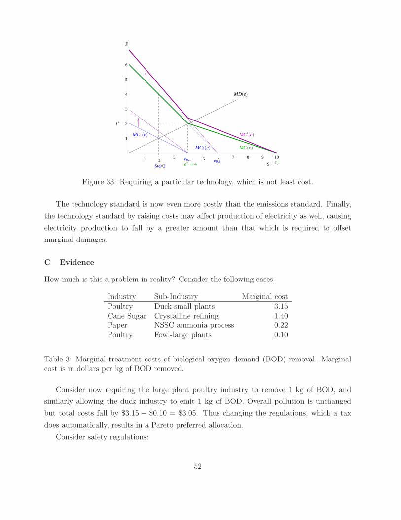
Figure 33: Requiring a particular technology, which is not least cost.

The technology standard is now even more costly than the emissions standard. Finally,

the technology standard by raising costs may affect production of electricity as well, causing

electricity production to fall by a greater amount than that which is required to offset

marginal damages.

C Evidence

How much is this a problem in reality? Consider the following cases:

Industry Sub-Industry Marginal costPoultry Duck-small plants 3.15Cane Sugar Crystalline refining 1.40Paper NSSC ammonia process 0.22Poultry Fowl-large plants 0.10

Table 3: Marginal treatment costs of biological oxygen demand (BOD) removal. Marginalcost is in dollars per kg of BOD removed.

Consider now requiring the large plant poultry industry to remove 1 kg of BOD, and

similarly allowing the duck industry to emit 1 kg of BOD. Overall pollution is unchanged

but total costs fall by $3.15 − $0.10 = $3.05. Thus changing the regulations, which a tax

does automatically, results in a Pareto preferred allocation.

Consider safety regulations:

52

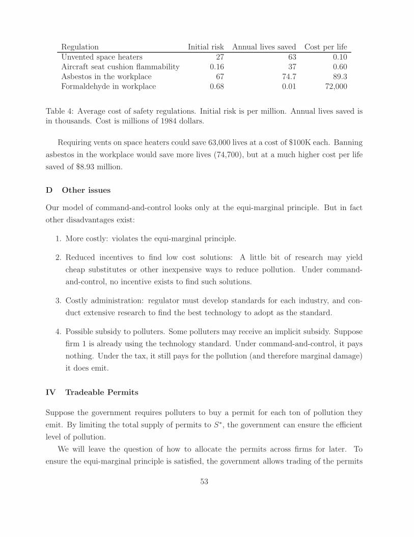
Regulation Initial risk Annual lives saved Cost per lifeUnvented space heaters 27 63 0.10Aircraft seat cushion flammability 0.16 37 0.60Asbestos in the workplace 67 74.7 89.3Formaldehyde in workplace 0.68 0.01 72,000

Table 4: Average cost of safety regulations. Initial risk is per million. Annual lives saved isin thousands. Cost is millions of 1984 dollars.

Requiring vents on space heaters could save 63,000 lives at a cost of $100K each. Banning

asbestos in the workplace would save more lives (74,700), but at a much higher cost per life

saved of $8.93 million.

D Other issues

Our model of command-and-control looks only at the equi-marginal principle. But in fact

other disadvantages exist:

1. More costly: violates the equi-marginal principle.

2. Reduced incentives to find low cost solutions: A little bit of research may yield

cheap substitutes or other inexpensive ways to reduce pollution. Under command-

and-control, no incentive exists to find such solutions.

3. Costly administration: regulator must develop standards for each industry, and con-

duct extensive research to find the best technology to adopt as the standard.

4. Possible subsidy to polluters. Some polluters may receive an implicit subsidy. Suppose

firm 1 is already using the technology standard. Under command-and-control, it pays

nothing. Under the tax, it still pays for the pollution (and therefore marginal damage)

it does emit.

IV Tradeable Permits

Suppose the government requires polluters to buy a permit for each ton of pollution they

emit. By limiting the total supply of permits to S∗, the government can ensure the efficient

level of pollution.

We will leave the question of how to allocate the permits across firms for later. To

ensure the equi-marginal principle is satisfied, the government allows trading of the permits

53

in an open market. Each firm will buy a permit if the price of the permit is less than

the marginal cost of reducing emissions. Thus the demand for permits equals the marginal

cost of emissions reduction. The supply is of course fixed by the government at S∗. The

equilibrium price of permits satisfies:

P = MD (e∗) = MC1 (e∗) = MC2 (e

∗) . (51)

Permit

Price

MC(e)

e0

P∗

e0,1e

MC1(e)MC2(e)

e0,2

e∗

e∗2e∗1

MD(e)

Figure 34: Equilibrium permit price and emissions in the tradeable permit market. Bothemissions in tons and the quantity of permits (one permit per ton) are denoted by e.

So the tradeable permit regulation also results in the efficient allocation, with the equi-

librium permit price being the same as the tax rate P = t. The problem with standards is

not so much limiting a firm’s emissions, as not allowing the firm to trade that right.

V Liability

Suppose we make the firm liable for any damage caused. If only one firm exists, this is easy.

But if multiple firms exist, which firm emitted first (causing low marginal damages) and

which firm emitted last (causing higher marginal damages since the second firm is adding

to the already high emissions)? Suppose we resolve this problem by changing firm 1 all

marginal damages given firm 2’s emissions.

54

$MC(e)$$MC_1 (e) $

liability$

e0e0,1

MC2(e)

e0,2

e∗

MD(e)=marginal

e∗2 e∗1 e

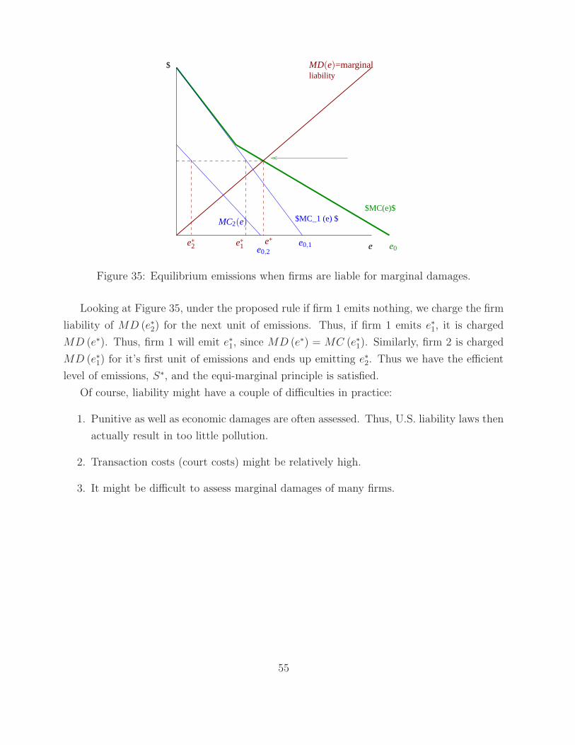
Figure 35: Equilibrium emissions when firms are liable for marginal damages.

Looking at Figure 35, under the proposed rule if firm 1 emits nothing, we charge the firm

liability of MD (e∗2) for the next unit of emissions. Thus, if firm 1 emits e∗1, it is charged

MD (e∗). Thus, firm 1 will emit e∗1, since MD (e∗) = MC (e∗1). Similarly, firm 2 is charged

MD (e∗1) for it’s first unit of emissions and ends up emitting e∗2. Thus we have the efficient

level of emissions, S∗, and the equi-marginal principle is satisfied.

Of course, liability might have a couple of difficulties in practice:

1. Punitive as well as economic damages are often assessed. Thus, U.S. liability laws then

actually result in too little pollution.

2. Transaction costs (court costs) might be relatively high.

3. It might be difficult to assess marginal damages of many firms.

55