dendrite tracking in microscopic images using minimum...
TRANSCRIPT
Dendrite Tracking in Microscopic Images usingMinimum Spanning Trees and Localized E-M
Francois Fleuret and Pascal FuaCVLAB – EPFL
March 27, 2006
Technical Report EPFL/CVLAB2006.02
Abstract
We describe in this document our preliminary results regarding thetracking of dendrites spreading from a neuron in confocal microscope im-ages. When using a small number of image layers, we obtain good resultsby combining a EM-based local estimate of the probability that an imagepixel belongs to a neuron filament with the global tree properties of thecomplete set of dendrites. The optimal tree is obtained with a modifiedminimum-spanning tree procedure. We will argue that this approach ex-tends naturally to the complete data volume and should give even betterresults.
1 Introduction
Full reconstruction of neuron morphology is of fundamental interest for theanalysis and understanding of their functioning. So far, most commercialproducts such as Neurolucida1, Imaris2 or Metamorph3 provide with pow-erful interfaces to reconstruct dendritic trees but relies heavily on manualoperations for initialization and re-initialization of the procedures able tofollow neuron filaments along in the tissue.
In its most basic form, the problem consists of processing a stack ofpictures produced by a confocal microscope, each of them showing a slice
1http://www.microbrightfield.com/prod-nl.htm2http://www.bitplane.com/products/imaris/imaris product.shtml3http://www.moleculardevices.com/pages/software/metamorph.html
1
EPFL/CVLAB2006.02 Dendritic Tree Tracking
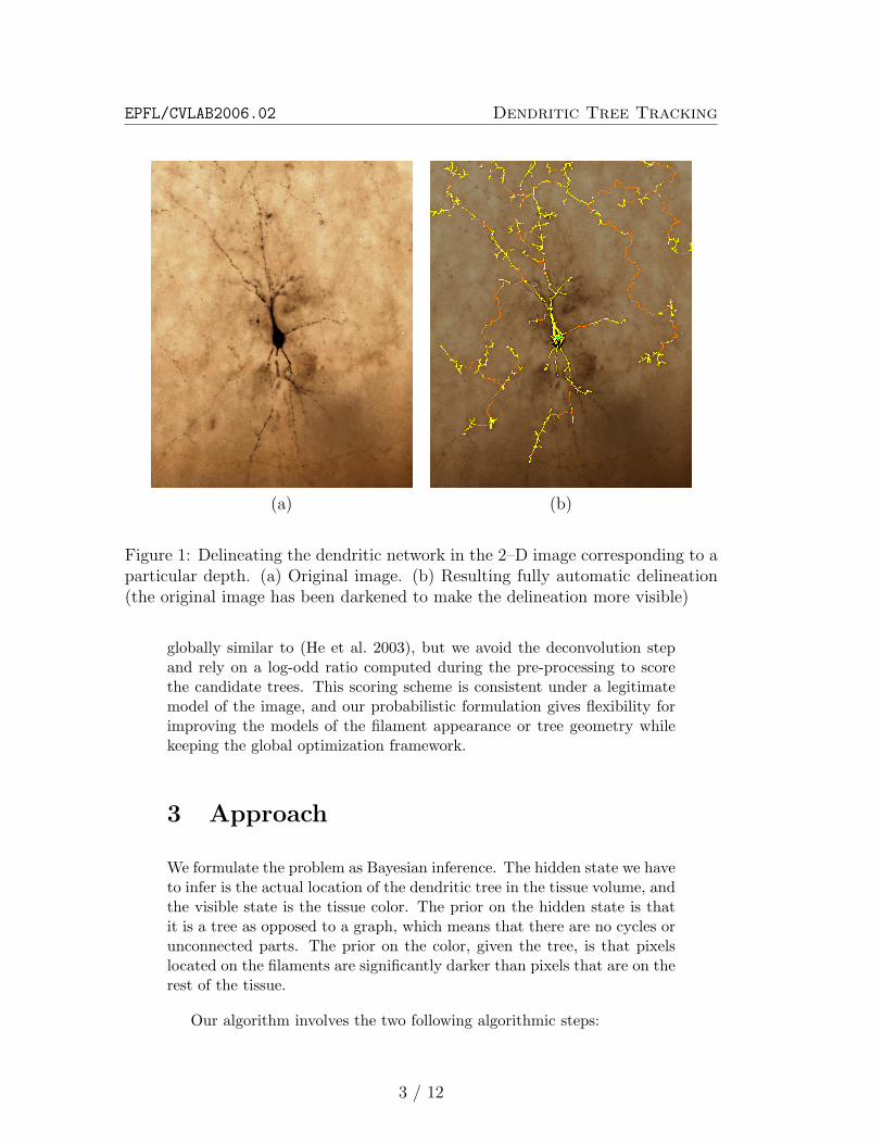
of the same piece of tissue at a different depth. It is transparent enoughso that these pictures can be acquired by simply changing the focal plane.Since dye was injected into the cell to be reconstructed, it became opaqueto light, while the rest of the tissue retains its original color. Finally, theneuron and its extension appear on the picture as dark filaments as showninFig. 1(a).
To automatically delineate the dendrites in such images, the main dif-ficulty comes from the multiple discontinuities in the filaments, which aredue to inhomogeneities in their thickness. For example, the presence ofsynapses locally increases the diameter of a filament and results in seriesof dots such as those that are clearly visible in Fig. 2(a).
Thus, simply following the darkest paths in the picture cannot be ex-pected to yield good results. A successful strategy has to involve both thelocal characterization of the filament-like parts of the pictures and moreglobal modeling of dendritic networks.
In this report, we propose such a strategy, similar to (He et al. 2003),which combines local color-based estimate of the probability that an imagepixel belongs to a filament with the global tree properties of the completeset of filaments. We avoid having to de-noise the image by keeping aprobabilistic semantic in the result of the segmentation step. Our methodproduces results such as those of Fig. 1(b), which compare favorably tomanual delineation. So far, we have only tested our approach in the 2–Dcase using a small number of layers. However, we expect our approachto naturally extend to the full data volume, where it should perform evenbetter.
2 Related Work
Reconstruction of large networks of filaments is an important subject atthe interface between medical imaging and computer vision. Its two mainapplications are the reconstruction of brain vascular networks (Kirbas &Quek 2003, Krissian et al. 2004) and neuron dendritic trees.
For clean high-resolution images, techniques can rely on the continuityof the structures to follow and take advantage of sophisticated 3D mod-els of the filaments (Shen et al. 2001, Al-Kofahi et al. 2002). However,since we want to deal here with pictures of lower quality, where structuresmay appear to be discontinuous due to noise, we propose to use a tech-nique based on the minimal spanning tree technique. This optimizationscheme has been used in computer vision since the 80s, for instance forroad-tracking in satellite images (Fischler et al. 1987). Our approach is
2 / 12
EPFL/CVLAB2006.02 Dendritic Tree Tracking
(a) (b)
Figure 1: Delineating the dendritic network in the 2–D image corresponding to aparticular depth. (a) Original image. (b) Resulting fully automatic delineation(the original image has been darkened to make the delineation more visible)
globally similar to (He et al. 2003), but we avoid the deconvolution stepand rely on a log-odd ratio computed during the pre-processing to scorethe candidate trees. This scoring scheme is consistent under a legitimatemodel of the image, and our probabilistic formulation gives flexibility forimproving the models of the filament appearance or tree geometry whilekeeping the global optimization framework.
3 Approach
We formulate the problem as Bayesian inference. The hidden state we haveto infer is the actual location of the dendritic tree in the tissue volume, andthe visible state is the tissue color. The prior on the hidden state is thatit is a tree as opposed to a graph, which means that there are no cycles orunconnected parts. The prior on the color, given the tree, is that pixelslocated on the filaments are significantly darker than pixels that are on therest of the tissue.
Our algorithm involves the two following algorithmic steps:
3 / 12
EPFL/CVLAB2006.02 Dendritic Tree Tracking
Table 1: Notation used in Sections 3.1 and 3.2
I(x, y)
Image intensity at location (x, y);
Y (x, y)
Boolean random process standing for the presenceof a filament at pixel (x, y);
W (x, y)
Boolean random process standing for the visibilityof filament (if present) at pixel (x, y);
Z(x, y) = Y (x, y) W (y, x)
Boolean random process standing for the actualneuron-color coloration of pixel (x, y);
ξ(x, y) = P (Z = 1 | I(x, y))
Probability that a pixel is on a visible part of afilament given its color;
δ = P (Y = 1) and ε = P (W = 1)
The prior probability of the filament presence andfilament visibility.
1. Estimating the probability for every pixel to be on a filament, givenonly its intensity;
2. Building the optimal tree.
In the two following sections, we describe these individual steps.
3.1 Estimating the Probability of Belonging to aFilament
Our algorithm’s first step is to estimate the probability for every pixel tobelong to a filament given its color. As stated above, our basic assumptionis that a filament pixel is, in general, darker than a non-filament one. Note,however, that this is a local property as opposed to a global one. Forexample, in the images we experimented with, some areas were globallybrighter than others, presumably due to imaging artifacts. As a result,
4 / 12
EPFL/CVLAB2006.02 Dendritic Tree Tracking
(a) (b)
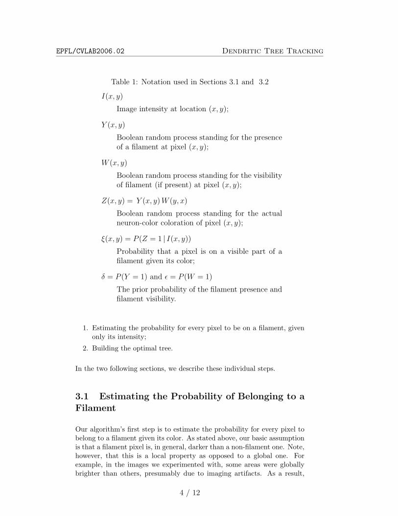
(c) (d)
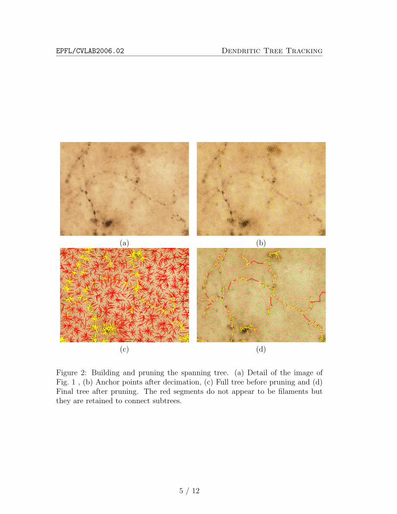
Figure 2: Building and pruning the spanning tree. (a) Detail of the image ofFig. 1 , (b) Anchor points after decimation, (c) Full tree before pruning and (d)Final tree after pruning. The red segments do not appear to be filaments butthey are retained to connect subtrees.
5 / 12
EPFL/CVLAB2006.02 Dendritic Tree Tracking
(a) (b) (c)
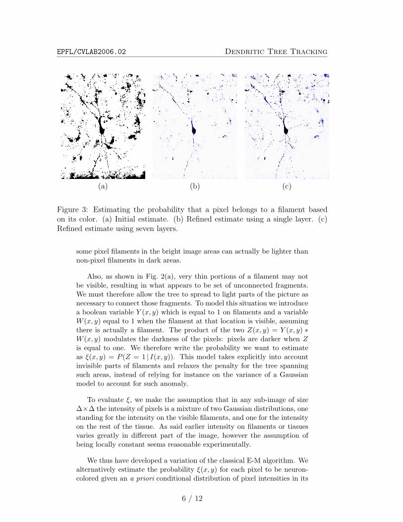
Figure 3: Estimating the probability that a pixel belongs to a filament basedon its color. (a) Initial estimate. (b) Refined estimate using a single layer. (c)Refined estimate using seven layers.
some pixel filaments in the bright image areas can actually be lighter thannon-pixel filaments in dark areas.
Also, as shown in Fig. 2(a), very thin portions of a filament may notbe visible, resulting in what appears to be set of unconnected fragments.We must therefore allow the tree to spread to light parts of the picture asnecessary to connect those fragments. To model this situation we introducea boolean variable Y (x, y) which is equal to 1 on filaments and a variableW (x, y) equal to 1 when the filament at that location is visible, assumingthere is actually a filament. The product of the two Z(x, y) = Y (x, y) ∗W (x, y) modulates the darkness of the pixels: pixels are darker when Zis equal to one. We therefore write the probability we want to estimateas ξ(x, y) = P (Z = 1 | I(x, y)). This model takes explicitly into accountinvisible parts of filaments and relaxes the penalty for the tree spanningsuch areas, instead of relying for instance on the variance of a Gaussianmodel to account for such anomaly.
To evaluate ξ, we make the assumption that in any sub-image of size∆×∆ the intensity of pixels is a mixture of two Gaussian distributions, onestanding for the intensity on the visible filaments, and one for the intensityon the rest of the tissue. As said earlier intensity on filaments or tissuesvaries greatly in different part of the image, however the assumption ofbeing locally constant seems reasonable experimentally.
We thus have developed a variation of the classical E-M algorithm. Wealternatively estimate the probability ξ(x, y) for each pixel to be neuron-colored given an a priori conditional distribution of pixel intensities in its
6 / 12

EPFL/CVLAB2006.02 Dendritic Tree Tracking
neighborhood, and then re-estimate this conditional intensity distributiongiven which pixels are considered to belong to filaments and which are not.
Thus, this can be divided in three parts:
1. Initialize ξ
This is done by setting this value to 1 where the intensity is morethan one standard deviation from the mean, where both mean andstandard deviation have been computed over the whole image;
2. Update the local modelsCompute for each pixel the conditional expectation and standarddeviation of the intensity inside and outside neuron filaments in aneighborhood of size ∆×∆. The cost of this estimation can be madeindependent from ∆ by using integral images;
3. Update ξ
Re-estimate ξ according to a Bayesian rule and Gaussian models. Goback to 2. until convergence.
Fig. 3(a) shows the initialization values. Fig. 3(b) depicts the resultingrefined probability image. To further improve the result, we can performthis computation on several layers of thin stack of images and take ξ tobe the maximum value at each (x, y) location, which yields the result ofFig. 3(c).
3.2 Computing the Optimal Tree
Let T be the set of pixels on the actual filament tree. We show in AppendixA that the log probability of observing the specific image I we use as input,given T , can be evaluated as
log P (I |T ) = Ψ0 +∑
(x,y)∈T
Ψ(x, y)
where
Ψ(x, y) = logP (I(x, y) |Y (x, y) = 1)P (I(x, y) |Y (x, y) = 0)
which can be computed from the estimate of ξ(x, y) = P (Z(x, y) = 1 | I(x, y))and the priors δ = P (Y = 1) and ε = P (W = 1) (see Appendix B).
7 / 12
EPFL/CVLAB2006.02 Dendritic Tree Tracking
Thus finding the maximum likelihood tree T reduces to finding the treet that maximizes
∑(x,y)∈t
Ψ(x, y) .
To this end, we have developed a greedy algorithm, which is a variationof the maximum spanning tree (Kruskal Jr. 1956, Prim 1957, Gower &Ross 1969, Zahn 1971). We first find a set of anchor points, which arelocal maxima of the ξ(x, y) probability defined in Section 3.1. We thenbuild the maximum likelihood tree that spans them.
1. Subsampling the set of pixelsThe purpose of this initial step is to reduce the cardinality of theset of pixels to process. We call the pixels remaining after that stepanchor points and they are chosen to be sufficiently dense on the areasof interest so that the optimal tree can be defined as a tree spanninga subset of these points.To select anchor points, we build a ranked list of all the pixel of theimage according to their Ψ value. We take the first element of thelist to be an anchor and remove from the list all other points withina radius ρ. We then iterate this process until the list is empty, whichyields results such as the one if Fig. 2(b).This process dramatically reduces the number of pixels to be consid-ered, while retaining all pixels at locations likely to be on a filament.
2. Building the TreeWe build the set of all edges of length less than 3ρ between anchorsand rank them according to the average value of Ψ along the segmentjoining them. We then consider them sequentially and add to the treeany edge which does not create a cycle in the resulting graph.This yields trees such as the one of Fig. 2(c). Note that due to the3ρ distance threshold, we may not be able to build a tree spanningall anchors. Non-connected anchors are considered as belonging topieces of pieces of filaments unrelated to the considered neuron.
3. Pruning optimallyGiven the optimal full tree spanning all the anchor points, we cancompute the global optimal subtree by removing all the anchors suchthat the integral of Ψ on the subtree it holds is negative (see figure 2(c) and (d) and 4). This can be done by ranking the anchors accordingto their discrete distance to the starting point, measured by how manyintermediate anchors between it and the starting point there are, andupdating that integral score by considering them sequentially.
8 / 12
EPFL/CVLAB2006.02 Dendritic Tree Tracking
8
origin
7
−3
−1
−1
2
6
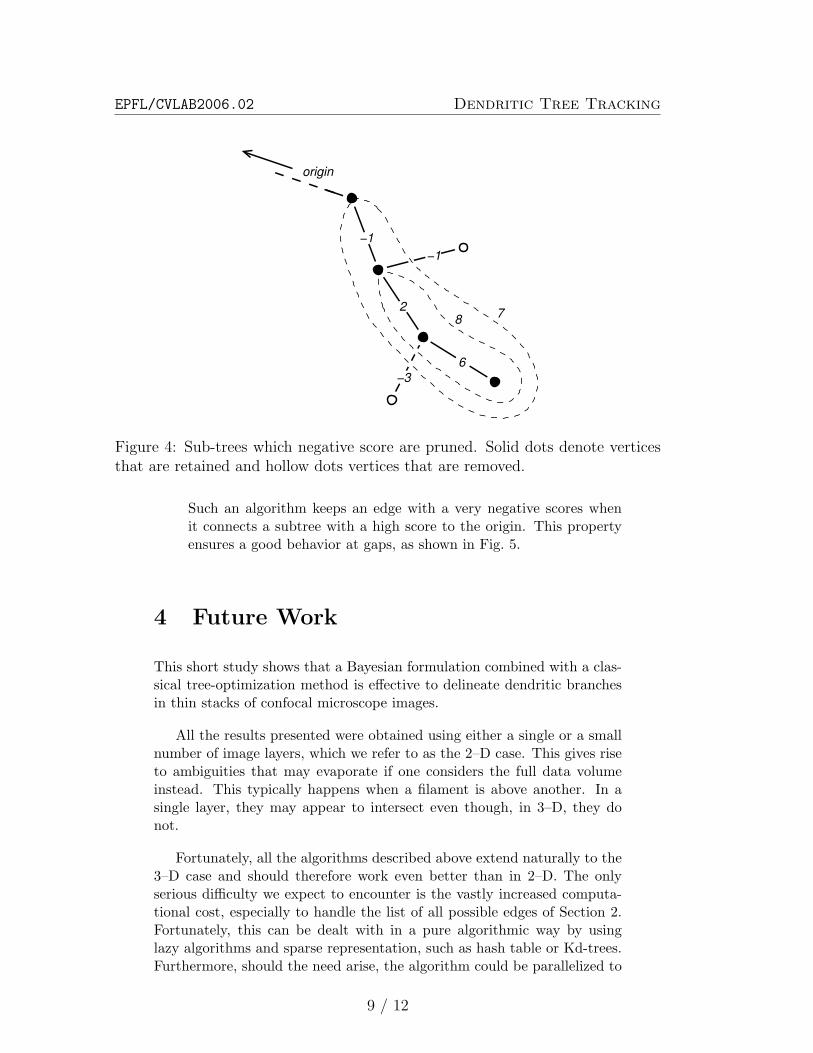
Figure 4: Sub-trees which negative score are pruned. Solid dots denote verticesthat are retained and hollow dots vertices that are removed.
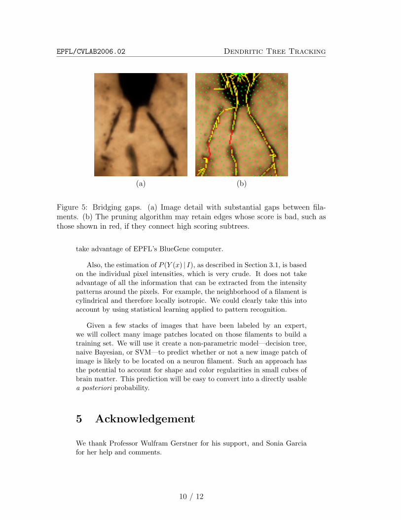
Such an algorithm keeps an edge with a very negative scores whenit connects a subtree with a high score to the origin. This propertyensures a good behavior at gaps, as shown in Fig. 5.
4 Future Work
This short study shows that a Bayesian formulation combined with a clas-sical tree-optimization method is effective to delineate dendritic branchesin thin stacks of confocal microscope images.
All the results presented were obtained using either a single or a smallnumber of image layers, which we refer to as the 2–D case. This gives riseto ambiguities that may evaporate if one considers the full data volumeinstead. This typically happens when a filament is above another. In asingle layer, they may appear to intersect even though, in 3–D, they donot.
Fortunately, all the algorithms described above extend naturally to the3–D case and should therefore work even better than in 2–D. The onlyserious difficulty we expect to encounter is the vastly increased computa-tional cost, especially to handle the list of all possible edges of Section 2.Fortunately, this can be dealt with in a pure algorithmic way by usinglazy algorithms and sparse representation, such as hash table or Kd-trees.Furthermore, should the need arise, the algorithm could be parallelized to
9 / 12
EPFL/CVLAB2006.02 Dendritic Tree Tracking
(a) (b)
Figure 5: Bridging gaps. (a) Image detail with substantial gaps between fila-ments. (b) The pruning algorithm may retain edges whose score is bad, such asthose shown in red, if they connect high scoring subtrees.
take advantage of EPFL’s BlueGene computer.
Also, the estimation of P (Y (x) | I), as described in Section 3.1, is basedon the individual pixel intensities, which is very crude. It does not takeadvantage of all the information that can be extracted from the intensitypatterns around the pixels. For example, the neighborhood of a filament iscylindrical and therefore locally isotropic. We could clearly take this intoaccount by using statistical learning applied to pattern recognition.
Given a few stacks of images that have been labeled by an expert,we will collect many image patches located on those filaments to build atraining set. We will use it create a non-parametric model—decision tree,naive Bayesian, or SVM—to predict whether or not a new image patch ofimage is likely to be located on a neuron filament. Such an approach hasthe potential to account for shape and color regularities in small cubes ofbrain matter. This prediction will be easy to convert into a directly usablea posteriori probability.
5 Acknowledgement
We thank Professor Wulfram Gerstner for his support, and Sonia Garciafor her help and comments.
10 / 12
EPFL/CVLAB2006.02 Dendritic Tree Tracking
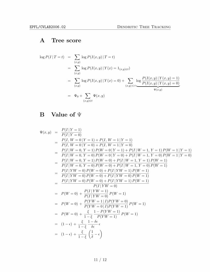
A Tree score
log P (I |T = t) =∑(x,y)
log P (I(x, y) |T = t)
=∑(x,y)
log P (I(x, y) |Y (x) = 1(x,y)∈t)
=∑(x,y)
log P (I(x, y) |Y (x) = 0) +∑
(x,y)∈ t
logP (I(x, y) |Y (x, y) = 1)P (I(x, y) |Y (x, y) = 0)︸ ︷︷ ︸
Ψ(x,y)
= Ψ0 +∑
(x,y)∈t
Ψ(x, y)
B Value of Ψ
Ψ(x, y) =P (I |Y = 1)P (I |Y = 0)
=P (I, W = 0 |Y = 1) + P (I, W = 1 |Y = 1)P (I, W = 0 |Y = 0) + P (I, W = 1 |Y = 0)
=P (I |W = 0, Y = 1)P (W = 0 |Y = 1) + P (I |W = 1, Y = 1)P (W = 1 |Y = 1)P (I |W = 0, Y = 0)P (W = 0 |Y = 0) + P (I |W = 1, Y = 0)P (W = 1 |Y = 0)
=P (I |W = 0, Y = 1)P (W = 0) + P (I |W = 1, Y = 1)P (W = 1)P (I |W = 0, Y = 0)P (W = 0) + P (I |W = 1, Y = 0)P (W = 1)
=P (I |Y W = 0)P (W = 0) + P (I |Y W = 1)P (W = 1)P (I |Y W = 0)P (W = 0) + P (I |Y W = 0)P (W = 1)
=P (I |Y W = 0)P (W = 0) + P (I |Y W = 1)P (W = 1)
P (I |Y W = 0)
= P (W = 0) +P (I |Y W = 1)P (I |Y W = 0)
P (W = 1)
= P (W = 0) +P (Y W = 1 | I)P (Y W = 0)P (Y W = 0 | I)P (Y W = 1)
P (W = 1)
= P (W = 0) +ξ
1− ξ
1− P (Y W = 1)P (Y W = 1)
P (W = 1)
= (1− ε) +ξ
1− ξ
1− δε
δεε
= (1− ε) +ξ
1− ξ
(1δ− ε
)
11 / 12
EPFL/CVLAB2006.02 Dendritic Tree Tracking
References
Al-Kofahi, K. A., Lasek, S., Szarowski, D. H., Pace, C. J., Nagy, G.,Turner, J. N. & B., R. (2002), ‘Rapid automated three-dimensionaltracing of neurons from confocal image stacks’, IEEE Transactionson Information Technology in Biomedicine 6(2), 171–187.
Fischler, M., Tenenbaum, J. & Wolf, H. (1987), ‘Detection of Roads andLinear Structures in Low-resolution Aerial Imagery Using a Multi-source Knowledge Integration Technique’, Computer Vision, Graph-ics, and Image Processing 15(3), 201–223.
Gower, J. & Ross, G. (1969), ‘Minimum spanning trees and single linkagecluster analysis’, Appl. Stat. 18, 54–64.
He, W., Hamilton, T. A., Cohen, A. R., Holmes, T. J., Pace, C., Szarowski,D. H., N, J. & and, T. (2003), ‘Automated three-dimensional tracingof neurons in confocal and brightfield images’, Microscopy and Micro-analysis 9(4), 296–310.
Kirbas, C. & Quek, F. (2003), Vessel extraction techniques and algorithms:A survey, in ‘Proceedings of the Third IEEE Symposium on BioIn-formatics and BioEngineering (BIBE’03)’, p. 238.
Krissian, K., Kikinis, R. & Westin, C.-F. (2004), Algorithms for extractingvessel centerlines, Technical Report 0003, Department of Radiology,Brigham and Women’s Hospital, Harvard Medical School, Laboratoryof Mathematics in Imaging.
Kruskal Jr., J. (1956), On the shortest spanning subtree of a graph and thetravelling salesman problem, in ‘Proc. American Math. Soc.’, Vol. 7,pp. 48–50.
Prim, R. (1957), ‘Shortest connection networks and some generalizations’,Bell Syst. Tech. J. 36, 1389–1401.
Shen, H., Roysam, B., Stewart, C. V., Turner, J. N. & Tanenbaum, H. L.(2001), ‘Optimal scheduling of tracing computations for real-time vas-cular landmark extraction from retinal fundus images’, IEEE Trans-actions on Information Technology in Biomedicine 5(1), 77–91.
Zahn, C. (1971), ‘Graph-theoretical methods for detecting and describinggestalt clusters’, IEEE Trans. Comp. C20, 68–86.
12 / 12