demonstration of visible and near infrared raman
TRANSCRIPT

Old Dominion University Old Dominion University
ODU Digital Commons ODU Digital Commons
Electrical & Computer Engineering Theses & Dissertations Electrical & Computer Engineering
Fall 2019
Demonstration of Visible and Near Infrared Raman Spectrometers Demonstration of Visible and Near Infrared Raman Spectrometers
and Improved Matched Filter Model for Analysis of Combined and Improved Matched Filter Model for Analysis of Combined
Raman Signals Raman Signals
Alexander Matthew Atkinson Old Dominion University, [email protected]
Follow this and additional works at: https://digitalcommons.odu.edu/ece_etds
Part of the Artificial Intelligence and Robotics Commons, Materials Science and Engineering
Commons, Optics Commons, and the Signal Processing Commons
Recommended Citation Recommended Citation Atkinson, Alexander M.. "Demonstration of Visible and Near Infrared Raman Spectrometers and Improved Matched Filter Model for Analysis of Combined Raman Signals" (2019). Master of Science (MS), Thesis, Electrical & Computer Engineering, Old Dominion University, DOI: 10.25777/e77s-3c37 https://digitalcommons.odu.edu/ece_etds/204
This Thesis is brought to you for free and open access by the Electrical & Computer Engineering at ODU Digital Commons. It has been accepted for inclusion in Electrical & Computer Engineering Theses & Dissertations by an authorized administrator of ODU Digital Commons. For more information, please contact [email protected].

DEMONSTRATION OF VISIBLE AND NEAR INFRARED RAMAN SPECTROMETERS
AND IMPROVED MATCHED FILTER MODEL FOR ANALYSIS OF COMBINED RAMAN
SIGNALS
by
Alexander Matthew Atkinson
B.S.E.E. December 2017, Old Dominion University
A Thesis Submitted to the Faculty of
Old Dominion University in partial Fulfillment of the
Requirements for the Degree of
MASTER OF SCIENCE
ELECTRICAL & COMPUTER ENGINEERING
OLD DOMINION UNIVERSITY
December 2019
Approved by:
Hani Elsayed-Ali (Director)
Jiang Li (Member)
Yaohang Li (Member)

ABSTRACT
DEMONSTRATION OF VISIBLE AND NEAR INFRARED RAMAN SPECTROMETERS AND
IMPROVED MATCHED FILTER MODEL FOR ANALYSIS OF COMBINED RAMAN SIGNALS
Alexander Matthew Atkinson
Old Dominion University, 2019
Director: Dr. Hani E. Elsayed-Ali
Raman spectroscopy is a powerful analysis technique that has found applications in fields such
as analytical chemistry, planetary sciences, and medical diagnostics. Recent studies have shown that
analysis of Raman spectral profiles can be greatly assisted by use of computational models with
achievements including high accuracy pure sample classification with imbalanced data sets and
detection of ideal sample deviations for pharmaceutical quality control. The adoption of automated
methods is a necessary step in streamlining the analysis process as Raman hardware becomes more
advanced. Due to limits in the architectures of current machine learning based Raman classification
models, transfer from pure to mixed sample analysis is not possible.
This thesis presents the design, fabrication, and data collected from two different Raman
spectrometers, a visible light system operating at 532 nm and a near infrared system operating at 785
nm. For each system, the optical design and operational theory of the main components will be
explained. Data collected on each system will then be presented. Additionally, a learned matched filter
computer model was developed to analyze Raman line profiles and can detect the signatures of
multiple materials in a single data point. The presented model incorporates machine learning theory
into the traditional matched filter model for higher probability of detection and much reduced
probability of false alarm. The structure and operation of the model will be explained, and analysis of
both real and simulated mixed-sample Raman spectra will be presented.

iii
Copyright, 2019, by Alexander Matthew Atkinson, All Rights Reserved.

iv
Gutta cavat lapidem.
This thesis is dedicated to my family,
advisors, and friends who never let
me give up.

v
ACKNOWLEDGEMENTS
I would like to thank my advisor, Dr. Hani Elsayed-Ali, for providing me the initial opportunity
to work with Dr. M. Nurul Abedin at NASA Langley Research Center. If it had not been for this
opportunity, I may not have gone through with completing an advanced degree at ODU. Dr. Hani
Elsayed-Ali also provided priceless advising during my studies to keep me on track and always
encouraged me to achieve more.
It was an honor to work at NASA Langley Research Center (LaRC) as a GRA for the past two
years. I would like to express extreme gratitude to Dr. M. Nurul Abedin of NASA LaRC for spending
countless hours with me over the course of my graduate studies to train me for lab work and for allowing
me access to his lab for research purposes. I learned countless new skills in the Remote Sensing Branch
(RSB) at LaRC and was always encouraged to research what interested me. I would like to thank RSB
management for their kind support and providing me an office space and computer to perform research.
I would like to thank Professor Jiang Li of ODU’s Department of Electrical and Computer
Engineering for advising me on technical ideas relating to machine learning during the development of
this model. In addition, I would also like to thank Professor Li for teaching engaging machine learning
courses which first started my interest in the subject.
I would also like to thank Orlando Ayala of ODU’s Department of Mechanical Engineering
Technology. My undergraduate research experience with him helped me get serious about my education.
I would like to thank Dr. Yaohang Li from ODU’s Computer Science Department for agreeing to
be on my defense committee.
Finally, I would like to thank my family for their support throughout my MS curriculum. I could
not have done this without them.

vi
TABLE OF CONTENTS
Page
LIST OF TABLES ................................................................................................................................. viii
LIST OF FIGURES ................................................................................................................................. ix
Chapter
INTRODUCTION .................................................................................................................................... 1
1.1 Raman spectroscopy ....................................................................................................................... 2
1.2 Current Methods for Automated Analysis of Raman spectroscopy ............................................... 4
1.3 Classification with Matched Filters ................................................................................................ 6
1.4 Research Objectives ........................................................................................................................ 8
532nm RAMAN SPECTROMETER...................................................................................................... 11
2.1 Laser excitation source.................................................................................................................. 12
2.2 Receiver and spectrometer ............................................................................................................ 12
2.3 Camera and Gate Timing .............................................................................................................. 13
2.4 System Performance ..................................................................................................................... 14
785nm RAMAN SPECTROMETER...................................................................................................... 17
3.1 Laser excitation source.................................................................................................................. 18
3.2 Receiver and spectrometer ............................................................................................................ 18
3.3 Camera and Gating Scheme .......................................................................................................... 19
3.4 System Performance ..................................................................................................................... 20
MODEL ARCHITECTURE ................................................................................................................... 22
4.1 Feedforward neural networks........................................................................................................ 22
4.1.1 Activation Functions .............................................................................................................. 24
4.1.2 Training Methods ................................................................................................................... 24
4.2 Model generation procedure ......................................................................................................... 26
4.3 Model analysis procedure ............................................................................................................. 27
4.4 Interpreting the model’s output ..................................................................................................... 28
MODEL VALIDATION......................................................................................................................... 29
5.1 Data Preparation ............................................................................................................................ 29
5.1.1 Smoothing with Asymmetric Least Squares .......................................................................... 31
5.2 Mixed sample analysis .................................................................................................................. 32
5.3 Simulated mixed sample signals ................................................................................................... 37
5.3.1 Traditional Matched Filter ..................................................................................................... 38

vii
5.3.2 5-Class dataset........................................................................................................................ 40
5.3.3 Preparation of spectra from RRUFF datasets ........................................................................ 42
5.3.4 23-Class dataset...................................................................................................................... 44
DISCUSSION ......................................................................................................................................... 48
CONCLUSIONS ..................................................................................................................................... 53
REFERENCES........................................................................................................................................ 55
FEATURE SELECTION FOR MODEL TRAINING ............................................................................ 59
A.1. Necessity of feature selection ...................................................................................................... 59
A.2. Feature selection methodology ................................................................................................... 59
CLASSIFYING RAMAN DATA WITH FEEDFORWARD NEURAL NETWORKS ........................ 62
B.1. Formatting data for training and analysis .................................................................................... 62
VITA ....................................................................................................................................................... 65

viii
LIST OF TABLES
Table Page
Table 1: Activation of significance calculation for real mixed sample verification ............................... 35
Table 2: Probability of detection and probability of false alarm for all Ns in 5-class simulation. ......... 41

ix
LIST OF FIGURES
Figure Page
1. Raman line profiles of pure sulfur, pure naphthalene, and mixed naphthalene and sulfur ................... 3
2. CNN convolutional layer functionality ................................................................................................. 5
3. Training data and learned weights for 2 class softmax layer ................................................................ 7
4. Model structure for analysis of a two-species mixed sample ............................................................... 9
5. 532 nm system hardware overview ..................................................................................................... 11
6. 532 nm system gated mode timing diagram ....................................................................................... 13
7. Calibrated ruby fluorescence .............................................................................................................. 15
8. Calibrated water Raman spectra ......................................................................................................... 15
9. Calibrated Raman spectra of calcite, quartz, and gypsum .................................................................. 16
10. Laser induced fluorescence in naphthalene Raman signal from high powered 532 nm laser .......... 17
11. Exterior optics for 785 nm system .................................................................................................... 18
12. Interior optics for 785 nm system ..................................................................................................... 19
13. Baseline signal found in all 785 nm system data .............................................................................. 20
14. Sulfur signal visible through 785 nm system baseline ...................................................................... 21
15. Calibrated naphthalene signal collected on 785 nm system with corrected baseline ....................... 21
16. Structure for all Sub-FNNs in model ................................................................................................ 23
17. Illustrated steps in baseline correction procedure ............................................................................. 30
18. Mixed naphthalene and sulfur sample for 2 species mixed sample analysis .................................... 33
19. High contrast image of analyzed sample area ................................................................................... 33
20. Console output for training of 5 class model .................................................................................... 34

x
Figure Page
22. Average naphthalene signal for 5 class training dataset ................................................................... 34
22. Average sulfur signal for 5 class training dataset ............................................................................. 35
23. Analyzed sample area with results overlay ....................................................................................... 36
24. Probability of detection and false alarm versus signal complexity for 23 class matched filter ........ 39
25. Matlab timing profiler for 5 class simulation.................................................................................... 40
26. Composition of misclassified signals for 5 class simulation ............................................................ 41
27. Probability of detection and false alarm versus signal complexity for 5 class model simulation .... 41
28. Unscaled calcite Raman signals from RRUFF dataset ..................................................................... 43
29. Colrrected calcite Raman signals from RRUFF dataset ................................................................... 44
30. Matlab timing profiler for 23 class simulation.................................................................................. 45
31. Probability of detection and false alarm versus signal complexity for 23 class model simulation .. 45
32. Composition of misclassified signals for 23 class simulation .......................................................... 46
33. GUI for delivered model analysis program ....................................................................................... 51

1
CHAPTER 1
INTRODUCTION
Raman spectroscopy is a powerful material analysis technique that can provide insight into the
composition of solid, liquid, and gaseous samples by measuring the frequency shift of inelastically
scattered light from a monochromatic source.1 Technologies developed since its discovery have made
Raman spectroscopy an analysis standard with applications in fields ranging from interplanetary
exploration to medical diagnostics and pharmaceutical quality control.2-4 As advancements have been
made in the field, Raman systems have gained a need for rapid data analysis techniques capable of
matching the fast acquisition times that have been achieved, lower potential for human error, and open
Raman spectroscopy as an analysis technique to a wider variety of users. Planetary science fields are
actively researching data analysis techniques that can handle the large amount of complex science that
interplanetary missions will collect.2
Machine learning has proven itself to be a powerful tool for discriminating between Raman
spectra. Recent studies have achieved high accuracies in high-class single sample classification
problems and binary classification of complex samples such as human blood.5,6 Although past studies
have established a generalized scheme for accurate classification of Raman spectra, the current state of
machine learning and Raman has a need for a model which can analyze mixed samples. While sample
refinement may be possible in a laboratory environment, in-situ Raman instruments may not be able to
physically isolate samples from each other due to restrictions from the environment or improper
equipment.
The journal model used for this thesis is Optical Engineering.

2
In machine learning, cases in which class labels are not mutually exclusive place restrictions on
the type of model that can be used.7 Models that attempt to solve these problems need to be able to
detect multiple classes in a single input.7 When brought into the scope of Raman spectroscopy an
appropriate model would ideally be used to inform the user what components are likely to make up a
mixed sample by comparing features present in an input data point with specific spectral patterns that
the model learned to associate with materials during training. This chapter introduces the problem of
detecting multiple classes simultaneously in the context of Raman spectroscopy. In it, the flaws
inhibiting this capability in current models used for Raman analysis will be explained and one possible
solution will be introduced.
1.1 Raman spectroscopy
Raman spectroscopy is a vibrational spectroscopic technique that analyzes the frequency shift
of inelastically scattered light that is emitted when a Raman-active sample is struck with a
monochromatic light source. Upon exposure to an electric field, the molecules in a sample deform and
begin to vibrate effectively transforming into oscillating dipoles.8 The characteristic Raman signature
of a Raman-active sample is based upon vibrational modes induced by that dipole which cause a
change in the molecule’s polarizability.9
The likelihood of a photon being inelastically scattered is much lower than that of elastic
(Rayleigh) scattering. Because of this, Raman spectrometers typically incorporate high optical density
filters at the laser line to make Raman scattered light detectable.8 Raman scattering can cause the
wavelength of incident light to become longer or shorter, referred to as “Stokes” and “anti-Stokes”
scattering respectively.9 The Maxwell-Boltzmann distribution law predicts that molecules are more
likely to be in a ground state causing Stokes scattering to be more common and “brighter” relative to

3
anti-Stokes. When multiple Raman-active molecules are struck by the same incident a combination of
spectral features can appear on the line profile.2
Figure 1 shows Raman spectra from pure sulfur (Figure. 1A), pure naphthalene (Figure. 1B),
and a mixed sample comprised of both materials (Figure. 1C).10 It can be seen in Figure. 1C that
spectral peaks from both naphthalene and sulfur appear in the mixed sample’s line profile. Recently
designed machine learning models that show high classification accuracy with pure samples will not be
A
B
C
Figure. 1. Raman line profiles of pure sulfur, pure naphthalene, and mixed naphthalene and
sulfur (A – C respectively). Spectral features from both pure sample line profiles can be seen
in the mixed sample’s line profile.10 Indicated shifts are consistent with NIST standards.

4
able to transfer to mixed sample analysis due to limitations of some architectural components.11 While
training a model with data collected from all different combinations of pure samples is a possible
solution, the amount of training data which would need to be collected to train a model in that way
would increase exponentially as more materials were added to the dataset. This leaves a need for an
alternative method that can detect multiple materials in a single line profile after being trained with
pure sample data.
1.2 Current Methods for Automated Analysis of Raman spectroscopy
Modern papers concerning automated analysis of Raman spectra are increasingly incorporating
machine learning techniques as their algorithms of choice.4-6 Liu et al. offers the broadest investigation
to date into the effectiveness of different machine learning models at classifying pure sample Raman
data.5 In their research, a total of 7 classifiers and 6 baseline correction methods were tested for
classification accuracies of an unbalanced dataset created from several mineral Raman spectra
databases provided by the RRUFF† project.14 It was found that the convolutional neural network
(CNN) consistently showed the highest accuracy across all baseline correction techniques, achieving a
peak classification accuracy of just over 96%.
The CNN is a class of deep learning network which was designed for image processing and
classification tasks.15 CNNs traditionally utilize a single image input layer with multiple convolutional
layers following a shared-weight architecture.16 These types of networks were originally inspired by
biology, specifically by the visual processing systems of animals.
CNNs gained their name from their usage of the convolution operation. The purpose of the
convolutional step is to allow the network to learn to associate specific features with certain classes and
to also scale down high-dimensional inputs to decrease computational load. Compared to a traditional
† - RRUFF is not an acronym. It is the official name of the project which maintains the public
access Raman databases that were used for part of the model verification in this thesis.

5
neural network, the CNN’s learnable features typically consist of a set of filters in each convolutional
layer along with one fully connected layer for output. Each filter is spatially small with respect to the
input image and is used to compute convolutions by performing dot products as they are swept across
the layer’s input as illustrated in Figure 2.
While CNNs have achieved high accuracy classification with pure sample Raman data, they
will fail when tasked with detecting multiple Raman classes in a single input just as they do in image
processing applications.11 Although Raman spectral data avoids the orientation encoding problem,
simply because all line profiles will begin and end at the same points, it is still susceptible to
misclassification due to the model not learning features’ relative positions to each other. This loss of
spatial encoding in CNNs is traceable to the use of max pooling layers which scale down an input
vector or matrix by selecting only the largest numeric value to be passed forward.
Figure. 2. A convolutional layer in a convolutional neural network (CNN). The filter (filled cells on
layer input) is used to perform a series of dot products, yielding the layer's output. Each convolution
reduces multiple pixels in the input to a single pixel in the output. Filter size and stride set by the user.

6
The other main issue inherent in models currently being used for Raman classification arises
when the training dataset consists of only pure sample Raman spectra. Figure 3 shows the input
weights of a trained softmax layer (SML) for classification of naphthalene and sulfur Raman spectra.17
Figures 3A and 3C show all baseline corrected training observations for naphthalene and sulfur
respectively. Figures 3B and 3D show the input weights of the naphthalene and sulfur output nodes
respectively. As would be expected, each output neuron learned to “pay attention” to locations of the
line profile where Raman peaks of their respective pure sample are found, seen by the positive weights
learned in those regions. Along with this, however, both output neurons also learned to apply negative
weights to regions of the line profile where features are found in the other pure sample, effectively
assuming mutual exclusivity between spectral features. Due to the lack of training observations
containing spectral features from both samples, the SML assumes that it will never see an input
containing spectral features from both samples. When presented a line profile with spectral features
from all learned pure samples, the dot product of the input with both weight vectors would approach
the negative bias of their respective output neuron making simultaneous detection impossible.
1.3 Classification with Matched Filters
Structurally, the model presented in this thesis closely resembles a matched filter. In a matched
filter, detection of each class’ spectral features is accomplished on a singular basis. For discrete signals,
a matched filter is generated from the complex conjugate of a known sample signal.18 In this case,
because Raman signals are entirely real, the filter for each class can be generated by calculating the
mean signal across all reference datapoints.18 Once all class filters have been calculated, classification

7
can be performed by calculating the correlation coefficients between the input signal and all class
filters. If the correlation coefficient between the input signal and a class filter is high enough, it is
counted as a hit. Hypothetically, utilizing machine learning for the generation of class filters would
allow for a higher degree of differentiation between spectral features in and out of its class.
A
B
C
D
Figure. 3. Pure naphthalene and pure sulfur training data (A & C) and the learned input weights for
a softmax layer (B & D).17 It can be seen that the learned weights for the naphthalene and sulfur
output neurons adjusted to increase sensitivity to the presence of spectral features from their
respective material. Figure. 3B, for example, has positive weights from input neurons that
commonly line up with naphthalene peaks.

8
1.4 Research Objectives
Advancements in Raman spectrometer hardware have allowed for compact instruments to have
deployment capabilities directly on interplanetary missions, flexible usage conditions requiring no
sample collection/preparation, and no need for daylight radiation shielding.2 As the science that can be
collected from a Raman spectrometer in a given amount of time increases, a bottleneck will be created
in data analysis which leaves a need for a faster method of spectral data classification. Although recent
studies have achieved high classification accuracies with large databases of pure samples, these models
are unable to be directly transferred classification of complex signals that will be found on
interplanetary missions.
The objective of this research was to design, build, and test two different Raman instruments
and to develop a computerized model that can automatically analyze large amounts of data. Both
instruments are remote in their operation and utilize state of the art optical hardware. One system
operates in the visible light spectrum with a laser wavelength of 532 nm, and the other operates in the
near infrared (NIR) spectrum with an incident of 785 nm. The visible system uses a powerful 45 mJ Q
switched laser and performs well for mineral analysis. The NIR system utilizes a lower energy pulsed
laser at a longer wavelength to reduce laser induced fluorescence. The model is based off a matched
filter and is capable of detecting Raman signatures from multiple different materials in a single line
profile while only using pure sample data for training. Instead of utilizing a mean class signal for a
filter, however, the filters are learned through the process of training multiple, class specific
feedforward neural networks (FNNs). Each FNN in the model will be referred to as a sub-FNN because
they are part of the larger model as a whole.

9
An example structure of a model for analysis of a two-species mixed sample can be seen in Figure. 4.
By utilizing a single FNN for the detection of each class, high accuracy detection of class-specific
spectral features can be achieved.10 Each sub-FNN is tasked with analyzing sections of an input Raman
line profile. The sections of the line profile associated with each sub-FNN are defined during training
as the regions of the line profile where spectral features of the sub-FNN’s respective pure material
(class) are found, labeled as Z1, Z2, and Z3 in Figure. 4. Sub-FNN input restriction is performed as a
type of feature selection to lower the computational load of having many FNNs working in parallel and
to lower the risk of random noise or non-learned spectral features causing a false positive detection. In
this thesis, the number of hidden units in each sub-FNN was kept constant. The output of the model is a
Figure. 4. Model structure for analysis of a two-species mixed sample.10 The model’s input layer is
of equal length to the Raman line profile. Before each sub-FNN is trained, the model analyzes each
class’ average signal and remembers where spectral features are commonly found (illustrated by
each sub-FNN only being connected to some of the model input layer).

10
vector consisting of all sub-FNN activations. Ideally, if the model in Figure. 4 analyzed the line profile
in the same figure only the lower (dashed) sub-FNN would activate because spectral features are only
present in the areas of the input layer that are being passed to it. Each element of the model output
ranges from 0 to 1 inclusively and should be thought of as the similarity the sub-FNN’s input had to the
data it was trained with (i.e. whether or not spectral features from a learned component material are
present).
This model is capable of analyzing Raman spectra collected from multi-component samples
without utilizing complicated while retaining high performance pure sample classification capabilities.
To test the model, mass data was collected with the 532nm time resolved Raman spectrometer. The
collected data was used to analyze both real mixed sample data as well as simulated mixed sample data
created by generating random combinations of pure sample signals.12,13 Mineral Raman spectra datasets
maintained by the RRUFF project were also used to generate more complex simulated mixed sample
signals.

11
CHAPTER 2
532nm RAMAN SPECTROMETER
This chapter describes the hardware used to collect data for model verification. The data
collection system is outlined in Figure 5 and consists of a Big Sky Laser UltraCFR serving as
excitation source, a Kaiser Optical Systems Inc. (KOSI) Holospec f/1.8 spectrometer, and a Princeton
Instruments PIMAX I ICCD camera.19-21 The operating concepts of the laser, receiver, camera, and
system performance will be explained in the following sections.
Figure. 5. Block diagram of hardware setup for 532 nm system. System consists of a Big Sky Laser
UltraCFR, a Kaiser Optical Systems Inc. (KOSI) Holospec f/1.8 spectrometer, and a Princeton
Instruments PIMAX I ICCD camera.19-21 A custom receiver was made for optimal usage in a laboratory
environment.

12
2.1 Laser excitation source
An actively Q-switched Big Sky Laser (now Quantel) UltraCFR laser was used as the
monochromatic excitation source for collection of the mixed sample Raman data and the 5-class pure
sample dataset.20,22 A flash lamp induces lasing in the Nd:YAG media, emitting 1064 nm radiation. The
IR light is then frequency doubled to 532 nm by a potassium titanyl phosphate (KTP) non-linear crystal
housed in a separate oven module at the front of the laser for optimal temperature control.23 Light is
emitted from the aperture in 8 ns long pulses.19 Pulse frequency was kept at 20 Hz for all data
collection and the laser’s “Q-switch sync” output signal was used as the main trigger for intensifier-
gated mode operation. Timing for gated mode operation will be explained in Section 2.3.
2.2 Receiver and spectrometer
Laser light is directed to the sample in co-axial geometry by a mirror and a 90° prism for
optimal backscatter collection. Use of a prism was chosen over a dichroic due to the high energy per
pulse (45 mJ at 532 nm). A 200mm biconvex lens focuses the incident laser onto the sample at normal
incident and collects the backscattered signal. The collected signal is then resized and focused into the
spectrometer by a 20x microscope objective for optimal overall throughput and high collimation in the
spectrometer’s filter section.20 Inside the spectrometer, intense Rayleigh scattered light is filtered out
using a Semrock E-Grade long pass filter (part number LP03-532RE-25).24 The filtered light is focused
through a 50 m slit for high spectral resolution and diffracted through a dual-region volumetric phase
holographic transmission grating manufactured by Kaiser Optical Systems Incorporated.25,26 The two
diffraction regions on the grating allow for low and high frequency Raman shift detection in a single
exposure and cover a wavelength range of approximately 530-700 nm, or -73-4500 cm-1 of Raman shift
from an incident wavelength of 532 nm. The shortest detectable Raman shift with this setup is
approximately 80 cm-1 due to the filter’s pass band rising edge width.

13
2.3 Camera and Gate Timing
A Princeton Instruments PIMAX-I ICCD camera was used to detect the Raman scattered light
collected by the system. The camera is mounted directly to the spectrometer housing at its output
focusing lens. A variable gain intensifier is integrated into the camera housing and allows for
amplification of the inherently weak Raman signal.21 Signal to noise ratio was farther improved by
running the camera in intensifier gated mode, which reduces background signal collected in an
exposure by only powering the intensifier when Raman scattered light is detectable.27 Optimal gate
width and delay were found experimentally for each sample.
ICCD cameras are one solution available to overcome signal to noise limitations which are
found in unamplified signal collection methods by offering both amplification of collected signal and
gated operation, which reduces background signal in an exposure.28 Raman data from the mixed sample
and the 5 pure sample dataset were collected with the camera operating in gated mode. Gated operation
Figure. 6. Gated mode timing diagram.19,27,29 The main trigger signals the laser to pulse and starts
camera timing for intensifier gate delay. After the programmed delay is reached, the intensifier is gated
(ideally only when Raman scattered light is visible) and spectra is collected on the CCD.

14
of the camera is achieved by precisely controlling when power is supplied to the intensifier tube’s
microchannel plate.
Figure. 6 shows the timing used for gated operation of the ICCD camera.29 The main trigger
utilized for gated mode was the laser’s “Q-switch sync” signal which consistently pulses 70nS before
light exits the aperture. The camera waits after the main trigger to allow the laser pulse to travel to the
sample and scatter back to the photocathode of the intensifier tube (gate delay). The intensifier gate is
then opened allowing intensified light into the camera (Raman detectable). Ideal gate width can vary
for each sample and was found experimentally for all data collection.
2.4 System Performance
As shown, the assembled system was able to collect Raman spectra and fluorescence signals
from a wide variety of samples. Figures 7, 8, and 9 show calibrated ruby fluorescence, Raman spectra
of room temperature water, and Raman spectra from various mineral samples respectively. All the data
below was collected with no backstop at 20 cm from the receiver. All Raman data was collected with
the system running in gated mode, the ruby fluorescence was collected with the camera running with a
continuously opened shutter (CW mode). This system performed very well with mineral samples and
was able to achieve good signal to noise ratio with clear liquid samples as well. Data collection of
biogenic samples was attempted; however, the powerful visible spectrum laser caused high amounts of
fluorescence and damaged some samples as well.

15
Figure. 7. Fluorescence spectra of Ruby crystal. Characteristic peaks at 693 and 694 nanometers can be
seen along with a dim broadband signal ranging from 660 to 680 nanometers.
Figure. 8. Raman spectra of room temperature distilled water. The broadband signal ranging from 2900
to 3650 cm-1 matches closely with other published data. Data point was collected with no backstop.

16
Figure. 9. Raman spectra from calcite (A), quartz (B), and gypsum (C). Good signal to noise ratio was
achieved using gated mode operation.

17
CHAPTER 3
785nm RAMAN SPECTROMETER
Experiments with the 532nm gated system described in Chapter 2 showed exceptional
performance with mineral samples. Attempts to collect data from biological samples such as glutamine,
however, showed heavy presence of laser induced fluorescence similar to that shown in Figure. 10. Due
to the high energy per pulse of the UltraCFR laser, Raman spectra of biological samples consistently
had intense fluorescent baseline. This chapter describes the design of a 785nm Raman spectrometer
that will be used to reduce laser induced fluorescence in biological samples.
Figure. 10. Laser induced fluorescence overpowering 936(cm-1) peak in naphthalene signal,
NASA LaRC 2006

18
3.1 Laser excitation source
A Crystalaser QL785 Q-switched laser centered at 785nm was used as the laser excitation
source for this Raman spectrometer. The compact size of the laser unit allows it to be mounted directly
on top of the spectrometer enclosure The laser is internally clocked to pulse at a rate of 1kHz with a
pulse width of 10 to 15ns depending on power output setting.30 The laser is able to be externally
triggered and also has a output signal in sync with its laser pulses, allowing for flexible usage in gated
mode. Transmitter/receiver optics are shown below in Figure. 11.
3.2 Receiver and spectrometer
Laser light is directed to the sample in co-axial geometry by a mirror and a Semrock LPD02-
785RU-25 long pass dichroic beam splitter with a pass band beginning at 792.9nm.31 Upon leaving the
aperture, the laser light is directed through a -18mm planoconcave lens and a 150mm biconvex lens, to
Figure. 11. Exterior lens setup for compact 785nm Raman spectrometer (side view). L1 = -
18mm planoconcave. L2 = 150mm biconvex. L3 = 100mm planocylindrical. L4 = 50mm
biconvex. M1 = mirror. F1 = dichroic beam splitter. S1 = 100um slit. The laser is mounted to
the top of the spectrometer housing. Housing design based on that of SUCR instrument
developed by Dr. Nurul Abedin.2

19
increase the beam diameter to approximately 3.3mm. The expanded laser light is then focused onto the
sample 10cm away with a 100mm planocylindrical lens. Backscattered light is then collimated by the
cylindrical lens and focused onto the 50m slit by the 150mm and 50mm biconvex lenses.
Inside the spectrometer (Figure. 12), light is collimated onto a Wasatch Photonics variable
phase holographic grating by a Pentax c-mount camera lens and focused into the ICCD camera by a 2”
diameter 50mm biconvex lens.32 The current grating has efficient diffraction to a Raman shift of
1600cm1 from the incident wavelength of 785nm. The system has a supplemental Semrock
NF03-785E-25 notch filter inside the housing to increase optical density past OD6 at the laser line.
3.3 Camera and Gating Scheme
A Princeton Instruments PIMAX-I ICCD camera was used to detect the Raman scattered light
collected by the system.21 The camera is mounted directly to the spectrometer housing at its output
focusing lens. A variable gain intensifier is integrated into the camera housing and allows for
Figure. 12. Current internal optics design (top down view). L1 = 50mm c-mount lens.
F1 = 785nm notch filter. G1 = VPH grating. L2 = 50mm biconvex.

20
amplification of the inherently weak Raman signal.21 Gated operation was attempted, however, both the
camera and laser drivers are unable to trigger each other due to their trig-out signals having too short of
a pulse width. In order for gated operation to be achieved, a separate external triggering circuit with a
longer pulse width is needed. Intensifier delay and gate width can be set via software.
3.4 System Performance
Figure. 13 shows baseline noise that was always detected while the laser was running.
Calibration of the noise verified that it was centered around the laser wavelength and that the center
“trough” of the waveform was the notch filter’s stopband. Further data collection showed that the noise
quickly degrades to similar intensities as Raman scattering. This is highlighted in Figure. 14 that shows
the 473 cm-1 peak of sulfur is detectable through the noise. The noise was present with two different
785 nm lasers, the Q switched laser described in Section 3.1 as well as a CrystaLaser DL-785 laser.
Research into this issue pointed to either interference coming from the filters or amplified stimulated
emission (ASE) noise being introduced by the pump diodes.
Figure. 13. Baseline detected whenever laser backscatter is collected.

21
A baseline correction program that was developed for data preparation for automated analysis proved
to be useful in recovering signal that was on top of this noise. Figure. 15 shows calibrated naphthalene
spectra before and after baseline correction. The 513cm-1 peak was able to be recovered from the
baseline, functionality of this program will be covered in Chapter 5.
Figure. 15. Naphthalene signal before and after baseline subtraction. The 513 cm-1 peak was
recovered from the baseline. Artifacts from the subtraction process are seen below 350cm-1.
513cm-1 peak is hidden
Figure. 14. Sulfur signal visible through baseline. The baseline noise is on a similar intensity
scale as Raman scattering.

22
CHAPTER 4
MODEL ARCHITECTURE
The model presented in this thesis was able to detect multiple materials’ Raman signatures in a
single line profile by splitting the task of detecting each individual signal to a single FNN. This model
structure is similar to that of a matched filter, where each class has its own “known signal” that inputs
are compared to. Replacing the class filters with an FNN grants the added benefit of lower probabilities
of false alarm and higher probabilities of detection when there are multiple signals present in an input.
In this chapter, the architecture of the model will be explained. Additionally, the operating principals of
the sub-FNNs, training and testing algorithms, and the procedure used for interpretation of the model’s
output will be presented.
4.1 Feedforward neural networks
The model presented in this thesis makes use of multiple feedforward neural networks (FNNs)
to detect multiple pure samples in a single input, one for each material it is trained to detect. FNNs
were chosen for use because they lack the spatial encoding problems prevalent in convolutional neural
networks (CNNs) while being easily scalable and fully adaptive.11,15 Improvements in performance
over a traditional matched filter model were expected due to the learned aspect of each sub- FNN. By
minimizing classification error with a pure sample training dataset, each sub-FNN will be attuned to the
spectral features of its material and indifferent to all others in the training dataset. Each sub-FNN
generated during training will follow the generalized structure shown in Figure. 16.17 The input layer of
the network is of the same length as the total length of all regions of the Raman line profile where
spectral features of an arbitrary material are found. In its current iteration, the model uses an equal

23
number of hidden units for every sub-FNN. All sub-FNNs have a single output neuron, which acts as a
single element of the overall model’s output.
The output of a single sub-FNN is calculated by applying weights, biases, and activation
functions as normal. For an arbitrary input vector x, values at the hidden layer (h) are calculated using
ℎ = tanh ((𝑥 ∙ 𝜔ℎ) + 𝑏ℎ)
where h represents the hidden unit’s learned weights and bh represents the biases at the hidden units.
Hyperbolic tangent was used as the hidden layer activation function. The selection of activation
functions will be explained in section 4.1.2.
Output values are then calculated by
𝑂 = 𝜎((ℎ ∙ 𝜔𝑜) + 𝑏𝑜)
(4.1)
(4.2)
Figure. 16. Generalized structure of an arbitrary sub-FNN. All sub-FNNs have an input length
corresponding to the amount of spectral features from their respective material (Z1 – ZN). All sub-
FNNs have an equal amount of hidden and output neurons.17

24
where o represents the output neuron’s learned weights and bo represents the output’s bias. Sigmoid
(Equation 4.3) was used as the output neuron’s transfer function.
𝑠𝑖𝑔𝑚𝑜𝑖𝑑(𝑛) = 𝜎(𝑛) = 1
1 + 𝑒−𝑛
4.1.1 Activation Functions
The choice of activation functions in an FNN is critical in their design as it directly impacts the
difficulty of training, the ability to converge during training, and the network’s highest potential
accuracy.33 In an FNN, the activation functions of the hidden and output layers perform mathematical
operations on the data that is being fed to them. In some cases, such as a classical perceptron, this can
be a simple step function that only activates if the input is greater than a set value.15 More commonly,
however, non-linear functions such as sigmoid (Eq. 4.3) and hyperbolic tangent are used because they
allow the FNN to approximate more complex functions.33
The model presented in this thesis makes use of hyperbolic tangent as the hidden layer transfer
function and sigmoid as the output layer activation function for all sub-FNNs. These were chosen
because of the format the input data as well as the desired meaning of the output. Utilizing hyperbolic
tangent in the hidden layer centers all data passed forward to the output layer around zero (normalizes
the data), this capability is what allows this architecture to function without a normalization step in
preprocessing. The use of sigmoid on the output layer scales the data to the range of zero to one
inclusively, allowing the activation of each sub-FNN to be thought of as a probability that its
component material is present in the model’s input.
4.1.2 Training Methods
The “training” of an FNN involves the minimization of the network’s error by iteratively
changing the weights between neurons. Very commonly, FNNs are trained utilizing “error
(4.3)

25
backpropagation,” which adjusts each weight by calculating its contribution to the error of the FNN as
a whole.15 Let the output of the FNN in Figure. 16 be defined as:
𝑂 = 𝜎((tanh((𝑥 ∙ 𝜔𝑖) + 𝑏𝑖) ∙ 𝜔𝑜) + 𝑏𝑜)
Where x is the input to the FNN, i and o are the learned weights for the input and output
layers respectfully, and bi and bo are the biases for the input and output layers respectfully. When using
mean squared error as the training loss function, the FNN’s error can be calculated with:
𝐸 = 1
𝑁∑(𝑡𝑖 − 𝑂𝑖)
2
𝑁
𝑖=1
where N is the number of neurons in the output layer and t is the known value (target) that the output
should be for a given input. Error backpropagation calculates the partial derivatives of E with respect
for every weight in the FNN.15 The weights are then updated by Eq. 4.6, for all i weights in the
network:
𝜔𝑖+ = 𝜔𝑖
− − 𝜆𝜕𝐸
𝜕𝜔𝑖−
where lambda is a decimal value called the learning rate. The learning rate is gradually reduced
throughout training as a function of error to prevent the divergence from a local error minimum13.
All sub-FNNs generated in this model were trained using Levenberg-Marquardt
backpropagation (LMB). LMB is one of several algorithms which may be used to minimize cost
function of, or train, a feedforward neural network.24 LMB was developed to solve inefficiencies found
in error backpropagation. Despite traditional backpropagation’s still widespread use it is understood to
be inefficient due to the need for small step sizes and the possibility of non-uniform curvature of the
error function’s surface causing slow convergence.34
A sub-FNN’s cost as a function of an arbitrary weight is likely to have several local minima
given this problems dimensionality. Having too large of a learning rate can cause the training to
(4.5)
(4.6)
(4.4)

26
diverge from an ideal minimum and having too small of a learning rate can add unnecessary time to
training. LMB solves these issues for small to medium sized problems by incorporating the Gauss-
Newton algorithm when error function curvature is low, approximating the cost function as a quadratic
equation for much faster computation.34 Although LMB is slower than a pure implementation of
Gauss-Newton, it is faster than vanilla backpropagation and can be implemented on larger networks
than Gauss-Newton alone.
Additionally, in this implementation the exit status of the shallow neural network training tool
was monitored during model generation. A sub-FNN was only accepted if the training tool exited upon
reaching the default minimum gradient value. During the model’s development, decreases in testing
accuracy were noticed if sub-FNNs that exited training on a validation stop were used. If a validation
stop was detected by the main model generation program, a new sub-FNN was trained until a minimum
gradient stop was achieved.
4.2 Model generation procedure
The generation process for the model presented in this thesis can be seen in Procedure 1.10,17
The user passes a labeled dataset of pure sample Raman spectra to the model along with the
number of hidden units they would like in each sub-FNN. In this implementation, training observations
and labels are passed as two separate matrices to the training script.
Procedure 1 – Model Generation 1. for each pure sample i in training data
2. detect regions of line profile containing spectral data
3. initialize fnn with input length equal to the sum of all region lengths
4. create a two class training dataset by extracting regional data
5. train fnn using two class dataset
6. end

27
Model generation is completed by iteratively training each sub-FNN, the procedure for each
sub-FNN is the same. To assist with network differentiation between pure samples and to ease
computational burden, each sub-FNN limits where it searches an input line profile to only areas where
spectral features of the material it is meant to detect are found on the Raman line profile, referred to as
“regions of interest.” After these regions are defined for a single sample type, the model generates
training data subsets for sub-FNN training. These subsets consist of the initially passed training data
which has been trimmed to only contain features from the regions found in Procedure 1 Step 2 and the
labels of this modified dataset are changed to only be two classes. The first class is for the material
assigned to the detector network being trained and the second is for spectral data from all other classes.
The modified datasets are then used to train the sub-FNN.
4.3 Model analysis procedure
The analysis process for the model presented in this thesis can be seen in Procedure 2.17
Classification of an input data point is accomplished by iteratively analyzing an input line
profile with each trained sub-FNN. Line profile data from each sub-FNN’s regions of interest is
extracted from the input. The extracted data is then forward propagated through the sub-FNN. The
output values of each sub-FNN are then concatenated into a one-dimensional matrix and returned to the
Procedure 2 – Analysis Algorithm 1. for each sub-FNN i in a trained model
2. extract spectral data from the sub-FNN’s line profile regions
3. forward propagate extracted data through the sub-FNN
4. if threshold activation reached
5. report pure sample as detected
6. else 7. report pure sample as not detected
8. end
9. end

28
user. If a user-set threshold activation is met on a class’ output, spectral features from that class are
then considered present in the input.
4.4 Interpreting the model’s output
After a model is trained, it can be thought of as a collection of functions (F) that map certain
sections of an input line profile (x) to a single member of an output row matrix of activation values (Y),
as shown in Equation 4.7.
𝒀 = 𝐹(𝒙)
𝑦𝑖 = 𝑓𝑖([𝑥𝑖1, 𝑥𝑖2, … , 𝑥𝑖𝑛])
When transformed to an element-wise form (Eq. 4.8) yi represents a specific member of the output row
matrix, fi represents the function acting upon an input when forward propagated through its respective
sub-FNN, and xij represents the jth region of interest from the ith sub-FNN. All spectral data from the
regions of interest is concatenated into a single vector before being passed to a sub-FNN.
It is up to the user of the model to decide at what activation a material can be labeled as
detected/present, this point will be referred to as the activation of significance (AOS). The following
method was used to find the AOS for analysis of the real mixed sample data collected in this thesis.
After training, pure sample data (not from the training dataset) was classified using the model. For each
class the max, mean, and standard deviation of activations from all non-member observations were
calculated. The AOS was then set to the highest value of all max activations and all mean activations
plus 3 standard deviations, following Eq. 4.9, for all i classes in the model. While it is possible to have
a different AOS for each class, it is not recommended as it may increase the probability of a false
alarm.
𝐴𝑂𝑆 = 𝑎𝑟𝑔𝑚𝑎𝑥{max(𝑦𝑖) , 𝜇𝑖 + 3𝜎𝑖}
(4.7)
(4.8)
(4.9)

29
CHAPTER 5
MODEL VALIDATION
The capabilities of the presented model were validated by analyzing real mixed sample Raman
data and simulated mixed sample signals. One real mixed sample experiment and two simulated
experiments were conducted. The real mixed sample experiment analyzed a sample with two
components. The two simulated mixed signal experiments made use of Raman spectra datasets of 5 and
23 samples. Spectral data from the 5-class dataset was collected all on the same system by hand in
NASA LaRC’s Raman spectroscopy lab, directed by Dr. Nurul Abedin. Spectral data from the 23-class
dataset was acquired from the RRUFF project’s public “excellent oriented” and “excellent unoriented”
datasets.14
5.1 Data Preparation
Although collecting Raman spectra in gated mode greatly reduces the amount of fluorescent
background that is present in a line profile, baseline signal correction was performed on all data to
ensure consistency in the training data set allowing only the network’s ability to recognize Raman
features to be tested. In this thesis, baseline correction was accomplished by asymmetric least squares
smoothing following the method presented by Eilers and Boelens in their 2005 release.35
All steps beginning from line profile extraction to a baseline corrected line profile combining
high and low frequency regions can be seen in Figure. 17. Raw line profiles are extracted from the high
and low frequency regions on the CCD (A – D). Baselines are then estimated and subtracted from the
line profiles (E - F). The corrected line profiles are then concatenated, completing a single data point
(G). This process was repeated for every training and testing data point, except when no features were

30
present in either the high or low frequency region. If no spectral features were present, the base signal
was extended to fill in the missing region for consistent input length.
Figure. 17. Steps in data preprocessing process. Line profiles (C & D) are extracted from raw CCD images
(A & B) by vertically summing columns of pixels. The baseline of the extracted signal is estimated and
subtracted (E & F) and the two regions are concatenated.

31
5.1.1 Smoothing with Asymmetric Least Squares
Broadband fluorescence found in Raman data was corrected by subtracting an estimated
baseline signal from the low and high frequency regions before concatenation. The baseline signal was
estimated using the same method developed in Eilers and Boelens 2005 release.36 This method
generates a slowly varying baseline estimate using a Whittaker smoother with the caveat that positive
deviations from the baseline estimate are punished far more than negative ones, adding the
asymmetrical aspect.35,35
The asymmetric Whittaker smoother operates by estimating a baseline series Z with equal
length N to an input line profile X. The baseline series is meant to have the properties of being faithful
to X while still being smooth.36 These two properties can be combined in a cost function C, shown
below in Equation 5.1, where Δ2Zi = Zi– 2𝑍𝑖−1 + 𝑍𝑖−2. The first term of C corresponds to the
“faithfulness” property, where the estimated baseline Z has as little difference from the input X as
possible.29
C = ∑ 𝜔𝑖(𝑋𝑖 − 𝑍𝑖)2
𝑁
𝑖=1
+ 𝜆 ∑(Δ2𝑍𝑖)2
𝑁
𝑖=1
The second term acts to penalize deviations in the estimated baseline by increasing cost when the
baseline follows spectral features in the input.36 The term “"is a user-set parameter meant to balance
the two terms and can be thought of as controlling the desired smoothness of the estimated baseline.
“” is a generalization weight vector which allows for recalculation of Z by iterative updating.35
Minimizing this cost function leads to the Equation 5.2:
(𝑊 + 𝜆𝐷′𝐷)𝑍 = 𝑊𝑋
Where W is a sparse diagonal matrix of and D is a difference matrix “DZ = 2Z.” 35 Code
implementation can be split into two calculations. With a known approximate solution, Z-, a new
(5.1)
(5.2)

32
weight vector, +, can be calculated by asymmetrically updating the weights with a new parameter p.
An individual weight, i, will equal p if Xi > Zi and equal 1 – p otherwise.35 The new weight vector is
used to calculate a new approximate solution, the process is then repeated for a user-set amount of
iterations or until little change in the weight vector is found.35 MATLAB implementation of this
scheme is simple and fast, typically needing less than 10 iterations to converge, and was of great use
for data preprocessing. The two user-set parameters, p and , were found by trial and error for the
mixed sample dataset and the 5-class pure sample dataset which were collected at NASA. No baseline
correction was necessary on the datasets maintained by the RRUFF project.
5.2 Mixed sample analysis
The mixed sample that was analyzed was a two-component mixture of naphthalene and sulfur.
This mixture of materials was selected for the sample because both components have bright spectra
with minimal baseline when data is collected with the system running in gated mode. The total material
in the sample weighs 7 g with 2.5 g of coarsely ground naphthalene and 4.5 g of finely ground sulfur
(7.194 mol sulfur : 1 mol naphthalene). The overall sample area was restricted by wrapping the sample
bottle in white paper with a 1 cm by 1 cm square hole cut in it. After sufficiently mixing the sample, it
was placed on a 2-axis kinematic micrometer stage oriented for control over the Y and Z axes. The
bottle was not directly moved from its initial placement on the stage to ensure the sample inside the
bottle did not shift during data collection. The diameter of the laser beam was approximately 1mm at
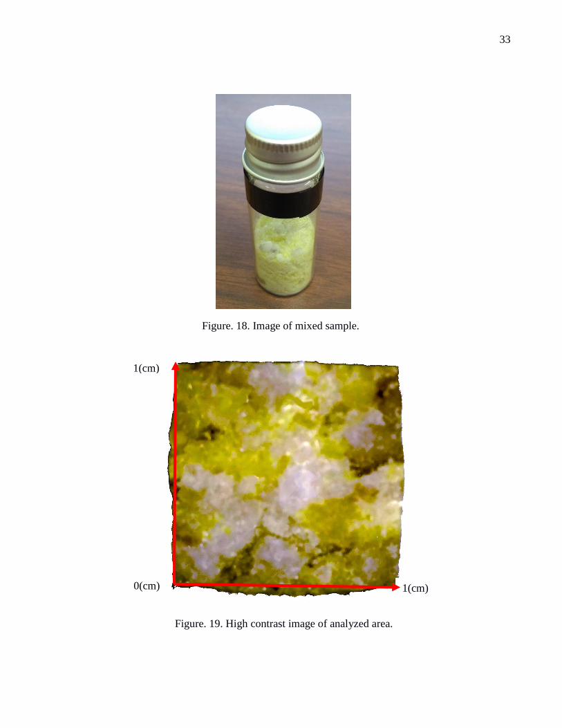
the strike point. A picture of the uncovered sample bottle can be seen in Figure. 18. A high contrast
image of the 1 cm2 sample window can be seen in Figure. 19.
33
0(cm) 1(cm)
1(cm)
Figure. 18. Image of mixed sample.
Figure. 19. High contrast image of analyzed area.

34
The model used to analyze this sample was trained with the 5-class dataset collected in NASA
LaRC’s Raman lab. The data points from this mixed sample were collected on the same 532 nm Raman
system described in Chapter 2. Despite the mixed sample only containing 2 of the 5-classes which are
in the dataset, the model was trained for all 5-classes to see if any false positives would be reported. As
shown in Figure. 20, the training time was rather quick, requiring just under 6 seconds for all 5 sub-
FNNs to be prepared. All 5 of the sub-FNNs exited training upon reaching Matlab’s default minimum
gradient and required no retries due to a validation stop. Default values were used for the minimum
gradient, minimum error, and validation check training hyperparameters.
Figure. 20. Console output for training of 5-class model. The commands display the system
date & time (Y, M, D, H, M, S) at the beginning and end of model training as well as the sub-
FFN training exit states.
Figure. 21. Average naphthalene signal from training dataset with marked region of interest
boundaries. The vertical lines show which regions of the line profile were found by the model to
contain spectral features.

35
Figures 21 and 22 show the average naphthalene and sulfur signals across the training dataset.
The vertical line surrounding individual peaks or groups of peaks are the boundaries of the regions of
interest found by the training program. The program found 8 regions of interest for classifying
naphthalene and 2 for classifying sulfur. Table 1 shows the mean, standard deviations, mean plus 3
standard deviations, and max activation values expressed by each sub-FNN when presented with a non-
member input. AOS for this experiment was set to be the largest of all these calculated values, 0.1203.
Class
Alabaster Ice Water Naphthalene Sulfur
μ 2.16E-06 5.29E-06 1.18E-06 9.27E-06 6.90E-04
σ 1.67E-05 7.56E-05 1.32E-05 8.92E-06 9.10E-03
μ+3σ 5.21E-05 2.32E-04 4.08E-05 3.60E-05 2.80E-02
max 2.87E-04 1.40E-03 1.65E-04 1.65E-04 1.20E-01
Table 1: Mean, standard deviation, 3 sigma, and max activation values for all non-member
observations of all sub-FNNs. Max value, used as AOS, is highlighted.
Figure. 22. Average sulfur signal from training dataset with marked region of interest
boundaries. The vertical lines show which regions of the line profile were found by the model to
contain spectral features.

36
Figure. 23 shows the front image of the mixed sample with a superimposed grid of color-coded
spots.10,15 Each spot on the image overlay represents the center of the laser strike-point for a single data
point. Between each exposure, the sample was carefully moved in steps of 1mm to ensure the mixture
was not disturbed, data points were collected from a total area of 1 cm2. The color of each spot
corresponds to the label(s) that the model applied to that data point. A red spot means features from
both naphthalene and sulfur had activations above the AOS, a yellow spot means only sulfur features
had activation above the AOS, and a green spot means only naphthalene features had activations above
the AOS.
Figure. 23. High contrast image of mixed naphthalene and sulfur. Red = mixed classification,
yellow = sulfur classification, green = naphthalene classification. A series of naphthalene and
mixed classifications can be seen to follow the while vein of naphthalene present from (1,1) to
(9,8).10,17

37
A series of mixed and naphthalene classifications can be seen to follow the white vein of
naphthalene as it extends diagonally upwards from data points (1,1) to (9,8). Due to how fine the sulfur
was ground a small amount of sulfur powder was covering all of the larger chunks of naphthalene,
which is not clearly visible in the high contrast sample image. The darker areas of the image
correspond with voids in the sample itself, where less material was pressed directly against the sample
bottle. No false alarms were reported for any of the non-present classes (alabaster, ice, and water).
5.3 Simulated mixed sample signals
Two simulations were conducted to test the model’s accuracy when passed inputs containing
spectral features of more than two samples and to verify pure sample classification accuracy matches
accuracies achieved by current models. In both simulations, completely random combinations of a set
amount of total classes were generated by adding average class signals together following Equation 5.3
where xs is the combined signal, a is a random value between [0.1, 1.0] rounded to the nearest tenth,
and xi is the average signal of a randomly selected sample class with intensity values scaled between 0
and 1.12,13 The total amount of class averages added together, N, is set by the user. Special care was
taken during coding to ensure no one class could be selected twice.
𝑥𝑠 = ∑ 𝑎𝑥𝑖
𝑁
𝑖=1
Two datasets were used to generate two different models. The first dataset consists of Raman
data from 5 different samples collected all on the same system in the Raman lab. The second dataset
consists of Raman data from 23 different materials and was generated by picking samples out of two
combined Raman databases which had at least 50 unique observations. Because the databases
maintained by the RRUFF project contain many data points taken on different systems, all Raman line
profiles were scaled to a single x-axis with a set dx of 0.5 (cm-1). The 23-class dataset was left balanced
(equal amount of training observations per class) to counteract the expected negative effect that x-axis
(5.3)
Fig.
3.
Timi
ng
profi
ler
outp
ut
from
5-
class
simul
ated
mixe
d
signa
ls.(4.
1)
Fig.

38
scaling would have on classification accuracy. The scaling process will be discussed in depth in Section
5.3.3.
Performance of the model in these experiments is quantified by calculating the probability of
detection (pd) and probability of false alarm (pfa) for any arbitrary component signal in xs. For both
datasets: all sub-FNNs in the model had 200 hidden units, the AOS was set to a constant value of 0.5,
1000 iterations were run for every N, and N was swept from 1 to the total amount of classes in the
dataset. For all iterations where N equaled 1, random noise was added along with the intensity scaling
to increase differences between the simulated signal and the training data. Information pertinent to both
model’s training processes will be provided in their respective sections. The results of each combined
pure signal experiment will show the pd and pfa values for all values of N and the prevalence of each
pure sample in all observations where the model failed to detect at least one component signal.
Comments will be made on any visible trends in the failed observations.
5.3.1 Traditional Matched Filter
The combined “excellent oriented” and “excellent unoriented” databases maintained by the
RRUFF project contains Raman spectra from over 1600 minerals. For this experiment, mineral classes
with at least 50 observations were selected and a balanced dataset was created from these data points.
In total, this dataset contains 1150 unique data points from 23 total classes. The dataset was left
balanced to help counteract the expected loss of accuracy from x-axis scaling. Data point scaling was
accomplished by creating a new x axis ranging from 0 to 1577 cm-1 with a constant dx and extracting
intensity values associated with the closest x value on the unscaled data point’s x axis. Any leading or
trailing zeros were replaced with random noise to prevent zero variance errors from occurring during
training, no other modifications were made to the data points from the RRUFF databases. The feature

39
selection functionality of the presented model was implemented in this matched filter implementation
by the same methodology to allow for a more direct comparison between the two models performances.
Figure. 24. shows the probability of detection (Pd) and probability of false alarm (Pfa) of an
arbitrary signal being detected as a function of the amount of total materials in the randomly combined
input (N). As expected, Pd decreases with the number of total signals in an input. It can be seen that the
probability of detection rapidly decays as the N increases. Also, the probability of false alarm is
unacceptably high in the cases of N equaling 1 through 8, reaching far above 90% in the N equals 1
case. Although this model is capable of detecting multiple Raman signatures in a single input, the high
probability of false alarm poses too much of a risk to use matched filters even as a pure signal
classifier.
Figure. 24. Pd and Pfa values plotted for all values of N in mixed pure sample signals experiment
using 23 class data set from RRUFF databases and the matched filter model10. Pd decays faster
than the presented model, and Pfa is far higher than that of the presented model for the N equals
1 through 7 cases.

40
5.3.2 5-Class dataset
The 5-material dataset consists of Raman spectra from alabaster, water, ice, naphthalene, and
sulfur. All data points in this dataset were collected on the same Raman system in the LaRC Raman
spectroscopy lab, and the training dataset for the naphthalene and sulfur mixed sample experiment was
derived from this dataset. The entire dataset was used for training and the AOS was set at a constant
value of 0.5.
Compared to the naphthalene and sulfur real mixed sample experiment, which used exactly half
of this dataset for training, total training time increased by 28% to 8.376 seconds. All sub-FNNs exited
their individual training by reaching minimum gradient. Total simulation time for all 1000 signals for
all 5 Ns took about 26 minutes, timing profiler output can be seen in Figure 25.
The analysis of the 5000 simulated signals took a total of 1605s, excluding generation. This
results in an average analysis time of 0.3s per signal. Generation of the simulated mixed signals
accounted for less than 1% total execution time.
Figure. 25. Timing profiler output from 5-class simulated mixed signals
Fig. 27. Probability of detection (pd) plotted versus N with a line of best fit
projecting pd for higher N values.Fig. 25. Timing profiler output from 5-class
simulated mixed signals

41
N Probability of Detection (pd)
Probability of False Alarm (pfa)
1 1 0
2 0.9930 0
3 0.9590 0
4 0.8548 0
5 0.7130 0
Table 2: Probability of detection and probability of false alarm (pd and pfa) for all Ns in 5-class
simulation.
Fig. 11. Calcite Raman spectra from two different systems. Although both data points are correctly
calibrated, scaling is required before use with the model due to the differing x-axis, total length, and
range of shift.Table 3: Probability of detection and probability of false alarm (pd and pfa) for all Ns in
Figure. 27. Probability of detection (pd) plotted versus N with a line of best fit projecting pd for higher
N values.
Figure. 26. Composition of observations with at least one undetected component for all
N in 5 class simulation. Legend labels are associated with bars left to right.

42
Figure. 26. shows what percentage of observations with at least one undetected component
contained each pure sample signal for all values of N. For all 1000 iterations where N equaled 1, there
were no misclassifications. In the cases where N equaled 2 and 3, it can be seen that observations
containing both water and ice component signals were more likely to be misclassified. This is likely
due to the similarities between water and ice Raman signatures. It can also be seen that as N increases
the composition of misclassified signals begins to even out, this is indicative of the complexity of the
signal becoming the limitation in pd instead of similarities between component signals. Because all
generated signals contained all pure signals when N equaled 5, the complexity of the generated signal
was the only possible cause of a failed classification.
Figure. 27. shows pd plotted versus N along with a calculated line of best fit. The trend in this 5-
iteration case shows pd decaying rather rapidly as N increases, however, as will be seen in the RRUFF
23 dataset results section, non-zero pd has been recorded with as high as 23 component signals.
5.3.3 Preparation of spectra from RRUFF datasets
Due to the Raman data in the RRUFF project’s datasets being collected on different systems, x-
axis scaling needed to be performed for compatibility with the presented model. Figure. 28. highlights
the issues which needed to be solved before use. Subplots A and B show two different calcite Raman
spectra data points from the RRUFF project’s “excellent oriented” database before scaling. The 155,
281, 711, 1085, and 1434 cm-1 Raman peaks can be seen in both. Neither system was able to detect the
1748 cm-1 Raman peak. This could be due to the sensors not being large enough to detect diffracted
light of that wavelength or the spectrometers diffractive optic not functioning at that wavelength at all.
Although both data points were calibrated well on their own systems, x-axis scaling needs to be
performed to correct the mismatching input lengths, standardize the total range of Raman shift covered
in the line profile, and correct unequal spectral resolutions.

43
Line profile scaling was performed by creating a new Raman shift (x) axis for all data points to
follow and assigning intensity (y) values from the source line profile for each point on the new x-axis.
The new Raman shift axis ranges from 0 to 1577 cm-1, based off of the longest shift detected in a data
point, and has a constant dx of 0.5 cm-1 for a total input length of 3155 units. Any leading or trailing
zeros left over in the scaled data point were replaced with random values between 0 and 1 to prevent
zero variance cases from occurring during model generation. In cases where the source line profile had
a higher spectral resolution than the new x-axis (a dx less than 0.5 cm-1) some data was lost in the
scaling process. This loss of data could lead to an increased probability of false alarm and a decreased
probability of detection. Figure. 29. A and B show the same calcite data points after they had been
scaled to the same Raman shift axis. Peak positions are calibrated to the closest 0.5 cm-1 from their
original positions and the overall length of the line profiles is now the same.
Figure. 28. Calcite Raman spectra from two different systems. Although both data points are correctly
calibrated, scaling is required before use with the model due to the differing x-axis, total length, and
range of shift.
A
A
A
A
A
A
A
A
B
Fi
g.
2
0.
C
al
ci
te
R
a
m
a
n
sp
ec
tr
a
fr
o
m
t
w
o
di
ff
er
e
nt
sy
st
e
m
s
a
p
pl
ie
d
to
a

44
5.3.4 23-Class dataset
This 23 class simulation uses the same dataset that was used to test the traditional matched
filter. Training of the 23-class model for this experiment took just over 2 minutes. All sub-FNNs exited
training by reaching minimum gradient. Total simulation time for 1000 data points over 23 values of N
took 11 hours and 9 minutes, a screenshot of the timing profiler can be found in Figure 30. Figure 31
shows pd and pfa plotted versus N along with a calculated line of best fit.10 The trend in this 23 iteration
case shows pd decaying rather rapidly as N increases, however, the rate of decay in pd decreases as N
increases, appearing to reach an asymptotic minimum at 14%. The pfa appears to have no rate of growth
or decay with a max value of 0.037167 at N = 6. The false alarms could be caused by similarities
between the Raman spectra of different classes and by the use of a scaled x-axis as the scaling process
did lead to a loss of information in data points which had a smaller dx than 0.5 (cm-1).
A
Fi
g.
2
1.
Ti
m
in
g
pr
of
il
er
o
ut
p
ut
fr
o
m
2
3
cl
as
s
si
m
ul
at
e
d
m
ix
e
d
si
g
n
al
s.
A
Fi
g.
2
1.
Ti
m
in
g
pr
B
B
B
B
B
B
B
B
Figure. 29. Calcite Raman spectra from two different systems applied to a new Raman shift axis. The
peak positions are still properly calibrated and the overall length of both data points are the same.

45
Figure. 30. Matlab timing profiler output from 23 class simulated mixed signals. Entire run took 11
hours and 9 minutes averaging 1.7 s to analyze a single line profile.
Figure. 31. pd and pfa values plotted for all values of N in mixed pure sample signals experiment
using 23 class data set from RRUFF databases.10

46
Figure. 32. Composition of observations with at least one undetected component for all N in 23
class simulation. Top to bottom of legend labels follow bars left to right.

47
Figure. 32. shows what percentage of observations with at least one undetected component
contained each pure sample signal for all values of N. For all 1000 iterations where N equaled 1, there
were no misclassifications. In the N = 2, 3, and 4 cases, it can be seen that some component signals are
in significantly more misclassified observations than other. This is possibly due to the use of a scaled x-
axis and the varying spectral resolutions which are seen in this dataset. It can also be seen that as N
increases the composition of misclassified signals begins to become more consistent, however, some
samples are still significantly more common in misclassifications than others. For example, when N =
21 Albite was about 7% more common in misclassifications than Titanite.

48
CHAPTER 6
DISCUSSION
This chapter summarizes the development of the Raman systems and the improved matched
filter model. Results from model validation and future work which could increase spectrometer
performance and model accuracy will be discussed.
In this thesis, an improved matched filter model for classification of Raman spectra and two
Raman spectrometer systems were developed and tested. The 532nm gated system was designed to use
a high-powered laser at a reasonable sample distance suitable for lab use. The system used an off-the-
shelf camera and spectrometer housing. The spectrometer was equipped with a custom, two region
VPH grating make by Kaiser Optical Systems for high diffraction efficiencies up to 4500 cm-1 of
Raman shift. The spectrometer was equipped with high optical density Semrock long pass filter
allowing the system to detect shift as low as 80 cm-1. The transmitting optics utilized a prism allowing
the laser to be used at full power and coaxial geometry for optimal backscatter collection.
The receiving optics utilized a 2” diameter collection lens to collect more backscattered light
and a 20x microscope objective was used to focus light into the spectrometer for optimal collimation in
its filtering section. The ICCD camera was equipped with a gated intensifier, experiments were run in
gated mode to optimize signal to noise ratio and to allow for more comfortable operational conditions
with the room lights on. In the past, this laser and spectrometer have not been able to receive Raman
signal at samples distances this short. The 532 nm system performed well with mineral and liquid
samples, however, there was high levels of laser induced fluorescence when biological samples were
used. Performance of this system could be improved by reducing the size of the telescope section of the
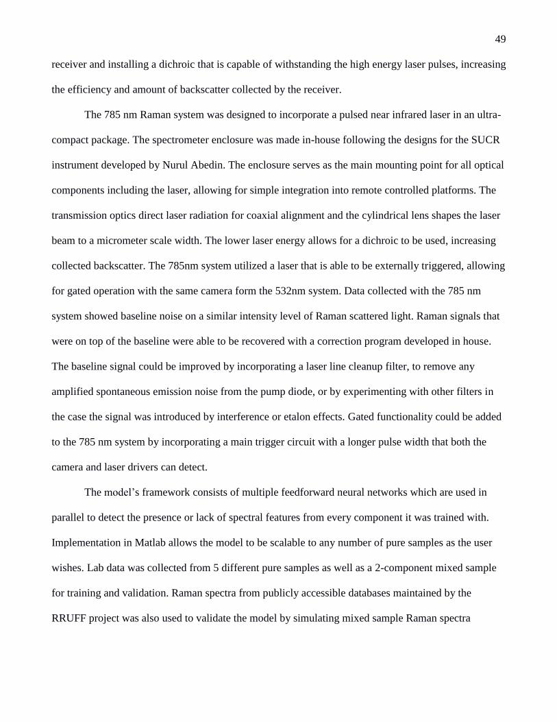
49
receiver and installing a dichroic that is capable of withstanding the high energy laser pulses, increasing
the efficiency and amount of backscatter collected by the receiver.
The 785 nm Raman system was designed to incorporate a pulsed near infrared laser in an ultra-
compact package. The spectrometer enclosure was made in-house following the designs for the SUCR
instrument developed by Nurul Abedin. The enclosure serves as the main mounting point for all optical
components including the laser, allowing for simple integration into remote controlled platforms. The
transmission optics direct laser radiation for coaxial alignment and the cylindrical lens shapes the laser
beam to a micrometer scale width. The lower laser energy allows for a dichroic to be used, increasing
collected backscatter. The 785nm system utilized a laser that is able to be externally triggered, allowing
for gated operation with the same camera form the 532nm system. Data collected with the 785 nm
system showed baseline noise on a similar intensity level of Raman scattered light. Raman signals that
were on top of the baseline were able to be recovered with a correction program developed in house.
The baseline signal could be improved by incorporating a laser line cleanup filter, to remove any
amplified spontaneous emission noise from the pump diode, or by experimenting with other filters in
the case the signal was introduced by interference or etalon effects. Gated functionality could be added
to the 785 nm system by incorporating a main trigger circuit with a longer pulse width that both the
camera and laser drivers can detect.
The model’s framework consists of multiple feedforward neural networks which are used in
parallel to detect the presence or lack of spectral features from every component it was trained with.
Implementation in Matlab allows the model to be scalable to any number of pure samples as the user
wishes. Lab data was collected from 5 different pure samples as well as a 2-component mixed sample
for training and validation. Raman spectra from publicly accessible databases maintained by the
RRUFF project was also used to validate the model by simulating mixed sample Raman spectra

50
containing spectral features from up to 23 different materials. The model, analysis, and simulation
programs were written in Matlab R2018a.
A feature selection subroutine was built into the model’s training program which only passes
pertinent data forward to each sub-FNN, decreasing computational load of running multiple FNNs in
parallel and the chances of a false positive from noise or non-important spectral features which may be
present in other areas of the line profile.
Analysis of an arbitrary input signal is accomplished by iteratively forward propagating sections
of a line profile through each sub-FNN. The areas of the line profile that are analyzed correspond to the
regions of interest of each sub-FNN that were found during training. The model’s output consists of a
1-dimensional matrix of activation values from each sub-FNN in the order that they were trained. A
positive detection for an arbitrary class is labeled as such by comparing the class’ respective sub-
FNN’s activation to a user-set minimum. In this thesis the minimum activation value was calculated
using equation 4.9. Each simulated signal was only analyzed once for both the 5 and 23 class datasets.
Model validation was accomplished by analyzing real and simulated Raman signals which
contained spectral features from multiple pure samples. The real mixed sample data was collected from
a mixture of naphthalene and sulfur. The classifications assigned by the model agreed with analysis
done by visual inspection of the Raman line profiles. No false alarms for known non-present materials
were reported.
Simulated mixed sample line profiles were generated by randomly combining class Raman
signals.12,13 Two different datasets were used, the first was collected on a time gated Raman
spectrometer built at NASA LaRC, the second was a combination of two publicly accessible databases
maintained by the RRUFF project. Analysis of the real mixed sample data as well as the simulated
mixed sample data showed that this model can detect multiple materials in a single line profile.

51
The simulated mixed sample performance showed that the model is capable of pure sample
classification and can have non-zero probability of detection for signals containing as many as 23
different components. The simulation results also show that this model is not adversely affected by max
intensities of an input signal deviating from those of the training dataset. When a traditional matched
filter was tested with scaled inputs, classification failures were more common. By effectively using
FNNs as class filters, this model was able to learn the important relative intensities of spectral
features while placing no observed importance on overall signal intensity.
The model was developed into a custom scan analysis program that was designed for direct
compatibility with the SUCR instrument developed by Dr. Nurul Abedin.2 Figure. 33. shows the
finalized analysis program window. When the number of classes present in a simulated signal are low,
large differences in the composition of the misclassified signals can be seen. For example, when N
Figure. 33. Custom scan analysis program window. Whole scans collected by the SUCR system can
be analyzed automatically.

52
equaled 2 in the 5-class simulation, 100% of all signals with at least one failed classification contained
both water and ice signals. Similar discrepancies were seen in the 23-class simulation, however, none
were as extreme as the N = 2 run of the 5 class simulation. In both simulations, the composition of
misclassified signals becomes more consistent as N increases. Both the 5 class and 23 class simulations
show the probability of detection dropping off quickly as the number of classes in a simulated signal
increase. This is likely due to distinct spectral features being “hidden” by combinations of other
spectral features. The 23-class simulation shows that the decay rate of pd slows as N continues to
increase and never actually reaches zero.
Due to Raman spectra of mixed samples being a combination of the pure sample line profiles,
probability of detection could be increased by changing the analysis procedure. Incorporating code that
will subtract away spectral features of classes that reached the AOS and re-analyze the signal for any
classes not found in the first run and repeating until no more materials are found could allow for classes
with lower relative intensity to be detected as long as matrix effects are not a factor in the detected
signal.
A change in model architecture entirely could also allow for higher probability of detection and
eliminate the need for OVA decomposition and feature selection as seen in this thesis. The recently
developed “capsule net” is able to outperform CNN in image classification tasks and is capable of
multi-label classification.37 Capsule net also greatly outperforms CNN when classifying highly
overlapping image features. Although capsule net’s focus is image processing, the capabilities of
capsules make good performance likely on 1 dimensional data. Other multi-label capable models are
also available for simple implementation using Matlab or Python and scikit-learn.7

53
CHAPTER 7
CONCLUSIONS
This thesis presented an improved matched filter model for classification of Raman spectra and
two Raman spectrometer systems. The two spectrometers were able to detect Raman scattered light and
the model showed improved probabilities of detection for mixed sample signals and much reduced
probabilities of false alarm.
The 532 nm system was able to controllably use a high energy pulsed laser at sample distances
convenient for lab use. The gated functionality of the ICCD camera enabled the system to operate with
in ambient room light and improved signal to noise ratio. High quality mineral and liquid sample
Raman data was able to be collected. The 785 nm system is equipped with a lower energy laser,
reducing the effect of laser induced fluorescence. The ultra-compact enclosure also enables the system
to be easily incorporated into a mobile platform. Improvements to the 785nm system can be made by
adding a longer pulsed timing circuit to serve as the main trigger and a laser cleanup filter.
The model was tested with data from publicly accessible databases as well as from the 532 nm
system. Real and simulated mixed sample Raman data was analyzed using the presented model. Mixed
sample classification was achievable on all datasets that were tested, and non-zero detection
probabilities were seen on simulated signals with as many as 23 components.
Although the presented model is capable of detecting multiple samples a single line profile, the
probability of an arbitrary component’s Raman signal being detected decreases as the amount of
present signal components increases. This model is also prone to issues in classification of Raman
signals which have large amounts of overlap between each other, such as water and ice. Future research

54
into model improvements and architecture changes can increase classification accuracy and decrease
computational load of training and analysis.

55
REFERENCES
1. E. Efremov, F. Ariese and C. Gooijer, "Achievements in resonance Raman spectroscopy
Review of a technique with a distinct analytical chemistry potential", Analytica Chimica Acta,
vol. 606, pp. 119-134, 2007.
2. M.N. Abedin, A. Bradley, A. Misra, Y. Bai, G. Hines and S. Sharma, "Standoff ultracompact
micro-Raman sensor for planetary surface explorations", Applied Optics, vol. 57, no. 1, p. 62,
2017.
3. J. Lin, R. Chen, S. Feng, J. Pan, B. Li, G. Chen, S. Lin, C. Li, L. Sun, Z. Huang and H. Zeng,
"Surface-enhanced Raman scattering spectroscopy for potential noninvasive nasopharyngeal
cancer detection", Journal of Raman Spectroscopy, vol. 43, no. 4, pp. 497-502, 2011.
4. J. Martinez, J. Guzmán-Sepúlveda, G. Bolañoz Evia, T. Córdova and R. Guzmán-Cabrera,
"Enhanced Quality Control in Pharmaceutical Applications by Combining Raman Spectroscopy
and Machine Learning Techniques", International Journal of Thermophysics, vol. 39, no. 6,
2018.
5. J. Liu, M. Osadchy, L. Ashton, M. Foster, C. Solomon and S. Gibson, "Deep convolutional
neural networks for Raman spectrum recognition: a unified solution", The Analyst, vol. 142, no.
21, pp. 4067-4074, 2017.
6. S. Khan, R. Ullah, S. Shahzad, N. Anbreen, M. Bilal and A. Khan, "Analysis of tuberculosis
disease through Raman spectroscopy and machine learning", Photodiagnosis and
Photodynamic Therapy, vol. 24, pp. 286-291, 2018.
7. 1.12. Multiclass and multilabel algorithms — scikit-learn 0.20.0 documentation", Scikit-
learn.org, 2018. [Online]. Available: https://scikit-learn.org/stable/modules/multiclass.html.
[Accessed: 14- Nov- 2018].
8. Raman Spectrosopy Basics, 2018. [Online]. Available:
http://web.pdx.edu/~larosaa/Applied_Optics_464564/Projects_Optics/Raman_Spectrocopy/Ra
man_Spectroscopy_Basics_PRINCETON-INSTRUMENTS.pdf. [Accessed: 14- Nov- 2018].
9. J. Ferraro, K. Nakamoto and C. Brown, Introductory Raman spectroscopy. Amsterdam:
Academic Press, 2003.
10. A. Atkinson, M.N. Abedin, G.D. Hines, A.T. Bradley, H. Elsayed-Ali, Machine Classification
of Raman Spectra Using Feedforward Neural Networks for In Situ Life Detection Missions.
Poster session presented at: Astrobiological Science Conference (AbSciCon), 2019 Jun 24-28,
Bellevue, WA

56
11. S. Chatterjee, "Capsule Networks and the Limitations of CNNs - Saama Technologies", Saama
Technologies, 2018. [Online]. Available: https://www.saama.com/blog/capsule-networks-
limitations-cnns/.
12. "Quantifying mineral abundances in mixtures using raman spectroscopy: calculating raman
coefficients using a diamond reference.", 47th Lunar and Planetary Science Conference, p.
2186, 2016. Available: https://www.hou.usra.edu/meetings/lpsc2016/pdf/2186.pdf. [Accessed
22 September 2019].
13. S. Sharma, A. Misra, S. Ismail and U. Singh, "Remote raman spectroscopy of various mixed
and composite mineral phases at 7.2 m distance.", Lunar and Planetary Science XXXVII, p.
Paper 2285, 2006. Available:
https://www.researchgate.net/publication/252521525_Remote_Raman_Spectroscopy_of_Vario
us_Mixed_and_Composite_Mineral_Phases_at_72_m_Distance. [Accessed 22 September
2019].
14. "Database of Raman spectroscopy, X-ray diffraction and chemistry of minerals", Rruff.info,
2018. [Online]. Available: http://rruff.info/about/about_general.php. [Accessed: 18- Dec-
2018].
15. C. Bishop, Pattern Recognition and Machine Learning, 1st ed. New York, NY: Springer
Science + Business Media, LLC.
16. M. Matsugu, K. Mori, Y. Mitari and Y. Kaneda, "Subject independent facial expression
recognitionwith robust face detection using a convolutional neural network", Neural Networks,
vol. 16, no. 5-6,pp. 555-559, 2003.
17. A. Atkinson, M.N. Abedin, G.D. Hines, A.T. Bradley, H. Elsayed-Ali, Automated Analysis of
Mixed Sample Raman Spectra Using Feedforward Neural Networks and One-VS-All
Decomposition. Poster session presented at: Old Dominion University Graduate Research
Appreciation Day (GRAD), 2019 Mar 28, Norfolk, VA.
18. "Signal Detection in White Gaussian Noise- MATLAB & Simulink", Mathworks.com, 2019.
[Online]. Available: https://www.mathworks.com/help/phased/examples/signal-detection-in-
white-gaussian-noise.html. [Accessed: 10- Sep- 2019].
19. "User’s Manual ULTRA CFR Nd:YAG Laser System", www.Bigskylaser.com, 2004. [Online].
Available: http://ftp://ftp.lanl.gov/public/sclarke/Murphy-
June07/BIG%20SKY%20PIV%20LASER%20Manuel/ULTRA.pdf. [Accessed: 13- Dec-
2018].
20. "HoloSpec Imaging Spectrograph OPERATIONS MANUAL", www.Kosi.com, 2002.
[Online].Available:https://psfcsv10.psfc.mit.edu/~rowan/page4/page6/assets/HoloSpec_V2.pdf.
[Accessed: 13- Dec- 2018].

57
21. "PI-MAX/PI-MAX2 System Manual", www.princetoninstruments.com/, 2011. [Online].
Available: http://www.pi-j.jp/pdf/manual/PI-MAX_SystemManual.pdf. [Accessed: 13- Dec-
2018].
22. D. Paschotta, "Encyclopedia of Laser Physics and Technology - Q switching, Q-switched laser,
pulses, modulator, saturable absorber, self Q switching", Rp-photonics.com, 2018. [Online].
Available: https://www.rp-photonics.com/q_switching.html. [Accessed: 18- Dec- 2018].
23. "KTP Data Sheet", Northropgrumman.com, 2018. [Online]. Available:
http://www.northropgrumman.com/BusinessVentures/SYNOPTICS/Products/SpecialtyCrystals
/Documents/pageDocs/KTP_data_sheet.pdf. [Accessed: 18- Dec- 2018].
24. T. Erdogan, Optical Filters Filters for Raman & Laser Applications. Semrock, A Unit of IDEX
Corporation, 2018.
25. "Intro to VPH for Transmission | Kaiser Optical Systems, Inc. | An Endress+Hauser Company",
Kosi.com, 2018. [Online]. Available: http://www.kosi.com/na_en/products/holographic-
gratings/vph/intro-to-vph-for-transmission.php. [Accessed: 20- Dec- 2018].
26. "Resolution of Monochromators and Spectrographs", Newport.com, 2018. [Online]. Available:
https://www.newport.com/t/resolution-of-monochromators-and-spectrographs. [Accessed: 20-
Dec- 2018].
27. Hamamatsu.com. (2014). Gated ICCD Camera Series - Ideal for imaging extreme low light fast
phenomena!. [online] Available at:
https://www.hamamatsu.com/resources/pdf/sys/SHSS0018E_C11370.pdf [Accessed 21 Dec.
2018].
28. "The Technology Behind ICCD Cameras | Andor", Andor.com, 2018. [Online]. Available:
http://www.andor.com/learning-academy/intensified-ccd-cameras-the-technology-behind-iccds.
[Accessed: 21-Dec-2018].
29. C. Garcia, N. Abedin, S. Ismail, S. Sharma, A. Misra and H. Elsayed-Ali, "Studies of minerals,
organic and biogenic materials through time resolved Raman spectroscopy", SPIE Digital Library,
2009. Available: https://doi.org/10.1117/12.818169 [Accessed 14 June 2019].
30. "CrystaLaser Product Catalog", Crystalaser.com, 2019. [Online]. Available:
http://www.crystalaser.com/home.htm. [Accessed: 08- Sep- 2019].
31. "Semrock - Part Number: LPD02-785RU", Semrock.com, 2019. [Online]. Available:
https://www.semrock.com/FilterDetails.aspx?id=LPD02-785RU-25. [Accessed: 08- Sep- 2019].
32. "wasatch photonics vph gratings", Google.com, 2019. [Online]. Available:
https://wasatchphotonics.com/product-category/gratings-and-diffractive-optics/. [Accessed: 08-
Sep- 2019].

58
33. "7 Types of Neural Network Activation Functions: How to Choose? - MissingLink.ai",
MissingLink.ai, 2019. [Online]. Available: https://missinglink.ai/guides/neural-network-
concepts/7-types-neural-network-activation-functions-right/. [Accessed: 28- Jul- 2019].
34. H. Yu and B. Wilamowski, "Levenberg–Marquardt Training", Eng.auburn.edu, 2010. [Online].
Available: http://www.eng.auburn.edu/~wilambm/pap/2011/K10149_C012.pdf. [Accessed: 25-
Dec- 2018].
35. H C Eilers, Paul & F M Boelens, Hans. (2005). Baseline Correction with Asymmetric Least
Squares Smoothing. Unpubl. Manuscr. [online] Available
https://zanran_storage.s3.amazonaws.com/www.science.uva.nl/ContentPages/443199618.pdf
36. P. Eilers, "A Perfect Smoother", Analytical Chemistry, vol. 75, no. 14, pp. 3631-3636, 2003.
Available: 10.1021/ac034173t.
37. G. Hinton, S. Sabour and N. Frosst, "Dynamic Routing Between Capsules", Papers.nips.cc, 2017.
[Online]. Available: https://papers.nips.cc/paper/6975-dynamic-routing-between-capsules.pdf.
[Accessed: 28- May- 2019].

59
APPENDIX A
FEATURE SELECTION FOR MODEL TRAINING
A.1. Necessity of feature selection
It was found early on in this model’s development that utilizing the entire Raman line profile
for training and using only a single feedforward neural network for classification were not going to be
possible when training with pure sample data only. Due to the need for one vs all decomposition, there
will be high computational load during training and analysis if the full line profile is used as the input
for every FNN that is in a trained model. To make training and analysis faster, code that locates the
spectral features of each class and limits the input of each sub-FNN to those areas of the line profile
was incorporated into the training program.
A.2. Feature selection methodology
Feature selection was accomplished by calculating mean and standard deviation of the average
class line profile twice, once with all intensity values included in the calculation and a second time
ignoring spectral data which rises above the first calculated mean plus a user set amount of first standard
deviations. The data used in this thesis was able to work well with only 1 standard deviation, however,
the optimal amount to add will change from one system to another. The second recalculation of the mean
and standard deviation was found to be necessary to include dimmer spectral details and retain
compatibility with broader Raman features such as those of ice and water. This process is visualized in
Figure A1, the Sulfur Raman signal is shown with the first and second calculations of the signal mean
plus one standard deviation (red and green lines respectively). The moment a signal rises above 2 + 2
the model traces the signal to the left and right until it falls below 2 again, this range of values on the
line profile is called a “region of interest” (ROI) and is one of the areas of the line profile a sub-FNN will

60
analyze. As can be seen, dimmer spectral features may be missed if the first mean and standard deviation
are used to define the ROIs. Due to this nature of zone definition, it is possible for multiple spectral
features to be in a single ROI. It is also possible for two ROIs to share a beginning and end point due to
how the code was written, this was not found to cause any issues during model validation.
Figure A1: Region definition by double calculation of signal mean and standard deviation. Regions 1-4
are defined by where the line profile rises above the second mean and standard deviation.
ROIs for signals with no broad features were also able to be found by analyzing the “first
derivative” of the line profile. Figure A2 shows an Auger plot of a sulfur Raman line profile calculated
by finite difference. The spectral peaks have been replaced with sharp peaks immediately followed by
sharp troughs, corresponding to the positive and negative slopes on each side of a Raman peak. ROIs
could also be found by monitoring deviations from zero, as the first derivative is likely to have a mean
very close to zero. Issues were found, however, when this method was applied to materials with wide
Raman peaks, such as ice and water. The broad features have “flat” areas around their center, making

61
the first derivative close enough to zero for the program to think the feature had ended, as seen in
Figure A3.
Figure A2: First derivative of sulfur Raman line profile.
Figure A3: Raman line profile of water and its first derivative. The values holding close to zero would
cause the program to think the spectral feature had ended.

62
APPENDIX B
CLASSIFYING RAMAN DATA WITH FEEDFORWARD NEURAL NETWORKS
B.1. Formatting data for training and analysis
Matlab implementation of this model made use of the built-in libraries and shallow neural
network training tool for the training of each sub-FNN. With this being the case, the format by which
Raman data is passed to either the training or analysis programs was designed to be consistent with
Matlab functions from the neural network and deep learning toolboxes.
A single training or analysis data point consists of a 1-dimensional matrix of the intensity
values from a Raman line profile. This implementation assumes that the x-axis is the same across all
the data points it sees, whether its units are pixels or nanometers or Raman shift is unimportant.
The model training program needs two matrices to begin training. The first, which will be
referred to as “X”, is the training dataset and contains all full-length Raman line profiles that will be
used in model generation. X will have the dimensions of [O-by-F] where O is the number of
observations (or individual data points) in the training dataset and F is the number of features (or
pixels) that are in a single data point. One row of X represents a single line profile. The second matrix
needed by the training program, referred to as “Y”, contains the class labels of the training
observations. Y will have the dimensions of [O-by-C] where O is the number of observations (Y must
have the same number of rows as X) and C is the class that an observation belongs to. Due to each
training observation only belonging to one class, Y will be a sparse matrix. Each row of Y will have
zeros for all columns except for the class that the observation belongs to which will have a 1.
A softmax layer cannot be used as the output layer’s activation function because the sub-FNN
output is a single neuron. Sigmoid was used in this model instead. Matlab should automatically set the

63
output layer activation function to sigmoid (Matlab calls it “logsig”) when it sees that the FNN was
initialized with only one output neuron.
B.2. How feedforward neural network outputs are calculated
Figure B1 shows the structure of a 3-layer feedforward neural network. Each circle represents a
neuron and each line between neurons represents a learned weight. Each neuron in the FNN has a
transfer function and bias associated with it. All together the FNN structure represents a series of
equations which will calculate a value at the network’s output.
When the FNN is initialized, all weights and biases are typically random values. By training the
neural network, ideal weights can be found which minimizes the output’s overall error. Training is
Figure B1: Feedforward neural network structure with an input length of 5, 3 hidden units, and
1 output neuron.

64
accomplished by minimizing an error function via gradient descent with respect to every weight in the
FNN, mean squared error was used as the error function for all sub-FNN training in this thesis.
Output values are calculated by forward propagating an input through the network. All values in
the input layer are first passed to the hidden layer. Each hidden unit performs a dot product with the
input values and its learned weights, adds its random bias, and applies its transfer function. If, for
example, the hidden layer’s activation function was hyperbolic tangent. Each hidden unit “i" would
calculate its value using
ℎ𝑖 = tanh ((𝑥 ∙ 𝜔𝑖) + 𝑏𝑖)
The output layer would then calculate its value(s) following a similar process. For each neuron
“j” in the output layer, the hidden unit values would be dotted with the output neuron’s learned
weights, its bias would be added, and its transfer function would be applied. If, for example, the output
layer’s transfer function was sigmoid, the output values would be calculated using
𝑂𝑗 = 𝜎((ℎ ∙ 𝜔𝑗) + 𝑏𝑗)
Where
𝑠𝑖𝑔𝑚𝑜𝑖𝑑(𝑛) = 𝜎(𝑛) = 1
1 + 𝑒−𝑛
(B1)
(B2)
(B3)

65
VITA
NAME:
DATE OF BIRTH:
EDUCATION:
Master of Science, Electrical and Computer Engineering, Old Dominion University
Norfolk, Virginia, 2017-Present
Bachelor of Science, Electrical Engineering, Old Dominion University, Honors College
Norfolk, Virginia, 2013-2017
EXPERIENCE:
Old Dominion University, Norfolk, VA
Undergraduate Student Researcher
Huntington Ingalls Industries, Newport News, VA
Electrical Engineering Intern
NASA LaRC, Hampton, VA
Graduate Research Assistant
NAVSEA, Virginia Beach, VA
Electrical Engineer
HONORS, AWARDS, AND MEMBERSHIPS:
ODU Honors College – December 2018 Graduate
Monarch Excellence Scholarship – Recipient
ASHRAE Student Chapter Gordon Webster Zipper Scholarship – Recipient
ODU Honors College Summer Research Grant, 2015 – Recipient
Kappa Sigma Fraternity, Sigma Theta Chapter – Alumni
January 2015 – April 2017
Summer 2016
May 2017 – June 2019
July 2019 – Present
Alexander Matthew Atkinson
October 1st, 1994