OPEN ACCESS

Demonstration of the temporal matter-wave Talboteffect for trapped matter wavesTo cite this article: Manfred J Mark et al 2011 New J. Phys. 13 085008

 

View the article online for updates and enhancements.

You may also likeNonlinear Talbot Effect and ItsApplicationsZhening Yang

-

Talbot effect for gratings with diagonalsymmetryJakub Blín and Tomáš Tyc

-

Observation of the Talbot carpet for waveson the liquid surfacA N Morozov, I V Moskvina, B G Skuibin etal.

-

Recent citationsSingle- to many-body crossover of aquantum carpetMaciej ebek et al

-

Fermionic quantum carpets: From canalsand ridges to solitonlike structuresPiotr T. Grochowski et al

-

Effects of finite momentum width on thereversal dynamics in a BEC based atomoptics -kicked rotorJay Mangaonkar et al

-

This content was downloaded from IP address 45.160.136.215 on 22/11/2021 at 04:21

T h e o p e n – a c c e s s j o u r n a l f o r p h y s i c s

New Journal of Physics

Demonstration of the temporal matter-wave Talboteffect for trapped matter waves

Manfred J Mark1, Elmar Haller1, Johann G Danzl1,Katharina Lauber1, Mattias Gustavsson2 andHanns-Christoph Nägerl1,3

1 Institut für Experimentalphysik und Zentrum für Quantenphysik,Universität Innsbruck, Technikerstraße 25, A-6020 Innsbruck, Austria2 Department of Physics, Yale University, PO Box 208120, New Haven,CT 06520, USAE-mail: Christoph.Naegerl@uibk.ac.at

New Journal of Physics 13 (2011) 085008 (15pp)Received 30 April 2011Published 10 August 2011Online at http://www.njp.org/doi:10.1088/1367-2630/13/8/085008

Abstract. We demonstrate the temporal Talbot effect for trapped matter wavesusing ultracold atoms in an optical lattice. We investigate the phase evolutionof an array of essentially non-interacting matter waves and observe matter-wave collapse and revival in the form of a Talbot interference pattern. By usinglong expansion times, we image momentum space with sub-recoil resolution,allowing us to observe fractional Talbot fringes up to tenth order.

Contents

1. Introduction 22. Preparation of the initial sample 33. Phase evolution and the Talbot effect 44. Experimental realization 65. Conclusion 11Acknowledgments 14References 14

3 Author to whom any correspondence should be addressed.

New Journal of Physics 13 (2011) 0850081367-2630/11/085008+15$33.00 © IOP Publishing Ltd and Deutsche Physikalische Gesellschaft

2

1. Introduction

Interference of matter waves is one of the basic ingredients of modern quantum physics. Ithas proved to be a very rich phenomenon and has found many applications in fundamentalphysics as well as in metrology [1] since the first electron diffraction experiments by Davissonand Germer [2]. Matter-wave optics has now developed into a thriving subfield of quantumphysics. Many key experiments from classical optics have found their counterpart with matterwaves, for example the realization of Young’s double-slit experiment with electrons [3], theimplementation of a Mach–Zehnder-type interferometer with neutrons [4] or, more recently,the observation of Poisson’s spot with molecules [5]. The creation of Bose–Einstein con-densates (BECs) in 1995 [6, 7] opened the door to many more exciting experiments withmatter waves, to a large extent in the same way as the laser did in the case of classical lightwaves.

One remarkable phenomenon in classical optics is the Talbot effect, the self-imaging of aperiodic structure in near-field diffraction [8]. The effect was first observed by Talbot in 1836 [9]and was later explained in the context of wave optics by Rayleigh in 1881 [10]. When light witha wavelength λ illuminates a material grating with period d, the intensity pattern of light passingthrough the grating reproduces the structure of the grating at distances behind the grating equalto odd multiples of the so-called Talbot length LTalbot = d2/λ. At even multiples of Talbot length,the intensity pattern again reproduces the structure of the grating, but shifted laterally in spaceby half the grating period. In between these recurrences, at rational fractions n/m of LTalbot

(with n, m coprime), patterns with smaller period d/m are formed. This effect is known as thefractional Talbot effect. A necessary requirement for the appearance of the Talbot effect and itsfractional variation is the validity of the paraxial approximation [11]. Crucial to the Talbot effectis the fact that the accumulated phase differences of propagating waves behind the grating showa quadratic dependence on lateral distance or grating slit index.

The first observations of the atomic matter-wave Talbot effect [12, 13] were based onsetups comprising an atomic beam and two material gratings, where the second grating actedas a mask used for detection purposes. Demonstration of the fractional Talbot effect withatomic matter waves used the fact that interference fringes could be recorded directly byusing a spatially resolving detector [14]. The Talbot effect can also be demonstrated withspatially incoherent wave sources by using an additional first grating to create spatial coherenceaccording to Lau [15]. In this way, an interferometer is formed that is made up of two or eventhree gratings. Such Talbot–Lau interferometers [16] are now an important tool in atomic andmolecular interferometry [1, 17, 18]. In the context of macroscopic matter waves, i.e. atomicBECs, the Talbot effect has been observed in the time domain by using pulsed phase gratingsformed by standing laser waves [19]. During expansion after release from the trap, the BECwas exposed to two short grating pulses separated by a variable time delay and the momentumdistribution was measured. At a specific delay, this distribution was observed to rephase to theinitial one. In essence, the quadratic dispersion relation of freely propagating, non-interactingmatter waves resulted in a quadratic phase evolution for the diffracted momentum states andhence in a temporal version of the Talbot effect. Intriguingly, the Talbot effect is also presentfor interacting matter waves, as shown in our previous work [20]. The momentum distributionof a trapped array of decoupled two-dimensional (2D) BECs proved to exhibit a regular, time-varying interference pattern. In this case, the quadratic phase evolution was driven by the local

New Journal of Physics 13 (2011) 085008 (http://www.njp.org/)

3

mean-field interaction, which had a quadratic spatial dependence reflecting the parabolic shapeof the initial density distribution.

In this paper, we report on the demonstration of the temporal Talbot effect using trapped,non-interacting matter waves. Here, the Talbot effect is not driven by interactions but by the(weak) external harmonic dipole trap confinement, leading to a characteristic quadratic phaseevolution. Unlike our earlier work [20], the contrast of the Talbot pattern is not degraded byinteraction-driven on-site phase diffusion [21], allowing us to follow the phase evolution forlong times and hence allowing us to observe matter-wave revivals. For our measurements, weuse as before an array of pancake-shaped, 2D BECs in a 1D optical lattice [20]. The opticallattice takes on the role of the grating. Cancelling the effect of interactions in the vicinity of aFeshbach resonance and decoupling the individual BECs by means of a gravitational tilt initiatelong-lived Bloch oscillations (BOs) in momentum space [22]. These are quickly superimposedby a Talbot-type interference pattern in the presence of external confinement. The pattern canbe directly connected to the (fractional) Talbot effect. In particular, after specific hold timesthat are multiples of the Talbot time, the time analogue to the Talbot length, a rephasing of themomentum distribution can be observed.

2. Preparation of the initial sample

We first produce an essentially pure BEC of Cs atoms (no detectable non-condensed fraction)by largely following the procedure detailed in [23, 24]. The atoms are in the lowest hyperfinesublevel F = 3, m F = 3 trapped in a crossed optical dipole trap and initially levitated againstgravity by a magnetic gradient field. As usual, F is the atomic angular momentum quantumnumber, and m F is its projection on the magnetic field axis. For the present experiments, theatom number is set typically to 6 × 104 atoms. The trap frequencies in the crossed dipole trapare chosen to be ωx = 2π × 21.7(3) Hz, ωy = 2π × 26.7(3) Hz and ωz = 2π × 26.9(3) Hz. Theconfinement along the vertical axis (z) and the two horizontal axes (x, y) is controlled bytwo horizontally propagating dipole trap beams with beam waists of 46 and 144 µm and onevertically propagating dipole trap beam with a beam waist of 123 µm. The atomic scatteringlength as and therefore the strength of interactions in the BEC can be tuned via a magneticoffset field B in a range between as = 0a0 and as = 1000a0 by setting B to values betweenapproximately 17 and 46 G using a magnetically induced Feshbach resonance [25], as illustratedin figure 1(a). Here, a0 is Bohr’s radius. For the initial preparation of the sample, we set as topositive values, typically between 100a0 and 210a0. Later, as is set to zero as discussed below.We gently load the condensed atomic sample into a vertical standing wave, as illustrated infigure 1(b), by exponentially ramping up the power in the standing wave over the course ofabout 1000 ms. The standing wave is generated by a retro-reflected laser beam at a wavelengthof λ = 1064.48(5) nm with a 1/e waist of about 350 µm. We are able to achieve well depthsof up to 40 ER, where ER = h2k2/(2m) = h2/(2mλ2) = kB × 64 nK is the atomic photon recoilenergy. Here k = 2π/λ, m denotes the mass of the Cs atom, h is Planck’s constant and kB isBoltzmann’s constant. The lattice light as well as the light for the dipole trap beams is derivedfrom a single-frequency, narrow-band, highly stable Nd : YAG laser that seeds a home-builtfibre amplifier [26]. The maximum output power is up to 20 W without spectral degradation.Powers in all light beams are controlled by acousto-optical intensity modulators and intensitystabilization servos.

New Journal of Physics 13 (2011) 085008 (http://www.njp.org/)

4

0.0 0.1 0.2 0.3 0.4 0.5 0.6 0.7 0.8 0.9 1.0

−1

−0.5

0

0.5

1

Mom

entu

m (ħ

k)

Hold time thold (TBloch)

10 20 30 40 50 60-1.5

-1

-0.5

0

0.5

1

1.5

Scat

teri

ng

len

gth

aS

(x10

3 a0)

Magnetic field B (G)

(a) (b)

(c)

x

y

z

Figure 1. (a) Magnetic field dependence of the scattering length as for Csatoms in F = 3, m F = 3: wide tunability is given by a broad magnetic Feshbachresonance with a pole near −11 G (not shown), leading to a region with attractiveinteraction, a zero crossing at about 17 G and a repulsive region above [25]. Twonarrow Feshbach resonances can be seen in the vicinity of 50 G. (b) Experimentalconfiguration: a vertically oriented standing laser wave creating a stack ofpancake-shaped traps is intersected by two horizontal laser beams. (c) BOs: timeseries in steps of about 57 µs showing the quasi-momentum distribution over thecourse of one Bloch cycle.

3. Phase evolution and the Talbot effect

Our system, the BEC loaded into a 1D optical lattice with spacing d = λ/2, can be modelled by adiscrete nonlinear equation (DNLE) in one dimension [27], as discussed in our earlier work [20].In brief, this equation can be obtained by expanding the condensate wave function from theGross–Pitaevskii equation, 9, in a basis of wave functions 9 j(z, r⊥) centred at individuallattice sites with index j , 9(z, r⊥, t) =

∑j c j(t)9 j(z, r⊥). Here, z is the coordinate along the

(vertical) lattice direction, r⊥ is the transverse coordinate and c j(t) are time-dependent complex

New Journal of Physics 13 (2011) 085008 (http://www.njp.org/)

5

amplitudes. The atoms are restricted to moving in the lowest Bloch band and we can write9 j(r⊥, z) = w

( j)0 (z)8⊥(ρ j , r⊥), where w

( j)0 (z) are the lowest-band Wannier functions localized

at the j th site and 8⊥(ρ j , r⊥) is a radial wave function depending on the peak density ρ j at eachsite [27]. By inserting this form into the Gross–Pitaevskii equation and integrating out the radialdirection, the DNLE is obtained,

ih∂c j

∂t= J (c j−1 + c j+1) + E int

j (c j)c j + V j c j . (1)

Here, J/h is the tunnelling rate between neighbouring lattice sites, V j = Fd j + V trapj describes

the combination of a linear potential with force F and an external, possibly time-varyingtrapping potential V trap

j , and E intj (c j) is the nonlinear term due to interactions.

We first load the BEC into the vertical lattice and then allow the gravitational force totilt the lattice potential. We thus enter the limit Fd � J , in which tunnelling between sites isinhibited and the on-site occupation numbers |c j |

2 are constant, determined by the initial densitydistribution. The time evolution of the system is then given by the time-dependent phases of allc j , and the 1D wave function 9(q, t) in quasi-momentum space q acquires a particularly simpleform [28]:

9(q, t) =

∑j

c j(t)e−iq jd

=

∑j

c j(0)e−i(Fd j+V trapj +E int

j )t/h e−iq jd

=

∑j

c j(0) e−i(q+Fth ) jd e−i(βtr( j−δ)2

−αint( j−δ)2)t/h. (2)

Here, we have assumed that our external potential is harmonic, given by V trapj = βtr( j − δ)2,

where βtr = mω2z d2/2 characterizes the strength of the potential with trapping frequency ωz

along z for a particle with mass m. The parameter δ in the interval [−1/2, 1/2] describes apossible offset of the potential centre with respect to the nearest lattice well minimum along thez-direction. For the interaction term αint, the spatial dependence is also parabolic, reflecting thefact that we initially load a (parabolically shaped) BEC in the Thomas–Fermi regime. In ourexperiments, the offset δ is not well controlled. It is nearly constant on the timescale of a singleexperimental run (duration of up to 20 s), but its value changes over the course of minutes as thepositions of the horizontally propagating laser beams generating the trapping potential and theposition of the retro-reflecting mirror generating the vertical standing wave drift due to changesof the ambient conditions.

The phase evolution in equation (2) has a simple interpretation. The term in the exponentlinear in j results in BOs [22, 29, 30] with a Bloch period TBloch = 2π h/(Fd). In figure 1(c), afull cycle of one BO, corresponding to a Bloch phase from 0 to 2π , is shown. When restrictingourselves to times that are integer multiples of TBloch, this term can be omitted. The nonlinearexponents proportional to j2 lead to a dephasing between lattice sites, resulting in a time-varying interference pattern for the quasi-momentum distribution [20]. In our experiments,we have full control over these nonlinear terms, not only over βtr via the external trappingpotential, but also over the interaction term characterized by αint via the scattering length as.Our previous work [20] has focused on the role of interactions, whereas in this work we focuson the (nonlinear) term caused by the external potential. For this we tune as in such a way thatthe term with αint is minimized. Now the phase evolution depends only on the term with βtr. Theoffset δ slightly modifies the Bloch period, resulting in a global shift of the interference patternin quasi-momentum space when imaged at integer multiples of the original TBloch. However, as

New Journal of Physics 13 (2011) 085008 (http://www.njp.org/)

6

it is irrelevant for the Talbot effect, we set δ to zero here. By including the simplifications andintroducing the Talbot time TTalbot = h/(mω2

z d2), equation (2) reduces to

9(q, t) =

∑j

c j(0, q) e−iπ j2t/(2TTalbot) (3)

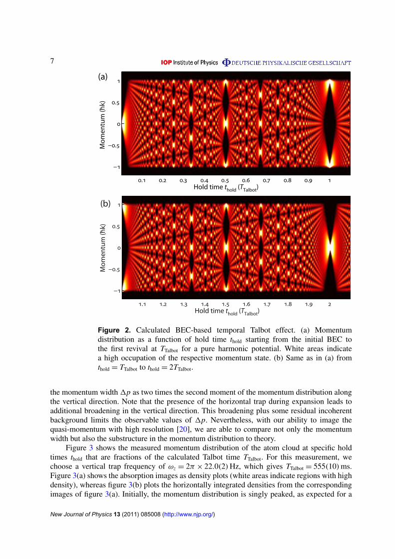
with c j(0, q) = c j(0)exp(−iq jd). Now the Talbot effect is evident. For times that are evenmultiples of TTalbot the original wave function is recovered, whereas for odd multiples theoriginal wave function appears with a shift of hk in quasi-momentum space. This realizationof the Talbot effect is nearly ideal, since no paraxial approximation is needed and since there isno limitation in time due to decreasing wave packet overlap [19]. For fractions n/m of TTalbot,m copies of the original wave function with a spacing 2hk/m appear, corresponding to thefractional Talbot effect. The evolution of the quasi-momentum distribution as a function oftime can be visualized in terms of so-called matter-wave quantum carpets [31, 32]. Such aquantum carpet, calculated by solving equation (1) numerically with parameters typical to ourexperiment, is shown in figure 2. Note that in this case the more simple calculation based onequation (3) leads to the same result. However, equation (1) gives us more flexibility in relaxingthe requirements of harmonic confinement or negligible tunnelling. We plot the distribution as aline density plot, with white areas indicating high densities. Only times that are integer multiplesof TBloch are shown. After a fast spreading of the quasi-momentum distribution, a regular patternappears at times for which one expects fractional Talbot interferences. The number of peaks inthe momentum distributions directly represents the fraction t/TTalbot. At TTalbot a refocusing tothe initial distribution occurs, shifted by hk in quasi-momentum space. The evolution is thenrepeated until at 2TTalbot the original wave function is recovered.

4. Experimental realization

For the present experiments, we choose a lattice depth of 8ER. For lattice loading, the interactionstrength is set to as = 100a0 and the external trap frequencies are changed adiabatically topopulate about 40 lattice sites. After loading, we change ωz to the final value. This changeis done sufficiently quickly (within 3 ms) to avoid a change in the initial distribution due totunnelling, but sufficiently slowly to avoid motional excitations along the z-direction. Then,within 0.1 ms, we switch off the levitating magnetic field gradient to decouple the individuallattice sites and set the scattering length to the value near as = 0a0 that gives minimaldephasing [22]. Note that the point of minimal dephasing does not correspond exactly to 0a0

as residual magnetic dipole–dipole interactions have to be taken into account [33]. The shiftis calculated to be about −0.7a0. After a variable hold time thold, which typically correspondsto hundreds of Bloch cycles with TBloch = 0.575 ms, we switch the levitation field back on in0.1 ms and ramp down the optical lattice and the dipole trap responsible for trapping in thevertical direction in 0.3 ms. The ramp is adiabatic with respect to the trap frequency of theindividual lattice sites, ensuring that the atoms stay in the lowest Bloch band and thus mappingquasi-momentum onto real momentum [34]. Before taking an absorption picture, we let thesample expand for 80 ms while it remains levitated and thus map momentum to real space. Thedipole trap responsible for horizontal trapping is not turned off immediately, but instead it isramped down slowly over the course of 50 ms to reduce spreading of the sample in the horizontaldirection. At the same time, as is kept at the value that gives minimal interactions to avoidbroadening of the sample in the vertical direction. From the absorption pictures, we calculate

New Journal of Physics 13 (2011) 085008 (http://www.njp.org/)

7

Mom

entu

m (ħ

k)

Hold time thold (TTalbot)1.1 1.2 1.3 1.4 1.5 1.6 1.7 1.8 1.9 2

−1

−0.5

0

0.5

1

Mom

entu

m (ħ

k)

Hold time thold (TTalbot)0.1 0.2 0.3 0.4 0.5 0.6 0.7 0.8 0.9 1

−1

−0.5

0

0.5

1 (a)

(b)

Figure 2. Calculated BEC-based temporal Talbot effect. (a) Momentumdistribution as a function of hold time thold starting from the initial BEC tothe first revival at TTalbot for a pure harmonic potential. White areas indicatea high occupation of the respective momentum state. (b) Same as in (a) fromthold = TTalbot to thold = 2TTalbot.

the momentum width 1p as two times the second moment of the momentum distribution alongthe vertical direction. Note that the presence of the horizontal trap during expansion leads toadditional broadening in the vertical direction. This broadening plus some residual incoherentbackground limits the observable values of 1p. Nevertheless, with our ability to image thequasi-momentum with high resolution [20], we are able to compare not only the momentumwidth but also the substructure in the momentum distribution to theory.

Figure 3 shows the measured momentum distribution of the atom cloud at specific holdtimes thold that are fractions of the calculated Talbot time TTalbot. For this measurement, wechoose a vertical trap frequency of ωz = 2π × 22.0(2) Hz, which gives TTalbot = 555(10) ms.Figure 3(a) shows the absorption images as density plots (white areas indicate regions with highdensity), whereas figure 3(b) plots the horizontally integrated densities from the correspondingimages of figure 3(a). Initially, the momentum distribution is singly peaked, as expected for a

New Journal of Physics 13 (2011) 085008 (http://www.njp.org/)

8

-1

-0.5

0

0.5

1

Mom

entu

m (ħ

k)

Hold time thold (TTalbot)

0 1/10 1/9 1/8 1/7 1/6 1/5 1/4 1/3 1/2 1

−1

−0.5

0

0.5

1

Mom

entu

m (ħ

k)

Hold time thold (TTalbot)

(a)

(b)

0 1/10 1/9 1/8 1/7 1/6 1/5 1/4 1/3 1/2 1

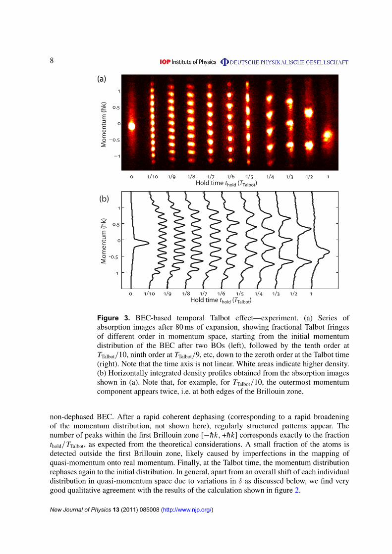
Figure 3. BEC-based temporal Talbot effect—experiment. (a) Series ofabsorption images after 80 ms of expansion, showing fractional Talbot fringesof different order in momentum space, starting from the initial momentumdistribution of the BEC after two BOs (left), followed by the tenth order atTTalbot/10, ninth order at TTalbot/9, etc, down to the zeroth order at the Talbot time(right). Note that the time axis is not linear. White areas indicate higher density.(b) Horizontally integrated density profiles obtained from the absorption imagesshown in (a). Note that, for example, for TTalbot/10, the outermost momentumcomponent appears twice, i.e. at both edges of the Brillouin zone.

non-dephased BEC. After a rapid coherent dephasing (corresponding to a rapid broadeningof the momentum distribution, not shown here), regularly structured patterns appear. Thenumber of peaks within the first Brillouin zone [−hk, +hk] corresponds exactly to the fractionthold/TTalbot, as expected from the theoretical considerations. A small fraction of the atoms isdetected outside the first Brillouin zone, likely caused by imperfections in the mapping ofquasi-momentum onto real momentum. Finally, at the Talbot time, the momentum distributionrephases again to the initial distribution. In general, apart from an overall shift of each individualdistribution in quasi-momentum space due to variations in δ as discussed below, we find verygood qualitative agreement with the results of the calculation shown in figure 2.

New Journal of Physics 13 (2011) 085008 (http://www.njp.org/)

9

0 1 2 3 4

-1

-0.5

0

0.5

1

Mom

entu

m (ħ

k)

Experimental run

0 1 2 3 4

-1

-0.5

0

0.5

1

Mom

entu

m (ħ

k)

Experimental run0 1 2 3 4

−1

−0.5

0

0.5

1

Mom

entu

m (ħ

k)

Experimental run

(a) (b)

(d)

0 1 2 3 4

−1

−0.5

0

0.5

1

Mom

entu

m (ħ

k)

Experimental run

(c)

Figure 4. Variations in the momentum distribution between successiveexperimental realizations for long hold times. (a) Absorption images of fiveindividual experimental realizations with thold = TTalbot. White areas indicatehigher density. (b) Horizontally integrated density profiles obtained from theabsorption images shown in (a). (c) Absorption images of five individualexperimental realizations with thold = TTalbot/2. (d) Horizontally integrateddensity profiles obtained from the absorption images shown in (c). Note that,in addition to the random shift in quasi-momentum space caused by δ, effects ofhorizontal dynamics, especially fragmentation and density variations along thehorizontal axis, can be observed.

Figure 4 illustrates the effect of δ on the observed patterns in quasi-momentum space.For two different hold times thold = TTalbot and thold = TTalbot/2, absorption images for severalindividual experimental realizations and the corresponding horizontally integrated densities areshown. The expected single- and double-peaked momentum patterns are reproduced from oneexperimental realization to the next, but they experience a varying shift in quasi-momentumspace. As a consequence of the periodic structure of quasi-momentum space, a peak that islocated near one edge of the Brillouin zone also reappears at the opposite edge. The maximumpossible shift of the pattern in quasi-momentum space due to δ increases with hold time and

New Journal of Physics 13 (2011) 085008 (http://www.njp.org/)

10

is calculated to be ±hk × thold/TTalbot. This is why the patterns shown in figure 3, for example,at thold = TTalbot or at thold = TTalbot/2, agree with the calculated patterns only modulo the shiftin quasi-momentum space. Note that, alternatively, we could have chosen to present in figure 3selected patterns from a sufficiently large sample of measurements, for example, the one fromexperimental run 4 for thold = TTalbot or the one from experimental run 1 for thold = TTalbot/2shown in figure 4.

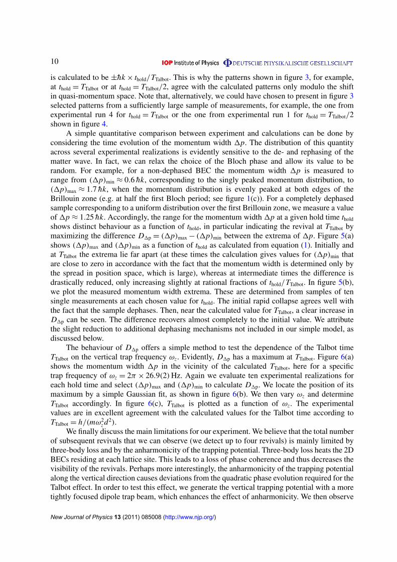
A simple quantitative comparison between experiment and calculations can be done byconsidering the time evolution of the momentum width 1p. The distribution of this quantityacross several experimental realizations is evidently sensitive to the de- and rephasing of thematter wave. In fact, we can relax the choice of the Bloch phase and allow its value to berandom. For example, for a non-dephased BEC the momentum width 1p is measured torange from (1p)min ≈ 0.6 hk, corresponding to the singly peaked momentum distribution, to(1p)max ≈ 1.7 hk, when the momentum distribution is evenly peaked at both edges of theBrillouin zone (e.g. at half the first Bloch period; see figure 1(c)). For a completely dephasedsample corresponding to a uniform distribution over the first Brillouin zone, we measure a valueof 1p ≈ 1.25 hk. Accordingly, the range for the momentum width 1p at a given hold time thold

shows distinct behaviour as a function of thold, in particular indicating the revival at TTalbot bymaximizing the difference D1p = (1p)max − (1p)min between the extrema of 1p. Figure 5(a)shows (1p)max and (1p)min as a function of thold as calculated from equation (1). Initially andat TTalbot the extrema lie far apart (at these times the calculation gives values for (1p)min thatare close to zero in accordance with the fact that the momentum width is determined only bythe spread in position space, which is large), whereas at intermediate times the difference isdrastically reduced, only increasing slightly at rational fractions of thold/TTalbot. In figure 5(b),we plot the measured momentum width extrema. These are determined from samples of tensingle measurements at each chosen value for thold. The initial rapid collapse agrees well withthe fact that the sample dephases. Then, near the calculated value for TTalbot, a clear increase inD1p can be seen. The difference recovers almost completely to the initial value. We attributethe slight reduction to additional dephasing mechanisms not included in our simple model, asdiscussed below.

The behaviour of D1p offers a simple method to test the dependence of the Talbot timeTTalbot on the vertical trap frequency ωz. Evidently, D1p has a maximum at TTalbot. Figure 6(a)shows the momentum width 1p in the vicinity of the calculated TTalbot, here for a specifictrap frequency of ωz = 2π × 26.9(2) Hz. Again we evaluate ten experimental realizations foreach hold time and select (1p)max and (1p)min to calculate D1p. We locate the position of itsmaximum by a simple Gaussian fit, as shown in figure 6(b). We then vary ωz and determineTTalbot accordingly. In figure 6(c), TTalbot is plotted as a function of ωz. The experimentalvalues are in excellent agreement with the calculated values for the Talbot time according toTTalbot = h/(mω2

z d2).We finally discuss the main limitations for our experiment. We believe that the total number

of subsequent revivals that we can observe (we detect up to four revivals) is mainly limited bythree-body loss and by the anharmonicity of the trapping potential. Three-body loss heats the 2DBECs residing at each lattice site. This leads to a loss of phase coherence and thus decreases thevisibility of the revivals. Perhaps more interestingly, the anharmonicity of the trapping potentialalong the vertical direction causes deviations from the quadratic phase evolution required for theTalbot effect. In order to test this effect, we generate the vertical trapping potential with a moretightly focused dipole trap beam, which enhances the effect of anharmonicity. We then observe

New Journal of Physics 13 (2011) 085008 (http://www.njp.org/)

11

0.1 0.2 0.3 0.4 0.5 0.6 0.7 0.8 0.9 10

0.5

1

1.5

2

Mom

entu

m w

idth

∆p

(ħk)

Hold time tHold (TTalbot)

0.1 0.2 0.3 0.4 0.5 0.6 0.7 0.8 0.9 10.5

1

1.5

2

Mom

entu

m w

idth

Δp

(ħk)

Hold time thold (TTalbot)

(a)

(b)

Figure 5. Talbot revival as evidenced by the spread of momentum width 1p.(a) Calculated (1p)max (blue diamonds) and (1p)min (black circles) as a functionof thold in units of TTalbot. (b) Measurement of (1p)max (blue diamonds) and(1p)min (black circles) as a function of thold in units of TTalbot for a vertical trapfrequency of ωz = 2π × 22.0(2) Hz. The extrema are determined from a sampleof ten single experimental realizations for each value of thold.

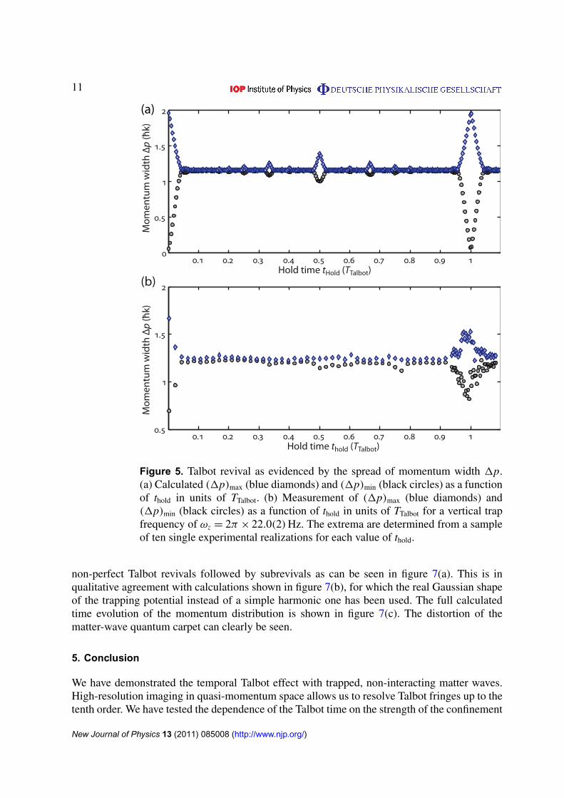
non-perfect Talbot revivals followed by subrevivals as can be seen in figure 7(a). This is inqualitative agreement with calculations shown in figure 7(b), for which the real Gaussian shapeof the trapping potential instead of a simple harmonic one has been used. The full calculatedtime evolution of the momentum distribution is shown in figure 7(c). The distortion of thematter-wave quantum carpet can clearly be seen.

5. Conclusion

We have demonstrated the temporal Talbot effect with trapped, non-interacting matter waves.High-resolution imaging in quasi-momentum space allows us to resolve Talbot fringes up to thetenth order. We have tested the dependence of the Talbot time on the strength of the confinement

New Journal of Physics 13 (2011) 085008 (http://www.njp.org/)

12

20 25 30 35 40 45 50100

200

300

400

500

600

Talb

ot ti

me T T

albo

t (m

s)

Trap frequency νz (Hz)

340 360 380

0.9

1

1.1

1.2

1.3

1.4

1.5

1.6

p (ħ

k)

Hold time thold (ms)340 360 380

0

0.1

0.2

0.3

0.4

0.5

0.6

∆p (ħ

k)

Hold time thold (ms)

(a) (b)

(c)

Figure 6. Talbot time TTalbot as a function of external confinement strength.(a) Momentum width 1p in the vicinity of the expected TTalbot for a dipoletrap frequency of ωz = 2π × 26.9(2) Hz for ten single experimental realizations(black circles). The extrema (1p)max and (1p)min are indicated as red diamonds.(b) Calculated D1p for the measured extrema in (a). The solid line representsa Gaussian fit, from which TTalbot is derived. (c) Dependence of TTalbot ontrap frequency νz = ωz/(2π). The black (blue) circles (diamonds) representmeasurements for which the external harmonic trap is generated by the dipoletrap beam with a 46 µm (144 µm) beam waist. The solid line gives the calculatedvalues for TTalbot. The vertical error bars are the 1σ uncertainty of the maximumposition of the Gaussian fit as shown in (b). The horizontal error bars are equalto or smaller than symbol size.

and have found very good agreement with the calculated value. We find that the interferencepattern is sensitive to the anharmonicity of the trapping potential. In principle, the detailedstructure of the interference pattern and the precise revival times are sensitive probes for forcegradients and interactions between atoms. The weak magnetic dipole–dipole interaction, for

New Journal of Physics 13 (2011) 085008 (http://www.njp.org/)

13

240 260 280 300

0.5

1

1.5

Mom

entu

m w

idth

∆p

(ħk)

Hold time tHold (ms)

Mom

entu

m (ħ

k)

Hold time thold (TTalbot)0.1 0.2 0.3 0.4 0.5 0.6 0.7 0.8 0.9 1

−1

−0.5

0

0.5

1

240 260 280 300

0.9

1

1.1

1.2

1.3

1.4

1.5

1.6

Mom

entu

m w

idth

Δp

(ħk)

Hold time thold (ms)

(a) (b)

(c)

Figure 7. The effect of anharmonic trapping potential on momentum distribution.(a) Momentum width 1p in the vicinity of the expected TTalbot for a dipole trapfrequency of 2π × 31.1(2) Hz for ten single experimental realizations (blackcircles). The vertical dipole trap is created by the more tightly focused dipoletrap beam with a beam waist of 46 µm. The extrema (1p)max and (1p)min areindicated as red diamonds. (b) Calculated (1p)max and (1p)min in the vicinityof the expected TTalbot for the same experimental parameters as in (a). For thetrapping potential, the real Gaussian shape of the dipole trap is used. (c) Fullcalculation of the momentum distribution as a function of hold time thold usingthe same parameters as in (b).

example, has recently been investigated in the context of matter-wave interferometry [33].Matter-wave interferometry in the Talbot regime could potentially be used to examine in detailthe effect of the long-range nature of such an interaction. Similarly, a spatially dependent forcelike the Casimir–Polder force [35–37] near a surface could be investigated through its influenceon the Talbot interference pattern.

New Journal of Physics 13 (2011) 085008 (http://www.njp.org/)

14

Acknowledgments

We are indebted to R Grimm for generous support and we thank A Daley for valuablediscussions. We gratefully acknowledge funding by the Austrian Science Fund (FWF) withinproject I153-N16 and within the framework of the European Science Foundation (ESF)EuroQUASAR collective research project QuDeGPM.

References

[1] Cronin A D, Schmiedmayer J and Pritchard D E 2009 Rev. Mod. Phys. 81 1051–129[2] Davisson C and Germer L H 1927 Phys. Rev. 30 705–40[3] Jönsson C 1961 Z. Phys. 161 454–74[4] Rauch H, Treimer W and Bonse U 1974 Phys. Lett. A 47 369–71[5] Reisinger T, Patel A A, Reingruber H, Fladischer K, Ernst W E, Bracco G, Smith H I and Holst B 2009 Phys.

Rev. A 79 053823[6] Anderson M H, Ensher J R, Matthews M R, Wieman C E and Cornell E A 1995 Science 269 198[7] Davis K B, Mewes M O, Andrews M R, van Druten N J, Durfee D S, Kurn D M and Ketterle W 1995 Phys.

Rev. Lett. 75 3969–73[8] Berry M, Marzoli I and Schleich W P 2001 Phys. World 14 39–44[9] Talbot H F 1836 Phil. Magn. 9 401

[10] Rayleigh L 1881 Phil. Magn. 11 196–205[11] Patorski K 1989 Prog. Opt. 27 1–108[12] Schmiedmayer J, Ekstrom C R, Chapman M S, Hammond T D and Pritchard D E 1993 Fundamentals

of Quantum Optics III Proc. Kühtai Austria ed F Ehlotzky (Lecture Notes in Physics vol 420) (Berlin:Springer)

[13] Chapman M S, Ekstrom C R, Hammond T D, Schmiedmayer J, Tannian B E, Wehinger S and Pritchard D E1995 Phys. Rev. A 51 R14–7

[14] Nowak S, Kurtsiefer Ch, Pfau T and David C 1997 Opt. Lett. 22 1430–2[15] Lau E 1948 Ann. Phys. 6 417[16] Clauser J F and Li S 1994 Phys. Rev. A 49 R2213–6[17] Brezger B, Hackermüller L, Uttenthaler S, Petschinka J, Arndt M and Zeilinger A 2002 Phys. Rev. Lett.

88 100404[18] Gerlich S et al 2007 Nature Phys. 3 711–5[19] Deng L, Hagley E W, Denschlag J, Simsarian J E, Edwards M, Clark C W, Helmerson K, Rolston S L and

Phillips W D 1999 Phys. Rev. Lett. 83 5407–11[20] Gustavsson M, Haller E, Mark M J, Danzl J G, Hart R, Daley A J and Nägerl H-C 2010 New J. Phys.

12 065029[21] Li W, Tuchman A K, Chien H-C and Kasevich M A 2007 Phys. Rev. Lett. 98 040402[22] Gustavsson M, Haller E, Mark M J, Danzl J G, Rojas-Kopeinig G and Nägerl H-C 2008 Phys. Rev. Lett.

100 080404[23] Weber T, Herbig J, Mark M, Nägerl H-C and Grimm R 2003 Science 299 232[24] Kraemer T, Herbig J, Mark M, Weber T, Chin C, Nägerl H C and Grimm R 2004 Appl. Phys. B 79 1013–9[25] Chin C, Vuletic V, Kerman A J, Chu S, Tiesinga E, Leo P J and Williams C J 2004 Phys. Rev. A 70 032701[26] Liem A, Limpert J, Zellmer H and Tünnermann A 2003 Opt. Lett. 28 1537–9[27] Smerzi A and Trombettoni A 2003 Phys. Rev. A 68 023613[28] Witthaut D, Werder M, Mossmann S and Korsch H J 2005 Phys. Rev. E 71 036625[29] Ben Dahan M, Peik E, Reichel J, Castin Y and Salomon C 1996 Phys. Rev. Lett. 76 4508–11[30] Anderson B P and Kasevich M A 1998 Science 282 1686[31] Kaplan A E, Marzoli I, Lamb W E Jr and Schleich W P 2000 Phys. Rev. A 61 032101

New Journal of Physics 13 (2011) 085008 (http://www.njp.org/)

15

[32] Ruostekoski J, Kneer B, Schleich W P and Rempe G 2001 Phys. Rev. A 63 043613[33] Fattori M, Roati G, Deissler B, D’Errico C, Zaccanti M, Jona-Lasinio M, Santos L, Inguscio M and Modugno

G 2008 Phys. Rev. Lett. 101 190405[34] Kastberg A, Phillips W D, Rolston S L, Spreeuw R J C and Jessen P S 2008 Phys. Rev. Lett. 74 1542–5[35] Casimir H B G and Polder D 1948 Phys. Rev. 73 360[36] Harber D M, Obrecht J M, McGuirk J M and Cornell E A 2005 Phys. Rev. A 72 033610[37] Chwedenczuk J, Pezzé L, Piazza F and Smerzi A 2010 Phys. Rev. A 82 032104

New Journal of Physics 13 (2011) 085008 (http://www.njp.org/)