ARTICLE

Demographic histories and genetic diversity acrosspinnipeds are shaped by human exploitation,ecology and life-historyM.A. Stoffel1,2, E. Humble1,3, A.J. Paijmans 1, K. Acevedo-Whitehouse4, B.L. Chilvers5, B. Dickerson6,

F. Galimberti 7, N.J. Gemmell 8, S.D. Goldsworthy9, H.J. Nichols2,18,19, O. Krüger1, S. Negro10,20,

A. Osborne11, T. Pastor12, B.C. Robertson13, S. Sanvito 7, J.K. Schultz14, A.B.A. Shafer15, J.B.W. Wolf16,17 &

J.I. Hoffman1,3

A central paradigm in conservation biology is that population bottlenecks reduce genetic

diversity and population viability. In an era of biodiversity loss and climate change, under-

standing the determinants and consequences of bottlenecks is therefore an important

challenge. However, as most studies focus on single species, the multitude of potential

drivers and the consequences of bottlenecks remain elusive. Here, we combined genetic data

from over 11,000 individuals of 30 pinniped species with demographic, ecological and life

history data to evaluate the consequences of commercial exploitation by 18th and 19th

century sealers. We show that around one third of these species exhibit strong signatures of

recent population declines. Bottleneck strength is associated with breeding habitat and

mating system variation, and together with global abundance explains much of the variation

in genetic diversity across species. Overall, bottleneck intensity is unrelated to IUCN status,

although the three most heavily bottlenecked species are endangered. Our study reveals an

unforeseen interplay between human exploitation, animal biology, demographic declines and

genetic diversity.

DOI: 10.1038/s41467-018-06695-z OPEN

1 Department of Animal Behaviour, Bielefeld University, Postfach 100131, 33501 Bielefeld, Germany. 2 School of Natural Sciences and Psychology, Faculty ofScience, Liverpool John Moores University, Liverpool L3 3AF, UK. 3 British Antarctic Survey, High Cross, Madingley Road, Cambridge CB3 OET, UK. 4 Unit forBasic and Applied Microbiology, School of Natural Sciences, Autonomous University of Queretaro, Avenida de las Ciencias S/N, Queretaro 76230, Mexico.5Wildbase, Institute of Veterinary, Animal and Biomedical Science, Massey University, Private Bag 11222, Palmerston North 4442, New Zealand. 6NationalMarine Mammal Laboratory, Alaska Fisheries Science Center, National Marine Fisheries Service, National Oceanic and Atmospheric Administration, Seattle98115 WA, USA. 7 Elephant Seal Research Group, Sea Lion Island, FIQQ 1ZZ, Falkland Islands. 8Department of Anatomy, University of Otago, PO Box 56,Dunedin 9054, New Zealand. 9 South Australian Research and Development Institute, West Beach, SA 5024, Australia. 10 UMR de Génétique Quantitative etÉvolution – Le Moulon, INRA, Université Paris-Sud, CNRS, AgroParisTech, Université Paris-Saclay, Gif-sur-Yvette 91190, France. 11 School of BiologicalSciences, University of Canterbury, Private Bag 4800, Christchurch, New Zealand 8140. 12 EUROPARC Federation, Carretera de l’Església, 92, 08017Barcelona, Spain. 13 Department of Zoology, University of Otago, PO Box 56, Dunedin 9054, New Zealand. 14 National Marine Fisheries Service, NationalOceanic and Atmospheric Administration, 1315 East West Highway, Silver Spring, MD 20910, USA. 15 Forensic Science & Environmental Life Sciences, TrentUniversity, Peterborough, ON, Canada K9J 7B8. 16 Division of Evolutionary Biology, Faculty of Biology, LMU Munich, Planegg-Martinstried, Munich 82152,Germany. 17 Science of Life Laboratory and Department of Evolutionary Biology, Uppsala University, Uppsala 752 36, Sweden. 18Present address: Departmentof Animal Behaviour Bielefeld University, Postfach 100131 33501 Bielefeld, Germany. 19Present address: Department of Biosciences, Swansea University,Swansea SA2 8PP, UK. 20Present address: GIGA-R, Medical Genomics - BIO3, Université of Liège, Liège 4000, Belgium. Correspondence and requests formaterials should be addressed to J.I.H. (email: joseph.hoffman@uni-bielefeld.de)

NATURE COMMUNICATIONS | (2018) 9:4836 | DOI: 10.1038/s41467-018-06695-z | www.nature.com/naturecommunications 1

1234

5678

90():,;

Unravelling the demographic histories of species is a fun-damental goal of population biology and has tremendousimplications for understanding the genetic variability

observed today1,2. Of particular interest are sharp reductions inthe effective population size (Ne) known as populationbottlenecks3,4, which may negatively impact the viability andadaptive evolutionary potential of species through a variety ofstochastic demographic processes and the loss of genetic diver-sity5–8. Specifically, small bottlenecked populations have elevatedlevels of inbreeding and genetic drift, which decrease geneticvariability and can lead to the fixation of mildly deleterious allelesand ultimately drive a vortex of extinction6,8–10. Hence, investi-gating the bottleneck histories of wild populations and theirdeterminants and consequences is more critical than ever before,as we live in an era where global anthropogenic alteration anddestruction of natural habitats are driving species declines on anunprecedented scale11,12.

Unfortunately, detailed information about past populationdeclines across species is sparse because historical population sizeestimates are often either non-existent or highly uncertain13,14. Aversatile solution for inferring population bottlenecks from asingle sample of individuals is to compare levels of observed andexpected genetic diversity, the latter of which can be simulatedunder virtually any demographic scenario based on the coales-cent15–17. A variety of approaches based on this principle havebeen developed, one of the most widely used being theheterozygosity-excess test, which compares the heterozygosity ofa panel of neutral genetic markers to the expectation in a stablepopulation under mutation-drift equilibrium18. Although theo-retically well grounded, these methods are highly sensitive to theassumed mutation model, which is seldom known19. A moresophisticated framework for inferring demographic histories iscoalescent-based approximate Bayesian computation (ABC)20.ABC has the compelling advantages of making it possible to (i)compare virtually any demographic scenario as long as it can besimulated, (ii) estimate key parameters of the model such as thebottleneck effective population size and (iii) incorporate uncer-tainty in the specification of models by defining priors. Due tothis flexibility, ABC has become a state of the art approach forinferring population bottlenecks as well as demographic historiesin general20–29.

Although the widespread availability of neutral molecularmarkers such as microsatellites has facilitated numerous geneticstudies of bottlenecks in wild populations, the vast majority ofstudies focused exclusively on single species and were confined totesting for the presence or absence of bottlenecks. We thereforeknow very little about the intensity of demographic declines andhow these are influenced by anthropogenic impacts as well as byfactors intrinsic to a given species. For example, species occupy-ing breeding habitats that are more accessible to humans wouldbe expected to be at higher risk of declines, while species withhighly skewed mating systems tend to have lower effectivepopulation sizes30 and might also experience stronger demo-graphic declines as only a fraction of individuals contributetowards the genetic makeup of subsequent generations. Conse-quently, to disentangle the forces shaping population bottlenecks,we need comparative studies incorporating genetic, ecological andlife-history data from multiple closely related species within aconsistent analytical framework.

Another question that remains elusive due to a lack of com-parative studies is to what extent recent bottlenecks haveimpacted the genetic diversity of wild populations. While anumber of influential studies of heavily bottlenecked species haveindeed found very low levels of genetic variability31–34, othershave reported unexpectedly high genetic variation after suppo-sedly strong population declines23,35–38. Hence, it is not yet clear

how population size changes contribute towards one of the mostfundamental questions in evolutionary genetics—how and whygenetic diversity varies across species2,39–41. To tackle this ques-tion, we need to compare closely related species because deeplydivergent taxa vary so profoundly in their genetic diversity due todifferences in their life-history strategies that any effects causedby variation in Ne will be hard to detect and decipher40,41.

Finally, the relative contributions of genetic diversity anddemographic factors towards extinction risk remain unclear.While historically there has been a debate about the immediateimportance of genetic factors towards species viability5,7, there isnow growing evidence that low genetic diversity increasesextinction risk8,42 and on a broader scale that threatened speciestend to show reduced diversity7. Nevertheless, due to a lack ofstudies measuring bottlenecks consistently across species, itremains an open question as to how the loss of genetic diversitycaused by demographic declines ultimately translates into a spe-cies' extinction risk, which can be assessed by its InternationalUnion for Conservation of Nature (IUCN) status.

An outstanding opportunity to address these questions isprovided by the pinnipeds, a clade of marine carnivores inha-biting nearly all marine environments ranging from the poles tothe tropics and showing remarkable variation in their ecologicaland life-history adaptations43. Pinnipeds include some of themost extreme examples of commercial exploitation known toman, with several species including the northern elephant sealhaving been driven to the brink of extinction for their fur andblubber by 18th to early 20th century sealers13. By contrast, otherpinniped species inhabiting pristine environments such as Ant-arctica have probably had very little contact with humans13.Hence, pinnipeds show large differences in their demographichistories within the highly constrained time window of com-mercial sealing and thereby represent a unique natural experi-ment for exploring the causes and consequences of recentbottlenecks.

Here, we conducted a broad-scale comparative analysis ofpopulation bottlenecks using a combination of genetic, ecologicaland life-history data for 30 pinniped species. We inferred thestrength of historical declines across species from the genetic datausing two complimentary coalescent-based approaches,heterozygosity-excess and ABC. Heterozygosity-excess was usedas a measure of the relative strength of recent population declines,while a consistent ABC framework was used to evaluate theprobability of each species having experienced a severe bottleneckduring the known timeframe of commercial exploitation, as wellas to estimate relevant model parameters. Finally, we usedBayesian phylogenetic mixed models to investigate the potentialcauses and consequences of past bottlenecks while controlling forphylogenetic relatedness among species. We hypothesised that (i)extreme variation in the extent to which species were exploited byman should be reflected in their genetic bottleneck signatures; (ii)ecological and life-history traits could have an impact on thestrength of bottleneck signatures across species; (iii) past bottle-necks should reduce contemporary genetic diversity; and (iv)heavily bottlenecked species with reduced genetic diversity will bemore likely to be of conservation concern.

We report striking variation in genetic bottleneck signaturesacross pinnipeds, with 11 species exhibiting strong genetic sig-natures of population declines and estimated bottleneck effectivepopulation sizes reflecting just a few tens of surviving individualsin the most extreme cases. Despite being caused by humanexploitation, these genetic bottlenecks are mediated by bothbreeding habitat and mating system variation, implying thatspecies ecology and life-history contribute towards responses toanthropogenic exploitation. Furthermore, up to five-fold varia-tion in genetic diversity across species is explained by a

ARTICLE NATURE COMMUNICATIONS | DOI: 10.1038/s41467-018-06695-z

2 NATURE COMMUNICATIONS | (2018) 9:4836 | DOI: 10.1038/s41467-018-06695-z | www.nature.com/naturecommunications

combination of bottleneck history, global abundance and breed-ing habitat. Finally, exploring the consequences of historicalbottlenecks for conservation, we show that genetic bottlenecksignatures are unrelated to IUCN status across all species,although three of the four most heavily bottlenecked species arecurrently endangered. We conclude that the genetic consequencesof anthropogenic exploitation depend heavily on a species’ biol-ogy, while quantifying demographic histories can substantiallycontribute to understanding patterns of genetic diversity acrossspecies.

ResultsGenetic data. We analysed a combination of published and newlygenerated microsatellite data from 30 pinniped species, with amedian of 253 individuals and 14 loci per species (see Methodsand Supplementary Table 1 for details). Measures of geneticdiversity, standardised across datasets as the average per tenindividuals, varied considerably across the pinniped phylogeny,with observed heterozygosity (Ho) and allelic richness (Ar)varying by over two and almost five-fold respectively acrossspecies (Supplementary Table 2). Both of these measures werehighly correlated (r= 0.92) and tended to be higher in icebreeding seals, intermediate in fur seals and sea lions, and sub-stantially lower in a handful of species including northern ele-phant seals and monk seals (Fig. 1a).

Bottleneck inference. We used two different coalescent-basedapproaches to infer the extent of recent population bottlenecks.First, the amount of heterozygosity-excess at selectively neutralloci such as microsatellites is an indicator of recent bottlenecksbecause during a population decline the number of alleles

decreases faster than heterozygosity3. Recent bottlenecks there-fore generate a transient excess of heterozygosity relative to apopulation at equilibrium with an equivalent number of alleles18.Here, we quantified the proportion of loci in heterozygosity-excess (prophet-exc) for each species, which was highly repeatableacross a range of mutation models (see Methods and Supple-mentary Table 3). Consequently, we focused on a two-phasemodel with 80% single-step mutations (TPM80), which is broadlyin line with mammalian mutation model estimates from the lit-erature44 as well as posterior estimates from our ABC analysis(Supplementary Table 4B, Supplementary Fig. 5). Figure 1bshows a heatmap of prophet-exc across species, which is boundedbetween zero (all loci show heterozygosity-deficiency, an indi-cator of recent expansion) and one (all loci show heterozygosity-excess, an indicator of recent decline) whereby 0.5 is the expec-tation for a stable population. Considerable heterogeneity wasfound across species, with northern and southern elephant seals,grey seals, Guadalupe fur seals and Antarctic fur seals showingthe strongest bottlenecks signals. By contrast, the majority of ice-breeding seals exhibited heterozygosity-deficiency, consistentwith historical population expansions.

Second, we used ABC to select between a bottleneck and a non-bottleneck model as well as to estimate posterior distributions ofrelevant parameters. To optimally capture recent population sizechanges across species, we allowed Ne to vary from pre-bottleneckto post-bottleneck in both models within realistic priors (seeMethods for details) while the bottleneck model also included asevere decrease in Ne to below 500 during the time of peaksealing. Therefore, both models incorporate longer-term declinesor expansions within realistic bounds for all species but only thebottleneck model captures a recent and severe decrease in Ne due

Global abundance

IUCN rating

Breeding habitat

Ice Land

EndangeredVulnerableNear threatenedLeast concern Weddell seal (WS)

Leopard seal (LS)Crabeater seal (CS)Ross seal (RoS)Southern elephant seal (SES)Northern elephant seal (NES)

Ringed seal (RS)Baltic ringed seal (BRS)Saimaa ringed seal (SRS)Ladoga ringed seal (LRS)Mediterranean monk seal (MMS)Hawaiian monk seal (HMS)

Grey seal (GS)Harbor seal (HS)Hooded seal (HoodS)Bearded seal (BS)Galapagos fur seal (GFS)

South American sea lion (SASL)

South American fur seal (SAFS)

New Zealand sea lion (NZSL)

New Zealand fur seal (NZFS)

Antarctic fur seal (AntFS)Subantarctic fur seal (SAntFS)

Guadalupe fur seal (GuaFS)

Standardizedgenetic diversity

–2 –1 10 0 012 0.5 50 100

Prop. of loci withheterozyg. –excess

ABC modelprobability %

Walrus (W)Ar Ho prophet–exc pnon–botpbot

Northern fur seal (NFS)Steller sea lion (SSL)California sea lion (CSL)Galapagos sea lion (GSL)Australian fur seal (AFS)

103 104 105 106

a b c

Fig. 1 Patterns of genetic diversity and bottleneck signatures across the pinnipeds. The phylogeny shows 30 species with branches colour coded accordingto breeding habitat and tip points coloured and sized according to their IUCN status and global abundance respectively. a Shows two genetic diversitymeasures, allelic richness (Ar) and observed heterozygosity (Ho), which have been standardised by randomly sub-sampling ten individuals from eachdataset 1000 times with replacement and calculating the corresponding mean. b Shows the proportion of loci in heterozygosity-excess (prophet-exc)calculated for the TPM80 model (see Methods for details). c Summarises the ABC model selection results, with posterior probabilities corresponding tothe bottleneck versus non-bottleneck model. The raw data are provided in Supplementary Tables 2 and 3

NATURE COMMUNICATIONS | DOI: 10.1038/s41467-018-06695-z ARTICLE

NATURE COMMUNICATIONS | (2018) 9:4836 | DOI: 10.1038/s41467-018-06695-z | www.nature.com/naturecommunications 3

to anthropogenic exploitation. ABC was clearly able to distin-guish between the two models, with simulations under thebottleneck model being correctly classified 85% of the time andsimulations under the non-bottleneck model being correctlyclassified 89% of the time (Supplementary Fig. 1). A smallamount of overlap between the models and therefore misclassi-fication is unavoidable because both models were specified usingbroad priors to optimally fit a variety of species with vastlydifferent population sizes. For each species, however, thepreferred model showed a good fit to the observed data (all p-values > 0.05, Supplementary Table 5)45. As another indicator ofmodel quality, posterior predictive checks21,46 showed that thepreferred models across all species were largely able to reproducethe relevant observed summary statistics (Supplementary Fig. 2).The posterior bottleneck model probability (pbot) varied sub-stantially across species and was strongly but imperfectlycorrelated with prophet-exc (posterior median and 95% credibleintervals; β= 0.17 [0.04, 0.28], R2marginal= 0.32 [0.03, 0.59], seeSupplementary Fig. 3). For 11 species, the bottleneck model wassupported with a higher probability than the non-bottleneckmodel (i.e., pbot > 0.5, see Supplementary Table 3). Subsequentparameter estimation was therefore based on the bottleneckmodel for eleven species and on the non-bottleneck model for theother 19 species.

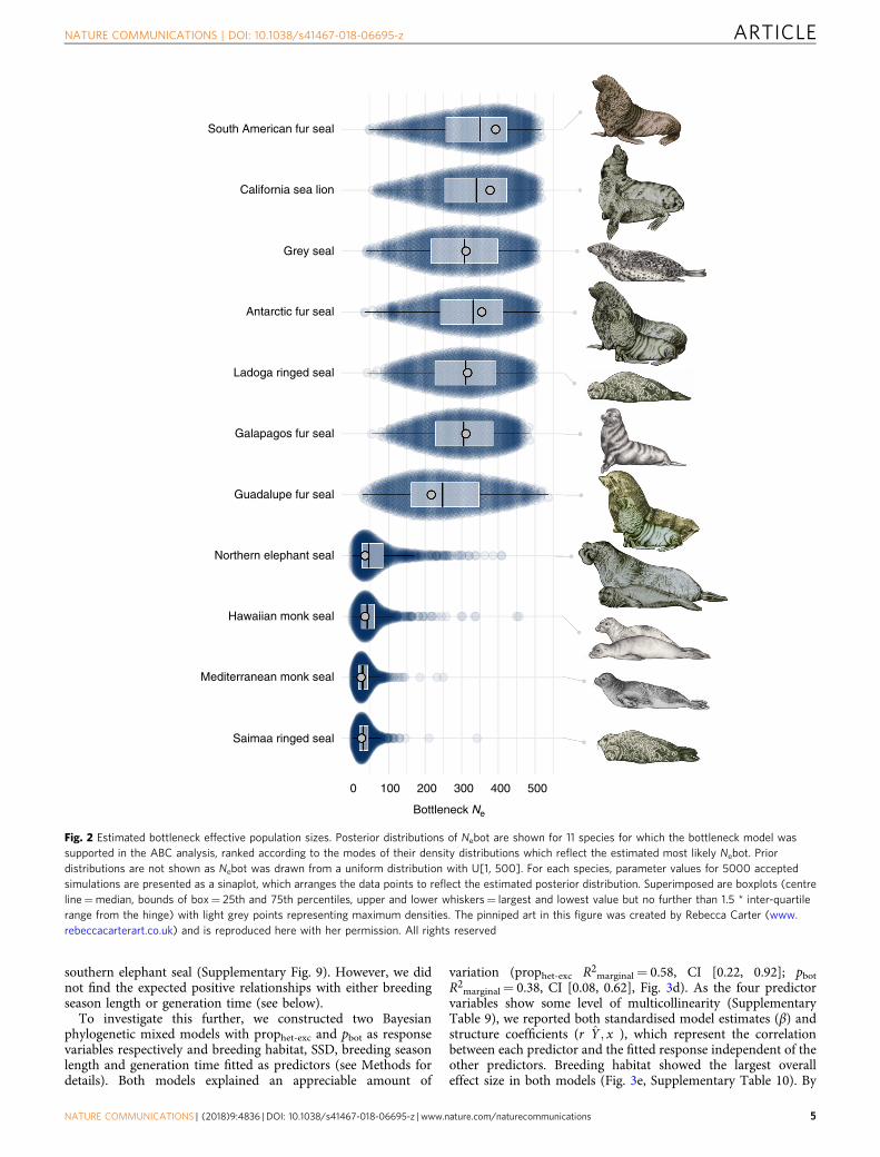
Under the bottleneck model, prediction errors from the cross-validation were well below one for the bottleneck effectivepopulation size (Nebot, Supplementary Table 4A and Supple-mentary Fig. 4) and mutation rate (µ, Supplementary Table 4A)indicating that posterior estimates contain information about theunderlying true parameter values. Similarly, under the non-bottleneck model, µ (Supplementary Table 4B) and the parameterdescribing the proportion of multi-step mutations (GSMpar,Supplementary Table 4B) were informative. By contrast, althoughthe pre-bottleneck effective population size (Nehist) also had aprediction error below one in both models, visual inspection ofthe cross-validation results revealed high variation in theestimates and a systematic underestimation of larger Nehistvalues, so this parameter was not considered further. Figure 2shows the eleven bottlenecked species ranked in descendingorder of estimated posterior modal Nebot (see also SupplementaryTable 4A). The parameter estimates were indicative of strong bot-tlenecks (i.e., 200 <Nebot < 500) in seven species includingboth phocids and otariids, while even smaller Nebot values (i.e.,Nebot < 50) were estimated for four phocids comprisingthe landlocked Saimaa ringed seal, both monk seal species andthe northern elephant seal. Mutation rate estimates wereremarkably consistent across species, with modes of the posteriordistributions typically varying around 1 × 10−4 (SupplementaryFig. 5 and Supplementary Table 4), while GSMpar acrossspecies typically varied between around 0.2 and 0.3 (SeeSupplementary Fig. 6 and Supplementary Table 4B). Therefore,although studies of individual species are usually limited byuncertainty over the underlying mutation characteristics, ourABC analyses converged on similar estimates of mutation modeland rate across species, allowing us to appropriately parameteriseour bottleneck analyses.

To explore whether our results could be affected by populationstructure, we used STRUCTURE47 to infer the most likelynumber of genetic clusters (K) across all datasets (see Supple-mentary Table 6). For all of the species for which the bestsupported value of K was more than one (n= 12), we recalculatedgenetic summary statistics and repeated the bottleneck analysesbased on individuals comprising the largest cluster. Using thelargest genetic clusters did not appreciably affect our results, withrepeatabilities for the genetic summary statistics and bottlenecksignatures all being greater than 0.9 (see Supplementary Table

7 for repeatabilities and Supplementary Fig. 7, which is virtuallyidentical to Fig. 1).

Furthermore, we tested all loci from each dataset for deviationsfrom Hardy-Weinberg equilibrium (HWE, see the Methods fordetails). Overall, 6% of loci were found to deviate from HWE inboth χ2 and exact tests after table-wide Bonferroni correction formultiple testing. To investigate whether including these loci couldhave affected our results, we recalculated the genetic summarystatistics and repeated our bottleneck analyses after excludingthem. The results remained largely unaltered, with repeatabilitiesall being greater than 0.97 (see Supplementary Table 8 andSupplementary Fig. 8).

Finally, we considered the possibility that our inference ofrecent bottlenecks could have been confounded by events furtherback in a species’ history. In particular, increased ice cover duringthe last glacial maximum (LGM) could have reduced habitatavailability and consequently population sizes48–52. We thereforetested whether small population sizes during the LGM followedby expansions could result in similar genetic patterns acrosspinnipeds to recent bottlenecks caused by anthropogenicexploitation (for details, see Supplementary Note 2). Specifically,we used ABC to simulate two additional demographic scenariosthat were identical to the bottleneck and non-bottleneck modelsbut which also incorporated a small population size during theLGM and subsequent expansion. ABC was not able to reliablydistinguish between the two bottleneck models: correct classifica-tion rates were substantially lower at 64% for the bottleneckmodel and 60% for the bottleneck model incorporating post-glacial expansion. Similarly, the two non-bottleneck models hadrelatively poor classification rates (60% for the non-bottleneckmodel and 66% for the non-bottleneck model incorporatingexpansion). These rates are much lower than in our main analysisbased on two models, indicating that ABC cannot reliablydistinguish on the basis of our data between broadly equivalentmodels that do and do not include ice age effects. Regardless, all11 of the species that supported the bottleneck model in the mainanalysis again showed the highest probability for one of the twomodels that incorporated a recent bottleneck (SupplementaryTable 11). The fact that none of these species supported the non-bottleneck model with postglacial expansion indicates that thereduction in genetic diversity produced by a recent bottleneck canbe clearly distinguished from the reduction in diversity due to asmall population size at the end of the last ice age. This is to beexpected as many of our summary statistics such as the M-ratioare sensitive towards recent population size changes53.

Factors affecting bottleneck history. Conceivably both ecologicaland life-history variables could have impacted the extent to whichcommercial exploitation affected different pinniped species. Wetherefore investigated the effects of four different variables onbottleneck signatures. First, we hypothesised that breeding habitatwould be important as ice-breeding species are less accessible andmore widely dispersed than their land-breeding counterparts.Second, we considered sexual size dimorphism (SSD) an impor-tant life-history variable as species with a high SSD aggregate indenser breeding colonies, making them more valuable to hunters,and polygyny reduces effective population size. Third, the lengthof the breeding season may have impacted the vulnerability of agiven species to exploitation and finally, generation time couldpotentially mediate population recovery. We found clear differ-ences between ice-breeding and land-breeding seals in bothprophet-exc and pbot, with land-breeders on average showingstronger bottleneck signatures (Fig. 3a, b). In addition, prophet-excwas positively associated with SSD (Fig. 3c) but not with with pbotand the former relationship was robust to the exclusion of the

ARTICLE NATURE COMMUNICATIONS | DOI: 10.1038/s41467-018-06695-z

4 NATURE COMMUNICATIONS | (2018) 9:4836 | DOI: 10.1038/s41467-018-06695-z | www.nature.com/naturecommunications

southern elephant seal (Supplementary Fig. 9). However, we didnot find the expected positive relationships with either breedingseason length or generation time (see below).

To investigate this further, we constructed two Bayesianphylogenetic mixed models with prophet-exc and pbot as responsevariables respectively and breeding habitat, SSD, breeding seasonlength and generation time fitted as predictors (see Methods fordetails). Both models explained an appreciable amount of

variation (prophet-exc R2marginal= 0.58, CI [0.22, 0.92]; pbotR2marginal= 0.38, CI [0.08, 0.62], Fig. 3d). As the four predictorvariables show some level of multicollinearity (SupplementaryTable 9), we reported both standardised model estimates (β) andstructure coefficients (r Y ; x

� �), which represent the correlation

between each predictor and the fitted response independent of theother predictors. Breeding habitat showed the largest overalleffect size in both models (Fig. 3e, Supplementary Table 10). By

Saimaa ringed seal

Mediterranean monk seal

Hawaiian monk seal

Northern elephant seal

Guadalupe fur seal

Galapagos fur seal

Ladoga ringed seal

Antarctic fur seal

Grey seal

California sea lion

South American fur seal

0

Bottleneck Ne

500100 200 300 400

Fig. 2 Estimated bottleneck effective population sizes. Posterior distributions of Nebot are shown for 11 species for which the bottleneck model wassupported in the ABC analysis, ranked according to the modes of their density distributions which reflect the estimated most likely Nebot. Priordistributions are not shown as Nebot was drawn from a uniform distribution with U[1, 500]. For each species, parameter values for 5000 acceptedsimulations are presented as a sinaplot, which arranges the data points to reflect the estimated posterior distribution. Superimposed are boxplots (centreline=median, bounds of box= 25th and 75th percentiles, upper and lower whiskers= largest and lowest value but no further than 1.5 * inter-quartilerange from the hinge) with light grey points representing maximum densities. The pinniped art in this figure was created by Rebecca Carter (www.rebeccacarterart.co.uk) and is reproduced here with her permission. All rights reserved

NATURE COMMUNICATIONS | DOI: 10.1038/s41467-018-06695-z ARTICLE

NATURE COMMUNICATIONS | (2018) 9:4836 | DOI: 10.1038/s41467-018-06695-z | www.nature.com/naturecommunications 5

contrast, structure coefficients showed that breeding habitat andSSD were both strongly correlated to the fitted response in theprophet-exc model, while SSD indeed had a much weaker effect inthe pbot model (Fig. 3f, Supplementary Table 10). Thus, breedinghabitat and SSD explain variation in prophet-exc whereas onlybreeding habitat explains variation in pbot. We did not find arelationship between breeding season length and bottlenecksignatures, with R2, β and structure coefficients all being low withbroad CIs overlapping zero (Fig. 3d–f). While the structurecoefficient of generation time in the prophet-exc model did nothave CIs overlapping zero, a negative relationship is contrary toexpectations and probably reflects the longer generation times ofice-breeding seals (Supplementary Fig. 10) rather than a genuinerelationship.

Determinants of genetic diversity. To investigate the determi-nants of contemporary genetic diversity across pinnipeds, weconstructed a phylogenetic mixed model of allelic richness (Ar)with log transformed global abundance, breeding habitat and SSDfitted as predictor variables together with the two bottleneckmeasures prophet-exc and pbot (Fig. 4). In order to avoid over-fitting the model, we did not include breeding season length andgeneration time, as these variables were not individually asso-ciated with Ar (breeding season: β= 0.01 CI [−0.03, 0.01], gen-eration time: β= 0.00 CI [0.00, 0.01]). A substantial 75% of thetotal variation in Ar was explained (Fig. 4c, R2marginal= 0.75, CI[0.52, 0.91]). Specifically, Ar decreased nearly five-fold from thespecies with the lowest pbot to the species with the highest pbot (β=−1.80, CI [−3.10, −0.42] Fig. 4a), increased by nearly five-fold

from the least to the most abundant species (β= 1.38, CI [0.21,2.47], Fig. 4b), and was on average 27% higher in ice than in land-breeding seals (β= 1.76, CI [0.10, 3.14], Fig. 4b). Due to multi-collinearity among the five predictor variables (SupplementaryTable 9), standardized β estimates (Fig. 4d) can be hard tointerpret because of potential suppression effects54. This isreflected by the low unique R2 values of the predictors relative tothe marginal R2 of the full model (Fig. 4c). However, the structurecoefficients (Fig. 4e) also revealed strong associations between thefitted model response and breeding habitat ((r Y ; x

� �= 0.54, CI

[0.20, 0.76]), abundance (r Y; x� �

= 0.73, CI [0.54, 0.91]) and pbot(r Y ; x� �

=−0.78, CI [10.91, −0.62]) indicating that all threevariables are associated with the response.

Conservation status, bottleneck signatures and genetic diver-sity. To investigate whether population bottlenecks and lowgenetic diversity are detrimental to species viability, we askedwhether contemporary conservation status is related to thestrength of past bottlenecks and Ar. Based on data from theIUCN red list (http://www.iucnredlist.org/, 2017), we classi-fied species into two categories; the first of these, which wetermed ‘low concern’ comprised species listed as ‘least con-cern’ and ‘near threatened’, while the second combined specieslisted as ‘vulnerable’ or ‘endangered’ into a ‘high concern’category. Using a phylogenetic mixed model, we did not findany clear differences in either heterozygosity-excess or pbotwith respect to conservation status (Fig. 5a, b). By contrast,average Ar was around 1.2 alleles lower in the ‘high concern’category, although there was considerable uncertainty with the

1.0

0.8

Het

eroz

ygos

ity–e

xces

s (p

rop h

et–e

xc)

Het

eroz

ygos

ity–e

xces

s (p

rop h

et–e

xc)

AB

C b

ottle

neck

pro

babi

lity

(pbo

t)

0.6

0.4

0.2

1.0

0.8

0.6

0.4

0.2

0.0

1.0GS

CSHMS

NZSL

NZFS

SASLSRS

MMSW

GFS

LRSWS

LS

BS

HS

RS AFS

HoodS

RoS BRS

GSL

SAntFS

CSLSSL

SAFS

NES

NFS

100

50

0 p bot

(A

BC

)

SES

GuaFS AntFS

0.8

0.6

0.4

0.2

1 2 3 4 7 8

Sexual size dimorphism (SSD)

5 6Ice

Full model

Breedinghabitat

Breedinghabitat

Breedingseason length

Breedingseason length

Generationtime

Generationtime

–0.5 –0.8 –1.0 –0.5 0.0

Structure coefficient r (Y^,x )

0.5 1.0–0.6 –0.4 –0.2 0.0

Standardized �

0.0 0.5

R 2

1.0

Mar

gina

lU

niqu

eSSD SSD

Land

Breeding habitat

Ice Land

Breeding habitat

a b c

d e f

Fig. 3 Ecological and life-history effects on bottleneck signatures. Shown are the results of phylogenetic mixed models of prophet-exc and pbot with breedinghabitat, SSD, breeding season length and generation time fitted as fixed effects. a, b Show differences between ice-breeding and land-breeding species inprophet-exc and pbot respectively. Raw data points are shown together with boxplots (centre line=median, bounds of box= 25th and 75th percentiles,upper and lower whiskers= largest and smallest value but no further than 1.5 * inter-quartile range from the hinge). c Shows the relationship betweensexual size dimorphism (SSD) and prophet-exc, with individual points colour coded according to the ABC bottleneck probability (pbot) and the linerepresenting the predicted response from the prophet-exc model. Marginal and unique R2 values, standardized β coefficients and structure coefficients areshown for models of prophet-exc (filled points) and pbot (open points) in d–f, where they are presented as posterior medians with 95% credible intervals.Species abbreviations are given in Fig. 1 and Supplementary Table 1

ARTICLE NATURE COMMUNICATIONS | DOI: 10.1038/s41467-018-06695-z

6 NATURE COMMUNICATIONS | (2018) 9:4836 | DOI: 10.1038/s41467-018-06695-z | www.nature.com/naturecommunications

95% credible interval of β ranging from −0.08 to 2.56(Fig. 5c).

DiscussionTo explore the interplay between historical demography, eco-logical and life-history variation, genetic diversity and con-servation status, we used a comparative approach based ongenetic data from over 80% of all extant pinniped species. To

model bottleneck strength, we used two approaches that cap-ture different but complementary facets of genetic diversityresulting from population bottlenecks. Using ABC, we con-trasted a bottleneck model incorporating a severe decrease in Ne

during the time of peak sealing in the 18th and 19th centurieswith a non-bottleneck model. The resulting bottleneck measure,pbot is the probability (relative to the non-bottleneck model)that a species’ observed genetic diversity is similar to thediversity of a population that experienced a severe reduction in

RS

CS

RoSNZFS

LS BRS

NFS

SAntFS

WSHoodS

BS

GSL

SASL

SES

AFS WSSL

HS

0.0 0.2

Full modelM

argi

nal

Uni

que

Abundance

Breeding habitat

SSD

0.0 0.4 –2 –1.0 –0.5 0.0 0.5 1.0

Structure coefficient r (Y^,x )

0 2

Standardized �

Abundance

Breeding habitat

SSD

prophet–exc

pbot

0.8

R 2

prophet–exc

pbot

0.4 0.6ABC bottleneck model probability (pbot)

Alle

lic r

ichn

ess

(Ar)

0.8 1.0 102 103 104

Global abundance

105 106 107

2

4

6

8

10

2

4

6

8

10Breeding habitat

Ice

Land BRS

LRS

GFS

LSGuaFS

NZFS

RoS

NFS

RS

CS

AntFS

HoodS

WS

SES

SAFSBS

SASL

GS

CSL

NZSL

SSLW

GSL

HMSSRS

MMS

AFS HS

NES

SAntFS

NES

SRS

HMS

MMS

GuaFS

AntFS

NZSL GFS

GS

LRS

SAFS

CSL

a b

c d e

Fig. 4 Determinants of contemporary genetic diversity across pinnipeds. a Shows a scatterplot of Ar versus pbot with the grey line representing the modelprediction. b Shows the relationship between global abundance and allelic richness (Ar) with the blue and yellow lines representing model predictions forice-breeding and land-breeding seals respectively. Marginal and unique R2 values, standardised β estimates and structure coefficients for the model areshown respectively in c–e, where they are presented as posterior medians with 95% credible intervals. Species abbreviations are given in Fig. 1 andSupplementary Table 1

0.2

0.4

0.6

0.8

1.0

High concern Low concern

0.0

0.2

0.4

0.6

0.8

1.0

High concern Low concern

IUCN status

AB

C b

ottle

neck

prob

abili

ty (p b

ot)

Breeding type Land Ice

2

4

6

8

10

High concern Low concern

Het

eroz

ygos

ity-e

xces

s(p

rop h

et−

exc)

Alle

lic r

ichn

ess

(Ar)

R 2 = 0.07 [0, 0.29]� = –0.14 [–0.36, 0.08]

R 2 = 0.03 [0, 0.19]� = 0.02 [–0.14, 0.19]

R 2 = 0.11 [0, 0.34]� = 1.24 [–0.08, 2.56]

a b c

Fig. 5 Conservation implications of bottlenecks and genetic diversity. All pinniped species were classified into either a ‘low concern’ or a ‘high concern’category depending on their current IUCN status as described in the main text. Shown are the raw data for each category together with boxplots (centreline=median, bounds of box= 25th and 75th percentiles, upper and lower whiskers= largest and smallest value but no further than 1.5 * inter-quartilerange from the hinge) for a prophet-exc, b pbot. and c Ar. Marginal R2 and standardised β estimates are shown for Bayesian phylogenetic mixed models withstandardized predictors (see Methods for details)

NATURE COMMUNICATIONS | DOI: 10.1038/s41467-018-06695-z ARTICLE

NATURE COMMUNICATIONS | (2018) 9:4836 | DOI: 10.1038/s41467-018-06695-z | www.nature.com/naturecommunications 7

Ne below 500, and therefore provides an absolute bottleneckmeasure. By contrast, heterozygosity excess (prophet-exc) theo-retically captures sudden recent reductions in Ne even in fairlylarge populations18 and therefore provides a relative bottleneckmeasure. Concretely, given the average sample size of indivi-duals and loci used in this study, we would expect to detect anexcess of heterozygosity at the majority of loci (i.e., prophet-exc> 0.5) when a 100– to 1000–fold reduction in Ne occurred,regardless of the magnitude of Ne (see simulations in ref. 18).

We specifically focused on two simple ABC models reflectingonly recent demographic histories to test a clear hypothesis—large scale commercial exploitation caused severe bottlenecks andreduced the genetic diversity of many pinnipeds. This focus on ashort time-frame and well known sealing history allowed us toclearly define our models around reasonable priors. Furthermore,although the genetic diversity simulated based on models ofrecent demographic history could in principle also be generatedby more ancient bottlenecks, these are unlikely to be detectedreliably using microsatellite data when a subsequent recoveryoccurred55.

ABC analysis supported the bottleneck model for more than athird of the species. The strongest bottlenecks (Nebot < 50) wereinferred for the northern elephant seal, a textbook example of aspecies that bounced back from the brink of extinction56, as wellas for the two monk seals and the Saimaa ringed seal, species withvery small geographic ranges and a long history of anthropogenicinteraction13. Slightly weaker bottlenecks were estimated forseven further species including Antarctic and Guadalupe fur seals,both of which share a known history of commercial exploitationfor their fur13. At the other end of the continuum, several Ant-arctic species that have not been commercially hunted such ascrabeater and Weddell seals showed unequivocal support for thenon-bottleneck model in line with expectations. Surprisingly,several otariid species known to have been hunted in the hun-dreds of thousands (e.g., South American sea lions) to millions(e.g., northern fur seals) did not show support for a bottleneck asstrong as simulated in our analyses. This suggests that sufficientlylarge numbers of individuals must have survived despite extensivesealing, possibly on inaccessible shores or remote islands57.

A number of factors could potentially impact our inference ofthe strength of recent bottlenecks across pinnipeds. First of all,population structure and deviations from HWE can affectpopulation genetic inference. However, we found that our mea-sures of genetic diversity as well as bottleneck signatures werehighly consistent when we repeated our analyses using the largestgenetic clusters or after removing loci that were out of HWE.Second, demographic events deeper in a species’ history couldpotentially confound our inference of recent bottlenecks. How-ever, we believe this is unlikely given the results of our supple-mentary analysis of postglacial expansion models and the factthat we chose our summary statistics including the M-ratio to beinformative about recent population size changes. Importantly, all11 species showing strong signatures of recent bottlenecks in ourmain analysis did so regardless of whether these bottlenecks werepreceded by reduced population sizes followed by expansionstowards the end of the late Pleistocene. Moreover, for thesespecies, models incorporating small population sizes during theLGM did not explain the observed genetic variation better than arecent bottleneck model. A third possibility, which will affect anydemographic reconstruction from genetic data, is that some of thegenetic markers could be linked to loci under selection. In thiscase, selection would have to operate in the same direction acrossmultiple loci within species and across species to explain ourcomparative patterns. However, it is not necessary to invokeselection to explain the broad-scale patterns we found acrosspinnipeds.

We hypothesised that not all pinniped species were equallyaffected by commercial exploitation partly due to intrinsic dif-ferences relating to a species’ ecology and life-history. In line withthis, we found a strong influence of breeding habitat on bottle-neck signatures, with both prophet-exc and pbot being higher inspecies that breed on land relative to those breeding on ice. Alikely reason for this is that terrestrially breeding pinniped specieswere more profitable due to their generally higher populationdensities and accessibility, and therefore probably experiencedmore intense hunting. We also found that heterozygosity-excesswas strongly linked to SSD, with highly polygynous species likeelephant seals and some fur seals showing the strongest footprintsof recent decline. While this could reflect the increased ease ofexploitation and thus higher commercial value of species thatpredictably aggregate in very large numbers to breed, species withhigher SSD also have highly skewed mating systems making thempotentially more vulnerable to severe decreases in Ne when keymales are taken out of the system. By contrast, we did not find aneffect of SSD on the ABC bottleneck probability pbot, suggestingthat although sexually dimorphic species experienced the greatestdeclines, these were not necessarily as severe as simulated in theABC analysis (Ne < 500). This is probably because many speciesreached economic extinction well above this threshold, whenpopulations became too small to sustain the sealing industry.

Although vast numbers of species are declining globally atunprecedented rates12 we still lack a clear understanding of howrecent declines in Ne affect contemporary genetic diversity inwild populations2,40. Here, we explained a large proportion ofthe five-fold variation in allelic richness (Ar) observed from themost to the least diverse pinniped species. First, Ar was stronglyassociated with pbot but not with prophet-exc, in agreement withthe theoretical expectation that populations have to decline to avery small Ne, as was simulated in our ABC analysis, to lose asubstantial proportion of their diversity3. Second, we showedthat global abundance across species was tightly linked to Ar

despite the likely impact of bottlenecks and the limited time-window for the recovery of genetic diversity. As differences ingenetic diversity across species are largely determined by long-term Ne,2 this implies that contemporary population sizesacross pinnipeds must to some extent resemble patterns ofhistorical abundance, and hence that many bottlenecked specieshave to a large extent rebounded to occupy their originalniches. Third, Ar was higher in ice-breeding relative to land-breeding seals. However, a low unique R2 of breeding habitat inour model suggests that this probably reflects the more intensebottleneck histories of land-breeding seals rather than a trueecological effect.

Finally, we compared genetic diversity and bottleneckstrength between species that are currently classified by theIUCN as being of conservation concern versus those that arenot. We found that Ar was on average around 21% lower inspecies within the ‘high concern’ category, consistent withprevious evidence from a broad range of species7. While threeout of the four pinniped species with the strongest estimatedbottlenecks are currently listed as endangered, species fromboth categories did not overall differ in their bottleneck sig-natures. Our comparative study of population bottlenecks istherefore encouraging: population bottlenecks do not necessa-rily result in reduced genetic diversity and population viability.As shown here, global bans on commercial sealing at thebeginning of the 20th century allowed many surviving pinnipedpopulations to recover in abundance. Those that have notsufficiently rebounded illustrate the two fundamental con-servation challenges, especially as biodiversity loss and climatechange continue at unprecedented rates: halting populationdeclines and promoting population recovery.

ARTICLE NATURE COMMUNICATIONS | DOI: 10.1038/s41467-018-06695-z

8 NATURE COMMUNICATIONS | (2018) 9:4836 | DOI: 10.1038/s41467-018-06695-z | www.nature.com/naturecommunications

MethodsGenetic data. We obtained microsatellite data for a total of 30 pinniped speciesincluding three subspecies of ringed seal (summarised in Supplementary Table 1).First, we conducted systematic literature searches to identify previously publishedmicrosatellite datasets for 25 species (see Supplementary Note 3 for details). Sec-ond, we generated new data for five species (see Supplementary Note 3 for details).Sample sizes of individuals ranged between 16 for the Ladoga ringed seal to 2386for the Hawaiian monk seal, with a median of 253 individuals. The number of locigenotyped varied between five and 35 with a median of 14.

Phylogenetic, demographic, life history and conservation status data. Phylo-genetic data were downloaded from the 10k trees website58 and plotted usingggtree59. The three ringed seal subspecies were added according to their separationafter the last ice age60. Demographic and life-history data for each species wereobtained from refs. 61,62. While most data stayed untransformed, we calculated SSDas the ratio of male to female body mass, and log-transformed abundance acrossspecies to account for the several orders of magnitude differences in populationsizes. Data on conservation status were retrieved from the IUCN website (http://www.iucnredlist.org/, 2017).

Data cleaning and preliminary population genetic analyses. In order to max-imise data quality, we checked all datasets by eye and generated summary statisticsand tables of allele counts to identify potentially erroneous genotypes includingtypographical or formatting errors. In ambiguous cases, we contacted the authorsto verify the correct genotypes. As several of the datasets included samples frommore than one geographical location, we used a Bayesian approach implemented inSTRUCTURE version 2.3.447 to infer the most likely number of genetic clusters (K)across all datasets. For computational and practical reasons, we used the Paral-lelStructure package in R63 to run these analyses on a computer cluster. For all ofthe species for which the best supported value of K was more than one, werecalculated genetic summary statistics and repeated the bottleneck analyses basedon individuals comprising the largest cluster and calculated repeatabilitiesincluding 95% confidence intervals (CIs) for all variables using the rptGaussianfunction in the rptR package64. We also tested all loci from each dataset fordeviations from HWE using χ2 and exact tests implemented in pegas65 and appliedBonferroni correction to the resulting p-values.

Genetic diversity statistics. In order to examine patterns of genetic diversityacross species, we calculated observed heterozygosity (Ho) and allelic richness (Ar)with strataG66 as well as the proportion of low frequency alleles (LFA), defined asalleles with a frequency of <5%, using self-written code. For maximal comparabilityacross species with different sample sizes, we randomly sampled ten individualsfrom each dataset 1000 times with replacement and calculated the correspondingmean and 95% CI for each summary statistic. We did not attempt to standardiseour genetic diversity measures by the number of microsatellites, as differences inthe number of loci are not expected to systematically bias the mean of any sum-mary statistic across loci.

Heterozygosity-excess. We quantified heterozygosity-excess using the approachof Cornuet and Luikart18 implemented in the program BOTTLENECK version1.2.0267,68. BOTTLENECK compares the heterozygosity of a locus in an empiricalsample to the heterozygosity expected in a population under mutation-driftequilibrium with the same number of alleles as simulated under the coalescent15,16.Microsatellites evolve mainly by gaining or losing a single repeat unit57 (theStepwise Mutation Model, SMM), but occasional larger jump mutations of severalrepeat units also occur69. Consequently, BOTTLENECK allows the user to specify arange of mutation models, from the strict SMM through two phase models (TPMs)with varying proportions of multi-step mutations to the infinite alleles model(IAM) where every new mutation is novel. We therefore evaluated the SMM plusthree TPMs with 70%, 80% and 90% single-step mutations respectively and thedefault variance of the geometric distribution (0.30). For each of the mutationalmodels, the heterozygosity of each locus expected under mutation-drift equilibriumgiven the observed number of alleles (Heq) was determined using 10,000 coalescentsimulations. The proportion of loci for which He was greater than Heq (prophet-exc)was then quantified for all of the mutation models. To quantify consistency of themeasure across mutation models, we calculated the repeatability of prophet-exc usingthe rptR package64 in R with 1000 bootstraps while adjusting for the mutationmodel as a fixed effect. Although the relative pattern across species was veryconsistent across mutation models (repeatability= 0.81, CI= [0.71, 0.89]), abso-lute values of prophet-exc within species decreased with lower proportions of mul-tistep mutations (means for the TPM70, 80, 90 and SMM were 0.63, 0.58, 0.49 and0.27, respectively). Given our posterior estimates (Supplementary Fig. 6) and in linewith previous studies, we therefore based our subsequent analyses on prophet-excfrom the intermediate TPM80 model.

Demographic models. As a second route to inferring historical populationdeclines, we contrasted two alternative demographic scenarios (Fig. 6) using acoalescent-based ABC framework15,20,70,71. To address the hypothesis that com-mercial exploitation from the 18th to the beginning of the 20th century led to

population bottlenecks, we first defined a bottleneck model, which incorporated asevere reduction in population size within strictly bound time priors reflecting therespective time period. This model also allowed us to capture realistic changes fromthe pre-bottleneck to post-bottleneck effective population size as both priors weredrawn independently from the same distribution. Therefore, the model incorpo-rates not only the bottleneck, but also longer term declines or expansions withinrealistic bounds as described below. For comparison, we defined a model that didnot contain a bottleneck but which was identical in all other respects, which wecalled the non-bottleneck model. This model still allowed the population size tovary over time within a defined set of priors and thus captures realistic longer termvariation in population size, but it does not include a severe recent bottleneck dueto human exploitation.

Genetic data under both models were simulated from broad enough priordistributions to fit all 30 species while keeping the priors as tightly bound aspossible around plausible values. The bottleneck model was defined with sevendifferent parameters (Fig. 6a). The current effective population size Ne and thehistorical (i.e., pre-bottleneck) effective population size Nehist were drawn from alog-normal distribution with Ne ~ lognorm[logmean= 10.5, logsd= 1] and Nehist~ lognorm[logmean= 10.5, logsd= 1]. This concentrated sampling withinplausible ranges that fitted most species (i.e., with effective population sizes rangingfrom thousands to tens of thousands of individuals) while also occasionallydrawing samples in the hundreds of thousands to fit the few species with very largepopulations. The bottleneck effective population size Nebot was drawn from auniform distribution between 1 and 500 (Nebot ~ U[1, 500]) while the bottleneckstart and end times tbotstart and tbotend were drawn from uniform distributionsranging between ten and 70 (tbotstart ~ U[10, 70]) and one and 30 (tbotend ~ U[1,30]) generations ago respectively. Hence, the bottleneck time priors encompassedthe last four centuries for all species, as their estimated generation times varybetween approximately 7 and 19 years (Supplementary Table 1). The microsatellitemutation rate µ was refined after initial exploration and drawn from a uniformprior with µ ~U[10−5, 10−4] which lies within the range of current empiricalestimates44,72. The mutation model was defined as a generalized stepwise mutationmodel with the geometric parameter GSMpar reflecting the proportion of multistepmutations, uniformly distributed from GSMpar ~ U[0, 0.3]. The non-bottleneckmodel was defined with five parameters (Fig. 6b). Ne, Nehist, µ and GSMpar werespecified with the same priors as previously defined for the bottleneck model andthe time parameter corresponding to the historical population size thist was drawnfrom a uniform distribution ranging between 10 and 70 generations ago (thist ~ U[10, 70]). All population size changes were therfore modeled as instantaneouschanges at times tbotstart, tbotend or thist.

ABC analysis. We simulated a total of 2 × 107 datasets of 40 individuals and tenmicrosatellite loci each under the two demographic scenarios using the fastsimcoalfunction in strataG66 as an R interface to fastsimcoal273, a continuous-time coa-lescent simulator. For both the simulated and empirical data, we used five differentsummary statistics for the ABC inference, all calculated as the mean across loci.Allelic richness (number of alleles), allelic size range, expected heterozygosity (i.e.,

Effective population size

Tim

eba

ckw

ards

Bottleneck Non-bottleneck

tbotstart

tbotend

Ne Ne

Nebot

thist

Nehist Nehist

a b

Fig. 6 Schematic representation of two contrasting demographic scenarios.All priors were drawn independently from each other, so the current Ne canbe smaller or larger than Nehist for a given species. This allowed bothmodels to capture pre-bottleneck to post-bottleneck variation in populationsize. While Ne and Nehist were drawn from lognormal priors, all otherparameters were specified using uniform priors. All prior distributions arealso shown as small figures next to the respective parameter. The exactpriors and the mutation model are given in the Methods

NATURE COMMUNICATIONS | DOI: 10.1038/s41467-018-06695-z ARTICLE

NATURE COMMUNICATIONS | (2018) 9:4836 | DOI: 10.1038/s41467-018-06695-z | www.nature.com/naturecommunications 9

Nei’s gene diversity74), the M-ratio53 and the proportion of low frequency alleles(LFA) (i.e., with frequencies < 5%). The summary statistics for the empiricaldatasets were computed by repeatedly re-sampling 40 individuals with replacementfrom the full datasets and calculating the mean across 1000 subsamples (for theLadoga ringed seal and the Baltic ringed seal which had sample sizes smaller than40, the full datasets were taken). As a small number of loci in the empirical dataexhibited slight deviations from constant repeat patterns (i.e., not all of the alleleswithin a locus conformed to a perfect two, three or four bp periodicity), we cal-culated the M-ratio as an approximation using the most common repeat pattern ofa locus to calculate the range of the allele size r and subsequently the M-ratio withM= k/(r+ 1) where k is the number of alleles. All statistics were calculated using acombination of functions from the strataG package and self-written code. For theABC analysis, we used a tolerance threshold of 5 × 10−4, thereby retaining5000 simulations with summary statistics closest to those of each empirical dataset.For estimating the posterior probability for each scenario and each species, we usedthe multinomial regression method20,75 as implemented in the function postpr inthe abc package25 where the model indicator is the response variable of a poly-chotomous regression and the accepted summary statistics are the predictors. Toconstruct posterior distributions from the accepted summary statistics for themodel parameters, we used a local linear regression approach20 implemented in theabc function of the abc package.

Evaluation of model specification and model fit. We evaluated whether ABCcould distinguish between the two models by performing a leave-one-out crossvalidation implemented by the cv4postpr function of the abc package. Here, thesummary statistics of one of the existing 2 × 107 simulations were considered aspseudo-observed data and classified into either the bottleneck or the non-bottleneck model using all of the remaining simulations. If the summary statisticsare able to discriminate between the models, a large posterior probability should beassigned to the model that generated the pseudo-observed dataset. This wasrepeated 100 times and the resulting posterior probabilities for a given model wereaveraged to derive the rate of misclassification. We furthermore used a hypothesistest based on the prior predictive distribution45 implemented in the gfit function inthe abc package to check for each species that the preferred model provided a goodfit to the observed data. Specifically, we used the median distance between theaccepted and observed summary statistics as a test statistic, whereby the null dis-tribution was generated using summary statistics from the pseudo-observeddatasets. Hence, a non-significant p-value indicates that the distance between theobserved summary statistics and the accepted summary statistics is not larger thanthe expectation based on pseudo-observed data sets, i.e., the assigned model pro-vides a good fit to the observed data.

Evaluation of the accuracy of parameter estimates. In order to determine whichparameters (i.e., population sizes, times and mutation rates and models) could bereliably estimated, we used leave-one-out cross validation implemented in thecv4abc function from the abc package to determine the accuracy of our ABCparameter estimates. For a randomly selected pseudo-observed dataset, parameterswere estimated via ABC based on the remaining simulations using the rejectionalgorithm and a prediction error was calculated. This is possible because we knowthe true parameter values from which a given pseudo-observed dataset wassimulated. This procedure was repeated 1000 times and a mean prediction errorranging between 0 and 1 was calculated, where 0 reflects perfect estimation and 1means that the posterior estimate does not contain any information about the trueparameter value25.

Posterior predictive checks. To further confirm the fit of the preferred models,we conducted posterior predictive checks21,46 for each species. First, we estimatedthe posterior distribution of each parameter using ABC. Second, we sampled 1000multivariate parameters from their respective posterior distributions and usedthose to simulate summary statistics a posteriori based on the preferred model.Last, we plotted those summary statistics as histograms and superimposed theobserved summary statistics across all species21.

Bayesian phylogenetic mixed models. Finally, we used Bayesian phylogeneticmixed models in MCMCglmm76 to evaluate the ecological and life-history vari-ables affecting bottleneck strength and genetic diversity, and to test whether bot-tleneck history and genetic diversity are predictive of contemporary conservationstatus. Details of all the models are given in Supplementary Table 10. All of theresponse variables were modelled with Gaussian distributions, while the predictorswere fitted as fixed effects and the phylogenetic covariance matrix as a randomeffect. Predictors in models containing binary fixed effects were standardised bytwo standard deviations to allow a direct comparison between the effect sizes77,78.In models without binary fixed effects, the predictor variables were standardised byone standard deviation. For all models, we report the marginal R2 as in ref. 79.Some of the predictors in our models were correlated and multicollinearity mightlead to suppression effects and make the interpretation of regression coefficientsdifficult54. We therefore reported standardized β estimates, structure coefficients,r Y; x� �

and unique R2 values for all variables in all models. The structure coeffi-cients represent the correlation between a predictor and the fitted response of a

model independent of the other predictors, and therefore reflect the direct con-tribution of a variable to that model. On the other hand, the unique R2 is thedifference between the marginal R2 of a model including and a model excluding apredictor, which will be small when another predictor explains much of the samevariation in the response54. All model estimates were presented as the posteriormedian and 95% credible intervals (CIs). We used uninformative priors with abelief (shape) parameter v= 1 for the variance-covariance matrices of the randomeffects and inverse-Wishart priors with v= 0.002 for residual variances. For eachmodel, three independent MCMC chains were run for 110,000 iterations, with aburn-in of 10,000 iterations and a thinning interval of 100 iterations. Convergencewas checked visually and by applying the Gelman–Rubin criterion to three inde-pendent chains. All of the upper 95% confidence limits of the potential scaleinflation factors were below 1.05.

Code availability. All data wrangling steps and statistical analyses except for theheterozygosity-excess tests67 were implemented in R80. The complete documentedanalysis pipeline can be downloaded from our GitHub repository https://github.com/mastoffel/pinniped_bottlenecks.

Data availabilityWe provide all raw and processed data to reproduce the analyses in the paper. These canalso be downloaded from our GitHub repository: https://github.com/mastoffel/pinniped_bottlenecks.

Received: 11 April 2018 Accepted: 18 September 2018

References1. Salmona, J., Heller, R., Lascoux, M. & Shafer, A. in Population

Genomomics (ed. Rajora, O. P.) 1–27 (Springer, 2017).2. Ellegren, H. & Galtier, N. Determinants of genetic diversity. Nat. Rev. Genet.

17, 422–433 (2016).3. Nei, M., Maruyama, T. & Chakraborty, R. The bottleneck effect and genetic

variability in populations. Evolution 29, 1–10 (1975).4. Tajima, F. The effect of change in population-size on DNA polymorphism.

Genetics 123, 597–601 (1989).5. Lande, R. Genetics and demography in biological conservation. Science 241,

1455–1460 (1988).6. Frankham, R. et al. Do population size bottlenecks reduce evolutionary

potential? Anim. Conserv. 2, 255–260 (1999).7. Spielman, D., Brook, B. W. & Frankham, R. Most species are not driven to

extinction before genetic factors impact them. Proc. Natl Acad. Sci. 101,15261–15264 (2004).

8. Frankham, R. Genetics and extinction. Biol. Conserv. 126, 131–140 (2005).9. Mills, L. S. & Smouse, P. E. Demographic consequences of inbreeding in

remnant populations. Am. Nat. 144, 412–431 (1994).10. Lande, R. Risk of population extinction from fixation of new deleterious

mutations. Evolution 48, 1460 (1994).11. Li, H. et al. Large numbers of vertebrates began rapid population decline in the

late 19th century. Proc. Natl Acad. Sci. 113, 14079–14084 (2016).12. Ceballos, G., Ehrlich, P. R. & Dirzo, R. Biological annihilation via the ongoing

sixth mass extinction signaled by vertebrate population losses and declines.Proc. Natl Acad. Sci. USA 114, E6089–E6096 (2017).

13. Mittermeier, R. & Wilson D. E. Handbook of the Mammals of the World Vol. 4(Lynx Edicions, Barcelona, Spain, 2014).

14. Lotze, H. K. & Worm, B. Historical baselines for large marine animals. TrendsEcol. Evol. 24, 254–262 (2009).

15. Kingman, J. F. C. The coalescent. Stoch. Process. Their Appl. 13, 235–248(1982).

16. Hudson, R. R. Generating samples under a Wright–Fisher neutral model ofgenetic variation. Bioinforma. Oxf. Engl. 18, 337–338 (2002).

17. Excoffier, L. & Foll, M. fastsimcoal: a continuous-time coalescent simulator ofgenomic diversity under arbitrarily complex evolutionary scenarios.Bioinforma. Oxf. Engl. 27, 1332–1334 (2011).

18. Cornuet, J.-M. & Luikart, G. Description and power analysis of two tests fordetecting recent population bottlenecks from allele frequency data. Genetics144, 2001–2014 (1996).

19. Peery, M. Z. et al. Reliability of genetic bottleneck tests for detecting recentpopulation declines. Mol. Ecol. 21, 3403–3418 (2012).

20. Beaumont, M. A., Zhang, W. & Balding, D. J. Approximate Bayesiancomputation in population genetics.Genetics 162, 2025–2035 (2002).

21. Csilléry, K., Blum, M. G. B., Gaggiotti, O. E. & François, O. ApproximateBayesian computation (ABC) in practice. Trends Ecol. Evol. 25, 410–418(2010).

ARTICLE NATURE COMMUNICATIONS | DOI: 10.1038/s41467-018-06695-z

10 NATURE COMMUNICATIONS | (2018) 9:4836 | DOI: 10.1038/s41467-018-06695-z | www.nature.com/naturecommunications

22. Wegmann, D. & Excoffier, L. Bayesian inference of the demographic history ofchimpanzees. Mol. Biol. Evol. 27, 1425–1435 (2010).

23. Hoffman, J. I., Grant, S. M., Forcada, J. & Phillips, C. D. Bayesian inference ofa historical bottleneck in a heavily exploited marine mammal. Mol. Ecol. 20,3989–4008 (2011).

24. Shafer, A. B. A., Gattepaille, L. M., Stewart, R. E. A. & Wolf, J. B. W.Demographic inferences using short-read genomic data in an approximateBayesian computation framework: in silico evaluation of power, biases andproof of concept in Atlantic walrus. Mol. Ecol. 24, 328–345 (2015).

25. Csilléry, K., François, O. & Blum, M. G. B. abc: an R package for approximateBayesian computation (ABC). Methods Ecol. Evol. 3, 475–479 (2012).

26. Chan, Y. L., Anderson, C. N. K. & Hadly, E. A. Bayesian estimation of thetiming and severity of a population bottleneck from ancient DNA. PLoSGenet. 2, e59 (2006).

27. Xue, A. T. & Hickerson, M. J. The aggregate site frequency spectrum forcomparative population genomic inference. Mol. Ecol. 24, 6223–6240 (2015).

28. Duchen, P., Živković, D., Hutter, S., Stephan, W. & Laurent, S. Demographicinference reveals African and European admixture in the North AmericanDrosophila melanogaster population. Genetics 193, 291–301 (2013).

29. Chan, Y. L., Schanzenbach, D. & Hickerson, M. J. Detecting concerteddemographic response across community assemblages using hierarchicalapproximate Bayesian computation. Mol. Biol. Evol. 31, 2501–2515 (2014).

30. Charlesworth, B. Effective population size and patterns of molecular evolutionand variation. Nat. Rev. Genet. 10, 195–205 (2009).

31. Houlden, B. A., England, P. R., Taylor, A. C., Greville, W. D. & Sherwin, W. B.Low genetic variability of the koala Phascolarctos cinereus in south-easternAustralia following a severe population bottleneck. Mol. Ecol. 5, 269–281(1996).

32. Hoelzel, A. R., Fleischer, R. C., Campagna, C., Le Boeuf, B. J. & Alvord, G.Impact of a population bottleneck on symmetry and genetic diversity in thenorthern elephant seal. J. Evol. Biol. 15, 567–575 (2002).

33. Pinsky, M. L. & Palumbi, S. R. Meta-analysis reveals lower genetic diversity inoverfished populations. Mol. Ecol. 23, 29–39 (2014).

34. O’Brien, S. J. A role for molecular genetics in biological conservation. Proc.Natl Acad. Sci. 91, 5748–5755 (1994).

35. Hailer, F. et al. Bottlenecked but long-lived: high genetic diversity retained inwhite-tailed eagles upon recovery from population decline. Biol. Lett. 2,316–319 (2006).

36. Dinerstein, E. & Mccracken, G. F. Endangered greater one-horned rhinoceroscarry high levels of genetic variation. Conserv. Biol. 4, 417–422 (1990).

37. Busch, J. D., Waser, P. M. & DeWoody, J. A. Recent demographic bottlenecksare not accompanied by a genetic signature in banner-tailed kangaroo rats(Dipodomys spectabilis). Mol. Ecol. 16, 2450–2462 (2007).

38. Roman, J. & Palumbi, S. R. Whales before whaling in the North Atlantic.Science 301, 508–510 (2003).

39. Lewontin, R. C. The Genetic Basis of Evolutionary Change (ColumbiaUniversity Press, New York 1974).

40. Leffler, E. M. et al. Revisiting an old riddle: what determines genetic diversitylevels within species? PLoS Biol. 10, e1001388 (2012).

41. Romiguier, J. et al. Comparative population genomics in animals uncovers thedeterminants of genetic diversity. Nature 515, 261–263 (2014).

42. Saccheri, I. et al. Inbreeding and extinction in a butterfly metapopulation.Nature 392, 491–494 (1998).

43. Ferguson, S. H. & Higdon, J. W. How seals divide up the world: environment,life history, and conservation. Oecologia 150, 318–329 (2006).

44. Ellegren, H. Microsatellites: simple sequences with complex evolution. Nat.Rev. Genet. 5, 435–445 (2004).

45. Lemaire, L., Jay, F., Lee, I., Csilléry, K. & Blum, M. G. Goodness-of-fit statisticsfor approximate Bayesian computation. Preprint at https://arxiv.org/abs/1601.04096v1 (2016).

46. Gelman, A., Carlin, J. B., Stern, H. S. & Rubin, D. B. Bayesian DataAnalysis (Chapman and Hall/CRC, New York 1995).

47. Pritchard, J. K., Stephens, M. & Donnelly, P. Inference of population structureusing multilocus genotype data. Genetics 155, 945–959 (2000).

48. Coyer, J. A., Peters, A. F., Stam, W. T. & Olsen, J. L. Post-ice agerecolonization and differentiation of Fucus serratus L.(Phaeophyceae;Fucaceae) populations in Northern Europe. Mol. Ecol. 12, 1817–1829(2003).

49. Burbrink, F. T., Fontanella, F., Pyron, R. A., Guiher, T. J. & Jimenez, C.Phylogeography across a continent: the evolutionary and demographic historyof the North American racer (Serpentes: Colubridae: Coluber constrictor).Mol.Phylogenet. Evol. 47, 274–288 (2008).

50. Liu, J.-X. et al. Late Pleistocene divergence and subsequent populationexpansion of two closely related fish species, Japanese anchovy (Engraulisjaponicus) and Australian anchovy (Engraulis australis).Mol. Phylogenet. Evol.40, 712–723 (2006).

51. Burbrink, F. T. et al. Asynchronous demographic responses to Pleistoceneclimate change in Eastern Nearctic vertebrates. Ecol. Lett. 19, 1457–1467(2016).

52. Gehara, M. et al. Estimating synchronous demographic changes acrosspopulations using hABC and its application for a herpetological communityfrom northeastern Brazil. Mol. Ecol. 26, 4756–4771 (2017).

53. Garza, J. C. & Williamson, E. G. Detection of reduction in population sizeusing data from microsatellite loci. Mol. Ecol. 10, 305–318 (2001).

54. Ray Mukherjee, J. et al. Using commonality analysis in multiple regressions: atool to decompose regression effects in the face of multicollinearity. MethodsEcol. Evol. 5, 320–328 (2014).

55. Hoban, S. M., Gaggiotti, O. E. & Bertorelle, G. The number of markers andsamples needed for detecting bottlenecks under realistic scenarios, with andwithout recovery: a simulation-based study. Mol. Ecol. 22, 3444–3450 (2013).

56. Hoelzel, A. R. Impact of population bottlenecks on genetic variation and theimportance of life-history; a case study of the northern elephant seal. Biol. J.Linn. Soc. 68, 23–39 (1999).

57. Bonin, C. A., Goebel, M. E., Forcada, J., Burton, R. S. & Hoffman, J. I.Unexpected genetic differentiation between recently recolonized populations of along-lived and highly vagile marine mammal. Ecol. Evol. 3, 3701–3712 (2013).

58. Arnold, C., Matthews, L. J. & Nunn, C. L. The 10kTrees website: a new onlineresource for primate phylogeny. Evol. Anthropol. 19, 114–118 (2010).

59. Yu, G., Smith, D. K., Zhu, H., Guan, Y. & Lam, T. T.-Y. GGTREE: an Rpackage for visualization and annotation of phylogenetic trees with theircovariates and other associated data. Methods Ecol. Evol. 8, 28–36 (2017).

60. Sipilä, T. & Hyvarinen, H. Status and biology of Saimaa (Phoca hispidasaimensis) and Ladoga (Phoca hispida ladogensis) ringed seals. Ringed Seals N.Atl. 1, 83–99 (1998).

61. Krüger, O., Wolf, J. B. W., Jonker, R. M., Hoffman, J. I. & Trillmich, F.Disentangling the contribution of sexual selection and ecology to the evolutionof size dimorphism in pinnipeds. Evolution 68, 1485–1496 (2014).

62. Lindenfors, P., Tullberg, B. & Biuw, M. Phylogenetic analyses of sexualselection and sexual size dimorphism in pinnipeds. Behav. Ecol. Sociobiol.52,188–193 (2002).

63. Besnier, F. & Glover, K. A. ParallelStructure: AR package to distribute parallelruns of the population genetics program STRUCTURE on multi-corecomputers. PLoS ONE 8, e70651 (2013).

64. Stoffel, M. A., Nakagawa, S. & Schielzeth, H. rptR: repeatability estimation andvariance decomposition by generalized linear mixed-effects models. MethodsEcol. Evol. 8, 1639–1644 (2017).

65. Paradis, E. pegas: an R package for population genetics with anintegrated–modular approach. Bioinforma. Oxf. Engl. 26, 419–420 (2010).

66. Archer, F. I., Adams, P. E. & Schneiders, B. B. stratag: An r package formanipulating, summarizing and analysing population genetic data. Mol. Ecol.Resour. 17, 5–11 (2017).

67. Piry, S. Computer note. BOTTLENECK: a computer program for detectingrecent reductions in the effective size using allele frequency data. J. Hered. 90,502–503 (1999).

68. Kimura, M. & Ohta, T. Stepwise mutation model and distribution of allelicfrequencies in a finite population. Proc. Natl Acad. Sci. 75, 2868–2872 (1978).

69. Di Rienzo, A. et al. Mutational processes of simple-sequence repeat loci inhuman populations. Proc. Natl Acad. Sci. 91, 3166–3170 (1994).

70. Tavare, S., Balding, D. J., Griffiths, R. C. & Donnelly, P. Inferring coalescencetimes from DNA sequence data. Genetics 145, 505–518 (1997).

71. Pritchard, J. K., Seielstad, M. T., Perez-Lezaun, A. & Feldman, M. W.Population growth of human Y chromosomes: a study of Y chromosomemicrosatellites. Mol. Biol. Evol. 16, 1791–1798 (1999).

72. Selkoe, K. A. & Toonen, R. J. Microsatellites for ecologists: a practical guide tousing and evaluating microsatellite markers. Ecol. Lett. 9, 615–629 (2006).

73. Excoffier, L., Dupanloup, I., Huerta-Sánchez, E., Sousa, V. C. & Foll, M.Robust demographic inference from genomic and SNP data. PLoS Genet. 9,e1003905 (2013).

74. Nei, M. Analysis of gene diversity in subdivided populations. Proc. Natl Acad.Sci. 70, 3321–3323 (1973).

75. Fagundes, N. J. et al. Statistical evaluation of alternative models of humanevolution. Proc. Natl Acad. Sci. 104, 17614–17619 (2007).

76. Hadfield, J. D. MCMC methods for multi-response generalized linear mixedmodels: the MCMCglmm R Package. J. Stat. Softw. 33, 1–22 (2010).

77. Gelman, A. Scaling regression inputs by dividing by two standard deviations.Stat. Med. 27, 2865–2873 (2008).

78. Schielzeth, H. Simple means to improve the interpretability of regressioncoefficients. Methods Ecol. Evol. 1, 103–113 (2010).

79. Nakagawa, S. & Schielzeth, H. A general and simple method for obtaining R2from generalized linear mixed-effects models. Methods Ecol. Evol. 4, 133–142(2013).

80. R Core Team. R: A language and environment for statistical computing (TheR Foundation, 2000).

AcknowledgementsThis research was supported by standard grants (HO 5122/3-1 and HO 5122/5-1) fromthe German Research Foundation (DFG) and as part of the SFB TRR 212 (NC³, project

NATURE COMMUNICATIONS | DOI: 10.1038/s41467-018-06695-z ARTICLE

NATURE COMMUNICATIONS | (2018) 9:4836 | DOI: 10.1038/s41467-018-06695-z | www.nature.com/naturecommunications 11

A01) together with a dual PhD studentship from Liverpool John Moores University. Weare grateful to John Arnould, David Coltman, Corey Davis, Larissa Rosa de Oliveira,Tom Gelatt and NOAA, Melissa Gladstone, Roger Kirkwood, Melanie Lancaster, TimMalloy, Rolf Ream, Garry Stenson and Rob Stewart for providing access to publishedmicrosatellite datasets. We also thank Matthias Galipaud for advice on statistical analysis,Kevin Arbuckle for advice on Bayesian phylogenetic mixed models and Luke Eberhart-Phillips for helpful comments on the figures. We are very grateful to Rebecca Carter(www.rebeccacarterart.co.uk) for the time and effort she dedicated to producing thepinniped illustrations. Finally, we thank the Okinawa Institute of Science and TechnologyPreprint Journal Club for their very helpful comments on the manuscript.

Author contributionsConceived the study: J.I.H. and M.A.S. Generated data: K.A., B.L.C., B.D., F.G., N.G.,S.D.G., H.J.N., O.K., S.N., A.O., A.J.P., T.P., B.C.R., S.S., J.S., A.B.A.S., J.B.W.W., J.I.H.Analysed data: M.A.S., E.H. and J.I.H. Wrote the paper: M.A.S. and J.I.H. All of theauthors commented upon and approved the final manuscript.

Additional informationSupplementary Information accompanies this paper at https://doi.org/10.1038/s41467-018-06695-z.

Competing interests: The authors declare no competing interests.

Reprints and permission information is available online at http://npg.nature.com/reprintsandpermissions/

Publisher's note: Springer Nature remains neutral with regard to jurisdictional claims inpublished maps and institutional affiliations.

Open Access This article is licensed under a Creative CommonsAttribution 4.0 International License, which permits use, sharing,

adaptation, distribution and reproduction in any medium or format, as long as you giveappropriate credit to the original author(s) and the source, provide a link to the CreativeCommons license, and indicate if changes were made. The images or other third partymaterial in this article are included in the article’s Creative Commons license, unlessindicated otherwise in a credit line to the material. If material is not included in thearticle’s Creative Commons license and your intended use is not permitted by statutoryregulation or exceeds the permitted use, you will need to obtain permission directly fromthe copyright holder. To view a copy of this license, visit http://creativecommons.org/licenses/by/4.0/.

© The Author(s) 2018

ARTICLE NATURE COMMUNICATIONS | DOI: 10.1038/s41467-018-06695-z

12 NATURE COMMUNICATIONS | (2018) 9:4836 | DOI: 10.1038/s41467-018-06695-z | www.nature.com/naturecommunications