dematerialization, decoupling, and productivity … decoupling, and productivity change abstract:...
TRANSCRIPT

Dematerialization, Decoupling, and Productivity Change
Eric Kemp-Benedict
August 2017
Post Keynesian Economics Study Group
Working Paper 1709
This paper may be downloaded free of charge from www.postkeynesian.net
© Eric Kemp-Benedict
Users may download and/or print one copy to facilitate their private study or for non-commercial research and
may forward the link to others for similar purposes. Users may not engage in further distribution of this material
or use it for any profit-making activities or any other form of commercial gain.

Dematerialization, Decoupling, and Productivity Change
Abstract: The prospects for long-term sustainability depend on whether, and how much, we
can absolutely decouple economic output from total energy and material throughput. While
relative decoupling has occurred – that is, resource use has grown less quickly than the
economy – absolute decoupling has not, raising the question whether it is possible. This paper
proposes a two-part explanation for why decoupling has not happened historically. First,
drawing on theories of cost-share induced productivity change, it assumes that innovation
which save on inputs to the production of goods and services is biased toward inputs with a
higher cost share. Second, following post-Keynesian pricing theory, it posits that resources,
but not goods or labor, are priced in competitive markets. These assumptions set up two halves
of a dynamic, which we explore from a post-Keynesian perspective. In this dynamic, resource
costs as a share of GDP move towards a stable level, at which the growth rate of resource
productivity is typically less than the growth rate of GDP. The paper then discusses conditions
under which absolute decoupling might occur in the context of current climate mitigation
policy debates.
Keywords: decoupling; dematerialization; cost-share induced technological change
JEL classifications: E12, O31, O33, Q32
Acknowledgements: The author would like to thank Peter Erickson, Sivan Kartha, and an
anonymous reviewer for helpful comments at different stages of the writing. The work
presented in this paper was funded in part by the Swedish International Development
Cooperation Agency (Sida).
Eric Kemp-Benedict
Stockholm Environment Institute, 11 Curtis Avenue, Somerville, MA, USA 02144, email:

1
1 Introduction
When the UN General Assembly (2015) adopted the 2030 Agenda for Sustainable Development, it
brought a renewed focus to a long-standing question: the potential for material and energy throughput
to decouple absolutely from economic growth. Goal 12 is to “Ensure sustainable consumption and
production patterns,” including “the sustainable management and efficient use of natural resources”
by 2030, while Goal 13 is to “Take urgent action to combat climate change and its impacts.” As
climate mitigation requires that most remaining fossil resources remain in the ground (McGlade and
Ekins 2015), taking urgent action implies an immediate decoupling of fossil energy consumption from
economic output. Recently, carbon emissions from fossil fuel use and industry have stagnated,
indicating some success toward this goal, although not at a rate fast enough to meet globally-agreed
climate targets (UNEP 2016). However, total energy and material use has not absolutely decoupled
from GDP. Rather, we have seen relative decoupling, in which material and energy intensity declines
at a slower rate than GDP grows, while absolute resource and energy consumption continue to rise
(Bernardini and Galli 1993; Ayres and Warr 2009).
The substantial literature on dematerialization and decoupling has not reached consensus on
mechanisms. Two persistent and partially competing concepts are Jevons’ paradox (Jevons 1865;
Khazzoom 1980; Alcott 2005; Sorrell 2009) and the Environmental Kuznets Curve (EKC) hypothesis
(Auty 1985; Dinda 2004). Jevons’ paradox states that an increase in resource efficiency leads
indirectly to an absolute increase in the use of that resource, as a falling price brings formerly
unprofitable resource-consuming processes into production and rising incomes drive consumption.
The EKC hypothesis is motivated by a narrative of economic development. Early in the process,
resource-intensive industrial production dominates, and raising incomes is more important than
protecting the environment. As labor productivity and wages grow, industry declines relative to
services, while environmental quality becomes more important than rapid growth. Jevons’ paradox
suggests that decoupling will never happen, while the EKC hypothesis suggests that decoupling can
occur after a sufficiently long period. Both are contested. For Jevons’ paradox, in particular, a number
of papers argue both for and against the hypothesis as it applies to mature economies (e.g., Sorrell
2009; Cullenward and Koomey 2016). The evolving empirical literature on the EKC appears to
disprove its existence (Stern 2004; Wagner 2008), but the concept is attractive enough for discussion
to continue (Dinda 2004; Kijima, Nishide, and Ohyama 2010). We do not address the controversies in
this paper, but note that proponents of Jevons’ paradox and of the EKC propose distinct causal
relationships between energy and material use on long-run GDP growth. Jevons’ paradox assumes
that resources constrain growth, so releasing those constraints stimulates expansion, while the EKC
hypothesis assumes that economic growth drives resource use, with a relationship that depends on the
developmental stage of the economy.
In this paper we provide a parsimonious explanation, different than existing explanations, for the
failure of resource throughput to decouple absolutely from economic output, which we explore from a
post-Keynesian perspective. We start from two assumptions: 1) innovation that saves on inputs to the
production of goods and services is biased toward higher-cost inputs, as measured by the cost share;
and 2) resources are priced in competitive markets, with prices rising in the short run when demand
increases relative to capacity, while manufacturing prices are administered (Lee 1999). These two

2
assumptions set up two halves of a process, which can be thought of as a supply-demand dynamic that
plays out over time. Firms buy resources on spot markets, or (more commonly) claims to resources on
futures markets, at prevailing and publicly-announced prices. Those prices clear their markets in a
short period during which firms’ production schedules determine an inelastic level of demand.
Demand for resources responds to price changes indirectly, and after a delay, as firms reduce costs at
prevailing prices through technological innovation, and then adjust their administered prices to reflect
their revised cost structure. Industrial firms pay very little attention to demand when setting prices
(Coutts and Norman 2013), so their prices are not market-clearing; in this post-Keynesian model, it is
productivity growth rates and cost shares, rather than prices, that adjust to move the system toward an
equilibrium.
The assumption that resource productivity growth is driven by resource costs is an extension to
natural resources of theories of cost-share induced technological change, in which the relative pace of
labor-saving or capital-saving innovation increases with the shares of labor and capital costs in
production (Hicks 1932, 124 ff.; Duménil and Lévy 1995; Foley 2003, 42 ff.; Kemp-Benedict 2017).
This can be contrasted with neoclassical theories of induced technological change, in which profit-
maximizing firms choose technologies within a space of possibilities that is bounded by an expanding
production possibilities frontier (Kumar and Managi 2009; Acemoglu et al. 2012). The approach to
cost-share induced technological change followed in this paper, and described in detail in Kemp-
Benedict (2017), does not require a production possibilities frontier. Instead, consistent with
evolutionary theories of technological change (Nelson and Winter 1982; Duménil and Lévy 1995),
firms seek marginal improvements on existing technology, and adopt discoveries that increase profits
at prevailing prices.
Regarding the assumption that resources are priced in competitive markets, in post-Keynesian theory
most firms operate in an oligopolistic environment and have considerable flexibility in setting prices,
including wages. Prices are cost-based, largely insensitive to demand, and maintained across pricing
periods that can be several quarters long (Coutts and Norman 2013). The price system is determined
by the costs of inputs, inter-industry relationships, and profit margins, which are set high enough to
maintain the enterprise as a going concern but not so high as to encourage entry by rivals. Natural
resource producers, in contrast, typically operate in competitive markets with possible short-term
supply constraints, and adjust their prices in response to changes in demand relative to capacity. This
argument, derived from Kalecki (1969, 11), appears to be generally accepted in post-Keynesian
pricing theory (e.g., see Kriesler 1988; Coutts and Norman 2013, 8)
In a partial equilibrium setting, we show, using a two-sector model consisting of an extractive and a
productive sector, that resource costs as a share of GDP (the “resource share”) and resource
productivity growth rates move towards stable levels, at which the growth rate of resource
productivity is nearly always less than the growth rate of GDP. In a model with multiple productive
sectors a similar result obtains, but with the possibility that average resource productivity growth
exceeds GDP growth during a structural shift toward sectors with low resource intensity. That is, we
find relative but not absolute decoupling arising from the behavioral assumptions of the model. The
explanation applies both when resource availability constrains growth and when it does not. We then

3
extend the result to a general equilibrium setting, where, as noted earlier, equilibrium is defined in
terms of cost shares and productivity growth rates rather than prices.
The theory presented in this paper can be compared to those of Ayres and van den Bergh (2005), Warr
and Ayres (2012), and Cogoy (2004), who introduce decoupling through value-creation in the service
sector. In these theories, rising demand for services relative to physical goods is reinforced by
increasing service sector labor productivity through human capital accumulation. While these trends
can indeed lead to decoupling, it is unclear what economic forces or policy initiatives would bring the
decoupling mechanism into play.
In this paper we seek to identify general economic behaviors that can underlie both relative and
absolute decoupling in different environments. Using a model of cost-share induced technological
change, we show that when resources are comparatively abundant, relative decoupling should occur,
while absolute decoupling should not, although transitory deviations are possible during technological
or structural transitions. That is, the model explains the dominant pattern of resource use observed in
high-income countries. We then discuss what conditions might lead to absolute decoupling, and
connect those insights to current debates on climate mitigation policy.
2 A two-sector model
In this section we present the basic argument using a two-sector model with an extractive and a
productive sector. In the next section we expand the number of productive sectors. We assume a
single aggregate resource, with a price pr per unit (for example, per MJ or kg), and denote natural
resource productivity – the ratio of real output to natural resource input – by ν. The resource price will
typically be a short-term future price over a relevant planning period (e.g., 1-4 quarters). Denoting the
average price level of GDP over the planning period by P, the share of resource costs in GDP, ρ, is the
ratio of the real resource price to resource productivity,
.rp
P
(1)
The growth rate of the resource share is then equal to
ˆˆ ˆˆ .rp P (2)
We assume that resource producers adjust their prices in response to changing demand, R, relative to
capacity, C. For a storable resource with variable yield, such as an agricultural commodity, capacity
might equal the previous-period yield (or anticipated yield, on a futures market) plus stocks. When
yields are more predictable, as for crude oil, or storage is particularly costly, as for electricity, the
capacity might be closer to installed production capacity or realized yield. Denoting real GDP by Y,
demand for resources in the economy is equal to
.Y
R
(3)
We further assume that the real resource price, using the GDP deflator, increases with total demand
relative to capacity, such that locally we can relate resource demand to the price through a function F.
Using a prime to denote the derivative of F with respect to R/C,

4
, , 0.r
Rp PF t F
C
(4)
This is a mathematical formulation of the second assumption in the introduction – resources are priced
in competitive markets, and prices rise when demand increases relative to capacity.
Next, we relate the growth rate of resource productivity to the growth rate of the price. We denote
exogenous growth in F by β and the elasticity of F with respect to its first argument by ε,
1
, .F R F
F t C F
(5)
The growth rate of the price is then given by
ˆˆ ˆˆ .rp P R C (6)
The term β is an exogenous vertical shift in the supply price schedule, which could arise from a
change in technology or market structure, a resource tax, or a change in operating costs. The final
term is the local elasticity of the price with respect to resource capacity utilization, ε, multiplied by the
growth rate of R/C; ε is a positive quantity. Both ε and β depend on the ratio of resource extraction to
capacity, R/C, and, if β is nonzero, on the time t. From equation (2) we have
ˆˆˆ ˆ.R C (7)
Substituting for R using equation (3) then gives
ˆˆˆ ˆ1 .Y C (8)
This expresses the change in the resource share as a function of GDP and resource productivity
growth. It also allows for a possible exogenous shift in the resource supply schedule through β.
Through its final term, this relationship provides one half of a supply-demand dynamic.
The other half of the dynamic is given by cost-share induced technological change, in which the rate
of resource productivity improvement increases with the resource cost share (Kemp-Benedict 2017),
ˆ
0.
(9)
Suppose that the right-hand side of equation (8) is initially positive (a similar argument holds if it is
negative). Then the resource share is increasing, which implies, from equation (9), that the pace of
resource productivity improvement is also increasing. This induces a negative feedback in equation
(8) that slows the growth in ρ. Due to the negative feedback, the resource share rises until it reaches a
stable value at which the right-hand side of equation (8) is zero.
This system is not closed, because a changing resource cost share must be balanced by a change in the
profit or wage share, which will then induce further productivity changes. We introduce a fully closed
model later in the paper. For now, we proceed with a partial equilibrium framework. In this system, an

5
equilibrium is characterized by a constant resource cost share. Setting the left-hand side of equation
(8) to zero and solving for the resource productivity growth rate gives its equilibrium value,
eqmˆˆˆ .
1 1Y C
(10)
Suppose that capacity C is either expanding or stable, while the supply schedule is fixed, so β = 0.
Under these conditions at equilibrium we find the growth rate of resource productivity is less than the
growth rate of real GDP,
eqmˆˆ ˆˆ , 0.
1Y C Y
(11)
This is the essential result: under normal circumstances, we expect relative but not absolute
decoupling.
If β is positive, then resource productivity can rise faster than GDP. Under a temporary increase in the
resource price, from equation (5), β will be positive for a time and then return to zero. From equation
(8), this implies that ρ will also grow. From equation (9), this will stimulate faster resource efficiency
improvements, until a new equilibrium is established, at which equation (10) holds. While β is
positive, resource productivity can, for a time, rise faster than GDP. However, after the exogenous
price rise, β returns to zero and the equilibrium rate of increase in resource productivity falls below
the growth rate of GDP. The net effect is a temporary jump in productivity growth, as was seen after
the oil crises of the 1970s. It was a transient phenomenon that extended through the mid-1980s (e.g.,
see Ayres and Warr 2009, fig. 3.5f and 3.6).
3 A multi-sector model
In this section we continue to assume a single resource, with price pr, but expand to N productive
sectors i = 1,…,N. Each sector is characterized by its value added, Yi, price level pi, and resource
productivity νi. Resource use within each sector, Ri, is given by
.ii
i
YR
(12)
Total resource use, R, is the sum of resource use by sector. Defining the share of resource use in
sector i by ri, the growth rate of resource use is equal to the weighted sum of resource use by sector,
1 1
ˆ ˆ ˆ ˆ .N N
i i i i i
i i
R r R r Y
(13)
The resource cost share in sector i is given by the same expression as in the two-sector model,
equation (1), but applied to each sector,
ˆ ˆˆ ˆ .ri i r i i
i i
pp p
p
(14)
Assuming the resource price behaves as in the two-sector model equation (6), we find the multi-sector
equivalent of equation (8),

6
1
ˆˆ ˆˆ ˆ ˆˆ .N
i i i i i i
i
r Y C p P
(15)
As with the two-sector equation, we assume that resource productivity growth responds positively to
the resource costs share, applying it separately in each sector,
ˆ
0.i
i
(16)
Combining (15) and (16), we again find a stable dynamic. Leaving other factors the same, a rise in the
cost share in sector i drives up the pace of productivity change, from (16), which then, from (15),
slows the rate of increase in the cost share. The equilibrium is defined by a stable cost share in each
sector. Setting the left-hand side of equation (14) equal to zero, we find an equilibrium at which the
rate of change in resource productivity is given by
ˆ ˆ ˆ .i r ip p (17)
That is, resource productivity growth is determined entirely by the relative change between the
resource price and the price index for the sector.
The difference between the multi-sector and two-sector models is that stable sector cost shares need
not translate into a steady average cost share across the economy. The average resource cost share is
given by
ˆ ˆ ˆˆ ˆ ,rr
p Rp P R Y
PY (18)
where Y is real GDP and P is the GDP price level. Nominal GDP is the sum of nominal value added,
1
.N
i i
i
PY p Y
(19)
Defining inflation using a Laspeyre’s index, we can express the inflation rate and real GDP growth
rate as averages weighted by the value added shares si,
1 1
ˆ ˆ ˆˆ , , where .N N
i ii i i i i
i i
p YP s p Y s Y s
PY
(20)
The weighted average rate of change in the resource cost share, using value added shares as the
weights, is then seen to equal
1 1 1
ˆˆ ˆ ˆˆ ˆ ˆ .N N N
i i i r i i r i i
i i i
s s p p p P s
(21)
Substituting into the growth rate expression from equation (18) and using equation (13) for the growth
rate of total resource use, we find
1 1
ˆˆ ˆ ˆ .N N
i i i i i i
i i
s r s Y
(22)

7
At equilibrium, the first term is zero. Substituting from equation (17), we also have
1 1 1 1
ˆ ˆ ˆ ˆ .N N N N
i i i r i i i i i i i i
i i i i
r s p r s r s p r s p
(23)
At equilibrium, the rate of change in the average cost share is then determined by relative growth rates
in nominal value added between sectors,
1
ˆˆ ˆ .N
i i i i
i
r s Y p
(24)
In relatively resource-intensive sectors, ri > si. If those sectors are declining in nominal terms relative
to less resource-intensive sectors, then the average resource cost share can fall, even as it remains
constant within each sector. This can happen because a single resource price is shared across sectors,
and it responds to total demand, not the demand within any particular sector.
A falling average resource cost share leads to a higher average rate of resource productivity change
than is experienced in each sector. From the definition of the average resource productivity, ν, as Y/R,
from equation (18) we have
ˆˆ ˆˆ .rp P (25)
This can be positive if resource price inflation exceeds the general level of price inflation, or if the
average resource share is falling. Thus, a structural shift toward sectors with lower resource intensity
can drive average productivity growth above the rate of GDP growth.
Changes in the average resource share, ρ, result from structural change when resource cost shares
differ between sectors. At equilibrium, sectoral resource cost shares are constant, so structural change
is the the only reason the aggregate resource share might change. Growth rates of nominal value
added need never be equal across sectors, but at some point the shares ri and si for resource-intensive
sectors will be sufficiently small that they make a negligible contribution to equation (24). Thus, we
expect the effect of structural change to last only as long as the transition. Once the less resource-
intensive sectors dominate, average resource productivity growth will again fall below the growth rate
of GDP.
4 A general two-sector model
In this section we return to the two-sector model but go beyond the partial equilibrium analysis in the
previous sections to a general equilibrium analysis. As before, we emphasize that the equilibrium in
the post-Keynesian model is defined by constant cost shares and productivity growth rates, rather than
prices. We maintain the notation for the resource cost share, ρ, and associated resource productivity, ν,
and introduce wage and profit shares ω and π, with associated labor and capital productivities λ and κ.
In a model of cost-share induced technological change, productivity growth rates respond to cost
shares,
ˆ ( , , ), (26)

8
ˆ ( , , ),k (27)
ˆ ( , , ).r (28)
Using a subscript to indicate a partial derivative with respect to the argument, we can write the matrix
of partial derivatives of the productivity growth rates, M, as
.k k k
r r r
M (29)
Following the arguments in Kemp-Benedict (2017), if technological discovery is random, with a
probability distribution that does not depend on the cost shares (at least in the short run), and firms
adopt innovations that raise their return to capital within a period in which prices can be assumed
fixed, then M is a positive semi-definite matrix. This property will help to establish the conditions for
local stability in a general equilibrium setting.
To first order in variation of the cost shares, we can write the change in the productivity growth rates
as
ˆ , (30)
ˆ ,k k k (31)
ˆ .r r r (32)
Because shares must always add to one, their change must add to zero, so
. (33)
Substituting into the expressions above,
ˆ , (34)
ˆ ,k k k k (35)
ˆ .r r r r (36)
From this point forward, we focus on the system defined by capital and resource productivity, with
the corresponding profit and resource cost shares, and drop equation (34). We assume that firms adopt
target-return pricing, which means that the product of π and κ is maintained at a fixed value. That is,
after prices are adjusted,
0. (37)
From this we see that
ˆ. (38)
9
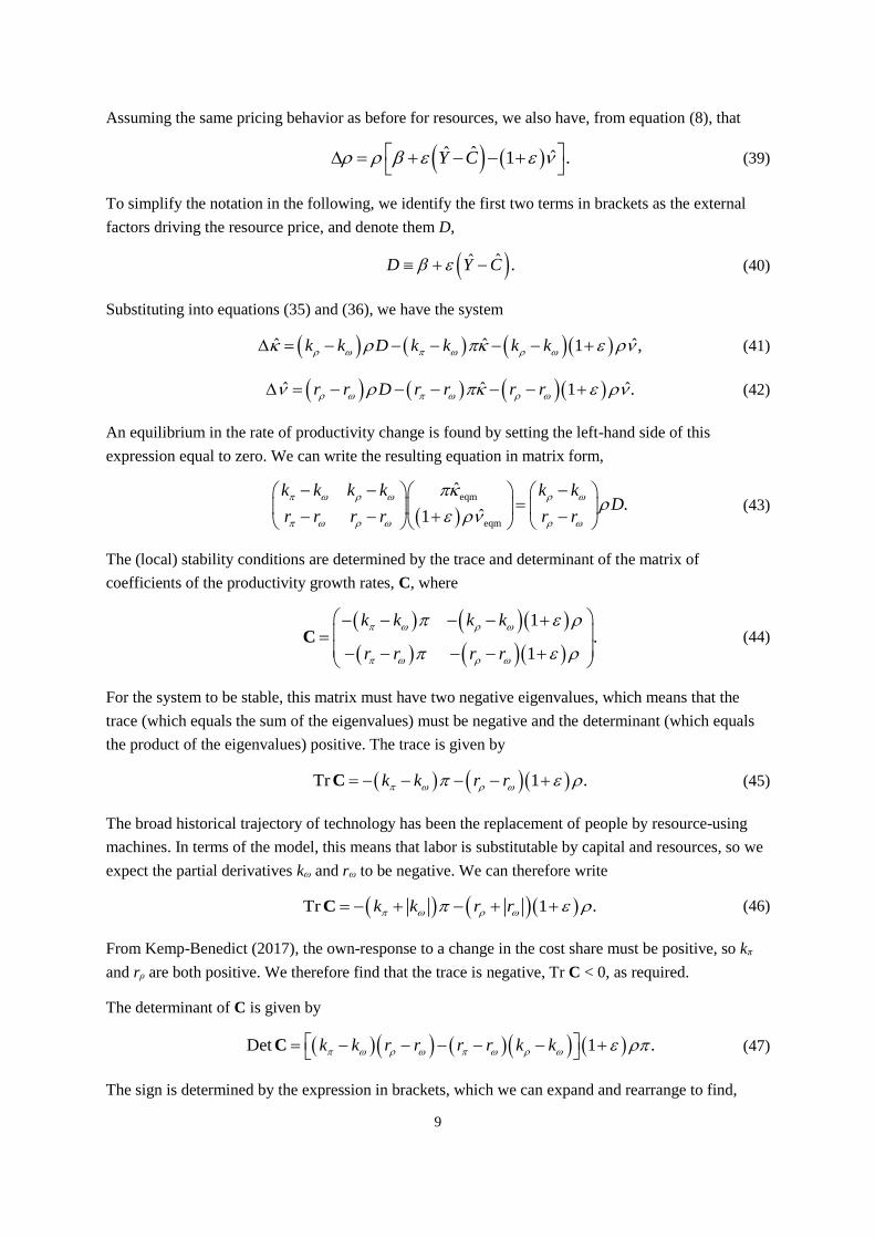
Assuming the same pricing behavior as before for resources, we also have, from equation (8), that
ˆˆ ˆ1 .Y C
(39)
To simplify the notation in the following, we identify the first two terms in brackets as the external
factors driving the resource price, and denote them D,
ˆˆ .D Y C (40)
Substituting into equations (35) and (36), we have the system
ˆ ˆ ˆ1 ,k k D k k k k (41)
ˆ ˆ ˆ1 .r r D r r r r (42)
An equilibrium in the rate of productivity change is found by setting the left-hand side of this
expression equal to zero. We can write the resulting equation in matrix form,
eqm
eqm
ˆ.
ˆ1
k k k k k kD
r r r r r r
(43)
The (local) stability conditions are determined by the trace and determinant of the matrix of
coefficients of the productivity growth rates, C, where
1.
1
k k k k
r r r r
C (44)
For the system to be stable, this matrix must have two negative eigenvalues, which means that the
trace (which equals the sum of the eigenvalues) must be negative and the determinant (which equals
the product of the eigenvalues) positive. The trace is given by
Tr 1 .k k r r C (45)
The broad historical trajectory of technology has been the replacement of people by resource-using
machines. In terms of the model, this means that labor is substitutable by capital and resources, so we
expect the partial derivatives kω and rω to be negative. We can therefore write
Tr 1 .k k r r C (46)
From Kemp-Benedict (2017), the own-response to a change in the cost share must be positive, so kπ
and rρ are both positive. We therefore find that the trace is negative, Tr C < 0, as required.
The determinant of C is given by
Det 1 .k k r r r r k k C (47)
The sign is determined by the expression in brackets, which we can expand and rearrange to find,

10
.k k r r r r k k k r r k k k r r r k (48)
In this expression, we have again assumed that labor is substitutable with capital and resources. The
first term in parentheses on the right-hand side is nonnegative because of an inequality that applies to
positive semi-definite matrices,
, .r k k r (49)
As discussed in Kemp-Benedict (2017), at most one of the remaining terms can in principle be
negative, which can occur only if capital and resources are complements. Even if one of the terms is
negative, it may still not be of sufficient magnitude to overcome the other, positive, terms, but it does
raise the possibility. The final term could plausibly be negative under conditions in which the resource
cost share is very low, wage costs are high, and resource-intensive capital tends to replace labor. In
that case the response of resource intensity to the profit share, rπ, could exceed the own-response, rρ.
However, we do not expect that condition to persist, as it would drive resource costs progressively
higher, until the cost share is no longer small. Once the cost share has risen sufficiently large, we
expect firms to use more resource-efficient machinery and otherwise seek to reduce their resource
costs. Thus, in mature economies we expect the determinant to be positive, Det C > 0.
Because the trace of C is negative, and the determinant is expected to be positive in mature
economies, we conclude that the equilibrium defined by equation (43) is stable.
Next, we consider cost shares. From equation (38), the equilibrium rate of change of the profit share is
eqm eqmˆ . (50)
The equilibrium rate of change of the resource share is, from equation (39) and the definition of D in
equation (40),
eqm eqmˆ1 .D (51)
Substituting these expressions into the equilibrium condition in equation (43) and cancelling a
common term on each side, we find
eqm
eqm
0.k k k k
r r r r
(52)
This equation implies constant cost shares, Δπeqm = Δρeqm = 0, unless the determinant of the matrix is
equal to zero. It is straightforward to show that the determinant of this matrix is the expression in
brackets in equation (47) for Det C. That is, this determinant can be zero only if Det C is zero. But we
have already argued that Det C should be positive. We therefore conclude that, at equilibrium, the
cost shares are not changing.
In the general equilibrium two-sector model, we recover the same equilibrium condition as in the
partial-equilibrium two-sector model. In addition, under target-return pricing, a constant resource
share and steady rate of resource productivity growth is accompanied by a steady profit share and
constant capital productivity.

11
5 Economic growth with and without resource constraints
With the two-sector model, in either the partial or full equilibrium case, the equilibrium rate of
productivity change satisfies equation (10), repeated here for convenience,
eqmˆˆˆ .
1 1Y C
(53)
We can characterize the price response of resource costs in the two cases in terms of the elasticity, ε,
with
0, resource abundant case,
, resource constrained case.
(54)
We then have
eqm
, resource abundant case,ˆ
ˆˆ , resource constrained case.Y C
(55)
The direction of causality in the resource abundant case is from economic growth to resource use.
This is the causal structure behind the environmental Kuznets curve (EKC) hypothesis. Our basic
result is that we should not expect absolute decoupling, with the implication that we should not expect
an EKC. Absolute decoupling can be stimulated over the short run if the supply price curve shifts
abruptly or during a structural transition toward sectors with lower resource intensity. However, in
either case the fall in resource intensity will not last. When the supply price curve stops shifting, the
productivity growth rate falls below the GDP growth rate, while a structural shift will eventually end,
leading at best to a sideways-s curve, first rising, then falling, and then rising again. These
conclusions appear consistent with the empirical literature, which has found no robust evidence for an
EKC (Stern 2004).
The resource constrained case corresponds to the conditions of Jevons’ paradox. Here, the causality is
reversed relative to the resource abundant case, which we express by moving the GDP growth rate to
the left-hand side of the equation,
eqmˆˆ ˆ .Y C (56)
Reading causality from the right-hand side of this equation to the left-hand side, GDP growth is
limited by the rate at which resource capacity can be expanded or resource productivity increased.
The equilibrium level of resource productivity growth should here be interpreted as the maximum
technically feasible rate. This is, effectively, Jevons’ paradox: when new resources are made
available, or the efficiency with which existing resources are used increases, output increases so as to
take advantage of the new capacity.
Both the resource abundant and resource constrained cases can be expressed in terms of a post-
Keynesian Leontief production function. In standard post-Keynesian theory, output can be either
capital or labor-constrained. With the possibility for limited natural resources, the production function
is,

12
min , , .Y K L C (57)
When resources are abundant, and there is excess labor, GDP growth is constrained by the pace of
capital accumulation. If labor is not abundant, as in a mature industrial economy, GDP growth can be
limited by the growth in labor productivity as well as the rate of capital accumulation. In a resource-
constrained economy, output can only grow as fast as resource capacity or resource productivity; this
is the condition expressed by equation (56). Resource constraints characterized the young industrial
economy that Jevons described. We may be entering such an era again, reflected in what Galbraith
(2014, 108) calls the “choke-chain effect”. The economy has free rein within the limits placed by
resource availability, but is sharply curtailed when it reaches the limits.
6 Stimulating absolute decoupling
The central result of this paper is essentially negative: unless resource supply is completely inelastic,
we cannot expect sustained absolute decoupling, because the search for profitable innovation does not
bring resource productivity growth above the rate of GDP growth. However, equation (55) suggests a
way to stimulate absolute decoupling through policy. The goal of the policy would be to continually
raise unit resource prices, as reflected in the parameter β. Given a target dematerialization rate, m,
where
ˆ ,R m (58)
the resource supply price schedule must shift vertically at a rate β*, where
* ˆ .Y m (59)
Whether the dematerialization target can in fact be reached depends on the underlying physical
processes. Human societies, including the economies embedded within them, require a steady flow of
energy and materials, and produce wastes. Some energy and materials sources are fully renewable, so
the only energy input is from the sun; some materials, such as steel, can be recycled with high
efficiency. But some materials are very difficult to substitute (Ayres 2007), while today’s renewable
technologies (such as biofuels) consume non-renewable inputs (such as synthetic fertilizers).
Dematerialization then involves questions of substitution (renewable energy sources, bio-based
materials) as well as more effective use of the existing inputs.
Technical studies typically show large potential for improving resource efficiency (e.g., for energy:
Nadel, Shipley, and Elliott 2004). For the purposes of this paper, we presume that substantial
dematerialization can occur over a policy-relevant time horizon, but for economic reasons it has not.
In this case, equation (59) can guide resource pricing policy. For example, a resource tax could be
assessed, which would steadily grow over time at a pace benchmarked to the realized rate of GDP
growth. The tax revenues could be allocated in such a way as to ease the transition, for example
through a revenue-neutral redistribution.
The proposal for stimulating decoupling as suggested by the model in this paper can be contrasted
with conventional neoclassical theory, in which resources may be priced to correct an externality; that
is, a social cost that is not borne directly by the participants in a market exchange. From this
standpoint, the goal of policy is to internalize the externality by “getting the prices right”. In contrast,

13
under a policy consistent with equation (59), the price is always changing, so there is no “right price”
to which to adjust. Rather, the goal is to continually push resource costs up, even as firms drive them
down through technological innovation. The policy target is specified on a purely physical basis,
through the dematerialization target rate m.
The difference reflects divergent approaches to policy analysis. In conventional policy analysis, the
policy goal is to maximize aggregate welfare. Markets are seen as the best tool for the job (on the
strength of the “welfare theorems”), so if a market is absent or incomplete then one should be
introduced. Despite developments within neoclassical theory itself that invalidate the premises behind
the welfare theorems, they remain the guiding principles of practical economic policy analysis
(Gowdy and Erickson 2005). In practice, an optimal solution is sought using cost-benefit analysis,
which brings the problems identified by Gowdy and Erickson to the surface. As applied to
environmental policy, cost-benefit analysis suffers from: implausible and inappropriate valuations;
application of discounting outside its domain of validity; problems of fairness and morality when
making decisions based on aggregate monetized costs and benefits; and the subtle introduction of
values into a putatively objective process (Ackerman and Heinzerling 2002, 1563).
In this paper we take a different approach. Taking it as given that the political and legal spheres are
the appropriate arenas for normative debate, an economic analysis should take as inputs the goals
emerging from those debates. The purpose of the economic analysis is to answer whether the goal can
be reached through a specifically economic mechanism. If it can, the proposed mechanism can be
assessed against other proposals on the table. That assessment nearly always involves a political
calculation. The subsequent policy design and implementation is then a combination of more
localized policy decisions, including public consultation, and technical exercises. The process might
be guided by the “four E’s” of traditional public administration: economy, efficiency, effectiveness,
and equity. Aside from “effectiveness”, each of these criteria has been given multiple definitions, and
the emphasis has shifted over time (Howlett, Mukherjee, and Rayner 2015), with equity a relatively
recent entrant (Norman-Major 2011). Nevertheless, some broad regularities can be discerned.
Economy is generally taken to mean that staff and budget are aligned with available resources, while
policy goals are achieved without undue expense. Efficiency refers to implementation, in that the
number, composition and sequencing of policy instruments is consonant with the intended goal.
Effectiveness means the proposed policy achieves its goal. Equity addresses the perceived fairness and
justice of outcomes, as well as inclusive policy design.
To the extent that the theory in this paper reflects the real world, the policy suggested by equation (59)
should be effective in driving decoupling at a rate specified in policy commitments. Further, it has the
potential to be both economic and equitable. In broad outline, the policy could be implemented by
assessing a revenue neutral tax at the wellhead (or at port of entry). The tax would be applied directly
in only a few sectors, while the revenues could be distributed through a social dividend (Boyce and
Riddle 2007) or similar scheme intended to be both fair and transparent. The proposed policy also has
the potential to be efficient, in that, although it covers nearly all sectors of the economy, it requires
only two policy instruments: a tax whose rate is the sum of a target rate of dematerialization and
recent (e.g., previous quarter) estimated real GDP growth; and a revenue distribution policy.
14
Climate mitigation policy in practice is informed by neoclassical theory, and often includes a carbon
price, whether as a tax, the price of an emissions credit in an emissions trading scheme, or an
“internal” price used by government or business for planning purposes. The World Bank State and
Trends of Carbon Pricing 2016 (World Bank, Ecofys, and Vivid Economics 2016, 56) lists three
sources for internal prices: estimates of the social cost of carbon (SCC); estimated marginal abatement
cost; or current or anticipated market values of emissions allowances. The first and third approaches
should, according to conventional analysis, yield values similar to each other, but the internal prices
reported in the World Bank report varied over three orders of magnitude. Experience with SCC
estimates (Tol 2011) offers one explanation. The SCC approach is closest in spirit to conventional
theory, in that it is an estimate of the marginal cost or benefit that ought to be internalized. However,
SCC estimates are challenging (Metcalf 2008); there are substantial uncertainties in the size of some
impacts, and when these are taken into account, cost estimates can vary over a wide range (Ackerman
and Stanton 2012). Conventional pricing theory faces a further challenge. Each of the three
approaches listed above should generate prices that rise over time as greenhouse gas concentrations
and global average temperatures rise, yet the European Emissions Trading Scheme (EU ETS) saw
prices fall substantially in recent years, part of a longer downward trend with large fluctuations
around the trend (Meadows, Slingenberg, and Zapfel 2015, fig. 2.5).
Thus, while existing pricing schemes may appear similar to the policy suggested by the theory in this
paper, the similarities are superficial. No estimate of social cost or market-clearing price informs
equation (59), and it does not rely on detailed calculation of marginal abatement costs. Rather, a
physically-based mitigation goal determines m, which then determines β*. In practice, countries
specify their climate mitigation goals through politically-negotiated and physically-based targets, the
nationally determined contributions (NDCs) arising from the Paris climate agreement. The NDCs
have a direct analogue in equation (59) in the dematerialization target rate m.
7 Conclusions
The prospects for sustainability depend crucially on the ability to decouple material throughput from
economic value. As this has not happened in the past, one may doubt whether it is possible in the
future. In this paper we provide an explanation for why decoupling has not yet occurred, based on two
assumptions – that resource prices rise with demand and that the pace of resource productivity
improvement rises with the resource cost share.
The theory presented in this paper suggests that when resources are comparatively abundant, relative
decoupling may occur, but absolute decoupling will not, except during periods when resource costs
are rising faster than GDP. When resources are constrained, GDP growth is determined by the rate of
expansion of resource supply and the technically feasible rate of resource productivity growth. In the
latter half of the 19th century, when Jevons (1865) wrote The Coal Question, coal was a constraining
resource, so any advances in extractive technology or efficiency of use led, paradoxically, to even
greater resource use, rather than less.
We may be entering a new resource-constrained era, but even if we are, we are not bringing carbon-
intensive energy consumption down fast enough to meet globally-agreed carbon mitigation goals
(UNEP 2016). The theory presented here suggests that absolute decoupling can only be driven by a

15
sufficiently rapidly rising resource price. By ensuring a steady and predictable rise in resource costs
that exceeds the GDP growth rate, firms are encouraged to continually raise resource productivity at a
rate sufficient to absolutely decoupling resource use from GDP. The proposed policy is more
predictable than that suggested by conventional theory, which urges that a carbon price be set at a
periodically updated social cost of carbon that reflects the damages inflicted by a marginal unit of
carbon emissions. It is also more directly applicable to policy implementation, as the policy
instrument directly incorporates the physical goal that the policy is meant to address.
References
Acemoglu, Daron, Philippe Aghion, Leonardo Bursztyn, and David Hemous. 2012. “The
Environment and Directed Technical Change.” American Economic Review 102 (1): 131–66.
doi:10.1257/aer.102.1.131.
Ackerman, Frank, and Lisa Heinzerling. 2002. “Pricing the Priceless: Cost-Benefit Analysis of
Environmental Protection.” University of Pennsylvania Law Review 150 (5): 1553–84.
doi:10.2307/3312947.
Ackerman, Frank, and Elizabeth A. Stanton. 2012. “Climate Risks and Carbon Prices: Revising the
Social Cost of Carbon.” Economics: The Open-Access, Open-Assessment E-Journal 6 (2012–
10): 1. doi:10.5018/economics-ejournal.ja.2012-10.
Alcott, Blake. 2005. “Jevons’ Paradox.” Ecological Economics 54 (1): 9–21.
doi:10.1016/j.ecolecon.2005.03.020.
Auty, Richard. 1985. “Materials Intensity of GDP: Research Issues on the Measurement and
Explanation of Change.” Resources Policy 11 (4): 275–83. doi:10.1016/0301-4207(85)90045-
5.
Ayres, Robert U. 2007. “On the Practical Limits to Substitution.” Ecological Economics 61 (1): 115–
28. doi:10.1016/j.ecolecon.2006.02.011.
Ayres, Robert U., and Jeroen C.J.M. van den Bergh. 2005. “A Theory of Economic Growth with
Material/Energy Resources and Dematerialization: Interaction of Three Growth
Mechanisms.” Ecological Economics 55 (1): 96–118. doi:10.1016/j.ecolecon.2004.07.023.
Ayres, Robert U., and Benjamin Warr. 2009. The Economic Growth Engine: How Energy and Work
Drive Material Prosperity. Cheltenham, UK: Edward Elgar Publishing.
Bernardini, Oliviero, and Riccardo Galli. 1993. “Dematerialization: Long-Term Trends in the
Intensity of Use of Materials and Energy.” Futures 25 (4): 431–48. doi:10.1016/0016-
3287(93)90005-E.
Boyce, James K., and Matthew Riddle. 2007. “Cap and Dividend: How to Curb Global Warming
While Protecting the Incomes of American Families.” Working Paper 150. Working Paper.
Amherst College, Amherst, MA: Political Economy Research Institute.
http://scholarworks.umass.edu/peri_workingpapers/108/.
Cogoy, Mario. 2004. “Dematerialisation, Time Allocation, and the Service Economy.” Structural
Change and Economic Dynamics 15 (2): 165–81. doi:10.1016/S0954-349X(03)00025-0.
Coutts, Ken, and Neville Norman. 2013. “Post-Keynesian Approaches to Industrial Pricing.” In The
Oxford Handbook of Post-Keynesian Economics, Volume 1: Theory and Origins, edited by
G.C. Harcourt and Peter Kriesler.

16
Cullenward, Danny, and Jonathan G. Koomey. 2016. “A Critique of Saunders’ ‘Historical Evidence
for Energy Efficiency Rebound in 30 US Sectors.’” Technological Forecasting and Social
Change 103 (February): 203–13. doi:10.1016/j.techfore.2015.08.007.
Dinda, Soumyananda. 2004. “Environmental Kuznets Curve Hypothesis: A Survey.” Ecological
Economics 49 (4): 431–55. doi:10.1016/j.ecolecon.2004.02.011.
Duménil, Gérard, and Dominique Lévy. 1995. “A Stochastic Model of Technical Change: An
Application to the US Economy (1869–1989).” Metroeconomica 46 (3): 213–245.
doi:10.1111/j.1467-999X.1995.tb00380.x.
Foley, Duncan K. 2003. Unholy Trinity: Labor, Capital, and Land in the New Economy. London;
New York: Routledge.
Galbraith, James K. 2014. The End of Normal: The Great Crisis and the Future of Growth. New
York, NY, US: Simon & Schuster. http://books.simonandschuster.com/The-End-of-
Normal/James-K-Galbraith/9781451644937/browse_inside.
Gowdy, John, and Jon D. Erickson. 2005. “The Approach of Ecological Economics.” Cambridge
Journal of Economics 29 (2): 207–22. doi:10.1093/cje/bei033.
Hicks, J.R. 1932. The Theory of Wages. London: MacMillan and Company Limited.
Howlett, Michael, Ishani Mukherjee, and Jeremy Rayner. 2015. “Chapter 10: Designing Effective
Programs.” In Handbook of Public Administration, edited by Robert K. Christensen and
James L. Perry, 3rd ed. San Francisco, CA, US: Jossey-Bass.
http://proquest.safaribooksonline.com.ezproxy.library.tufts.edu/9781119004325.
Jevons, William Stanley. 1865. The Coal Question: An Inquiry Concerning the Progress of the
Nation, and the Probable Exhaustion of Our Coal-Mines. London and Cambridge, UK:
Macmillan and Co.
Kalecki, Michal. 1969. Theory of Economic Dynamics: An Essay on Cyclical and Lon-Run Changes
in Capitalist Economy. New York, NY, US: Augustus M. Kelly.
Kemp-Benedict, Eric. 2017. “Biased Technological Change and Kaldor’s Stylized Facts.” Working
Paper 76803. MPRA Paper. Munich, Germany: Munich Personal RePEc Archive.
Khazzoom, J. Daniel. 1980. “Economic Implications of Mandated Efficiency in Standards for
Household Appliances.” The Energy Journal 1 (4): 21–40.
http://www.jstor.org.ezproxy.library.tufts.edu/stable/41321476.
Kijima, Masaaki, Katsumasa Nishide, and Atsuyuki Ohyama. 2010. “Economic Models for the
Environmental Kuznets Curve: A Survey.” Journal of Economic Dynamics and Control 34
(7): 1187–1201. doi:10.1016/j.jedc.2010.03.010.
Kriesler, Peter. 1988. “Kalecki’s Pricing Theory Revisited.” Journal of Post Keynesian Economics 11
(1): 108–30. http://www.jstor.org/stable/4538119.
Kumar, Surender, and Shunsuke Managi. 2009. “Energy Price-Induced and Exogenous Technological
Change: Assessing the Economic and Environmental Outcomes.” Resource and Energy
Economics 31 (4): 334–53. doi:10.1016/j.reseneeco.2009.05.001.
Lee, Frederic S. 1999. Post Keynesian Price Theory. Cambridge University Press.
McGlade, Christophe, and Paul Ekins. 2015. “The Geographical Distribution of Fossil Fuels Unused
When Limiting Global Warming to 2 °C.” Nature 517 (7533): 187–90.
doi:10.1038/nature14016.

17
Meadows, Damien, Yvon Slingenberg, and Peter Zapfel. 2015. “EU ETS: Pricing Carbon to Drive
Cost-Effective Reductions across Europe.” In EU Climate Policy Explained, edited by Jos
Delbeke and Peter Vis, 29–60. London ; New York, NY: Routledge.
Metcalf, Gilbert E. 2008. “Designing a Carbon Tax to Reduce U.S. Greenhouse Gas Emissions.”
Review of Environmental Economics and Policy, November, ren015.
doi:10.1093/reep/ren015.
Metcalf, Gilbert E., and David Weisbach. 2009. “The Design of a Carbon Tax.” Harvard
Environmental Law Review 33: 499–556.
Nadel, Steven, Anna Shipley, and R. Neal Elliott. 2004. “The Technical, Economic and Achievable
Potential for Energy-Efficiency in the US–A Meta-Analysis of Recent Studies.” In
Proceedings of the 2004 ACEEE Summer Study on Energy Efficiency in Buildings, 8–215.
http://www.regie-energie.qc.ca/audiences/3584-05/Audience3584/PiecesDeposees/C-10-6-
ROEE_Eng1-ACEEE-Potential-Meta-Analysis_3584_22fev06.pdf.
Nelson, Richard R., and Sidney G. Winter. 1982. An Evolutionary Theory of Economic Change.
Cambridge, Mass.: Belknap Press of Harvard University Press.
Norman-Major, Kristen. 2011. “Balancing the Four Es; or Can We Achieve Equity for Social Equity
in Public Administration?” Journal of Public Affairs Education 17 (2): 233–52.
http://www.jstor.org.ezproxy.library.tufts.edu/stable/23036113.
Sorrell, Steve. 2009. “Jevons’ Paradox Revisited: The Evidence for Backfire from Improved Energy
Efficiency.” Energy Policy 37 (4): 1456–69. doi:10.1016/j.enpol.2008.12.003.
Stern, David I. 2004. “The Rise and Fall of the Environmental Kuznets Curve.” World Development
32 (8): 1419–39. doi:10.1016/j.worlddev.2004.03.004.
Tol, Richard S. J. 2011. “The Social Cost of Carbon.” Annual Review of Resource Economics 3 (1):
419–43. doi:10.1146/annurev-resource-083110-120028.
UN General Assembly. 2015. “Transforming Our World: The 2030 Agenda for Sustainable
Development.” Resolution A/RES/70/1. Resolution. United Nations.
http://www.un.org/ga/search/view_doc.asp?symbol=A/RES/70/1&Lang=E.
UNEP. 2016. The Emissions Gap Report 2016: A UNEP Synthesis Report. Nairobi, Kenya: United
Nations Environment Programme.
Wagner, Martin. 2008. “The Carbon Kuznets Curve: A Cloudy Picture Emitted by Bad
Econometrics?” Resource and Energy Economics 30 (3): 388–408.
doi:10.1016/j.reseneeco.2007.11.001.
Warr, Benjamin, and Robert U. Ayres. 2012. “Useful Work and Information as Drivers of Economic
Growth.” Ecological Economics 73 (January): 93–102. doi:10.1016/j.ecolecon.2011.09.006.
World Bank, Ecofys, and Vivid Economics. 2016. “State and Trends of Carbon Pricing 2016.”
Washington, DC, US: The World Bank.
https://openknowledge.worldbank.org/handle/10986/25160.