Demand Shocks, Capacity Coordination and Industry Performance:

Lessons from an Economic Laboratory

Kyle Hampton ∗ and Katerina Sherstyuk†‡

Abstract

Antitrust exemptions granted to businesses under extenuating circumstances are often jus-tified by the argument that they benefit the public by helping producers adjust to otherwisedifficult economic circumstances. Such exemptions may allow firms to coordinate their capac-ities, as was the case of post-September 11, 2001 antitrust immunity granted to Aloha andHawaiian Airlines. We conduct economic laboratory experiments to determine the effects ofexplicit capacity coordination on oligopoly firms’ abilities to adjust to negative demand shocksand on industry prices. The results suggest that capacity coordination speeds the adjustmentprocess, but also has a clear pro-collusive effect on firm behavior.

∗Department of Economics, University of Alaska Anchorage. Email: afkh2@uaa.alaska.edu†Corresponding author. Department of Economics, University of Hawaii at Manoa. Email: katyas@hawaii.edu‡We would like to thank James Mak for many motivating discussions and useful feedback, and Mark Armstrong,

two anonymous referees, Roger Blair, Tim Cason, Tim Halliday, Rene Kamita, Andreas Leibbrandt, Charles Plott,Bart Wilson, participants of the 2007 Economic Science Association meetings in Tucson, Arizona, 2008 WesternEconomic Association International meetings in Honolulu, Hawaii, and seminar participants at the University ofAlaska Anchorage, University of Hawaii at Manoa and Florida State University for their valuable comments.

1

1 Introduction

It is not unusual for firms in distressed industries to seek government assistance. In industries

experiencing a sharp and sudden decrease in demand, firms may request help in coordinating a

capacity reduction. In the years following World War II, many of Japan’s large industrial firms

faced the task of reducing their wartime capacity and encountered the difficult strategic situation

of making unilateral reductions. This prompted the creation of an industrial policy to facilitate the

structured and balanced reduction of capacity across all firms in the industry (Peck et al., 1987).

In Europe, competition law may allow firms in a distressed industry to form “crisis cartels,” or

agreements to systematically restrict output or reduce capacity in response to a crisis in the indus-

try. Indeed, crisis cartels were formed in the European synthetic fiber industry in the 1980’s and in

the Dutch brick industry in the 1990’s. In each case, the agreements provided for specific capacity

reductions by individual producers in response to structural excess capacities in the corresponding

industries (Fiebig, 1999; Simpson, 2004). A similar attempt to balance capacity reduction in the

face of decreased demand took place recently in the United States. In 2002, the U.S. Department

of Transportation granted antitrust immunity to Aloha and Hawaiian Airlines in order to facilitate

a bilateral reduction in inter-island flight capacity in Hawaii after a reduction in demand following

the September 11, 2001 terrorist attacks. Beyond merely permitting the two companies to coordi-

nate their capacity reduction, the immunity agreement created a mechanism for revenue transfers

designed to punish either company if they deviated from the agreed-upon capacity reduction.1

In this study, we use economic experiments to examine the effects of capacity coordination

on industry performance in response to a negative demand shock. One could argue that explicit

coordination by firms is critical in the face of a challenging reduction in demand. But coordi-

nation may also encourage anti-competitive behavior by participating firms. Proponents of the

Aloha-Hawaiian antitrust immunity agreement argued that it was impossible for the two airlines to

unilaterally reduce their capacity enough to avoid bankruptcy in reaction to a post-9/11 reduction

in air travel (Aloha Airlines and Hawaiian Airlines, 2002).2 The U.S. Department of Justice, in

opposing the anti-trust exemption, claimed that the agreement would undermine consumer welfare

by allowing the airlines market power sufficient to reduce service and raise prices well above the

competitive level. Inter-island airfares did rise dramatically following the inception of the agree-

ment in 2002 (Blair et al., 2007; Kamita, 2010).3 Yet, it is difficult to conclude, based on mere field

data analysis, whether these price increases were necessarily due to capacity coordination. Further,

1An earlier case of coordinated capacity reduction in the U.S. airline industry took place in 1971, when the CivilAeronautics Board approved a capacity limitations agreement among three airline carriers (Eads, 1974).

2Aloha Airlines declared bankruptcy and went out of business in Spring 2008 despite the immunity agreement.Arguably, however, the primary reason for Aloha’s going out of business was entry by a competitor airline go!, notthe 2001 demand shock.

3Kamita (2010) reports not only that prices rose during the period of coordination, but that they remained highuntil the entry of a new competitor, two and a half years after the antitrust immunity expired.

2

it is difficult to determine whether or not explicit coordination was necessary for the firms to re-

duce their capacity in the face of decreased demand. Experimental methods have the advantage

of permitting researchers to isolate effects of specific institutional features (Plott, 1989). Economic

experiments have proven increasingly useful both in detecting anti-competitive effects of various

industry practices (Grether and Plott, 1984; Offerman and Potters, 2006; Deck and Wilson, 2008),

and in evaluating techniques used by antitrust authorities to hinder collusion (Apesteguia et al.,

2007; Hinloopen and Soetevent, 2008).

There are theoretical and empirical arguments in the literature both for and against antitrust

authorities allowing explicit capacity coordination. Capacity coordination in response to an unex-

pected negative demand shock in the airline industry may be justified by its cost structure, which

includes large sunk costs (e.g., the cost of acquiring an aircraft) and large costs that can be avoided

by not flying the aircraft but become fixed once the flight is scheduled (e.g., the cost for fuel and

crew). As the scheduling of flights takes place before the seats are booked, the airlines run the risk

of not covering their total costs unless they can predict the demand accurately and are able to set

prices at levels above their marginal costs. This accounts for the necessity of above-marginal-cost

pricing by firms in industries with large sunk and avoidable costs (Sjostrom, 1989; Durham et al,

2004; see also Van Boening and Wilcox, 1996). Kreps and Sheinkman (1983) develop a two-stage

oligopoly model where firms first set their capacities, and then engage in price competition. They

demonstrate that in this setting, Cournot-level above-marginal-cost pricing will emerge even with-

out explicit capacity coordination, provided that the firms observe each other’s capacity choices

prior to setting their prices. This model appears appropriate for the airline industry, where ca-

pacities (flight schedules) are set before tickets are sold and companies may observe each other’s

capacities though publicly announced flight schedules. However, firms’ knowledge of demand is an

essential assumption in the Kreps and Scheinkman model. An unexpected demand shock may lead

to over-investment in capacity and losses either from unsold seats, or from marginal cost pricing.4

Further, it may be unrealistic to expect firms to adjust to new demand conditions instantaneously.

If explicit capacity coordination allows firms to adjust to these new conditions faster, then it may

help the firms avoid losses and stay in business. This could yield an argument for the antitrust

exemption, provided that welfare gains from doing so outweigh potential costs to consumers.

The argument against explicit capacity coordination is backed by a large theoretical, empirical

and experimental literature on collusion in oligopoly. Both game-theoretical (Tirole, 1988) and

experimental research (Fouraker and Siegel, 1963; Dufwenberg and Gneezy, 2000; Huck et al.,

2004) indicates that industries with a small number of firms with symmetric cost structures, who

interact repeatedly under known and stable demand conditions, are prone to tacit collusion in

4If the demand shock is unanticipated, then capacities set before the shock become exogenous. Depending onthe level of capacity set, the subsequent price competition may result in either marginal cost pricing, or in priceinstability due to the non-existence of a pure strategy equilibrium (Osborne and Pitchik, 1986; Kruse et al., 1994).

3

the form of above-competitive pricing.5 Empirical evidence of collusion in oligopolies, especially

duopolies, is also quite rich (Rees, 1993; Levenstein and Suslow, 2006). Though it is plausible

that duopolists in an industry with stable demand could achieve above-competitive pricing, an

unexpected negative demand shock would constitute a major challenge (Levenstein and Suslow,

2006; Staiger and Wolak, 1992). An antitrust immunity agreement that allows firms to explicitly

coordinate and enforce capacity reductions could help firms establish or re-establish collusive pricing

in a new environment and in this way have a detrimental effect on consumer welfare.

There are several cases detailed in the literature where government authorities have uninten-

tionally helped firms to collude (Albaek et al., 1997); and other cases where explicit coordination

helped firms to avoid bankruptcy (Sjostrom, 1989). In this view, consideration of the effect of ca-

pacity coordination on competition and overall outcomes in an industry experiencing an unexpected

demand shocks is of particular interest.

In this article we report on an economic laboratory experiment that was conducted to evaluate

effects of capacity coordination on oligopolistic industry performance. We recreate the Kreps and

Sheinkman (1983) two-stage capacity and price setting duopoly game in the economic laboratory,

but with repeated play in order to model firms who interact with each other for a long time under

known and stable demand conditions. This allows us to establish, as a baseline, whether firms

are likely to engage in above-marginal-cost pricing even without explicit coordination. We then

institute a negative demand shock halfway through each experimental session, in order to investigate

its effect on firm behavior. By then varying regulatory regimes after the demand shock (allowing

or not allowing capacity coordination, and enforcing or not enforcing the agreed-upon capacity

restrictions), we further examine how different capacity coordination regimes affect post-shock

industry outcomes. This method allows us to evaluate whether capacity coordination agreements

are likely to facilitate capacity reduction and to what extent these agreements are anti-competitive.

Davis (1999) and Muren (2000) study experimental triopoly markets in repeated settings in the

framework of the Kreps and Sheinkman (1983) two-stage capacity and price setting game. Davis

finds that capacity pre-setting raises prices and reduces capacity, though with substantial variation

across markets. Muren reports that capacity choices for inexperienced subjects are higher (more

competitive) than the Kreps and Sheinkman (1983) model predicts. Goodwin and Mestelman

(2010) also report that inexperienced subjects over-invest in capacities in Kreps and Sheinkman

duopolies, but that capacities converge to the Cournot prediction as subjects gain experience.

However, these articles do not consider demand changes, which is the main focus of our study.

Other experimental studies analyze the ability of market institutions to adjust to supply and

demand shifts (Williams and Smith, 1984; Davis et al., 1993). Still others consider the effects

5At the time of September 11th attacks, Hawaii’s inter-island airline industry was largely dominated by two mainproviders, Aloha and Hawaiian airlines, who had symmetric cost structures, near equal market shares, providedhomogeneous product, and had been operating in this industry for a long time (Blair et al., 2007; Kamita, 2010).

4

of certain industrial practices or government programs on market outcomes (Grether and Plott,

1984; Hinloopen and Soetevent, 2008), but under stable economic conditions. Many experiments

investigate collusion in a variety of market settings, but only a few (e.g., Brown et. al., 2009)

explore the robustness of established collusive practices under changing conditions. The unique

contribution of this article is two-fold. First, we study the effect of a negative demand shock on

firms’ abilities to sustain above-marginal-cost pricing in the Kreps and Sheinkman (1983) two-

stage capacity and price competition framework. This setting is arguably more complex than

simple quantity- or price- oligopoly competition; therefore it may be more challenging for firms to

adjust to changes in demand. Second, we focus on the effects of regulatory measures that may

be instituted in response to sudden negative changes in economic conditions. Our experimental

evidence adds to and complements the scarce empirical literature (e.g., Kamita 2010) on the effect

of capacity coordination on firms’ abilities to both reduce capacities and engage in tacit collusion.

Our key experimental findings are as follows. First, we observed that explicit capacity coordi-

nation helped firms quickly adjust their capacities when demand conditions changed. Yet, most

firms reduced capacity immediately after the demand shock even in markets where no explicit co-

ordination was allowed. The demand shock did not result in persistent losses or firm bankruptcies

in any of the markets.6 Second, we obtained strong evidence that in many experimental markets,

capacity coordination had a pronounced pro-collusive effect on firm behavior. Whereas prices fell

and remained low after the demand shock in markets without capacity coordination, prices quickly

recovered and even increased in markets with coordination. This is quite remarkable because, in

our experiment, sellers coordinated capacities in settings more restrictive than real-world capacity

negotiations. Under the 2002 Aloha-Hawaiian anti-trust exemption, representatives of both airlines

met every 30 days to agree on flight capacities for the next month; the meetings took place behind

closed doors, with apparently no direct oversight from the Attorney General’s office. Negotiations

in our experiment were not face-to-face; they were computer-mediated, and restricted to alternating

capacity proposals, with the additional ability, in some treatments, to engage in moderated online

chats. Third, we observed that whereas the ability to coordinate capacity levels had a significant

effect on reducing capacities and increasing prices immediately after the negotiations started, the

effect of explicit agreement enforcement became the most pronounced in later negotiations periods.

Finally, we find that supplementary free-style communication enhanced firm abilities to sustain ca-

pacity agreements and ultimately resulted in the highest share of perfectly collusive markets among

all institutions considered.

The rest of the article is organized as follows. Research objectives, design and procedures

are given in Section 2. Section 3 presents the results, and Section 4 concludes. Experimental

6In fact, the only two markets where the sellers experienced on-going losses and went bankrupt were in the treat-ments allowing for coordination; see Table 1. These losses were most likely due to the subjects’ lack of understandingof the market, rather than the demand shock, as the losses started and persisted in the periods before the shock.

5

instructions and other supplementary materials are given in the on-line appendix.

2 Research objectives and experimental design

The experiment is designed to explore the effects of capacity coordination in an oligopoly industry

experiencing a sudden negative demand shock. Specific research objectives are the following. First,

as a benchmark, we explore firms’ abilities to avoid excess capacities and achieve and sustain above-

marginal-cost pricing without explicit coordination in a repeated two-stage capacity-price-setting

duopoly. Second, we study the effects of a negative demand shock on industry outcomes in this

environment, and on producers’ abilities to adjust to the new demand conditions without explicit

coordination. Third, we examine the ability of several capacity coordination institutions to help

producers adjust to a negative demand shock. We compare the speed and the extent of capacity

reduction under each institution, and the effects of the institutions on firm profits as a proxy for

producer welfare. Finally, we investigate whether capacity coordination has a pro-collusive effect

on firm behavior, leading to higher industry prices.

Experimental Design The basic design mirrors the Kreps and Sheinkman (1983; hereafter KS

1983) two-stage capacity-price duopoly model, except similar to many market experiments, we add

a repeated setting as this is more appropriate in modeling most real-world oligopolies. Each market

is conducted as a series of trading periods in which two subjects in the roles of sellers compete to

sell units of a fictitious good to a simulated buyer with a known linear demand. In line with

KS (1983), the institution is a modified posted offer market, where subjects specify production

and observe the production level of their counterpart prior to setting a price in each period. The

capacity setting is simultaneous and - in the first part of each experimental session - is undertaken

without communication between the sellers. Sellers incur costs on each unit of capacity produced

regardless of how many units they actually sell. The capacities set by each seller are then revealed

to the other seller in the market, after which the sellers simultaneously and privately specify an

asking price for the goods they have produced. After that, the simulated buyer purchases units

from the sellers, buying from the lower priced seller first.7 At the end of each trading period, sales

and the corresponding profits or losses are reported to the sellers along with the posted price and

the sales of the other seller.

Parameters Each seller faces a constant marginal cost of 10 experimental dollars per unit and no

fixed costs. We abstract from a more realistic setting of large fixed costs and non-constant marginal

7The sales are determined exactly as in the KS (1983) model. We do not explore alternative models of advancedcapacity setting (Davidson and Deneckere, 1986; Moreno and Ubeda, 2006), as the KS model accurately describesthe real-world market setting we study: two producers with symmetric market shares and with some price-settingpower.

6

cost to focus on the issue of capacity coordination and its effect on the prices in a relatively simple

environment. Each seller makes their capacity and pricing decisions in light of a known continuous

linear demand function, which was set to be Q = 304− 4(p) for the first 21 trading periods.

In the 22nd period, a demand shock is induced by a decrease in the intercept of the demand

function. The post-shock demand that persists for the remainder of the session is then Q =

256− 4(p).

This decrease in demand occurs in the course of a period (referred to as the “shock period”)

after the capacity-setting stage has elapsed. Subjects are made aware of the change at that time

and post their price in light of the new demand information. Subjects are warned during the

instructions that a change in the demand is possible.

These supply and demand conditions imply a market price and quantity combination associated

with each of three plausible theoretical benchmarks: Bertrand equilibrium (which would imply

marginal cost pricing of $10 and outcomes identical to perfect competition); Cournot outcome

(as predicted by KS, 1983), and Monopoly outcome (which may be supported by repeated play

and possibly enhanced by explicit capacity coordination). The demand parameters are chosen

so that the pre-shock Cournot price ($32 experimental) is below the post-shock monopoly price

($37 experimental), allowing for the replication of the post-shock price increase observed after the

inception of the anti-trust exemption agreement between Aloha and Hawaiian airlines.

Treatments The experiment consists of four main treatments and two additional treatments.

The main treatments are designed to investigate the effects of capacity-coordination institutions

established in response to a negative demand shock. The additional treatments are added to

separate the effects of capacity coordination from the effects of demand shock, and consider markets

where coordination starts prior to the demand shock. We introduce the four main treatments

next. The additional treatments will be introduced and discussed later, in the subsection “Early

coordination and enforcement” of Section 3.

For the four main treatments, the before-shock trading periods are conducted identically under

all treatments, with no capacity coordination. The demand shock is then instituted in period 22,

followed by three transition periods (periods 22-24, which we call the “shock periods”) with no

coordination. This short span of shock periods allows us to assess whether the subjects attempt

to unilaterally adjust to the new demand conditions immediately after the shock before any co-

ordination takes place. Starting from period 25, we vary capacity coordination and enforcement

institutions across sessions, giving rise to four distinct treatments:

Treatment “No Negotiations, No Punishment” (NoNegNoPun). In this baseline treat-

ment, the demand shock is followed by 14-16 additional periods under the new demand conditions

with no explicit capacity coordination. The institution is the same as in the pre-shock periods.

7

Treatment “Negotiations, Punishment” (NegPun) is modeled after the 2002 Aloha -

Hawaiian airlines anti-trust exemption. Following the three shock periods, the capacity coordination

mechanism is imposed and persists for the remainder of the session. In an additional stage at the

beginning of each period, sellers negotiate and agree upon a capacity per seller prior to setting

own capacity. In the event that either seller chooses to produce more than the agreed amount

that period, the offender is penalized seven experimental dollars per unit produced over the agreed

capacity, an amount chosen to exceed any potential gains that might accrue to the seller who broke

the agreement. This penalty is transferred to the other seller. In the event that both exceed the

agreed upon amount, the penalty is accrued to each with the net balance determined by the relative

size of the divergence of each seller. This setting is designed to mimic the actual revenue transfer

clause of the Aloha-Hawaiian airlines agreement.8

The negotiation stage takes the form of a real-time bargaining session. Each seller can propose

a per-seller capacity. During this negotiation stage, a seller can change their proposal at any time

as many times as they wish. Each seller, seeing the current proposal of the other seller, can choose

to propose a different capacity, accept the proposal of the other seller, or do nothing at all. Upon

either seller accepting the proposal of the other, the negotiations end immediately and the sellers

proceed to the capacity-setting stage. If no proposal is accepted in the time allotted for negotiations

(90 seconds), there is no agreement in place for that period.

Treatment “Negotiations, No Punishment” (NegNoPun) is identical to the NegPun

treatment described above, except that there is no penalty for breaking the capacity agreement.

This treatment is designed to isolate the effects of the enforcement (in the form of the revenue

transfer clause) on the effectiveness of the agreement.

Treatment “Negotiations, No Punishment, Chat” (NegChat) replicates the Neg-

NoPun treatment but allows, in parallel with structured negotiations, free form communication

between the subjects in a chat window. This treatment is motivated by a large body of existing

literature on non-binding communication in experimental markets and games (Holt, 1995; Craw-

ford, 1998). It aims to investigate whether free-style non-binding communication could lead to

better coordination than the structured negotiations alone, and whether it may substitute for an

explicit punishment clause in promoting and maintaining capacity reductions. Chats are monitored

and subjects are warned not to discuss price in their chats, with the threat of removal from the

experiment if they do not comply.

Procedures 41 two-person markets were conducted under the four main treatments over the

course of 13 experimental sessions. Eight sessions were conducted at the University of Hawaii at

8The revenue transfer clause of the Aloha-Hawaiian agreement specified the penalty level at around 60-100% ofextra revenue from per unit deviation from the agreed capacity (Blair et. al., 2007). Accordingly, we set the penaltylevel at about 60% of possible per unit gain from deviation from the perfectly collusive monopoly outcome.

8

Manoa (UHM hereafter) and five sessions were conducted at the University of Alaska Anchor-

age (UAA hereafter). Table 1 provides a summary of the experimental sessions (both main and

additional treatments).

TABLE 1 AROUND HERE

Each session began with an oral reading of the instructions, a quiz confirming the subjects’ under-

standing of the instructions (both given in on-line Appendix A)9 and a trial period. The experiment

was computerized using the z-tree software (Fischbacher, 2007). Subjects were seated at visually

isolated computer terminals with communication limited to the experiment interface. In treatments

with capacity coordination, further instructions on coordination were given in unpaid trial period

25, which preceded the paid negotiations periods. A market typically consisted of 39 paid periods,

with the number of periods unknown to the subject beforehand.10 All markets were conducted with

the subjects’ full and common information of the demand and cost conditions. Demand conditions

were presented to the subjects in tabular form and in the form of an on-screen calculator. The cal-

culator allowed the subjects to evaluate their own and the other seller’s earnings for each capacity

and price combination before making actual capacity and price choices. See on-line Appendix B

for a screen shot of subject decision screen with built-in calculator. Session length ranged between

2 and 3 hours.

Subjects were selected from the general undergraduate population at the two universities. No

subject participated in more than one experimental session. Subjects received $5 for showing up

on time. They were provided an initial budget of 7500 experimental dollars, and were also given a

small per period endowment of 50 experimental dollars in each trading period, to offset any losses

incurred early in the session.11 Conversion rate was 1750 experimental dollars per U.S. dollar. The

overwhelming majority of the subjects earned between US $11 and $47, including show-up fees,

with the average of US $31.46.

3 Results

The analysis is organized in three subsections. First, we look at the aggregate results in the main

treatments, focusing on treatment effects. Next, we introduce two additional treatments with pre-

shock capacity coordination, and take a closer look at capacity-setting and enforcement strategies

9Sessions 1-3 did not have a quiz, and two of them (Sessions 1 and 2) had a higher exchange rate than the othersessions. The pre-shock market capacities, prices and profits in these sessions were no different from those in theremainder of the sessions (Mann-Whitney test). We therefore include Sessions 1-3 in the analysis.

10Sessions 1 and 7 were cut short due to time constraint with the shortest ending after 35 paid periods. See Table1.

11A positive per period endowment, in addition to the start-up budget, was given to subjects to help avoid losseswhich we considered likely in the first few periods. This endowment, however, accounted to only about 3 cents USand was never a decisive factor in avoiding bankruptcies.

9

used by the sellers. Finally, we study long-term convergence properties of each market, allowing

for market heterogeneity within and across treatments.

Aggregate results and cross-treatment comparisons

The data from the experimental sessions are presented in Tables 2-4 (both main and additional

treatments) and Figures 1-2. The data analysis revealed no significant differences in market per-

formances between the UHM and UAA subject pools; thus we present the statistics by treatment

pooled across both locations. Tables 2-4 display the theoretical benchmarks (Monoply, Cournot

and Bertrand predictions), along with descriptive statistics by treatment, with independent mar-

kets as the units of observation. The tables report the total capacities (Table 2) produced in

each market, in physical units; the average selling price of the goods weighted by the number of

sales at each price (Table 3), and the average subject earnings per period in experimental dollars

(Table 4). We report the descriptive statistics for the span of periods prior to the demand shock

(“before shock” periods); for the short span between the demand shock and the period when the

coordination mechanism is imposed in the corresponding treatments (“shock” periods 22-24); and

the periods following the imposition of the treatments (“after shock” periods). Before and after

shock data are organized into seven-period intervals: very early periods (periods 1-7); early periods

before the demand shock (periods 8-14); later periods before the shock (periods 15-21); “early”

after-shock periods, which are seven periods right after the capacity coordination institutions in

the corresponding treatments were imposed (periods 25-31); and “late” after-shock periods, from

period 32 till the end of the experiment (up to period 40).12 To account for subject learning in early

periods before the shock, we use the later periods before the demand change (periods 15-21), rather

than the earlier periods, as a benchmark for comparison with the shock and after-shock periods.

Further, we will compare market characteristics in the early after-shock periods (periods 25-31)

with those in the later after-shock periods (periods 32-end) to evaluate if the speed of adjustment

to the demand change varied across treatments.

Figures 1 and 2 display time-series data for capacities, prices and profit medians, as well as

market sales. We display the medians, rather than the means, to reduce the effect of the outliers

(e.g., very high capacities) that are occasionally observed in the data. The gap in period 25 in

capacity coordination treatments corresponds to an instruction period. Figure 1 compares No

Negotiations markets with all after-shock Negotiations markets pooled, whereas Figure 2 shows the

medians for all four treatments separately. We also display the benchmark theoretical predictions

for Monopoly, Cournot, and Bertrand equilibrium market dynamics. Note the shift in these curves

that occurs in period 22 representing the demand shock imposed at that time.

12For markets with capacity coordination, period 25 was instructional. The corresponding seven-period intervalsafter the shock are periods 26-32 (“early”) and periods 33-end (“late”).

10

TABLES 2-4 AND FIGURES 1-2 AROUND HERE

Large standard deviations of the variables, reported in Tables 2-4, indicate substantial variations

in the data across markets in every treatment. In addition, prices and capacities varied within each

market across time periods. The large variations observed in the data are consistent with findings

by Davis (1999), who posits that it is the specific nature of the two-step task in this environment

that makes it challenging for subjects. The Kreps and Sheinkman (1983) model requires each seller

to perform sophisticated backward induction in order to determine the predicted capacity setting.

However, the variations narrowed over the course of each session in all treatments13 suggesting

substantial learning effects in the course of the session. More importantly, despite the noise in the

data, the results below clearly demonstrate that experimental subject behavior was sensitive to

both changes in the demand conditions, and to variations in institutions.

We start by documenting the performance of experimental markets in the periods before the

shock. Note that our main treatments are all identical up to period 24 (i.e., until institutional

arrangements to coordinate capacities are put in place in the corresponding treatments). Therefore,

we pool the data across treatments in the pre-shock and shock periods.

Result 1 Prior to the demand shock, subjects often set capacities well in excess of those predicted

by Kreps and Sheinkman (1983), but below the Bertrand equilibrium benchmark. Likewise, prices

exceeded those predicted by Bertrand equilibrium, but were below the Cournot level. Consistent with

Kreps and Sheinkman (1983) prediction, markets with lower capacities were characterized by higher

prices.

Support: Figures 1-2, Tables 2-3. Based on periods 15-21, the average (as well as the median;

see Figure 2) market capacities before the shock were between the Cournot and Bertrand theoreti-

cal benchmarks in all treatments, with the overall mean of 231.59 (seven-period average before the

shock) as compared to the Cournot capacity of 176 and the Bertrand capacity of 264. The mean

price before the shock was 25.54 experimental dollars, as compared to the Cournot prediction of

32 and the Bertrand prediction of 10 experimental dollars. Comparing prices and capacities across

markets, the market trading price was negatively related to market capacity. In markets with aver-

age capacity exceeding the Bertrand prediction, the average trading price was 17.48 experimental

dollars, as compared to the average price of 25.39 in the markets with capacities averaging between

the Bertrand and Cournot predictions, and compared to the average price of 39.66 in the markets

with capacities at or below the Cournot level. We further analyzed whether the subjects, having

set the capacities, made pricing decisions in accordance with the KS predictions. Whereas the

13The average standard deviation of market capacity within a market was 59.71 in the periods before the shock,but it decreased to 35.42 in the periods after the shock. This decrease in variations in capacities over the course ofthe sessions occurred in each treatment.

11

prices in the pricing subgame fell within the exact theoretical bounds only in 40% of the cases

before the shock, they were within 5 experimental dollars from the theoretical predictions in 81%

of the cases. The average price deviation from the theoretically predicted price (or the range of

prices, if the equilibrium prediction in the pricing subgame involved mixed strategies) was only 0.96

experimental dollars. 2

We conclude that advanced capacity setting allowed our experimental subjects to achieve be-

low Bertrand production levels and above marginal cost prices even without explicit coordination.

This confirms the findings by Davis (1999) on super-competitive pricing, in a quite different market

setting. Yet, the observed market outcomes were, on average, characterized by higher capacities

and lower prices than the KS (1983) model predicts. Given capacities, the sellers in our experi-

ment charged prices that were, on average, slightly above the theoretically predicted prices. As

a consequence, some capacities were not fully utilized. Comparing market capacities with sales

(see Figures 1-2), the markets before the shock were characterized by an average excess capacity

of 52.11 units, which was reduced to 38.34 units in the seven periods immediately preceding the

shock. Informal post-experiment debriefing suggested that some subjects were averse to exhausting

their entire capacity and allowing their counterpart to serve a portion of the demand at a higher

price.

We now turn to the effects of the unexpected demand change on market performance. We rely on

non-parametric tests to evaluate the differences across time intervals (Wilcoxon signed ranks test)

and across treatments (Wilcoxon-Mann-Whitney rank sum test; WMW hereafter), with individual

market averages used as the units of observation. The reported p-values are for one-sided tests

when the underlying hypotheses are directional; that is, when comparing market characteristics

before and after the shock, and when comparing the negotiations and the no negotiations markets.

In all other cases, the reported p-values are for two-sided tests.

Result 2 Substantial reductions in capacities, prices and seller profits occurred immediately fol-

lowing the demand shock.

Support: Figures 1-2, Tables 2-4. Comparing market capacity levels between the pre-shock

periods (periods 15-21) and shock periods (periods 22-24), capacities fell significantly immediately

following the shock (p = 0.0008, Wilcoxon signed ranks test). On average, capacity decreased by

24.78 units in the shock periods as compared to seven periods before the shock. The prices and

seller profits also fell immediately following the shock; the corresponding p-values are 0.0001 for

trading prices and 0.0000 for seller profits. The average trading price decreased by 3.79 experimental

dollars, which is not significantly different from the decrease of 4 experimental dollars that would

occur under Cournot-level equilibrium pricing (p = 0.9638). Seller profits decreased, on average,

by 596.96 experimental dollars, which again is not significantly different from a decrease of 640

12

experimental dollars that would occur following the shift to the new equilibrium in the KS model

(p = 0.8005). 2

The above result clearly demonstrates that the sellers in our experimental markets started

adjusting their behavior immediately in response to the change in market conditions. This suggests

that cost-cutting capacity reduction in industries in crisis can occur even if firms are unable to

coordinate the reductions explicitly.14 However, capacity coordination did allow for a larger and

faster decrease in excess capacities, as we demonstrate below.

We now compare the ability of different capacity coordination institutions to help producers

to adjust to new demand conditions, as well as to raise prices and profits. In analyzing treatment

effects, we focus on comparing the changes in key variables, rather than their absolute values, across

the multi-period intervals defined above as “before shock,” “shock,” and “after shock.” This allows

us to directly compare the treatment effects while controlling for naturally occurring variation in

the baseline (before-shock and shock) values.15

Result 3 Capacity coordination resulted in a larger and faster reduction of excess market capacity

following the demand shock.

Support: Figures 1-2, Table 2. The capacity decreased, on average, from the shock periods to

the seven periods after the shock (periods 25-31) by 51.3 units in the markets with capacity coor-

dination, but only decreased by 21.3 units in markets without capacity coordination; the difference

is statistically significant (p = 0.0124, WMW test). Considering the data for each coordination

treatment separately, the reduction in capacities was significantly larger in two out of the three ca-

pacity coordination treatments as compared to the baseline NoNegNoPun treatment (NegNoPun:

p = 0.0144; NegPun: p = 0.0173). As evident in Table 2, the average after-shock capacities in

coordination treatments NegNoPun and NegPun were below that in the baseline NoPunNoNeg

treatment, and near the Cournot prediction in the first seven periods following the demand shock

(periods 25-31). While capacity reduction continued in the NoNegNoPun treatment in the late

after-shock periods (periods 32-end), the overall capacity decrease from the shock periods to the

late after-shock periods remained larger is the markets with coordination (56.81 units) than in the

markets without coordination (35.6 units). 2

Result 4 In the absence of explicit capacity coordination, prices did not significantly change in

the periods after the demand shock. In contrast, with capacity coordination, prices increased in the

14The media also present ample evidence of unilateral capacity reductions in industries in crises: “Airlines CutLong Flights To Save Fuel Costs,” Wall Street Journal, July 8, 2008; “Continental To Cut 3,000 Jobs, Slash Capacity,Flights,” marketwatch.com, June 5, 2008; “Alcoa to Reduce Capacity By 18%, Cut 13,500 Workers,” bloomberg.com,January 9, 2009.

15We also conducted difference-in-differences estimations of treatment effects using panel regressions. The results,reported in Table 7 in on-line Appendix C, are overwhelmingly the same as those based on the non-parametric tests.

13

after-shock periods, reaching or exceeding the after-shock Cournot level. The differences in price

dynamics between the no coordination and coordination treatments are significant.

Support: Figures 1-2, Table 3. Comparing the prices in the shock and after-shock periods,

in the baseline NoNegNoPun treatment, the prices decreased in the first seven periods after the

shock by an average of 1.25 experimental dollars, and then increased by 1.76 experimental dollars

in the following periods; neither the initial decrease nor the subsequent increase are statistically

significant (the corresponding p-values are 0.9218 and 0.4316, sign rank test.) In contrast, prices

increased from the shock to the after-shock periods in all negotiation treatments by an overall

average of 7.48 experimental dollars by the early periods after the shock, and by the overall average

of 8.30 experimental dollars by the late periods; the increase is statistically significant (p = 0.0000

for comparison between both time intervals). The difference in price changes between the no

negotiations and the negotiations treatments is highly significant for the early after-shock periods

(p = 0.0016, WMW test), and is still significant for the late after-shock periods (p = 0.0733).

It is also instructive to compare price changes between pre-shock and after-shock periods. Given

either Cournot or Monopoly benchmark predictions, a negative demand shock would be expected

to reduce prices in after-shock periods. Indeed, the average price decreased from the seven periods

before the shock to the seven periods after the shock in the baseline NoNegNoPun treatment

(p = 0.0137). In contrast, the average price in the negotiations markets increased from before to

after the shock (p = 0.0456). The average price was below the Cournot prediction in the seven

periods after the shock in the NoNegNoPun treatment (p = 0.0367), but it was not statistically

different from the Cournot prediction in the negotiation treatments (p = 0.3779). Even though the

average price in the no negotiations treatment reached the pre-shock level in the late periods after

the shock, it was still below the average prices in each of the negotiations treatments. 2

From Figures 1-2, one can clearly recognize that in the capacity coordination treatments, prices

return to and then exceed pre-shock levels despite a reduction in demand. This mirrors the post-

exemption price increases for inter-island travel in Hawaii documented in Blair et al. (2007) and

Kamita (2010). This finding suggests the potential for consumer-welfare reducing collusion beyond

that which would occur in the absence of explicit coordination across sellers.

Result 5 Without negotiations, profits stayed at low shock-period levels for many periods after the

demand shock and did not start recovering until later in the sessions. In contrast, with explicit

capacity coordination, the after-shock profits quickly recovered to pre-shock levels.

Support: Figures 1-2, Table 4. Looking at the baseline NoNegNoPun treatment, the seller

profits did not change significantly from the shock periods in the first seven periods after the

shock (p = 0.6250). Consequently, the after-shock profits stayed significantly below the before-

shock profits in the first seven periods following the demand shock (p = 0.0136). Even though

14

the profits started to increase in the late after-shock periods, they stayed, on average, below pre-

shock levels. The picture is quite different for two of the three negotiations treatments. The

profits increased significantly from the shock periods to the seven periods after the shock in both

NegNoPun (p = 0.0274) and NegPun (p = 0.0010) treatments. Further, profits reached the pre-

shock levels in the seven periods after the shock: p-values for the differences between the pre-shock

profits and the after-shock profits are 0.8992 for NegNoPun and 0.3652 for NegPun. In the third

negotiations treatment, NegChat, the profits took longer to recover, but they did experience strong

recovery to almost exactly the pre-shock levels in the later periods (Figure 2). 2

Note that in the absence of any capacity coordination, a demand reduction would be expected

to reduce the earnings of the sellers in the market, unless the earnings were already zero (as under

perfect competition). Again, the above finding suggests the potential for consumer-welfare reducing

collusion in markets where explicit capacity coordination is allowed. Of course, if the policy goal is

to maintain the solvency of firms in the face of losses from a demand shock, these findings suggest

the potential of capacity coordination to reduce losses and increase profitability to firms.16

We now turn to a comparison of treatments that allow for explicit capacity coordination. We

consider the effect of the agreement enforcement first, by comparing NegNoPun and NegPun treat-

ments.

Result 6 Punishment for non-compliance in capacity coordination treatments had little effect on

performance in the early periods after the negotiations started, as compared to negotiations without

punishment. In later periods, markets with punishment maintained Cournot-level capacities and

high profits, whereas markets without punishment exhibited more variable capacities and a drop in

profits.

Support: Figure 2, Tables 2-4. Average market capacities, prices and subject profits were

virtually identical between the NegNoPun and the NegPun treatments, and at the Cournot level,

in the first seven periods after the negotiations started (periods 25-31). In later periods (periods 32-

end), average capacities, prices and profits stayed unchanged in the NegPun treatment, whereas in

the NegNoPun treatment, the average market capacity increased from 146.64 units to 161.19 units,

and average subject profit decreased from 1021.18 to 855.34 experimental dollars. The decrease

in profits from early to late after-shock periods was marginally significantly larger in NegNoPun

treatment than in the NegPun treatment (p = 0.0905, WMW test). In addition, capacities in

NegNoPun became more variable: the standard deviation of average market capacity across markets

increased from 38.68 units in the early after-shock periods to 68.35 units in the late periods. At

16Results 2-5 are confirmed if we group the data into five-period or ten-period averages, instead of seven-periodaverages, before and after the shock.

15

the same time, the standard deviation of capacity in the NegPun markets remained unchanged at

about 33 units between these two time intervals. 2

The apparent inefficacy of the punishment mechanism in the early after-shock periods may be

explained by subjects setting less stringent capacity agreements in the presence of punishment.

The average agreed-upon capacity was marginally significantly higher in the NegPun markets as

compared to NegNoPun markets: 78.67 in NegPun as compared to 65.64 in NegNoPun (p = 0.1053);

see Table 8 in on-line Appendix C. Nevertheless, the punishment did play a role, as capacity

agreements were followed through more carefully in the markets with punishment. The average

deviation from agreed-upon capacity in the early negotiations periods in NegPun markets was -6.89,

which was significantly different (lower) than the average deviation of 6.23 in NegNoPun markets

(p = 0.0112). This led, in the late periods, to more stable agreements and higher profits in the

NegPun markets. In the markets without agreement enforcement, sellers tended to deviate from

agreed-upon capacities more with time, undermining the advantages of capacity coordination in

the late periods.

We next consider the effect of adding free-style communication on sellers’ ability to increase

price and earnings.

Result 7 Free-style communication (chat) had a significant effect on the dynamics of capacities

and prices in late negotiations periods.

Support: Figure 2, Tables 2-4. In the early negotiations periods (periods 25-31), the market

prices, capacities and earnings in the NegChat treatment experienced the same or less sizable

recovery after the shock as the other two capacity coordination treatments, NegNoPun and NegPun.

The picture is different for the late negotiations periods (periods 32-end). While the performance

of the two negotiations treatments without Chat either stabilized (in NegPun) or even slightly

deteriorated (in NegNoPun), the NegChat markets demonstrated a significant decrease in capacities

(p = 0.0136 for the difference between early and late negotiation periods), and a significant increase

in prices and profits (p = 0.0274 for prices and p = 0.0098 for profits) in this time interval. Figure

2 demonstrates that towards the very end of the sessions, the median prices and profits in the

NegChat treatment were above the median prices and profits in all other treatments. 2

A closer look into capacity negotiations in NegChat markets allows us to explain why adding

chat to structured negotiations had little effect until the very late periods. Table 5 present a

summary of agreed-upon capacities, actual capacities, and chat contents by market.

TABLE 5 AROUND HERE

The table suggests that in only a few markets were the sellers able to quickly agree on low capacity

levels. In some markets chat was barely used at all, whereas in others the sellers took a long time

16

to settle on agreements to lower capacity levels (see the “Chat contents” column of the table).

This may be attributed to participants’ inexperience with the complex two-stage capacity-price

setting institution. Still, most markets were able to reach working agreements in the late periods

of the experiment. Further, even though the agreements in the NegChat markets were not enforced

through an explicit punishment clause, the free-style communication option apparently worked as

a substitute for agreement enforcement. From Table 5, the actual per person capacity was set

below the agreed-upon capacity in most markets. The sellers in the NegChat treatments followed

the capacity agreements most closely in the late periods; the average per market deviation of

the actual per person capacity from the agreed capacity was only 0.36 units (Table 8 in on-line

Appendix C).

We conclude that capacity coordination had a strong and immediate effect on the industry per-

formance, both in terms of firms’ ability to reduce capacities and to increase prices and profits after

the demand shock. The effects of additional institutional provisions, such as an explicit enforcement

clause and free-style communication, became the most pronounced in the late negotiations periods.

Some of the delays in the after-shock adjustments and in treatment effects may have been due

to our experiment participants having little experience with the two-stage markets at the start or

with capacity coordination institution introduced after the shock. To address the latter concern, we

next consider additional treatments where firms are given a chance to learn to coordinate capacities

before the demand changes. Historical cases of policies allowing for capacity coordination under

regular market conditions are rare. Yet, considering experimental scenarios where capacity coordi-

nation starts before the demand shock may give us deeper insights into how capacity agreements

are established and sustained.

Early coordination and enforcement

Two additional treatments were designed to separate the effects of capacity coordination and pun-

ishment from the effects of the demand shock.

Treatment “Pre-Shock Negotiations, Punishment” (PreShockNegPun) is identical

to the NegPun treatment, except that the capacity coordination mechanism is imposed in pre-

shock period 8. Capacity coordination instructions were given in an unpaid trial period 7. This

treatment is designed to separate the effect of capacity coordination from the effect of adjustment

to the demand shock with capacity coordination. We started capacity coordination early to allow

enough time for the subjects to learn to coordinate their capacities before the shock. Subjects had

fourteen paid periods of negotiations, periods 8-21, before the shock occurred in period 22.

Treatment “Pre-Shock Negotiations, No Punishment” (PreShockNegNoPun) is

identical to the PreShockNegPun treatment described above except that there is no penalty for

breaking the capacity agreement. This treatment is designed to isolate the effects of enforcement

17

in the form of the revenue transfer clause in early capacity coordination.

A total of seven additional sessions were conducted, with 23 independent markets total. 11

markets were run under the PreShockNegPun treatment, and 12 markets were run under the

PreShockNegNoPun treatment; see the bottom part of Table 1. The procedures were identical to

those in the main treatments. Early capacity coordination considerably extended the period length

in some markets, as many subjects took the full time allocated to negotiate the capacities. Due to

the time constraint, three out of seven sessions ended before all 39 paid periods were completed, with

the shortest session ending after period 24. Nevertheless the pre-shock periods 1-21 and the shock

periods 22-24 were completed in all markets, and at least seven after-shock periods, starting from

period 25, were complete in all but four markets. The average pay in these additional treatments

was US $27.49 per subject.

The data from the additional treatments are displayed in Figure 3 and in the bottom sections

of Tables 2-4. A gap in the trend in period 7 on the figure corresponds to the instruction period 7

when coordination was introduced.

FIGURE 3 AROUND HERE

We first examine whether capacity coordination in before-shock periods leads to a change in

market outcomes even in the absence of a demand shift. Result 1 indicates that markets were

often characterized by excess capacities. A drop in capacities following coordination would imply

that coordination helps the firms to reduce these excess capacities. An additional increase in prices

would indicate that coordination has a pro-collusive effect on firm behavior.

Result 8 Markets in early coordination treatments displayed a significant reduction in capacity

immediately after the capacity negotiations started. This capacity reduction, along with a significant

increase in prices and profits, persisted in markets with punishment, leading to Cournot outcomes.

In the markets without punishment, capacity reduction did not persist and the prices did not rise

above the pre-negotiations level, with seller profits rising only marginally.

Support: Figure 3, Tables 2-4. From Table 2, in PreShockNegPun markets, capacities decreased,

on average, from 266.12 in the very early periods to 204.21 in periods 8-14 when the negotiations

started; the difference is statistically significant (p = 0.0049). Likewise, in PreShockNegNoPun

markets, capacities decreased from 277.17 in the very early periods to 226.43 in periods 8-14

(p = 0.0171). In comparison, none of the main treatments with no coordination before the shock

displayed a significant change in capacity between these time intervals. Yet, in later period 15-21

before the shock, the capacities in PreShockNegNoPun increased back to the 254.02; the prices

in this treatment stayed at above-Bertrand but below-Cournot levels in all time intervals before

the shock, and the profits increased only marginally (p = 0.0881) after the negotiations started.

18

In contrast, in treatment PreShockNegPun with punishment, the capacity reduction continued in

periods 15-21, reaching the level not significantly different from Cournot (p = 0.3823). The prices

in this treatment displayed a significant increase from 25.04 in the very early periods to 32.56

in periods 8-14 after the negotiations started (p = 0.0093), and persisted at this Cournot level in

periods 15-21. Seller profits increased significantly following the capacity coordination (p = 0.0010).

2

Next, we explore the effect of the demand shock on pre-existing capacity coordination. If firm

behavior tracks the same equilibrium prediction – such as Cournot – before and after the shock,

then we may expect the agreed capacities and prices to decline with a decline in demand. But

if a change in demand suggests an opportunity for the firms to renegotiate and agree on a more

collusive capacity level, then we may expect the prices not to drop and possibly increase, as was

observed in markets with after-shock capacity coordination.

Result 9 The demand shock resulted in immediate decrease in capacities in both early-coordination

treatments. In after-shock periods, capacities further decreased and prices increased to monopoly

levels in markets with punishment. In markets without punishment, capacities stayed above and

prices stayed below the Cournot levels.

Support: Figure 3, Tables 2-4. In markets without punishment (PreShockNegNoPun), capacities

dropped significantly from a before-shock level of 254.02 to 211.06 during the shock periods 22-24

(p = 0.0017), and further declined to an average of 183.67 in the late after-shock periods. However,

the capacities stayed marginally different (above) the Cournot level of 144 (p = 0.0782). The prices

did not change significantly during the shock periods compared to before the shock (p = 0.6772),

and did not reach the Cournot level even in the late after-shock periods (p = 0.0547). In markets

with punishment (PreShockNegPun), the immediate drop in capacities from pre-shock to shock

periods was smaller in magnitude, from 187.26 to 162.58 (p = 0.0615), and the price decrease was

substantial, from 31.54 to 25.62 (p = 0.0161). However, capacities continued to decrease from the

shock to the early after-shock periods (p = 0.0078), and prices quickly recovered, increasing to

33.41 by the early after-shock periods (p = 0.0156 for the difference with the shock price level). In

the late after-shock periods, capacities and prices reached levels not significantly different from the

Monopoly prediction (p = 0.6250 for both capacities and prices). 2

The above two results suggest that both the switch from no coordination to coordination and

the demand shift had an immediate and significant effect on firm performance. Whereas an increase

in prices and firm profits following coordination under stable demand may be expected, a further

increase in prices and a shift from Cournot to Monopoly outcomes after the demand shock in

markets with punishment is quite remarkable. Apparently, the worsened demand conditions caused

19

by the shock suggested to the firms a new opportunity to renegotiate capacity levels and improve

joint profits, ultimately leading to fully collusive monopoly outcomes in many markets.

It is also apparent that although the initial effects of capacity coordination and the demand

shock were qualitatively similar in the two early coordination treatments, the markets evolved very

differently in treatments with and without punishment. We next consider the role of agreement

enforcement in the form of punishment in the early coordination markets.

Result 10 In before-shock periods after capacity coordination started, the early coordination mar-

kets with punishment reached lower capacities and higher prices and profits than markets in any

other treatment in this time interval. This difference in performance is attributable to firms’ abilities

to coordinate capacities along with the enforcement in the form of punishment.

Support: Figures 1, 3, Tables 2-4. In pre-shock negotiation periods 15-21, the market capacities

in PreShockNegPun markets dropped below those in PreShockNegNoPun markets (p = 0.0031),

and below the capacities in the main treatments with no coordination (p = 0.0133). The prices

and firm profits in PreShockNegPun markets increased above those in PreShockNegNoPun markets

(p = 0.0081 and p = 0.0046 for prices and profit differences, respectively), and also above the prices

and profits in the markets without capacity coordination before the shock (p = 0.0204 and p =

0.0216, respectively). These differences are attributable to treatment effects, rather than random

factors, as capacities in the PreShockNegPun markets in the very early periods – before capacity

coordination was imposed – were no different from the capacities in the PreShockNegNoPun markets

(p = 0.6225); the market capacities and prices were also no different from the corresponding

characteristics in the four main treatments (p = 0.4803 for capacities and p = 0.6785 for prices). 2

We conclude that the explicit threat of punishment, along with coordination itself, did make

a difference in establishing and enforcing capacity agreements in early coordination markets. This

seems at odds with our previous observation on markets in the main treatments, where punishment

was found to play a relatively minor role in establishing capacity agreements, at least in the short-

term (Result 6). These seemingly conflicting findings may be explained by the difference in our

experimental subjects’ experience with the markets at the time coordination started. In the main

treatments, capacity coordination started when the sellers already went through 24 periods of

uncoordinated markets and a demand shock. By that time, the sellers could have learned from

experience the negative consequences of excess capacities and low prices, and could be looking for

opportunities to coordinate with the other seller, just like many oligopolists in the real world may

do. In comparison, the sellers in the early coordination treatments were still very inexperienced

with the institution when capacity coordination was introduced in period 7, and could be less aware

of both advantages of coordination and consequences of breaking agreements. Explicit agreement

20

enforcement in the form of punishment could then help the sellers to take the capacity negotiations

seriously and to comply with agreements, leading to better outcomes for the sellers.

In a repeated setting, low capacity choices may be supported even without explicit punishment

clause if sellers respond to other’s high capacity with a future increase in own capacity. To inves-

tigate whether such tit-for-tat dynamics were present, we next compare individual seller capacity

choices against a number of simple directional capacity-adjustment rules. Some rules we consider

require the sellers to be responsive to each other’s behavior, whereas other rules prescribe a move-

ment toward a theoretical benchmark or an agreed capacity level irrespective of the other seller’s

actions. Formally, let cit denote seller i’s capacity choice in period t, and let ∆cit denote the change

in i’s capacity from the previous period, ∆cit ≡ cit − cit−1. Let index j denote the other seller in

the market, j 6= i. Let cT denote a given theoretical (Monopoly, Cournot or Bertrand) capacity

prediction per seller, and let cBRit (cjt) denote seller i’s Cournot best response to j’s capacity choice

in period t. Finally, let cAt denote capacity agreement in period t. The rules are defined as follows:

To Monopoly, To Cournot and To Bertrand rules prescribe to change the capacity in

the direction of the corresponding theoretical prediction:

∆cit > 0 if cit−1 < cT , ∆cit < 0 if cit−1 > cT , and ∆cit = 0 otherwise. (1)

Cournot Best Response rule prescribes to change the capacity in the direction of the

Cournot best response to the other seller’s capacity:

∆cit > 0 if cit−1 < cBRit−1(cjt−1), ∆cit < 0 if cit−1 > cBR

it−1(cjt−1), and ∆cit = 0 otherwise. (2)

Tit-For-Tat Capacity (TFT Capacity) rule prescribes to increase (decrease) capacity only

if the previous period choice is below (above) the other seller’s capacity:

∆cit > 0 if cit−1 < cjt−1, ∆cit < 0 if cit−1 > cjt−1, and ∆cit = 0 otherwise. (3)

Tit-For-Tat Agreement (TFT Agreement) rule prescribes to exceed the agreed capacity

only if the other seller exceeded the agreement in the previous period, and not to exceed it otherwise:

cit > cAt if cjt−1 > cAjt−1, and cit ≤ cAt otherwise. (4)

Agreement Compliance rule prescribes to never exceed the agreed capacity:

cit ≤ cAt . (5)

To Monopoly, To Cournot and To Bertrand rules predict convergence to the corresponding the-

oretical benchmarks, but may be inconsistent with equilibrium behavior even in a repeated setting.

For example, To Monopoly rule clearly creates incentives for the sellers to undercut each other.

Cournot Best Response rule is consistent with the Kreps and Scheinkman equilibrium, whereas

21

both TFT Capacity and TFT Agreement rules may support many capacity levels as equilibria in a

repeated game setting. Agreement Compliance rule may be in line with an equilibrium, provided

that agreements are supported by explicit punishment.

Table 6 summarizes the shares of individual capacity choices consistent with these adjustment

rules, by treatment, before, during and after the shock. We only consider the seller behavior starting

from period 8, when capacity coordination was introduced in early negotiations treatments. The

bold numerical entries in the table represent the best predictions for the given treatment and time

interval. We conclude:

TABLE 6 ABOUT HERE

Result 11 For markets without capacity coordination, Tit-For-Tat Capacity rule has, overall, the

highest explanatory power among the rules considered, explaining half of the capacity choices. In

markets with capacity coordination and punishment or chat, Agreement Compliance rule explains

the overwhelming majority of seller capacity decisions. In markets with coordination but without

punishment, Tit-For-Tat Agreement rule explains the seller capacity choices best.

Support: Table 6. For the time intervals before the shock, TFT Capacity rule explains 48.42% of

seller capacity choices in the four main treatments combined. It is also the best predictor in all time

intervals in the NoNegNoPun treatment without coordination, explaining over 50% of seller choices.

For markets with capacity coordination, agreement-based rules explain the capacity adjustments

better than other rules. In after-shock periods, in the NegPun and NegChat treatments, Agreement

Compliance explains over 85% of seller choices. In the early negotiations treatment with punish-

ment PreShockNegPun, the subjects complied with agreements in over 90% of all cases, with this

number rising to 96.2% in the after-shock periods. Agreement compliance was lower in negotiation

treatments without punishment: only 62.0% in NegNoPun markets after the shock, and around

64-72% in different time intervals for PreShockNegNoPun treatment. For these treatments, Tit-

For-Tat Agreement rule has the highest explanatory power, correctly explaining 63% of directional

choices in the NegNoPun markets after the shock, and over 69% of choices in all time intervals in

PreShockNegNoPun markets. 2

We conclude that sellers were overwhelmingly responsive to each other’s behavior, as capacity-

adjustment rules that are not responsive to the other seller’s choice (To Monopoly, To Cournot, To

Bertrand) do not explain the behavior as well as the rules with a strategic component (Tit-For-

Tat). Further, the explicit punishment clause played a clear disciplining role in capacity agreements,

leading to higher agreement compliance. The difference between the early coordination markets

with and without punishment is particularly apparent: whereas the PreShockNegPun markets with

punishment showed over 90% compliance with agreements from the early pre-shock negotiations

22

periods, the PreShockNegNoPun markets without punishment appear to have been caught in tit-

for-tat agreement-compliance wars. Combined with the lack of subject experience in setting low

capacity targets, these tit-for-tat dynamics did not lead to a lasting decrease in capacities and, to

a large extent, undermined the benefits of capacity coordination. This suggests that even though

tit-for-tat-type rules are widely used by inexperienced and experienced experimental subjects alike,

the ability of these rules to generate beneficial outcomes depends on the sellers’ abilities to set the

correct targets. For sellers in the main treatments, who were quite experienced with the market by

the time capacity coordination was introduced, ability to negotiate capacities did serve as a powerful

coordination device, even though compliance with the agreements in the no punishment markets

NegNoPun was relatively low (Result 6 above). Finally, we note that free-style communication was

as effective in ensuring agreement compliance as the explicit punishment clause.

Long-term effects and market convergence

To validate our findings for the long-run, we now evaluate the long-term effects of the institutional

provisions. As behavior in most markets may not have stabilized either by the time of the shock

in the pre-shock part of the session, or by the end of the session in the after-shock part, we

estimate the long-term convergence levels for capacities and prices. Because we observed substantial

variation across the 64 independent experimental markets, here we focus on market-level analysis,

and evaluate each market against the alternative theoretical benchmarks of interest. This allows

us to study within-treatment market heterogeneity and evaluate predictive power of the three

alternative theoretical benchmarks: Bertrand, Cournot and Monopoly. It also allows us to better

approximate the behavior of oligoplists with long-term experience with the industry, and evaluate

the likely long-term differences between institutions of interest.

The following model, adopted from Noussair et al. (1995), is used to analyze the effect of time

on the outcome variable (capacity or price) within each treatment and time interval (before or after

the shock):

yit =N∑i=1

(B0i(1/t) + B1i(t− 1)/t)Di + uit, (6)

where i = 1, .., N , is the market index, with N being the number of independent markets in a given

treatment, and t = 1, .., Ti is the period index, with Ti being the number of period observations in

a given market. Di is the dummy variable for market i. Coefficients B0i estimate market-specific

starting levels for the variable of interest, whereas B1i is the market-specific asymptote for the

dependent variable. The error term uit is assumed to be distributed normally with mean zero.

We allowed for different estimates for before-the-shock time interval (periods 1-21)17 and after-

the-shock interval (periods from 25, after capacity coordination had started in the corresponding

17Because of the shift in the market outcomes after the start of coordination in period 8 in the early coordinationtreatments, we only use the data from period 8 onwards for these treatments.

23

treatments, until the end) to accommodate for possible changes in convergence processes, as all

three theoretical models predict changes in convergence levels after the shock. We performed panel

regressions using feasible generalized least squares estimation, allowing for panel-specific first-order

autocorrelation within panels and heteroscedastisity across panels.

Based on the regression analysis, we classify whether capacities and prices in each market

converge to Monopoly, Cournot or Bertrand equilibrium levels (pre-shock or post-shock, depending

on the time interval), or in-between. The distributions of capacity and price asymptotes before and

after the shock against the theoretical predictions, by treatments, are displayed in Figures 4 and

5.18

FIGURES 4-5 AROUND HERE

The convergence analysis results validate and strengthen our previous conclusions.

Result 12 There was considerable heterogeneity across markets both before and after the shock in

all treatments. Before the shock, most of the markets without coordination were equilibrating towards

levels between the Bertrand and Cornot predictions in both capacities and prices. In comparison,

most of the early coordination markets with punishment were converging towards the Cournot or

Monopoly levels.

Support: Figures 4-5. Before the shock, in 29 markets out of 41 without coordination, capacity

asymptotes exceeded the Cournot predictions, with 14 of them being no different than the Bertrand

level. Likewise, in 27 out of 41 markets, the price asymptotes were below the Cournot level.

However, 12 markets had capacity asymptotes at or below the Cournot level, and 14 markets

had price asymptotes at or above the Cournot level. Only two markets (market ID’s 403 and

703) achieved and sustained below-Cournot capacities and above-Cournot prices without explicit

coordination before the shock. In comparison, in the early coordination treatment with punishment

(PreShockNegPun), seven out of 11 markets had capacity asymptotes at or below Cournot level,

and six out of 11 markets had price asymptotes at or above the Cournot level before the shock. 2

Result 13 Capacity asymptotes shifted down after the shock in most markets in all treatments.

However, markets with capacity coordination were equilibrating towards Cournot or below-Cournot

capacity levels more often than markets without capacity coordination.

Support: Figures 4-5. In the baseline NoNegNoPun treatment, only 40% (4 out of 10) of the

markets had after-shock capacity asymptotes at or below the Cournot level. Whereas in the three

main capacity coordination treatments, 71.0% (or 22 out of 31) markets had asymptotes at or below

18More detailed results of the panel regression analysis are given in Table 9 (Capacities) and Table 10 (Prices) inon-line Appendix C.

24

the Cournot level. In the early coordination treatment with punishment (PreShockNegPun), 86%

or markets (six out of seven) had capacities converging to the Cournot level or below. 2

Result 14 Capacity coordination had a long-term pro-collusive effect on market prices: Without

coordination, price asymptotes stayed the same or shifted down after the shock. Whereas with coor-

dination, price asymptotes often shifted up after the shock, with prices in many markets converging

to Monopoly level.

Support: Figures 4-5. In the overwhelming majority of markets without coordination (9 out of of

10 markets), price asymptotes shifted down or stayed the same after the shock; the price asymptote

reached the monopoly level only in one market out of ten. However, in the main treatments with

coordination after the shock, price asymptotes shifted up in 38.7% (12 out of 31) of markets; in

41.9% of these markets (13 markets out of 31), price asymptotes after the shock were no different

from the Monopoly level. In early coordination treatments, the prices were converging to Monopoly

level in 57% (four out of seven) of markets in PreShockNegPun treatment with punishment, and

in 25% (three out of 12) of markets in PreShockNegNoPun treatment without punishment. 2

Result 15 Among all treatments, the treatment that allowed free-style negotiations in addition to

structured capacity coordination, and the early coordination treatment with punishment, resulted in

the highest share of markets converging to monopoly outcomes.

Support: Figures 4-5. In NegChat treatment, 80% (or 8 out of 10) of markets were converging

to Cournot or above price levels, with 50% (or 5 out of 10) of markets converging to Monopoly

pricing. In PreShockNegPun treatment, 71% (five out of 7) of the markets were converging to

above-Cournot price levels, with 57% (four out of seven) converging to the Monopoly level. This

compares to only 10% (1 out of 10) of markets converging to Monopoly prices in no negotiations

NoNegNoPun markets. However, both NegNoPun and NegPun markets also had a significant

proportion of markets (40% and 45%, respectively) converging to monopoly pricing. 2

4 Discussion

This study provides us with a number of compelling results suggesting likely effects of capacity

coordination on industry performance. Even though many subjects in our experiments tend to

invest in excess capacity, the subjects quickly reduce capacity in response to a demand reduction in

all treatments. This presents evidence that cost-cutting capacity reduction in industries in crisis can

occur even if firms are unable to coordinate the reductions explicitly. However, we do observe that

explicit capacity coordination results in a faster and larger reduction of market capacity following

a demand shock, and a faster recovery of firm profits after the shock.

25

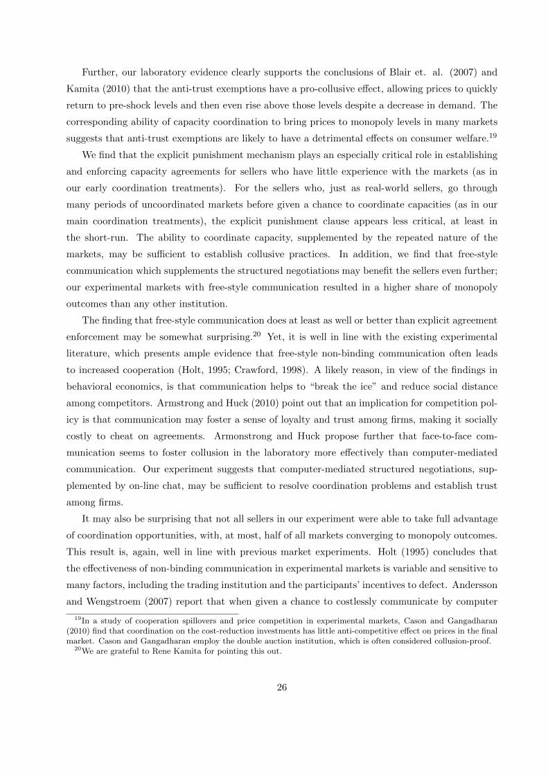
Further, our laboratory evidence clearly supports the conclusions of Blair et. al. (2007) and

Kamita (2010) that the anti-trust exemptions have a pro-collusive effect, allowing prices to quickly

return to pre-shock levels and then even rise above those levels despite a decrease in demand. The

corresponding ability of capacity coordination to bring prices to monopoly levels in many markets

suggests that anti-trust exemptions are likely to have a detrimental effects on consumer welfare.19

We find that the explicit punishment mechanism plays an especially critical role in establishing

and enforcing capacity agreements for sellers who have little experience with the markets (as in

our early coordination treatments). For the sellers who, just as real-world sellers, go through

many periods of uncoordinated markets before given a chance to coordinate capacities (as in our

main coordination treatments), the explicit punishment clause appears less critical, at least in

the short-run. The ability to coordinate capacity, supplemented by the repeated nature of the

markets, may be sufficient to establish collusive practices. In addition, we find that free-style

communication which supplements the structured negotiations may benefit the sellers even further;

our experimental markets with free-style communication resulted in a higher share of monopoly

outcomes than any other institution.

The finding that free-style communication does at least as well or better than explicit agreement

enforcement may be somewhat surprising.20 Yet, it is well in line with the existing experimental

literature, which presents ample evidence that free-style non-binding communication often leads

to increased cooperation (Holt, 1995; Crawford, 1998). A likely reason, in view of the findings in

behavioral economics, is that communication helps to “break the ice” and reduce social distance

among competitors. Armstrong and Huck (2010) point out that an implication for competition pol-

icy is that communication may foster a sense of loyalty and trust among firms, making it socially

costly to cheat on agreements. Armonstrong and Huck propose further that face-to-face com-

munication seems to foster collusion in the laboratory more effectively than computer-mediated

communication. Our experiment suggests that computer-mediated structured negotiations, sup-

plemented by on-line chat, may be sufficient to resolve coordination problems and establish trust

among firms.

It may also be surprising that not all sellers in our experiment were able to take full advantage

of coordination opportunities, with, at most, half of all markets converging to monopoly outcomes.

This result is, again, well in line with previous market experiments. Holt (1995) concludes that

the effectiveness of non-binding communication in experimental markets is variable and sensitive to

many factors, including the trading institution and the participants’ incentives to defect. Andersson

and Wengstroem (2007) report that when given a chance to costlessly communicate by computer

19In a study of cooperation spillovers and price competition in experimental markets, Cason and Gangadharan(2010) find that coordination on the cost-reduction investments has little anti-competitive effect on prices in the finalmarket. Cason and Gangadharan employ the double auction institution, which is often considered collusion-proof.

20We are grateful to Rene Kamita for pointing this out.

26

in a repeated Bertrand duopoly, subjects exchanged messages frequently, but they had difficulties

in maintaining collusive agreements. The two-stage Kreps and Sheinkman (1993) duopoly that we

study is arguably more complicated than Bertrand price-setting duopoly; we therefore consider the

observed 50% perfect collusion rate quite high.

It is notable that we obtain convincing evidence on the effects of capacity coordination on

industry outcomes despite the rather complex nature of the institution and the lack of experience

of our experimental subjects. One would expect the effects of capacity coordination to be even more

pronounced with experienced and highly motivated sellers. For this reason, we believe that these

experimental results, along with already existing empirical evidence, may have strong implications

for real-world industry practices.

Our findings suggest that capacity coordination may not be necessary to reduce capacities even

in industries in crises. Such conclusions should be drawn with some cautions though, as they may

be sensitive to the severity of the demand shock. In addition, cost structures in real-world industries

with advanced capacity settings may be more complex than in our experiment and involve high fixed

costs (other than capacity costs). Such high fixed costs may create extra difficulties for the firms

in industries in crises; capacity coordination may then help such firms to sustain a certain level of

profitability and avoid bankruptcies. What our experiments show is that persistent losses and firm

bankruptcies are unlikely to be solely due to excess capacities, as firms are able to quickly reduce

capacities even in the markets with no capacity coordination. Further, a common justification of

antitrust immunity is that capacity coordination is imperfect and consumers are still better off than

under monopoly. Our results demonstrate that some duopolists are able to reduce their capacities

to monopoly levels and set monopoly prices given an opportunity to coordinate capacities. Thus

capacity coordination by duopolists could potentially harm consumers as much as one firm going

bankrupt, and the other firm becoming the monopolist. And beyond doubt, we find that allowing

coordination harms consumers conditional on both firms surviving in the market.

References

[1] Albaek, S., Mollgaard, P., and Overgaard, P. “Government-Assisted Oligopoly Coordination?

A Concrete Case.” Journal of Industrial Economics, Vol. 45 (1997), pp. 429-443.

[2] Aloha Airlines, Inc. and Hawaiian Airline, Inc. “Joint Application of Aloha Airlines, Inc. and

Hawaiian Airlines, Inc. for Antitrust Immunity, Before the Department of Transportation.”

Docket OST-2002-13002-1, 2002.

[3] Andersson, O., and Wengstroem, E. “Do Antitrust Laws Facilitate Collusion? Experimental

Evidence on Costly Communication in Duopolies.” Scandinavian Journal of Economics, Vol.

109 (2007), pp. 331-339.

27

[4] Apesteguia, J., Dufwenberg, M., and Selten, R. “Blowing the whistle.” Economic Theory, Vol.

31 (2007), pp. 143-166.

[5] Armstrong, M., and Huck, S. “Behavioral Economics as Applied to Firms: A Primer.” Com-

petition Policy International, Vol. 6 (2010), pp. 3-45.

[6] Blair, R., Mak, J., and Bonham, C. “Collusive Duopoly: The Effects of the Aloha and Hawaiian

Airlines’ Agreement to Reduce Capacity.” Antitrust Law Journal, Vol. 74 (2007), pp. 409-438.

[7] Brown, A., Plott, C. and Sullivan, H. “The Nature of Collusion Facilitating and Collusion

Breaking Power of Simultaneous Ascending Price and Descending Price Auctions.” Economic

Inquiry, Vol. 47 (2009), pp. 395-424.

[8] Cason, T., Gangadharan, L. “Cooperation Spillovers and Price Competition in Experimental

Markets.” Mimeo, Purdue University, 2010.

[9] Crawford, V. “A Survey of Experiments on Communication via Cheap Talk.” Journal of

Economic Theory, Vol. 78 (1998), pp. 286-298.

[10] Davidson, C., Deneckere, R. “Long-Run Competition in Capacity, Short-Run Competition in

Price, and the Cournot Model.” Rand Journal of Economics, Vol. 17 (1986), pp. 404-415.

[11] Davis, D. “Advance Production and Cournot Outcomes: An Experimental Investigation.”

Journal of Economic Behavior and Organization, Vol. 40 (1999), pp. 59-79.

[12] Davis, D., Harrison, G., and Williams, A. “Convergence to Nonstationary Competitive Equi-

libria: An Experimental Analysis.” Journal of Economic Behavior and Organization, Vol. 22

(1993), pp. 305-326.

[13] Deck C., and B. Wilson. “Experimental Gasoline Markets.” Journal of Economic Behavior

and Organization, Vol. 67 (2008), pp. 134-149.

[14] Dufwenberg, M. and Gneezy, U. “Price Competition and Market Concentration: An Experi-

mental Study.” International Journal of Industrial Organization, Vol. 18 (2000), pp. 7-22.

[15] Durham, Y., McCabe, K., Olson, M., Rassenti, S., and Smith, V. “Oligopoly Competition in

Fixed Cost Environments.” International Journal of Industrial Organization, Vol. 22 (2004),

pp. 147-162.

[16] Eads, G. “Airline Capacity Limitations Controls: Public Vice or Public Virtue?” American

Economic Review, Papers and Proceedings, Vol. 64 (1974), pp. 365-371.

28

[17] Fischbacher, U. “z-Tree: Zurich Toolbox for Ready-made Economic Experiments.” Experimen-

tal Economics, Vol. 10 (2007), pp. 171-178.

[18] Fiebig, A. “Crisis Cartels and the Triumph of Industrial Policy over Competition Law in

Europe.” Brooklyn Journal of International Law, Vol. 25 (1999), pp. 607-638.

[19] Fouraker, L. and Siegel, S. Bargaining Behavior. McGraw-Hill, 1963.

[20] Grether D., and Plott, C. “The Effects of Market Practices in Oligopolistic Markets: an

Experimental Examination of the Ethyl Case.” Economic Inquiry, Vol. 22 (1984), pp. 470-507.

[21] Goodwin, D., and Mestelman, S. “A Note Comparing the Capacity Setting Performance of the

Kreps-Scheinkman Duopoly Model with the Cournot Duopoly Model in a Laboratory Setting.”

International Journal of Industrial Organization, Vol. 28 (2010), pp. 522-525.

[22] Hinloopen, J., and Soetevent, A. “Laboratory evidence on the effectiveness of corporate le-

niency programs.” RAND Journal of Economics, Vol. 39 (2008), pp. 607-616.

[23] Holt, C. “Industrial Organization: A Survey of Laboratory Research.” In J. Kagel and A.

Roth, eds., The Handbook of Experimental Economics. Princeton University Press, 1995.

[24] Huck, S., Normann, H., and Oechssler, J. “Two Are Few and Four Are Many: Number Effects

in Experimental Oligopolies.” Journal of Economic Behavior and Organization, Vol. 53 (2004),

pp. 435-446.

[25] Kamita, R. “Analyzing the Effects of Temporary Antitrust Immunity: The Aloha-Hawaiian

Immunity Agreement.” Journal of Law and Economics, Vol. 53 (2010), pp. 239-261.

[26] Kreps, D., and Sheinkman, J. “Quantity Precommitment and Bertrand Competition Yield

Cournot Outcomes.” Bell Journal of Economics, Vol. 14 (1983), pp. 326-337.

[27] Kruse, J., Rassenti, S., Reynolds, S., and Smith, V. “Bertrand-Edgeworth Competition in

Experimental Markets.” Econometrica, Vol. 62 (1994), pp. 343-371.

[28] Levenstein, M. and Suslow, V. “What Determines Cartel Success?” Journal of Economic

Literature, Vol. 44 (2006), pp. 43-95.

[29] Moreno, D. and Ubeda, L. “Capacity Precommitment and Price Competition Yield the

Cournot Outcome. Games and Economic Behavior, Vol. 56 (2006), pp. 323-332.

[30] Muren, A. “Quantity Precommitment In An Experimental Oligopoly Market.” Journal of

Economic Behavior and Organization, Vol. 41 (2000), pp. 147-157.

29

[31] Noussair, C., Plott, C., and Riezman, R. “An Experimental Investigation of the Patterns of

International Trade.” The American Economic Review, Vol. 85 (1995), pp. 462-491.

[32] Offerman, T., and Potters, J. “Does Auctioning of Entry Licences Induce Collusion? An

Experimental Study.” Review of Economic Studies, Vol. 73 (2006), pp. 769-791.

[33] Osborne, M., and Pitchik, C. “Price Competition in a Capacity-Constrained Duopoly.” Journal

of Economic Theory, Vol. 38 (1986), pp. 238-260.

[34] Peck, M., Levin, R., and Goto, A. “Picking Losers: Public Policy toward Declining Industries

in Japan.” Journal of Japanese Studies, Vol. 13 (1987), pp. 79-123.

[35] Plott, C. “An Updated Review of Industrial Organization Applications of Experimental Meth-

ods.” In R. Schmalensee and R. Willig, eds., The Handbook of Industrial Organization. New

York: North-Holland. Vol. 2. 1989.

[36] Rees, R. “Collusive Equilibrium in the Great Salt Duopoly.” The Economic Journal, Vol. 103

(1993), pp. 833-848.

[37] Simpson, P. “Response to Decline in the Western European Synthetic Fibre Industry: An

Investigation of a Crisis Cartel.” In P. Grossman, ed., How Cartels Endure and How they Fail.

Edward Elgar, 2004.

[38] Sjostrom, W. “Collusion in Ocean Shipping: A Test of Monopoly and Empty Core Models.”

The Journal of Political Economy, Vol. 97 (1989), pp. 1160-1179.

[39] Staiger R., and Wolak, F. “Collusive Pricing with Capacity Constraints in the Presence of

Demand Uncertainty.” The Rand Journal of Economics, Vol. 23 (1992), pp. 203-220.

[40] Tirole, J. Theory of Industrial Organization. MIT University Press, 1988.

[41] Van Boening, M., and Wilcox, N. “Avoidable Cost: Ride a Double Auction Roller Coaster.”

The American Economic Review, Vol. 86 (1996), pp. 461-477.

[42] Williams, A., and Smith, V. “Cyclical Double-Auction Markets With and Without Specula-

tors.” Journal of Business, Vol. 57 (1984), pp. 1-33.

30

TABLE 1. Summary of Experimental Sessions

Treatment Session ID Session Date LocationNo. of

MarketsNo. Paid Periods** Quiz?

1 5/4/2007 UHM 2 35 N4 5/22/2007 UHM 4 40 Y12 6/10/2010 UAA 4 39 Y2 5/10/2007 UHM 2 39 N3 5/18/2007 UHM 3 39 N5 5/23/2007 UHM 3 39 Y10 6/3/2010 UAA 3* 39 Y6 5/24/2007 UHM 4 39 Y9 4/27/2010 UAA 2 39 Y11 6/9/2010 UAA 4 39 Y7 9/28/2007 UHM 5 36 Y8 10/3/2007 UHM 2 39 Y13 6/17/2010 UAA 3 39 Y

No. of markets, main treatments 41

15 4/21/2011 UAA 3 31 Y17 4/27/2011 UAA 4 39 Y18 4/28/2011am UHM 4 24 Y14 4/15/2011 UAA 3* 39 Y16 4/26/2011 UHM 2 39 Y19 4/28/2011pm UHM 4 31 Y20 5/12/2011 UAA 4 39 Y

No. of markets, additional treatments 23Total No. of markets 64

Main treatments: No Negotiations and After-shock Negotiations

Additional treatments: Pre-shock Negotiations

*Sessions 10 and 14 originally had four independent markets each, but one market in each session was excluded due to bankruptcies**In treatments with negotiations, one unpaid instructional/trail period (period 25 in after-shock negotiations treatments and period 7 in pre-shock negotiations treatments) preceeded negotiations periods

Pre-shock Negotiations with Punishment

(PreshockNegPun)

Negotiation w/o Punishment (NegNoPun)

No Negotiation No Punishment

(NoNegNoPun)

Negotiation with Punishment (NegPun)

Negotiation w/o Punishment, with Chat

(NegChat)

Pre-shock Negotiations w/o Punishment

(PreshockNegNoPun)

TABLE 2. Average Total Market Capacity Before and After the Shock, physical units

VERY EARLY:

Per 1-7

EARLY BEFORE: Per. 8-14

BEFORE SHOCK:

Per. 15-21

SHOCK: Per. 22-24

EARLY AFTER:

Per. 25-31

LATE AFTER:

Per. 32-end

132 132 132 108 108 108176 176 176 144 144 144264 264 264 216 216 216

Mean 238.87 227.74 234.56 205.50 184.20 169.90(56.29) (52.31) (49.63) (58.50) (42.24) (34.70)

Mean 211.60 221.35 227.61 198.58 143.78 145.65(50.28) 53.78 81.99 52.15 33.59 33.92

Mean 278.21 277.71 234.24 211.87 146.64 161.19(119.56) (74.27) (52.83) (54.04) (38.86) (68.35)

Mean 250.79 254.49 230.36 212.13 178.61 144.92(76.52) (77.48) (51.52) (42.82) (65.64) (54.40)

Mean 266.12 204.21 187.26 162.58 128.39 127.03(93.07) (81.01) (37.18) (41.57) (23.32) (41.73)

Mean 277.17 226.43 254.02 211.06 199.96 183.67(61.24) (65.62) (51.92) (51.63) (69.98) (59.12)

MonopolyCournotBertrand

Benchmark Predictions:

PreShockNegPun (11 obs*)Standard Deviation

Standard Deviation

NegPun (11 obs)

Main treatments: No Negotiations and After-shock Negotiations

Additional treatments: Pre-shock Negotiations

*As some sessions in this treatment did not complete all periods because of time constraints, there are only 7 observations for Periods 25-31, and 4 observations for Periods 32-end **As some sessions in this treatment did not complete all periods because of time constraints, there are only 8 observations for Periods 32-end

NegChat (10 obs)

NoNegNoPun (10 obs)

Standard Deviation

Standard DeviationNegNoPun (10 obs)

Standard Deviation

PreShockNegNoPun (12 obs**)Standard Deviation

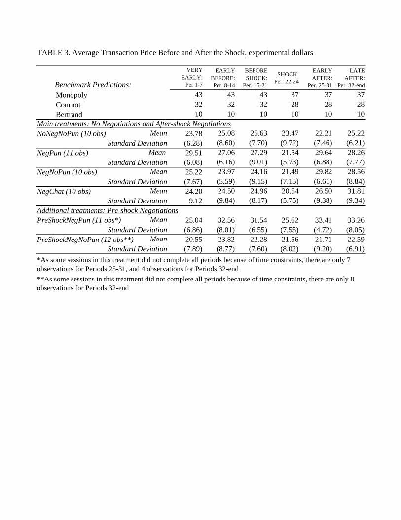
TABLE 3. Average Transaction Price Before and After the Shock, experimental dollars

VERY EARLY:

Per 1-7

EARLY BEFORE: Per. 8-14

BEFORE SHOCK:

Per. 15-21

SHOCK: Per. 22-24

EARLY AFTER:

Per. 25-31

LATE AFTER:

Per. 32-end

43 43 43 37 37 3732 32 32 28 28 2810 10 10 10 10 10

Mean 23.78 25.08 25.63 23.47 22.21 25.22(6.28) (8.60) (7.70) (9.72) (7.46) (6.21)

Mean 29.51 27.06 27.29 21.54 29.64 28.26(6.08) (6.16) (9.01) (5.73) (6.88) (7.77)

Mean 25.22 23.97 24.16 21.49 29.82 28.56(7.67) (5.59) (9.15) (7.15) (6.61) (8.84)

Mean 24.20 24.50 24.96 20.54 26.50 31.819.12 (9.84) (8.17) (5.75) (9.38) (9.34)

Mean 25.04 32.56 31.54 25.62 33.41 33.26(6.86) (8.01) (6.55) (7.55) (4.72) (8.05)

Mean 20.55 23.82 22.28 21.56 21.71 22.59(7.89) (8.77) (7.60) (8.02) (9.20) (6.91)

PreShockNegPun (11 obs*)

CournotBertrand

Standard Deviation

NegPun (11 obs)Standard Deviation

NegNoPun (10 obs)Standard Deviation

Main treatments: No Negotiations and After-shock Negotiations

Additional treatments: Pre-shock Negotiations

Standard DeviationPreShockNegNoPun (12 obs**)

Standard Deviation*As some sessions in this treatment did not complete all periods because of time constraints, there are only 7 observations for Periods 25-31, and 4 observations for Periods 32-end **As some sessions in this treatment did not complete all periods because of time constraints, there are only 8 observations for Periods 32-end

Benchmark Predictions:

NegChat (10 obs)

NoNegNoPun (10 obs)Standard Deviation

Monopoly

TABLE 4. Subject Per Period Profits Before and After the Shock, experimental dollars

VERY EARLY:

Per 1-7

EARLY BEFORE: Per. 8-14

BEFORE SHOCK:

Per. 15-21

SHOCK: Per. 22-24

EARLY AFTER:

Per. 25-31

LATE AFTER:

Per. 32-end

2178 2178 2178 1458 1458 14581936 1936 1936 1296 1296 1296

0 0 0 0 0 0

Mean 850.89 1133.87 1142.97 568.83 675.02 930.94(543.52) (603.50) (628.93) (516.68) (512.69) (426.23)

Mean 1188.26 1260.54 1261.85 648.06 1118.41 1122.80(406.08) (579.74) (830.16) (483.82) (346.21) (363.97)

Mean 686.98 781.16 1049.98 440.40 1021.18 855.34(1093.82) (701.91) (555.12) (525.43) (311.82) (509.69)

Mean 819.24 897.57 1091.24 502.57 716.70 1066.46(822.48) (844.78) (580.23) (342.83) (631.38) (439.37)

Mean 783.65 1383.96 1601.04 818.88 1181.81 1263.39(664.80) (635.26) (437.96) (500.35) (224.34) (237.70)

Mean 506.59 821.71 823.89 452.67 533.93 682.01(657.71) (531.58) (581.89) (477.27) (585.11) (474.41)

Bertrand

Benchmark Predictions:MonopolyCournot

NegChat (10 obs)Standard Deviation

NoNegNoPun (10 obs)Standard Deviation

NegPun (11 obs)Standard Deviation

Main treatments: No Negotiations and After-shock Negotiations

Additional treatments: Pre-shock Negotiations

*As some sessions in this treatment did not complete all periods because of time constraints, there are only 7 observations for Periods 25-31, and 4 observations for Periods 32-end **As some sessions in this treatment did not complete all periods because of time constraints, there are only 8 observations for Periods 32-end

NegNoPun (10 obs)Standard Deviation

PreShockNegPun (11 obs*)Standard Deviation

PreShockNegNoPun (12 obs**)Standard Deviation

TABLE 5: Summary of Capacity Negotiations in Markets with Free-Style Chat

Session location

Market ID

Range of Neg/chat periods

No. of Chat periods

No. of periods chat used

First period chat used

Last period chat used

Capacity discussed?

Agreed-upon capacity mean (stddv)

Actual p/p capacity mean (stddv)

UHM 701 25-38 12 12 25 38 yes 101.25 85.21(22.48) (29.48)

UHM 702 25-38 12 12 25 38 yes 112.27 101.25(15.71) (21.33)

UHM 703 25-38 12 5 26 35 yes 63.75 60.04(11.51) (4.92)

UHM 704 25-38 12 0 n/a n/a n/a 158.00 137.63 Chat was not used, capacity set too high(58.08) (24.90)

UHM 705 25-38 12 12 25 38 no 50.60 55.71(34.57) (45.22)

UHM 801 25-39 15 6 26 37 yes 60.00 57.27(0.00) (8.62)

UHM 802 25-39 15 0 n/a n/a n/a 57.33 69.97(15.45) (9.38)

UAA 1301 25-39 15 2 26 34 yes 130.50 114.27(68.72) (30.13)

UAA 1302 25-39 15 2 25 30 yes 53.33 52.10(10.47) (10.60)

UAA 1303 25-39 15 4 25 34 yes 84.00 81.13(55.27) (55.49)

*In market 701, specific capacity was not agreed upon in 4 negotiations periods

No chat, noisy capacity negotiations with frequent deviationsOnly used chat in 2 periods. Capacity set was highly variable and too highNegotiated effectively without chat. Used chat to restate capacity proposals in two periods only. Did not use chat much. Agreed on capacity of 50 only in period 34.

Summary of Chat content

Tried to implement a rotation shceme that only worked in the last 2 periodsChose too high a capacity of 120 per person, only lowered capacity in the last 2 periodsFirst time chat was used (period 26), agreed on a low capacity of 60

Did not discuss capacity or price, but still set low capacity Agreed on capacity of 60 in period 27; later used chat to confirm that this level worked well

No of obs

To Mono- poly

To Cournot

To Bert-rand

Cournot Best Res- ponse

TFT other's capa- city

TFT agree-ment

Agree-ment

compli-ance

Before 272 0.463 0.426 0.441 0.346 0.507 n/a n/aShock 60 0.433 0.383 0.350 0.350 0.500 n/a n/aAfter 300 0.410 0.383 0.317 0.350 0.510 n/a n/a

Before 308 0.416 0.484 0.448 0.383 0.510 n/a n/aShock 66 0.470 0.485 0.379 0.455 0.500 n/a n/aAfter 330 0.452 0.385 0.348 0.291 0.479 0.818 0.879

Before 280 0.425 0.439 0.486 0.364 0.432 n/a n/aShock 60 0.517 0.533 0.467 0.533 0.450 n/a n/aAfter 300 0.513 0.490 0.470 0.387 0.487 0.630 0.620

Before 280 0.486 0.496 0.525 0.386 0.486 n/a n/aShock 60 0.450 0.383 0.283 0.417 0.333 n/a n/aAfter 270 0.437 0.419 0.396 0.330 0.519 0.837 0.852

Before 308 0.549 0.571 0.490 0.477 0.474 0.860 0.922Shock 66 0.576 0.500 0.318 0.515 0.364 0.924 0.955After 184 0.467 0.326 0.332 0.326 0.560 0.918 0.962

Before 332 0.440 0.482 0.554 0.401 0.419 0.690 0.648Shock 72 0.639 0.597 0.472 0.556 0.556 0.736 0.639After 312 0.452 0.417 0.462 0.378 0.423 0.721 0.715

*From Period 8 onwards.

TABLE 6. Share of individual capacity choices consistent with behvaioral rules before, during and after the shock, by treatment*

PreShockNegNoPun

Benchmark Predictions:NoNegNoPun

NegPun

NegNoPun

NegChat

PreShockNegPun

Figure 1: Median market characteristics by period: No Negotiations compared to after‐shock Negotiation treatments pooled

100

120

140

160

180

200

220

240

260

280

1 2 3 4 5 6 7 8 9 10 11 12 13 14 15 16 17 18 19 20 21 22 23 24 25 26 27 28 29 30 31 32 33 34 35 36 37 38 39 40

Units

Median Capacity by Period

NoNegNoPun

NegPooled

Monopoly

Cournot

Bertrand

260

280Median Sales by Period

NoNegNoPun

5

10

15

20

25

30

35

40

45

1 2 3 4 5 6 7 8 9 10 11 12 13 14 15 16 17 18 19 20 21 22 23 24 25 26 27 28 29 30 31 32 33 34 35 36 37 38 39 40

Expe

rimen

tal D

ollars

Median Price by Period

NoNegNoPun

NegPooled

Monopoly

Cournot

Bertrand

PreShockNegNoPun

100

120

140

160

180

200

220

240

260

1 2 3 4 5 6 7 8 9 10 11 12 13 14 15 16 17 18 19 20 21 22 23 24 25 26 27 28 29 30 31 32 33 34 35 36 37 38 39 40

Units

NoNegNoPun

NegPooled

Monopoly

Cournot

Bertrand

0

500

1000

1500

2000

2500

1 2 3 4 5 6 7 8 9 10 11 12 13 14 15 16 17 18 19 20 21 22 23 24 25 26 27 28 29 30 31 32 33 34 35 36 37 38 39 40

Expe

rimen

tal D

ollars

Median Profit by Period

NoNegNoPun

NegPooled

Monopoly

Cournot

Bertrand

Figure 2: Median market characteristics by period, by treatment

100

120

140

160

180

200

220

240

260

280

300

1 2 3 4 5 6 7 8 9 10 11 12 13 14 15 16 17 18 19 20 21 22 23 24 26 27 28 29 30 31 32 33 34 35 36 37 38 39 40

Units

Median Capacity by Period

NoNegNoPun

NegNoPun

NegPun

NegChat

Monopoly

Cournot

Bertrand

260

280Median Sales by Period

NoNegNoPun

5

10

15

20

25

30

35

40

45

1 2 3 4 5 6 7 8 9 10 11 12 13 14 15 16 17 18 19 20 21 22 23 24 26 27 28 29 30 31 32 33 34 35 36 37 38 39 40

Expe

rimen

tal D

ollars

Median Price by Period

NoNegNoPun

NegNoPun

NegPun

NegChat

Monopoly

Cournot

Bertrand

100

120

140

160

180

200

220

240

260

280

1 2 3 4 5 6 7 8 9 10 11 12 13 14 15 16 17 18 19 20 21 22 23 24 26 27 28 29 30 31 32 33 34 35 36 37 38 39 40

Units

NoNegNoPun

NegNoPun

NegPun

NegChat

Monopoly

Cournot

Bertrand

0

500

1000

1500

2000

2500

1 2 3 4 5 6 7 8 9 10 11 12 13 14 15 16 17 18 19 20 21 22 23 24 26 27 28 29 30 31 32 33 34 35 36 37 38 39 40

Expe

rimen

tal D

ollars

Median Profit by Period

NoNegNoPun

NegNoPun

NegPun

NegChat

Monopoly

Cournot

Bertrand

Figure 3: Median market characteristics in early negotiations treatments, by period

100

120

140

160

180

200

220

240

260

280

300

1 2 3 4 5 6 7 8 9 10 11 12 13 14 15 16 17 18 19 20 21 22 23 24 25 26 27 28 29 30 31 32 33 34 35 36 37 38 39 40

Units

Median Capacity by Period

PreShockNegPun

PreShockNegNoPun

Monopoly

Cournot

Bertrand

260

280Median Sales by Period

PreShockNegPun

5

10

15

20

25

30

35

40

45

1 2 3 4 5 6 7 8 9 10 11 12 13 14 15 16 17 18 19 20 21 22 23 24 25 26 27 28 29 30 31 32 33 34 35 36 37 38 39 40

Expe

rimen

tal D

ollars

Median Price by Period

PreShockNegPun

PreShockNegNoPun

Monopoly

Cournot

Bertrand

PreShockNegNoPun

100

120

140

160

180

200

220

240

260

1 2 3 4 5 6 7 8 9 10 11 12 13 14 15 16 17 18 19 20 21 22 23 24 25 26 27 28 29 30 31 32 33 34 35 36 37 38 39 40

Units

PreShockNegPun

PreShockNegNoPun

Monopoly

Cournot

Bertrand

0

500

1000

1500

2000

2500

1 2 3 4 5 6 7 8 9 10 11 12 13 14 15 16 17 18 19 20 21 22 23 24 25 26 27 28 29 30 31 32 33 34 35 36 37 38 39 40

Expe

rimen

tal D

ollars

Median Profit by Period

PreShockNegPun

PreShockNegNoPun

Monopoly

Cournot

Bertrand

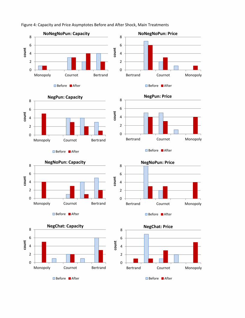
Figure 4: Capacity and Price Asymptotes Before and After Shock, Main Treatments

0

2

4

6

8

Monopoly Cournot Bertrand

coun

t

NoNegNoPun: Capacity 

Before After

0

2

4

6

8

Monopoly Cournot Bertrand

coun

t

NegPun: Capacity 

Before After

6

8NegNoPun: Capacity  

0

2

4

6

8

Bertrand Cournot Monopoly

coun

t

NoNegNoPun: Price 

Before After

0

2

4

6

8

Bertrand Cournot Monopoly

coun

t

NegPun: Price 

Before After

6

8NegNoPun: Price 

0

2

4

6

8

Monopoly Cournot Bertrand

coun

t

NegNoPun: Capacity  

Before After

0

2

4

6

8

Monopoly Cournot Bertrand

coun

t

NegChat: Capacity 

Before After

0

2

4

6

8

Bertrand Cournot Monopoly

coun

t

NegNoPun: Price 

Before After

0

2

4

6

8

Bertrand Cournot Monopoly

coun

t

NegChat: Price 

Before After

Figure 5: Capacity and Price Asymptotes Before and After Shock, Pre‐Shock Negotiations Treatments

0

2

4

6

8

Monopoly Cournot Bertrand

coun

t

PreShockNegPun: Capacity  

Before After

‐1

1

3

5

7

9

Monopoly Cournot Bertrand

coun

t

PreShockNegNoPun: Capacity 

Before After

0

2

4

6

8

Bertrand Cournot Monopoly

coun

t

PreShockNegPun: Price 

Before After

‐1

1

3

5

7

9

Bertrand Cournot Monopoly

coun

t

PreShockNegNoPun: Price 

Before After

Appendix A

Experiment Instructions1 Introduction You are about to participate in an experiment in the economics of market decision making in which you will earn money based on the decisions you make. All earnings you make are yours to keep and will be paid to you IN CASH at the end of the experiment. During the experiment all units of account will be in experimental dollars. Upon concluding the experiment, you will paid 1 dollar in cash for every 1750 experimental dollars you earn in the experiment. Your cash earnings plus a show up payment of 5 dollars will be paid to you in private. You will begin the experiment with 7500 experimental dollars. This is NOT part of your show-up payment. Note your Current Earnings in the box at the top of the screen. Do not communicate with the other participants except according to the specific rules of the experiment. If you have a question, feel free to raise your hand. An experimenter will come over to you and answer your question in private. If you have any questions at this point, please raise your hand. Click Continue when you are ready go on.

_________________________________________________________ Markets and Trading Periods In this experiment you are going to participate in a market in which you will be selling units of a fictitious good. At the beginning of the experiment, you will be assigned to a market with another participant. You will not be told which of the other participants is in your market. What happens in your market has no effect on the participants in other markets and vice versa. You will remain in the same market with the same other seller until the end of the experimental session. This does not include trial periods. In trial periods, you may be matched with another individual. In this experiment, you will be referred to by your seller ID number. Your seller number will be assigned to you by the computer and displayed to you in the upper left hand corner.

1 Instructions were provided to the students in an interactive format via their computer terminals.

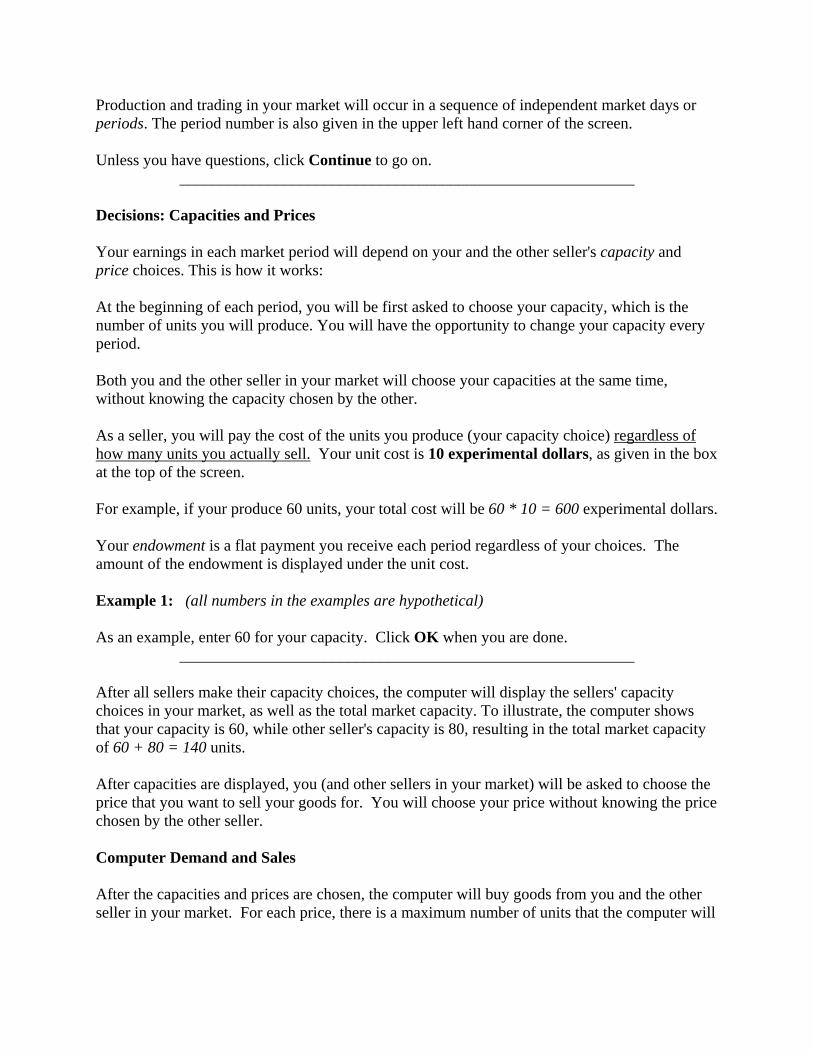
Production and trading in your market will occur in a sequence of independent market days or periods. The period number is also given in the upper left hand corner of the screen. Unless you have questions, click Continue to go on.

_________________________________________________________ Decisions: Capacities and Prices Your earnings in each market period will depend on your and the other seller's capacity and price choices. This is how it works: At the beginning of each period, you will be first asked to choose your capacity, which is the number of units you will produce. You will have the opportunity to change your capacity every period. Both you and the other seller in your market will choose your capacities at the same time, without knowing the capacity chosen by the other. As a seller, you will pay the cost of the units you produce (your capacity choice) regardless of how many units you actually sell. Your unit cost is 10 experimental dollars, as given in the box at the top of the screen. For example, if your produce 60 units, your total cost will be 60 * 10 = 600 experimental dollars. Your endowment is a flat payment you receive each period regardless of your choices. The amount of the endowment is displayed under the unit cost. Example 1: (all numbers in the examples are hypothetical) As an example, enter 60 for your capacity. Click OK when you are done.

_________________________________________________________ After all sellers make their capacity choices, the computer will display the sellers' capacity choices in your market, as well as the total market capacity. To illustrate, the computer shows that your capacity is 60, while other seller's capacity is 80, resulting in the total market capacity of 60 + 80 = 140 units. After capacities are displayed, you (and other sellers in your market) will be asked to choose the price that you want to sell your goods for. You will choose your price without knowing the price chosen by the other seller. Computer Demand and Sales After the capacities and prices are chosen, the computer will buy goods from you and the other seller in your market. For each price, there is a maximum number of units that the computer will

buy at this price, called Computer Demand. The lower the price, the higher the number of goods demanded. The exact number of units the computer will demand (buy) at any price is given by the following expression: Units Bought = 304 - ( 4 * Price ) You have a paper chart showing the computer demand at any price. This expression may change at any time. If it does, you will be informed. The computer will always buy first from the seller offering the lowest price. It will buy as many units as it demands at this price, or until it exhausts the low price seller's capacity. If the computer can still buy more units after buying all the units produced by the first seller, it will then buy from the seller with the higher price until it satisfies all the demand at the higher price, or until it exhausts all the capacity of the high price seller. To continue with our example, enter a price of 50 and click OK to continue.

_________________________________________________________ Suppose the other seller charged a price of 55. Because your price (50) is lower, the computer will buy your units first. At a price of 50, the computer will buy all 60 units that you've produced. The total number the computer would be willing to buy at this price would be 304 - (4 * 50) = 104 units. You can confirm this by looking at the demand chart provided to you. But since you've only produced 60, that is all that the computer purchases. After buying all of your units, the computer would then consider how many more units to purchase at the higher price of 55 being offered by the other seller. At this price, the computer demands 304 - (4 * 55) = 84 units. However, because the computer has already purchased 60 units from you, it will only purchase 84 - 60 = 24 units from the other seller. Your earnings are equal to the difference between your revenue from sales and the cost of all the units you have produced, plus your endowment. That is: YOUR EARNINGS = YOUR REVENUE - TOTAL COST + ENDOWMENT Your revenue is equal to the price you charge times the number of units you sell at this price: YOUR REVENUE = YOUR PRICE * QUANTITY SOLD Your total cost is equal to per unit cost of production times the number of unit that you produce (your capacity): YOUR TOTAL COST = PER UNIT COST * YOUR CAPACITY

In our example, if you produce 60 units at the unit cost of 10, and you sell all 60 units at the price of 50, then your revenue, cost and earnings are: YOUR REVENUE = (60 * 50) = 3000 YOUR TOTAL COST = 60 * 10 = 600 YOUR EARNINGS = 3000 - 600 + 50 = 2450 When you understand these results, click OK to continue.

_________________________________________________________ Example 2: (all numbers in the examples are hypothetical) Alternatively, imagine the following situation: Your Capacity: 200 Other's Capacity: 80 Your Price: 15 Other's Price: 15 If both sellers charge the same price, then the computer will buy an equal number of units from both buyers to the point where the computer's demand is satisfied. If the lower capacity seller sells every unit he or she produced and the computer still demands more, the computer will buy those units from the higher capacity seller until it has all the additional units it demands at the charged price or until they have purchased all of the additional units offered by the higher production seller. In the above example, the computer demand at the price of 15 is 304 - (4 * 15) = 244 units. Since both sellers are charging the same price, the computer will try to buy half of the demand, which is 244 / 2 = 122 units from each seller. However, because the other seller's capacity is set to only 80 units, the computer will buy all 80 units from this seller, and the remaining 244 - 80 = 164 units from you. Therefore, your earnings in this period will be: Earnings = (Price * Sales) + (Unit Cost * Capacity) + Endowment = (15 * 164) - (10 * 200) + 50 = 2460 - 2000 + 50 = 510 Click OK to continue.

_________________________________________________________ Example 3: (all numbers in the examples are hypothetical) Now suppose the capacity and price choices are as given below: \par \line \tab Your Capacity: 80

Other's Capacity: 100 Your Price: 50 Other's Price: 20 In this example, the other seller is the low-price seller, so the computer will buy from that seller first. The computer demand at the low price of 20 is 304 - (4 * 20) = 224 units, but since the other seller has only produced 100 units, the computer will buy all 100 units from this seller first. To check whether the computer will buy any from you, note that at the price of 50 that you've charged, the computer demand is 304 - (4 * 50) = 104 units. Since the computer has already bought 100 units from the other seller, it will buy 104 - 100 = 4 units from you. Therefore, your earnings in this period will be: Earnings = (Price * Sales) - (Unit Cost * Capacity) + Endowment = = (50 * 4) - (10 * 80) + 50 = 200 - 800 + 50 = -550 Please click OK to continue.

_________________________________________________________ Calculator In order to help you determine the potential profits in light of the decisions of you and the other seller, you have access to the Calculator at all times. This allows you to explore hypothetical situations before actually making your decisions. You may want to try it out now. Example #4: Your Capacity: 80 Other's Capacity: 50 Your Price: 8 Other's Price: 30 Example #5 Your Capacity: 120 Other's Capacity: 50 Your Price: 46 Other's Price: 38 This process will continue for a number of periods. A history window at the bottom of your screen will allow you to keep track of capacity choices, price choices, and the resulting profits from all of the previous periods. You may scroll up and down the history window.

The next period will be a trial period. It will not count towards your earnings. After you feel satisfied you understand the experiment, click Continue to finish the instructions.

_________________________________________________________ [The following instructions were presented to subjects in period 25 in the capacity negotiation treatments.] Capacity Coordination In this portion of the experiment, you and the other seller in your market will have the opportunity to coordinate your capacities prior to setting them. Each of you will have the ability to propose a CAPACITY FOR EACH SELLER in your market. For example, if you propose a capacity of 150, it means that the total proposed capacity in your market is 2 sellers * 150 units each = 300 units. You can change this proposal as many times as you like during this coordination stage. When you propose a capacity setting, the other seller sees your proposal and vice versa. During this stage, you can change your proposal as many times as you like. When you change your proposal, the other seller sees that change in real time. Try entering a number of capacity proposals now to see how it works. At any point during this stage, you or the other seller can end the stage by clicking Accept Proposal. This accepts the most recent capacity proposal of the other seller and becomes a capacity agreement between the two of you. Be careful when you choose to accept a proposal. It can be changed at any time up until the moment you click the button. If the time elapses in this stage without either seller clicking Accept Proposal, there is no capacity agreement for the period. Feel free to coordinate a capacity agreement now. The next stage starts after you or the other seller in your market accepts a proposal, or time elapses. Please note that your decisions in this period will not affect your earnings. This period is for instruction alone.

_________________________________________________________ Decisions After you agree on the capacity, the agreed capacity will be shown as in the box to the right. The experiment will then proceed as before. You will be asked to enter your capacity choice, and then your price. Note that in your capacity choice YOU ARE NOT CONSTRAINED TO ADHERE TO THE CAPACITY AGREEMENT. You may enter whatever capacity you wish. [The following text only appears in the instructions for the punishment treatments]

However, if you choose to exceed the agreed capacity, you will be liable to pay a penalty of 7 experimental dollars per unit of capacity you produce over the agreed amount. This penalty will be added to the earnings of the other seller in your market. Likewise, if the other seller exceeds the agreed capacity, they will pay a penalty to you. If both of you exceed the agreed capacity, the penalties will offset with the actual transfer of money depending on the relative sizes of the excess capacities. [end condition] Enter your capacity choice now.

_________________________________________________________ Then enter a price.

_________________________________________________________ The results screen will then indicate your price, sales and costs, as well as whether you have exceeded the agreed upon capacity, and will calculate your resulting earnings. [The following text only appears in the instructions for the punishment treatments] Note that, in addition to your normal earnings, you may also receive and/or pay a penalty based on your capacity decisions relative to the agreed capacity. If neither of you had exceeded the agreed capacity, neither of you would have to pay a penalty. Also note that your calculator will NOT include penalties in its calculation of profit. [end condition] Please note that, in future rounds, you will be matched with the same other seller as you were in previous rounds. These future rounds count toward your earnings. If you are ready to proceed, click OK.

_________________________________________________________

Quiz

EXERCISES

Use the calculator to answer the following questions. Suppose yours and the other seller’s capacity and price choices are as suggested in Example 4:

Your capacity: 80 Other’s Capacity: 50 Your price: 8 Other’s price: 30 1.1 Will the computer buy from you or the other seller first? (Check one)

_____ you; _____ other seller 1.2 What are your sales? ____ Do you sell all your capacity? ______ yes; _____ no 1.3 What are your earnings? ____ Do you earn or lose money? _____earn; ____ lose 1.4 Suppose the capacity choices and the other seller’s price stay unchanged. Suppose you could

change the price, calculate how your earnings for each of the following price choices:

Price:__ $5experimental; Your Earnings: __________ Price:__ 10 experimental; Your Earnings: __________ Price:__ 20 experimental; Your Earnings: __________ Price:__ 30 experimental; Your Earnings: __________ Price:__ 40 experimental; Your Earnings: __________ Price:__ 50 experimental; Your Earnings: __________ Price:__ 100 experimental; Your Earnings: _________

1.5 From Question 1.4 above, what would be the lowest price that would allow you not to lose

money? _____

1.6 From Question 1.4 above, at which price will you earn the most money?

The price is: _______ Your earnings will be equal to ___________ 1.7 Suppose now that you choose the price that allows you to earn most money, as in question

1.6 above. (Suppose, as before, that the capacity and price choices of the other sellers stay unchanged.) Given this price, how can you change your capacity to increase your earnings?

Price: _____ New capacity: _____ Your earnings: ___________ Are there any questions?

Appendix B: Subject decision screen: price-setting stage

Appendix C: Additional Tables

Table 7: Treatment effects: Cross-sectional time-series generalized least squares regressions

Coef. Std. Err. P>z Coef. Std. Err. P>z Coef. Std. Err. P>zConstant 246.57 (7.45) 0.000 23.71 (0.88) 0.000 877.79 (72.84) 0.000NegNoPun 6.36 (14.78) 0.667 3.00 (1.66) 0.071 59.61 (133.82) 0.656NegPun -51.41 (10.24) 0.000 7.70 (1.42) 0.000 465.05 (105.35) 0.000NegChat -8.43 (13.53) 0.533 2.11 (1.83) 0.248 35.55 (140.07) 0.800PreNegNoPun 27.43 (13.60) 0.044 -4.14 (1.72) 0.016 -336.92 (127.25) 0.008PreNegPun 5.75 (11.73) 0.624 2.68 (1.58) 0.090 7.73 (112.92) 0.945Periods8-21,NoNegNoPun -9.56 (7.83) 0.222 1.42 (0.93) 0.126 235.56 (82.67) 0.004Periods8‐21,NegNoPun 2.33 (13.86) 0.866 -3.31 (1.55) 0.033 42.81 (125.79) 0.734Periods8‐21,NegPun 1.69 (7.65) 0.825 -2.31 (1.18) 0.050 171.28 (85.87) 0.046Periods8‐21,NegChat -1.89 (10.67) 0.860 0.61 (1.53) 0.693 138.62 (117.28) 0.237Periods8-21,PreNegNoPun -38.32 (12.03) 0.001 2.59 (1.38) 0.060 190.02 (114.18) 0.096Periods8-21,PreNegPun -57.39 (9.86) 0.000 6.96 (1.41) 0.000 693.52 (96.54) 0.000Shock -32.57 (10.23) 0.001 -2.03 (1.22) 0.096 -285.25 (110.17) 0.010Shock, NegNoPun 17.48 (20.91) 0.403 -6.35 (2.38) 0.008 -362.38 (200.06) 0.070Shock, NegPun 23.78 (14.35) 0.098 -4.57 (1.97) 0.020 -225.32 (158.77) 0.156Shock, NegChat 12.51 (17.35) 0.471 -2.30 (2.35) 0.329 -392.21 (189.10) 0.038Shock,PreNegNoPun -26.33 (18.79) 0.161 0.57 (2.18) 0.794 49.67 (186.42) 0.790Shock,PreNegPun -49.58 (16.63) 0.003 2.60 (2.23) 0.244 286.55 (169.59) 0.091After shock -56.52 (10.02) 0.000 -0.43 (1.18) 0.715 -46.26 (99.94) 0.643After shock, NegNoPun -36.91 (20.17) 0.067 2.02 (2.28) 0.375 46.97 (184.56) 0.799After shock, NegPun 14.33 (13.87) 0.302 -0.90 (1.92) 0.639 -249.62 (145.19) 0.086After shock, NegChat 24.86 (17.79) 0.162 -1.21 (2.41) 0.617 -424.98 (187.16) 0.023After shock,PreNegNoPun -7.24 (18.48) 0.695 -0.75 (2.25) 0.738 -18.76 (174.53) 0.914After shock,PreNegPun -49.06 (16.86) 0.004 5.06 (2.22) 0.022 345.73 (160.71) 0.031Late after shock, NoNeg -14.54 (8.03) 0.070 1.42 (0.96) 0.138 164.19 (86.48) 0.058Late after shock,NegNoPun 14.01 (14.44) 0.332 -2.46 (1.63) 0.130 -168.15 (132.46) 0.204Late after shock,NegPun -2.98 (7.97) 0.708 -0.32 (1.22) 0.794 87.08 (90.66) 0.337Late after shock,NegChat -26.77 (10.98) 0.015 4.71 (1.58) 0.003 308.27 (121.20) 0.011Late after shock,PreNegNoPu -19.92 (15.04) 0.185 1.39 (1.67) 0.405 228.75 (137.13) 0.095Late after shock,PreNegPun -12.92 (12.99) 0.320 1.83 (1.78) 0.303 47.03 (129.69) 0.717

Number of obs 2357 2355* 2357

Log likelihood ‐12487 ‐7454 ‐17815

Heteroskedastic panels; panel-specific autocorrepaltion AR(1)*Trading price observations are missing for cases of zero sales (two cases)

Market Capacity Average trading price Average seller profit

TABLE 8 Capacity agreements in main negotiations treatments, physical units per seller

Agreed Capacity

Actual Capacity

Capacity Deviation

Agreed Capacity

Actual Capacity

Capacity Deviation

Agreed Capacity

Actual Capacity

Capacity Deviation

Mean 92.31 84.08 0.0527(20.72) (16.86)

Mean 78.67 71.61 -6.89 82.44 72.90 -9.54 0.9658 0.9658 0.8310(23.14) (16.32) (7.91) (28.21) (17.19) (22.71)

Mean 65.64 72.61 6.23 71.01 80.26 8.64 0.2322 0.4922 0.8458(15.83) (18.69) (17.95) (26.13) (33.11) (32.59)

Mean 98.84 90.69 -11.14 76.66 73.82 0.36 0.0098 0.0274 0.0040(43.25) (33.19) (12.18) (33.28) (29.41) (8.70)

p-value:* NegPun=NegNoPun 0.1053 0.9439 0.0112 0.2050 0.8880 0.0183p-value:* NegNoPun=NegChat 0.0288 0.2798 0.0052 0.6842 0.6842 0.0524p-value:* NegPun=NegChat 0.2908 0.2050 0.5261 0.3240 0.7782 0.3964* Wilcoxon Mann Whitney ranksum test** Wilcoxon signed rank test

NegNoPun (10 obs)Standard Deviation

NegChat (10 obs)Standard Deviation

Standard Deviation

p-value:** Early=LateEarly Negotiations:

Periods 25-31Late Negotiations:

Periods 32-end

NoNegNoPun (10 obs)Standard Deviation

NegPun (11 obs)

Treatment

TABLE 9: Capacity Asymptotes Before and After the Shock

market ID

capa-city asym-tote

Std. Err.

p-value: Cap=132 (Monop)

p-value: Cap=176 (Cournot)

p-value: Cap=264

(Bert-rand)

Classifi-cation

capa-city asym-tote

Std. Err.

p-value: Cap=108 (Monop)

p-value: Cap=144 (Cournot)

p-value: Cap=216

(Bert-rand)

Classifi-cation

p-value: before==after

Direc-tion of change

NoNegNoPun treatment101 240.58 10.93 0.0000 0.0000 0.0321 Bert/Cour 192.51 14.33 0.0000 0.0007 0.1011 Bertrand 0.0071 down102 237.13 9.35 0.0000 0.0000 0.0040 Bert/Cour 235.16 12.08 0.0000 0.0000 0.1128 Bertrand 0.8976 same401 194.18 15.46 0.0001 0.2398 0.0000 Cournot 149.14 18.30 0.0246 0.7789 0.0003 Cournot 0.0638 same402 250.85 6.81 0.0000 0.0000 0.0534 Bertrand 170.42 8.18 0.0000 0.0012 0.0000 Bert/Cour 0.0000 down403 138.97 3.85 0.0701 0.0000 0.0000 Monop 108.68 4.64 0.8831 0.0000 0.0000 Monop 0.0000 down404 277.09 15.48 0.0000 0.0000 0.3978 Bertrand 179.68 17.94 0.0001 0.0467 0.0429 Bert/Cour 0.0001 down1201 292.07 22.13 0.0000 0.0000 0.2046 Bertrand 142.83 27.35 0.2028 0.9660 0.0075 Cournot 0.0000 down1202 311.37 9.24 0.0000 0.0000 0.0000 above Bert 178.39 11.57 0.0000 0.0030 0.0012 Bert/Cour 0.0000 down1203 178.66 6.15 0.0000 0.6657 0.0000 Cournot 155.56 7.54 0.0000 0.1251 0.0000 Cournot 0.0196 down1204 186.56 7.63 0.0000 0.1666 0.0000 Cournot 165.66 9.51 0.0000 0.0227 0.0000 Bert/Cour 0.0890 sameNegNoPun treatment601 275.14 21.20 0.0000 0.0000 0.5995 Bertrand 116.69 25.65 0.7347 0.2871 0.0001 Monop 0.0000 down602 212.05 10.45 0.0000 0.0006 0.0000 Bert/Cour 161.95 13.02 0.1680 Cournot 0.0029 down603 195.51 7.93 0.0000 0.0139 0.0000 Bert/Cour 105.16 10.00 0.7766 0.0001 0.0000 Monop 0.0000 down604 297.98 32.05 0.0000 0.0001 0.2890 Bertrand 309.24 40.03 0.0000 0.0000 0.0199 above Bert 0.8272 same901 202.05 7.70 0.0000 0.0007 0.0000 Bert/Cour 107.00 9.68 0.9176 0.0001 0.0000 Monop 0.0000 down902 244.14 16.81 0.0000 0.0001 0.2375 Bertrand 241.57 21.18 0.0000 0.0000 0.2273 Bertrand 0.9240 same1101 330.54 27.24 0.0000 0.0000 0.0146 above Bert 166.87 33.61 0.0798 0.4962 0.1438 Cournot 0.0002 down1102 261.13 21.78 0.0000 0.0001 0.8952 Bertrand 138.64 27.49 0.2650 0.8456 0.0049 Cournot 0.0004 down1103 188.69 86.19 0.5107 0.8829 0.3822 Cournot 89.09 105.88 0.8582 0.6040 0.2307 Monop 0.4729 same1104 224.28 4.05 0.0000 0.0000 0.0000 Bert/Cour 181.22 5.09 0.0000 0.0000 0.0000 Bert/Cour 0.0000 down"Bert/Cour" ("Cour/Monop") indicates that the asymptote is between Bertrand and Cournot (Cournot and Monopoly) predictions.

Before Shock After Shock

TABLE 9 (continued): Capacity Asymptotes Before and After the Shock

market ID

capa-city asym-tote

Std. Err.

p-value: Cap=132 (Monop)

p-value: Cap=176 (Cournot)

p-value: Cap=264

(Bert-rand)

Classifi-cation

capa-city asym-tote

Std. Err.

p-value: Cap=108 (Monop)

p-value: Cap=144 (Cournot)

p-value: Cap=216

(Bert-rand)

Classifi-cation

p-value: before==after

Direc-tion of change

NegPun treatment201 365.45 13.90 0.0000 0.0000 0.0000 above Bert 101.85 17.34 0.7227 0.0151 0.0000 Monop 0.0000 down202 174.25 4.17 0.0000 0.6754 0.0000 Cournot 180.34 5.08 0.0000 0.0000 0.0000 Bert/Cour 0.3635 same301 284.63 11.34 0.0000 0.0000 0.0689 Bertrand 201.56 14.27 0.0000 0.0001 0.3115 Bertrand 0.0000 down302 205.55 14.68 0.0000 0.0441 0.0001 Bert/Cour 156.51 18.41 0.0084 0.4967 0.0012 Cournot 0.0377 down303 201.81 7.25 0.0000 0.0004 0.0000 Bert/Cour 196.08 9.15 0.0000 0.0000 0.0295 Bert/Cour 0.6215 same501 343.80 16.40 0.0000 0.0000 0.0000 above Bert 106.05 20.06 0.9225 0.0585 0.0000 Monop 0.0000 down502 178.91 9.39 0.0000 0.7564 0.0000 Cournot 149.09 11.82 0.0005 0.6670 0.0000 Cournot 0.0476 down503 188.43 6.09 0.0000 0.0414 0.0000 Bert/Cour 114.44 7.57 0.3952 0.0001 0.0000 Monop 0.0000 down1001 200.95 6.81 0.0000 0.0002 0.0000 Bert/Cour 159.09 8.58 0.0000 0.0788 0.0000 Cournot 0.0001 down1002 169.50 8.30 0.0000 0.4336 0.0000 Cournot 112.86 10.45 0.6417 0.0029 0.0000 Monop 0.0000 down1003 188.40 8.84 0.0000 0.1609 0.0000 Cournot 93.32 10.93 0.1792 0.0000 0.0000 Monop 0.0000 downNegChat treatment701 258.61 18.57 0.0000 0.0000 0.7717 Bertrand 157.57 26.81 0.0644 0.6126 0.0293 Cournot 0.0021 down702 325.95 16.78 0.0000 0.0000 0.0002 above Bert 194.36 24.48 0.0004 0.0396 0.3768 Bertrand 0.0000 down703 149.95 5.35 0.0008 0.0000 0.0000 Cour,Monop 114.03 7.23 0.4045 0.0000 0.0000 Monop 0.0001 down704 301.41 18.67 0.0000 0.0000 0.0451 above Bert 257.12 26.85 0.0000 0.0000 0.1256 Bertrand 0.1804 same705 308.09 25.93 0.0000 0.0000 0.089 Bertrand 84.91 36.94 0.5319 0.1097 0.0004 Monop 0.0000 down801 217.28 8.21 0.0000 0.0000 0.0000 Bert/Cour 116.35 10.32 0.4181 0.0074 0.0000 Monop 0.0000 down802 171.15 6.66 0.0000 0.466 0.0000 Cournot 137.48 8.03 0.0002 0.4174 0.0000 Cournot 0.0016 down1301 277.04 16.61 0.0000 0.0000 0.4325 Bertrand 221.24 20.99 0.0000 0.0002 0.8027 Bertrand 0.0356 down1302 175.44 14.27 0.0023 0.9688 0.0000 Cournot 87.59 17.76 0.2505 0.0015 0.0000 Monop 0.0001 down1303 301.56 39.54 0.0000 0.0015 0.3421 Bertrand 110.69 47.88 0.9552 0.4867 0.0279 Monop 0.0026 down"Bert/Cour" ("Cour/Monop") indicates that the asymptote is between Bertrand and Cournot (Cournot and Monopoly) predictions.

Before Shock After Shock

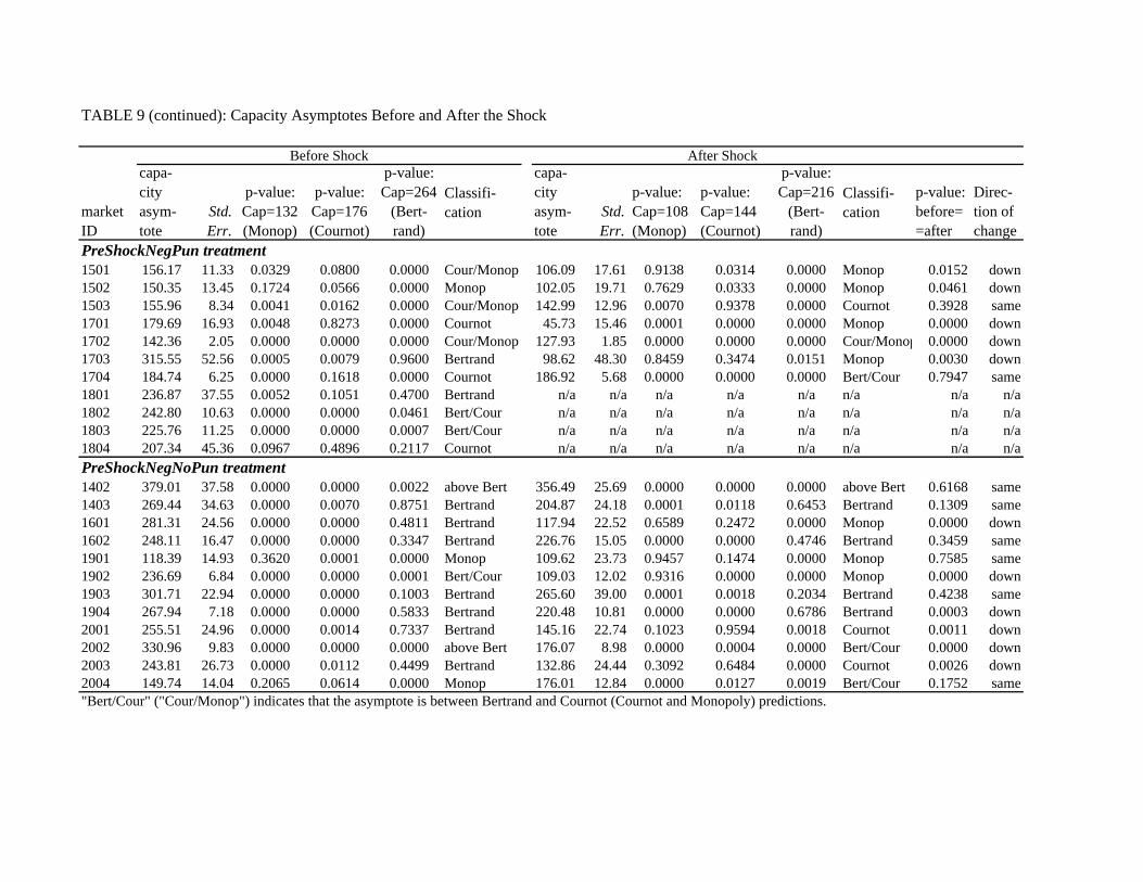
TABLE 9 (continued): Capacity Asymptotes Before and After the Shock

market ID

capa-city asym-tote

Std. Err.

p-value: Cap=132 (Monop)

p-value: Cap=176 (Cournot)

p-value: Cap=264

(Bert-rand)

Classifi-cation

capa-city asym-tote

Std. Err.

p-value: Cap=108 (Monop)

p-value: Cap=144 (Cournot)

p-value: Cap=216

(Bert-rand)

Classifi-cation

p-value: before==after

Direc-tion of change

PreShockNegPun treatment1501 156.17 11.33 0.0329 0.0800 0.0000 Cour/Monop 106.09 17.61 0.9138 0.0314 0.0000 Monop 0.0152 down1502 150.35 13.45 0.1724 0.0566 0.0000 Monop 102.05 19.71 0.7629 0.0333 0.0000 Monop 0.0461 down1503 155.96 8.34 0.0041 0.0162 0.0000 Cour/Monop 142.99 12.96 0.0070 0.9378 0.0000 Cournot 0.3928 same1701 179.69 16.93 0.0048 0.8273 0.0000 Cournot 45.73 15.46 0.0001 0.0000 0.0000 Monop 0.0000 down1702 142.36 2.05 0.0000 0.0000 0.0000 Cour/Monop 127.93 1.85 0.0000 0.0000 0.0000 Cour/Monop 0.0000 down1703 315.55 52.56 0.0005 0.0079 0.9600 Bertrand 98.62 48.30 0.8459 0.3474 0.0151 Monop 0.0030 down1704 184.74 6.25 0.0000 0.1618 0.0000 Cournot 186.92 5.68 0.0000 0.0000 0.0000 Bert/Cour 0.7947 same1801 236.87 37.55 0.0052 0.1051 0.4700 Bertrand n/a n/a n/a n/a n/a n/a n/a n/a1802 242.80 10.63 0.0000 0.0000 0.0461 Bert/Cour n/a n/a n/a n/a n/a n/a n/a n/a1803 225.76 11.25 0.0000 0.0000 0.0007 Bert/Cour n/a n/a n/a n/a n/a n/a n/a n/a1804 207.34 45.36 0.0967 0.4896 0.2117 Cournot n/a n/a n/a n/a n/a n/a n/a n/aPreShockNegNoPun treatment1402 379.01 37.58 0.0000 0.0000 0.0022 above Bert 356.49 25.69 0.0000 0.0000 0.0000 above Bert 0.6168 same1403 269.44 34.63 0.0000 0.0070 0.8751 Bertrand 204.87 24.18 0.0001 0.0118 0.6453 Bertrand 0.1309 same1601 281.31 24.56 0.0000 0.0000 0.4811 Bertrand 117.94 22.52 0.6589 0.2472 0.0000 Monop 0.0000 down1602 248.11 16.47 0.0000 0.0000 0.3347 Bertrand 226.76 15.05 0.0000 0.0000 0.4746 Bertrand 0.3459 same1901 118.39 14.93 0.3620 0.0001 0.0000 Monop 109.62 23.73 0.9457 0.1474 0.0000 Monop 0.7585 same1902 236.69 6.84 0.0000 0.0000 0.0001 Bert/Cour 109.03 12.02 0.9316 0.0000 0.0000 Monop 0.0000 down1903 301.71 22.94 0.0000 0.0000 0.1003 Bertrand 265.60 39.00 0.0001 0.0018 0.2034 Bertrand 0.4238 same1904 267.94 7.18 0.0000 0.0000 0.5833 Bertrand 220.48 10.81 0.0000 0.0000 0.6786 Bertrand 0.0003 down2001 255.51 24.96 0.0000 0.0014 0.7337 Bertrand 145.16 22.74 0.1023 0.9594 0.0018 Cournot 0.0011 down2002 330.96 9.83 0.0000 0.0000 0.0000 above Bert 176.07 8.98 0.0000 0.0004 0.0000 Bert/Cour 0.0000 down2003 243.81 26.73 0.0000 0.0112 0.4499 Bertrand 132.86 24.44 0.3092 0.6484 0.0000 Cournot 0.0026 down2004 149.74 14.04 0.2065 0.0614 0.0000 Monop 176.01 12.84 0.0000 0.0127 0.0019 Bert/Cour 0.1752 same"Bert/Cour" ("Cour/Monop") indicates that the asymptote is between Bertrand and Cournot (Cournot and Monopoly) predictions.

Before Shock After Shock

TABLE 10: Price Asymptotes Before and After the Shock

market ID

price asymp-tote Std. Err.

p-value: price=43 (Monop)

p-value: price=32 (Cournot)

p-value: price=10 (Bertrand)

Classifi-cation

price asymp-tote

Std. Err.

p-value: price=37 (Monop)

p-value: price=28 (Cournot)

p-value: price=10 (Bertrand)

Classifi-cation

p-value: before= =after

Direc-tion of change

NoNegNoPun treatment101 25.83 1.81 0.0000 0.0007 0.0000 Bert/Cour 21.54 2.35 0.0000 0.0061 0.0000 Bert/Cour 0.1492 same102 19.72 0.96 0.0000 0.0000 0.0000 Bert/Cour 13.22 1.21 0.0000 0.0000 0.0078 Bert/Cour 0.0000 down401 32.87 2.56 0.0001 0.7346 0.0000 Cournot 29.95 3.00 0.0186 0.5145 0.0000 Cournot 0.4679 same402 23.36 0.89 0.0000 0.0000 0.0000 Bert/Cour 24.47 1.07 0.0000 0.0010 0.0000 Bert/Cour 0.4238 same403 38.79 1.08 0.0001 0.0000 0.0000 Cour/Monop 36.85 1.27 0.9075 0.0000 0.0000 Monop 0.2529 same404 18.45 2.05 0.0000 0.0000 0.0000 Bert/Cour 21.72 2.37 0.0000 0.0081 0.0000 Bert/Cour 0.3045 same1201 21.36 4.22 0.0000 0.0116 0.0071 Bert/Cour 29.48 5.05 0.1364 0.7696 0.0001 Cournot 0.2235 same1202 14.35 1.44 0.0000 0.0000 0.0024 Bert/Cour 22.59 1.75 0.0000 0.0020 0.0000 Bert/Cour 0.0004 up1203 27.17 0.82 0.0000 0.0000 0.0000 Bert/Cour 25.82 1.02 0.0000 0.0319 0.0000 Bert/Cour 0.3023 same1204 30.52 1.90 0.0000 0.4344 0.0000 Cournot 23.59 2.31 0.0000 0.0567 0.0000 Cournot 0.0231 downNegNoPun treatment601 19.51 1.12 0.0000 0.0000 0.0000 Bert/Cour 36.85 1.36 0.9135 0.0000 0.0000 Monop 0.0000 up602 26.05 2.23 0.0000 0.0076 0.0000 Bert/Cour 25.49 2.77 0.0000 0.3637 0.0000 Cournot 0.8758 same603 26.56 1.16 0.0000 0.0000 0.0000 Bert/Cour 37.61 1.47 0.6753 0.0000 0.0000 Monop 0.0000 up604 22.39 2.67 0.0000 0.0003 0.0000 Bert/Cour 20.51 3.25 0.0000 0.0211 0.0012 Bert/Cour 0.6615 same901 30.09 1.72 0.0000 0.2679 0.0000 Cournot 36.94 2.15 0.9774 0.0000 0.0000 Monop 0.0136 up902 22.30 2.13 0.0000 0.0000 0.0000 Bert/Cour 19.71 2.61 0.0000 0.0015 0.0002 Bert/Cour 0.4486 same1101 18.19 3.42 0.0000 0.0001 0.0165 Bert/Cour 22.52 4.42 0.0010 0.2146 0.0046 Cournot 0.4412 same1102 20.18 1.86 0.0000 0.0000 0.0000 Bert/Cour 28.01 2.32 0.0001 0.9977 0.0000 Cournot 0.0091 up1103 30.37 8.58 0.1407 0.8488 0.0176 Cournot 40.81 10.63 0.7200 0.2281 0.0038 Monop 0.4506 same1104 21.81 0.87 0.0000 0.0000 0.0000 Bert/Cour 19.87 1.08 0.0000 0.0000 0.0000 Bert/Cour 0.1636 same"Bert/Cour" ("Cour/Monop") indicates that the asymptote is between Bertrand and Cournot (Cournot and Monopoly) predictions.

Before Shock After Shock

TABLE 10 (continued): Price Asymptotes Before and After the Shock

market ID

price asymp-tote Std. Err.

p-value: price=43 (Monop)

p-value: price=32 (Cournot)

p-value: price=10 (Bertrand)

Classifi-cation

price asymp-tote

Std. Err.

p-value: price=37 (Monop)

p-value: price=28 (Cournot)

p-value: price=10 (Bertrand)

Classifi-cation

p-value: before= =after

Direc-tion of change

NegPun treatment201 17.08 1.14 0.0000 0.0000 0.0000 Bert/Cour 38.15 1.41 0.4142 0.0000 0.0000 Monop 0.0000 up202 35.19 0.86 0.0000 0.0002 0.0000 Cour/Monop 21.12 1.06 0.0000 0.0000 0.0000 Bert/Cour 0.0000 down301 15.61 1.01 0.0000 0.0000 0.0000 Bert/Cour 14.61 1.28 0.0000 0.0000 0.0003 Bert/Cour 0.5371 same302 31.13 2.42 0.0000 0.7176 0.0000 Cournot 25.17 3.02 0.0001 0.3481 0.0000 Cournot 0.1254 same303 27.73 1.31 0.0000 0.0011 0.0000 Bert/Cour 19.43 1.64 0.0000 0.0000 0.0000 Bert/Cour 0.0001 down501 15.37 2.12 0.0000 0.0000 0.0113 Bert/Cour 38.32 2.50 0.5956 0.0000 0.0000 Monop 0.0000 up502 33.40 1.96 0.0000 0.4765 0.0000 Cournot 27.49 2.45 0.0001 0.8334 0.0000 Cournot 0.0611 same503 30.69 1.40 0.0000 0.3511 0.0000 Cournot 34.85 1.75 0.2199 0.0001 0.0000 Monop 0.0656 same1001 23.59 0.75 0.0000 0.0000 0.0000 Bert/Cour 26.07 0.93 0.0000 0.0370 0.0000 Bert/Cour 0.0406 up1002 36.11 2.16 0.0014 0.0569 0.0000 Cournot 34.22 2.72 0.3078 0.0223 0.0000 Cournot 0.5852 same1003 29.64 1.48 0.0000 0.1110 0.0000 Cournot 40.95 1.84 0.0314 0.0000 0.0000 Monop 0.0000 upNegChat treatment701 25.08 2.89 0.0000 0.0168 0.0000 Bert/Cour 31.12 4.20 0.1617 0.4570 0.0000 Cournot 0.2396 same702 17.60 2.34 0.0000 0.0000 0.0011 Bert/Cour 30.60 3.23 0.0476 0.4207 0.0000 Cournot 0.0014 up703 37.35 1.27 0.0000 0.0000 0.0000 Cour/Monop 34.60 1.59 0.1322 0.0000 0.0000 Monop 0.1470 same704 14.90 1.17 0.0000 0.0000 0.0000 Bert/Cour 11.71 1.68 0.0000 0.0000 0.3086 Bertrand 0.1239 same705 17.95 2.91 0.0000 0.0000 0.0063 Bert/Cour 47.18 4.24 0.0162 0.0000 0.0000 Monop 0.0000 up801 24.93 1.31 0.0000 0.0000 0.0000 Bert/Cour 34.65 1.64 0.1525 0.0001 0.0000 Monop 0.0000 up802 35.32 1.77 0.0000 0.0607 0.0000 Cournot 29.58 2.14 0.0005 0.4582 0.0000 Cournot 0.0425 down1301 18.15 1.46 0.0000 0.0000 0.0000 Bert/Cour 19.67 1.84 0.0000 0.0000 0.0000 Bert/Cour 0.5152 same1302 37.74 2.29 0.0214 0.0121 0.0000 Cour/Monop 41.71 2.82 0.0947 0.0000 0.0000 Monop 0.2802 same1303 15.48 2.60 0.0000 0.0000 0.0351 Bert/Cour 36.41 3.15 0.8519 0.0076 0.0000 Monop 0.0000 up"Bert/Cour" ("Cour/Monop") indicates that the asymptote is between Bertrand and Cournot (Cournot and Monopoly) predictions.

Before Shock After Shock

TABLE 10 (continued): Price Asymptotes Before and After the Shock

market ID

price asymp-tote Std. Err.

p-value: price=43 (Monop)

p-value: price=32 (Cournot)

p-value: price=10 (Bertrand)

Classifi-cation

price asymp-tote

Std. Err.

p-value: price=37 (Monop)

p-value: price=28 (Cournot)

p-value: price=10 (Bertrand)

Classifi-cation

p-value: before= =after

Direc-tion of change

PreShockNegPun treatment1501 38.00 1.76 0.0046 0.0007 0.0000 Cour/Monop 41.06 2.75 0.1401 0.0000 0.0000 Monop 0.3406 same1502 41.53 3.27 0.6527 0.0036 0.0000 Monop 38.47 4.85 0.7617 0.0308 0.0000 Monop 0.6052 same1503 37.41 1.49 0.0002 0.0003 0.0000 Cour/Monop 28.89 2.31 0.0004 0.7008 0.0000 Cournot 0.0017 down1701 28.16 2.20 0.0000 0.0813 0.0000 Bert/Cour 45.78 2.01 0.0000 0.0000 0.0000 Monop 0.0000 up1702 40.18 0.39 0.0000 0.0000 0.0000 Cour/Monop 32.01 0.35 0.0000 0.0000 0.0000 Cour/Monop 0.0000 down1703 19.38 3.99 0.0000 0.0015 0.0186 Bert/Cour 38.11 3.66 0.7613 0.0057 0.0000 Monop 0.0007 up1704 32.70 0.92 0.0000 0.4450 0.0000 Cournot 22.59 0.84 0.0000 0.0000 0.0000 Bert/Cour 0.0000 down1801 24.30 3.00 0.0000 0.0103 0.0000 Bert/Cour n/a n/a n/a n/a n/a n/a n/a n/a1802 20.81 1.79 0.0000 0.0000 0.0000 Bert/Cour n/a n/a n/a n/a n/a n/a n/a n/a1803 25.68 2.37 0.0000 0.0077 0.0000 Bert/Cour n/a n/a n/a n/a n/a n/a n/a n/a1804 30.46 3.99 0.0017 0.0700 0.0000 Cournot n/a n/a n/a n/a n/a n/a n/a n/aPreShockNegNoPun treatment1402 19.29 1.71 0.0000 0.0000 0.0000 Bert/Cour 12.64 1.17 0.0000 0.0000 0.0247 Bert/Cour 0.0012 down1403 16.03 3.74 0.0000 0.0000 0.1071 Bertrand 18.47 2.57 0.0000 0.0002 0.0010 Bert/Cour 0.5878 same1601 13.37 5.31 0.0000 0.0005 0.5261 Bertrand 35.66 4.90 0.7842 0.1183 0.0000 Monop 0.0026 up1602 17.48 0.84 0.0000 0.0000 0.0000 Bert/Cour 13.67 0.77 0.0000 0.0000 0.0000 Bert/Cour 0.0010 down1901 45.81 3.34 0.3991 0.0000 0.0000 Monop 36.61 5.23 0.9408 0.0995 0.0000 Monop 0.1457 same1902 27.12 3.22 0.0000 0.1296 0.0000 Cournot 36.49 4.66 0.9129 0.0686 0.0000 Monop 0.1013 same1903 16.44 1.56 0.0000 0.0000 0.0000 Bert/Cour 13.04 2.54 0.0000 0.0000 0.2313 Bertrand 0.2599 same1904 16.16 1.54 0.0000 0.0000 0.0001 Bert/Cour 15.47 2.23 0.0000 0.0000 0.0144 Bert/Cour 0.8014 same2001 19.55 4.68 0.0000 0.0079 0.0413 Bert/Cour 25.86 4.31 0.0098 0.6199 0.0002 Cournot 0.3335 same2002 15.09 1.06 0.0000 0.0000 0.0000 Bert/Cour 19.88 0.96 0.0000 0.0000 0.0000 Bert/Cour 0.0008 up2003 24.73 3.87 0.0000 0.0604 0.0001 Bert/Cour 30.65 3.55 0.0739 0.4550 0.0000 Cournot 0.2709 same2004 36.14 1.80 0.0001 0.0212 0.0000 Cour/Monop 21.55 1.64 0.0000 0.0001 0.0000 Bert/Cour 0.0000 down"Bert/Cour" ("Cour/Monop") indicates that the asymptote is between Bertrand and Cournot (Cournot and Monopoly) predictions.

Before Shock After Shock