Demand Shocks and Endogenous Uncertainty∗

Diego Vilán†

University of Southern California

January 23, 2015

Abstract

Recessions have been documented as periods of heightened aggregate and firm-leveluncertainty. To date explanations have either hinged on the notion that second momentshocks have adverse first order effects, or that negative first moments disturbances areresponsible for the observed surges in cross sectional dispersion. I explore the symbioticrelationship between uncertainty and aggregate economic activity and propose frameworkwhere endogenous uncertainty may exacerbate or abate aggregate shocks hitting the econ-omy. U.S. Compustat and ShopperTrak data are used to discipline an incomplete markets,heterogeneous-firms framework which is able to reproduce the right business cycle co-movements. Results indicate that fluctuations in uncertainty are responsible for about onequarter of aggregate fluctuations in output and employment.

Keywords: Uncertainty, Heterogeneous Firms, Cross sectional firm dynamics.

JEL Classification: E21, E23, E32, G22.

∗I remain deeply indebted to my advisor Vincenzo Quadrini for his constant guidance and support. I owespecial thanks to Pedro Silos for many insightful discussions that greatly improved this paper. I also thank JuanRubio-Ramirez, Selo Imrohoroglu, Michael Michaux and Guillaume Vandenbroucke; as well as participants at theMidwest Macro 2014 conference and seminar participants at the Federal Reserve Banks of Atlanta, St Louis andDallas for many helpful discussions. I would also like to express my gratitude to Russell Evans from ShopperTrakfor providing me with their customer traffic data. Any errors are my own. Please download the latest version ofthis paper at http://www.diegovilan.net/research.html

†USC Economics; 3620 South Vermont Ave., KAP Hall 300, Los Angeles, CA 90089, USA. e-mail: vilan@usc.edu

1

1 Introduction

Uncertainty fluctuations are large and strongly countercyclical. In the U.S., uncertainty has

been systematically documented as having sizable adverse effects on economic activity and

inflation. In terms of aggregate output, for example, Baker and Bloom (2011) establish that

sudden changes in uncertainty may account for GDP declines in the vicinity of two percent.

Gilchrist et al. (2014) report that uncertainty shocks can explain about one third of the total

variation in industrial output and payroll employment; while Bachmann et al. (2013) find them

responsible for manufacturing losses in excess of one percent. Moreover, Bloom (2009) and

Bloom et al. (2012) argue that increased uncertainty makes it optimal for firms to wait, leading

to significant declines in hiring, investment and output; and Fernández-Villaverde et al. (2013)

establish that time-varying risk shocks may also have negative consequences for price stability.

While it has been well established that uncertainty and aggregate economic activity are

negatively related, it is less evident why or how this occurs. To date most research efforts

have been devoted to documenting, quantifying and understanding the effects of fluctuations

in uncertainty on business conditions. In doing so, studies have often assumed the existence

of sharp exogenous changes in the volatility of shocks which, mediated by physical (Bloom

(2009)), financial (Gilchrist et al. (2014)) or nominal (Basu and Bundick (2012)) frictions, neg-

atively impact mean economic outcomes. By focusing on the effects of fluctuations in uncer-

tainty, however, almost no attention has been paid to the understanding their probable sources.

Motivated by the above, this study seeks to provide evidence as to the potential origins

of fluctuations in uncertainty. In doing so, it delivers a quantitative theory that is consistent

with the time-varying cross sectional properties of U.S. macroeconomic aggregates. The paper

will focus on the symbiotic relationship between uncertainty and economic activity to explain

how first-moment disturbances can abate or exacerbate dispersion, but also to highlight how

time-varying uncertainty can affect mean equilibrium outcomes. I argue that while swings in

uncertainty appear to be endogenously related to aggregate economic activity, fluctuations in

idiosyncratic risk will ultimately affect macroeconomic dynamics. Intuitively recessions are

2

times of heightened uncertainty, yet greater uncertainty may also exacerbate a recession. In

particular, the study will focus on the widely held notion that consumer demand uncertainty

experienced by firms could be at the heart of business cycle fluctuations. The analysis is con-

ducted through the lens of a an incomplete markets, heterogeneous-agents framework which

is able to successfully reproduce the right business cycle co-movements.

The paper has two main goals. The first objective is to further our understanding of the

relationship between uncertainty and mean aggregate activity. In doing so I focus on the syn-

chronicity between uncertainty and economic outcomes, and propose an innovative channel

through which the former may relate to the business environment. In particular, firms in the

model face uncertainty about the number of customer they will need to serve each period (id-

iosyncratic), as well as the amount of resources these customers may command (aggregate).

Being risk averse firm owners will respond cautiously to changes in macroeconomic condi-

tions, leading to cyclical employment and output fluctuations.

The second goal of this paper is to contribute to the understanding of the cross-sectional

dynamics of business cycles. The availability of highly disaggregated, longitudinal microeco-

nomic and sectorial data, has recently shed light over the idiosyncratic responses of economic

agents to aggregate shocks. In turn, understanding the cross-sectional behavior of individual

firms and households becomes paramount for comprehending aggregate dynamics. In the

model endogenous changes in uncertainty further variations in economic activity allowing it

to better replicate the observed cyclical patterns of higher moments.

Results indicate that time-varying uncertainty has significant effects on the aggregate eco-

nomic activity. In the model’s baseline specification, fluctuations in uncertainty accounted for

about one-quarter of the overall variation in employment, output and consumption at business

cycle frequencies. Moreover, uncertainty swings act as an amplification mechanism reinforc-

ing the original shock to mean level activity. Overall, a one percent negative shock to credit

conditions leads to output and employment losses of around 0.8 and 0.6 percent respectively.

3

The paper makes a few additional contributions to the literature. First, it introduces an

innovative way of modeling fluctuations in consumer’s demand. Rather than assuming exoge-

nous changes to a household’s discount factor, the model will keep track of the distribution

of customers visiting a firm. Second, the proposed framework sheds light on the relationship

between uncertainty and risk averse behavior, in that higher perceived risk might exacerbate

the effects of first moment disturbances hitting the economy. Lastly, the study proposes a

parsimonious framework capable of capturing fluctuations in uncertainty which requires no

nominal rigidities and offers a tractable closed form solution.

1.1 Related Literature

This study is closely related to a fast growing body of literature studying the effects of time-

varying uncertainty on economic activity. It follows Bloom (2009), Basu and Bundick (2012),

and Leduc and Liu (2012) in that fluctuations in second moments have first order aggregate

effects. The overriding idea in this area of research is that spikes in uncertainty, channeled

through some adjustment friction, generate the observed fluctuations in economic activity.

Moreover, the paper also relates to the scholarly research focusing on uncertainty fluctua-

tions as an endogenous outcome rather than a cause. In this view, Bachmann and Moscarini

(2011) propose a model in which recessions tend to incentivize firms’ risk taking behavior and

hence lead to higher cross-sectional dispersion. Similarly, Fostel and Geanakoplos (2012) and

D’Erasmo and Boedo (2011) suggest alternative mechanisms capable of generating counter-

cyclical uncertainty.

The proposed framework also represents a natural extension to Bewley-type models such

as Aiyagari (1994), Huggett (1997) and Krusell and Smith (1998). These models introduce id-

iosyncratic risk into an incomplete markets neoclassical framework, but focus on labor-income

risk, rather than demand uncertainty. Furthermore, the paper closely follows Angeletos (2007)

and Quadrini (2014), both of which provide the theoretical underpinnings behind the set-up

as well as the chosen solution method.

4

The study also relates to the literature seeking to understand the idiosyncratic effects of ag-

gregate shocks. Higson et al. (2002) and Higson et al. (2004) report that rapidly growing and

rapidly declining firms appear to be less sensitive to negative macroeconomic disturbances

relative to those firms in the middle range of growth. This appears to be consistent with the

fact that the higher moments of the distribution of firm growth rates have significant cylical

patterns. Similarly, Kehrig (2011) finds that the cross-sectional dispersion of firm-level total

factor productivity in the U.S. tends to be greater in recession than in expansions.

In terms of production, some papers assign a productive role to consumer demand for

goods and services. With this in mind, this study follows Bai et al. (2012) and Petrosky-

Nadeau and Wasmer (2011) in that output will not only be a function of factor inputs (like in

any neoclassical framework), but consumer demand will play a paramount role in determin-

ing the level of economic activity. Moreover, in line with Arellano et al. (2010) the framework

also explores the effects of input pre-commitments in optimal firm behavior.

Finally, the study is also related to the literature highlighting the effects of financial fric-

tions on the interaction between uncertainty and economic activity. Gilchrist et al. (2014) argue

that increases in firm risk lead to bond premia and the cost of capital, which in turn, triggers

the prolonged decline in investment activity. It also follows Jermann and Quadrini (2012) in

that the financial sector may be the source of the business cycle and not solely a propagation

channel for shocks that hit other sectors of the economy.

The remainder of this paper is organized as follows: Section 2 presents the empirical mo-

tivation and analysis from the Compustat and ShopperTrak data sets. Section 3 explains the

model and 4 describes its calibration. Finally, Section 5 presents the main results while Section

6 draws some final conclusions.

5

2 Empirical Motivation

2.1 Time series facts

The negative association between uncertainty and economic activity finds substantial em-

pirical support in the U.S. economy. The above patterns, however, are not exclusive to it and

a plethora of studies have recorded similar realities in countries around the globe. Bachmann

et al. (2013) use German data to provide evidence as to the detrimental effects of uncertainty

in that country. For the UK, Denis and Kannan (2013) estimate that uncertainty shocks gen-

erate industrial production and output losses, while Bloom et al. (2007) finds evidence that

supports the claim that higher uncertainty reduces domestic firms’ capital expenditures. Sim-

ilar conclusions have been reached for developing economies. Arslan et al. (2011) establish

that a one standard deviation increase in aggregate uncertainty generates a 4 percent drop

in Turkey’s GDP growth rate; while Fernández-Villaverde et al. (2011) compute the negative

effects of interest rate volatility for a group of Latin American economies. Globally, Baker

et al. (2012) document the effects of uncertainty in slowing down the global recovery.

Given its intrinsically unobservable and yet broad nature, uncertainty can be very hard to

measure. It reflects the ambivalence in the minds of consumers, investors, and policymakers

about the likelihood of potential future outcomes. It can also reflect skepticism about aggre-

gate events such as the growth rate, credit conditions and exchange rates; or micro phenomena

such as industry level legislation or personal ambiguity. Not surprisingly, a plethora of prox-

ies have been developed over the last years in an attempt to capture sudden variations in risk.

One of these measures is the Exchange Volatility Index (VIX) which captures the expected

thirty days forward implied volatility backed out from option prices. An alternative proxy for

uncertainty is the corporate bond spread computed as the difference between the Baa 30 year

yield and the U.S. Treasury yield at a comparable maturity. Another measure frequently used

is the disagreement amongst professional forecasters. Periods or higher uncertainty usually

correlate with greater dispersion in professionals’ opinions. The intuition is that uncertainty

makes it harder for agents to make accurate predictions. Finally, Baker et al. (2012) develop an

alternative proxy for uncertainty by recording the frequency of newspaper articles reporting

6

on such topic. Figure 1 plots a selection of commonly used empirical measures of uncertainty

over the business cycle.

Figure 1: Uncertainty indicators over the Business cycle.

Independently on which metric is used, virtually every indicator of uncertainty rises in

recessions and subdues during expansions. Conversely, measures of economic activity tend

to move in communion with the cycle. Figure 2 shows this graphically, plotting the business

cycle evolution of six macroeconomic indicators. Intuitively as economic activity slows down,

jobs are lost, consumption falls and capacity utilization rates plummet. Additionally, as aggre-

gate credit conditions deteriorate, sales growth slows down and companies’ net-worth suffer.

This is the negative association between uncertainty and economic activity which will be at

the core of this study. In particular, by focusing on consumer demand uncertainty the model

will successfully reproduce the business cycle dynamics in all six macroeconomic yardsticks

7

mentioned above.

Figure 2: Uncertainty and Economic Activity. Consumption corresponds to the year-over-yearchanges in Personal Consumption Expenditures (PCE) as recorded by the BEA, while Employ-ment tracks the year over year changes to the level of total non-farm, quarterly employment.Capacity Utilization refers the percentage of industrial capacity currently being used by firmsdomestically to produce the demanded finished products as compiled by the Board of Gover-nors of the Federal Reserve System. Retail Sales correspond to the yearly change in the level ofretail and food services sales as measured by the U.S. Census Bureau, and Credit Conditionsrefer to the Federal Reserve Bank of Chicago’s National Financial Conditions Index (NFCI),where positive values of the index indicate that financial conditions are tighter than average.Finally, Firm’s Net Worth track the evolution of the non-financial corporate business sector’snet worth as a percentage of GDP.

8

2.2 Firm-level facts

Researchers focusing on the impact of uncertainty on individual firms and households

have found that uncertainty at the firm level is also negatively associated with growth and

economic activity. Kehrig (2011), for example, shows that for US durable goods manufac-

turers uncertainty about plant-level TFP rises sharply in recessions affecting firms’ entry and

survival rates. Vavra (2013) establishes that uncertainty about prices also surges during re-

cessions, making it harder for the Federal Reserve to conduct monetary policy. Higson et al.

(2002) find that risk shocks are negatively correlated with the cycle, but affect firms in an un-

even way. Leahy and Whited (1996) find a strong negative relationship between uncertainty

and investment for US publicly listed firms.

The primary firm-level data source used in this paper is the US Compustat database. Com-

pustat North America provides the annual and quarterly Income Statement, Balance Sheet,

Statement of Cash Flows, and supplemental data items on most publicly held companies

in the United States and Canada. Financial data items are collected from a wide variety of

sources including news wire services, news releases, shareholder reports, direct company

contacts, and quarterly and annual documents filed with the Securities and Exchange Com-

mission. Compustat files also contain information on aggregates, industry segments, banks,

market prices, dividends, and earnings. Depending upon the data set, coverage may extend

as far back as 1950 through the most recent year-end.

Using Compustat has some advantages versus using census data sets like the Longitudi-

nal Research Dataset (LRD) or the Annual Survey of Manufacturers (ASM), because firm-level

data are accessible to all researchers in different countries, and the panel for the US goes as

far as the 1950s. Naturally, this data is not not without flaws, the most commonly recognized

being the fact that the firm’s recorded in Compustat account by about one-third of US em-

ployment (Davis et al. (2006)).

The data set comprises of 32 years of data (1980-2012), with cross-sections that have, on

9

average over 3,000 firms per year. From the original Compustat data, I select firms that report

information on gross and net sales, employment and capital stocks. Following Bloom (2009)

I drop firms with missing information as well as remove outliers. To calculate firm-level

employment growth rates I use the symmetric adjustment rate definition proposed in Davis

et al. (2006):

gh,t =hi

t

0.5 ∗ (hit + hi

t−1)

Firm-level sales growth rates are simple log-differences. To focus on idiosyncratic changes

that do not capture differences in industry-specific responses to aggregate shocks, I follow

Bachmann et al. (2013) in removing firm effects from employment and sales growth rates. An-

nual GDP and inflation data come from the Federal Reserve Economic Data (FRED) database.

All moments are robust to different inflation indexes specifications. Table 1 summarizes some

of the statistical properties of the US Compustat data set.

Table 1: U.S. Compustat Moments 1980-2012ln(sales) ln(emp)

Cross-sectional dispersion 2.227 2.416Cross-sectional Skewness -0.187 -0.125Cross-sectional Kurtosis 2.236 2.484Dispersion growth rate corr w/ cycle −0.388∗∗ −0.293∗∗

Skewness corr w/cycle −0.406∗∗ −0.062∗∗

Kurtosis corr w/cycle −0.322∗ 0.208# observations (ave. per year) 3,296 1,585# observations (total) 114,368 53,875

Source: Compustat and U.S. Bureau of Economic Analysis

The table suggests the presence of significant deviations from symmetry and normality

in the data. The skewness of both sales and employment is negative implying that the mass

of the cross-sectional distribution is concentrated towards the right. This feature is consistent

with the fact that most firms surveyed in the Compustat dataset are primarily well established,

publicly traded companies. Moreover, both variables experience significant positive kurtosis,

10

suggesting that a greater proportion of the variance comes infrequent extreme events.

The data also points towards the existence of a considerable amount of cross-sectional

heterogeneity in the growth rates of U.S. firms which varies with the aggregate state of the

economy. In particular, both the growth rates of the cross-sectional dispersion of employment

and sales appear to be negatively correlated with the business cycle. Figure 3 plots the evo-

lution of the growth rate of the cross-sectional dispersion of sales and employment over the

course of five recessions as defined by the NBER.

Figure 3: Uncertainty over the business cycle

These observations are in line with what has been documented by other researchers in

the field. Bloom (2009) and Bachmann and Bayer (2014) both report similar findings even

when using alternative datasets. Further, Kehrig (2011) finds analogous patterns for alterna-

tive measures of cross-sectional dispersion. These stylized facts will all be important empirical

regularities to be matched by the proposed framework.

11

3 The Model

The baseline model has two sectors: an entrepreneurial and a household sector. En-

trepreneurs are sole owners of firms and will be responsible for producing goods in the

economy. Households supply labor and will demand consumption goods. Firms face un-

certain demand for their products and hold financial assets to mitigate the effects of adverse

idiosyncratic shocks. The full set-up is described below.

3.1 Households

Time is discrete, indexed by t ∈ 0, 1, ..., ∞. There is a continuum of infinitely-lived house-

holds whose preferences are separable in consumption, ct, and labor supply, ht, as described

by:

UH = Et

∞

∑t=0

βt

(ct − γ

h1+τt

1 + τ

)

where E0 is the conditional expectation operator, β is the discount factor, γ > 0 measures

the relative disutility of labor effort and τ > 0 is related to the Frisch elasticity of labor

supply. Household supply labor in a competitive market and allocate their labor and financial

earnings between consumption goods and risk-free assets. Their budget constraint is:

wtht +bt+1

Rt≥ ct + bt

where wtht is the period real labor income, Rt is the gross interest rate and bt+1 is the loan

contracted in period t and due in period t+ 1. Balances are settled every period and there is no

default. Households may accumulate intertemporal assets, but face the following borrowing

constraint:

Ω ≥ bt+1

Rt∀t

12

Households will seek to purchase consumption goods before collecting their labor in-

come. Since the goods are acquired before wages are paid and before the opening of financial

markets for inter-temporal transactions, all purchases are paid with intra-period credit. This

intra-period credit is subject to a limit θt, which is stochastic and follows the process:

ln θt = ρ ln θt−1 + εt

: εt ∼ N(µε, σ2ε )

This time-varying limit is meant to capture the evolution of aggregate consumer credit

conditions in the economy.

3.2 Entrepreneurs

There is a continuum of entrepreneurs indexed by i with lifetime preferences over con-

sumption streams given by:

UiE = E0

∞

∑t=0

βt ln cit

where E0 is the expectation operator conditional on the information available at t = 0 and β

the discount factor.

Entrepreneurs are individual owners of firms and produce a homogeneous, non-storable

and competitively traded consumption good. Firms have revenue functions yith

it, where the

variable hit is the input of labor and yi

t represents output per worker. A firm’s level of out-

put per unit of labor is an idiosyncratic stochastic variable that will be defined below. For the

moment what matters is that the operation of every firm is subject to an idiosyncratic shock yit.

Following Arellano et al. (2010) it is assumed that entrepreneurs choose the input of labor

before observing the actual realization of yit. Moreover, I assume that the wage rate cannot

be made contingent on the realization of the idiosyncratic uncertainty. Since labor markets

13

are competitive, this implies that wage rate will be the same for all firms. Markets are as-

sumed to be incomplete, with only one asset available for entrepreneurs to self-insure against

the idiosyncratic risk: a non-contingent bond bit that pays the gross interest rate Rt. The en-

trepreneur’s budget constraint is therefore:

yith

it + bi

t ≥ cit + wthi

t +bi

t+1

Rt

where hit is the labor input provided by households to firm i in period t, and yi

t is firm’s i

idiosyncratic output per worker. All in all, these assumptions imply that the firm faces a risk

in the choice of labor which cannot be fully insured.

Given the entrepreneur’s preferences over consumption, linear production technology and

distributional assumptions on the idiosyncratic uncertainty, its optimal policy is characterized

by the following proposition:

Proposition 1 Define φt as the value that satisfies Ey

[yi

t−wt

(yit−wt)φt+1

]= 0. Then the entrepreneur’s

policy functions will take the form:

hit = φbi

t

cit = (1− β)ai

t

bit+1 = βRtai

t

Especially important is that the employment decision will be linear in bit. The factor of

proportionality φt depends negatively on the wage wt, which is the same for all firms, and on

the distribution of yit, which is also the same for all firms. This allows us to derive the aggre-

gate demand for labor as a linear function of the aggregate financial wealth of entrepreneurs

14

which is:

Ht = φt

∫ibi

t

= φtBt

The next step is to describe the determination of the idiosyncratic variable yit which de-

pends on the uncertainty about the demand of goods produced by an individual firm.

3.3 Production and Demand Uncertainty

Every period consumers get randomly distributed among producers. In particular, assume

that each household visits χ < 1 producers. Even if each household visits the same number

of producers, the distribution of consumers over producers is not uniform. This implies that

some producers will receive more consumers (per-unit of labor) than others. As such, the

demand uncertainty faced by firms derives from the randomness in which households get

distributed among entrepreneurs.

Denote by nit the number of consumers per unit of labor received by producer i in period

t. This variable is stochastic with probability density f (n). Since each household visits χ

producers, the distribution must satisfy∫

n f (n) dn = χ. That is to say, the average number of

consumers per worker received by each producer is χ.

Given the choice of hit, a firm can produce at most yhi

t, where y > 0 is a constant and

represents a technological constraint. Since all entrepreneurs utilize the same production

technology, y will be the same for all firms. The quantity yhit represents the firm’s period t

production capacity after hiring hit units of labor. The actual production, however, depends

on the quantity of goods that the firm can sell, which is unknown to the entrepreneur at the

time he or she must make the hiring decision.

Each period can be thought of being divided in three subperiods. In the first subperiod

15

firms choose employment hit and promise to pay workers the wage wt. In the second subpe-

riod households visit producers shop for consumption goods and engage in production. In the

third subperiod households are allowed to re-trade the goods acquired from the entrepreneurs

in a Walrasian market and all credit/debit positions, including the promised wages, are set-

tled. Each subperiod is outlined below.

Subperiod 1: Hiring stage. Entrepreneurs hire labor hit and set their period productive

capacity yhit. The hiring decision takes into account the uncertainty about the goods that the

firm will actually be able to sell in the second subperiod.

Subperiod 2: Decentralized shopping and production. Since a household has a credit

capacity of θt and visits χ firms, the spending capacity in each producer is θt/χ. Therefore a

firm that receives nith

it consumers can sell at most ni

thitθt/χ units of goods, that is the number

of consumers multiplied by the credit capacity of each consumer. Assuming that producers

have all the bargaining power, the revenue per worker of firm i is:

yit =

y if ni

t

(θtχ

)≥ y

nit

(θtχ

)if ni

t

(θtχ

)< y

Hence production per unit of labor will be determined by the number of customers that

a firm receives, as well as by their purchasing capacity (intra-period credit). Last, sales for a

firm that hires hit workers is:

Yit = yi

thit

The assumption that the producers hold all the bargaining power guarantees that, when

the demand is smaller than the production capacity of the firm, the firm does not sell to

customers more goods than their credit capacity. At the same time, the assumption that

households are allowed to re-trade the acquired goods in subperiod 3 (as described below)

16

guarantees that the firm does not charge an interest rate on the intra-period credit when the

demand exceeds the production capacity of the firm. Notice that charging an interest rate is

equivalent to charging a higher price for the good (units of consumption goods in subperiod

3 per one unit of consumption goods in subperiod 2).

Subperiod 3: Centralized trading and settlements. Since during the second subperiod

households are randomly matched with producers, the quantity of goods purchased differs

across households. By assuming that at this stage the acquired goods can be re-traded in a

centralized, anonymous market, all households face the same optimization problem at the

end of the period. Specifically, they solve the recursive problem below:

Let St = Bt, θt represent the aggregate states of the economy at time t, namely the extent

of credit conditions in the economy and the aggregate level of wealth1.

Recursively, the household’s optimization problem can be stated as:

V(S, b) = maxc,h,b′

c− α

h1+τ

1 + τ+ βEθV(S′, b′)

s.t. : wh +

b′

R≥ c + b

: Ω ≥ b′

R

Their optimal policies satisfy the first order conditions:

αhτt = wt

uc(ct, ht) ≥ βRtEtuc(ct+1, ht+1)

where the last condition will satisfied with equality if the inter-temporal borrowing constraint

is binding.

Overall, the model’s timing is as follows: each entrepreneur i enters period t with risk-free

bonds bit and chooses the labor input hi

t knowing θt but before the realization of the idiosyn-1I define Bt as Bt = BE

t + BHt where BE

t =∫

bit dF(i) and BH

t = bt in equilibrium.

17

cratic matching nit takes place. Labor markets are competitive and the real wage wt fluctuates

to equate demand and supply. Once nit is known production takes place, consumers acquire

goods on credit, and firms’ profits are realized. Following households collect their wages and

balances are settled. In settling their liabilities, households may choose to re-trade some of

their purchased goods in an anonymous Walrasian market which opens at the end of every

period. Agents who acquired goods on credit beyond their actual possibilities might seek

to sell some of their purchases to settle claims. Similarly households who were not able to

purchase enough goods from the firms they were matched with, might seek to increase their

consumption via this market. Finally, each agent chooses the next period’s bond holding bit+1.

Figure 4 schematically represents the model’s timing.

t

θt realized

t+1

bit

Wages paid.

Balances settled

bit+1

hit chosenwt set

nit realized

yit chosen ct chosen

Subperiod 1 Subperiod 2 Subperiod 3

Figure 4: Model’s Timing

18

3.4 Endogenous Uncertainty

Every period entrepreneurs must decide on their optimal level of output and employment.

They must do so aware of the state of aggregate credit conditions in the economy, but before

knowing the actual number of customer that will visit their store. To make their decision, en-

trepreneurs will take into account their current level of assets bit and form expectations about

their future level of sales. Firms will base these forecasts on the probability distribution of nit

conditional on the realization of θt. This conditioning is relevant since the level of aggregate

credit will have first and second moment effects on the distribution of sales per worker as

detailed below.

Since the realization of θt represents an aggregate shock and, given the definition of sales

in the model, positive realizations of this variable will shift the distribution of sales per unit

of labor to the right, while negative ones will do so to the left. This represents a first mo-

ment effect on the distribution of sales, implying a higher or lower mean, yet a constant level

of dispersion. The intuition is simple, when aggregate credit conditions in the economy are

good, agents are able to demand more goods and firms expect their average period sales to

be higher. The opposite happens during a contraction. The figure below describes the effects

of a positive increase in the level of aggregate credit on the distribution of sales per worker.

yit

fy(.)

Figure 5: Distribution of sales per worker

The realization of θt, moreover, will also influence the level of idiosyncratic uncertainty

19

faced by individual producers in the economy. Given that workers are subject to a techno-

logical constraint y, the aggregate level of credit in the economy will condition the maximum

number of clients that each worker can care for. Assume for example that capacity is set to

y = Ω units of the consumption good. A worker in this economy could sell all Ω units to a

sole customer with enough credit limit to demand the worker’s entire output, or Ω/n units

to n customers with lower credit limits. Effectively this constraint will produce a censored

distribution of clients per worker as described in Figure 6:

n(θt) nit

fn(.)

Figure 6: Distribution of customers per worker

A low realization of θt means that each worker can serve a large number of clients, yet also

implies it will require a substantial number of clients for that worker to be profitable. This

increases the level or risk per worker beard by the entrepreneur. Conversely, a high realization

of θt suggests that workers will need to serve fewer customers to become profitable, since each

one will demand a greater number of goods, effectively lowering the risk per worker. Figure

7 highlights the change in dispersion for an increase in the aggregate level of credit from θ1t

to θ2t , where θ2

t > θ1t . The shaded area represents the reallocation of probability mass into the

new censoring point, and hence the overall reduction in the level of uncertainty per unit of

labor that any firm must sustain when hiring a worker.

Overall these two features capture the effects of the aggregate state of the economy in

shaping entrepreneurs’ expectations about their future level of sales and in doing so condi-

20

n(θ2t ) n(θ1

t ) nit

fn(.)

Figure 7: θ2t > θ1

t

tion their production and hiring decisions. As credit conditions improve, the average expected

level of sales rises (first moment effect) enticing firms to hire more workers. At the same time,

the variance of the distribution over which agents form their expectations decreases (second

moment effect), furthering the entrepreneurs’ demand for labor. Figure 8 represents the com-

bined first and second moment effects, where the shaded area represents the decrease in

dispersion induced by an improvement in aggregate credit conditions.

y yit

fy(.)

Figure 8: Endogenous Uncertainty

In an expansion, higher expected sales coupled with a lower risk per unit of labor leads

entrepreneurs to revise their production plans and increase their hiring. The opposite hap-

pens in a contraction. The final level of production, nonetheless, will also depend on an

entrepreneur’s ability to hedge the total production risk as described in the next section.

21

3.5 Risk and Return trade-off

The level of aggregate credit in the economy will condition both, the expected average

level of sales and the level of risk per unit of labor. It will also limit the number of customers

that may be cared for per worker. Beyond n an entrepreneur knows that those clients will

not be served and revenue will be lost. Hiring more employees allows business owners to

server more customers, but also increases the overall level of risk they must bear. Given that

workers collect their wages independently of the achieved level of sales, the bigger the wage

bill the greater the entrepreneur’s exposure to an adverse realization of nit. In turn, as more

households are hired the firm’s expected sales rise, but so does the size of a potential loss.

This represents the fundamental trade-off solved by entrepreneurs when confronted with the

task of choosing their optimal level of inputs.

n(θt) hitn(θt) ni

t

fn(.)

Figure 9: Distribution of customers per firm

This trade-off has two principal components: the distribution of sales per firm as well

as the size of its wage bill. In terms of sales, the relevant underlying distribution is that

of customers per firm. As more workers are recruited, this distribution achieves a higher

mean and a higher variance. This implies that the firm’s expected sales will increase, but

so will the level of randomness faced by its owner. Figure 9 sketches the mentioned changes

endured by the distribution of customers for a firm which increasing its number of employees.

22

The second element affecting the entrepreneur’s profitability, the wage bill, also increases

as more workers are recruited. Crucially, while the wage bill increases monotonically with

every new employee, the probability of additional customers does not. Figure 10 simulates

the profit distribution for three different firm sizes: 2, 4 and 6 employees. As the number of

employees grow the resulting distribution has a higher mean and higher variance, yet more

importantly, it begins to increasingly gain mass on the low outcome events. As such, even

when the shape of the customer distribution tilts in favor of the entrepreneur, the exposure to

a higher wage bill limits the realization of potential profits.

Figure 10: Profit distribution simulations

Intuitively as entrepreneurs hire more workers, they increase the scale of their operation.

The bigger the size of the firm, the greater its expected sales, but also the greater the en-

trepreneur’s potential loss. Conditional on their level of safe assets, entrepreneurs will choose

a level of employment consistent with their expected sales and potential losses. What follows

is a characterization of the model’s equilibrium as well as its steady state dynamics.

23

3.6 Equilibrium

Households do not face idiosyncratic risk and maximize lifetime utility by choosing ct, ht

and bt+1 for all t = 0, 1, 2, .... Let St = Bt, θt represent the aggregate states of the economy at

time t, namely the extent of credit conditions in the economy and the aggregate level of wealth.

Recursively, the household’s optimization problem can be stated as:

V(S, b) = maxc,h,b′

c− α

h1+τ

1 + τ+ βEθV(S′, b′)

s.t. : wh +

b′

R≥ c + b

: Ω ≥ b′

R

Their policies satisfy the first order conditions:

αhτt = wt

uc(ct, ht) ≥ βRtEtuc(ct+1, ht+1)

where the last condition will satisfied with equality if the borrowing constraint is binding.

Similarly, the recursive problem for firm i at time t could be written as:

V(S, bi) = maxhi

En

max

bi′

[ln

(yihi + bi − whi − bi′

R

)+ βEθV(S′, bi′)

]

where Eθ refers to the expectation of θt+1 conditional on θt and En refers to the unconditional

expectation over all potential realizations of nit. This difference resides in that ni

t does not

exhibit any serial correlation, while θt does. Given the above, we can define a recursive com-

petitive equilibrium as follows:

24

Definition 1 A Recursive Competitive Equilibrium consists of the following functions:

(a) A value function VE(B, θ, bi) and decision rules ci(B, θ, bi), hi(B, θ, bi) and bi′(B, θ, bi) for the en-

trepreneur

(b) A value function VH(B, θ, b) and decision rules c(B, θ, b), h(B, θ, b), and b′(B, θ, b) for the house-

hold

(c) Price functions w(B, θ) and R(B, θ)

(d) A perceived law of motion for the aggregate state S′ = Φ(S) = Φ(B, θ)

such that:

(i) Given c) and d), a) solves the entrepreneur’s optimization problem

(ii) Given c) and d), b) solves the household’s optimization problem

(iii) All markets clear:∫ci

t dF(i) + cHt = Yt (Goods market)∫

φtbit dF(i) = αhτ

t (Labor market)∫(bi

t −bi

t+1Rt

) dF(i) = bt +bt+1Rt

(Financial markets)

(iv) Perceptions about the aggregate states are correct

Implicit in the equilibrium’s definition is the presence of the end of period Walrasian

market described above. In turn, agents may seek to maximize lifetime consumption, inde-

pendently on the number of consumption goods they originally acquired.

Given the equilibrium definition above, the model’s solution is detailed below. Since the

choice of labor hit is made before the realization of the matching shock ni

t, but the saving

decision is made after its observation, it will be convenient to define the entrepreneur’s wealth

after production has taken place as:

ait = bi

t + (θtnit − wi

t)hit

Rewriting per-worker sales yit in terms of θt and ni

t, and Following Angeletos (2007) and

Quadrini (2014), I state the following propositions.

25

Proposition 2 Define φt as the value that satisfies En

[θtni

t−wt

(θtnit−wt)φt+1

]= 0. Then the entrepreneur’s

policy functions will take the form:

hit = φbi

t

cit = (1− β)ai

t

bit+1 = βRtai

t

Note that the demand for labor will be linear in the entrepreneur’s wealth bit. The factor

of proportionality is time-varying, but common to all firms. In turn, the aggregate demand

for labor can be obtained as:

Ht = φt

∫i∈N

bit = φtBt

where Bt denotes the average, per-capita level of wealth. As shown by Quadrini (2014),

the factor of proportionality φt will depend negatively on the equilibrium wage rage. In turn,

this implies that the aggregate demand of labor will depend negatively on the wage rate (as in

any Walrasian model), but positively on the economy’s level of risk-less assets. For individual

producers these assets represent a firm’s financial net worth. The corresponding theoretical

proof can be found in Appendix 7.1.

The above is a unique feature of the model which sheds some light on the relationship be-

tween labor demand and the financial soundness of firms. When businesses’ net worth suffer

(as it does during contractions), the demand for labor declines inducing a lower equilibrium

output and employment. This happens not as a result of firms lacking the resources to hire

employees, or because the value of their collateral has plummeted and access to financing

options are scarce. This occurs purely out of risk considerations: with a lower net worth

entrepreneurs cannot properly insure against idiosyncratic shocks and seek to reduce their

exposure by limiting their hiring. In other words, given the fact that entrepreneurs are risk

averse and cannot hedge their hiring bets appropriately, they choose to behave conservatively

26

and revise their production plans downwards. The opposite will happen in an expansion

when a firm’s net worth improves. This a unique and a crucial feature of the model which

will greatly affect the equilibrium dynamics as described in the next sections.

Another property worth mentioning is that an entrepreneur’s consumption policy func-

tion is linear in wealth. This has two major implications. First, it implies that entrepreneurs

will always consume (and save) a constant proportions of their end of period assets. As such,

during expansions entrepreneurs will not only seek to consume more but also to increase

their stock of savings which will allow them to increase future production. Second, it makes

the problem extremely tractable as it allows for linear aggregation. Consequently, even when

entrepreneurs might be heterogeneous in asset holdings, in order to understand the aggregate

dynamics we only need to keep track of the average level of wealth Bt.

Proposition 3 In a stationary equilibrium, households will exhaust their credit capacity as long as

βR < 1

Given that entrepreneurs are risk averse and face uninsurable idiosyncratic risks, they will

constantly seek to self-insure. Their desire to smooth consumption would make them save and

hold bonds even if βR = 1. Unfortunately for them, the supply of these assets is constrained

by the borrowing limit of households. Being risk neutral and solely exposed to an aggre-

gate shock, households need extra incentives to issue the risk free assets. In turn, in order to

induce households to borrow the equilibrium interest must decline. As long as the interest

rate is lower than the intertemporal discount rate, households will continue to increase their

leverage until their borrowing limit binds setting the steady state interest rate lower than the

intertemporal discount rate.

27

4 Quantitative Analysis

I calibrate parameter values of the model economy to match some relevant statistics from

U.S. data. There are two sets of parameters. The first set of parameters is chosen externally

without using model-generated data while the second set of parameters is determined jointly

by minimizing the distance between the statistics from the model and the data.

The model period is a year, which corresponds to the data frequency obtained from Com-

pustat. I set y to match the U.S. long-run capacity utilization measures of approximately

eighty percent as reported by the Federal Reserve. Following Reichling and Whalen (2012), I

set τ = 0.4, implying a labor elasticity of 2.5. This number is in line with what is used and

recommended by the U.S. Congressional Budget Office. The persistence of the aggregate fi-

nancial shock is estimated as an AR(1) process from the survey of senior loan officers available

since the second quarter of 1990. Further, I use customer traffic data to estimate σ and set as

µ = 0 since the model features constant returns to scale and consequently µ will only have a

scaling effect on the economy. The rest of the parameters (β, γ, Ω) are calibrated to match the

following steady state moments: U.S. long run interest rate of 3%, hours worked = 1/3 and

the ratio of unsecured credit to disposable income as reported by Herkenhoff (2013). Table 2

below summarizes this information.

Table 2: Calibration ValuesParameter Description Value Target/Source

β Discount factor 0.959 Interest rate r = 3%γ Disutility of labor 1.11 Hours worked = 1/3Ω Borrowing limit 0.122 Unsecured Credit/ Income = 0.4τ Inv. Frisch elasticity 0.40 CBO estimate (2012)µn Parameter of matching function − 1

2 σ2n Consumer Traffic data

σn Parameter of matching function 0.17 Consumer Traffic dataρ Persistence of credit shock 0.884 FRB Senior Loan Officer Surveyσθ Stdev of credit shock 0.008 FRB Senior Loan Officer Surveyy Maximum output per worker 0.902 FRB U.S. Capacity utilization rate

28

4.1 ShopperTrak data

Paramount to the study’s analysis is an understanding of the distribution of customers

that firms will care for every period. Proprietary ShopperTrak data was used to gain such

an insight. ShopperTrak is a multinational corporation specialized in the measurement of

consumer traffic flow. The company utilizes electronic traffic counters (ETC)2 to quantify

and monitor customer movements inside as well as in and out stores. ShopperTrak’s pro-

prietary technology allows their clients to better understand consumer patterns and manage

their resources more effectively. Currently, the company has some fifty thousands ETC de-

vices installed only in North America and about seventy thousand world wide.

The company has furnished a dataset containing proprietary consumer traffic information

for almost one thousand stores all of which are located inside the United States. The data is

annual and encompasses a total of four years (2010-2013). The information is geographically

diversified with all fifty U.S. states being represented. Because of privacy considerations the

actual brands included in the sample were not disclosed, but an anonymous numeric-identifier

allows individual stores to be tracked over time. All in all the dataset forms a balanced panel

with a total of 3,840 observations. Table 3 lists the key relevant statistics.

Table 3: ShopperTrak Data MomentsStatistic Value

Consumer traffic cross-sectional dispersion 1.763Consumer traffic cross-sectional skewness -0.307Consumer traffic cross-sectional kurtosis 1.257Consumer traffic growth rate corr w/ cycle 0.392∗∗

# observations (ave. per year) 985# observations (total) 3,840

Source: Own calculations based on ShopperTrak data

As one can see from the table, consumer traffic seems to be pro-cyclical. The data also

reveals that the cross-sectional distribution across the U.S. is highly asymmetrical and right

skewed, implying that only a handful of stores receive a high volume of customers.

2See appendix for further details on ShopperTrak and ETCs.

29

5 Results

In this section I analyze the quantitative implications of the model. First, I showcase the

model’s ability to successfully match some broad features of the Compustat data. Second, I

describe how a sudden change in aggregate credit conditions may affect the model’s equilib-

rium values. Third, I decompose and quantify the contribution of endogenous uncertainty to

the macroeconomic effects of a first moment disturbance hitting the economy.

5.1 General Results

Table 4 below reports some fundamental simulation results. The basic strategy was to

calibrate the model utilizing steady state moments and then validating the framework with

non-targeted ones at the business cycle frequency3. Overall the framework does a good job in

matching all three targeted steady state moments.

Table 4: Targeted MomentsMoment Data Model

Steady State interest rate 0.030 0.033Hours worked 0.333 0.324Unsecured debt/ Income 0.400 0.397

In addition, the model can successfully replicate several non-targeted moments. Table 5

summarizes some of these results. In the data, both the growth rates of employment and sales

are counter cyclical. This empirical regularity has been often documented by other researchers

using different data sets. For example, Bachmann and Bayer (2013) report similar results for

Germany using USTAN data. The model generates the right business cycle co-movement as an

improvement in credit conditions induces firms to raise their sales forecasts and consequently

3Since the framework has a closed form solution, I’m implicitly assuming that the steady state moments areequal to the model’s ergodic mean; something which in principle is only assured for linearized models. In turn, Iperform a consistency check which can be found in the appendix.

30

increase their hiring. As output rises, a greater share of firms begin producing at their maxi-

mum capacity y, triggering the observed dropped in cross-sectional dispersion. Furthermore,

in the data the correlation with the business cycle of sales growth dispersion is stronger than

that of employment. This quantitative feature is also correctly matched by the model as sales

dispersion tends to evolve faster than employment.

Also interesting is the model’s ability to match higher order moments such as the cross-

sectional dispersions and kurtosis. In the data both sales and employment are negatively

skewed and simulations of the model are able to reproduce these empirical regularities. In

particular, the model’s ergodic distribution of sales has a negative skewness of -0.272 while

that of employment of -0.222. While the model does slightly overstate the degree of asymme-

try in the data, it does quantitatively match the fact that sales exhibit higher skewness than

employment.

Table 5: Non-targeted MomentsMoment Data Model

Cross-sectional dispersion of employment 2.416 1.675Cross-sectional dispersion of sales 2.227 1.231Sales growth rate dispersion correl w/ cycle -0.388 -0.622Emp growth rate dispersion correl w/ cycle -0.248 -0.586Employment’s cross-sectional skewness -0.131 -0.222Sale’s cross-sectional skewness -0.187 -0.272Employment’s cross-sectional kurtosis 2.484 1.705Sales’s cross-sectional kurtosis 2.236 1.932

In terms of kurtosis, both variables show evidence of heavy tails and peakedness relative

to a Gaussian distribution. The model’s baseline specification successfully reproduces this

positive kurtosis for the cross-sectional distributions of both employment and sales, although

it somewhat understates them both.

31

5.2 Model Dynamics

In addition to the model’s steady state properties, its dynamic features were also studied.

Figure 11 plots the response of output, consumption, employment, wages, interest rates, em-

ployment dispersion and capacity utilization to a one percent positive increase in aggregate

credit conditions. Upon impact both output and employment rise. Output does so by almost

0.8 percent, while employment’s reaction is slightly weaker at 0.6 percent from its steady state

value.

Higher production and higher employment puts upward pressure on the real wage which

increases over a quarter of a percent and remains above its steady state value for about fif-

teen periods. Similarly, capacity utilization rates rise sharply as firms update their production

plans to meet the expected growth in demand for consumption goods. The rise in capacity

utilization more than doubles that of the original aggregate shock that propitiated it. In turn,

this pushes a greater share of firms to produce at their maximum per-worker level y, generat-

ing a significant drop in employment growth dispersion in excess of six percent.

The increase in firms’ profits propitiates a spike in the demand for safe assets as risk averse

entrepreneurs seek to protect themselves from idiosyncratic uncertainty. The supply of these

assets is, nonetheless, constrained by the leverage capacity of the representative household. A

shift in demand coupled with a inelastic supply induce the price on these assets to rise. Con-

sequently the return on bonds falls as may be seen in the impulse response function below.

In particular, the equilibrium interest rate falls close to 0.20 percent from its steady state value.

Lastly, there are the effects on consumption. Improved aggregate credit conditions foster

entrepreneur’s profits allowing them to enlarge their demand for consumption goods. More-

over, household’s also increase their equilibrium consumption allocation which depends on

their labor income net of debt payments. Given that both wages and hours worked are ris-

ing, this increases the household’s revenue. Additionally, interest rates are falling, so their

payment liability is decreased. A combination of higher incomes and lower interests allows

32

the household to enlarge its consumption of goods even beyond what the entrepreneur can.

Household’s consumption rises close to 0.8 percent from its original steady state value.

Figure 11: Impulse responses for a 1% shock to θt

33

5.3 Effect Decomposition

Figure 11 illustrates how changes in an economy’s credit conditions will have a direct

impact on the equilibrium values of its macroeconomics aggregates. The dynamic effects

discussed above can be thought of having two principal components. The first one of these

effects is the result of the change in the average level of expected sales (first moment) while

the second one is driven by the fluctuation in the degree of idiosyncratic uncertainty faced

by producers (second moment). This variation in the level of endogenous uncertainty will be

responsible for the difference in magnitude with traditional models.

To quantify the effects of endogenous uncertainty, Figures 12 and 13 compare the frame-

work introduced in Section 3 with a version of the same model where the endogenous uncer-

tainty channel has been shut down. In particular consider the following framework:

UiE = E0

∞

∑t=0

βt ln cit

yith

it + bi

t ≥ cit + wthi

t +bi

t+1

Rt

Where yit stands for sales per worker, is an iid random variable and represents an aggre-

gate shock to the economy. The mentioned decomposition is thus done by comparing the

effects of a one percent positive innovation to θt in the baseline model, with a one percent

increase in yit in the alternative framework. The latter is able to capture solely the effects of a

level shock, whereas the former one is able to capture both the first and the second moment

effects of a level disturbance. By comparing impulse responses it is possible to isolate the

quantitative contribution of the endogenous uncertainty channel. Computation shows that

On average, about 22 percent of the overall effect generated by a change in credit conditions

can be explained by changes in time-varying uncertainty.

34

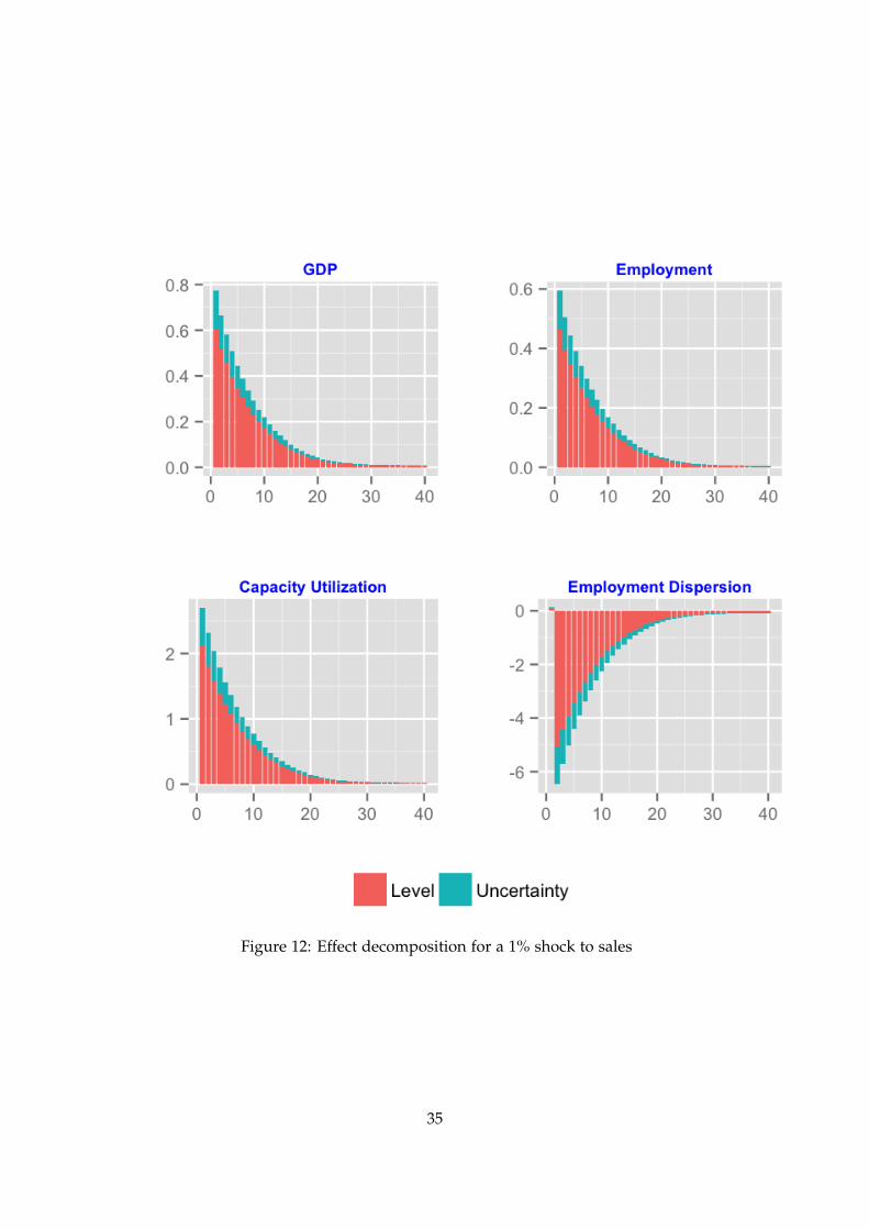
Figure 12: Effect decomposition for a 1% shock to sales

35

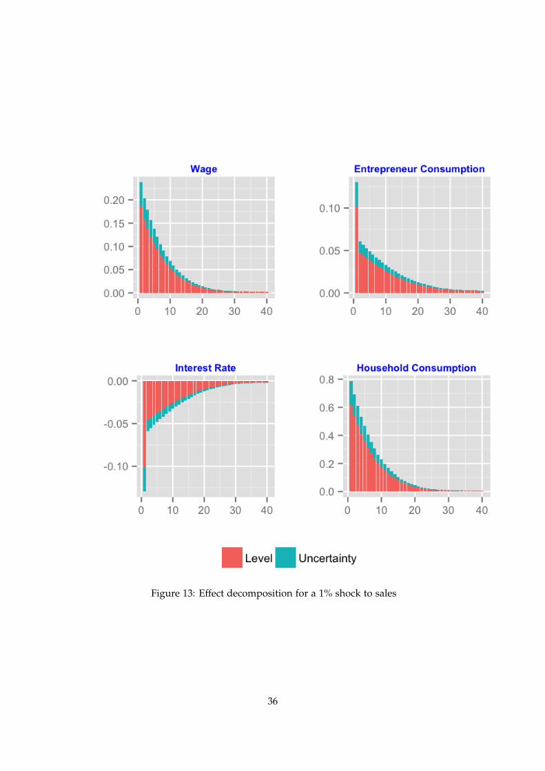
Figure 13: Effect decomposition for a 1% shock to sales

36

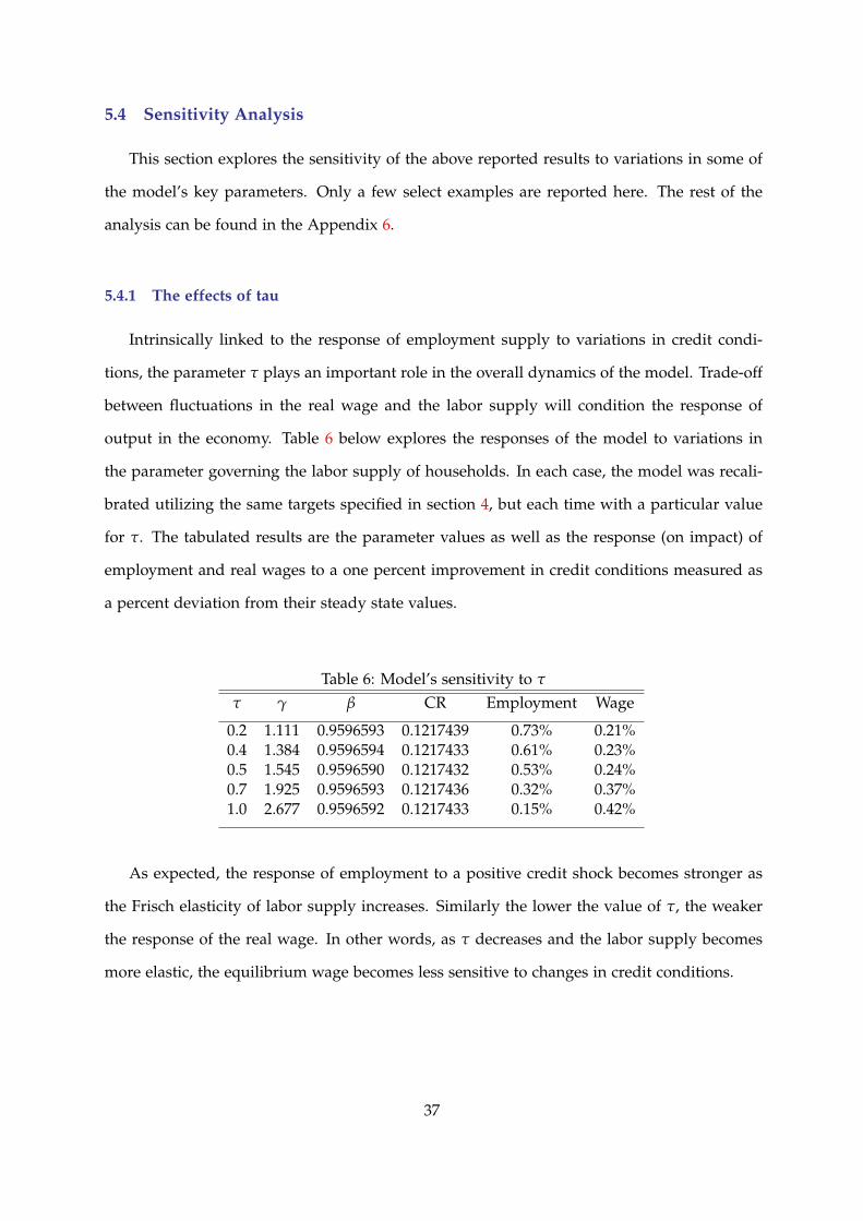
5.4 Sensitivity Analysis

This section explores the sensitivity of the above reported results to variations in some of

the model’s key parameters. Only a few select examples are reported here. The rest of the

analysis can be found in the Appendix 6.

5.4.1 The effects of tau

Intrinsically linked to the response of employment supply to variations in credit condi-

tions, the parameter τ plays an important role in the overall dynamics of the model. Trade-off

between fluctuations in the real wage and the labor supply will condition the response of

output in the economy. Table 6 below explores the responses of the model to variations in

the parameter governing the labor supply of households. In each case, the model was recali-

brated utilizing the same targets specified in section 4, but each time with a particular value

for τ. The tabulated results are the parameter values as well as the response (on impact) of

employment and real wages to a one percent improvement in credit conditions measured as

a percent deviation from their steady state values.

Table 6: Model’s sensitivity to τ

τ γ β CR Employment Wage

0.2 1.111 0.9596593 0.1217439 0.73% 0.21%0.4 1.384 0.9596594 0.1217433 0.61% 0.23%0.5 1.545 0.9596590 0.1217432 0.53% 0.24%0.7 1.925 0.9596593 0.1217436 0.32% 0.37%1.0 2.677 0.9596592 0.1217433 0.15% 0.42%

As expected, the response of employment to a positive credit shock becomes stronger as

the Frisch elasticity of labor supply increases. Similarly the lower the value of τ, the weaker

the response of the real wage. In other words, as τ decreases and the labor supply becomes

more elastic, the equilibrium wage becomes less sensitive to changes in credit conditions.

37

5.4.2 The effects of capacity utilization

The rate at which productive capacity is being used in the economy will be an important

factor governing its cross-sectional dynamics. Interestingly, the lower the steady state capacity

utilization rate, the greater the share of firms that will benefit from an improvement in credit

conditions and yet the worse the mean entrepreneur might end up being.

This happens because as credit expands and firms seek to increase their production, the

increase in labor demand puts pressure on the equilibrium wage. For those firms operat-

ing below y this increase in cost is still profit maximizing. Yet, for those already operating

at their maximum capacity, this increase represents a dent on their profits. Moreover, the

greater the share of firms initially operating below full capacity, the greater the increase in

labor demand and hence the greater the rise real wages. As firm’s operating costs rise, the

mean entrepreneur’s profit falls and so does his equilibrium consumption. Figure 14 plots

the model’s dynamic response to a one percent increase in θt, starting from a steady capacity

utilization rate of sixty percent.

On impact, there is a fifty percent stronger response of output than that described on Fig-

ure 11. In line with this reaction, equilibrium employment also rises more than in the baseline

specification. Similarly, employment dispersion drops as capacity utilization rates increase in

the economy. Overall most variables’ response seems consistent with the baseline results.

In terms of consumption, however, things change substantially. Since labor costs rise

sharply for all firms, the mean entrepreneur’s profit will fall. With less claims on final produc-

tion their consumption drops slightly, about 0.2 percent from steady state. With less profits,

entrepreneurs reduce their appetite for savings, causing bond prices to drop and consequently

inducing a rise in its yield. Households, on the other hand, are benefited by the strong in-

crease in wages and hours, although higher interest rates will act like a dent on their available

resources. Consequently their consumption rises, but less than in the baseline specification.

38

Figure 14: Effect decomposition for a 1% shock to θt

39

5.5 Extension: Persistent Demand Shocks

One of the assumptions present in the model’s baseline specification was that the idiosyn-

cratic disturbances faced by entrepreneurs presented no serial correlation. This afforded us

a tractable and intuitive closed form solution. However, there are reasons to believe that de-

mand fluctuations may in fact experience certain dependence over time.

Figure 15: Consumer Traffic and Business CycleSource: Own calculations based on ICSC data

To gain a deeper understanding of this assumption I utilize the consumer traffic diffusion

index from the International Consortium of Shopping Centers (ICSC). The diffusion index

is produced monthly by the ICSC from a survey of consumer traffic reported by shopping

center’s executives. Readings over 50 imply a general positive momentum in the number of

customers visiting shopping centers, while readings below 50 hint of a slowdown. The ad-

vantages of this data series over the ShopperTrak data is that it is available for a longer time

horizon. The disadvantage, however, is that since it constitutes an aggregated index, individ-

ual stores cannot be tracked across time. Figure 15 plots this alternative measure of consumer

traffic.

40

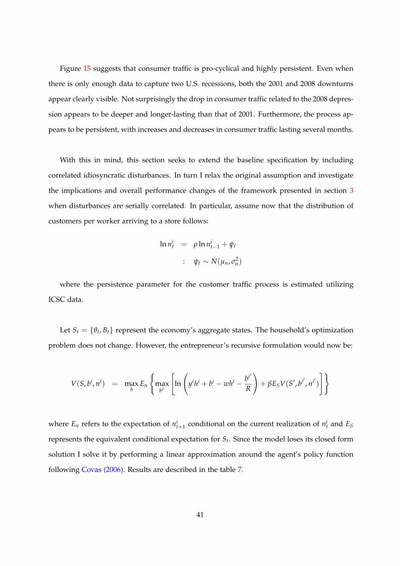
Figure 15 suggests that consumer traffic is pro-cyclical and highly persistent. Even when

there is only enough data to capture two U.S. recessions, both the 2001 and 2008 downturns

appear clearly visible. Not surprisingly the drop in consumer traffic related to the 2008 depres-

sion appears to be deeper and longer-lasting than that of 2001. Furthermore, the process ap-

pears to be persistent, with increases and decreases in consumer traffic lasting several months.

With this in mind, this section seeks to extend the baseline specification by including

correlated idiosyncratic disturbances. In turn I relax the original assumption and investigate

the implications and overall performance changes of the framework presented in section 3

when disturbances are serially correlated. In particular, assume now that the distribution of

customers per worker arriving to a store follows:

ln nit = ρ ln ni

t−1 + ψt

: ψt ∼ N(µn, σ2n)

where the persistence parameter for the customer traffic process is estimated utilizing

ICSC data.

Let St = θt, Bt represent the economy’s aggregate states. The household’s optimization

problem does not change. However, the entrepreneur’s recursive formulation would now be:

V(S, bi, ni) = maxh

En

max

bi′

[ln

(yihi + bi − whi − bi′

R

)+ βESV(S′, bi′ , ni′)

]

where En refers to the expectation of nit+1 conditional on the current realization of ni

t and ES

represents the equivalent conditional expectation for St. Since the model loses its closed form

solution I solve it by performing a linear approximation around the agent’s policy function

following Covas (2006). Results are described in the table 7.

41

Table 7: ResultsMoment Data Baseline Extension

Cross-sectional dispersion of employment 2.416 1.675 1.832Cross-sectional dispersion of sales 2.227 1.231 1.515Sales growth rate dispersion correl w/ cycle -0.388 -0.622 -0.533Emp growth rate dispersion correl w/ cycle -0.248 -0.586 -0.397Employment’s cross-sectional skewness -0.131 -0.222 -0.171Sale’s cross-sectional skewness -0.187 -0.272 -0.232Employment’s cross-sectional kurtosis 2.484 1.705 1.811Sales’s cross-sectional kurtosis 2.236 1.932 2.052

As can be seen from table 7, both the sales and employment dispersion growth rates ap-

pear countercyclical in all model specifications. This is in line with the data and implies that

the model’s results are qualitatively robust. Quantitatively, there is also a slight improvement

in the model’s capacity to match the data. The inclusion of serially correlated customer traffic

substantially improves the model’s effectiveness at at matching the desired moments.

42

6 Conclusion

In this study I have investigated the effects of fluctuations in uncertainty on aggregate

economic activity. In particular, I have done so contemplating the hypothesis that changes in

uncertainty are endogenous to the current state of the economy. The paper develops a gen-

eral equilibrium incomplete markets framework with heterogeneous firms that account for

the asymmetric fluctuations of the U.S. labor market and output. The fundamental property

of the model is that expansions and contractions in the economy are inititated by shifts in

aggregate credit conditions and these, in turn, may induce changes in uncertainty.

The model generates realistic volatility in aggregate employment and output. Moreover,

I have found that endogenous fluctuations in uncertainty may significant amplify the real

effects of first moment shocks. The uncertainty channel is shown to be able to propagate

approximately thirty percent of a level’s shock initial effect. The model also predicts that the

level of uncertainty varies with the business cycle. This is in line with what has been doc-

umented for the U.S. where every measure of uncertainty systematically falls in expansions

and rises during recessions.

I have also found that aggregate fluctuations will have effects on the cross-sectional dis-

persion of output and employment. This highlights the importance of taking into account

the risk tolerance of individual producers which is often washed away in aggregate figures.

Results confirm that the proper understanding of business cycles requires knowledge of the

cross-sectional distributions as well as the aggregate time-series. There is need for theories

that can explain not just the mean variation of consumption, output, and employment, but

also why the distribution of firm behavior changes considerably over the cycle and how this

may (or may not) matter in determining the amplitude of the cycle and the process of job

creation and destruction.

There are several extensions that might be useful to consider. The first one would be to add

capital to the framework. This would allow the model to provide insights into fluctuations in

43

investment, which is usually a more fundamental contributor to business cycle dynamics than

employment. Moreover, it could also shed light to the relationship between uncertainty and

asset allocation. Under a set-up with capital, the entrepreneur would now have two instru-

ments in which to save one yielding a safe but low return, and another one yielding a more

risky yet potentially more rewarding alternative.

Further, there are two potentially interesting extensions regarding the effects of uncertainty

on nominal variables. First, since the model is written in real terms, there is no explicit role

for monetary assets. Adding money to the study’s framework would allow for the exploration

of the effects of fluctuations in uncertainty on nominal shocks, as well as its effect on the role

of monetary policy. Additionally, the model could provide insights into the effectiveness of

monetary policy at different levels of economic uncertainty throughout the business cycle.

These extensions are left for future research efforts.

44

7 Appendix

7.1 Omitted Theoretical Proofs

Proposition 1. Individual labor demand is linear in financial wealth (bit), while consump-

tion and savings are linear in total assets (ait):

hit = φtbi

t

bit+1 = Rtβai

t

cit = (1− β)ai

t

Proof Proposition 1.

The recursive formulation of the entrepreneur’s problem presented in section 3.6 can also

be written in terms of the information available to the agent at the time of making a decision.

In turn, I define the following two stages or sub-problems:

Stage I:

Vt(θt, Bt, bit) = max

hit

Ent Vt(θt, Bt, ait)

s.t. : ait = (θtni

t − wt)hit + bi

t

Stage II:

Vt(θt, Bt, ait) = max

cit

[ln ct + βEθt+1Vt+1(θt+1, Bt+1, bit+1)]

s.t. : ait ≥ ci

t +bi

t+1

Rt

where Eθt+1 stands for the expectation of θt+1 conditional on the realization of θt.

In stage I the entrepreneur chooses its labor inputs aware of the extent of credit conditions,

yet uncertain about the level of demand that he will receive that period. In stage II, the

entrepreneur observes the realization of nit and allocates the end of period wealth between

consumption and savings. The stage I first order condition is:

45

δVt

δhit⇐⇒ Ent

[δVt

δait

δait

δhit

]= 0

The envelope condition δVt/δait = 1/ci

t is derived and then used in the expression above

to yield:

δVt

δhit⇐⇒ Ent

[θtni

t − wt

cit

]= 0

The stage II first order condition is:

δVt

δcit= 0 ⇐⇒ 1

cit+ βEnt

[Eθt+1

δVt+1

δbit+1

(−Rt)

]= 0

Substituting the relevant envelope condition, and denoting Et as conditional expectation given

the information set at time t yields the following Euler equation:

1ci

t= βEtRt

(1

cit+1

)

Next I prove Proposition 1 following a guess-and-verify approach. Begin by guessing the

following policy functions:

hit = φtbi

t (1)

bit+1 = Rtβai

t (2)

Replacing (2) in the stage II budget constraint

cit = ai

t −bi

t+1

Rt(3)

yields the policy function for consumption:

cit = (1− β)ai

t (4)

46

From the Euler equation (FOC of stage II) we have that

1ci

t= βRtEt

(1

cit+1

)

⇒ 1ai

t= βRtEt

(1

ait+1

)(5)

Combining the definition of ait and (1) yields

ait+1 = [(θt+1ni

t+1 − wt+1)φt+1 + 1]bit+1 (6)

which implies that (5) can be written as:

1ai

t=

(βRt

bit+1

)Et

(1

1 + (θt+1nit+1 − wt+1)φt+1

)

⇒ 1 = Et

(1

1 + (θt+1nit+1 − wt+1)φt+1

)(7)

For the proof to be complete I need to verify that (7) satisfies the problem’s FOCs:

Et

[θtni

t − wt

(θtnit − wt)φt + 1

]= 0 (8)

In turn, from (7)

Et

[1

1 + (θtnit − wt)φt

]− 1 = 0 (9)

⇒ Et

[1− 1− (θtni

t − wt)φ

1 + (θtnit − wt)φt

]= 0

⇒ (−φ)Et

[θtni

t − wt

1 + (θtnit − wt)φt

]= 0

⇒ Et

[θtni

t − wt

(θtnit − wt)φt + 1

]= 0 (10)

which satisfies (8).

47

7.2 Aggregate Measures

For this economy, aggregate real income will equal the profits of the entrepreneurs and

the labor income of the representative household. In turn:

Yt =∫(yi

t − wt)hit dF(i) + wtht (11)

=∫

yith

it dF(i)−

∫wthi

t dF(i) + wtht

=∫

yith

it dF(i)

In terms of real consumption:

ce,it dF(i) = (yi

t − wt)hit + bi

t −bi

t+1

Rt

⇒∫

ce,it dF(i) =

∫(yi

t − wt)hit dF(i) +

∫bi

t dF(i)−∫ bi

t+1

RtdF(i)

This implies that the aggregate consumption of entrepreneurs can be written as:

CEt = Yt − wtht + be

t −be

t+1

Rt

and aggregate consumption of the households as

CHt = wtht +

bHt+1

Rt− bH

t

Hence total consumption in the economy would be equal to:

CEt + CH

t = Yt − wtht + bet −

bet+1

Rt+ wtht +

bHt+1

Rt− bH

t

= Yt + bet −

bet+1

Rt+

bHt+1

Rt− bH

t

= Yt

which is the total income/production described by expression 11.

48

7.3 Alternatives Measures of Uncertainty

Figure 16: Disagreement amongst professional forecasters. The figure above plots the crosssectional dispersion in private sector forecasts over the business cycle. The data comes fromthe Federal Reserve Bank of Philadelphia’s survey of professional forecasters from 1968Q4 -2014Q3 for the first four variables and 1981Q3 - 2014Q3 for the remaining two. Beginningfrom top left we have the forecasts for Real GDP, the Price Deflator, Industrial Production, theUnemployment rate, Real Consumption and Non-residential fixed investment. In times of higheruncertainty forecasts become less precise and dispersion amongst predictions increases. Notsurprisingly, recessions tend to be periods of greatest disagreement amongst forecasters.

49

7.4 Evidence of Corporate Lending

In the framework introduced in Section 3 resources would, in equilibrium, flow from the

entrepreneurs to the households sector. At first this result might seem like an odd feature of

the model. However, in the U.S., the private corporate sector has been a net lender since the

beginning of the 2000’s as seen in figure 17. The only exception to date has been the year

2008 at the height of the Big Recession, when the financial assets held by most corporations

dropped in value.

Figure 17: Net Financial Assets in the nonfinancial business sector as a percentage of totalnonfinancial assets. Source: Federal Reserve Flow of Funds Report.

Interestingly the reversal from net borrower to lender has so far only occurred in the U.S.

Corporate sector, and not in the Noncorporate one. The evidence reported on the figure above

shows that a large fraction of the business sector is self-financing and no longer dependent on

outside sources. And even when the aggregate figures may mask some firm level heterogene-

ity, they do paint a general picture of the evolution of the overall trend across time.

50

7.5 About ShopperTrak data

Founded in 1989 and headquartered in Chicago, Illinois; ShopperTrak Corporation is the

world’s largest retail traffic counter. The company provides shopper insights and analytics

solutions to improve retail profitability and effectiveness. ShopperTrak helps companies iden-

tify, understand, and maximize their total shopper conversion rate (the percentage of shoppers

who actually purchase something) and improves store performance through shopper behavior

insights. It also helps retailers with solutions for store traffic counting, interior analytics, and

industry benchmarking; and provides unique data benchmark tools that help retailers under-

stand their performance in context of the market. ShopperTrak is the leader in its industry

and the only one to provide an end-to-end service: from device installation to data analysis.

The company serves major brands, retailers, mall owners, and financial institutions. Table 8

provides a small selection of its customer base.

ShopperTrak utilizes propiertary technology to analyze and monitor customer traffic. Its

fifth-generation device, called the Orbit, is smart enough to detect shoppers who enter side-

by-side or in groups, distinguish children from adults and ignore shopping carts or strollers.

Figure 18 provides a few examples of this technology. All images were taken from local stores

in Santa Monica, CA.

Table 8: ShopperTrak ClientsApparel Home Improvement Technology Food

GAP Inc. (Old Navy, GAP, BR) Home Depot Apple Inc. GodivaCrocs Lowe’sVictorias Secret Crate & BarrelPayless ShoesAmerican Eagle OutfittersJ. CrewJourneysThomas Sabo

Source: ShopperTrak’s website and specialized press

51

Figure 18: ShopperTrak’s technology

52

References

Andrew B Abel. Optimal investment under uncertainty. The American Economic Review, pages

228–233, 1983.

Andrew B Abel and Janice C Eberly. Optimal investment with costly reversibility. The Review

of Economic Studies, 63(4):581–593, 1996.

S Rao Aiyagari. Uninsured idiosyncratic risk and aggregate saving. The Quarterly Journal of

Economics, pages 659–684, 1994.

George-Marios Angeletos. Uninsured idiosyncratic investment risk and aggregate saving.

Review of Economic Dynamics, 10(1):1–30, 2007.

George-Marios Angeletos and Laurent-Emmanuel Calvet. Idiosyncratic production risk,

growth and the business cycle. Journal of Monetary Economics, 53(6):1095–1115, 2006.

George-Marios Angeletos and Vasia Panousi. Financial integration, entrepreneurial risk and

global dynamics. Journal of Economic Theory, 146(3):863–896, 2011.

Cristina Arellano. Default risk and income fluctuations in emerging economies. The American

Economic Review, pages 690–712, 2008.

Cristina Arellano, Yan Bai, and Patrick Kehoe. Financial markets and fluctuations in uncer-

tainty. Federal Reserve Bank of Minneapolis Working Paper, 2010.

Yavuz Arslan, Ashhan Atabek, and Saygin Sahinoz. Expectation errors, uncertainty and eco-

nomic activity. Bank of Turkey mimeo, 2011.

Rüdiger Bachmann and Christian Bayer. ‘wait-and-see’business cycles? Journal of Monetary

Economics, 60(6):704–719, 2013.

Rüdiger Bachmann and Christian Bayer. Investment dispersion and the business cycle. The

American Economic Review, 104(4):1392–1416, 2014.

Rudiger Bachmann and Giuseppi Moscarini. Business cycles and endogenous uncertainty.

Yale University mimeo, 2011.

53

Rüdiger Bachmann, Steffen Elstner, and Eric R Sims. Uncertainty and economic activity:

Evidence from business survey data. American Economic Journal: Macroeconomics, 5(2):217–

249, 2013.

Yan Bai, Jose-Victor Rios-Rull, and Kjetil Storesletten. Demand shocks as productivity shocks.

Federal Reserve Board of Minneapolis, 2012.

Scott Baker and Nicholas Bloom. Does uncertainty drive business cycles? using disasters as

natural experiments. NBER Working Paper, 2011.

Scott R Baker, Nicholas Bloom, and Steven J Davis. Measuring economic policy uncertainty.

Stanford University mimeo, 2012.

Ravi Bansal and Amir Yaron. Risks for the long run: A potential resolution of asset pricing

puzzles. The Journal of Finance, 59(4):1481–1509, 2004.

Susanto Basu and Brent Bundick. Uncertainty shocks in a model of effective demand. NBER

Working Paper, 2012.

Geert Bekaert, Marie Hoerova, and Marco Lo Duca. Risk, uncertainty and monetary policy.

Journal of Monetary Economics, 60(7):771–788, 2013.

Truman Bewley. The permanent income hypothesis: A theoretical formulation. Journal of

Economic Theory, 16(2):252–292, 1977.

Nicholas Bloom. The impact of uncertainty shocks. Econometrica, 77(3):623–685, 2009.

Nicholas Bloom. Fluctuations in uncertainty. Technical report, National Bureau of Economic

Research, 2013.

Nicholas Bloom, Max Floetotto, Nir Jaimovich, Itay Saporta-Eksten, and Stephen J Terry. Re-

ally uncertain business cycles. NBER Working Paper No 18245, 2012.

Nick Bloom, Stephen Bond, and John Van Reenen. Uncertainty and investment dynamics. The

Review of Economic Studies, 74(2):391–415, 2007.

Benjamin Born and Johannes Peifer. Policy risk and the business cycle. Journal of Monetary

Economics, 2014.

54

Giovanni Caggiano, Efrem Castelnuovo, and Nicolas Groshenny. Uncertainty shocks and

unemployment dynamics in us recessions. Journal of Monetary Economics, 2014.

Dario Caldara, Cristina Fuentes-Albero, Simon Gilchrist, and E Zakrajsek. The macroeconomic

impact of financial and uncertainty shocks. FRB Working Paper, 2014.

Ambrogio Cesa-Bianchi, M. Hashem Pesaran, and Alessandro Rebucci. Uncertainty and eco-

nomic activity: A global perspective. CESIFO Working Paper 4736, 2014.

Francisco Covas. Uninsured idiosyncratic production risk with borrowing constraints. Journal

of Economic Dynamics and Control, 30(11):2167–2190, 2006.

Steven J Davis, R Jason Faberman, and John Haltiwanger. The flow approach to labor markets:

New data sources and micro-macro links. Journal of Economic Perspectives, 20:3–26, 2006.

Ryan Decker, Pablo D’Erasmo, and Hernan J Moscoso Boedo. Market exposure and endoge-

nous firm volatility over the business cycle. FRB of Philadelphia Working Paper, 2014.

Stephanie Denis and Prakash Kannan. The impact of uncertainty shocks on the uk economy.

IMF Working Paper, 2013.

Pablo N D’Erasmo and Hernan J Moscoso Boedo. Intangibles and endogenous firm volatility

over the business cycle. University of Virginia mimeo, 2011.

Pablo Fajgelbaum, Edouard Schaal, and Mathieu Taschereau-Dumouchel. Uncertainty traps.

NBER Working Paper, 2014.

J Fernández-Villaverde, P Guerrón-Quintana, J Rubio-Ramirez, and M Uribe. Risk matters:

The real effects of stochastic volatility. American Economic Review, 2011.

Jesús Fernández-Villaverde, Pablo A Guerrón-Quintana, Keith Kuester, and Juan Rubio-

Ramírez. Fiscal volatility shocks and economic activity. NBER Working Paper, 2013.

Ana Fostel and John Geanakoplos. Why does bad news increase volatility and decrease lever-

age? Journal of Economic Theory, 147(2):501–525, 2012.

Simon Gilchrist and John C Williams. Investment, capacity, and uncertainty: a putty–clay

approach. Review of Economic Dynamics, 8(1):1–27, 2005.

55

Simon Gilchrist, Jae W Sim, and Egon Zakrajšek. Uncertainty, financial frictions, and invest-

ment dynamics. Technical report, NBER Working Paper No. 20038, 2014.

Luigi Guiso and Giuseppe Parigi. Investment and demand uncertainty. Quarterly Journal of

Economics, pages 185–227, 1999.

Kyle F. Herkenhoff. The impact of consumer credit access on unemployment. University of

California Los Angeles mimeo, 2013.

Chris Higson, Sean Holly, and Paul Kattuman. The cross-sectional dynamics of the us business

cycle: 1950-1999. Journal of Economic Dynamics and Control, 26(9):1539–1555, 2002.

Chris Higson, Sean Holly, Paul Kattuman, and Stylianos Platis. The business cycle, macroe-

conomic shocks and the cross-section: The growth of uk quoted companies. Economica, 71

(282):299–318, 2004.

Mark Huggett. The risk-free rate in heterogeneous-agent incomplete-insurance economies.

Journal of economic Dynamics and Control, 17(5):953–969, 1993.

Mark Huggett. The one-sector growth model with idiosyncratic shocks: Steady states and

dynamics. Journal of monetary economics, 39(3):385–403, 1997.

Urban Jermann and Vincenzo Quadrini. Macroeconomic effects of financial shocks. American

Economic Review, 102(1), 2012.

Matthias Kehrig. The cyclicality of producitivity dispersion. University of Texas at Austin mimeo,

2011.

Bryan Kelly, Hanno Lustig, and Stijn Van Nieuwerburgh. Firm volatility in granular networks.

NBER Working Paper, 2013.

Miklos Koren and Silvana Tenreyro. Volatility and development. The Quarterly Journal of

Economics, pages 243–287, 2007.

Per Krusell and Anthony A Smith. On the welfare effects of eliminating business cycles.

Review of Economic Dynamics, 2(1):245–272, 1999.

56

Per Krusell and Anthony A Smith, Jr. Income and wealth heterogeneity in the macroeconomy.

Journal of Political Economy, 106(5):867–896, 1998.

John V Leahy and Toni M Whited. The effect of uncertainty on investment: Some stylized

facts. Journal of Money, Credit and Banking, 28:64–83, 1996.

Sylvain Leduc and Zheng Liu. Uncertainty shocks are aggregate demand shocks. Federal

Reserve Bank of San Francisco Working Paper, 10, 2012.

Césaire A Meh and Vincenzo Quadrini. Endogenous market incompleteness with investment

risks. Journal of Economic Dynamics and Control, 30(11):2143–2165, 2006.

Anna Orlik and Laura Veldkamp. Understanding uncertainty shocks and the role of the black

swan. NYU mimeo, 2013.

Nicolas Petrosky-Nadeau and Etienne Wasmer. Macroeconomic dynamics in a model of

goods, labor and credit market frictions. Carnegie Mellon University mimeo, 2011.

Vincenzo Quadrini. The importance of entrepreneurship for wealth concentration and mobil-

ity. Review of income and Wealth, 45(1):1–19, 1999.

Vincenzo Quadrini. Entrepreneurship, saving, and social mobility. Review of Economic Dynam-

ics, 3(1):1–40, 2000.

Vincenzo Quadrini. Bank liabilities channel. University of Southern California mimeo, 2014.

Felix Reichling and Charles Whalen. Review of estimates of the frisch elasticity of labor

supply. Congressional Budget Office Working Paper, 2012.

Chiara Scotti and Vivian Z Yue. Surprise and uncertainty indexes: real-time aggregation of

real-activity macro surprises. FRB Working Paper, 2013.

LC Stein and EC Stone. The effect of uncertainty on investment, hiring, and r&d: Causal

evidence from equity options. Stanford University mimeo, 2011.

Joseph S Vavra. Inflation dynamics and time-varying volatility: New evidence and an ss

interpretation. NBER Working Paper, 2013.

57