demand flexibility in supply chain planning
TRANSCRIPT


SpringerBriefs in Optimization
For further volumes:www.springer.com/series/8918
Joseph Geunes
Demand Flexibilityin Supply ChainPlanning

Joseph GeunesIndustrial and Systems EngineeringUniversity of FloridaGainesville, FLUSA
ISSN 2190-8354 e-ISSN 2191-575XSpringerBriefs in OptimizationISBN 978-1-4419-9346-5 e-ISBN 978-1-4419-9347-2DOI 10.1007/978-1-4419-9347-2Springer New York Dordrecht Heidelberg London
Library of Congress Control Number: 2012933121
Mathematics Subject Classification (2010): 60C05, 60A10, 90B15, 90B99
© Joseph Geunes 2012All rights reserved. This work may not be translated or copied in whole or in part without the writtenpermission of the publisher (Springer Science+Business Media, LLC, 233 Spring Street, New York,NY 10013, USA), except for brief excerpts in connection with reviews or scholarly analysis. Use inconnection with any form of information storage and retrieval, electronic adaptation, computer software,or by similar or dissimilar methodology now known or hereafter developed is forbidden.The use in this publication of trade names, trademarks, service marks, and similar terms, even if they arenot identified as such, is not to be taken as an expression of opinion as to whether or not they are subjectto proprietary rights.
Printed on acid-free paper
Springer is part of Springer Science+Business Media (www.springer.com)

For Paul & Vicki Geunesand Sherry, Eric, and Brett
Preface
The goal of this book is to codify ideas and results from a specific segment of thesupply chain operations planning literature that has developed over the past fewdecades. This segment of the literature draws on the tools of operations research inorder to characterize optimal solutions to problems that seek to efficiently matcha producer’s supply output with the demands or requirements of a set of customersand/or markets. More specifically, we will emphasize contexts in which the producerhas some control over both supply and demand, i.e., situations in which some degreeof flexibility in demand exists from the producer’s point of view.
The evolution of the operations literature in the past half century has by andlarge focused on managing (or minimizing) costs while attempting to meet someexternal party’s target output requirements. This external party often corresponds toa marketing group within the same firm, whose responsibilities include setting pricesand estimating the resulting customer demand levels, in effect, determining optimaldemand levels with respect to some objective. Understanding how price influencesdemand for a good, and thus, what constitutes an optimal set of demand levels,requires some knowledge of how customers will respond to one of the product’scritical characteristics (in this case, price). Defining the way in which customerswill respond to price in the aggregate is analogous to characterizing the degree offlexibility that exists in demand as a function of price. Customer flexibility oftenexists along numerous product dimensions in addition to price (e.g., product sizes,delivery quantities, delivery lead times), many of which are directly controllable viaproduction and distribution operations.
In addition to inherent customer flexibility with respect to product characteris-tics, a supplier or producer often has discretion as to which customers, demands,or markets it will satisfy with its product(s). This discretion provides an additionalsource of flexibility in planning by permitting the producer to accept or decline cer-tain customers or markets.
Models for operations planning have typically treated demands as fixed, exoge-nous parameters, based on predetermined price levels and other fixed product char-acteristics. This corresponds to a sequential decision making process in which dif-ferent decisions that ultimately combine to determine profitability are made sepa-rately. That is, marketing and sales groups essentially estimate the demand levels for
vii

viii Preface
products containing specific characteristics offered at specific prices, and operationsis tasked with meeting the implied demands at the lowest delivered cost. An alter-native view, which serves as the focus of this book, treats demand (and/or revenue)as dependent on key product-characteristic and customer-acceptance decisions thatare made by the producer. This leads to new classes of operations planning modelsthat effectively treat demand levels as decision variables within the planning model.The resulting models then determine the optimal production and demand levels, i.e.,the most efficient match between the supply process and the inherently flexible de-mands. This book thus brings together several operations research based planningmodels that share this alternative view of sales and operations planning. As the fi-nal part of the book indicates, the models presented provide a foundation for bothadapting a wealth of existing problems to this paradigm and for its extension andgeneralization to even broader classes of decision problems.
Joseph GeunesGainesville, FL, USA

Acknowledgements
The majority of the contents of this book are the product of collaborative researchover the past decade with numerous colleagues and collaborators who appear in thevarious references. Many of the key contributions and ideas presented throughoutthe book are attributable to these collaborators, and this book is an attempt to distillthese contributions into a manageable and digestible form. I am forever indebtedto my teachers, colleagues, and students, without whom this book and the researchon which it is based could not exist. I would first like to acknowledge and thankAnant Balakrishnan, who instilled research standards which, despite eluding mygrasp, serve as a goal to which I continue to strive. My primary collaborator (andfriend) over the past decade has been Edwin Romeijn, who has taught me as muchas anyone I have encountered. I only hope he has found our collaboration to be halfas beneficial as have I. I would like to acknowledge the debt I owe to my departmentchairs Don Hearn and Joe Hartman for the support and freedom they have provided.I would also like to acknowledge several of the key contributors of important de-velopments contained within this work, in particular, Wilco van den Heuvel, WeiHuang, Erhun Kundakcioglu, Retsef Levi, Tom Sharkey, Max Shen, David Shmoys,and Albert Wagelmans. In addition to these colleagues, I was fortunate to work withseveral insightful and energetic students on the problems contained in this book,including Semra Agralı, Ismail Bakal, Yasemin Merzifonluoglu, Chase Rainwater,and Kevin Taaffe. Finally, I would like to acknowledge the support provided by theNational Science Foundation (grants #DMI-0322715 and #CMMI-0927930).
ix

Contents
Part I Supply Chain Operations Models with Demand Shaping
1 Scope of Problem Coverage and Introduction . . . . . . . . . . . . . 31.1 Scope and Preliminaries . . . . . . . . . . . . . . . . . . . . . . . 31.2 Overview of Foundational Models . . . . . . . . . . . . . . . . . . 4
1.2.1 The Economic Order Quantity (EOQ) Model . . . . . . . . 41.2.2 The Newsvendor Problem . . . . . . . . . . . . . . . . . . 61.2.3 The Economic Lot Sizing Problem (ELSP) . . . . . . . . . 71.2.4 The Knapsack Problem (KP) . . . . . . . . . . . . . . . . 91.2.5 The Generalized Assignment Problem (GAP) . . . . . . . 111.2.6 The Facility Location Problem (FLP) . . . . . . . . . . . . 12
References . . . . . . . . . . . . . . . . . . . . . . . . . . . . . . . . . 13
2 Production and Inventory Planning Models with Demand Shaping . 152.1 EOQ Models with Pricing . . . . . . . . . . . . . . . . . . . . . . 152.2 The Newsvendor Problem with Pricing and Demand Shaping . . . 162.3 Lot Sizing with Pricing . . . . . . . . . . . . . . . . . . . . . . . 182.4 Knapsack Problems with Nonlinear Objectives . . . . . . . . . . . 202.5 Location and Assignment Problems with Flexible Demand . . . . . 22References . . . . . . . . . . . . . . . . . . . . . . . . . . . . . . . . . 23
Part II Production Planning with Demand Flexibility
3 EOQ-Type Models with Demand Selection . . . . . . . . . . . . . . . 273.1 Unconstrained EOQ Problems with Market Choice . . . . . . . . . 27
3.1.1 Standard EOQ with Market Choice . . . . . . . . . . . . . 273.1.2 The EPQ Problem with Market Choice . . . . . . . . . . . 29
3.2 EOQMC Problems with Constraints . . . . . . . . . . . . . . . . . 303.2.1 Demand Rate Constraints . . . . . . . . . . . . . . . . . . 303.2.2 Batch Size Constraints . . . . . . . . . . . . . . . . . . . . 31
References . . . . . . . . . . . . . . . . . . . . . . . . . . . . . . . . . 32
xi
xii Contents
4 Single-Period Stochastic Inventory Planning with Demand Selection 334.1 The Selective Newsvendor Problem . . . . . . . . . . . . . . . . . 334.2 The Basic SNP . . . . . . . . . . . . . . . . . . . . . . . . . . . . 334.3 The SNP with Market Effort . . . . . . . . . . . . . . . . . . . . . 34
4.3.1 Market Variance Independent of Market Effort . . . . . . . 354.3.2 Market Variance Dependent on Market Effort . . . . . . . . 35
4.4 The SNP with Limited Market Resources . . . . . . . . . . . . . . 364.5 The SNP with Pricing . . . . . . . . . . . . . . . . . . . . . . . . 37
4.5.1 Equal Market Prices . . . . . . . . . . . . . . . . . . . . . 374.5.2 SNP with Market Price Discrimination . . . . . . . . . . . 39
References . . . . . . . . . . . . . . . . . . . . . . . . . . . . . . . . . 39
5 Dynamic Lot Sizing with Demand Selection and the Pricing Analog . 415.1 Demand Selection Problem Definition . . . . . . . . . . . . . . . 415.2 Dual Ascent Solution Algorithm . . . . . . . . . . . . . . . . . . 435.3 Shortest Path Solution Approach . . . . . . . . . . . . . . . . . . 455.4 Interpretation of the DSP as a Pricing Problem . . . . . . . . . . . 465.5 Capacitated Versions . . . . . . . . . . . . . . . . . . . . . . . . . 47References . . . . . . . . . . . . . . . . . . . . . . . . . . . . . . . . . 50
6 Dynamic Lot Sizing with Market Selection . . . . . . . . . . . . . . . 516.1 Market Selection Problem Definition . . . . . . . . . . . . . . . . 51
6.1.1 MSP Problem Complexity . . . . . . . . . . . . . . . . . . 536.1.2 MSP Approximability . . . . . . . . . . . . . . . . . . . . 546.1.3 Polynomially Solvable Special Cases . . . . . . . . . . . . 576.1.4 Heuristic Solution Methods . . . . . . . . . . . . . . . . . 59
References . . . . . . . . . . . . . . . . . . . . . . . . . . . . . . . . . 60
Part III Supply Chain Network Planning with Demand Flexibility
7 Assignment and Location Problems in Supply Chains . . . . . . . . 637.1 Demand Selection Problems . . . . . . . . . . . . . . . . . . . . . 63
7.1.1 The GAP with Demand Selection . . . . . . . . . . . . . . 637.1.2 The FLP with Demand Selection . . . . . . . . . . . . . . 64
7.2 Problems with Demand Specification Flexibility . . . . . . . . . . 657.2.1 The GAP with Demand Specification Flexibility . . . . . . 667.2.2 The FLP with Demand Specification Flexibility . . . . . . 69
References . . . . . . . . . . . . . . . . . . . . . . . . . . . . . . . . . 70
8 Branch-and-Price Decomposition for Assignment and LocationProblems . . . . . . . . . . . . . . . . . . . . . . . . . . . . . . . . . 718.1 Branch-and-Price Approach . . . . . . . . . . . . . . . . . . . . . 718.2 Branch-and-Price for Supply Chain Planning Problems . . . . . . 74
8.2.1 The Continuous-Time Single-Sourcing Problem . . . . . . 748.2.2 Single-Period Demand Allocation with Uncertainty . . . . 758.2.3 Integrated Facility Location and Production Planning . . . 778.2.4 The GAP and FLP with Flexible Demands . . . . . . . . . 79
References . . . . . . . . . . . . . . . . . . . . . . . . . . . . . . . . . 81

Contents xiii
Part IV Research Directions and Modeling Challenges
9 Research Challenges in Supply Chain Planning with Flexible Demand 859.1 Dimensions of Demand Flexibility Modeling . . . . . . . . . . . . 859.2 Model Limitations . . . . . . . . . . . . . . . . . . . . . . . . . . 869.3 Limitations of Branch-and-Price Decomposition . . . . . . . . . . 879.4 Further Generalizations and Approximation Algorithms . . . . . . 88References . . . . . . . . . . . . . . . . . . . . . . . . . . . . . . . . . 90

Part ISupply Chain Operations Models
with Demand Shaping

Chapter 1Scope of Problem Coverage and Introduction
Abstract This chapter begins with an introduction to the book’s scope and prelim-inary concepts applied throughout the book. We then present a set of basic, founda-tional, and classical models from the operations planning literature that serve as theunderpinning of the work presented throughout the book. These models include theeconomic order quantity (EOQ), the newsvendor problem, the economic lot-sizingproblem (ELSP), the knapsack problem (KP), the generalized assignment problem(GAP), and the facility location problem (FLP). The main results presented laterin this book generalize these classical models to account for a planner’s ability toinfluence demands, which have traditionally served as fixed parameters in thesefoundational models.
1.1 Scope and Preliminaries
The work in this book generalizes several of the most fundamental and classicalmodels for production and inventory planning. These include the economic orderquantity (EOQ), the newsvendor problem, the economic lot-sizing problem (ELSP),the knapsack problem (KP), the generalized assignment problem (GAP), and the fa-cility location problem (FLP). Each of these models involves a very specific setof assumptions, which we will specify when introducing the associated model.Each model represents an abstraction with respect to some practical problem thatis broadly applicable to entities that produce and/or stock consumer goods. This ab-straction results in an idealized version of the associated real-world problem and,thus, one is unlikely to find that the required assumptions hold precisely in anypractical setting. Despite this, these models are powerful for their approximation ofreality and because they mathematically formalize important relationships amongthe key parameters and decision factors that combine to determine the economicperformance of the system being modeled. This book will, therefore, present eachmodel and its assumptions without providing strenuous arguments as to the degreeto which these assumptions provide an effective approximation for any particularpractical setting.
For ease of exposition, this book will also focus on the single-product version ofthe models in question. While multiple-product generalizations often follow basedon a straightforward analysis, these generalizations tend to detract from the central
J. Geunes, Demand Flexibility in Supply Chain Planning,SpringerBriefs in Optimization,DOI 10.1007/978-1-4419-9347-2_1, © Joseph Geunes 2012
3

4 1 Scope of Problem Coverage and Introduction
theme of modeling sources of demand flexibility. For the single-product version ofa problem, we will essentially draw on three techniques to model a producer’s abil-ity to shape demand. The first of these techniques involves the ability to explicitlyselect a subset from some set of potential demands. We will refer to this techniqueas demand selection. We will refer to cases in which demand selection requires se-lecting all or none of a time-phased vector of demands as market selection. Thesecond technique implicitly selects demands as a result of the dependence of de-mand on price. In this approach, selecting a demand level is equivalent to selectinga price level, assuming a one-to-one correspondence between price and demand inany planning period. The third technique we will explore may be characterized as aform of demand sizing. This method permits selecting the level, quantity, or size atwhich each demand will be satisfied, within some prespecified upper and lower lim-its. Observe that this concept of demand sizing generalizes demand selection whenthe prespecified lower limit equals zero. That is, choosing a size of zero under thedemand sizing technique corresponds to a decision to not select a given demand,whereas choosing a positive size corresponds to selecting the demand for satisfac-tion.
1.2 Overview of Foundational Models
This section describes the basic models that serve as a basis for our explorationof operations models that incorporate demand flexibility. Each of the following sixsubsections provides a brief definition of a model that will be generalized in a laterchapter.
1.2.1 The Economic Order Quantity (EOQ) Model
The economic order quantity (EOQ) model serves as the oldest quantitative modelfor production and inventory planning [8]. Despite its simplicity and high degreeof abstraction, it remains widely used today, as it elegantly captures perhaps themost critical tradeoff inherent in inventory planning contexts between fixed ordercosts and inventory holding costs. We next provide an overview of the EOQ modelassumptions and main results. For an in-depth derivation and analysis of the EOQmodel, please see [9].
The EOQ model considers a single stage of inventory that stocks a single productwith a constant and continuous demand rate of D units per unit time that will persistinfinitely far into the future. The planner wishes to stock the item in order to ensurethat all demands are met from stock as they occur. This is possible because thedemand rate is deterministic and the stage replenishes from a supply source witha known and fixed (and finite) delivery lead time and with no capacity limit onthe amount it can supply. Any time the stage orders a quantity of Q units from thesupply source, all Q units are delivered after the fixed lead time. The planner pays C

1.2 Overview of Foundational Models 5
dollars for each unit ordered and also pays a fixed order cost of S dollars each time areplenishment order is placed. The planner also accrues a holding cost for each unitheld in inventory of H dollars per unit per unit time. The planner wishes to minimizethe average cost per unit time over the infinite horizon while meeting all demandson time. It is straightforward to show that because all costs are time invariant, as isthe demand rate, the planner’s optimal policy requires periodically ordering batchesof constant size (Q), and timing these replenishment orders to arrive precisely at thepoint in time at which the current on-hand inventory will reach zero. The averagecost per unit time as a function of the order quantity Q, which we denote by AC(Q),can be written as
AC(Q) = CD + SD
Q+ H
Q
2. (1.1)
The first term in (1.1) captures the average variable purchase cost per unit time,while the second and third terms correspond to the average fixed order cost per unittime and the average holding cost per unit time, respectively. It is straightforwardto show that AC(Q) is strictly convex in Q for all Q > 0, which implies that thefollowing stationary point serves as a strict global minimum for (1.1) among allpositive Q values:
Q∗ =√
2SD
H. (1.2)
Equation (1.2) is referred to as the economic order quantity and it captures the crit-ical tradeoff between fixed order costs and holding costs. A high relative value ofthe fixed order cost S leads to a large batch size, which increases the time betweenorders. Conversely, a high relative value of the holding cost H reduces the batchsize, which leads to a lower average inventory level. It is more than an interestingmathematical curiosity that, at the optimal (EOQ) batch size, the average setup costper unit time is exactly matched to the average holding cost per unit time, i.e.,
SD
Q∗ = HQ∗
2=
√SDH
2. (1.3)
This result has motivated numerous heuristic solution approaches for more complexinventory planning problems in an attempt to match average fixed order costs andholding costs per unit time as closely as possible (see [9]). As a result of (1.3), thevalue of AC(Q) at the EOQ can be written compactly as
AC(Q∗) = CD + √2SDH. (1.4)
The above equation (1.4) will come into play again in Chap. 3 when we considerEOQ-type models with demand selection.
Before concluding this section, we note that the above equations can easily begeneralized to account for settings in which the batch of size Q is not delivered allat one instant following a fixed lead time, but is instead accumulated at a finite rate.In particular, if inventory is accumulated at a rate of P units per unit time (where
6 1 Scope of Problem Coverage and Introduction
we must assume that P ≥ D in order to be able to keep up with demand), thenwe can simply replace each instance of the parameter H in Eqs. (1.1)–(1.4) withH ′ = 1 − D/P and all of the results we have discussed remain valid. The resultingmodel is often referred to as the EOQ problem with a finite production rate, orsimply as the Economic Production Quantity (EPQ) model. While the EOQ modeltends to be more appropriate for an inventory stage that orders in batches from anexternal supplier, the EPQ model tends to apply more readily to internal productionenvironments when production contributes to inventory at a finite rate.
1.2.2 The Newsvendor Problem
The newsvendor problem is perhaps the simplest stochastic model for inventoryplanning. This problem considers a single planning period with uncertain demand.Demand in the period is therefore a random variable, which we denote as xD , withan associated probability density function (pdf) of f (xD) and cumulative distri-bution function (cdf) F(xD) (our approach will assume that demand in the singleperiod can be effectively modeled using a continuous probability distribution withmean μD and standard deviation σD). The planner stocks Q units in anticipation ofthe period’s demand, where each unit comes at a procurement cost of C per unit.Stock is sold at a fixed unit price p. Any remaining stock at the end of the period isassessed a cost of H per unit, where a negative value of H corresponds to a salvagevalue and a positive value may be viewed as a disposal cost or, more generically,a holding cost. If demand exceeds the stock level Q, each shortage is assessed apenalty cost of B per unit (this “cost” may contain any lost profit margin in additionto any so-called loss-of-goodwill cost). The expected single-period profit, whichdepends on the quantity stocked, and which we denote by Π(Q), is then written as
Π(Q) = p
(μD −
∫ ∞
Q
(xD − Q)f (xD)dxD
)− CQ
− H
∫ Q
0(Q − xD)f (xD)dxD − B
∫ ∞
Q
(xD − Q)f (xD)dxD. (1.5)
The first term on the right-hand side captures the expected revenue, where wehave E[Sales(Q)] = μD − ∫ ∞
Q(xD − Q)f (xD)dxD , and where E[·] is the expected
value operator. The second term denotes the variable purchase cost CQ, while thethird and fourth terms capture the expected cost of leftovers and shortages, respec-tively, with E[Leftovers(Q)] = ∫ Q
0 (Q − xD)f (xD)dxD and E[Shortages(Q)] =∫ ∞Q
(xD − Q)f (xD)dxD . This expected single-period profit equation can be equiv-alently written as
SPC(Q) = (p + H)μD − (C + H)Q − (p + B + H)
∫ ∞
Q
(xD − Q)f (xD)dxD.
(1.6)

1.2 Overview of Foundational Models 7
Using Leibniz’ rule [2], it is straightforward to show that SPC(Q) is concave in Q
and thus that the following stationary point provides its global maximum:
F(Q∗) = p − C + B
p + B + H. (1.7)
We next assume that xD is normally distributed with expected value μD and stan-dard deviation σD (while the normal distribution has a support of (−∞,∞), cer-tain demand distributions may be effectively approximated using a normal dis-tribution, assuming that the probability of negative demand is negligible; for ex-ample, if 3 × σD < μD , then the probability of negative demand is less than0.00135). Under normally distributed demand, (1.7) can be equivalently written asΦ(z∗) = (p − C + B)/(p + B + H), where Φ(z∗) is the cdf of the standard unitnormal distribution at the critical fraction (p − C + B)/(p + B + H), and z∗ is thestandard unit normal variate value at this fraction. We may then use the followingequation to express the optimal order quantity:
Q∗ = μD + z∗σD. (1.8)
The normal distribution assumption also allows us to rewrite the integral in (1.6) as∫ ∞
Q
(xD − Q)f (xD)dxD = σD
∫ ∞
z
(u − z)φ(u)du ≡ σDL(z), (1.9)
where z = (Q − μD)/σD and L(z) is known as the standard normal loss function(see [9]). Using (1.8) and (1.9), under normally distributed demand, we can writethe expected profit, Πn(Q), at the optimal order quantity, Q∗, compactly as
Πn(Q∗) = rμD − K(z∗)σD, (1.10)
where r = p − C denotes the unit net revenue (profit margin) and K(z∗) = (C +H)z∗ + (p + B + H)L(z∗). Equation (1.10) will play a key role in our analysis ofstochastic demand models with demand selection in Chap. 4. For one of the earliestpapers dealing with the single-period inventory problem, please see [7].
1.2.3 The Economic Lot Sizing Problem (ELSP)
The economic lot sizing problem (ELSP) considers the same tradeoff as the EOQmodel, using a discrete time approach with a finite number of time periods. Thismodel assumes a finite horizon length of T periods, where Dt denotes the demandin period t , for t = 1, . . . , T . Thus, demand is permitted to vary over time, althoughwe are relegated to a discrete set of time points at which we may assess costs, incontrast with the EOQ model, which permits costs to accrue continuously through-out time. This discrete-time approach also allows handling time-varying cost pa-rameters much more easily than with a continuous-time model. We denote St and

8 1 Scope of Problem Coverage and Introduction
Ct , respectively, as the fixed order cost and the unit procurement cost in periodt , for t = 1, . . . , T . We must choose a convention for assessing inventory costs atsome discrete set of time points; the most common convention in the literature ap-plies a cost of Ht dollars per unit of inventory remaining at the end of period t ,for t = 1, . . . , T . In order to track costs, it is convenient to define Qt and It asthe order quantity and ending inventory in period t , for t = 1, . . . , T . Assuming nodemand is lost (i.e., all demand is met by the end of the horizon), we can repre-sent inventory level transitions from period to period using the balance equationsIt = Qt + It−1 − Dt , for t = 1, . . . , T (we assume I0 = 0). That is, the inventoryat the end of a period equals the inventory at the end of the prior period, plus theamount produced in the period, minus the period’s demand. In order to track fixedorder costs, we define the binary variable yt , which equals one if an order is placedin period t , and zero otherwise, for t = 1, . . . , T . We assume that production orprocurement capacity is unlimited in any period, and that production in period t isdelivered at the beginning of period t , for t = 1, . . . , T (or, equivalently, that pro-duction decisions are offset from batch deliveries by some fixed lead time).
The planner wishes to minimize total fixed order, variable procurement, and in-ventory holding costs incurred over the planning horizon while meeting all demandson time (i.e., without any shortages, which is equivalent to assuming that the end-of-period inventory must be nonnegative in each period). We can thus formulate theELSP as follows:
[ELSP] MinimizeT∑
t=1
{Styt + CtQt + HtIt } (1.11)
Subject to It = Qt + It−1 − Dt, t = 1, . . . , T , (1.12)
Qt ≤ Mtyt , t = 1, . . . , T , (1.13)
Qt, It ≥ 0, t = 1, . . . , T , (1.14)
yt ∈ {0,1}, t = 1, . . . , T . (1.15)
The objective function (1.11) minimizes the sum of fixed order, variable procure-ment, and inventory holding costs, while the first constraint set (1.12) correspondsto the inventory balance requirements discussed previously. The second constraintset (1.13) forces production in a period to zero if no order is placed, and permitsproduction to take a positive value up to Mt in period t if an order is placed. Theparameter Mt corresponds to a large positive number that effectively ensures thatno capacity limit exists (we can set Mt = ∑T
τ=t Dτ without loss of optimality). Thethird constraint set (1.14) ensures nonnegativity of order quantities and inventorylevels, while the final constraint set (1.15) requires each fixed order variable to takea value of zero or one.
Despite our formulation of the ELSP as a mixed-integer linear program, the prob-lem possesses special structure that permits solving it very efficiently, even for largevalues of T . The most important property possessed by the model is the so-calledzero-inventory-ordering (ZIO) property, which says that an optimal solution exists

1.2 Overview of Foundational Models 9
such that Qt × It−1 = 0 for all values of t . This implies that an optimal solutionexists such that if an order is placed in period t (Qt > 0), then no inventory is heldover from period t − 1 (It−1 = 0); similarly, an optimal solution exists such that ifwe hold inventory at the end of period t (It > 0), then no production occurs in periodt + 1 (Qt+1 = 0), and this holds for all values of t . This ensures that we will find anoptimal solution if we confine ourselves to solutions of the form Qt = ∑s
τ=t Dτ foreach t , with s equal to some time period index greater than or equal to t − 1 (usingthe convention
∑t−1τ=t Dτ = 0). The values of Qt must of course be compatible in
forming a solution for the T -period problem, i.e., if Qt = ∑sτ=t Dτ with s > t , then
we require Qτ = 0 for τ = t + 1, . . . , s and Qs+1 > 0 (assuming s < T and positivedemand in every period). A solution method that implicitly considers all solutionsof this form can be obtained by using a shortest path graph containing T + 1 nodesin which an arc is created from node t to s + 1 (for each t and all s ≥ t ) that ac-counts for all costs incurred when using the order in period t to satisfy all demandsin periods t through s inclusive. The resulting shortest path graph contains O(T 2)
arcs, which implies a worst-case complexity1 of O(T 2) for solving this problem.The definition of the ELSP and an O(T 2) solution approach were first providedin [11]. Three papers subsequently appeared that showed how to solve the problemmore quickly, in O(T logT ) time when costs vary with time, and in O(T ) timeunder non-increasing marginal costs2 (see [1, 4], and [10]). The ELSP formulation(1.11)–(1.15) and basic solution approaches we have described will form the basisfor the problems we will discuss in Chaps. 5 and 6.
1.2.4 The Knapsack Problem (KP)
The knapsack problem is perhaps the simplest combinatorial demand selection prob-lem, and is also one of the easiest operations research problems to explain to thelay-person. This problem considers a single resource (the knapsack) with limited(positive) capacity. The problem considers a set of items, a subset of which may beinserted in the knapsack. Each item has a value, and the decision maker wishes tomaximize the value of the items inserted in the knapsack. Of course, if all items inthe set fit in the knapsack, the problem is trivial and the value is maximized by in-cluding all of the items with positive value (we can immediately eliminate all itemswith non-positive value from consideration without loss of generality). We there-fore consider problems in which the capacity consumption of the set of items underconsideration exceeds the knapsack’s capacity. We will refer to items as demands,
1The notation O(T 2) implies that some constant K exists such that as T increases, the number ofsteps required to solve the problem is bounded by KT 2.2More specifically, non-increasing marginal costs imply Ct +Ht ≥ Ct+1 for t = 1, . . . , T − 1, i.e.,given that orders are placed in periods s and t with s > t , then satisfying a unit of demand in periods or later is at least as cheap when using production in period s as it is when using production inperiod t .

10 1 Scope of Problem Coverage and Introduction
as each item contains an inherent demand for the knapsack’s capacity; similarly, wewill refer to the knapsack using the generic term resource.
To formulate this problem, let J denote a set of n demands, indexed by j , anddefine xj as a binary variable equal to one if demand j is allocated to the resource(i.e., selected), and zero otherwise. Let Dj denote the capacity consumption associ-ated with demand j , and let b denote the total capacity of the resource (we assumethat the resource capacity and demand consumption are measured in consistent unitsusing a single dimension). Letting Rj denote the value associated with demand j ,we formulate the KP as follows:
[KP] Maximizen∑
j=1
Rjxj (1.16)
Subject ton∑
j=1
Djxj ≤ b, (1.17)
xj ∈ {0,1}, j = 1, . . . , n. (1.18)
The objective of KP (1.16) maximizes the total value of selected demands, the sin-gle constraint (1.17) enforces the resource capacity limit, and the final constraintset (1.18) ensures that every demand is either selected or rejected. Although therecognition version3 of the KP is N P-complete (see [6]), the KP can be solved inpseudopolynomial time in the number of demands and the resource capacity (a dy-namic programming approach can be applied to solve the problem in O(nb) time).The solution of the continuous relaxation of KP (where each xj is permitted to takeany value on the interval [0,1]) is quite intuitive, as it nicely captures the trade-off between a demand’s value and resource capacity consumption (note that thecontinuous version is equivalent to being able to select a portion of any demand).This solution works by sorting demands in nonincreasing order of their value-to-capacity-consumption ratios, i.e., Rj/Dj , and allocating them to the resource aslong as capacity permits. After sorting demands in this order, let k denote the indexof the unique item4 such that
∑k−1j=1 Dj ≤ b and
∑kj=1 Dj > b. Then an optimal
solution sets xj = 1 for j = 1, . . . , k − 1, xk = (b − ∑k−1j=1 Dj)/Dk , and xj = 0 for
j = k + 1, . . . , n (unless∑k−1
j=1 Dj = b, in which case we simply have xk = 0).The structure of this optimal solution is quite useful with respect to the original
binary version of the problem, as the adjusted solution in which xk = 0 (and thevalues of all other xj variables are unchanged) turns out to be feasible for KP. Un-der mild assumptions on the distributions of the values and resource consumption
3In the language of complexity theory, the recognition version of an optimization problem with amaximization objective asks the question “Does a feasible solution exist with objective functionvalue at least equal to K for some constant K?” Thus, the recognition version of the problemalways has a yes/no answer (see [6]).4We assume uniqueness of Rj/Dj ratios, as items with identical values may be combined into oneitem in the continuous version of the problem.
1.2 Overview of Foundational Models 11
parameters, as well as on the resource capacity as the number of items increases, itis possible to show that the resulting feasible solution is asymptotically optimal forthe KP as the number of items and the knapsack capacity increase (see [5]). Later, inChap. 8, we will encounter a generalized version of the KP that considers flexibilityin demand sizes, where each value of Dj becomes a decision variable whose valuemust fall between some lower and upper bounds (and where the quantity of demandsatisfied depends on the chosen value of Dj ).
1.2.5 The Generalized Assignment Problem (GAP)
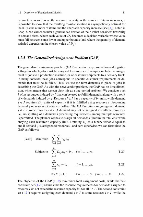
The generalized assignment problem (GAP) arises in many production and logisticssettings in which jobs must be assigned to resources. Examples include the assign-ment of jobs to a production machine, or of customer shipments to a delivery truck.In many contexts these jobs correspond to specific customer requirements or de-mands that must be fulfilled. Thus, we use the term demands in place of jobs indescribing the GAP. As with the newsvendor problem, the GAP has no time dimen-sion, which means that we can view this as a one-period problem. We consider a setI of m resources indexed by i that can be used to fulfill demands, along with a set J
of n demands indexed by j . Resource i ∈ I has a capacity of bi units, while demandj ∈ J requires Dij units of capacity if it is fulfilled using resource i. Processingdemand j on resource i costs cij dollars. The GAP requires assigning each demandj ∈ J to some resource i ∈ I . A demand may not be assigned to multiple resources,i.e., no splitting of a demand’s processing requirements among multiple resourcesis permitted. The planner wishes to assign all demands at minimum total cost whileobeying each resource’s capacity limit. Defining xij as a binary variable equal toone if demand j is assigned to resource i, and zero otherwise, we can formulate theGAP as follows:
[GAP] Minimizem∑
i=1
n∑j=1
cij xij (1.19)
Subject ton∑
j=1
Dijxij ≤ bi, i = 1, . . . ,m, (1.20)
m∑i=1
xij = 1, j = 1, . . . , n, (1.21)
xij ∈ {0,1}, i = 1, . . . ,m, j = 1, . . . , n. (1.22)
The objective of the GAP (1.19) minimizes total assignment costs, while the firstconstraint set (1.20) ensures that the resource requirements for demands assigned toresource i do not exceed the resource capacity bi , for all i ∈ I . The second constraintset (1.21) requires assigning each demand j ∈ J to some resource i ∈ I , while the

12 1 Scope of Problem Coverage and Introduction
final constraint set (1.22) ensures that each assignment variable takes a value of zeroor one. Later in Chaps. 7 and 8 we will explore a more general version of the GAPthat permits flexibility in satisfying demand requirements. For an early definition ofthe GAP, please see [3].
1.2.6 The Facility Location Problem (FLP)
The facility location problem (FLP) we next present generalizes two of the modelswe have already discussed: the ELSP and the GAP. Although the model originated incontexts requiring location decisions for physical facilities, we can view it as a moregeneric fixed-charge assignment or bipartite network flow problem. In particular, wecan view the FLP as a generalization of the GAP in which a fixed-charge is incurredwhen using any resource. Thus, if Si denotes the fixed charge for using resourcei, and yi denotes a binary variable equal to one if resource i is utilized (and zerootherwise), then we can formulate this more general version of the GAP as follows:
[FLP] Minimizem∑
i=1
Siyi +m∑
i=1
n∑j=1
cij xij (1.23)
Subject ton∑
j=1
Djxij ≤ biyi, i = 1, . . . ,m, (1.24)
m∑i=1
xij = 1, j = 1, . . . , n, (1.25)
x ∈ Ω, (1.26)
yi ∈ {0,1}, i = 1, . . . ,m. (1.27)
The objective of the FLP (1.23) minimizes the sum of resource fixed costs plus de-mand assignment costs. The first constraint set (1.24) differs from (1.20) becausethe demand is independent of the facility (hence the Dj instead of Dij ) and in theextra yi term multiplying the capacity on the right-hand side. This constraint thusonly permits assigning demands to a resource if the associated fixed cost is absorbed(and yi = 1). The third constraint set (1.26) differs from our formulation of the GAPas we now require that each variable xij is a member of some m × n dimensionalset Ω . When Ω = [0,1]m×n, then we permit splitting each demand among multi-ple resources by allowing the assignment (xij ) variables to be continuous. WhenΩ = {0,1}m×n, then this version of the problem is known as the FLP with single-sourcing requirements; strictly speaking, the FLP with single sourcing generalizesthe GAP, and the formulation of the FLP when Ω = [0,1]m×n is a relaxation of thesingle-sourcing version of the problem (note that when capacities are unlimited, thisdistinction is not necessary, as an optimal single-sourcing solution is guaranteed to

References 13
exist). The remaining constraint set (1.27) imposes binary restrictions on the newfixed-charge (yi ) variables.
Observe that in addition to generalizing the ELSP and GAP, when the assignmentconstraints (1.25) are relaxed (either by omitting them or by changing the equality toa less than or equal to relation) and m = 1 (only a single resource exists with S1 = 0),then the FLP reduces to the KP if the c1j values are permitted to be negative (and−c1j is equal to Rj ).
To see how the ELSP serves as a special case of FLP, observe that we can re-formulate the ELSP as follows. We first define xts as the percentage of demandin period s that is satisfied using procurement in period t , for all t = 1, . . . , T
and s = t, . . . , T . In terms of the ELSP formulation, we have Qt = ∑Ts=t Dsxts
and It = ∑tτ=1
∑Ts=τ Dsxτs − ∑t
τ=1 Dτ . We next define cts as the cost (procure-ment plus holding) to satisfy demand in period s using production in period t , i.e.,
cts = (Ct +∑s−1τ=t Hτ )Ds . We can then formulate the ELSP equivalently as follows:
[FELSP] MinimizeT∑
t=1
Styt +T∑
t=1
T∑s=t
ctsxts (1.28)
Subject toT∑
s=t
Dsxts ≤ Mtyt , t = 1, . . . , T , (1.29)
s∑t=1
xts = 1, s = 1, . . . , T , (1.30)
xts ≥ 0, t = 1, . . . , T , s = t, . . . , T , (1.31)
yt ∈ {0,1}, t = 1, . . . , T . (1.32)
The FELSP formulation is equivalent to the ELSP formulation, and is a special caseof the FLP in which a demand may be assigned to only a subset of the resources, andresource capacities are effectively unlimited (in this case, the resources correspondto period orders or production setups). In addition, the FELSP formulation implicitlyassumes that the size of each demand s is independent of the resource to which itis assigned (hence the single s index for Ds ). By replacing each Mt with a finitevalue bt , we obtain the capacitated version of the ELSP. Note that the uncapacitatedversion of the FLP is obtained by replacing each bi in (1.24) with a big-Mi value(e.g., Mi = ∑n
j=1 Dij for each i = 1, . . . ,m). The uncapacitated version of the FLP(and, therefore, the FELSP formulation) has the property that an optimal solutionexists in which the xij variables are binary, i.e., a single-sourcing solution is optimaleven though it is not explicitly required.
References
1. Aggarwal A, Park J (1993) Improved Algorithms for Economic Lot Size Problems. OperationsResearch 41(3):549–571

14 1 Scope of Problem Coverage and Introduction
2. Anton H (1988) Calculus. Wiley, New York3. De Maio A, Roveda C (1971) An All Zero-One Algorithm for a Certain Class of Transporta-
tion Problems. Operations Research 19(6):1406–14184. Federgruen A, Tzur M (1991) A Simple Forward Algorithm to Solve General Dynamic Lot
Sizing Models with n Periods in O(n logn) or O(n) Time. Management Science 37(8):909–925
5. Frieze A, Clarke M (1984) Approximation Algorithms for the m-Dimensional 0–1 KnapsackProblem: Worst-Case and Probabilistic Analyses. European Journal of Operational Research15(1):100–109
6. Garey M, Johnson D (1979) Computers and Intractability. W.H. Freeman and Company, NewYork
7. Hadley G, Whitin T (1961) An Optimal Final Inventory Model. Management Science7(2):179–183
8. Harris F (1913) How Many Parts to Make at Once. Factory Magazine Management 10:135–136, 152
9. Silver E, Pyke D, Peterson R (1998) Inventory Management and Production Planning andScheduling, 3rd edn. Wiley, New York
10. Wagelmans A, van Hoesel S, Kolen A (1992) Economic Lot Sizing: An O(n logn) AlgorithmThat Runs in Linear Time in the Wagner-Whitin Case. Operations Research 40(S1):S145–S156
11. Wagner H, Whitin T (1958) Dynamic Version of the Economic Lot Size Model. ManagementScience 5(1):89–96

Chapter 2Production and Inventory Planning Modelswith Demand Shaping
Abstract This chapter considers the state of prior literature on operations modelsthat account for demand flexibility. In particular, we focus on generalizations ofthe models discussed in Chap. 1 that treat demands as decision variables. Thesegeneralizations typically involve pricing models, and they provide a foundation forthe models we will study in subsequent chapters.
2.1 EOQ Models with Pricing
Whitin [37] provided a seminal paper on inventory control and pricing under theEOQ model assumptions (this paper also considers a single-period stochastic prob-lem, which we discuss in the following section). This model generalizes cost equa-tion (1.4) to account for price-dependent demand and subsequently maximizes profitper unit time instead of cost. In order to do this, a linear price–demand function isassumed that takes the form
D = β − αp, (2.1)
where α and β are scalars (which are typically assumed to be positive) and p denotesprice. Using this demand function (2.1) along with cost Eq. (1.4), we can write theaverage profit per unit time as a function of p, denoted as Π(p), as
Π(p) = (p − C)(β − αp) − √2S(β − αp)H. (2.2)
Letting Q∗(p) = √2S(β − αp)/H , Arcelus and Srinivasan [3] provide the follow-
ing form of the stationary-point solution for the optimal price1:
p∗ = 1
2
[β
α+ C + S
Q∗(p∗)
], (2.3)
1One can verify that the second derivative of Π(p) with respect to p is strictly increasing in p;thus the profit function Π(p) is either convex in p for all p ≥ 0, in which case an optimal extremepoint solution exists (i.e., either p∗ = 0 or p∗ = β/α), or Π(p) is concave on some interval [0, p]and convex for p ≥ p. In the latter case, either an extreme solution or the stationary-point solution(2.3) is optimal (assuming such a stationary point exists).
J. Geunes, Demand Flexibility in Supply Chain Planning,SpringerBriefs in Optimization,DOI 10.1007/978-1-4419-9347-2_2, © Joseph Geunes 2012
15

16 2 Production and Inventory Planning Models with Demand Shaping
where
Q∗(p∗) =√
2S(β − αp∗)H
. (2.4)
This generalized version of the EOQ model permits selecting the optimal demandlevel when demand is price-dependent (for simplicity, we have considered a lin-ear price–demand function, although more complex functions have been explored).Numerous additional generalizations of this basic model have been addressed in theliterature, including problems with more general demand functions ([23, 25, 31]),quantity discounts ([1, 8, 9]), and investment and storage constraints ([7, 24]).
2.2 The Newsvendor Problem with Pricing and Demand Shaping
As noted in the previous section, Whitin [37] first considered a single period inven-tory problem with pricing under demand uncertainty. This problem used a marginalanalysis with a unit profit for items sold and a unit loss associated with excess in-ventory remaining after demand is realized. Assuming that expected demand is alinear function of the profit margin and that demand is uniformly distributed be-tween zero and twice the expected demand, Whitin [37] derived an expression forthe optimal profit margin. The demand model used by Whitin [37] is effectively amultiplicative model, as both the expected value and the variance of the demand dis-tribution depend on price. This is in contrast with the additive model, where demandis expressed as a deterministic function of price plus a random error term, which isindependent of price. That is, letting D(p, ε) denote the demand function, where ε
is a random variable, then in an additive model, D(p, ε) = y(p) + ε, where y(p)
is a deterministic function of price and ε is a random variable with mean μ andvariance σ 2. Under a multiplicative model, we have D(p, ε) = y(p)ε. The form ofthe demand model assumed fundamentally affects both the quantitative and qualita-tive results of the model. We will first briefly illustrate the application of a simpleadditive demand model and then discuss more general work that subsumes both theadditive and multiplicative cases.
We initially consider the basic newsvendor problem under normal demand dis-cussed in Chap. 1. Consider a generalized version of the expected profit equation(1.10) in which the expected demand μD is price dependent. In particular, assumethat μD = α − βp. In this case, Eq. (1.10) becomes
Πn
(Q∗,p
) = (p − C)(α − βp) − K(z∗)σD. (2.5)
This profit equation is concave in p with stationary-point solution (and thereforeoptimal solution) p∗
a = (1/2)(C + (α/β)), where the subscript a corresponds tothe additive case. Observe that for this additive demand model, the optimal pricedepends only on the profit margin (p−C) and the expected demand, i.e., the optimalprice is the same as that for the zero-variance (risk-free) case. The same is not truein a multiplicative model.

2.2 The Newsvendor Problem with Pricing and Demand Shaping 17
To illustrate this, suppose that, in addition, σD is a linear function of price, i.e.,σD = (α − βp)σ . This is equivalent to a multiplicative model in which y(p) =(α − βp) and ε is normally distributed with expected value one and variance σ 2.In this special case, the expected profit equation remains concave in p, and thestationary-point optimal solution becomes p∗
m = (1/2)(C + (α/β) + K(z∗)σ ) =p∗
a + (K(z∗)σ/2), where the subscript m corresponds to the multiplicative case.Thus, the price in the multiplicative case equals the risk-free (additive) price plus apremium for the way in which price affects uncertainty.
Petruzzi and Dada [29] provide an excellent, general, and detailed analysis ofthe newsvendor problem with pricing. We next summarize their main results, whichunify the treatment of the additive and multiplicative cases. These results build onthe foundations provided in [13, 21, 28, 37, 38], and [39]. Petruzzi and Dada [29]consider an expected profit function of the form
Π(Q,p) = (p − C)E[Sales(ζ,p)
] − (C + H)E[Leftovers(ζ,p)
]
− BE[Shortages(ζ,p)
], (2.6)
where a one-to-one correspondence exists between the variable ζ and the orderquantity Q at any price. The relationship between Q and ζ depends on the formof the demand function. In the additive case, ζ is defined using ζ = Q − y(p). Inthe multiplicative case, ζ is defined using ζ = Q/y(p).
Petruzzi and Dada [29] show that, for both the additive and multiplicative demandcases, ζ can be written as
ζ = μ + SFσ, (2.7)
where SF is defined in [32] as the safety factor, which is the number of standarddeviations by which the order quantity differs from the expected value of demand,i.e.,
SF = Q − E[D(p, ε)]SD[D(p, ε)] , (2.8)
where SD[D(p, ε)] is the standard deviation of D(p, ε). They then define the baseprice, pB(ζ ) as the price that maximizes the expected contribution to profit fromsales, i.e., the price that maximizes (p − C)E[Sales(ζ,p)] (note that pB(ζ ) maxi-mizes the risk-free profit, i.e., expected profit when variance equals zero). Their firstmain result shows that for both the additive and multiplicative cases, for a given ζ ,pB(ζ ) is determined by the unique value of p satisfying
p = C − E[Sales(ζ,p)]∂E[Sales(ζ,p)]/∂p . (2.9)
The second main result states that the optimal price in both the multiplicative andadditive cases is bounded from below by pB(ζ ) for any given ζ . This implies that forboth cases we can view the optimal price as the optimal base price plus a premium.In the additive case this premium equals zero because, for any given ζ , the expectedleftover and shortage costs are independent of price. In the multiplicative case, the

18 2 Production and Inventory Planning Models with Demand Shaping
premium depends on the impact the price has on expected holding and shortagecosts. Petruzzi and Dada [32] provide functional forms for the optimal price in boththe multiplicative and additive cases, as well as methods to determine the optimalcorresponding order quantity.
In addition to shaping demand through pricing, a few papers have considereddifferent dimensions of demand flexibility in a stochastic demand setting. Petruzziand Monahan [30] consider a fashion goods context with a primary and secondarymarket, where the decision maker must determine the optimal time at which to movea good from the primary to the secondary market. Carr and Duenyas [5] considera production system with two classes of demand, each of which has a Poisson dis-tributed arrival rate. Type 1 demands are called make-to-stock demands, and Type 2demands are called make-to-order demands. Type 1 demands result in a shortagecost if a demand occurs and stock is depleted, while Type 2 demands may be ac-cepted or rejected, although those accepted demands are made-to-order. This workprovides an optimal production and order acceptance policy for this problem class.Carr and Lovejoy [6] consider a single-period newsvendor-type problem in whicha number of prioritized demand portfolios are available, and a single resource withrandom capacity may be used to satisfy demands. The decision maker must deter-mine the amount of demand to select within each portfolio in order to maximizeexpected profit.
2.3 Lot Sizing with Pricing
The earliest work on integrating pricing in the ELSP appears to be that of Thomas[33]. His work generalized the ELSP to incorporate the dependence of demand ineach period on price. In this model, price may vary from period to period, and de-mand in period t depends on the price in period t , pt , according to the functionDt(pt ). This generalization of the ELSP can be formulated as follows:
[ELSP′] MaximizeT∑
t=1
{ptDt(pt ) − Styt − CtQt − HtIt
}(2.10)
Subject to It = Qt + It−1 − Dt(pt ), t = 1, . . . , T , (2.11)
Qt ≤ Mtyt , t = 1, . . . , T , (2.12)
Qt, It ,pt ≥ 0, t = 1, . . . , T , (2.13)
yt ∈ {0,1}, t = 1, . . . , T . (2.14)
The solution approach relies on the fact that for any given price vector, the problemreduces to the ELSP, and the zero-inventory-ordering (ZIO) property continues tohold. This implies that the shortest path solution approach discussed in Chap. 1 maystill be applied in principle, although it becomes an acyclic longest path problemin which arcs are assigned profits instead of costs. If, for example, production in

2.3 Lot Sizing with Pricing 19
period t satisfies demand in periods t through s, then the profit on the arc from nodet to node s + 1 is obtained by solving the following pricing subproblem PSP where,with a slight abuse of notation, Ht,τ = ∑τ−1
u=t Hu:
[PSP] Maximizes∑
τ=t
{(pτ − Ct − Ht,τ )Dτ (pτ )
}. (2.15)
The PSP above decomposes by period, and its difficulty depends on the specificationof the demand functions Dt(pt ). If the optimal solution value to the PSP is less thanor equal to the fixed order cost in period t , St , then the maximum arc (t, s +1) profitequals zero; otherwise the arc profit equals the optimal objective function value lessSt . Thomas [33] illustrates the case in which Dt(pt ) is linear in pt for t = 1, . . . , T ,which implies that the PSP is easily solved using first order conditions.
Kunreuther and Schrage [22] subsequently considered the problem when pricemust be time-invariant, which is equivalent to adding the constraints pt = pt+1 fort = 1, . . . , T − 1, to the ELSP′ formulation. This restriction of the problem leadsto a very different algorithm for solving the problem, because the problem can nolonger be solved by decomposition into smaller time horizons, and the shortest pathsolution we described is no longer possible. However, as we know that for any givenprice p = p1 = p2 = · · · = pT , the problem again reduces to the ELSP. Thus, weknow that an optimal solution exists that satisfies the ZIO property and that maybe completely characterized by the sequence of order periods. That is, if we knowthere are ρ order periods t1, t2, . . . , tρ , then the corresponding ZIO solution produces∑tj+1−1
τ=tjDτ (p) in period tj for j = 1, . . . , ρ. We will refer to a specific set of order
periods t1, t2, . . . , tρ as an order plan. Kunreuther and Schrage [22] assume thatdemand in any period t is a linear function of a price effect function d(p), which istime invariant. That is, Dt(p) = αt + βtd(p) for t = 1, . . . , T , where αt and βt arenonnegative constants for each period t . For the special case in which d(p) = −p,we have the familiar linear price–demand function Dt(p) = αt − βtp.
Observe that, given any price p, a vector of demands [D(p)] =[D1(p), . . . ,DT (p)] results. The revenue associated with this demand vector equals∑T
t=1 pDt(p). The cost associated with this vector of demands depends on the or-der plan utilized (we confine ourselves to the order plans defined in the previousparagraph, since we know that an optimal solution exists from among these solu-tions). As shown in [22], the cost of any order plan can be expressed as a linearfunction of the price effect d(p). Assuming d(p) = −p, or a linear price–demandrelationship in each period, this implies that the minimum cost as a function of p
is a piecewise linear and concave function of p, where each linear segment cor-responds to a specific order plan. If we can specify this piecewise linear function,or envelope, then it is possible to evaluate the maximum profit associated with ev-ery candidate order plan contained in an optimal solution. In this case, for eachsegment of the piecewise linear function, we can compute the optimal price forthe given order plan. Specifying this piecewise linear function is not trivial, how-ever.

20 2 Production and Inventory Planning Models with Demand Shaping
Kunreuther and Schrage [22] suggest a heuristic approach that assumes the op-timal price must fall on some interval [pL,pU ]. We next briefly sketch the waythis heuristic works. First, recall that for any fixed price, the problem reduces toan ELSP. Thus, we can initially solve the problem at the price pL, which requiressolving an instance of the ELSP. This solution provides an optimal order plan at theprice pL. The cost of this order plan is linear in price, and the associated line mustform a segment of the piecewise linear concave envelope. Given this order plan,we next determine the price that maximizes profit when restricting ourselves to thisparticular order plan. If this price differs from pL, then we can solve the ELSP cor-responding to this new price. If the optimal order plan differs from the previous one,then we have identified an additional segment of the piecewise linear concave enve-lope. We continue this procedure iteratively, until the price and order plan converge.Call the resulting price after convergence p∗
L. We then repeat this process using thestarting price pU , and converging to the price p∗
U . As shown in [22], the optimalprice, p∗, satisfies p∗
L ≤ p∗ ≤ p∗U .
Gilbert [15] considered a special case of this model in which costs are time-invariant and Dt(p) = βtd(p). For this case, he showed that the piecewise linearconcave envelope has at most O(T ) segments, and that these segments can be iden-tified in polynomial time. Van den Heuvel and Wagelmans [35] then provided analgorithm that permits identifying the entire piecewise linear concave envelope forthe general case defined in [22]. Beginning with the solutions p∗
L and p∗U , they show
how to identify whether an unidentified segment of the piecewise linear concave en-velope exists by solving the problem at the intersection of the lines corresponding tothe optimal order plans at the prices p∗
L and p∗U . If a new line segment is identified,
and its optimal price is also identified, this permits eliminating part of the intervalof uncertainty2 between p∗
L and p∗U . This can then be repeated for any remaining
intervals of uncertainty. Because the number of order plans is finite, the procedureis finite and must converge to an optimal price.
Gilbert [16] considered a multiple product lot sizing problem with shared buttime-invariant production capacities and a time-invariant price for each good. Dengand Yano [10] and Geunes, Merzifonluoglu, and Romeijn [14] subsequently con-sidered the integrated pricing and lot sizing problem with production capacities.Merzifonluoglu, Geunes, and Romeijn [27] considered a class of aggregate planningproblems in which capacities, prices, and subcontracting levels served as decisionvariables.
2.4 Knapsack Problems with Nonlinear Objectives
This section describes a class of continuous knapsack problems in which a set J ofn demands exists, as in our discussion of knapsack problems in Chap. 1. In this class
2We define an interval of uncertainty as an interval which is known to contain the optimal price,although the precise value of the optimal price remains unknown.

2.4 Knapsack Problems with Nonlinear Objectives 21
of knapsack problems, however, the variable xj no longer corresponds to a binaryvariable that determines whether or not demand j is selected. Instead, xj denotesa variable corresponding to the percentage of some maximum level, Dj , at whichdemand j may be satisfied. For example, Dj might correspond to the maximumlevel of sales effort that may be applied in a market j or the maximum amount ofadvertising expenditures that may be dedicated to product j . In each of these cases,the activity level consumes part of a finite resource with capacity b (in the formercase this resource may be a salesperson’s time in a period, while in the latter thisresource may be a limited budget).
Associated with demand j is a revenue function Rj (xj ), which depends on theactivity level for demand j . We can formulate this nonlinear revenue maximizingknapsack problem as follows:
[NLKP] Maximizen∑
j=1
Rj (xj ) (2.16)
Subject ton∑
j=1
Djxj ≤ b, (2.17)
0 ≤ xj ≤ 1, j = 1, . . . , n. (2.18)
Clearly if each Rj (·) function is linear in xj , then NLKP corresponds to the con-tinuous relaxation of the knapsack problem KP defined in Chap. 1. If each Rj (·)function is convex in xj , then an extreme point optimal solution also exists (as inthe relaxation of KP). It is straightforward to show that extreme point solutions forNLKP contain at most one xj variable that takes a value strictly between zero andone (moreover, for such extreme solutions, the resource capacity constraint (2.17)is tight). Using this fact, [4] provides a pseudopolynomial time algorithm underconvex revenue functions that runs in O(Un2b) time in the worst case, where U
denotes the maximum value of Dj over all j ∈ J (assuming that b and all Dj areinteger). When all revenue functions are concave, the NLKP is a convex programand can therefore be solved using standard nonlinear optimization solvers. Moregeneral so-called S-curve return functions are considered in [2] and [17]. Thesefunctions arise in numerous marketing contexts such as advertising, where smalllevels of investment provide increasing returns to scale, and larger investment levelslead to decreasing returns to scale. Such S-curve functions are convex from zero toan inflection point, and then are concave thereafter. Analysis of the special structureof these revenue functions leads to pseudopolynomial time solution methods (see[2, 17]).
Additional classes of generalized knapsack problems with demand flexibility willarise in our study of decomposition methods for assignment and location models inChap. 8. Moreover, in our analysis of EOQ models in Chap. 3 and in our discussionof newsvendor models in Chap. 4, several interesting nonlinear and nonseparableknapsack problems will arise.

22 2 Production and Inventory Planning Models with Demand Shaping
2.5 Location and Assignment Problems with Flexible Demand
Location theory has been well studied in the economics and operations researchliterature under a number of assumptions. Much of the literature on location the-ory with price effects applies game-theoretic analysis in competitive settings. Thisbody of literature simultaneously considers the objectives of multiple competing or-ganizations, each of which wishes to maximize its profit based on its location andmarket-supply decisions. A discussion of the models and approaches for this classof problems may be found in [11] and [34]. The models we consider, and whichare most relevant to the work considered throughout this book, are more appropriatefor a single firm who is a monopolist, and thus wishes to make location decisionsbased on response to a price–demand curve for its product (and independent of otherfirms’ decisions).
Wagner and Falkson [36] provided perhaps the earliest model for a facility loca-tion problem facing a single monopolistic producer of a good with price-sensitivedemand. This model considered the location of public facilities under the maximiza-tion of social welfare and several different assumptions on the level of service thatmust be provided to customers. Hansen and Thisse [19] then provided a model fora private firm seeking to simultaneously determine price and location decisions inorder to maximize profit when demand is price-dependent. Erlenkotter [12] general-ized their approach to account for the profit maximization objectives of private andpublic firms within a single model. He provided a heuristic algorithmic approachbased on Lagrangian relaxation and explicitly considered situations in which therevenue in a customer market is a quadratic function of price. The models we havediscussed thus far permit charging different prices to individual markets, where theoptimal price in a market depends on which facility serves the market at optimality.Hansen, Thisse, and Hanjoul [20] modeled the problem when the delivered pricemust be the same for all markets. Hanjoul et al. [18] later provided models thatallowed different methods of consistent pricing among customers (that is, they con-sidered the case in which the delivered price is the same for all customer markets, aswell as the case in which all customers pay the same mill price, i.e., the price beforebearing transportation costs from the supply point).
Although work on the generalized assignment problem (GAP) with pricing isquite limited, a rich set of models exists in the marketing literature for determin-ing the optimal amount of limited salesforce effort to exert in different territories(see, e.g., [26, 40]). In these models, a salesperson’s time corresponds to a lim-ited resource, and sales territories must be assigned to sales personnel. Given anassignment of territories to a salesperson, the time the salesperson spends in eachterritory must also be determined, where the sales response (or revenue function, asin the NLKP) in a territory is a nonlinear function of the time spent in the territory(or the effort exerted). Thus, the sales level within each territory (i.e., the demand)effectively serves as a decision variable that is determined via the level of saleseffort.

References 23
References
1. Abad P (1988) Determining Optimal Selling Price and Lot Size When the Supplier OffersAll-Unit Quantity Discounts. Decision Sciences 19(3):622–634
2. Agralı S, Geunes J (2009) Solving Knapsack Problems with S-Curve Return Functions. Euro-pean Journal of Operational Research 193:605–615
3. Arcelus F, Srinivasan G (1998) Ordering Policies under One Time Only Discount and PriceSensitive Demand. IIE Transactions 30:1057–1064
4. Burke G, Geunes J, Romeijn H, Vakharia A (2008) Allocating Procurement to CapacitatedCuppliers with Concave Quantity Discounts. Operations Research Letters 36:103–109
5. Carr S, Duenyas I (2000) Optimal Admission Control and Sequencing in a Make-to-Stock/Make-to- Order Production System. Operations Research 48(5):709–720
6. Carr S, Lovejoy W (2000) The Inverse Newsvendor Problem: Choosing an Optimal DemandPortfolio for Capacitated Resources. Management Science 46(7):912–927
7. Cheng T (1990) An EOQ Model with Pricing Consideration. Computers and IE 18(4):529–534
8. Dada M, Srikanth K (1987) Pricing Policies for Quantity Discounts. Management Science33(10):1247–1252
9. Das C (1984) A Unified Approach to the Price-Break Economic Order Quantity (EOQ) Prob-lem. Decision Sciences 15(3):350–358
10. Deng S, Yano C (2006) Joint Production and Pricing Decisions with Setup Costs and CapacityConstraints. Management Science 52(5):741–756
11. Eiselt H, Laporte G, Thisse J (1993) Competitive Location Models: A Framework and Bibli-ography. Transportation Science 27(1):44–54
12. Erlenkotter D (1977) Facility Location with Price-Sensitive Demands: Private, Public, andQuasi-Public. Management Science 24(4):378–386
13. Ernst R (1970) A Linear Inventory Model of a Monopolistic Firm. PhD Dissertation, Depart-ment of Economics, University of California, Berkeley, CA
14. Geunes J, Merzifonluoglu Y, Romeijn H (2009) Capacitated Procurement Planning withPrice-Sensitive Demand and General Concave Revenue Functions. European Journal of Op-erational Research 194:390–405
15. Gilbert S (1999) Coordination of Pricing and Multiple-Period Production for Constant PricedGoods. European Journal of Operational Research 114:330–337
16. Gilbert S (2000) Coordination of Pricing and Multiple-Period Production Across MultipleConstant Priced Goods. Management Science 46:1602–1616
17. Ginsberg W (1974) The Multiplant Firm with Increasing Returns to Scale. Journal of Eco-nomic Theory 9:283–292
18. Hanjoul P, Hansen P, Peeters D, Thisse J (1990) Uncapacitated Plant Location under Alterna-tive Spatial Price Policies. Management Science 36(1):41–57
19. Hansen P, Thisse J (1977) Multiplant Location for Profit Maximization. Environment andPlanning A 9:63–73
20. Hansen P, Thisse J, Hanjoul P (1980) Simple Plant Location under Uniform Delivered Pricing.European Journal of Operational Research 6:94–103
21. Karlin S, Carr C (1962) Prices and Optimal Inventory Policy. In Studies in Applied Probabil-ity and Management Science (Arrow K, Karlin S, Scarf H (eds.)) Stanford University Press,Stanford, CA, 159–172
22. Kunreuther H, Schrage L (1973) Joint Pricing and Inventory Decisions for Constant PricedItems. Management Science 19(7):732–738
23. Ladany S, Sternlieb A (1974) The Interaction of Economic Ordering Quantities and MarketingPolicies. AIIE Transactions 6(1):35–40
24. Lee W (1994) Optimal Order Quantities and Prices with Storage Space and Inventory Invest-ment Limitations. Computers and IE 26(3):481–488
25. Lee W, Kim D (1993) Optimal and Heuristic Decision Strategies for Integrated Productionand Marketing Planning. Decision Sciences 24(6):1203–1213

24 2 Production and Inventory Planning Models with Demand Shaping
26. Lodish L (1971) CALLPLAN: An Interactive Salesman’s Call Planning System. ManagementScience 18:4 Part II:25–40
27. Merzifonluoglu Y, Geunes J, Romeijn H (2007) Integrated Capacity, Demand, and ProductionPlanning with Subcontracting and Overtime Options. Naval Research Logistics 54(4):433–447
28. Mills E (1959) Uncertainty and Price Theory. The Quarterly Journal of Economics 73:116–130
29. Petruzzi N, Dada M (1999) Pricing and the Newsvendor Problem: A Review with Extensions.Operations Research 47(2):183–194
30. Petruzzi N, Monahan G (2003) Managing Fashion Goods Inventories: Dynamic Recourse forRetailers with Outlet Stores. IIE Transactions 35(11):1033–1047
31. Rosenberg D (1991) Optimal Price-Inventory Decisions-Profit vs. ROII. IIE Transactions23(1):17–22
32. Silver E, Pyke D, Peterson R (1998) Inventory Management and Production Planning andScheduling, 3rd edn. Wiley, New York
33. Thomas J (1970) Price-Production Decisions with Deterministic Demand. Management Sci-ence 16(11):747–750
34. Tobin R, Miller T, Friesz T (1995) Incorporating Competitors’ Reactions in Facility LocationDecisions: A Market Equilibrium Approach. Location Science 3(4):239–253
35. Van den Heuvel W, Wagelmans A (2006) A Polynomial Time Algorithm for a DeterministicJoint Pricing and Inventory Model. European Journal of Operational Research 170:463–480
36. Wagner J, Falskon L (1975) The Optimal Nodal Location of Public Facilities with Price-Sensitive Demand. Geographical Analysis 7(1):69–83
37. Whitin T (1955) Inventory Control and Price Theory. Management Science 2(1):61–6838. Young L (1978) Price, Inventory and the Structure of Uncertain Demand. New Zealand Oper-
ations Research 6:157–17739. Zabel E (1970) Monopoly and Uncertainty. The Review of Economic Studies 37:205–21940. Zoltners A (1976) Integer Programming Models for Sales Territory Alignment to Maximize
Profit. Journal of Marketing Research 13(4):426–430

Part IIProduction Planning with Demand
Flexibility

Chapter 3EOQ-Type Models with Demand Selection
Abstract This chapter discusses a generalized version of the economic order quan-tity (EOQ). In particular, we consider a situation in which a single inventory stagemust select from among a set of demand streams, those which it will satisfy. Eachdemand stream carries with it a constant demand rate as well as a constant revenuerate. We consider several problem variants within this class, including problemswith lot size and demand rate constraints.
3.1 Unconstrained EOQ Problems with Market Choice
The problems and results discussed in this chapter are based on work previouslypublished in [2], which contains detailed results on this problem class. We will firstconsider a generalization of the standard EOQ model in Sect. 3.1.1 (with an infiniteproduction rate), and then extend the results to the case with a finite production ratein Sect. 3.1.2.
3.1.1 Standard EOQ with Market Choice
We consider a set J of n markets, indexed by j , where market j demand occurs ata constant rate of Dj units per unit time. In the analysis of the basic EOQ problemin Chap. 1, a single “market” existed and the supplier was required to serve all ofthis market’s demand. In the EOQ problem with market choice (EOQMC), the sup-plier can choose whether or not to serve the demand in each market. If the supplierchooses to satisfy demand in market j , it must satisfy all of the market’s demandwithout any shortages. We therefore define a set of binary variables, where xj equalsone if the supplier meets all demand in market j , and zero otherwise. Thus, giventhe values of these variables, the single stage faces a demand rate equal to
∑
j∈J
Djxj . (3.1)
J. Geunes, Demand Flexibility in Supply Chain Planning,SpringerBriefs in Optimization,DOI 10.1007/978-1-4419-9347-2_3, © Joseph Geunes 2012
27

28 3 EOQ-Type Models with Demand Selection
Under this demand rate, the optimal batch order quantity equals
Q∗(x) =√
2S∑
j∈J Djxj
H, (3.2)
where x denotes an n-dimensional binary vector of xj values. If rj denotes the netrevenue per unit of demand sold in market j (in excess of the variable cost C), thenif the supplier satisfies demand in market j , the average revenue per unit time frommarket j equals Rj = rjDj . Thus, the average total revenue per unit time can beexpressed as
∑
j∈J
Rjxj . (3.3)
Referring back to Eq. (1.4), we can express average profit per unit time from marketselection decisions, Π(x), as
Π(x) =∑
j∈J
Rjxj −√
2SH∑
j∈JDjxj . (3.4)
The supplier wishes to maximize Π(x) over all x vectors in Bn, the space contain-ing all n-dimensional binary vectors. The following result, from [3], will be utilizedin solving this problem as well as additional problems in this chapter and the next.
Property 3.1 Consider the problem maxx∈Bn{∑j∈J Rjxj −√∑
j∈J κj xj }, with
κj > 0 for all j = 1, . . . , n. Assuming demands are sorted in nonincreasing order ofthe ratio Rj/κj , if an optimal solution exists with xk = 1 for some index k, then anoptimal solution exists with xk−1 = 1.
Proof Because the objective function is convex in x, this implies that an extremepoint solution exists for solving the relaxation in which the requirement x ∈ Bn
is replaced with 0 ≤ xj ≤ 1 for all j = 1, . . . , n. Observe that the objective is dif-ferentiable for x ≥ 0 everywhere except at x = 0. Thus, the Karush–Kuhn–Tucker(KKT) optimality conditions are necessary for an optimal solution (see [1]), ex-cept possibly at the point x = 0, where average profit per unit time equals zero. Wecan therefore consider all KKT points, along with the solution x = 0 in searchingfor an optimal solution. Let α0
j (α1j ) denote the KKT multiplier associated with the
constraint −xj ≤ 0 (xj ≤ 1). The associated KKT conditions can be written as
Rj − κj
2√∑
j∈J κj xj
− α1j + α0
j = 0, ∀j ∈ J, (3.5)
α0xj = 0, ∀j ∈ J, (3.6)
α1(1 − xj ) = 0, ∀j ∈ J, (3.7)
0 ≤ xj ≤ 1, ∀j ∈ J, (3.8)
α0j , α
1j ≥ 0, ∀j ∈ J. (3.9)
3.1 Unconstrained EOQ Problems with Market Choice 29
Because all extreme point solutions are binary, we only need to consider such solu-tions. Thus, each xj equals zero or one. If xj = 1, then we must have α0
j = 0, whichimplies
Rj
κj
≥ 1
2√∑
j∈J κj xj
, (3.10)
and if xj = 0, then we must have α1j = 0, which implies
Rj
κj
≤ 1
2√∑
j∈J κj xj
. (3.11)
Because the right-hand side of (3.11) is the same as that of (3.10), and this value isfixed at any point, this implies a strict ordering of Rj/κj values. (We assume theseratios are unique. If two or more demands exist with an identical ratio, we combinethem into a single demand.) If we index demands based on this ratio, and if (3.10)holds for demand k, it must also hold for demand k − 1. Therefore, if a KKT pointexists such that xk = 1, then a KKT point also exists with xk−1 = 1. The necessityof the KKT conditions implies the result.1 �
This property implies that we can index demands in nonincreasing order ofRj/Dj = rj , or unit revenue values, and an optimal solution will be of the formxj = 1 for j = 1, . . . , k and xj = 0 for j = k + 1, . . . , n, for some k between oneand n. There are n solutions of this form, and we can sort demands and compute theaverage profit per unit time for each solution of this form in O(n logn) time. If thesolution with the maximum average profit per unit time among these n solution haspositive average annual profit, then this solution is optimal; otherwise an optimalsolution sets xj = 0 for all j ∈ J (and Q = 0).
3.1.2 The EPQ Problem with Market Choice
The standard EOQ model discussed in the previous section is sometimes referred toas having an infinite production rate, which is equivalent to the special case in whichthe delivery lead time equals zero. When the rate at which inventory is accumulatedby the supplier is finite, the EOQ model must be generalized to account for this.Suppose that the supplier may only add to its inventory at a finite rate of P units perunit time. We will assume that this rate exceeds the maximum market demand rate(otherwise, accommodating this market without shortages would not be possible).Accounting for the effects of a finite production rate in the standard EOQ problem
1Note that this result can be shown by contradiction and using an interchange argument. That is,we suppose we have an optimal solution in which the property does not hold, and demonstrate thateither a solution exists with the same objective function value satisfying the property, or that theinitial solution is not optimal, a contradiction.

30 3 EOQ-Type Models with Demand Selection
without market choice results in only a slight modification, which is often viewed asan adjustment to the holding cost by multiplying by a constant factor. The resultingmodel is often referred to as the economic production quantity (EPQ). Accountingfor a finite production rate in the EOQ with market choice is a bit more involved,but leads to a similar result.
Under a finite production rate P , the average fixed order and holding costs perunit time for the standard EPQ model with demand rate D at the optimal orderquantity may be written as
√
2SDH
(1 − D
P
). (3.12)
Using (3.12), along with market choice decision variables, the average profitfunction per unit time for the EPQ with market choice (EPQMC) problem is writtenas
ΠP (x) =∑
j∈J
Rjxj −√√√√2SH
(∑
j∈J
Djxj
)(1 −
∑j∈J Djxj
P
). (3.13)
We can show that ΠP (x) is convex in x (see [2]), and, as a result, a binary optimalsolution exists when maximizing this function over [0,1]n, i.e., we can solve thecontinuous relaxation and obtain a binary optimal solution. As is shown in [2], thealgorithm used to solve the EOQMC can be used to find an optimal solution forthe EPQMC problem as well. We still index items in nonincreasing order of unitrevenue (rj ) values and evaluate all solutions of the form xj = 1 for j = 1, . . . , k
and xj = 0 for j = k + 1, . . . , n, for some k between one and n. The only differencelies in the evaluation of the average profit per unit time for each solution vector,which uses (3.13) instead of (3.4).
3.2 EOQMC Problems with Constraints
Practical production and inventory planning problems must often incorporate prac-tical constraints due to space, budget, or technological limits. We next consider theimplications of certain types of constraints on the problems discussed in the previ-ous section. These problems lead to interesting classes of knapsack problems withnonlinear objectives. We will first consider limits on the volume of demand that maybe satisfied per unit time, followed by batch size constraints.
3.2.1 Demand Rate Constraints
Under a limit on the amount of demand that may be satisfied per unit time, we havea constraint of the form ∑
j∈J
Djxj ≤ b, (3.14)

3.2 EOQMC Problems with Constraints 31
where b is the maximum demand rate that may be handled. While the nonlinearknapsack problem that results from maximizing either (3.4) or (3.13) over all x ∈{Bn ∩ (3.14)} is in general difficult (the recognition version in either case is N P-Complete), we can solve the continuous relaxations reasonably easily, as shownin [2].
For the EOQMC with the demand rate constraint, for example, an optimal so-lution to the continuous relaxation will exist at an extreme point, where extremepoints correspond to either binary vectors that are feasible for (3.14), or solutions inwhich (3.14) is tight and at most one xj variable is strictly between zero and one.The binary solutions generated in the algorithm for solving the unconstrained EO-QMC that are feasible for (3.14) dominate all other binary vectors that are feasiblefor the constraint. Thus, we need to consider these solutions along with an optimalsolution when (3.14) is tight in order to solve the continuous relaxation of the con-strained problem. Fortunately, when (3.14) is tight, the square root terms in (3.4)and (3.13) become fixed constants. Thus, when the constraint is tight, the problembecomes a simple continuous linear knapsack problem, which is solved by insert-ing items into the knapsack in nonincreasing order of rj values until the capacityis exhausted. Clearly this solution contains at most one fractional xj , and a solu-tion that is feasible for the binary restrictions can be obtained by simply setting thevalue of this fractional variable to zero. This rounding down heuristic is shown to beasymptotically optimal in the number of items in [2], under mild assumptions on thedistributions of parameter values and the behavior of the capacity (and productionrate, for the EPQMC) as n → ∞. Because the continuous relaxation is relativelytight (and it has an optimal solution with at most one fractional variable), solutionvia customized branch-and-bound is generally quite effective.
3.2.2 Batch Size Constraints
In some contexts, a limit may exist on the maximum amount that may be producedor delivered in response to an order (due to, e.g., space limits, transportation capacitylimits, or production technology restrictions). In this case, the associated constraintmay be written very simply as
Q ≤ b. (3.15)
We illustrate the analysis of the problem under constraint (3.15) for the EOQMCcase; for details on the EPQMC case, please see [2]. Recall that the unconstrainedoptimal order quantity is given in Eq. (3.2). However, given any binary vector x, itis possible to employ a batch size Q that is feasible for constraint (3.15), but doesnot take the form of an EOQ solution as in (3.2). We therefore consider two solutiontypes. The first type of solution uses batches from the EOQ formula that are alsofeasible for (3.15). For these solutions, the batch size constraint may be written as
∑
j∈J
Djxj ≤ b2H
2S, (3.16)

32 3 EOQ-Type Models with Demand Selection
which is exactly the form of constraint (3.14). Thus, we can use the methods de-scribed in the previous section for characterizing the best among solutions of thistype.
The second type of solution is characterized by x vectors whose correspondingEOQMC batch size formula (3.2) is infeasible for (3.15). For such solution types,the convexity of the average costs per unit time in Q imply that constraint (3.15)must be tight, i.e., Q = b. When this is the case, the average holding plus fixedorder costs per unit time as a function of the vector x, denoted as AC(x), may bewritten as
AC(x) = S∑
j∈J Djxj
b+ Hb
2. (3.17)
Finding the best solution of this type then requires solving the following problem:
Maximizen∑
j=1
(rj − S
b
)Djxj − Hb
2(3.18)
Subject to xj ∈ {0,1}, j = 1, . . . , n. (3.19)
The above problem is easily solved by inspection by setting xj = 1 for each demandj such that rj > S/b (interestingly, this solution may also be obtained exactly as be-fore: by sorting demands in nonincreasing order of unit revenue values and evaluat-ing all solutions of the form xj = 1 for j = 1, . . . , k and xj = 0 for j = k +1, . . . , n,for some k between one and n). The resulting solution serves as the best solution ofits type, and its average profit per unit time must then be compared with that of thebest solution of the first type.
References
1. Bazaraa M, Sherali H, Shetty C (2006) Nonlinear Programming: Theory and Algorithms, 3rdedn. John Wiley & Sons, Hoboken, NJ
2. Geunes J, Shen Z, Romeijn H (2004) Economic Ordering Decisions with Market Choice Flex-ibility. Naval Research Logistics 51(1):117–136
3. Shen Z, Coullard C, Daskin M (2003) A Joint Location-Inventory Model. Transportation Sci-ence 37(1):40–55

Chapter 4Single-Period Stochastic Inventory Planningwith Demand Selection
Abstract This chapter deals with a generalization of the single-period newsven-dor problem. We consider a setting in which a decision maker at a single stockingpoint must determine the stock level for a single product under uncertain demand.In addition to determining the item’s stock level, the decision maker must select asubset from a set of individual demands, each of which is uncertain and follows aparticular probability distribution. Assuming normally distributed and independentdemand streams results in a class of problems that are strikingly similar to the prob-lems considered in the previous chapter, although the underlying model assumptionsare quite different.
4.1 The Selective Newsvendor Problem
We will first consider the basic version of what is referred to as the selectivenewsvendor problem (SNP), in which we must select a number of demand streams,along with a single stock level that will be used to satisfy these demand streams ina single-period setting. Following this, we consider more general contexts in whichthe decision maker can influence the distribution of each demand stream throughmarketing effort. Then we examine problems in which a limited marketing budgetexists. Finally, we end the chapter by discussing a generalization of the problem inwhich price is a decision variable that directly influences the distribution parame-ters for each demand stream. The results in this chapter are based on more detailedanalyses provided in [1] and [3].
4.2 The Basic SNP
Under the most basic version of the SNP, we consider a set J of n stochastic, singleperiod demands, indexed by j . We assume throughout that each of these demandsis normally distributed, that demand j has mean μj and standard deviation σj , andthat all demand distributions are statistically independent. We assume that the prod-uct’s unit procurement, holding and shortage costs are independent of the demand,although we permit demand-specific revenue values. That is, we define rj as the
J. Geunes, Demand Flexibility in Supply Chain Planning,SpringerBriefs in Optimization,DOI 10.1007/978-1-4419-9347-2_4, © Joseph Geunes 2012
33
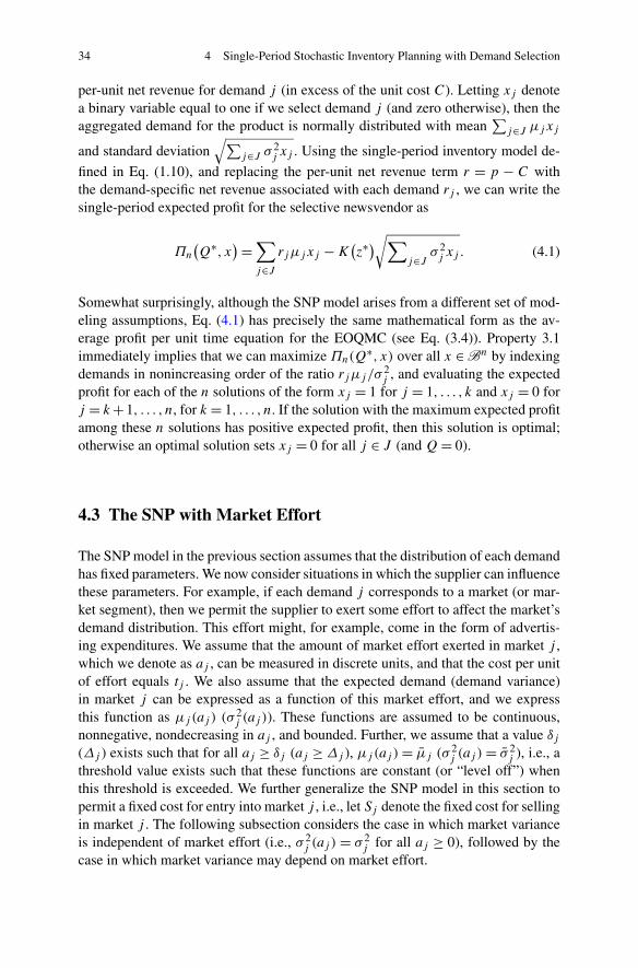
34 4 Single-Period Stochastic Inventory Planning with Demand Selection
per-unit net revenue for demand j (in excess of the unit cost C). Letting xj denotea binary variable equal to one if we select demand j (and zero otherwise), then theaggregated demand for the product is normally distributed with mean
∑j∈J μjxj
and standard deviation√∑
j∈J σ 2j xj . Using the single-period inventory model de-
fined in Eq. (1.10), and replacing the per-unit net revenue term r = p − C withthe demand-specific net revenue associated with each demand rj , we can write thesingle-period expected profit for the selective newsvendor as
Πn
(Q∗, x
) =∑
j∈J
rjμjxj − K(z∗)
√∑
j∈Jσ 2
j xj . (4.1)
Somewhat surprisingly, although the SNP model arises from a different set of mod-eling assumptions, Eq. (4.1) has precisely the same mathematical form as the av-erage profit per unit time equation for the EOQMC (see Eq. (3.4)). Property 3.1immediately implies that we can maximize Πn(Q
∗, x) over all x ∈ Bn by indexingdemands in nonincreasing order of the ratio rjμj/σ
2j , and evaluating the expected
profit for each of the n solutions of the form xj = 1 for j = 1, . . . , k and xj = 0 forj = k + 1, . . . , n, for k = 1, . . . , n. If the solution with the maximum expected profitamong these n solutions has positive expected profit, then this solution is optimal;otherwise an optimal solution sets xj = 0 for all j ∈ J (and Q = 0).
4.3 The SNP with Market Effort
The SNP model in the previous section assumes that the distribution of each demandhas fixed parameters. We now consider situations in which the supplier can influencethese parameters. For example, if each demand j corresponds to a market (or mar-ket segment), then we permit the supplier to exert some effort to affect the market’sdemand distribution. This effort might, for example, come in the form of advertis-ing expenditures. We assume that the amount of market effort exerted in market j ,which we denote as aj , can be measured in discrete units, and that the cost per unitof effort equals tj . We also assume that the expected demand (demand variance)in market j can be expressed as a function of this market effort, and we expressthis function as μj (aj ) (σ 2
j (aj )). These functions are assumed to be continuous,nonnegative, nondecreasing in aj , and bounded. Further, we assume that a value δj
(Δj ) exists such that for all aj ≥ δj (aj ≥ Δj ), μj (aj ) = μj (σ 2j (aj ) = σ 2
j ), i.e., athreshold value exists such that these functions are constant (or “level off”) whenthis threshold is exceeded. We further generalize the SNP model in this section topermit a fixed cost for entry into market j , i.e., let Sj denote the fixed cost for sellingin market j . The following subsection considers the case in which market varianceis independent of market effort (i.e., σ 2
j (aj ) = σ 2j for all aj ≥ 0), followed by the
case in which market variance may depend on market effort.

4.3 The SNP with Market Effort 35
4.3.1 Market Variance Independent of Market Effort
When each market’s variance is independent of market effort, we need to first deter-mine the optimal effort exerted in market j , if we choose market j . This is accom-plished by determining the value of aj that maximizes θj (aj ) = rjμj (aj ) − tj aj .The difficulty of determining this value of aj depends on the functional form ofμj (aj ). If, for example, each function θj (aj ) is differentiable and concave, then asimple first-order condition is all that is required for identifying an optimal value ofaj , denoted by a∗
j . This first-order condition can be written as
dμj (a∗j )
daj
= tj
rj. (4.2)
Letting R∗j = rjμj (a
∗j ) − tj a
∗j − Sj , then we can determine an optimal solution for
the case in which expected demand depends on market effort by maximizing
Πn
(Q∗, x
) =∑
j∈J
R∗j xj − K
(z∗)
√∑
j∈Jσ 2
j xj , (4.3)
over all x ∈ Bn. Clearly (4.3) takes the same form as (4.1), and we can solve thisproblem using the sorting approach we have described based on the ratios R∗
j /σ 2j
for j = 1, . . . , n.
4.3.2 Market Variance Dependent on Market Effort
When each market’s demand variance also depends on the level of market effort,then the functional form of each μj (aj ) and σ 2
j (aj ) function determines the prob-lem’s overall complexity. In [3], specific functional forms are assumed, which maybe characterized as follows. Each expected demand function μj (aj ) is an approx-imate S-curve function that is nonnegative and continuous for all aj ≥ 0, strictlyconvex and increasing in aj for 0 ≤ aj ≤ αj , linearly increasing for αj ≤ aj ≤ δj
(with a slope at least as great as the limit of the derivative of the strictly convex por-tion as aj → αj ), and fixed at μj for aj ≥ δj . The variance function is nonnegative,continuous, concave, and nondecreasing for all aj ≥ 0, with σ 2
j (aj ) = σ 2j for all
aj ≥ Δj for some positive Δj . Under these assumptions, it is shown in [3] that theoptimal effort level in market j , if market j is selected, must equal either 0 or δj .Assuming that the fixed cost of market entry, Sj , is at least as great as the expectednet revenue at zero effort (at aj = 0), then we can set R∗
j = rjμj (δj ) − tj δj − Sj
(which is equivalent to setting a∗j = δj in our approach in the previous subsection),
and apply the same sorting-based solution approach as before, again using the ratioR∗
j /σ 2j .

36 4 Single-Period Stochastic Inventory Planning with Demand Selection
4.4 The SNP with Limited Market Resources
In most situations, resources required for marketing effort are not unlimited. Wetherefore assume that the total amount of market effort is limited by some valueb. For ease of exposition, we assume that μj (0) = 0, σ 2
j (0) = 0, and Sj > 0 for
all j ∈ J .1 Note that this implies Sj > rjμj (0) for all j ∈ J . We also assume thatμj (aj ) is convex and that σ 2
j (aj ) is concave, in addition to the previous assumptionswe have stated regarding these functions. We formulate the SNP with limited marketresources as follows:
[SNPM] Maximize∑
j∈J
(Rj (aj ) − tj aj − Sj
)xj − K
(z∗)
√∑
j∈J
σ 2j (aj )xj
(4.4)
Subject to∑
j∈J
aj ≤ b, (4.5)
xj ∈ {0,1}, ∀j ∈ J, (4.6)
where Rj (aj ) = rjμj (aj ). The SNPM formulation is quite complicated for severalreasons, not the least of which is the presence of the product of continuous functionsof continuous variables and binary variables. Unlike the approach in the previoussection, the aj values are no longer independent, and we cannot, therefore, simplydetermine the optimal value of aj by maximizing θj (aj ) over aj ≥ 0. Our goalis therefore to provide an effective method for efficient solution of the continuousrelaxation of SNPM, which can then be used within a branch-and-bound scheme.
To this end, observe that aj ≤ δj xj is a valid inequality for SNPM for all j ∈ J ,as μj (aj ) = μj for j ≥ δj . We next define a new set of continuous variables wj
for j ∈ J , such that wj = aj/δj , which implies that we can confine our attention tocontinuous values of wj between zero and one, and we can rewrite the SNPM as
Maximize∑
j∈J
(Rj (δjwj ) − tj δjwj − Sjxj
) − K(z∗)
√∑
j∈J
σ 2j (δjwj ) (4.7)
∑
j∈J
δjwj ≤ b, (4.8)
xj ∈ {0,1}, ∀j ∈ J, (4.9)
0 ≤ wj ≤ xj , ∀j ∈ J. (4.10)
We next observe that if we do not select market j , which implies xj = 0, thenan optimal solution exists such that wj = 0, i.e., we can change the right-hand
1For a detailed discussion of the more general case in which μj (0) > 0 and σ 2j (0) > 0, please see
[3].

4.5 The SNP with Pricing 37
side of each constraint in constraint set (4.10) to one without loss of optimality.We can actually demonstrate a stronger result for the continuous relaxation (see[3]). That is, when we relax (4.9) to permit xj ∈ [0,1] for each j ∈ J , then wecan show that an optimal solution exists for this relaxation such that wj = xj ,which is equivalent to aj = δj xj . Next, note that because μj (aj ) is convex, wehave μj (δj xj ) ≤ μj (δj )xj ; similarly, because σ 2
j (aj ) is concave we also have
σ 2j (δj )xj ≤ σ 2
j (δj xj ).As a result, we obtain the following formulation for solving the continuous re-
laxation of SNPM:
Maximize∑
j∈J
Rj (δj )wj − K(z∗)
√∑
j∈J
σ 2j (δj )wj (4.11)
Subject to∑
j∈J
δjwj ≤ b, (4.12)
0 ≤ wj ≤ 1, ∀j ∈ J, (4.13)
where Rj (δj ) = Rj (δj )− tj δj −Sj . The objective function of the above problem isprecisely the same as that of the SNP and EOQMC problems. However, the knap-sack constraint (4.12) complicates the problem and leads to an interesting class ofnonlinear knapsack problems. Unfortunately, this problem is not as nicely structuredas the nonlinear knapsack problems considered in the previous chapter. Despite this,it is possible to solve this relaxation in O(n3) time, as shown in [2]. For a detaileddiscussion of a customized branch-and-bound algorithm for solving SNPM, pleasesee [3].
4.5 The SNP with Pricing
So far in this chapter, we have not considered the impact of pricing on the solution ofthe SNP. We next consider a profit-maximizing model in which prices are decisionvariables. We first consider the case in which no price discrimination is possible,i.e., the price must be the same for every market. We then discuss the problem whenprice discrimination is permitted.
4.5.1 Equal Market Prices
The SNP with equal market prices, which we denote by SNPP=, can be formulatedas follows:
[SNPP=] Maximize∑
j∈J
Rj (p)xj − K(z∗)
√∑
j∈J
σ 2j (p)xj (4.14)
Subject to xj ∈ {0,1}, ∀j ∈ J, (4.15)
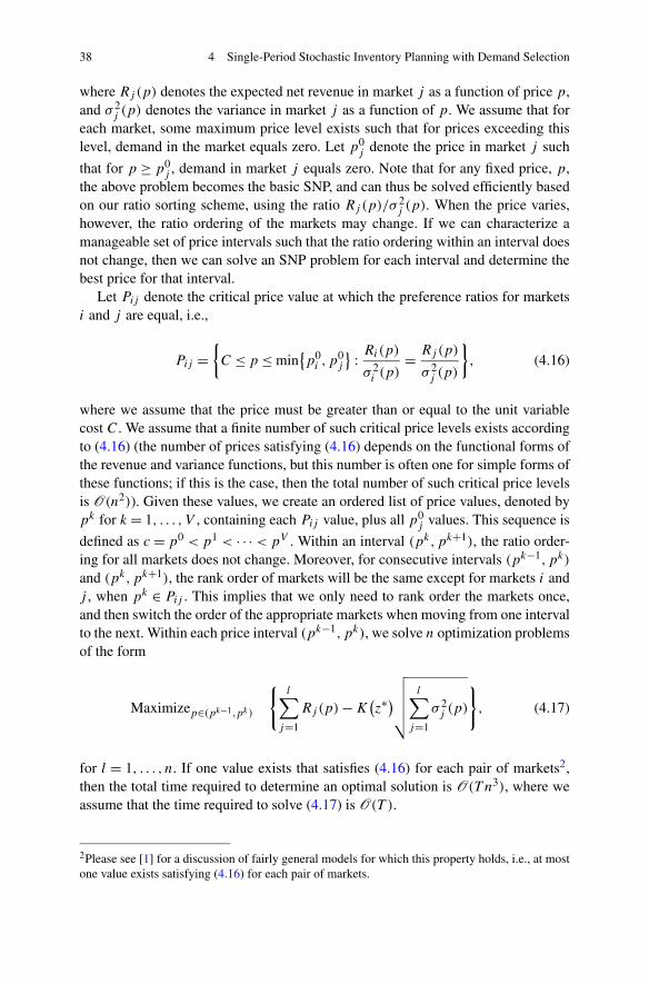
38 4 Single-Period Stochastic Inventory Planning with Demand Selection
where Rj (p) denotes the expected net revenue in market j as a function of price p,and σ 2
j (p) denotes the variance in market j as a function of p. We assume that foreach market, some maximum price level exists such that for prices exceeding thislevel, demand in the market equals zero. Let p0
j denote the price in market j such
that for p ≥ p0j , demand in market j equals zero. Note that for any fixed price, p,
the above problem becomes the basic SNP, and can thus be solved efficiently basedon our ratio sorting scheme, using the ratio Rj (p)/σ 2
j (p). When the price varies,however, the ratio ordering of the markets may change. If we can characterize amanageable set of price intervals such that the ratio ordering within an interval doesnot change, then we can solve an SNP problem for each interval and determine thebest price for that interval.
Let Pij denote the critical price value at which the preference ratios for marketsi and j are equal, i.e.,
Pij ={
C ≤ p ≤ min{p0
i , p0j
} : Ri(p)
σ 2i (p)
= Rj(p)
σ 2j (p)
}
, (4.16)
where we assume that the price must be greater than or equal to the unit variablecost C. We assume that a finite number of such critical price levels exists accordingto (4.16) (the number of prices satisfying (4.16) depends on the functional forms ofthe revenue and variance functions, but this number is often one for simple forms ofthese functions; if this is the case, then the total number of such critical price levelsis O(n2)). Given these values, we create an ordered list of price values, denoted bypk for k = 1, . . . , V , containing each Pij value, plus all p0
j values. This sequence is
defined as c = p0 < p1 < · · · < pV . Within an interval (pk,pk+1), the ratio order-ing for all markets does not change. Moreover, for consecutive intervals (pk−1,pk)
and (pk,pk+1), the rank order of markets will be the same except for markets i andj , when pk ∈ Pij . This implies that we only need to rank order the markets once,and then switch the order of the appropriate markets when moving from one intervalto the next. Within each price interval (pk−1,pk), we solve n optimization problemsof the form
Maximizep∈(pk−1,pk)
{l∑
j=1
Rj(p) − K(z∗)
√√√√√
l∑
j=1
σ 2j (p)
}
, (4.17)
for l = 1, . . . , n. If one value exists that satisfies (4.16) for each pair of markets2,then the total time required to determine an optimal solution is O(T n3), where weassume that the time required to solve (4.17) is O(T ).
2Please see [1] for a discussion of fairly general models for which this property holds, i.e., at mostone value exists satisfying (4.16) for each pair of markets.
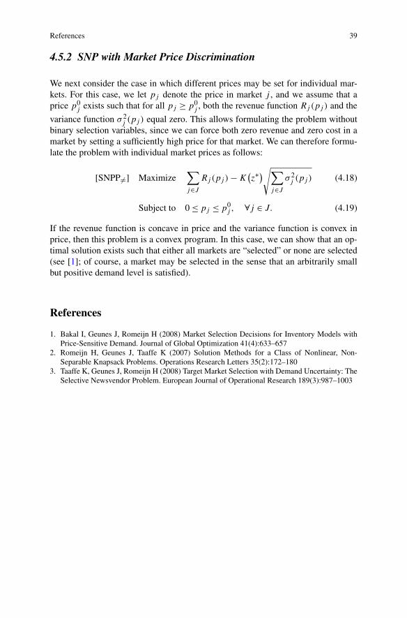
References 39
4.5.2 SNP with Market Price Discrimination
We next consider the case in which different prices may be set for individual mar-kets. For this case, we let pj denote the price in market j , and we assume that aprice p0
j exists such that for all pj ≥ p0j , both the revenue function Rj (pj ) and the
variance function σ 2j (pj ) equal zero. This allows formulating the problem without
binary selection variables, since we can force both zero revenue and zero cost in amarket by setting a sufficiently high price for that market. We can therefore formu-late the problem with individual market prices as follows:
[SNPP�=] Maximize∑
j∈J
Rj (pj ) − K(z∗)
√∑
j∈J
σ 2j (pj ) (4.18)
Subject to 0 ≤ pj ≤ p0j , ∀j ∈ J. (4.19)
If the revenue function is concave in price and the variance function is convex inprice, then this problem is a convex program. In this case, we can show that an op-timal solution exists such that either all markets are “selected” or none are selected(see [1]; of course, a market may be selected in the sense that an arbitrarily smallbut positive demand level is satisfied).
References
1. Bakal I, Geunes J, Romeijn H (2008) Market Selection Decisions for Inventory Models withPrice-Sensitive Demand. Journal of Global Optimization 41(4):633–657
2. Romeijn H, Geunes J, Taaffe K (2007) Solution Methods for a Class of Nonlinear, Non-Separable Knapsack Problems. Operations Research Letters 35(2):172–180
3. Taaffe K, Geunes J, Romeijn H (2008) Target Market Selection with Demand Uncertainty: TheSelective Newsvendor Problem. European Journal of Operational Research 189(3):987–1003

Chapter 5Dynamic Lot Sizing with Demand Selectionand the Pricing Analog
Abstract This chapter defines a model for production planning for a single productin a periodic setting, where the planner must select from a number of individualorders for the product. Associated with any order are a demand quantity, deliveryperiod, and revenue. Acceptance of an order implies that it must be met on time andin full. Orders are placed in advance of the planning horizon, and the planner mustdetermine which orders to accept as well as a production plan for meeting theseorders on time over a finite horizon. Production in any period carries a fixed ordercost as well as variable production costs, and inventory may be held from periodto period, incurring an associated holding cost. The planner’s goal is to maximizeprofit from order acceptance decisions over the planning horizon.
5.1 Demand Selection Problem Definition
The model we consider in this chapter generalizes the ELSP, discussed in Chap. 1,and is intimately related to the ELSP with pricing presented in Chap. 2, as we laterdiscuss in Sect. 5.4. In this section we formally define the demand selection problem(DSP), while the remainder of this chapter provides a solution algorithm (Sect. 5.2),discusses the implications of capacity limits on production (Sect. 5.5), and providesan interpretation of the problem as an equivalent pricing and lot sizing problem(Sect. 5.4). Much of the work presented in this chapter is based on [3].
Consider a single-item production planning problem for a finite planning horizonof length T , where production occurs and demand is realized in a discrete set ofperiods indexed by t . In advance of the planning horizon, a number of demands areavailable, and each of these demands must be either accepted or rejected. Associatedwith demand j in period t are a demand quantity, djt , and a per-unit revenue, rjt ;thus, the total revenue associated with acceptance of demand j in period t equalsrjt djt . We assume without loss of generality that nt demands exist in period t , andthat demands within any period are indexed in non-increasing order of unit revenues,i.e., rjt ≥ rj+1,t , for all t = 1, . . . , T and j = 1, . . . , nt − 1.
Let wjt denote the percentage of demand j in period t that is fulfilled, i.e., wjt isa continuous variable between zero and one (as we later show, an optimal solutionwill exist in which each wjt is strictly zero or one in the absence of capacity lim-its). The total demand that must be met in period t , which depends on the demand
J. Geunes, Demand Flexibility in Supply Chain Planning,SpringerBriefs in Optimization,DOI 10.1007/978-1-4419-9347-2_5, © Joseph Geunes 2012
41
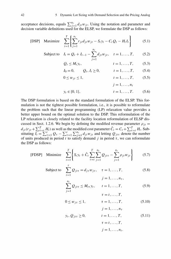
42 5 Dynamic Lot Sizing with Demand Selection and the Pricing Analog
acceptance decisions, equals∑nt
j=1 djtwjt . Using the notation and parameter anddecision variable definitions used for the ELSP, we formulate the DSP as follows:
[DSP] MaximizeT∑
t=1
{nt∑
j=1
rjt djtwjt − Styt − CtQt − HtIt
}
(5.1)
Subject to It = Qt + It−1 −nt∑
j=1
djtwjt , t = 1, . . . , T , (5.2)
Qt ≤ Mtyt , t = 1, . . . , T , (5.3)
I0 = 0, Qt , It ≥ 0, t = 1, . . . , T , (5.4)
0 ≤ wjt ≤ 1, t = 1, . . . , T , (5.5)
j = 1, . . . , nt
yt ∈ {0,1}, t = 1, . . . , T . (5.6)
The DSP formulation is based on the standard formulation of the ELSP. This for-mulation is not the tightest possible formulation, i.e., it is possible to reformulatethe problem such that the linear programming (LP) relaxation value provides abetter upper bound on the optimal solution to the DSP. This reformulation of theLP relaxation is closely related to the facility location reformulation of ELSP dis-cussed in Sect. 1.2.6. We begin by defining the modified revenue parameter ρjt =djt (rjt +∑T
τ=t Ht ) as well as the modified cost parameter Ct = Ct +∑Tτ=t Ht . Sub-
stituting It = ∑tτ=1 Qτ − ∑t
τ=1∑nt
j=1 djtwjt and letting Qjtτ denote the numberof units produced in period t to satisfy demand j in period τ , we can reformulatethe DSP as follows:
[FDSP] MinimizeT∑
t=1
{
Styt + Ct
T∑
τ=t
nt∑
j=1
Qjtτ −nt∑
j=1
ρjtwjt
}
(5.7)
Subject toτ∑
t=1
Qjtτ = djτwjτ , τ = 1, . . . , T , (5.8)
j = 1, . . . , nτ ,nt∑
j=1
Qjtτ ≤ Mtτyt , t = 1, . . . , T , (5.9)
τ = t, . . . , T ,
0 ≤ wjτ ≤ 1, τ = 1, . . . , T , (5.10)
j = 1, . . . , nτ
yt ,Qjtτ ≥ 0, t = 1, . . . , T , (5.11)
τ = t, . . . , T ,
j = 1, . . . , nt .

5.2 Dual Ascent Solution Algorithm 43
The multiplier on the right-hand side of constraint set (5.9), Mtτ , is a large num-ber that ensures the problem remains uncapacitated, and can be replaced withMtτ = ∑nτ
j=1 djτ without loss of optimality. To demonstrate the tightness of theLP relaxation FDSP, the next section provides an algorithm for solving the dual ofFDSP. We then show that the resulting dual has an optimal solution with a comple-mentary primal solution that is feasible for DSP, and therefore optimal. We note thatthis reformulation and dual solution approach follow that shown in [6].
5.2 Dual Ascent Solution Algorithm
This section formulates the dual problem for FDSP and provides an algorithm forsolving this dual problem. We first define dual multipliers μjτ , ωtτ , and πjτ as-sociated with primal constraints (5.8), (5.9), and the upper bounding constraints of(5.10). We can then formulate the dual problem, DP, as follows:
[DP] MaximizeT∑
τ=1
nt∑
j=1
−πjτ (5.12)
Subject toT∑
τ=t
nt∑
j=1
djτωtτ ≤ St , t = 1, . . . , T , (5.13)
djτμjτ + πjτ ≥ ρjτ , τ = 1, . . . , T , j = 1, . . . , nτ
(5.14)
μjτ − ωtτ ≤ Ct , t = 1, . . . , T , τ = t, . . . , T ,
(5.15)j = 1, . . . , nt ,
πjτ ,ωtτ ≥ 0,μjτ unrestricted, t = 1, . . . , T , τ = t, . . . , T ,
(5.16)j = 1, . . . , nt .
We observe from (5.15) that an optimal solution will exist such that ωtτ is equal tothe maximum between zero and μjτ − Ct for all t , τ , and j . In addition, because ofthe form of the objective and constraint set (5.14), at optimality, we will have −πjτ
equal to the minimum between zero and djτμjτ − ρjτ for every j and τ . Based onthese observations, we can formulate DP much more compactly as follows:
[CDP] MaximizeT∑
τ=1
nt∑
j=1
min{0, djτμjτ − ρjτ } (5.17)
Subject toT∑
τ=t
nt∑
j=1
djτ
(max{0,μjτ − Ct }
) ≤ St , t = 1, . . . , T .
(5.18)

44 5 Dynamic Lot Sizing with Demand Selection and the Pricing Analog
Inspection of CDP leads to some interesting and useful observations. Note first thatan optimal solution exists such that μjτ is no greater than ρjτ /djτ for every j, τ
pair. Thus, for any j, τ pair such that mint=1,...,τ Ct ≥ ρjτ /djτ , the variable μjτ
can be set to its maximum value of ρjτ /djτ without consuming any constraint “ca-pacity,” which implies that we can eliminate such variables from the formulationimmediately. Next, note that we can start with an initial feasible solution that setsμjτ = mint=1,...,τ Ct for every j, τ pair. This initial solution does not consume anyof the capacity of any of the constraints (5.18). Beginning with this initial solution,we will increase values of the μjτ variables in a specific order, resulting in what iscommonly called a dual ascent algorithm.
This algorithm begins by simultaneously increasing the values of all μj1 vari-ables from their initial value of C1. That is, we create a set J 1
1 containing all ordersin period 1 that have not been eliminated. Increasing these variables consumes someof the capacity, S1, of constraint 1, but does not affect any of the other constraints,as the μj1 variables appear only in the first constraint. If μk1 hits the value ρk1/dk1
before constraint 1 becomes tight, then we remove order k from the set J 11 , insert
order k into the set J 01 , and we do not continue to increase the value of μk1 with
the other μj1 variables such that j ∈ J 11 . We continue simultaneously increasing the
μj1 values for all j ∈ J 11 , until either J 1
1 = ∅ or until the variables consume all ofthe capacity of constraint 1. We therefore have
μj1 =
⎧⎪⎨
⎪⎩
ρj1dj1
, j ∈ J 01 ,
C1 +S1−∑
j∈J01
dj1 max{0,ρj1/dj1−C1}∑
j∈J11
dj1, j ∈ J 1
1 .(5.19)
We next move on to period 2, by inserting all orders in period 2 in the set J 12 , and
simultaneously increasing the values of all μj2 variables for j ∈ J 12 . A variable μk2
may be blocked from further increase because (a) it hits the value ρk2/dk2, in whichcase order k is removed from J 1
2 and inserted in the set J 02 ; (b) constraint 2 becomes
tight; or (c) it hits the value C1 (and any further increase would violate constraint 1).At this point we have
μj2 =
⎧⎪⎨
⎪⎩
ρj2dj2
, j ∈ J 02 ,
min{C1; C2 +S2−∑
j∈J02
dj2 max{0,ρj2dj2
−C2}∑
j∈J12
dj2}, j ∈ J 1
2 .(5.20)
We continue this approach for subsequent periods. In general, for period t , if J 1t �= ∅,
then letting [x]+ = max{0, x}, we can write the value of μkt for k ∈ J 1t using the
formula
μ∗t = min
s≤t
{
Cs +Ss − ∑t
τ=s
∑j∈J 0
tdjτ
[ρjτ
djτ− Cs
]+ − ∑t−1τ=s
∑j∈J 1
τdjτ [μ∗
τ − Cs ]+∑
j∈J 1t
dj t
}
,
(5.21)
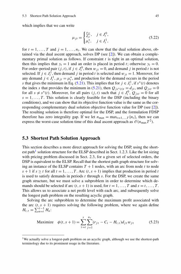
5.3 Shortest Path Solution Approach 45
which implies that we can write
μjt ={
ρjt
djt, j ∈ J 0
t ,
μ∗t , j ∈ J 1
t ,(5.22)
for t = 1, . . . , T and j = 1, . . . , nt . We can show that the dual solution above, ob-tained via the dual ascent approach, solves DP (see [2]). We can obtain a comple-mentary primal solution as follows. If constraint t is tight in an optimal solution,then this implies that yt = 1 and an order is placed in period t ; otherwise yt = 0.For order–period pair (j, t), if j ∈ J 0
t , then wjt = 0, and demand j in period t is notselected. If j ∈ J 1
t , then demand j in period t is selected and wjt = 1. Moreover, forany demand j ∈ J 1
t , μjt = μ∗t , and production for the demand occurs in the period
s that gives the minimum in Eq. (5.21). This implies that for j ∈ J 1t , if s∗(t) denotes
the index s that provides the minimum in (5.21), then Qjs∗(t)t = djt , and Qjst = 0for all s �= s∗(t). Moreover, for all pairs (j, t) such that j ∈ J 0
t , Qjst = 0 for alls = 1, . . . , T . This solution is clearly feasible for the DSP (including the binaryconditions), and we can show that its objective function value is the same as the cor-responding complementary dual solution objective function value for DP (see [2]).The resulting solution is therefore optimal for the DSP, and the formulation FDSPtherefore has zero integrality gap. If we let nmax = maxt=1,...,T {nt }, then we canexpress the worst-case solution time of this dual ascent approach as O(nmaxT
2).
5.3 Shortest Path Solution Approach
This section describes a more direct approach for solving the DSP, using the short-est path1 solution structure for the ELSP described in Sect. 1.2.3. Like the lot sizingwith pricing problem discussed in Sect. 2.3, for a given set of selected orders, theDSP is equivalent to the ELSP. Recall that the shortest path graph structure for solv-ing an instance of the ELSP contains T + 1 nodes, with an arc from node t to nodes + 1 if s ≥ t for all t = 1, . . . , T . Arc (t, s + 1) implies that production in period t
is used to satisfy demands in periods t through s. For the DSP, we create the samegraph structure, but we must solve a subproblem in order to determine which de-mands should be selected if arc (t, s + 1) is used, for t = 1, . . . , T and s = t, . . . , T .This allows us to associate a net profit level with each arc, and subsequently solvethe longest path problem on the resulting acyclic graph.
Solving the arc subproblem to determine the maximum profit associated withthe arc (t, s + 1) requires solving the following problem, where we again defineHt,τ = ∑τ−1
u=t Hu:
Maximize φ(t, s + 1) =s∑
τ=t
nτ∑
j=1
(rjτ − Ct − Ht,τ )djτwjτ (5.23)
1We actually solve a longest-path problem on an acyclic graph, although we use the shortest-pathterminology due to its prominent usage in the literature.

46 5 Dynamic Lot Sizing with Demand Selection and the Pricing Analog
Subject to wjτ ∈ {0,1}, τ = t, . . . , s, j = 1, . . . , nτ . (5.24)
For the given arc (t, s + 1), clearly we will select demand j in period τ such thatt ≤ τ ≤ s if rjτ > Ct + Ht,τ , i.e., if the unit revenue exceeds the variable costsassociated with the demand. If the optimal solution to the above subproblem, whichwe denote as φ∗(t, s + 1), exceeds the fixed order cost St , then the arc is assigned anet profit of φ∗(t, s + 1) − St . Otherwise, the arc is assigned a net profit of zero.
This solution approach is much easier to describe than the dual ascent method,although its complexity is the same, equal to O(nmaxT
2). The dual ascent method,however, enables demonstrating that the FDSP formulation has zero integrality gap,i.e., that this formulation is tight.
5.4 Interpretation of the DSP as a Pricing Problem
Recall that the ELSP with pricing problem described in Sect. 2.3 assumed that de-mand in each period was price dependent, using the function Dt(pt ) to express de-mand in period t as a function of the price in period t , pt . The total revenue in thismodel, contained in the first term of the objective function of [ELSP′], was equal toptDt (pt ). For many common forms of the demand function, Dt(pt ), the resultingrevenue function, equal to ptDt(pt ), is a concave function (for example, when thedemand function is linear in price). If we have a one-to-one correspondence betweenthe price in period t and the demand in period t , then, without loss of generality, wecan express the revenue function in a period as a function of either the price or thedemand in period t . If we choose the latter, then we can write the revenue functionin period t as the function Rt(Dt ). That is, replacing Dt(pt ) with Dt and replacingptDt (pt ) with Rt(Dt) in the formulation ELSP′ in Sect. 2.3 results in an equiva-lent formulation in the demand variables. This reformulation may be expressed asfollows:
[ELSP′(D)] MaximizeT∑
t=1
{Rt(Dt ) − Styt − CtQt − HtIt
}(5.25)
Subject to It = Qt + It−1 − Dt, t = 1, . . . , T , (5.26)
Qt ≤ Mtyt , t = 1, . . . , T , (5.27)
Qt, It ,Dt ≥ 0, t = 1, . . . , T , (5.28)
yt ∈ {0,1}, t = 1, . . . , T . (5.29)
Suppose that we can approximate the revenue function in any period t as a piece-wise linear, concave, and nondecreasing function of the demand level in period t ,with nt + 1 segments. Letting rjt denote the slope of segment j of the revenuefunction in period t , and assuming rjt > rj+1,t , then we can express this revenue

5.5 Capacitated Versions 47
function as
Rt(Dt ) =
⎧⎪⎨
⎪⎩
∑k−1j=1 rjtdjt + rkt (Dt − ∑k−1
j=1 djt ),∑k−1
j=1 djt ≤ Dt <∑k
j=1 djt ,
k = 1, . . . , nt ,∑nt
j=1 rjtdjt , Dt ≥ ∑nt
j=1 djt .
(5.30)Using this form of the revenue function in the lot sizing and pricing problemELSP′(D), then, for the subproblem corresponding to arc (t, s + 1), according toEq. (2.15), we need to solve
[PSP(D)] Maximizes∑
τ=t
{Rτ (Dτ ) − (Ct + Ht,τ )Dτ
}. (5.31)
To model the revenue functions shown in Eq. (5.30), we create a binary variablewjτ associated with the j th linear segment of the revenue function in period τ ,for τ = 1, . . . , T , and j = 1, . . . , nτ + 1. The resulting arc profit subproblem takesthe exact form of (5.23)–(5.24) (with an additional zero-slope segment for everyperiod). Observe that because we are maximizing, we need not impose explicit con-straints on the selection of different linear segments associated with the revenuefunction in any given period, i.e., an optimal solution will select segments in nonin-creasing order of segment slopes. Thus, this special case of the ELSP with pricingand piecewise linear and concave revenue functions is equivalent to the DSP.
Before proceeding we note two additional properties of the arc subproblem[PSP(D)] (which also hold for the arc subproblem expressed in (5.23)–(5.24), asthese problems are equivalent) for any arc (t, s + 1). First, note that explicit binaryrestrictions on the wjτ variables are not required, as an optimal solution will existfor the continuous relaxation such that each wjτ takes a value of zero or one. In par-ticular, an optimal solution exists such that wjτ = 1 for every pair (j, τ ) such thatrjτ > Ct + Ht,τ , and wjτ = 0 for every (j, τ ) such that rjτ ≤ Ct + Ht,τ . This leadsto the second property, which states that for arc (t, s + 1) and for period τ such thatt ≤ τ ≤ s, the generalized first-order condition for (5.31) is necessary and sufficientfor optimality, i.e., Ct +Ht,τ ∈ ∂Rτ (Dτ ), where ∂Rτ (Dτ ) is the set of subgradientsof the function Rτ (Dτ ) at Dτ . However, this condition is equivalent to the conditionthat if r(k+1)τ ≤ Ct + Ht,τ ≤ rkτ , then Ct + Ht,τ ∈ ∂Rτ (
∑kj=1 djτ ), and an optimal
solution exists for the arc (t, s + 1) subproblem such that wjτ = 1 for j = 1, . . . , k
and wjτ = 0 for j = k + 1, . . . , nτ + 1.
5.5 Capacitated Versions
Our analysis in this chapter thus far has assumed that no limit exists on the sizeof any production/procurement order. In contexts in which production/procurementorders are limited by some capacity level (which includes virtually all practical con-texts), the DSP becomes more difficult. Formulating the capacitated version of the

48 5 Dynamic Lot Sizing with Demand Selection and the Pricing Analog
problem requires simply replacing each big-M value (Mt ) in the DSP formulationwith the associated finite capacity level, denoted as bt , for t = 1, . . . , T . We de-note the capacitated demand selection problem by CDSP, and note that, based onthe results in the prior section, an equivalent lot sizing with pricing problem withpiecewise-linear and concave revenue functions exists. We also observe that, unlikethe DSP, the CDSP is an N P-Hard optimization problem, as it contains the ca-pacitated lot sizing problem as a special case. In this section we will briefly discussmodeling issues and problem variants of the CDSP.
Recall that in the DSP formulation it did not matter whether the demand selec-tion (wjt ) variables were required to take binary values. That is, even though weformulated the problem such that these variables were free to take any values be-tween zero and one, an optimal solution exists such that each of these variables willbe binary at optimality. When finite production capacities exist, however, this is notthe case, and whether or not we require these variables to take binary values has asubstantial impact on the difficulty of the problem. Moreover, contexts may exist(particularly when capacities are limited) in which not all orders are completely ful-filled, but some are partially fulfilled. We therefore classify capacitated versions ofthe CDSP according to two important factors. The first of these factors is whetheror not partial order fulfillment is permissible. When partial order fulfillment is per-missable, the demand selection (wjt ) variables are free to take any values betweenzero and one. If partial order satisfaction is not permitted, then these variables mustbe binary. The second factor corresponds to whether or not the finite productioncapacity parameters vary with time. In the equal-capacity case, capacity equals b
in every time period, whereas in the general case we retain the subscript on bt toindicate capacity values that are time-varying.
Although, as noted previously, the CDSP is N P-Hard, the special case withcontinuous demand selection variables and time-invariant capacities can be solved inpolynomial time, based on the polynomial solvability of the equal-capacity lot sizingproblem (see [1, 5]). That is, as with the uncapacitated DSP, because the associatedproblem is polynomially solvable for any given demand vector, and because thedemands (orders) in different periods are independent of one another, this specialcase of the CDSP is polynomially solvable. We next briefly sketch the propertiesthat facilitate its solution in polynomial time.
As with the uncapacitated DSP, an optimal solution exists for the CDSP withequal capacities consisting of a sequence of regeneration intervals. A regenerationinterval is a subsequence of time periods t through s with 1 ≤ t ≤ s ≤ T , such thatno inventory is held at the end of periods t −1 and s, but a positive level of inventoryis held at the end of periods t, t + 1, . . . , s − 1. For the DSP, each arc we defined inthe shortest path solution approach corresponded to a regeneration interval, and forthe uncapacitated problem, all production in the regeneration interval occurred inthe first period (t) of the regeneration interval (defined by the arc (t, s + 1)). In theequal-capacity version of the lot sizing problem, production within a regenerationinterval may occur in any of the periods. However, an optimal solution exists suchthat, within any regeneration interval, the production level equals either zero or thecapacity level b for all periods except at most one (see [1]).

5.5 Capacitated Versions 49
To illustrate why this implies polynomial solvability for the ELSP with constantcapacities, note that if we have a regeneration interval (t, s + 1), this implies thatIt−1 = 0, Is = 0, and Iτ > 0 for τ = t, t + 1, . . . , s − 1. Because of this, produc-tion in periods t through s must satisfy all demands in periods t through s. LettingD(t, s) = ∑s
τ=t Dτ , then if the total production in periods t through s must equalD(t, s), and if production must equal zero or b for all periods except at most one,then we know that the amount produced in the period in which we do not produceat zero or b must equal D(t, s) mod b, where x mod y = x − yx/y. As a result,when solving the subproblem for arc (t, s + 1), we only need to consider solutionsthat (a) produce either zero, b, or D(t, s) mod b in each period, and (b) ensure thatcumulative production is at least as great as cumulative demand. As a result, forthe equal-capacity ELSP, the arc subproblem can be solved in polynomial time, andbecause the number of arcs is polynomial in T , the overall problem is polynomiallysolvable.
For the equal-capacity CDSP, these same properties hold for any given demandvector within a regeneration interval, although the number of potential demand vec-tors is effectively infinite (thus, we do not know the value of D(t, s) a priori).A more general characterization of the structural properties of an optimal regen-eration interval solution does, however, exist (see [3]). In particular, it is possible toshow that an optimal regeneration interval exists that is one of the following types:
1. Production in each period in the regeneration interval equals either 0 or b, and atmost one demand is partially satisfied.
2. No demands are partially satisfied, and production may be strictly between 0 andb in at most one period in the regeneration interval.
For any given regeneration interval (t, s + 1), we sort all demands in periods t
through s in nonincreasing order of ρj t = ρjt/djt values. We can show that ifρj t ≥ ρkt ′ for demands j and k in periods t and t ′ within the regeneration inter-val, if an optimal solution exists with wjt < 1, then an optimal solution exists withwkt ′ = 0; similarly, if wkt ′ > 0 then wjt = 1. That is, within any regeneration inter-val we have a preference ordering of the attractiveness of demands. Then, after sort-ing in this order, we can evaluate solutions of type 1 above by going down this listand successively assuming that a particular demand is the one such that 0 < wjt < 1.If a given demand is fractionally satisfied, then all lower indexed demands are fullysatisfied, while all higher indexed demands are not satisfied at all. The choice ofa particular demand to be satisfied fractionally therefore uniquely determines thenumber of periods that must be satisfied at full capacity b (assuming djt < b for allorders), and, as a result, the values of the corresponding wjt variables within theregeneration interval.
For the second type of solution above, given the preference ordering within anyregeneration interval, we may consider a total of O(nmaxT ) solutions such that de-mands 1 through l have wjt = 1, while the remaining demands have wjt = 0. Eachsuch solution implies a value of D(t, s), as well as the number of periods in whichproduction must be at full capacity. We thus have a polynomial number of solutionsof types 1 and 2 above that need to be evaluated for each regeneration interval. The

50 5 Dynamic Lot Sizing with Demand Selection and the Pricing Analog
time required to determine an optimal subproblem solution is the time required tosolve an equal-capacity lot sizing problem (which is O(T 3)) for at most O(nmaxT )
demand vectors. This implies that the time required to find an optimal regenerationinterval solution is O(nmaxT
4). Because there are O(T 2) regeneration intervals, theoverall time required to solve the equal-capacity CDSP is O(nmaxT
6).Unfortunately, when we do not permit partial order satisfaction, the resulting
problem remains N P-Hard, even when all capacities are equal (see [3]). Methodsfor strengthening the LP relaxation as well as heuristic solution approaches for thiscase and problems with time-varying capacities are discussed in [4].
References
1. Florian M, Klein M (1971) Deterministic Production Planning with Concave Costs and Capac-ity Constraints. Management Science 18:12–20
2. Geunes J, Romeijn H, Taaffe K (2004) Order Selection, Pricing, and Lot Sizing: Models andSolution Algorithms. Technical report 2004-2, Industrial and Systems Engineering Department,University of Florida, Gainesville, FL
3. Geunes J, Romeijn H, Taaffe K (2006) Requirements Planning with Pricing and Order SelectionFlexibility. Operations Research 54(2):394–401
4. Taaffe K, Geunes J (2004) Models for Integrated Customer Order Selection and RequirementsPlanning Decisions under Limited Production Capacity, in Supply Chain and Finance (PardalosP, Migdalas A, Baourakis G (eds.)) World Scientific, Singapore
5. Van Hoesel C, Wagelmans A (1996) An O(T 3) Algorithm for the Economic Lot-Sizing Prob-lem with Constant Capacities. Management Science 42(1):142–150
6. Wagelmans A, van Hoesel S, Kolen A (1992) Economic Lot Sizing: An O(n logn) AlgorithmThat Runs in Linear Time in the Wagner-Whitin Case. Operations Research 40(S1):S145–S156

Chapter 6Dynamic Lot Sizing with Market Selection
Abstract This chapter considers a seemingly innocuous change in the assump-tions underlying the Demand Selection Problem (DSP) considered in the previ-ous chapter, which severely complicates the problem analysis. Instead of a se-quence of independent demands over a time horizon, in this variant of the prob-lem, demands in successive periods may be related in the sense that if we satisfya given demand in some period t , we must then satisfy a particular set of de-mands in other periods. That is, instead of selecting individual demands, we arenow faced with the problem of selecting from a set of time-phased vectors of de-mands. In practical terms, this corresponds to determining whether we will satisfyall or none of a given customer’s or market’s demands over the time horizon. Werefer to the resulting problem as the Market Selection Problem (MSP) and discussthe problem’s complexity and potential solution approaches throughout this chap-ter.
6.1 Market Selection Problem Definition
The Market Selection Problem (MSP) considers a set J of n markets, where thedemand from market j in period t equals djt for all j ∈ J and t = 1, . . . , T . We canformulate the MSP as a restriction of a special case of the DSP from the previouschapter. That is, starting with the DSP formulation, we assume that nt = n for all t =1, . . . , T , where n corresponds to the number of markets. We then impose a new setof constraints that require wjt = wjt+1, for all j ∈ J and t = 1, . . . , T −1. That is, ifwe choose to satisfy the demand for market j in any period, we must then satisfy thatmarket’s demand in every period. This is equivalent to eliminating the time subscripton the wjt variables, and we therefore define wj as a binary variable equal to one ifwe satisfy market j demand in all periods, and zero otherwise. We also define Rj asthe total revenue available from market j over the T -period horizon, where, usingthe notation defined in the previous chapter, Rj = ∑T
t=1 rjt djt . We retain the basicnotation and cost assumptions of the DSP except where noted. We can formulate theMSP as follows:
J. Geunes, Demand Flexibility in Supply Chain Planning,SpringerBriefs in Optimization,DOI 10.1007/978-1-4419-9347-2_6, © Joseph Geunes 2012
51

52 6 Dynamic Lot Sizing with Market Selection
[MSP] Maximizen∑
j=1
Rjwj −T∑
t=1
{Styt + CtQt + HtIt } (6.1)
Subject to It = Qt + It−1 −n∑
j=1
djtwj , t = 1, . . . , T , (6.2)
Qt ≤ Mtyt , t = 1, . . . , T , (6.3)
I0 = 0, Qt , It ≥ 0, t = 1, . . . , T , (6.4)
wj ∈ {0,1}, j = 1, . . . , n, (6.5)
yt ∈ {0,1}, t = 1, . . . , T . (6.6)
Observe that we can set Mt = ∑Tτ=t
∑nj=1 djτ in (6.3) without loss of optimality.
For any given selection of markets, the MSP becomes an ELSP, and is, therefore,easily solved. Similarly, for a given production plan, the problem is easily solved aswell. To see this, consider a fixed production plan with v demands placed in periods{1 = t1 < t2 < · · · < tv ≤ T }. Because an optimal solution exists satisfying the ZIOproperty (see Sect. 1.2.3), we know that
Qtl =τl+1−1∑
τ=tl
n∑
j=1
djτwj , l = 1, . . . , v, and (6.7)
It =τl+1−1∑
τ=t+1
n∑
j=1
djτwj , tl ≤ t < tl + 1, l = 1, . . . , v. (6.8)
We can therefore write the net profit associated with a given production plan as
n∑
j=1
(
Rj −v∑
l=1
{
Ctl
τl+1−1∑
τ=tl
djτ +τl+1−2∑
τ=tl
Hτ
τl+1−1∑
u=τ+1
dju
})
wj −r∑
l=1
Stl . (6.9)
We can maximize (6.9) over all binary vectors w by setting wj = 1 if and only if
Rj ≥v∑
l=1
{
Ctl
τl+1−1∑
τ=tl
djτ +τl+1−2∑
τ=tl
Hτ
τl+1−1∑
u=τ+1
dju
}
. (6.10)
Note that the right-hand side of (6.10) corresponds to the total variable cost incurredwhen serving market j using the given production plan with v demands placedin periods {1 = t1 < t2 < · · · < tv ≤ T }. Thus, this condition simply requires thata market’s revenue is at least as great as the associated variable cost incurred inserving the market using the given production plan.
Despite the fact that the problem is easily solved for a given binary vector w orfor a given binary vector y, the problem is unfortunately not easily solved whenboth of these vectors are decision vectors, as we next discuss.

6.1 Market Selection Problem Definition 53
6.1.1 MSP Problem Complexity
The decision version of the MSP was shown to be strongly N P-Complete in [7].Although the complete proof of this result is quite involved, here we sketch theproof structure and the main results involved in the proof. We begin by consideringa very simple special case of the MSP with an odd number of planning periods T ,a fixed order cost of St = 2 in every period, zero variable production cost in everyperiod (all Ct = 0), and a holding cost of one in every period (Ht = 1). Consideran instance of the ELSP with these cost parameters and with a demand of dt = 1in every period. For this ELSP instance, if v = (T − 1)/2, then an optimal solutioncontains v + 1 production orders, where v of the orders cover two periods and oneof the orders covers one period. The average cost per period of this solution (whichalso equals the average cost per unit of demand), AC∗(T ), equals 3/2 + 1/(2T ),which clearly exceeds 3/2.
We next construct a set of markets, such that in every period t = 1, . . . , T , exactlyone market has a demand of one unit, and all other markets have a demand of zerounits in the period. The revenue associated with market j is defined as
Rj = AC∗(T )
T∑
t=1
djt . (6.11)
Let Js ⊆ J denote a set of selected markets such that wj = 1 for j ∈ Js , and letΠ(Js) denote the profit associated with the set Js . Now note that Π(∅) = 0 andΠ(J ) = 0, i.e., selecting either zero markets or all markets produces a profit ofzero. Observe also that any selection of markets results in a time-phased demandvector that is binary, and let D(Js) denote this vector when the subset Js of marketsis selected. We can thus view any such vector D(Js) as a sequence of zeros andones.
Suppose this vector D(Js) contains a subsequence with a zero, followed by anodd number of ones, followed by a zero (for convenience we assume zero demandin dummy periods 0 and T + 1). If this is the case, then if k is the total num-ber of ones in the sequence, under our cost assumptions, the total cost equals atleast (3/2)k + (1/2). The profit associated with this sequence is no greater thanAC∗(T )k − ((3/2)k + (1/2)), which is strictly less than AC∗(T )T − ((3/2)T +(1/2)) = 0. If, instead, all subsequences of consecutive ones correspond to an evennumber of periods, then the optimal production plan always uses an order to satisfytwo consecutive periods worth of demand, which implies that the average cost perunit produced equals (3/2). In this case, if there are k total ones in the vector D(Js),the associated profit equals (AC∗(T ) − (3/2))k > 0. As a result, a solution with netprofit greater than zero exists if and only if the vector D(Js) contains only evensubsequences of consecutive ones. This implies that the MSP is at least as difficultas the problem of determining whether a selection of markets exists for this specialcase satisfying this even subsequence property. This even subsequence problem maybe posed as follows.

54 6 Dynamic Lot Sizing with Market Selection
Consider a set J of n binary vectors, each of dimension T , such that for at mostone of these vectors, element t equals one. Given a subset Js ⊆ J , let D(Js) de-note a (T + 2)-dimensional vector such that elements 1 and T + 2 equal zero, andelements 2 through T + 1 consist of the component-wise sum of the vectors in Js .Note that D(Js) must also be a binary vector. We wish to determine whether a subsetJs exists such that every consecutive sequence of ones in D(Js) is of even length.The remainder of the proof, detailed in [7], involves a reduction from the classical3-Satisfiability problem (3SAT; see [1]) to this even subsequence problem. In par-ticular, we consider the market selection recognition problem, which asks whethera selection of markets exists with net profit greater than B for some constant B .Given any instance of 3SAT, [1] creates an equivalent instance of the market se-lection recognition problem in polynomial time. Thus, if we can answer yes to themarket selection recognition problem in polynomial time, this implies that we cananswer yes to the question of whether the instance of 3SAT is satisfiable in polyno-mial time, which only holds if P = N P .
6.1.2 MSP Approximability
Because it is not possible to find an optimal solution for an N P-Hard problemin polynomial time (unless P = N P), for such problems, researchers often seekso-called approximation algorithms. An approximation algorithm provides a fea-sible solution in polynomial time that adheres to a certain provable performanceguarantee. For instance, if Π∗ denotes the maximum profit of an instance of theMSP, an approximation algorithm A is defined as a 1 − ε approximation algorithmfor a maximization problem if it is guaranteed to produce a solution with profitΠA such that ΠA ≥ (1 − ε)Π∗. Unfortunately, as shown in [7], a 1 − ε approxi-mation algorithm cannot exist for MSP with 0 < ε < 1 unless P = N P . To seethis, suppose that such an algorithm does exist. Recall that in our discussion of theN P-Completeness proof in the previous section, if no profitable market selectionexists (i.e., no selection satisfying the even subsequence property), then Π∗ = 0.This also implies that the corresponding instance of 3SAT is not satisfiable. If suchan approximation algorithm exists, then it is guaranteed to find a solution such thatΠA ≥ (1 − ε)Π∗ = 0, which implies ΠA = 0. If, on the other hand, Π∗ > 0, thenthe corresponding instance of 3SAT is indeed satisfiable, and the approximationalgorithm finds a solution such that ΠA ≥ (1 − ε)Π∗ > 0, i.e., ΠA > 0. But thisimplies that the approximation algorithm can verify, in polynomial time, whetherthe instance of 3SAT is satisfiable, which would imply that 3SAT is polynomiallysolvable (we thus have a contradiction, unless P = N P).
Suppose that we instead consider an alternate approach to formulating the MSP,as discussed in [2] and [4]. In particular, suppose that we view Rj as the opportunitycost for not satisfying market j demand, and let wj = 1 − wj . Thus, if wj = 1,we forgo the revenue associated with market j demand and we need not satisfymarket j demand. We also reformulate the constraint set using a facility location

6.1 Market Selection Problem Definition 55
type of reformulation of the constraint set of the MSP. That is, we let xjtτ denotethe percentage of market j demand in period τ satisfied using production in periodt , and we define c
jtτ = (Ct + ∑τ−1
s=t Hs)djt as the cost to satisfy market j demandin period τ using production in period t . Then we can formulate the LP relaxationof the MSP as follows:
[MSP-alt] Minimizen∑
j=1
Rj wj +T∑
t=1
{
Styt +n∑
j=1
T∑
τ=t
cjtτ xjtτ
}
(6.12)
Subject toτ∑
t=1
xjtτ + wj = 1, τ = 1, . . . , T , (6.13)
j ∈ J,
xjtτ ≤ yt , t = 1, . . . , T , (6.14)
τ = t, . . . , T ,
j ∈ J,
xjtτ , yt ≥ 0, t = 1, . . . , T , (6.15)
τ = t, . . . , T ,
j ∈ J.
The first term of the objective function (6.12) corresponds to the market rejectioncosts, while the remaining terms in brackets are the associated lot sizing costs. Con-sider an optimal solution (w, x, y) for the MSP-alt formulation. Now suppose thatfor any market such that wj ≥ 1/2, we set wj = 1, and for all other markets, we setw = 0. Let J1/2 = {j : wj ≥ 1/2}; this implies that wj = 1 for j ∈ J1/2 and wj = 0for j ∈ J\J1/2. We refer to the resulting w as the rounded LP relaxation marketselection vector, and we denote this vector as wr .
The rejection cost associated with the rounded market selection vector wr
equals∑
j∈J1/2Rj . The rejection cost associated with the LP relaxation solu-
tion equals∑
j∈J Rj wj , and we have 2 × ∑j∈J1/2
Rjwj ≥ ∑j∈J1/2
Rj and 2 ×∑
j∈J\J1/2Rj wj ≥ 0, which implies that
∑j∈J1/2
Rj ≤ 2 × ∑j∈J Rj wj . That is,
the rejection cost of the rounded market selection vector is at most twice the rejec-tion cost associated with the LP relaxation solution.
We next demonstrate that by solving the ELSP that results when fixing w = wr ,we arrive at a feasible solution for the MSP with total cost no greater than twicethe cost of the LP relaxation of MSP-alt. Because the LP relaxation of MSP-altprovides a lower bound on the optimal solution of the MSP, this implies we canobtain a feasible solution for the MSP with cost at most twice that of the optimalsolution.
Let ELSP(1/2) denote the instance of the ELSP that results when the vector w isfixed at wr . When we solve MSP-alt with w = wr , we know that an optimal solutionexists for the resulting LP relaxation with lot sizing costs equal to the optimal so-lution value of ELSP(1/2) (because no integrality gap exists for this formulation of

56 6 Dynamic Lot Sizing with Market Selection
the ELSP). Thus, if we can find a solution to the restricted version of MSP-alt whenw = wr with lot sizing costs at most twice those associated with the LP relaxationsolution (w, x, y), then we know that ELSP(1/2) has an optimal solution value nomore than twice the lot sizing costs associated with (w, x, y). This implies that thetotal rejection plus lot sizing costs of the feasible solution we have constructed areno more than twice the LP relaxation solution.
For j ∈ J1/2, let xjtτ = 0 for all t = 1, . . . , T and τ = t, . . . , T . For j ∈ J\J1/2,
let xj tτ = xj tτ
1−wj, and for every t = 1, . . . , T , let yt = max{minj∈J\J1/2{ yt
1−wj},1}.
Note that this solution is feasible for MSP-alt and that for j ∈ J\J1/2, we havexj tτ ≤ 2xj tτ for all t = 1, . . . , T and τ = t, . . . , T , and for t = 1, . . . , T , yt ≤ yt .Letting x, y denote an optimal solution for ELSP(1/2), we then have
T∑
t=1
{
St yt +n∑
j=1
T∑
τ=t
cjtτ xj tτ
}
≤T∑
t=1
{
St yt +n∑
j=1
T∑
τ=t
cjtτ xj tτ
}
≤ 2 ×T∑
t=1
{
St yt +n∑
j=1
T∑
τ=t
cjtτ xj tτ
}
.
We have thus shown that we can construct a feasible solution (wr , x, y) with re-jection costs at most twice those of the LP relaxation solution, and lot sizing costsat most twice those of the LP relaxation solution, which implies an approximationalgorithm for the MSP with a performance guarantee of no more than twice the opti-mal solution (with respect to the objective function (6.12)). Note, however, that ourprior result for the MSP formulation still holds, i.e., a 1−ε approximation algorithmcannot exist for MSP with 0 < ε < 1 unless P = N P .
To see this, for any selection of markets Js ⊆ J , let Γ (Js) equal the minimumcost associated with this subset according to (6.12), and let Π(Js) equal the maxi-mum net profit according to (6.1). We then always have Γ (Js)+Π(Js) = ∑n
j=1 Rj .That is, if we substitute 1 − wj = wj for all j ∈ J in (6.12), we obtain the constantterm
∑nj=1 Rj within the objective. Now observe that if J ∗
s is an optimal selec-
tion of markets and JAs is a selection of markets found by a 1 + ε approximation
algorithm for MSP-alt, then Γ (JAs )/Γ (J ∗
s ) ≤ 1 + ε, which is equivalent to
∑nj=1 Rj − Π(JA
s )∑n
j=1 Rj − Π(J ∗s )
≤ 1 + ε, (6.16)
which is equivalent to
Π(JAs )
Π(J ∗s )
≥ 1 − ε
(∑nj=1 Rj
Π(J ∗s )
− 1
)
. (6.17)
Because∑n
j=1 Rj can be arbitrarily large, a cost performance guarantee for MSP-alt does not imply a corresponding performance guarantee for the MSP.

6.1 Market Selection Problem Definition 57
We next note that our choice of 1/2 as the threshold for rounding was some-what arbitrary and, based on previous approaches that demonstrate the success ofrandomized algorithms (see [5, 6]), we can devise a similar randomized method.Instead of using 1/2 as our rounding threshold, suppose we use β for some valuechosen randomly from the interval (0, δ]. Thus, if wj ≥ β , we reject market j , andwe select market j otherwise. Because market j will be rejected if wj ≥ β , the prob-ability we reject market j is the probability that β is less than or equal to wj for β
selected uniformly from the interval (0, δ]. Therefore, if wj ≤ δ, the probability thatmarket j is rejected is no higher than wj /δ. If wj > δ, then we reject market j withprobability 1. Noting that when wj > δ, the fraction wj /δ > 1, this implies thatthe probability of rejecting market j is always bound from above by wj /δ. We cantherefore bound the total rejection cost from above using the term
∑j∈J Rj wj /δ.
Using a similar approach as we did for the case in which the rounding thresholdwas 1/2, we can show that this rounding approach using a threshold of β producesa solution with lot sizing costs that are at most 1/(1 − β) times the lot sizing costsfrom the LP relaxation. To get the expected lot sizing costs from a randomly cho-sen value of β from the interval (0, δ], we take the integral (1/δ)
∫ δ
0 [1/(1 − β)]dβ ,which equals ln(1/(1 − δ))/δ. As a result, the expected lot sizing costs we obtainwhen solving ELSP(β) are no higher than ln(1/(1 − δ))/δ times the lot sizing costsfrom the LP relaxation. We are thus able to create a solution with rejection costs atmost 1/δ times the rejection costs of the LP relaxation, and with expected lot sizingcosts of at most ln(1/(1 − δ))/δ times the lot sizing costs from the LP relaxation.Observe that when δ = 1 − e−1 we have 1/δ = ln(1/(1 − δ))/δ < 1.582.
We can next derandomize the algorithm using the following approach. Becausethe randomly chosen value of β results in some precise set of selected markets,this implies there are n intervals of β values such that any value chosen from aninterval results in the same solution in terms of the markets selected and rejected.These intervals are completely specified by the wj values. Thus, we can select anyvalue from each one of these intervals and apply the rounding algorithm associatedwith each of these values. The minimum cost solution among these will have costno greater than the expected cost, which implies that we have an approximationalgorithm with a performance guarantee of 1.582.
6.1.3 Polynomially Solvable Special Cases
Despite the negative complexity results we have discussed, a number of specialcases of the MSP turn out to be solvable in polynomial time, several of which are notunlikely to arise in practice. This section briefly summarizes a class of polynomiallysolvable special cases of the MSP.
When contrasting the MSP with the DSP, it is apparent that the difference incomplexity lies in the interdependence of each market’s demands across time peri-ods, because satisfying a market’s demand in one period implies the need to satisfyits demand in all periods. This eliminates the possibility of applying a dynamic pro-gramming (shortest path) approach that decomposes the problem into a sequence of

58 6 Dynamic Lot Sizing with Market Selection
smaller problems with shorter time horizons. As a result, even for cases with specialstructure, we must identify alternative solution approaches.
We first consider the simple case in which market demands are time-invariant.That is, for each market j , we assume djt = dj for t = 1, . . . , T . In this case, we canshow that a similar sorting algorithm to the one used for the EOQMC in Sect. 3.1.1can be used to solve the problem. This result is stated in the following lemma. Beforepresenting the lemma, we define Dj = T dj as the total market j demand over theplanning horizon.
Lemma 6.1 If market demands are time-invariant and markets are indexed in non-increasing order of unit revenue, Rj/Dj , values, then if an optimal solution existsthat selects market k, an optimal solution exists that selects market k − 1.
Proof Suppose we have an optimal solution in which market k is selected andmarket k − 1 is not. Let J ′ denote the set of selected markets in this solution,and let R equal the total revenue obtained in this solution except for market k,i.e., R = ∑
j∈J\{k} Rj . Define Γ ∗(J ′\{k}) as the minimum total lot sizing costsassociated with the solution we have defined, less the total variable productionand holding costs associated with market k, which we denote as pk and hk , re-spectively. The net profit associated with the solution we have defined equalsR + Rk − Γ ∗(J ′\{k}) − pk − hk . Because market k is selected in an optimalsolution, we must have R + Rk − Γ ∗(J ′\{k}) − pk − hk ≥ R − Γ ∗(J ′\{k}), orRk ≥ pk + hk . Next consider adding market k − 1 to the optimal solution we havedefined, and let pk−1 and hk−1 equal the production and holding costs associatedwith market k − 1 when using the same set of order periods as our optimal so-lution. Because production and holding costs are linear and market demands aretime-invariant, we must have pk+hk
Dk= pk−1+hk−1
Dk−1. But our initial sort order implies
that Rk−1Dk−1
≥ Rk
Dk≥ pk+hk
Dk= pk−1+hk−1
Dk−1, which implies Rk−1 ≥ pk−1 + hk−1. As a re-
sult, if we add market k −1 to the set of selected markets, then the resulting solutionis at least as good as our initial solution, i.e., either we have a contradiction or analternative optimal solution. �
Lemma 6.1 implies that we can first sort markets in nonincreasing order ofRj/Dj , then solve a sequence of n lot sizing problems, where problem k selectsmarkets 1, . . . , k, in order to find an optimal solution for the problem with time-invariant market demands.
Corollary 6.1 When market j demand in period t equals a base market demandlevel dj multiplied by a seasonal factor σt , i.e., djt = σtdj , then Lemma 6.1 remainsvalid, with Dj = ∑T
t=1 σtdj .
Note that because these cases use a ratio that divides Rj by T dj in the firstcase, and by dj (
∑Tt=1 σt ) in the seasonal case, both of these cases are equivalent
to sorting in nonincreasing order of Rj/dj . Because we need to first sort n markets

6.1 Market Selection Problem Definition 59
and then solve n instances of the ELSP, the complexity associated with this problemis O(n(logn + T logT )).
In [7], a number of additional polynomially solvable special cases are discussed,which we briefly describe in the following list.
1. Market-specific pricing, with market j demand in period t taking the form djt =αt − βtpj , where αt and βt are constants and pj is the market j price.
2. Infinite holding costs, in which case the problem becomes equivalent to a classof shared fixed cost and selection problems discussed in [3].
3. Instances in which each market has positive demands spanning at most k con-secutive periods (the DSP is the special case in which k = 1).
4. Instances containing a staircase demand matrix, where each period has demandfrom at most one market, and each market’s positive demands span a continuousset of periods.
It is interesting to observe that for the MSP with time-invariant (and seasonal)demands, the sorting rule is based strictly on the markets’ unit revenues, which isprecisely the sorting rule used for the EOQMC in Chap. 3.
6.1.4 Heuristic Solution Methods
Clearly the LP rounding approach discussed in Sect. 6.1.2 provides a heuristic so-lution approach with a worst-case performance ratio of 1.582. An additional simpleheuristic approach is described in [7], which we next summarize. This heuristic ap-plies an iterative approach that takes advantage of the fact that for either a givenset of markets or for a given set of production periods, the remaining problem iseasily and quickly solved. To define this heuristic approach, let y∗(w) denote anoptimal value of the vector y for a given market selection vector w. Similarly, letw∗(y) denote an optimal market selection vector w for a given vector y. Startingwith a specific order plan defined by a vector y0, we use condition (6.10) to deter-mine an optimal selection of markets w0 = w∗(y0). Next, given w = w0, we solvean instance of the ELSP to obtain y1 = y∗(w0). More generally, given a vector yi
at iteration i, we determine wi = w∗(yi) and then obtain yi+1 = y∗(wi), contin-uing until either yi+1 = yi or wi+1 = wi . The net profit is guaranteed to improveat each iteration (except the last) and the algorithm is finite because the number ofpossible order plans is finite. While this iterative solution approach is quite simpleand fast, the quality of the final (locally optimal) solution obtained is very sensitiveto the initial solution y0. It is thus important to run the algorithm using numerousinitial solutions as a starting point, as described in [7]. As shown in [7], this iterativealgorithm is extremely effective in terms of average performance based on a largenumber of computational test instances.

60 6 Dynamic Lot Sizing with Market Selection
References
1. Garey M, Johnson D (1979) Computers and Intractability. W.H. Freeman and Company, NewYork
2. Geunes J, Levi R, Romeijn H, Shmoys D (2011) Approximation Algorithms for Supply ChainPlanning and Logistics Problems with Market Choice. Mathematical Programming, Series A130(1):85–106
3. Hochbaum D (2004) Selection, Provisioning, Shared Fixed Costs, Maximum Closure, and Im-plications on Algorithmic Methods Today. Management Science 50(6):709–723
4. Levi R, Geunes J, Romeijn H, Shmoys D (2005) Inventory and Facility Location Models withMarket Selection. Lecture Notes in Computer Science 3509(2005):237–259
5. Motwani R, Naor J, Raghavan P (1996) Randomized Approximation Algorithms in Combina-torial Optimization, in Approximation Algorithms for NP-hard Problems (Hochbaum D (ed.))Thomson, Boston, 447–481
6. Raghavan P, Thompson C (1987) Randomized Rounding: A Technique for Provably GoodAlgorithms and Algorithmic Proofs. Combinatorica 7:365–374
7. Van den Heuvel W, Kundakcioglu E, Geunes J, Romeijn H, Sharkey T, Wagelmans A (2011)Integrated Market Selection and Production Planning: Complexity and Solution Approaches.Mathematical Programming, Series A (forthcoming)

Part IIISupply Chain Network Planning
with Demand Flexibility

Chapter 7Assignment and Location Problems in SupplyChains
Abstract This chapter delves into problems that require assigning customer de-mands to supply sources. When no fixed cost exists for using a supply source andsupply sources are capacitated, we have a generalized assignment problem (GAP).When fixed costs are incurred for using a supply source, then the problem is a classi-cal facility location problem (FLP). We consider both capacitated and uncapacitatedfacility location problems, as well as the implications of requiring single sourcingconstraints that do not allow splitting a demand between supply sources. Withinthese problem classes, we analyze two different forms of demand flexibility. Thefirst type of flexibility corresponds to what we saw in the last two chapters, i.e., eachdemand must be either fully accepted or rejected. The second type of flexibility re-quires satisfying each demand, but the quantity (e.g., size, number of units) at whicha demand is satisfied must fall between prespecified lower and upper limits, whilerevenue is proportional to the level at which the demand is satisfied. This chapterdefines several such assignment and location models containing these dimensionsof demand flexibility.
7.1 Demand Selection Problems
The models we present in this section follow naturally from the work discussed inChaps. 5 and 6, based on the classical GAP and FLP models defined in Sects. 1.2.5and 1.2.6, respectively.
7.1.1 The GAP with Demand Selection
Recall that our standard definition of the GAP in Sect. 1.2.5 sought to minimize thecost associated with the assignment of a set of demands J to a set of resources I ,where the cost of assigning demand j ∈ J to resource i ∈ I equals cij . In the demandselection version of the GAP, instead of minimizing cost, we maximize profit, whereπij denotes the profit associated with assigning demand j to resource i. Instead ofrequiring the assignment of each demand to a resource, as in constraint set (1.21) ofthe GAP formulation, we allow assigning each demand j to at most one resource i
J. Geunes, Demand Flexibility in Supply Chain Planning,SpringerBriefs in Optimization,DOI 10.1007/978-1-4419-9347-2_7, © Joseph Geunes 2012
63

64 7 Assignment and Location Problems in Supply Chains
(in this sense, this demand selection version of the GAP departs from the standarddefinition of a pure assignment problem), which results in the following formulationof the GAP with demand selection:
[GAPDS] Maximizem∑
i=1
n∑
j=1
πij xij (7.1)
Subject ton∑
j=1
Dijxij ≤ bi, i = 1, . . . ,m, (7.2)
m∑
i=1
xij ≤ 1, j = 1, . . . , n, (7.3)
xij ∈ {0,1}, i = 1, . . . ,m, j = 1, . . . , n. (7.4)
The GAPDS is a slight generalization of the standard multiple knapsack problem(see [2]), where the above formulation permits both the revenue πij and capacityconsumption Dij values to depend on the resource to which a demand is assigned(while the standard multiple knapsack problem would use parameters πj and Dj ,independent of the resource). This implies that the GAPDS is an N P-Hard opti-mization problem, although numerous effective solution methods have been devel-oped for the multiple knapsack problem.
7.1.2 The FLP with Demand Selection
This section describes a generalization of the FLP that is similar to the way in whichthe GAP was generalized in the previous section. That is, we let πij denote the netrevenue if demand j is assigned to facility i, and we no longer require satisfyingevery demand, as was required in the standard definition of the FLP in Sect. 1.2.6:
[FLPDS] Maximizem∑
i=1
n∑
j=1
πij xij −m∑
i=1
Siyi (7.5)
Subject ton∑
j=1
Djxij ≤ biyi, i = 1, . . . ,m, (7.6)
m∑
i=1
xij ≤ 1, j = 1, . . . , n, (7.7)
xij ∈ Ω, (7.8)
yi ∈ {0,1}, i = 1, . . . ,m. (7.9)

7.2 Problems with Demand Specification Flexibility 65
Recall that Ω is either {0,1}m×n (when single sourcing is required) or [0,1]m×n,when splitting any demand across multiple sources is permitted (also recall that thisdistinction is unimportant when resources are uncapacitated, as an optimal single-sourcing solution exists when the vector x is continuous). The FLPDS is N P-Hard, even when resources are uncapacitated, as shown in [3]. The FLPDS alsogeneralizes the DSP in the same way that the FLP generalizes the ELSP. A heuristicdual ascent algorithm for the uncapacitated version of the FLPDS is provided in [4].
7.2 Problems with Demand Specification Flexibility
In this section we define models that permit an even more general level of demandflexibility than exists in the models we have defined so far throughout this book. Weindirectly alluded to this different type of flexibility in Sect. 5.5, when we permittedpartial demand satisfaction, but until now we have not dealt with it directly. Wenote that the FLPDS when Ω = [0,1]m×n also allows partial demand satisfaction(although in the uncapacitated version of this problem it is possible to show that anoptimal solution exists in which such partial demand satisfaction does not occur),and is thus a special case of the kind of demand flexibility that we next define, whichwe refer to as demand specification flexibility.
Under demand specification flexibility, for a given demand indexed by j , wemust satisfy demand at a level between some prespecified lower and upper bounds,lj and uj , if we must meet the demand. In describing the majority of models wehave dealt with so far, we have used a single parameter (or vector) Dj to define thequantity of demand that must be met in order to satisfy demand j . The parameter(or vector) Dj specifies the demand level associated with demand j , while demandspecification flexibility allows the demand level associated with demand j to varybetween some lower and upper limits. In the selection models we have discussed sofar, the quantity of demand j that is satisfied must equal either 0 or Dj . Thus, if wj
denotes a variable that must equal one if we select demand j and zero otherwise,then Djwj corresponds to the quantity of demand j that is satisfied.
Under demand specification flexibility, on the other hand, we define a new vari-able vj associated with demand j , which specifies the level at which demand j
will be satisfied. Given the lower and upper bounds lj and uj , we will requirelj ≤ vj ≤ uj , assuming that demand j must be satisfied. If we do not require satis-fying demand j , then we can utilize the binary variable wj along with the adjustedconstraint ljwj ≤ vj ≤ ujwj to allow for not satisfying demand j at all. The casein which lj = uj = Dj corresponds to the majority of the selection-type models wehave dealt with thus far, where we can then write vj = Djwj . For the limited num-ber of models we have discussed that permit partial demand satisfaction, we havelj = 0, uj = Dj , and vj = Djwj , where the variable wj is now allowed to take anyvalue on the interval [0,1].
Demand specification flexibility arises in a number of practical settings, espe-cially when interpreted as partial demand satisfaction, which imposes a lower boundof zero on vj . Cases with non-zero lower bounds also arise in practice, particularly

66 7 Assignment and Location Problems in Supply Chains
in continuous manufacturing processes of raw materials (e.g., metal or plastic strips,plates, and tubes, or wood products used in further construction, manufacturing, dis-tribution, and finishing operations). In such settings, because of the inherent value ofthe material or product in question, customers often pay a price that is proportionalto the quantity (e.g., weight, length, surface area) delivered, or a price per unit thatis increasing at a decreasing rate (i.e., a concave function) in the quantity delivered.As a result, in addition to defining the variable vj , we also define a revenue func-tion Rj (vj ) that characterizes the total revenue obtained by the supplier (from thecustomer) when demand j is delivered at the level vj .
7.2.1 The GAP with Demand Specification Flexibility
Our definition of the GAP with flexible demands (GAPFD) allows lower and up-per bounds on each demand level j , which are resource dependent, i.e., if demandj is allocated to resource i, then the delivered quantity for demand j , vij , mustfall between lower and upper bounds lij and uij . Let xij equal one if demand j isallocated to resource i, and zero otherwise. We assume a revenue function of theform Rij (vij ) = πij xij + rij vij (note that our constraints will require that vij > 0implies xij = 1, and the revenue function can therefore be expressed as a functionof vij alone). Using this function, the parameter πij corresponds to the fixed profitobtained if resource i is used to satisfy demand j , while rij is the correspondingrevenue per unit of demand. We also assume that a fixed amount of capacity aij
is consumed when assigning demand j to resource i (due to, e.g., resource setuptime), in addition to the amount of capacity consumed due to the quantity delivered,vij . We formulate the GAPFD as follows:
[GAPFD] Maximizem∑
i=1
n∑
j=1
{πij xij + rij vij } (7.10)
Subject ton∑
j=1
{aij xij + vij } ≤ bi, i = 1, . . . ,m, (7.11)
m∑
i=1
xij = 1, j = 1, . . . , n, (7.12)
lij xij ≤ vij ≤ uij xij , i = 1, . . . ,m, j = 1, . . . , n,
(7.13)
xij ∈ {0,1}, i = 1, . . . ,m, j = 1, . . . , n.
(7.14)
The problem when the assignment constraints (7.12) are cast as less-than-or-equal-to inequalities (as in the GAPDS) serves as a relaxation of the GAPFD, although wefocus on the problem as formulated above, with equality constraints.

7.2 Problems with Demand Specification Flexibility 67
We will next briefly describe an effective heuristic solution approach for theGAPFD detailed in [6]. To motivate this heuristic, note that the following linearprogram is equivalent to the LP relaxation of the GAPFD (see [6]):
[LP′] Maximizem∑
i=1
n∑
j=1
{(πij + rij uij )sij + (πij + rij lij )tij
}(7.15)
Subject ton∑
j=1
{(aij + uij )sij + (aij + lij )tij
} ≤ bi, i = 1, . . . ,m,
(7.16)
m∑
i=1
sij + tij = 1, j = 1, . . . , n,
(7.17)
sij , tij ≥ 0, i = 1, . . . ,m,
(7.18)j = 1, . . . , n.
Let λi , i ∈ I , and μj , j ∈ J denote dual variables associated with constraints (7.16)and (7.17). Then the dual of LP′, which we denote as D′, is formulated as follows:
[D′] Minimizem∑
i=1
λibi +n∑
j=1
μj (7.19)
Subject to μj ≥ πij − λiaij + (rij − λi)lij , i = 1, . . . ,m, j = 1, . . . , n,
(7.20)
μj ≥ πij − λiaij + (rij − λi)uij , i = 1, . . . ,m, j = 1, . . . , n,
(7.21)
λi ≥ 0, i = 1, . . . ,m, (7.22)
μj unrestricted, j = 1, . . . , n. (7.23)
Note that constraints (7.20), (7.21), and (7.20) imply
μj = πij − aijλi + max{(rij − λi)lij ; (rij − λi)uij
},
i = 1, . . . ,m, j = 1, . . . , n, (7.24)
where the inner max equals (rij − λi)uij when λi ≤ rij and equals (rij − λi)lijotherwise. If we define
fλ(i, j) = πij − aij λi +{
(rij − λi)uij , λi ≤ rij ,
(rij − λi)lij , λi > rij ,(7.25)

68 7 Assignment and Location Problems in Supply Chains
then we can write μj = maxi=1,...,m fλ(i, j) for j = 1, . . . , n. The dual problemmay therefore be written as
minλ≥0
n∑
j=1
maxi=1,...,m
fλ(i, j) +m∑
i=1
λibi . (7.26)
We can view Eq. (7.25), and thus fλ(i, j), as the pseudo-profit associated with theassignment of demand j to resource i for a given value of the dual multiplier λi . Theterm πij − aij is a fixed net pseudo-profit term, while the last term in (7.25) may beinterpreted as the additional net profit per unit of capacity consumption, multipliedby the amount of capacity consumption. Thus, if λi ≤ rij , then the assignment ofdemand j to resource i is profitable, and if we make this assignment, we should doso at the upper bound, uij , if possible. Similarly, if λi > rij , then assigning demandj to resource i provides a negative contribution to profit per unit of capacity con-sumption, and if we make this assignment, we should do so at a value no greaterthan the lower bound lij .
The heuristic solution method provided in [6] uses the pseudo-profit functionsas the basis for a greedy heuristic solution approach (unless specifically noted, weassume that the value of the vector λ used in the heuristic is determined by anoptimal dual solution to D′). To describe this heuristic, we first define ij as themost profitable resource for demand j , i.e., ij = arg maxi∈I fλ(i, j). The greedyapproach considers not only the most profitable resource for each demand j , butalso the difference between this value and the second most profitable resource forthe demand. That is, we define
fj = fλ(ij , j) − maxi′∈I\{ij }
fλ
(i′, j
), (7.27)
in order to capture the desirability of assigning demand j to resource ij . This mea-sure is used for capacitated problems to get an idea of how critical it is to assign ademand to its most profitable resource. If fj is small, then there is not much loss inassigning demand j to its second most profitable resource, and if fj is large, thena significant penalty exists if we cannot make this assignment. In the greedy phaseof the heuristic, the algorithm considers demands in decreasing order of fj valuesand makes the assignments that are feasible to the most attractive resource for eachdemand. If an assignment of demand j to resource i is feasible at a value at leastequal to the lower bound lij and rij > λi , then the assignment is made at the largestvalue of vij possible (the minimum between the remaining available capacity ofresource i and uij ); if rij ≤ λi , then the assignment is made at vij = lij , if possi-ble. If the greedy phase of the algorithm terminates with unassigned demands, thenan improvement phase is implemented in an attempt to find a feasible solution thatassigns all demands to resources.
Some important structural properties of the optimal solution of LP′ and theheuristic approach we have outlined are provided in [6], which permit derivingkey performance characteristics and guarantees for this heuristic approach. We nextsummarize these key properties and the results they imply. The first key result states

7.2 Problems with Demand Specification Flexibility 69
that if the solution to LP′ is unique and we use the corresponding dual solution vec-tor λ∗ in the heuristic approach, then for all demands in the solution to LP′ that arenot split between two or more resources, the greedy phase of the heuristic assignsthese demands to the exact same resources as the solution to LP′. Moreover, forsuch demands that are fulfilled at their upper or lower limits in LP′, the heuristicassigns these demands at the same level of resource consumption as in the solutionto LP′. The next key property shows that the total number of demands that are ei-ther split between multiple resources or are fulfilled at a level strictly between theirupper and lower limits in the solution to LP′ is bounded from above by m, the num-ber of resources. These results permit obtaining asymptotic performance results forthe heuristic for problems such that the number of resources is held fixed and thenumber of demands and resource capacities increase to infinity (where resource ca-pacities increase linearly in the number of demands in a way that ensures feasibilitywith probability one). In particular, under mild assumptions on the probability dis-tributions that characterize the problem parameters, and under specific assumptionson the growth of resource capacities as the number of demands increases, [6] showsthat the heuristic approach we have outlined is asymptotically feasible and optimal.
7.2.2 The FLP with Demand Specification Flexibility
The facility location problem with demand specification flexibility, FLPFD, gener-alizes the GAPFD in the same way the FLP generalizes the GAP, by including fixedcosts for the use of resources. Thus, letting yi denote a binary variable equal to oneif resource i satisfies any demand, and zero otherwise, we formulate the FLPFD asfollows:
[FLPFD] Maximizem∑
i=1
n∑
j=1
{πij xij + rij vij } −m∑
i=1
Siyi (7.28)
Subject ton∑
j=1
{aij xij + vij } ≤ biyi, i = 1, . . . ,m, (7.29)
m∑
i=1
xij = 1, j = 1, . . . , n, (7.30)
lij xij ≤ vij ≤ uij xij , i = 1, . . . ,m, (7.31)
j = 1, . . . , n,
x ∈ Ω, (7.32)
yi ∈ {0,1}, i = 1, . . . ,m. (7.33)
Recall that when Ω = {0,1}m×n, we have the single-sourcing version of the prob-lem, and when Ω = [0,1]m×n, this requirement is relaxed and demands may be

70 7 Assignment and Location Problems in Supply Chains
split among facilities. The FLPFD problem is formulated using a more general rev-enue function rij (vij ) in [5] instead of the linear revenue function rij vij we useabove. In [5], an exact branch-and-price solution method is provided for the FLPFD,while a very-large-scale-neighborhood (VLSN) based heuristic solution method isdescribed in [7]. Noting that for any fixed choice of facilities the FLPFD becomesa GAPFD, this VLSN heuristic framework uses the heuristic described in the previ-ous section as a subroutine for a given set of open facilities. The heuristic assessesthe value of various facility open, close, and swap moves. An open move chooses toopen a previously closed facility, while a close move closes an existing open facilityand a swap move takes the demands assigned to an open facility and reassigns themto a currently closed facility.
A special case of the FLPFD formulated above was defined for a problem arisingin the steel manufacturing industry in [1]. For this special case πij = 0 and aij = 0for all i ∈ I and j ∈ J , and rij = rj for every i ∈ I and for all j ∈ J , i.e., the revenueassociated with a demand is independent of the resource to which it is assigned. Inaddition, the upper and lower bounds on the fulfillment quantity for each demanddo not depend on the resource assignment, i.e., lij = lj and uij = uj for every i ∈ I
and for all j ∈ J . Strong valid inequalities are provided in [1] for tightening theLP relaxation upper bound for this special case, and a set of bin-packing-based andLP rounding heuristics are provided for obtaining fast solutions. In addition, a La-grangian relaxation method is developed for providing good upper bounds on theproblem’s solution. This Lagrangian relaxation approach results in an interestingclass of subproblems that also arise in the application of an exact branch-and-priceapproach to both the GAPFD and the FLPFD. This exact branch-and-price approachis presented in [5] and is discussed in the following chapter on decomposition ap-proaches for location and assignment problems.
References
1. Balakrishnan A, Geunes J (2003) Production Planning with Flexible Product Specifications: AnApplication to Specialty Steel Manufacturing. Operations Research 51(1):94–112
2. Ingargiola G, Korsh J (1975) An Algorithm for the Solution of 0-1 Loading Problems. Opera-tions Research 23(6):1110–1119
3. Merzifonluoglu Y, Geunes J (2004) Requirements Planning with Order Selection and DemandTiming Flexibility. 2004 Industrial Engineering Research Conference (IERC) Proceedings
4. Merzifonluoglu Y, Geunes J (2006) Uncapacitated Production and Location Planning Modelswith Demand Fulfillment Flexibility. International Journal of Production Economics 102:199–216
5. Rainwater C, Geunes J, Romeijn H (2008) Capacitated Facility Location with Single-SourceConstraints and Flexible Demand. Technical report, Department of Industrial and Systems En-gineering, University of Florida, Gainesville, Florida
6. Rainwater C, Geunes J, Romeijn H (2009) The Generalized Assignment Problem with FlexibleJobs. Discrete Applied Mathematics 157:49–67
7. Rainwater C, Geunes J, Romeijn H (2011) A Facility Neighborhood Search Heuristic for Ca-pacitated Facility Location with Single-Source Constraints and Flexible Demand. Journal ofHeuristics (forthcoming)

Chapter 8Branch-and-Price Decompositionfor Assignment and Location Problems
Abstract This chapter addresses a number of models with an assignment-basedstructure that require allocating a set of demands to a set of resources. While wehave already considered several types of assignment problem in previous chapters,each of these previous models assumed that a specific assignment cost could bespecified a priori, which depends only on the particular demand and the resource towhich it is assigned. In contrast, for the models considered in this chapter, the costsassociated with a resource will sometimes depend on the collective set of demandsassigned to the resource. The primary approach applied for solving these problemswill be a branch-and-price decomposition method. Of particular interest in applyingthis approach are the so-called pricing problems that arise in the decomposition. Aswe will see, these pricing problems will be consistent with several of the modelsdefined and analyzed in previous chapters.
8.1 Branch-and-Price Approach
This section provides a framework for applying the branch-and-price method forthe decomposition of problems containing an assignment structure. This methoduses a decomposition approach for solving a problem’s LP relaxation at each nodein a branch-and-bound tree. Branch-and-price has been a very effective approachfor solving large-scale problems with a GAP structure, particularly when the ratioof the number of demands to the number of resources is small (see [5]). Moreover,when the net profit or cost associated with a resource is a nonlinear function ofthe collective set of demands assigned to the resource, branch-and-price becomesan attractive alternative for solving mixed integer nonlinear optimization problemswith an embedded assignment problem.
The branch-and-price method typically begins with a set partitioning formulationof the problem of interest. In particular, we wish to partition the set J of demandsinto m disjoint subsets Ji , i = 1, . . . ,m such that Ji ∩ Jk = ∅ for all i, k ∈ J and⋃m
i=1 Ji = J , where Ji denotes the set of demands assigned to resource i. Let Ki
denote the set of all possible subsets of customers that can be feasibly assigned toresource i (note that |Ki | is exponential in n). Subset Ki is characterized by ann-dimensional binary vector xk
i whose j th element equals one if customer j is in-cluded in the subset, and zero otherwise. We define λk
i as a binary variable equal
J. Geunes, Demand Flexibility in Supply Chain Planning,SpringerBriefs in Optimization,DOI 10.1007/978-1-4419-9347-2_8, © Joseph Geunes 2012
71

72 8 Branch-and-Price Decomposition for Assignment and Location Problems
to one if subset k ∈ Ki is selected for resource i, i = 1, . . . ,m, and zero otherwise.Defining αi(x
ki ) as the maximum net profit associated with resource i when the sub-
set k ∈ Ki is assigned to resource i, we formulate the set partitioning (SP) problemas follows:
[SP] Maximizem∑
i=1
Ki∑
k=1
αi
(xki
)λk
i (8.1)
Subject tom∑
i=1
Ki∑
k=1
xkij λ
ki = 1, j = 1, . . . , n, (8.2)
Ki∑
k=1
λki = 1, i = 1, . . . ,m, (8.3)
λki ∈ {0,1}, i = 1, . . . ,m, k = 1, . . . ,Ki. (8.4)
The objective function (8.1) maximizes the net profit from the assignment of de-mands to resources. The first constraint set (8.2) ensures that each demand is as-signed to exactly one resource, while the second constraint set (8.3) requires choos-ing exactly one subset for each resource. Observe that if we permit assigning nodemands to a resource (with resulting net profit of zero), then the above formulationSP allows selecting at most m subsets of demands. This is equivalent to replacingthe equality in (8.3) with a less-than-or-equal-to (≤) sign, which then implies thatthe associated dual multipliers for these constraints (when solving the LP relaxationof SP) must be nonnegative.
We have made the implicit assumption that we can enumerate all Ki subsets forevery i ∈ I and that we can evaluate the associated value of αi(x
ki ), although this is
not typically possible for practical problem instances. Therefore, we typically im-plement the solution of SP by solving its LP relaxation using column generation,where each subset Ki corresponds to a column. To do this, we first consider the LPrelaxation of SP, and suppose that we have some subset of columns that ensures thata feasible solution exists. The solution of this restricted LP relaxation (containingonly a subset of the columns) provides a lower bound on the optimal LP relaxationsolution value. To determine whether or not the current solution is optimal for theLP relaxation, we need to determine whether or not a column exists with an at-tractive reduced cost that is not currently included in the restricted LP relaxationformulation. Doing this requires solving the so-called pricing problem.
Given an LP relaxation solution for the restricted problem, let δj , j = 1, . . . , n,and γi , i = 1, . . . ,m denote the corresponding dual variable values associated withconstraints (8.2) and (8.3), respectively (recall that we replace the equality in (8.3)with a ≤ sign, which implies the nonnegativity of the γi variables). Then the reducedcost associated with a subset (column) Ki can be written as
αi
(xki
) +∑
j∈J
xkij δj − γi. (8.5)

8.1 Branch-and-Price Approach 73
Note that the sign in front of the second term above may be positive or negative,since the δj variables are unrestricted in sign. If (8.5) is non-positive for all k ∈ Ki
and for all i ∈ I , then no additional attractive columns exist, and the current LPrelaxation solution is optimal. On the other hand, if we find some subset k ∈ Ki
for some i ∈ I such that (8.5) is positive, then we have identified a new attractivecolumn that must be added to the current (incomplete) formulation, and the LPrelaxation must then be re-solved with this new column, and the process repeated.This iterative process repeats a finite number of times until the LP relaxation issolved.
To determine whether an attractive column exists for a resource i ∈ I , we nowtreat the xk
i vector as a vector of decision variables, and maximize (8.5) over allfeasible assignments of customers to the resource. In doing so, we suppress thedependence of these variables on the subset (k), and solve the following pricingproblem for each resource i ∈ I :
[PP(i)] Maximize αi(xi) +∑
j∈J
δj xij (8.6)
Subject to x ∈ Xi . (8.7)
The set Xi contains all feasible demand assignments to resource i, for each i ∈ I ,while the function αi(xi) determines the maximum net profit generated from this as-signment. The difficulty of the pricing problem therefore depends on the form of theαi(xi) functions and the structure of the sets Xi , and these are both highly problemdependent. The remaining sections of this chapter consider specific problem classesand the functional forms and set definitions that result for these classes.
Observe that if an optimal solution exists for PP(i) with objective function valuegreater than γi , then according to (8.5), the solution of PP(i) identifies a new at-tractive column for the LP relaxation, and we must re-solve the LP relaxation withthis column included (in fact, we have identified a column with the highest reducedcost). If no such column exists among all resources i ∈ I , then the current LP relax-ation solution is optimal. Note that identifying an attractive column only requiresfinding a solution to PP(i) with objective function value greater than γi . Once sucha solution is identified, we may add the column to the LP relaxation of SP, i.e., weneed not always solve PP(i) to optimality in order to identify a new column withan attractive reduced cost value. However, ultimately finding an optimal solution tothe LP relaxation of SP requires solving PP(i) to optimality for all i ∈ I , in orderto ensure that no additional attractive columns exist, i.e., that no non-basic variablewith a positive reduced cost exists.
This decomposition method for solving the LP relaxation therefore constitutesthe “price” part of the branch-and-price method. The “branch” part of the branch-and-price method results from implementing a branch-and-bound tree based on theLP relaxation solution. That is, the decomposition approach we have discussed so farleads to the solution of the LP relaxation at the so-called root node, as we have notexplicitly required any of the λk
i variable to be strictly zero or one. The LP relaxationsolution that results may indeed contain fractional λk
i variable values. When this is

74 8 Branch-and-Price Decomposition for Assignment and Location Problems
the case, we must branch on some variable in order to force the variable to take abinary value. Unfortunately, if we were to branch on a fractional λk
i variable, thiswould create the need to solve an LP relaxation that is structurally different fromthe relaxation with which we started. In other words, if we were to add a constraintof the form λk
i ≤ 0 or λki ≥ 1 to the LP relaxation of SP, then this would change
the form of each of our pricing problems PP(i). As an alternative, we may omitthe column corresponding to the kth subset for resource i from the formulation,which is equivalent to forcing λk
i = 0. Similarly, when considering the branch inwhich λk
i ≥ 1, we include the kth column for resource i in the formulation, but noother columns corresponding to subsets where demand j is assigned to a resource,which forces λk
i to one. We can enforce these conditions in the definition of thestarting set of feasible columns for the LP relaxation at a node, as well as throughthe definition of each set Xi when solving the pricing problems associated withthis LP relaxation. For more details on specific implementations of the branch-and-bound scheme, please see, e.g., [3] or [5]. The remainder of this chapter discussesthe form of the pricing problem that results within specific supply chain planningproblems containing an underlying GAP and/or FLP structure.
8.2 Branch-and-Price for Supply Chain Planning Problems
The remainder of this chapter discusses four specific single-item supply chain plan-ning problems that may be cast in the form of SP. The first three of these problemsrequire assigning customer demands to a network of supply resources with single-sourcing constraints, i.e., each customer’s demand must be assigned fully to onefacility. As we will see, these problems produce pricing subproblems that are equiv-alent to particular demand selection problems already considered in earlier chap-ters. The fourth such problem, discussed in Sect. 8.2.4, corresponds to the classes ofGAPFD and FLPFD problems defined in the previous chapter. The resulting pricingsubproblems for this problem class lead to an interesting class of knapsack problemswith flexible demands.
8.2.1 The Continuous-Time Single-Sourcing Problem
We first consider a set J of demands such that demand j has a constant and deter-ministic demand rate Dj that occurs continuously in time. Each of these demandsmust be assigned to some facility i ∈ I , which must satisfy all assigned demands asthey occur. Resource i must manage stock in order to satisfy all assigned demands,and each resource faces costs consistent with those of the EOQ model discussed inChap. 1. In particular, resource i incurs a holding cost of Hi per unit per unit time,and incurs a fixed order cost of Si each time it replenishes its inventory. In addition,Cij corresponds to the cost associated with satisfying customer j demand usingresource i (this cost term may account for variable production and transportation

8.2 Branch-and-Price for Supply Chain Planning Problems 75
costs). If xij equals one when demand j is assigned to resource i, then resource i
faces an EOQ problem with demand rate∑
j∈J Djxij . The goal of this continuous-time single-sourcing problem is then to determine the assignment of demands toresources that minimizes cost across a network of resources, each of which fulfillsits assigned demands.
This problem class might arise in a number of particular contexts. For example,if each resource corresponds to a distribution center that fulfills market demandsas they arise (e.g., using a package shipping service), then this problem requiresassigning markets to distribution centers. We are interested in characterizing theform of the function αi(xi) and the set Xi , as well as the structure of the pricingproblem PP(i), for each i ∈ I , which will permit application of the branch-and-pricemethod described in the previous section. For a detailed discussion of this problemclass, several problem variants, and computational test results using the branch-and-price approach, please see [2].
Because each facility faces an EOQ-type problem and must meet all assigneddemand, the function αi(xi) corresponds to the negative of the inventory orderingand holding costs at facility i. In particular,
αi(xi) = −{∑
j∈J
Cij xij +√
2SiHi
∑
j∈J
Djxij
}
. (8.8)
The set Xi defines the allowable assignments to facility i; in the absence of anyspecific capacity or budget constraint we have Xi = {0,1}n. Given the definition ofαi(xi) above, the pricing problem is equivalent to the following problem:
[PPEOQ(i)] Maximize∑
j∈J
(δj − Cij )xij −√
2SiHi
∑
j∈J
Djxij (8.9)
Subject to xij ∈ {0,1}, j = 1, . . . , n. (8.10)
This pricing problem is equivalent to the EOQ problem with market choice dis-cussed in Sect. 3.1. As a result, this pricing problem can be solved in polynomialtime for given values of the dual multipliers δj for all j ∈ J . When resource produc-tion or inventory capacities exist, then the set Xi must be redefined to account forthese constraints. For details on handling such constraints, as well as heuristic solu-tion approaches for the continuous-time single-sourcing problem, please see [2].
8.2.2 Single-Period Demand Allocation with Uncertainty
This section considers the assignment of a collection of demands to multiple re-sources in a single-period setting with uncertain demands. That is, we consider a setJ of n independent demands for a single sales period, where demand j ∈ J in theperiod is a normally distributed random variable with expected value μj and stan-dard deviation σj . Each demand must be assigned to some resource i ∈ I , where I

76 8 Branch-and-Price Decomposition for Assignment and Location Problems
denotes a set of m resources. Letting Dj denote the random variable for demand j ,then if xij equals one when demand j is assigned to resource i (and zero otherwise),the demand observed by resource i equals
∑j∈J Djxij . Under binary xij variables
and the independence and normality of demands, the expected value of the demandobserved by resource i equals
∑j∈J μjxij , while the variance equals
∑j∈J σ 2
j xij .In addition to determining the assignment of demands to resources, we also wish
to determine each resource’s capacity level Qi for meeting assigned demands. Sup-pose that the cost per unit produced by resource i equals Ci , while resource i incursa unit understock cost of Bi for each demand in excess of Qi , while incurring a unitoverstock cost of Hi for leftover units after assigned demand is realized (a negativevalue of Hi corresponds to a salvage value, and we assume Bi > Ci > −Hi ). Weassume that Bi corresponds to a unit emergency supply cost and that demands inexcess of supply are satisfied through an emergency shipment.
The optimal resource i capacity level depends on the assignment vector xi . Inparticular, if Fxi
(·) denotes the CDF of assigned resource i demands, then the op-timal capacity level given the n-dimensional assignment vector xi is determined bythe equation
Fxi
(Q∗
i (xi)) = Bi − Ci
Bi + Hi
. (8.11)
Letting z∗i denote the standard normal value such that the CDF of the standard unit
normal distribution equals the right-hand side of (8.11), then we can write Q∗i (xi)
explicitly as
Q∗i (xi) =
∑
j∈J
μjxij + z∗i
√∑
j∈J
σ 2j xij . (8.12)
Using the approaches described in Sect. 1.2.2 and in [4], if rij denotes the unitrevenue obtained when serving demand j using resource i, then the expected profitassociated with facility i can be written as
αi(xi) =∑
j∈J
rij xij − Ki
(z∗i
)√∑
j∈J
σ 2j xij , (8.13)
where rij = (rij − Ci + Hi)μj and Ki(z∗i ) = (Ci + Hi)z
∗i + (Bi + Hi)L(z∗
i ) (notethat we can also easily account for a fixed cost Sij for assigning demand j to re-source i by simply subtracting Sij from rij ). Then the pricing problem under thebranch-and-price approach to solving this assignment problem, assuming no ex-plicit capacity constraints on the Qi values, is stated as follows:
[PPNV(i)] Maximize∑
j∈J
(rij + δj )xij − Ki
(z∗i
)√∑
j∈J
σ 2j xij (8.14)
Subject to xij ∈ {0,1}, j = 1, . . . , n. (8.15)
The pricing problem PPNV(i) above is equivalent to the selective newsvendor prob-lem (SNP) defined in Sect. 4.2, where we showed that this problem can be easily

8.2 Branch-and-Price for Supply Chain Planning Problems 77
solved in polynomial time. The branch-and-price approach to this problem classis discussed in greater detail in [4], as are methods for solving the problem undercapacity constraints on the Qi values and heuristic solution methods for quicklyfinding feasible solutions.
8.2.3 Integrated Facility Location and Production Planning
We next describe a model for facility location planning that integrates time-phasedproduction allocation decisions with facility location decisions. The traditional fa-cility location problem (FLP), defined in Sect. 1.2.6, does not contain a time di-mension. That is, a set J of n demands exists such that Dj denotes the quantityassociated with demand j for j ∈ J , and the FLP is thus effectively a single-periodproblem. The FLP uses an assignment cost of cij to capture the cost associated withusing facility i to satisfy demand j . However, this assignment cost is typically arough-cut approximation that attempts to capture the production cost at facility i aswell as the cost to deliver the output to the customer. In order to more accuratelycapture production costs, we consider a model that accounts for fixed and variableproduction costs as well as inventory holding costs at the facilities directly withinthe location planning problem.
More specifically, we consider a time horizon containing T periods, such thatnt demands exist in period t , for t = 1, . . . , T , and we let djt denote the quantityassociated with demand j in period t . We wish to assign these demands to a set ofinterchangeable supply facilities selected from among a set I of potential locations.A fixed cost Fi is incurred when operating facility i over the time horizon for eachi ∈ I . The cost Fi may be an amortized (e.g., yearly) cost, while the demands maycorrespond to a set of demands that are expected to repeat from year to year.
Each facility follows a production plan in order to meet the assigned demands.Any positive production quantity in period t at facility i results in a fixed productioncost of Sit , as well as a unit cost of Cit for each unit produced and a holding costof Hit for inventory remaining at facility i at the end of period t . For simplicity weassume that the facilities will not be capacity constrained with respect to productionplanning (the model we define is a special case of that defined in [6]). We wish tosimultaneously determine the set of open facilities, the assignment of demands tofacilities, and the minimum production and inventory costs at the facilities for thegiven demand assignments. We therefore define y
fi as a binary variable equal to one
if facility i is open (and zero otherwise) for all i ∈ I . We also define ypit as a binary
variable equal to one if production occurs at facility i in period t (and zero other-wise) for all i ∈ I and t = 1, . . . , T . We next define xijt as a binary variable equal toone if the j th demand in period t is assigned to facility i, and let Qit and Iit denotethe production and inventory quantities at facility i in period t , respectively. Thisintegrated location and production planning problem (ILPP) can then be formulated

78 8 Branch-and-Price Decomposition for Assignment and Location Problems
as follows:
[ILPP] Minimize∑
i∈I
{Fiy
fi + Pi(xi··)
}(8.16)
Subject to∑
i∈I
xij t ≥ 1, t = 1, . . . , T , j = 1, . . . , nt , (8.17)
xijt ≤ yfi , i ∈ I, t = 1, . . . , T , j = 1, . . . , nt , (8.18)
xijt ∈ {0,1}, i ∈ I, t = 1, . . . , T , j = 1, (8.19)
yfi ∈ {0,1}, i ∈ I. (8.20)
The objective function (8.16) contains the function Pi(xi··) which computes theminimum production and inventory costs at facility i, given the assignments impliedby the vector xi··, which is a t × nt vector such that element (t, nt ) equals one ifthe j th demand in period t is assigned to facility i (and zero otherwise). The firstconstraint set (8.17) requires assigning the j th demand in period t to some facility,while the second constraint set (8.18) disallows assignments to any facility that isnot open. Computing Pi(xi··) requires solving an instance of the ELSP, where thedemand in period t at facility i equals
∑nt
j=1 djtxij t .We can formulate this problem as a set partitioning problem in which the re-
sources correspond to facilities. In order to translate the ILPP formulation to thatof SP, we first recognize that each (j, t) pair in the ILPP formulation correspondsto a unique demand index j in the set partitioning formulation, where the set J
now consists of all (j, t) pairs. The set partitioning formulation requires definingthe function αi(xi), which in this setting corresponds to the negative of the mini-mum cost associated with facility i, given the assignment vector xi (note that wecan translate a given vector xi·· in ILPP to a vector xi in SP in the same way wetranslate (j, t) pairs to a single index j ). In particular, assuming xi·· �= 0, then foreach i ∈ I we have
αi(xi) = −{Fi + Pi(xi··)
}. (8.21)
Solving the pricing problem for facility i is then equivalent to solving the followingproblem:
MaximizeT∑
t=1
{nt∑
j=1
δjt xij t − Pi(xi··)}
− Fi (8.22)
Subject to xijt ∈ {0,1}, t = 1, . . . , T , j = 1, . . . , nt . (8.23)
Recall that determining the value of Pi(xi··) for any given values of the xijt variablesrequires solving an instance of the ELSP. As a result, the above pricing problem is

8.2 Branch-and-Price for Supply Chain Planning Problems 79
equivalent to solving the following problem:
[PPDSP(i)] MaximizeT∑
t=1
{nt∑
j=1
δjt xij t − Sitypit − CitQit − Hit Iit
}
− Fi
(8.24)
Subject to Iit = Qit + Ii,t−1 −nt∑
j=1
djtxij t , t = 1, . . . , T , (8.25)
Qit ≤ Mtypit , t = 1, . . . , T , (8.26)
Ii0 = 0, Qit , Iit ≥ 0, t = 1, . . . , T , (8.27)
0 ≤ xijt ≤ 1, t = 1, . . . , T , (8.28)
j = 1, . . . , nt ,
ypit ∈ {0,1}, t = 1, . . . , T . (8.29)
The pricing problem PPDSP(i) above is equivalent to the demand selection problem(DSP) defined in Sect. 5.1, which can be solved in polynomial time. Computationalexperience with the branch-and-price approach we have outlined for the ILPP prob-lem is presented in [6], along with a discussion of more general production costfunctions, and an analysis of the impacts of forecasting errors on the model’s per-formance.
8.2.4 The GAP and FLP with Flexible Demands
Chapter 7 defined models for generalized assignment and facility location problemswith demand specification flexibility, the so-called GAPFD and FLPFD. The cru-cial difference between these two problems lies in the inclusion of a fixed cost foropening a facility in the latter problem, while the GAPFD corresponds to the specialcase of the FLPFD with zero fixed costs for facilities. Because of this, the branch-and-price approach is virtually the same for both of these models. Both modelsrequire assigning demands to resources, as with each of the models we have dis-cussed thus far in this chapter. They can therefore be cast as set partitioning (SP)problems where the function αi(xi) corresponds to the maximum profit associatedwith resource i for the given assignment of demands to the resource implied by thevector xi . As a result, we will focus on the pricing problem that must be solved inthe branch-and-price approach.
Our analyses in the previous three subsections led to a definition of the pricingproblem’s feasible set, Xi , for any i ∈ I , containing a very simple form, i.e., wherethe only constraints on the xij variables were the binary restrictions (although wealluded to problems involving additional constraints, we did not provide a detailedanalysis of such problems, instead referring to relevant references). The pricing

80 8 Branch-and-Price Decomposition for Assignment and Location Problems
problem in the case of the GAPFD and the FLPFD requires explicit recognitionof the additional resource capacity and demand bounding constraints in order toproperly model the problem. We will consider the pricing problem for the FLPFD,recognizing that the pricing problem for the GAPFD corresponds to the special casewith each facility fixed cost term Si equal to zero.
Unlike our previous pricing problems, determining the value of αi(xi) requiressolving an optimization problem, even for a fixed value of the vector xi . In particular,for a given facility i, the value of αi(xi) for a fixed vector xi is obtained by solvingthe following linear program in the vij variables:
Maximize∑
j∈J
rij vij (8.30)
Subject to∑
j∈J
(aij xij + vij ) ≤ bi, (8.31)
lij xij ≤ vij ≤ uij xij , j ∈ J. (8.32)
Let gi(xi) denote the optimal value of the above linear program for a given vectorxi . Using the definition of the function αi(xi) in the case of the FLPFD as well asthe general form of the pricing problem (8.6)–(8.7), we obtain the following pricingproblem for facility i in the analysis of the FLPFD:
[PPKPFD(i)] Maximize∑
j∈J
{(πij + δj )xij + gi(xi)
} − Si (8.33)
Subject to x ∈ Xi . (8.34)
In the above formulation, Xi is the set of vectors xi such that (8.31)–(8.32) is non-empty. The optimal pricing problem solution can be obtained by solving the follow-ing knapsack problem with flexible demands (KPFD) with πij = πij + δj for eachj ∈ J :
[KPFD] Maximize∑
j∈J
{πij xij + rij vij } (8.35)
Subject to∑
j∈J
(aij xij + vij ) ≤ bi, (8.36)
lij xij ≤ vij ≤ uij xij , j ∈ J, (8.37)
xij ∈ {0,1}, j ∈ J. (8.38)
If the optimal solution value of the above KPFD problem is greater than Si +γi , thenan attractive column for the SP formulation of the FLPFD has been identified. TheKPFD problem was analyzed in [1], which provides an O(Uibi) dynamic program-ming algorithm for problems with integer data, where Ui = ∑
j∈J (uij − lij + 1).The pricing problem for the FLPFD (and GAPFD) can therefore be solved in pseu-dopolynomial time. A more general version of the KPFD is analyzed in [3], which

References 81
considers general nonlinear revenue functions of the form rij (vij ) instead of the lin-ear functions considered above. The results of extensive computational studies ofthe branch-and-price approach for both the GAPFD and the FLPFD can be found in[3], under various assumptions on the structure of the revenue functions.
References
1. Balakrishnan A, Geunes J (2003) Production Planning with Flexible Product Specifications: AnApplication to Specialty Steel Manufacturing. Operations Research 51(1):94–112
2. Huang W, Geunes J, Romeijn H (2005) The Continuous-Time Single-Sourcing Problem withCapacity Expansion Opportunities. Naval Research Logistics 52(3):193–211
3. Rainwater C, Geunes J, Romeijn H (2008) Capacitated Facility Location with Single-SourceConstraints and Flexible Demand. Technical report, Department of Industrial and Systems En-gineering, University of Florida, Gainesville, Florida
4. Taaffe K, Geunes J, Romeijn H (2010) Supply Capacity Acquisition and Allocation with Un-certain Customer Demands. European Journal of Operational Research 204:263–273
5. Savelsbergh M (1997) A Branch-And-Price Algorithm for the Generalized Assignment Prob-lem. Operations Research 45(6):831–841
6. Sharkey T, Geunes J, Romeijn H, Shen Z (2011) Exact Algorithms for Integrated Facility Lo-cation and Production Planning Problems. Naval Research Logistics 58(5):419–436

Part IVResearch Directions and Modeling
Challenges

Chapter 9Research Challenges in Supply Chain Planningwith Flexible Demand
Abstract This chapter discusses the limitations of the models we have discussedthroughout the book, and uses these limitations to characterize challenging futureresearch directions. In doing so, we discuss the relation of the models we have con-sidered to practice, and their potential for use in practical applications. We also con-sider the potential for expanding the definition of demand flexibility, as well as thetechnical difficulties inherent in meeting the challenges implied by potential futureresearch avenues.
9.1 Dimensions of Demand Flexibility Modeling
The models presented in this book have taken a number of classical operations prob-lems and generalized them to permit some flexibility in the requirements a suppliermust meet. In other words, whereas classical operations models have typically con-sidered demands or requirements as exogenous or “given” parameters, this bookeffectively views these requirements as inherent decision variables. As discussed inChap. 2, models that consider price-dependent demand have taken this view in theliterature for many years. That is, when prices are decision variables, and prices im-ply demand levels, this constitutes one form of demand flexibility wherein a supplierattempts to determine optimal demand levels.
The models presented in this book have taken a more direct view, treating thedemand levels themselves as decision variables. This view recognizes the fact thatmany producers have some level of discretion in determining the customer ordersthey are willing to accept. We also consider practical contexts in which customersallow some degree of demand specification flexibility. Although we permitted cer-tain degrees of demand flexibility in the models we analyzed, some may considerthis view of demand flexibility to be somewhat limited.
For example, the models in this book do not permit temporal flexibility. That is,given a demand in some period t , we assumed that the customer is inflexible withrespect to time, i.e., the demand must be met in period t or not at all. As one exampleof a type of temporal flexibility, we might consider the availability of backlogging(or even early delivery of) some or all of a customer’s demand in a period. Whilemany of the models we have discussed generalize fairly easily to the case of back-logging under certain backlogging cost assumptions, temporal flexibility in demand
J. Geunes, Demand Flexibility in Supply Chain Planning,SpringerBriefs in Optimization,DOI 10.1007/978-1-4419-9347-2_9, © Joseph Geunes 2012
85

86 9 Research Challenges in Supply Chain Planning with Flexible Demand
satisfaction may provide substantial economic value to a supplier (an ELSP withdemand time windows is considered in [7], while a problem with demand selec-tion and time windows is analyzed in [9]). Because customers are often willing topermit demand fulfillment timing flexibility in exchange for a price break, incor-porating such temporal flexibility into operations models has potential for practicalimpact.
The models discussed throughout this book have also been limited to single-product contexts. Beyond the practical value of generalizing these models to accountfor potential complexities introduced in multi-product settings, these multi-productsettings can lead to another dimension of demand flexibility involving product sub-stitutions. Product and component substitutability can lead to substantial economicbenefits for a supplier (see, e.g., [2, 4]), but this requires an understanding of cus-tomers’ tolerances in terms of accepting a substitute product or component. Inte-grated modeling of production planning and end product substitutions (given cus-tomers’ willingness to accept substitute products and their reservation prices forsubstitutes) can aid in product line design decisions that maximize profitability (see[4]). Models that permit demand selection, pricing, demand specification flexibility,and product substitutions provide an interesting direction for future research on thebenefits of demand flexibility to a supplier.
9.2 Model Limitations
The models we considered throughout this book have attempted to balance betweenpractical applications and model tractability. As a result, some of the assumptionsemployed may be overly restrictive for certain practical settings. The majority ofthe analysis has focused on deterministic models, and the stochastic models wediscussed certainly have limited application (recall that we only considered single-period models with demand uncertainty, although these easily generalize to infinite-horizon cases with stationary demands and variable costs, zero fixed order cost,and unlimited capacities). These models thus serve as a rough approximation of thecorresponding situation faced in practice, and may therefore be used in planningphases, along with sensitivity analysis to determine how structural decisions (e.g.,order acceptance, facility location) might change as model parameters vary.
The models that we considered involving demand uncertainty used an assump-tion of statistical independence of individual demands that are normally distributed.One interesting direction for future research would permit correlation of demands,for example, in the selective newsvendor problem (SNP) with normal demands. Inthis case, if ρjk denotes the correlation coefficient for demands j and k, then theSNP (originally discussed in Sect. 4.2) would be written as follows:
Maximizex∈{0,1}n∑
j∈J
rjμjxj − K(z∗)
√∑
j∈J
σ 2j xj + 2
∑
j∈J
∑
k>j
ρjkσjσkxj xk. (9.1)

9.3 Limitations of Branch-and-Price Decomposition 87
The additional covariance term under the square root function leads to nontrivialmathematical difficulties, and eliminates the ability to implement a sorting-basedalgorithm for determining an optimal solution.
Another simplifying assumption we made in the selective newsvendor settingwas the ability to set capacity, Q, based on the optimal critical fractile value, ac-cording to Eq. (1.7). If this capacity is set to some fixed value of b, then we havea substantially more difficult problem (this problem is sometimes referred to as astatic stochastic knapsack problem; see [3, 6], or [10]). Under this assumption wecannot use a simple sorting approach to solve the problem, although the problem’scontinuous relaxation can be formulated as a convex program. The normal demandassumption is also clearly an approximation made for tractability, and dealing withnon-normal demand distributions can be challenging (note that a static stochasticknapsack problem with independent Poisson distributed demands is considered in[1]). Beyond dealing with other demand distributions, more sophisticated modelsare needed to handle a broader set of problems involving stochastic demands be-yond those that can be expressed as single-period problems.
In dealing with generalizations of the ELSP (i.e., the demand selection and mar-ket selection problems in Chaps. 5 and 6), we have primarily shied away from deal-ing with finite production capacities. As we showed in Chap. 6, the market selectionproblem is N P-Hard even in the absence of production capacities. We did note,however, in Chap. 5, that the demand selection problem with time-invariant capac-ities is polynomially solvable, albeit with a high-order polynomial. Dealing withsuch capacities is necessary in practice, and heuristic methods for dealing with suchproblems are necessary for handling practical problem contexts.
9.3 Limitations of Branch-and-Price Decomposition
The branch-and-price method discussed in Chap. 8 is a very useful approach fordecomposing a large-scale optimization problem into a set of subproblems, eachof which is considerably easier to solve than the original problem. This approachclearly has some limitations, as it is an exact method that we have applied for solv-ing N P-Hard problems. Thus, while branch-and-price often permits solving largerproblems than would otherwise be solvable (e.g., by using a commercial solver toattack a large-scale problem formulation), we eventually run into memory or timeconstraints with this method as well. This is because the set partitioning problem,which is used as the basis for the branch-and-price method, is itself an N P-Hardproblem in general (despite the fact that the LP relaxation of set partitioning is of-ten very tight with respect to the optimal integer solution). Moreover, the pricingproblems we have discussed are, in some cases, difficult problems themselves. Forexample, the pricing problems for the GAPFD and the FLPFD were solvable inpseudopolynomial time when the revenue functions were linear. Thus, if the prob-lem data values are large, solving a single instance of the pricing problem can itselfbe time consuming. Under general nonlinear revenue functions, the pricing prob-lems may themselves be N P-Hard optimization problems. Clearly then, for large

88 9 Research Challenges in Supply Chain Planning with Flexible Demand
enough problem instances, the branch-and-price method may not serve as a practi-cal solution approach, and heuristic methods must be developed and applied, leavingheuristic development for large-scale problems as a promising avenue for further re-search.
9.4 Further Generalizations and Approximation Algorithms
One of the methods discussed in Chap. 6 for solving the N P-Hard market se-lection problem (MSP) was an LP-rounding based approximation algorithm. Recallthat this method begins with the solution of the problem’s LP relaxation. Given asolution vector w of market selection variables for this LP relaxation, and given afraction β , we round the market selection variable for market j to one if wj ≥ β
and we round down to zero otherwise (recall also that rounding up is equivalent torejecting a market, while rounding down is equivalent to selecting a market). Giventhe rounded market selection variables, we can then solve an instance of the ELSPwith the selected markets to obtain a feasible solution for the MSP. As we noted inChap. 6, by the appropriate selection of m values of β , we were able to show that theapplication of this heuristic approach m times permits obtaining a feasible solutionfor the MSP whose solution value is no more than 1.582 times the minimum costsolution.
In [5], a more general class of market selection problems is considered, alongwith a general version of this rounding-based approximation algorithm. In particu-lar, the following general problem class, denoted by P, is considered in [5]:
[P] minw∈{0,1}n rw − φ(w). (9.2)
In problem P, r is an n-vector of market revenue values, w is an n-vector of marketselection variables, and φ(w) is a nonnegative (cost) function that depends on w.For example, in the case of the MSP, φ(w) is the minimum cost ELSP solution fora given choice w of market selection variables.
Evaluating φ(w) requires solving an optimization problem in which w servesas a set of parameters. Let Φ(w) denote this corresponding optimization problem.Suppose that a lower bounding function φ(w) exists for φ(w) (with φ(w) ≤ φ(w)
for all w ∈ [0,1]n), and that it is possible to efficiently find a feasible solution toΦ(w) with solution value no more than αφ(w) for some α ≥ 1. Because φ(w) isa lower bounding function, and because we can find a feasible solution to Φ(w)
with value no higher than αφ(w), this implies that we have an α-approximationalgorithm for Φ(w) (in the case of the MSP, Φ(w) is an instance of the ELSP, φ(w)
is the LP relaxation solution, and we can quickly find a feasible solution to Φ(w)
with value no more than φ(w) because the LP relaxation is tight; this implies thatwe have a 1-approximation algorithm for Φ(w) in this case).
Suppose further that the continuous relaxation of P can be solved efficiently whenφ(w) is replaced by φ(w) (where w ∈ {0,1}n is also replaced by w ∈ [0,1]n).

9.4 Further Generalizations and Approximation Algorithms 89
Next, given any vector w ∈ [0,1]n and a fraction β with 0 ≤ β < 1, let [w]β de-note the rounded vector of wj values (using our rounding rules), and assume thatφ([w]β) ≤ 1
1−βφ(w). This last condition establishes an upper bound on the mini-
mum cost solution to Φ(w) when using the rounded solution vector.The approximation algorithm provided in [5] works as follows. We first solve the
continuous relaxation of problem P when φ(w) is replaced with the lower bound-ing function φ(w). Let w denote the corresponding (fractional) market selectionvector solution. Next, given β , we round w to obtain [w]β , and then apply theα-approximation algorithm to obtain a solution to Φ([w]β), and a correspondingfeasible solution to problem P.
Observe that r[w]β ≤ (1/β)rw and we obtain a solution using the approximationalgorithm with cost no greater than αφ([w]β). Because φ([w]β) ≤ 1
1−βφ(w), this
implies that our algorithm gives a feasible solution to P with cost no greater than
1
βrw + α
1 − βφ(w) ≤ max
{1
β,
α
1 − β
}(rw + φ(w)
) ≤ max
{1
β,
α
1 − β
}Z∗,
where Z∗ is the optimal solution value for problem P, and, rw + φ(w), the optimalrelaxation solution value, provides a lower bound on Z∗. Setting β = 1/(α + 1)
gives 1/β = α/(1 −β) = α + 1. Thus, when β = 1/α + 1, this approximation algo-rithm provides a feasible solution with a performance guarantee of α + 1 (see [5]).
In our approximation algorithm in Chap. 6 for the MSP, because α = 1, this im-plies a worst-case performance guarantee of 2 for the MSP. As discussed in Chap. 6,by randomizing the algorithm, and then derandomizing, this worst-case guaranteewas improved to 1.582. Similarly, for the general problem class P, it is possible toshow that if an α-approximation algorithm exists for problem Φ(w), then we canuse the rounding approach and the α-approximation algorithm to obtain a solutionto problem P with a worst-case performance guarantee of 1
1−e−1/α (see [5]).Because problem P is posed quite generally, this result has broad implications
for generalizing several N P-Hard problems to permit demand selection, as notedin [5]. We illustrate this using the so-called one-warehouse multi-retailer (OWMR)problem as an example. This problem contains a set of n retailers that are suppliedwith inventory from a centralized warehouse, which replenishes its supply using anexternal supplier. Each retailer faces deterministic demands in every period over afinite time horizon of length T . A fixed cost is incurred when any retailer places areplenishment order with the warehouse, and when the warehouse places a replen-ishment order with its supplier. The objective of the OWMR problem is to minimizetotal system-wide fixed ordering plus inventory holding costs.
In the market-selection version of the OWMR problem, retailer i has a demandof di
jt from market j in period t , for j ∈ J , t = 1, . . . , T , and i = 1, . . . ,m, whereJ denotes a set of markets. The goal is to determine a selection of markets to serve,which then determines the demands that the retailers must face. Thus, for a givenselection of markets, the problem reduces to the OWMR problem. Because the jointreplenishment problem (JRP) is the special case of the OWMR problem in whichthe warehouse inventory cost is infinite (and the warehouse, therefore, holds no

90 9 Research Challenges in Supply Chain Planning with Flexible Demand
inventory), all of the results that hold for the OWMR problem with market selectionalso hold for the JRP with market selection. As shown in [8], a 1.8-approximationalgorithm exists for the OWMR. Based on the previous results we have discussedfor problem P, this implies a
1
1 − e−1/1.8≈ 2.35
approximation algorithm for the market selection version of the OWMR problemand, therefore, the JRP as well. Additional problem generalizations and associatedworst-case performance bounds are discussed in [5], including problems with soft-capacities, problems with uncertain market revenues and demands, an assemblyproblem, and specific types of facility location problems with market choice.
The preceding discussion provides an indication of the potential that exists foradditional research involving selection problems, particularly in terms of identifyinggeneral models and results that may apply broadly to problem classes that permitdemand flexibility. While these results correspond to approximation algorithms withworst-case performance guarantees, analysis of exact and heuristic approaches forsolving general problem classes with demand flexibility also serves as a promisingdirection for continued research.
References
1. Agralı S, Geunes J (2009) A Single-Resource Allocation Problem with Poisson ResourceRequirements. Optimization Letters 3:559–571
2. Balakrishnan A, Geunes J (2000) Requirements Planning with Substitutions: Exploiting Bill-of-Materials Flexibility in Production Planning. Manufacturing & Service Operations Man-agement 2(2):166–185
3. Barnhart C, Cohn A (1998) The Stochastic Knapsack Problem with Random Weights:A Heuristic Approach to Robust Transportation Planning. In: Proceedings of Tristan III,Puerto Rico, 17–23
4. Ervolina T, Ettl M, Lee Y, Peters D (2009) Managing Product Availability in an Assemble-to-Order Supply Chain with Multiple Customer Segments. OR Spectrum 31:257–280
5. Geunes J, Levi R, Romeijn H, Shmoys D (2011) Approximation Algorithms for Supply ChainPlanning and Logistics Problems with Market Choice. Mathematical Programming, Series A130(1):85–106
6. Kleywegt A, Shapiro A, Homem-de-Mello T (2001) The sample average approximationmethod for stochastic discrete optimization. SIAM Journal of Optimization 12(2):479–502
7. Lee C, Çetinkaya S, Wagelmans A (2001) A Dynamic Lot Sizing Model with Demand TimeWindows. Management Science 47(10):1384–1395
8. Levi R, Roundy R, Shmoys D, Sviridenko M (2008) A Constant Approximation Algorithmfor the One-Warehouse Multi-Retailer Problem. Management Science 54:763–776
9. Merzifonluoglu Y, Geunes J (2006) Uncapacitated Production and Location Planning Modelswith Demand Fulfillment Flexibility. International Journal of Production Economics 102:199–216
10. Merzifonluoglu Y, Geunes J, Romeijn H (2011) The Static Stochastic Knapsack Problem withNormally Distributed Item Sizes. Mathematical Programming, Series A (forthcoming)