Samir K Mahajan, M.Sc, Ph.D.,UGC-NET

Assistant Professor (Economics)

DEMAND ANALYSIS

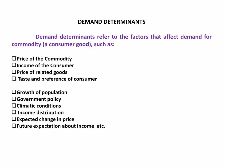
DEMAND DETERMINANTS

Demand determinants refer to the factors that affect demand forcommodity (a consumer good), such as:

Price of the CommodityIncome of the ConsumerPrice of related goods Taste and preference of consumer

Growth of populationGovernment policyClimatic conditions Income distributionExpected change in priceFuture expectation about income etc.

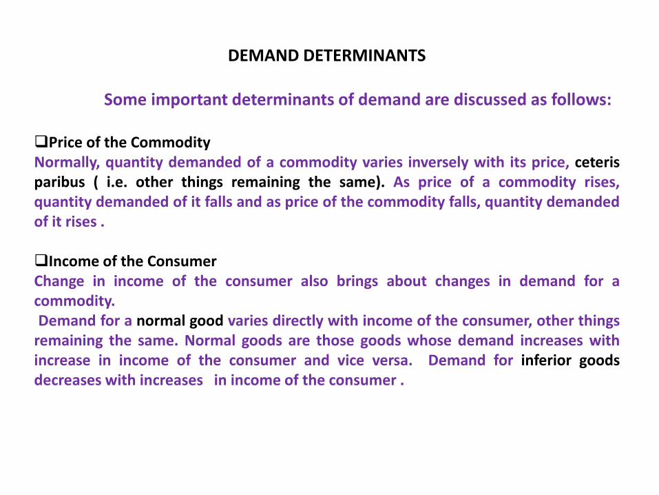
DEMAND DETERMINANTS

Some important determinants of demand are discussed as follows:

Price of the CommodityNormally, quantity demanded of a commodity varies inversely with its price, ceterisparibus ( i.e. other things remaining the same). As price of a commodity rises,quantity demanded of it falls and as price of the commodity falls, quantity demandedof it rises .

Income of the ConsumerChange in income of the consumer also brings about changes in demand for acommodity.Demand for a normal good varies directly with income of the consumer, other things

remaining the same. Normal goods are those goods whose demand increases withincrease in income of the consumer and vice versa. Demand for inferior goodsdecreases with increases in income of the consumer .

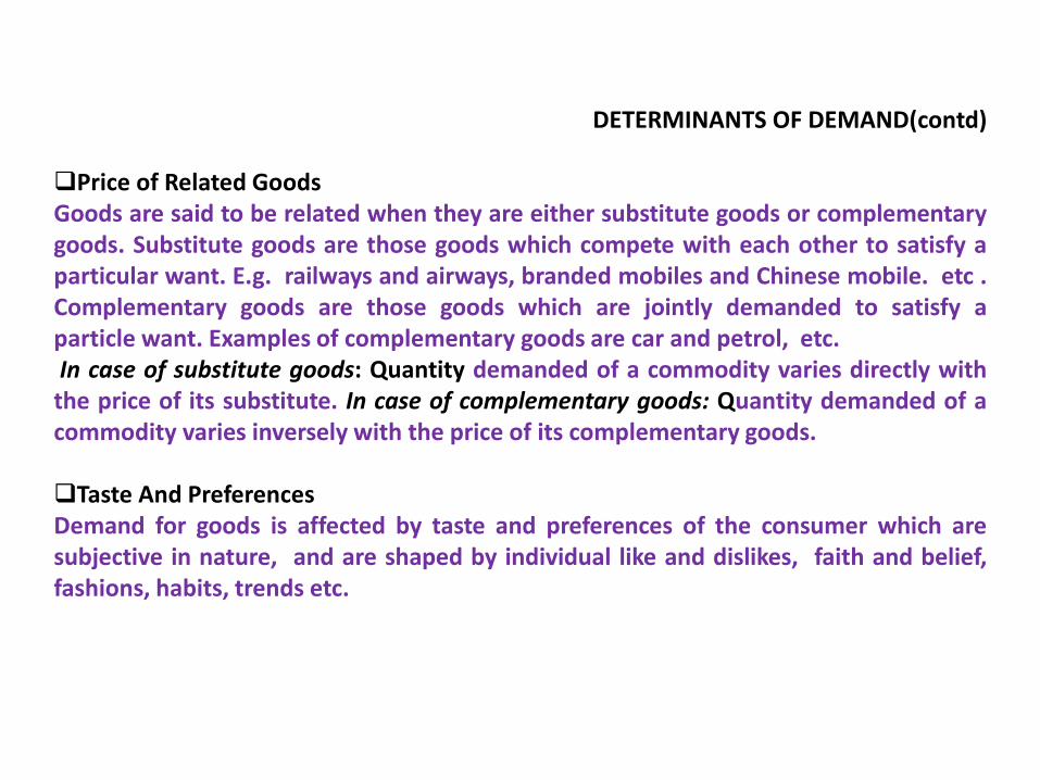
DETERMINANTS OF DEMAND(contd)

Price of Related GoodsGoods are said to be related when they are either substitute goods or complementarygoods. Substitute goods are those goods which compete with each other to satisfy aparticular want. E.g. railways and airways, branded mobiles and Chinese mobile. etc .Complementary goods are those goods which are jointly demanded to satisfy aparticle want. Examples of complementary goods are car and petrol, etc.In case of substitute goods: Quantity demanded of a commodity varies directly with

the price of its substitute. In case of complementary goods: Quantity demanded of acommodity varies inversely with the price of its complementary goods.

Taste And PreferencesDemand for goods is affected by taste and preferences of the consumer which aresubjective in nature, and are shaped by individual like and dislikes, faith and belief,fashions, habits, trends etc.

KINDS OF DEMAND

There are three kinds of demand relations which are usually studied under demand analysis such as: Price Demand, Income Demand and Cross Demand.

Price Demand: Price demand studies how demand for a commodity ( Dx) changes with respect to change in price(Px) , ceteris paribus (other things remaining the same). Dx= f (Px)

Income Demand: Income Demand examines how demand for commodity ( Dx) changes as a result of change in income of the consumer(Y) , other things remaining the same. Dx= f (Y)

Cross Demand: Cross demand studies how quantity demand of a commodity ( Dx) changes as a result of change in price of its related goods ( PR ), ceteris paribus . Cross demand function can be denoted as follows: Dx= f ( PR )

LAW OF DEMAND

The law of demand states that normally quantity demanded

of a commodity varies inversely with price, ceteris paribus.

In other words, the law of demand states that other things

reaming the same, lesser quantity of a commodity will be

demanded at higher prices, and more quantity of it will be

demanded at lower prices.

Demand Curve

0 Quantity demand

Price

D

D

Demand curve

Demand curve is the graphical representation of the relationship between demand for a commodity (Dx) and its price (Px) .

Normally, a demand curve slopes downwardfrom left to right indicating the operation of thelaw of demand.

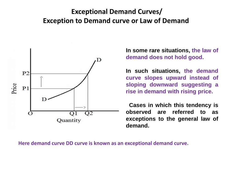
Here demand curve DD curve is known as an exceptional demand curve.

Exceptional Demand Curves/Exception to Demand curve or Law of Demand

In some rare situations, the law of

demand does not hold good.

In such situations, the demand

curve slopes upward instead of

sloping downward suggesting a

rise in demand with rising price.

Cases in which this tendency is

observed are referred to as

exceptions to the general law of

demand.

Exceptions to law of demand are

Giffen goods,

conspicuous consumption

conspicuous necessities,

expected changes in price,

extraordinary situations like natural disasters, famine, riots etc

Exceptional Demand Curves contd.

Giffen goods:

In case of certain inferior goods called Giffen goods, when the price falls, quite

often less quantity will be purchased than before because of the negative

income effect and people’s increasing preference for a superior commodity

with the rise in their real income. Few examples of giffen goods are cheap

potatoes, coarse cloth, coarse grain, etc.

Conspicuous consumption:

Some expensive commodities like diamonds, expensive cars, exorbitantly

high priced mobile phones etc., are used as status symbols to display one’s

wealth or , to distinguish oneself from average people. The more expensive

these commodities become, the higher their value as a status symbol and

hence, the greater the demand for them. Law of demand does not apply here.

Conspicuous necessities:

certain things become necessities of modern life. These are purchased even if

their prices rise. E.g. TV, refrigerators, mobile phones, automobiles.

Exception to Demand curve contd.

Expected Changes in Price:

Expected or anticipated changes in price of a commodity in future also can affect quantitydemanded of it at present. If it is expected that the price of a commodity will rise infuture, the demand for it rise and vice versa.

Extraordinary situations:

War, famines, riots, natural calamities are extra ordinary situations when

people’s behavior becomes abnormal. Law demand does not apply in

abnormal situations.

Exception to Demand curve contd.

ELASTICITY OF DEMAND

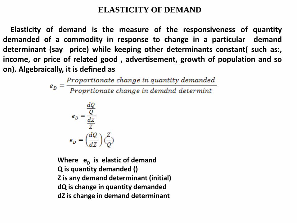
Elasticity of demand is the measure of the responsiveness of quantitydemanded of a commodity in response to change in a particular demanddeterminant (say price) while keeping other determinants constant( such as:,income, or price of related good , advertisement, growth of population and soon). Algebraically, it is defined as

Where eD is elastic of demandQ is quantity demanded ()Z is any demand determinant (initial)dQ is change in quantity demanded dZ is change in demand determinant

CONCEPTS OF ELASTICITY OF DEMAND

There may be as many as concepts of elasticity of demand as thenumber of demand determinants. Most important concepts ofelasticity of demand are:

Price elasticity of demand (here the demand determinant isprice of the commodity)

Income elasticity of demand (here the demand determinant isincome of consumer)

Cross elasticity of demand (here the demand determinant isprice of related goods)

PRICE ELASTICITY OF DEMAND

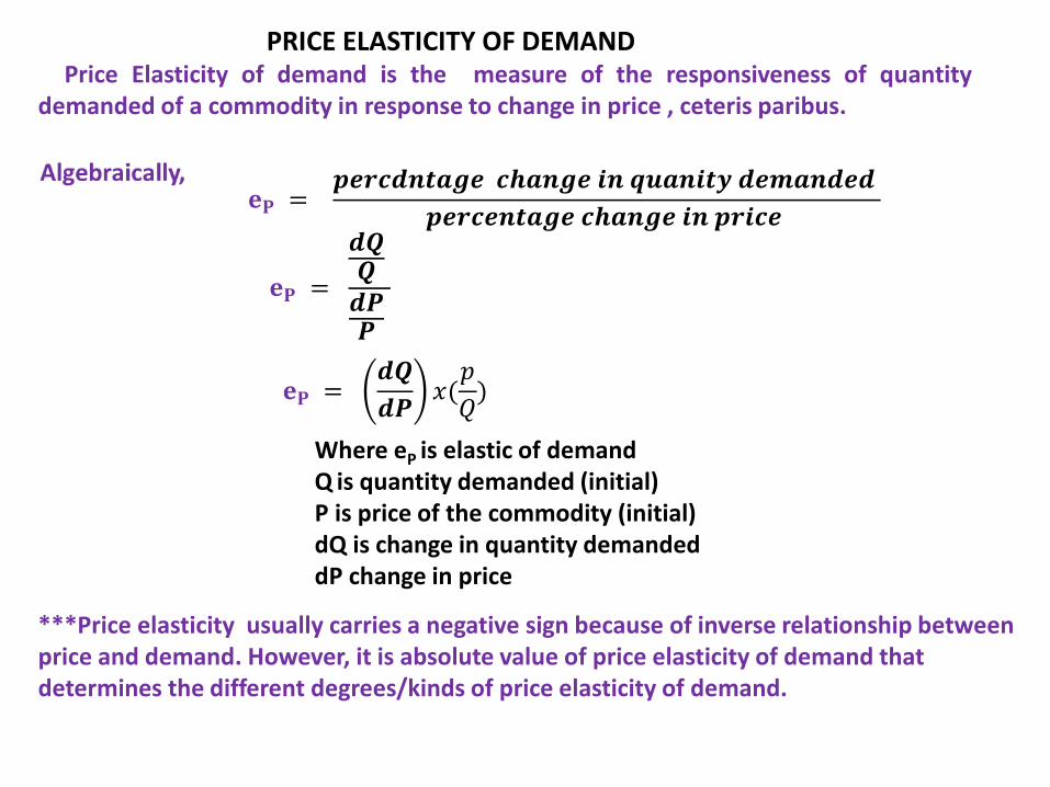
Where eP is elastic of demandQ is quantity demanded (initial)P is price of the commodity (initial)dQ is change in quantity demanded dP change in price

Price Elasticity of demand is the measure of the responsiveness of quantitydemanded of a commodity in response to change in price , ceteris paribus.

𝐞𝐏 =𝒑𝒆𝒓𝒄𝒅𝒏𝒕𝒂𝒈𝒆 𝒄𝒉𝒂𝒏𝒈𝒆 𝒊𝒏 𝒒𝒖𝒂𝒏𝒊𝒕𝒚 𝒅𝒆𝒎𝒂𝒏𝒅𝒆𝒅

𝒑𝒆𝒓𝒄𝒆𝒏𝒕𝒂𝒈𝒆 𝒄𝒉𝒂𝒏𝒈𝒆 𝒊𝒏 𝒑𝒓𝒊𝒄𝒆

𝐞𝐏 =

𝒅𝑸𝑸𝒅𝑷𝑷

𝐞𝐏 =𝒅𝑸

𝒅𝑷𝑥(𝑝

𝑄)

***Price elasticity usually carries a negative sign because of inverse relationship between price and demand. However, it is absolute value of price elasticity of demand that determines the different degrees/kinds of price elasticity of demand.

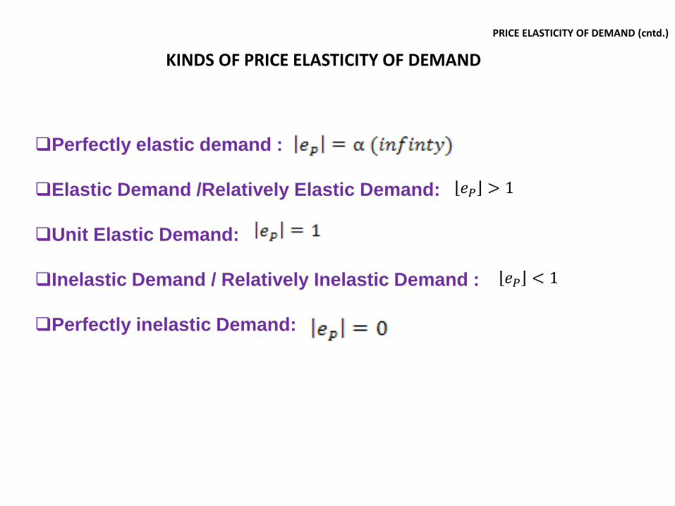
KINDS OF PRICE ELASTICITY OF DEMAND

Perfectly elastic demand :

Elastic Demand /Relatively Elastic Demand:

Unit Elastic Demand:

Inelastic Demand / Relatively Inelastic Demand :

Perfectly inelastic Demand:

PRICE ELASTICITY OF DEMAND (cntd.)

𝑒𝑃 > 1

𝑒𝑃 < 1

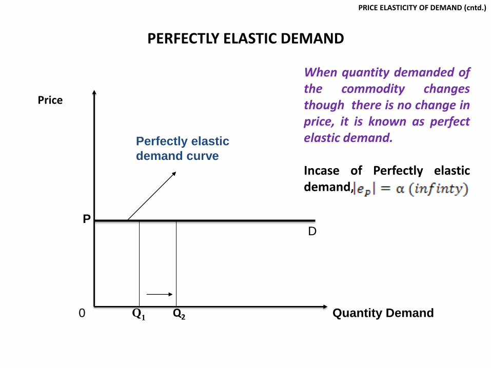
PERFECTLY ELASTIC DEMAND

Price

0 Quantity Demand

Perfectly elastic

demand curve

PD

When quantity demanded ofthe commodity changesthough there is no change inprice, it is known as perfectelastic demand.

Incase of Perfectly elasticdemand,

PRICE ELASTICITY OF DEMAND (cntd.)

Q1Q2

ELASTIC DEMAND

Elastic demand curve

0 Quantity demanded

Price

D

D

When the proportionatechange in demand is morethan the proportionatechanges in price, it is knownas relatively elastic demand.E.g. luxury goods

Incase of elastic demand,

PRICE ELASTICITY OF DEMAND (cntd.)

Q1Q2

P2

P1

𝑒𝑃 > 1

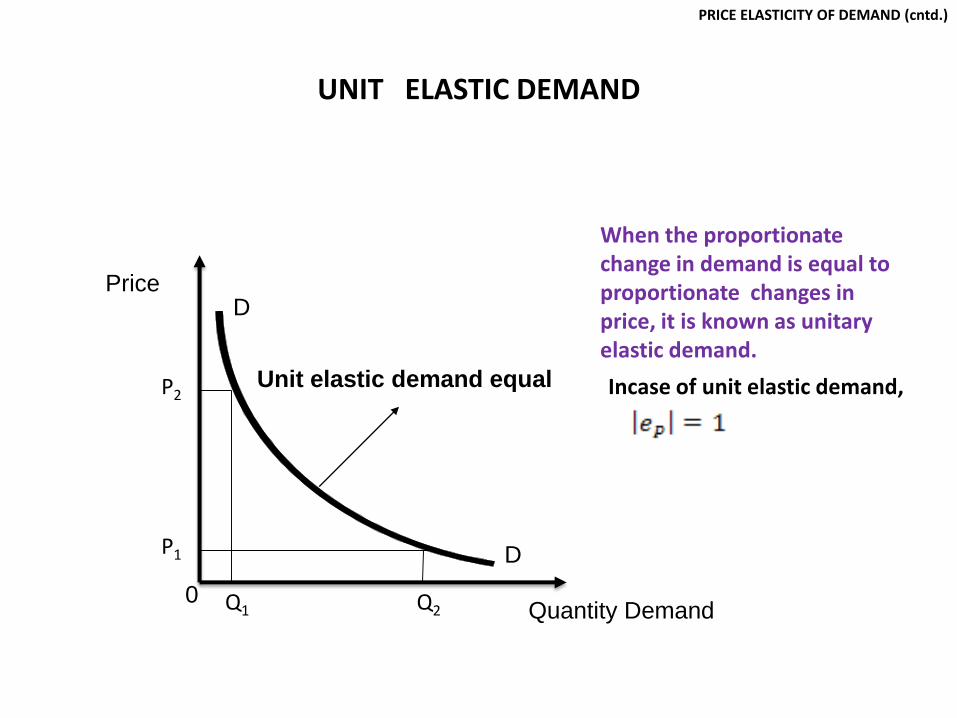
UNIT ELASTIC DEMAND

Unit elastic demand equal

0Quantity Demand

Price D

D

When the proportionate change in demand is equal to proportionate changes in price, it is known as unitary elastic demand.

Incase of unit elastic demand,

PRICE ELASTICITY OF DEMAND (cntd.)

P2

P1

Q1 Q2

INELASTIC DEMAND

Inelastic demand curve

Quantity Demanded O

PriceD

D

When theproportionate changein demand is less thanthe proportionatechanges in price, it isknown as relativelyinelastic demand. e.g.necessities, electricityetc.

Incase of inelastic demand,

PRICE ELASTICITY OF DEMAND (cntd.)

P2

Q2Q1

P1

𝑒𝑃 < 1

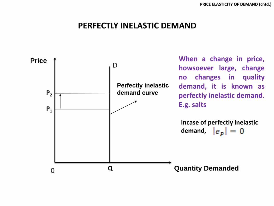
PERFECTLY INELASTIC DEMAND

D

Perfectly inelastic

demand curve

0

Price

Quantity Demanded

When a change in price,howsoever large, changeno changes in qualitydemand, it is known asperfectly inelastic demand.E.g. salts

Incase of perfectly inelasticdemand,

PRICE ELASTICITY OF DEMAND (cntd.)

P1

P2

Q

Income Elasticity Of Demand

Income Elasticity of demand is the measure of the responsiveness of quantitydemanded of a commodity in response to change in income of the consumer, ceterisparibus.

or,

or,

,

is income elasticity of demand Q is the quantity demanded (initial)Y is the income of the consumer (initial)dQ is the change in quantity demanded dY is the change in income

Where

𝐞𝒀 =𝒑𝒆𝒓𝒄𝒅𝒏𝒕𝒂𝒈𝒆 𝒄𝒉𝒂𝒏𝒈𝒆 𝒊𝒏 𝒒𝒖𝒂𝒏𝒊𝒕𝒚 𝒅𝒆𝒎𝒂𝒏𝒅𝒆𝒅

𝒑𝒆𝒓𝒄𝒆𝒏𝒕𝒂𝒈𝒆 𝒄𝒉𝒂𝒏𝒈𝒆 𝒊𝒏 𝒊𝒏𝒄𝒐𝒎𝒆 𝒐𝒇 𝒄𝒐𝒎𝒖𝒔𝒎𝒆𝒓

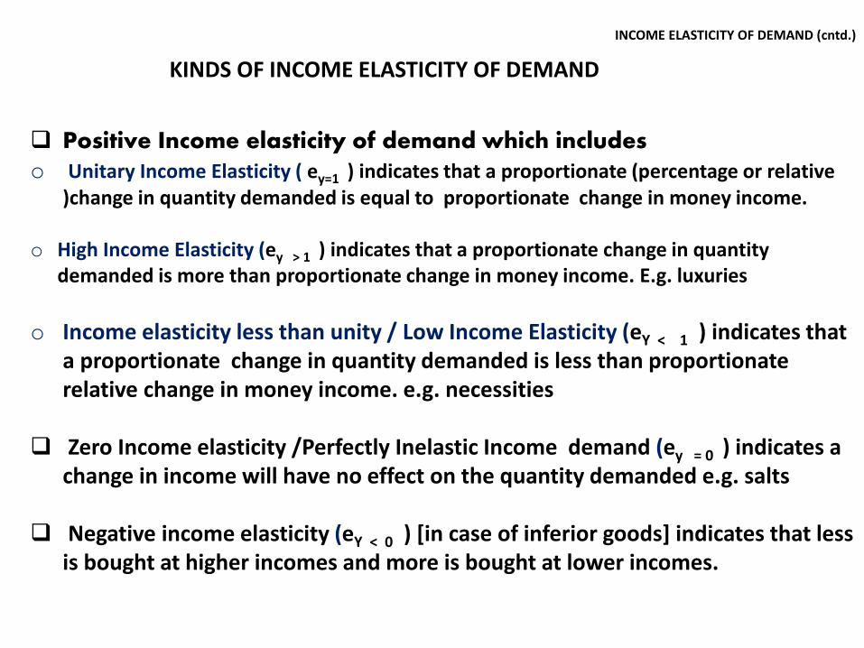
KINDS OF INCOME ELASTICITY OF DEMAND

Positive Income elasticity of demand which includes o Unitary Income Elasticity ( ey=1 ) indicates that a proportionate (percentage or relative

)change in quantity demanded is equal to proportionate change in money income.

o High Income Elasticity (ey > 1 ) indicates that a proportionate change in quantity demanded is more than proportionate change in money income. E.g. luxuries

o Income elasticity less than unity / Low Income Elasticity (eY < 1 ) indicates that a proportionate change in quantity demanded is less than proportionate relative change in money income. e.g. necessities

Zero Income elasticity /Perfectly Inelastic Income demand (ey = 0 ) indicates achange in income will have no effect on the quantity demanded e.g. salts

Negative income elasticity (eY < 0 ) [in case of inferior goods] indicates that less is bought at higher incomes and more is bought at lower incomes.

INCOME ELASTICITY OF DEMAND (cntd.)

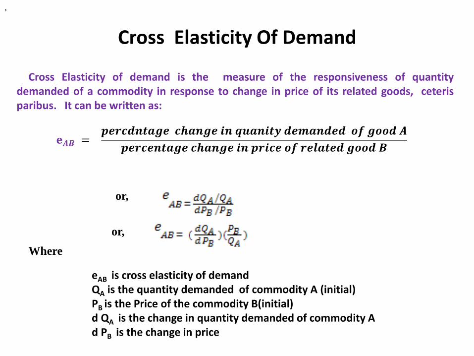
Cross Elasticity Of Demand

Cross Elasticity of demand is the measure of the responsiveness of quantitydemanded of a commodity in response to change in price of its related goods, ceterisparibus. It can be written as:

or,

or,

,

eAB is cross elasticity of demand QA is the quantity demanded of commodity A (initial)PB is the Price of the commodity B(initial)d QA is the change in quantity demanded of commodity Ad PB is the change in price

Where

𝐞𝑨𝑩 =𝒑𝒆𝒓𝒄𝒅𝒏𝒕𝒂𝒈𝒆 𝒄𝒉𝒂𝒏𝒈𝒆 𝒊𝒏 𝒒𝒖𝒂𝒏𝒊𝒕𝒚 𝒅𝒆𝒎𝒂𝒏𝒅𝒆𝒅 𝒐𝒇 𝒈𝒐𝒐𝒅 𝑨

𝒑𝒆𝒓𝒄𝒆𝒏𝒕𝒂𝒈𝒆 𝒄𝒉𝒂𝒏𝒈𝒆 𝒊𝒏 𝒑𝒓𝒊𝒄𝒆 𝒐𝒇 𝒓𝒆𝒍𝒂𝒕𝒆𝒅 𝒈𝒐𝒐𝒅 𝑩

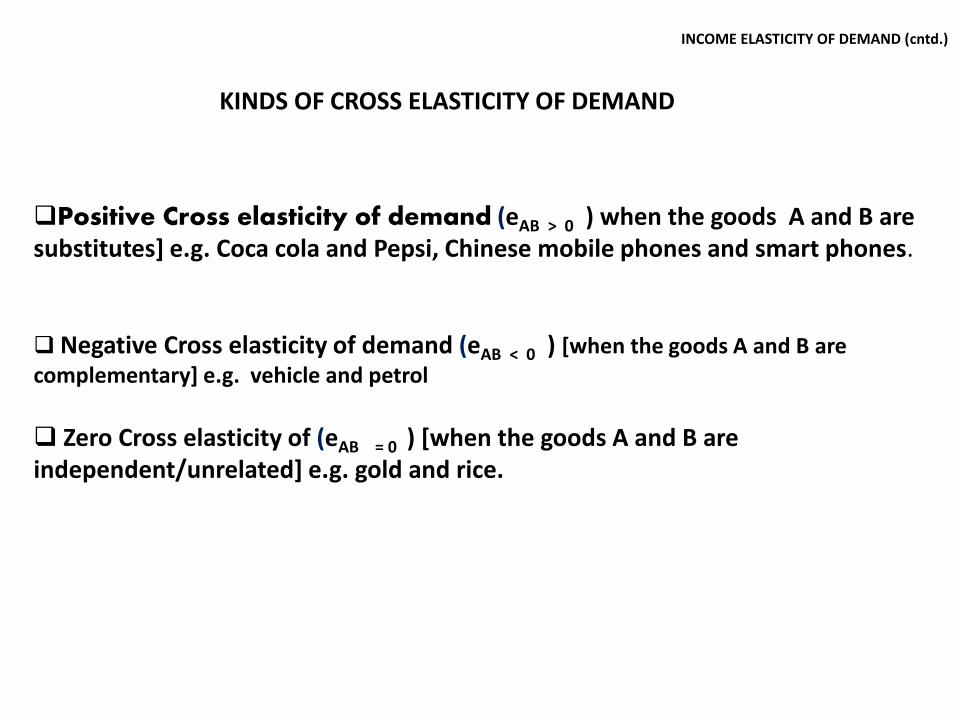
KINDS OF CROSS ELASTICITY OF DEMAND

Positive Cross elasticity of demand (eAB > 0 ) when the goods A and B are substitutes] e.g. Coca cola and Pepsi, Chinese mobile phones and smart phones.

Negative Cross elasticity of demand (eAB < 0 ) [when the goods A and B are complementary] e.g. vehicle and petrol

Zero Cross elasticity of (eAB = 0 ) [when the goods A and B are independent/unrelated] e.g. gold and rice.

INCOME ELASTICITY OF DEMAND (cntd.)

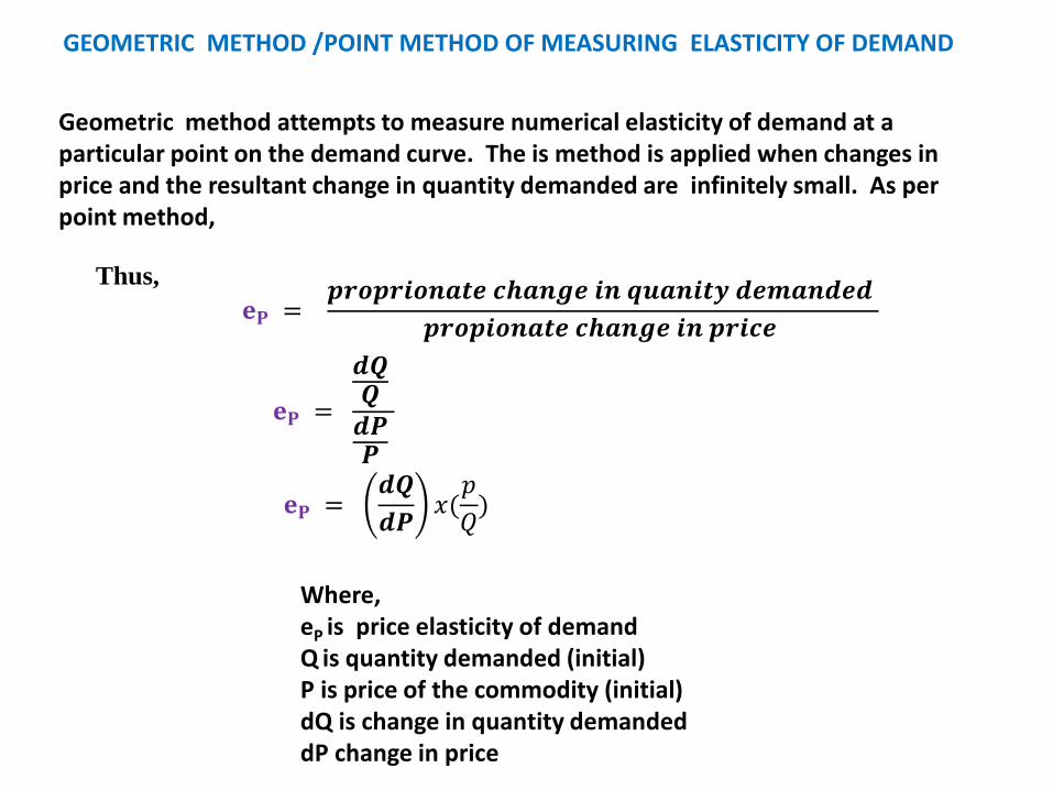
GEOMETRIC METHOD /POINT METHOD OF MEASURING ELASTICITY OF DEMAND

Where, eP is price elasticity of demandQ is quantity demanded (initial)P is price of the commodity (initial)dQ is change in quantity demanded dP change in price

Geometric method attempts to measure numerical elasticity of demand at a particular point on the demand curve. The is method is applied when changes in price and the resultant change in quantity demanded are infinitely small. As per point method,

𝐞𝐏 =𝒑𝒓𝒐𝒑𝒓𝒊𝒐𝒏𝒂𝒕𝒆 𝒄𝒉𝒂𝒏𝒈𝒆 𝒊𝒏 𝒒𝒖𝒂𝒏𝒊𝒕𝒚 𝒅𝒆𝒎𝒂𝒏𝒅𝒆𝒅

𝒑𝒓𝒐𝒑𝒊𝒐𝒏𝒂𝒕𝒆 𝒄𝒉𝒂𝒏𝒈𝒆 𝒊𝒏 𝒑𝒓𝒊𝒄𝒆

Thus,

𝐞𝐏 =

𝒅𝑸𝑸𝒅𝑷𝑷

𝐞𝐏 =𝒅𝑸

𝒅𝑷𝑥(𝑝

𝑄)

O

Price

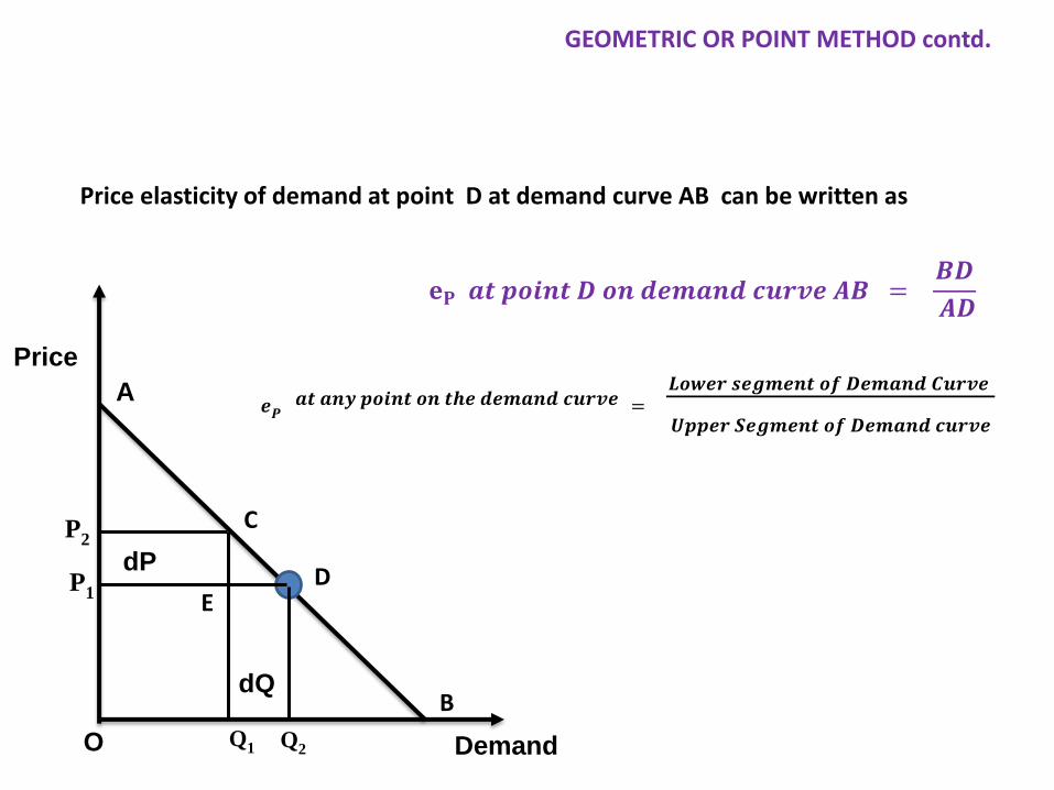
GEOMETRIC OR POINT METHOD contd.

A

B

Demand

D

𝐞𝐏 𝒂𝒕 𝒑𝒐𝒊𝒏𝒕 𝑫 𝒐𝒏 𝒅𝒆𝒎𝒂𝒏𝒅 𝒄𝒖𝒓𝒗𝒆 𝑨𝑩 =𝑩𝑫

𝑨𝑫

dP

dQ

P1

P2

Q1 Q2

C

E

Price elasticity of demand at point D at demand curve AB can be written as

𝒆𝑷𝒂𝒕 𝒂𝒏𝒚 𝒑𝒐𝒊𝒏𝒕 𝒐𝒏 𝒕𝒉𝒆 𝒅𝒆𝒎𝒂𝒏𝒅 𝒄𝒖𝒓𝒗𝒆 =

𝑳𝒐𝒘𝒆𝒓 𝒔𝒆𝒈𝒎𝒆𝒏𝒕 𝒐𝒇 𝑫𝒆𝒎𝒂𝒏𝒅 𝑪𝒖𝒓𝒗𝒆

𝑼𝒑𝒑𝒆𝒓 𝑺𝒆𝒈𝒎𝒆𝒏𝒕 𝒐𝒇 𝑫𝒆𝒎𝒂𝒏𝒅 𝒄𝒖𝒓𝒗𝒆

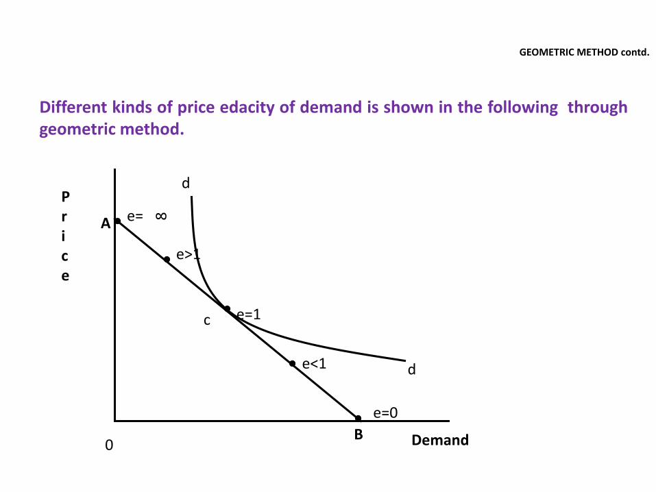
GEOMETRIC METHOD contd.

Different kinds of price edacity of demand is shown in the following throughgeometric method.

B

A

c

d

d

0 Demand

Price

e=1

e= 8

e>1

e<1

e=0

Utility is defined as the power of commodity to satisfy a human want.

People know utility of goods by means of introspection and therefore issubjective.

Being subjective, it varies from persons to persons. That is, different personsmay derive different amount of utility/satisfaction from the same good.

The desire for a commodity by a person depends upon the utility he expectsto obtain from it.

UTILITY

Total UtilityTotal psychological satisfaction obtained by a consumer from consuming a given amountof a particular commodity is called total utility.

Marginal UtilityMarginal Utility is the extra utility derived by a consumer from the consumption of anadditional unit of a particular commodity.

TOTAL UTILITY AND MARGINAL UTILITY

RELATIONSHIP BETWEEN TU AND MU

-5

0

5

10

15

20

25

30

35

1 2 3 4 5 6 7

To

tal/M

arg

ina

l U

tiliti

es

Quantity of Commodity

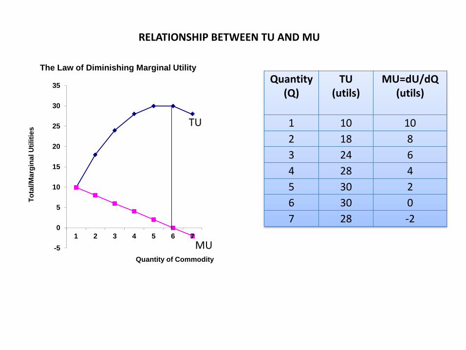
The Law of Diminishing Marginal Utility

TU

MU

Quantity(Q)

TU(utils)

MU=dU/dQ(utils)

1 10 10

2 18 8

3 24 6

4 28 4

5 30 2

6 30 0

7 28 -2

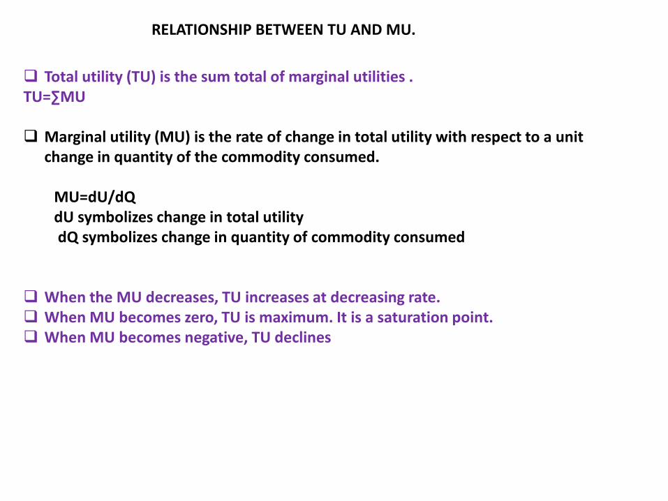
Total utility (TU) is the sum total of marginal utilities .TU=∑MU

Marginal utility (MU) is the rate of change in total utility with respect to a unit change in quantity of the commodity consumed.

MU=dU/dQdU symbolizes change in total utility dQ symbolizes change in quantity of commodity consumed

When the MU decreases, TU increases at decreasing rate. When MU becomes zero, TU is maximum. It is a saturation point. When MU becomes negative, TU declines

RELATIONSHIP BETWEEN TU AND MU.

Laws of Diminishing Marginal Utility

Law of Equi-Marginal Utility

LAWS OF CARDINAL UTILITY ANALYSIS

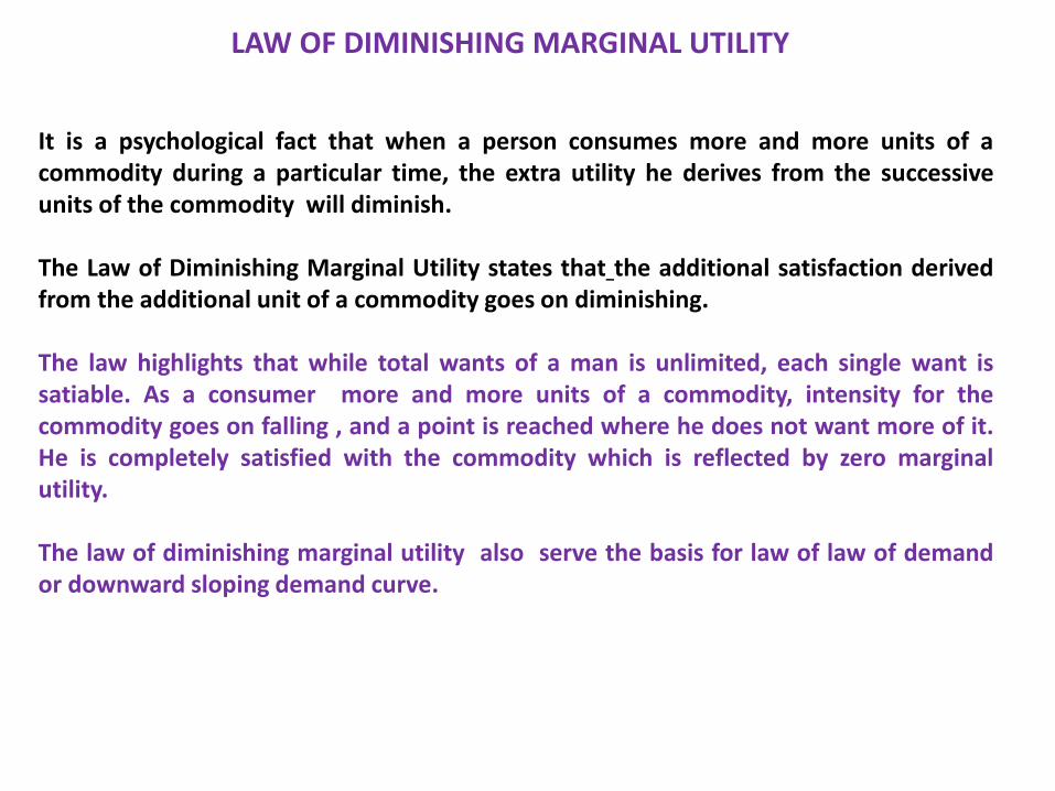
It is a psychological fact that when a person consumes more and more units of acommodity during a particular time, the extra utility he derives from the successiveunits of the commodity will diminish.

The Law of Diminishing Marginal Utility states that the additional satisfaction derivedfrom the additional unit of a commodity goes on diminishing.

The law highlights that while total wants of a man is unlimited, each single want issatiable. As a consumer more and more units of a commodity, intensity for thecommodity goes on falling , and a point is reached where he does not want more of it.He is completely satisfied with the commodity which is reflected by zero marginalutility.

The law of diminishing marginal utility also serve the basis for law of law of demandor downward sloping demand curve.

LAW OF DIMINISHING MARGINAL UTILITY

A consumer is in equilibrium when he maximises his utility or satisfaction by

spending his given money income on different goods.

Consumer’s Equilibrium in Case of Single Good

Let us take a simple model of single commodity X.

The consumer either spends his money income on the good or retains his money income.

In such situation, the consumer will be in equilibrium when MUX = PX

Where, MUX is marginal utility of commodity X

PX is price of the commodity X.

If MUX > PX , the consumer can increase his well-being by purchasing more units of the

commodity X.

If MUX < PX , the consumer can increase his total cost satisfaction by cutting down the

quantity of commodity X and keeping more of his income unspent.

Thus, he maximises his satisfaction when MUX = PX

CONSUMER’S EQUILIBRIUM

CONSUMER’S EQUILIBRIUM contd.

Consumer’s Equilibrium In case of More Than One Good and

Law of Equi-Marginal Utility

The law of equi-marginal utility states that a consumer distributes his limited

income among various commodities in such a way that marginal utility of money

expenditure on each good is equal. This is the condition of consumer’s equilibrium in

case of more than one commodity.

Marginal utility of money expenditure on a good is the ratio of marginal utility

of the commodity to price of it.

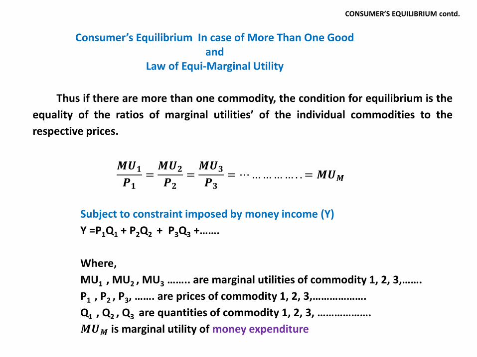
CONSUMER’S EQUILIBRIUM contd.

Consumer’s Equilibrium In case of More Than One Good and

Law of Equi-Marginal Utility

Thus if there are more than one commodity, the condition for equilibrium is the

equality of the ratios of marginal utilities’ of the individual commodities to the

respective prices.

𝑴𝑼𝟏

𝑷𝟏=𝑴𝑼𝟐

𝑷𝟐=𝑴𝑼𝟑

𝑷𝟑= ⋯………… . . = 𝑴𝑼𝑴

Subject to constraint imposed by money income (Y)

Y =P1Q1 + P2Q2 + P3Q3 +…….

Where,

MU1 , MU2 , MU3 …….. are marginal utilities of commodity 1, 2, 3,…….

P1 , P2 , P3, ……. are prices of commodity 1, 2, 3,……………….

Q1 , Q2 , Q3 are quantities of commodity 1, 2, 3, ……………….

𝑴𝑼𝑴 is marginal utility of money expenditure

SUPPLY

Supply indicates quantities of a commodity of a offered for sale at each possible

price at a given time period, other things constant

Determinants of Supply

Price of the product

State of technology

Prices of relevant resources

Prices of alternative goods

Producer expectations

Number of producers/sellers in the market

LAW OF SUPPLY

Law of supply states that normally, the quantity supplied varies directly with its

price, other things constant.

In other words , law of supply states that lower the price, the smaller the

quantity supplied and higher the price, the greater the quantity supplied.

Supply Curve

0 Supply

Price

S

S

Supply Curve

Supply curve is the graphical representation of the relationship between supply of a commodity (Dx) and its price (Px) .

Normally, a supply curve slopes upward from leftto right indicating the operation of the law ofsupply.

0

E

S(P)

D(P)

Surplus

Price

Demand/Supply Demand=

Supply

Shortage

EQUILIBRIUM PRICE Equilibrium price acommodity is determinedat point(E) where marketdemand is equal tomarket supply.

At price P2 , supply ismore demand and thusthere is surplus in themarket. Price will fallcausing supply to fall anddemand to rise. Pricewill continue to fall untilit reaches equilibriumprice Pe at whichDemand=Supply (Equilibrium point E).

P2

P1

Q1 Q2 Qe

At P1, demand is more than supply and as such there is shortage in the market. Pricewill raise causing demand to fall and supply to rise. Price will continue to rise until itreaches equilibrium price at which Demand=Supply ( Equilibrium point E).

Pe