deliverable d1.2 power system analysis and key … · report page 2 of 206 disclaimer the...
TRANSCRIPT

REPORT
Page 1 of 206
............................................................................................................................................................
Acronym: MIGRATE – Massive InteGRATion of power Electronic devices
Grant Agreement Number: 691800
Horizon 2020 – LCE-6: Transmission Grid and Wholesale Market
Funding Scheme: Collaborative Project
............................................................................................................................................................
Deliverable D1.2
Power System Analysis and Key
Performance Indicators
Date: 31.01.2018
Contact: [email protected]

REPORT
Page 2 of 206
Disclaimer The information, documentation and figures in this deliverable are written by the MIGRATE project
consortium under EC grant agreement No 691800 and do not necessarily reflect the views of the European Commission. The European Commission is not liable for any use that may be made of the information contained herein.
Dissemination level:
Public
Restricted to other programme participants (including the Commission Services)
Restricted to bodies determined by the MIGRATE project
Confidential to MIGRATE project and Commission Services X

REPORT
Page 3 of 206
Document info sheet Document name: Power System Analysis Approaches and Key Performance Indicators
Responsible partner: TUD1
WP: 1
Task: 1.2/1.4
Deliverable number: 1.2
Revision: 2.0
Revision date: 31.01.2018
Name Company Name Company
Authors:
J.L. Rueda Torres
E. Rakhshani
D. Wang
B. Tuinema
N. Farrokhseresht
D. Gusain
A. Perilla
J. Mola Jimenez
V. Sewdien
S. Rüberg
TUD
TUD
TUD
TUD
TUD
TUD
TUD
TUD
TenneT2
TenneT3
T. Breithaupt
D. Herwig
F. Goudarzi
A. Pawellek
A. Neufeld
R. Meyer
L. Hofmann
A. Mertens
M. Val Escudero
J. Kilter
LUH4
LUH
LUH
LUH
LUH
LUH
LUH
LUH
EirGrid5
Elering6
Task leader: J.L. Rueda Torres TUD
WP leader: S. Rüberg TenneT
Revision history log
Revision Date of release Author Summary of
changes
0.0 – Draft 30.06.2017 TUD, LUH,
TenneT, EirGrid Initial draft
1.0 – Draft 03.10.2017 TUD, LUH,
TenneT, EirGrid First complete draft
2.0 31.01.2018 TUD, LUH,
TenneT, EirGrid
Comments from T1.2/T1.4 partners
are addressed
1 Delft University of Technology, The Netherlands 2 TenneT TSO B.V., The Netherlands 3 TenneT TSO GmbH, Germany 4 Leibniz Universität Hannover, Germany 5 EirGrid, Ireland 6 Elering, Estonia

REPORT
Page 4 of 206
Executive Summary
This Deliverable is devoted to the study of four model problems, which describe the modelling and
simulation needs to enable a suitable (i.e. accurate) recreation of a given stability phenomenon
when the studied system is close to or in an unstable condition. The model problems are defined
based on the top ranked stability issues listed in Deliverable D1.1 (‘Report on Systemic Issues’).
These issues were evaluated by Transmission System Operators (TSOs) of the MIGRATE
consortium and other members of the European Network of Transmission System Operators for
Electricity (ENTSO-E). Among the model problems are the frequency performance within the
inertial response time window of the frequency containment period, large-disturbance rotor angle
stability, small-disturbance voltage stability, and sub-synchronous controller interactions.
Chapter 1 revises the main findings from deliverable D1.1 and outlines the scope of the work
carried out in tasks T1.2 (‘Power system analysis approaches and development of KPIs to measure
the distance to instability’) and T1.4 (‘Development and use of a small set of generic test cases
able to grasp system stability issues raised by the growing PE connection into any control zone’). In
Chapter 2, the current state-of-the-art modelling in power systems and the capabilities of Power
Electronics-Interfaced Generation (PEIG) is revised and discussed. At the end of this chapter, a
manufacturer survey about expected future capabilities of Power Electronic (PE) converters with
respect to the grid codes is discussed. It is pointed out that the technical feasibility of many non-
exhaustive requirements depends on the concrete specifications demanded by the relevant TSO,
which is of significant importance for requirements that may demand an energy storage. The
overall consent of the interviewed manufacturers was that the benefit of each requirement for a
particular grid application has to be weighed against the cost of implementation and testing.
The development of a set of generic test cases and the implementation of transition scenarios in
the Great Britain and Irish systems are presented in Chapter 3. Three generic test cases are
introduced. The generic test cases are based on existing benchmark systems for power system
stability studies available in literature. These benchmark systems were modified to account for high
penetration levels of wind power generation and to evaluate the impacts on the stability
performance due to the decrease of the number of conventional power plants connected to the grid.
The first generic test case is used in Chapter 4 to study the frequency performance, considering the
inertial response time window (1-30 seconds from the time of occurrence of an imbalance),
whereas the second one is used to study the large-disturbance rotor angle stability and the small-
disturbance voltage stability. The third generic test case is used to study sub-synchronous
controller interactions. This chapter also shows a simple methodology to exploit information from
power system planning to create different transition scenarios, which constitute different topologies
and entail different composition of generation and demand for future situations of a power system
that undergoes a dramatic transformation from synchronous generation dominated behaviour to
PEIG dominated behaviour. The methodology is applied to the Great Britain system, which is used

REPORT
Page 5 of 206
together with the model of the Irish system for testing the Key Performance Indicators (KPIs)
proposed in Chapter 4.
In Chapter 4, the notion of KPI is introduced. Here, a KPI constitutes a way to map the values of a
system variable or set of system variables (e.g. kinetic energy) onto the actual value of a stability
indicator (e.g. frequency nadir), thus allowing to estimate the distance to instability. The distance
to instability is an indication of the stability status of the system and how the system will move
from stable status to the stability limit (i.e. threshold defined by the operator for the stability
indicator) as a consequence of changes in the key variables. Methods to determine the KPIs based
on offline simulations are proposed. DIgSILENT PowerFactory and PSCAD are used to perform RMS
simulations and EMT simulations, respectively. Widely used indicators for the assessment of the
frequency performance within the inertial response time window of the frequency containment
period, and the assessment of the large-disturbance rotor angle stability are integrated into the
proposed KPIs for these phenomena, whereas new indicators are proposed and integrated into the
KPIs for small-disturbance voltage stability and sub-synchronous controller interactions. Numerical
results obtained by using the generic test cases provide insight into the stability performance of
systems with high penetration levels of PEIG, whereas the tests conducted by using the Great
Britain system (further assessment of frequency performance in the frequency containment period,
large-disturbance rotor angle stability, and small-disturbance voltage stability) and the Irish
system (additional case study concerning frequency performance in the frequency containment
period) shed light into the feasibility and effectiveness of the proposed KPIs when applied to larger
size systems. This chapter also provides recommendations for future studies and application of the
KPIs in power system operation.

REPORT
Page 6 of 206
Contents
Executive Summary .................................................................................... 4
Contents ................................................................................................... 6
List of Figures ............................................................................................ 9
List of Tables ........................................................................................... 14
Abbreviations ........................................................................................... 16
1 Introduction ....................................................................................... 19
1.1 Motivation ................................................................................... 19
1.2 Deliverable 1.2 in the Context of MIGRATE and WP1 ........................ 19
1.3 Main Findings from Deliverable 1.1 ................................................ 20
1.4 Scope, Objectives and Approach of Tasks 1.2 and 1.4 ...................... 22
1.5 Outline of Deliverable 1.2 ............................................................. 23
2 State-of-the-Art Power System Modelling and Simulation ......................... 24
2.1 Introduction ................................................................................ 24
2.2 Power System Modelling ............................................................... 24
2.3 Power System Simulation Practices ................................................ 27
2.3.1 Simulation of Power System Dynamic Response .................... 27
2.3.2 Review on Current TSO Practices ........................................ 28
2.4 Manufacturer Review of PE Capabilities and Network Codes............... 30
2.5 Conclusions ................................................................................. 37
3 Modelling of Transmission Systems with high Penetration of PE Devices ..... 39
3.1 Introduction ................................................................................ 39
3.2 Development of Generic Test Cases ............................................... 39
3.2.1 General Description of Generic Test Cases ............................ 39

REPORT
Page 7 of 206
3.2.2 Power System Modelling in RMS and EMT ............................. 40
3.2.3 Generic Test Case 1: Frequency Performance in the Frequency
Containment Period ........................................................... 53
3.2.4 Generic Test Case 2: Large-Disturbance Rotor Angle Stability
and Small-Disturbance Voltage Stability ............................... 56
3.2.5 Generic Test Case 3: Sub-synchronous Controller Interactions 59
3.3 Development of Realistic Test Cases of Medium Size ........................ 60
3.3.1 Development of Transition Scenarios ................................... 60
3.3.2 Implementation into the GB Test System ............................. 63
3.3.3 Implementation into the Irish Test System ........................... 72
4 Study of Power System Stability ........................................................... 81
4.1 Introduction ................................................................................ 81
4.2 KPI for Assessment of Frequency Performance ................................ 82
4.2.1 Frequency Performance in Containment Period ..................... 83
4.2.2 Analysis of ROCOF and NADIR using Generic Test Case 1 ....... 86
4.2.3 Proposition of KPI for Assessment of Frequency Performance 102
4.2.4 Recommendations and Usage in Control Room ................... 111
4.2.5 Validation with the Irish System ....................................... 113
4.3 KPI for Large-Disturbance Rotor Angle Stability ............................. 120
4.3.1 Introduction ................................................................... 120
4.3.2 Decision Trees Background ............................................... 122
4.3.3 Background of MVMO ...................................................... 125
4.3.4 Outline of the Proposed Method of Selecting Key Variables ... 125
4.3.5 Test Results with Generic Test Case 2 ................................ 128
4.3.6 Test Results on the GB System ......................................... 135
4.3.7 Conclusions and Recommendations ................................... 141
4.4 KPI for Small-Disturbance Voltage Stability ................................... 143
4.4.1 Introduction ................................................................... 143
4.4.2 Definitions ...................................................................... 144

REPORT
Page 8 of 206
4.4.3 Proposed Indicator: Calculation Procedure .......................... 149
4.4.4 Results for Generic Test Case 2......................................... 151
4.4.5 Validation on the GB Power System ................................... 154
4.4.6 Conclusions and Recommendations ................................... 156
4.5 KPI for Sub-Synchronous Controller Interactions ........................... 158
4.5.1 Introduction ................................................................... 158
4.5.2 Assumptions ................................................................... 159
4.5.3 Definitions ...................................................................... 160
4.5.4 Calculation Procedure ...................................................... 162
4.5.5 Results for different Case Studies ...................................... 169
4.5.6 Conclusions and Recommendations ................................... 174
4.5.7 Control Room Implementation .......................................... 175
A Generic Test Cases ............................................................................ 176
B Transition Scenario Implementation .................................................... 183
B.1 Implementation into the GB Test System ...................................... 183
B.2 Implementation into the Irish Test System ................................... 188
C Assessment of KPIs in the Irish System – Supplementary Information ..... 194
C.1 Generation Dispatches – WINTER PEAK ........................................ 194
C.2 Generation Dispatches – SUMMER PEAK ....................................... 196
D Use of Inertia for Frequency Stability KPI ............................................. 198
Bibliography .......................................................................................... 199
REPORT
Page 9 of 206
List of Figures
Figure 2.1 Classification of transients according to their classical time frame t, their
eigenvalue groups 𝜆 and their expansion [8]. ......................................................... 26
Figure 2.2 Phenomena time scales in electric power systems [11]. ........................................... 26
Figure 3.1 Overview of the model problem. ........................................................................... 40
Figure 3.2 General example of the DSL components implementation. ....................................... 42
Figure 3.3 Controller structure of the wind turbine model in PowerFactory. ............................... 44
Figure 3.4 External data file selection of wind turbines in PowerFactory. ................................... 45
Figure 3.5 Interface for the connection of the wind model to the grid. ...................................... 45
Figure 3.6 Structure of WP controller proposed by IEC 61400-27-1. ......................................... 46
Figure 3.7 Grid interface of a wind park with two types of wind turbines. ................................. 47
Figure 3.8 Performance of active power injected into the grid for the wind turbine models (WT
type 4 in red and WT type 3 in green) in the GB test system. ................................... 47
Figure 3.9 Single 3.6 MW DFIG connected to an equivalent voltage source through a 50x unit
multiplier. .......................................................................................................... 49
Figure 3.10 Electrical structure of DFIG electromechanical system. ............................... 50
Figure 3.11 (a) initialisation of Detailed DFIG Model and (b) detailed DFIG Response
to 150 ms 3-phase SC at the PCC. ........................................................................ 51
Figure 3.12 Overview of the external network connection. ........................................... 51
Figure 3.13 Overview of the type-4 wind turbine module. ............................................ 52
Figure 3.14 Initialisation of Detailed Type 4 Model. ..................................................... 52
Figure 3.15 Modified PST16 benchmark system. ......................................................... 53
Figure 3.16 Simplified overview load dispatch scenarios (modified PST16 system). ......... 55
Figure 3.17 Modified generic test case 2. ................................................................... 57
Figure 3.18 Modified IEEE 9 Bus System – Single Line Diagram. ................................... 58
Figure 3.19 Generic Test Case SSCI – Single Line Diagram. ......................................... 59
Figure 3.20 Extended Model for SSCI – Single Line Diagram. ....................................... 60
Figure 3.21 The S-curve model of transitions. ............................................................ 61
Figure 3.22 Great Britain reduced transmission system (from [49] - Figure 3.1, pp.
74). ........................................................................................................... 64
Figure 3.23 Overview of matching process with the work flow. ..................................... 65
Figure 3.24 Mapping of the 5 ETYS regions onto the 29 zone network model. ................. 65
Figure 3.25 Steps to relate the National Grid information with the existing reduced GB
model. ........................................................................................................... 66
Figure 3.26 Development of conventional generation and PEIG (Gone Green & No
Progression). ..................................................................................................... 67
Figure 3.27 Node bus structure in the reduced GB system (from [49] - Figure 3.2, pp.
76). ........................................................................................................... 69
Figure 3.28 PowerFactory Data manager with the 9 transition scenarios archives. ........... 69
Figure 3.29 Procedure to create transition scenarios in the GB system. .......................... 70

REPORT
Page 10 of 206
Figure 3.30 Connection of offshore wind park to the grid. ............................................ 71
Figure 3.31 Connection of onshore wind park to the grid. ............................................ 71
Figure 3.32 Connection of synchronous generators to the grid in all scenarios. ............... 72
Figure 3.33 All Island Transmission System (July 2016) [55]. ...................................... 74
Figure 3.34 Visualisation of the Irish Grid in the PowerFactory model. ........................... 76
Figure 3.35 Visualisation of a Transmission Station in the model of the Irish system. ...... 77
Figure 3.36 Location of aggregated wind farms in the model of the Irish system. ............ 80
Figure 4.1 Approach for the study of power system stability. ................................................... 81
Figure 4.2 Definition of key performance indicator: (a) Estimation of distance to instability
from clearly defined relationship; (b) Estimation of distance to instability based on
inference (no clearly defined relationship).............................................................. 82
Figure 4.3 Illustration of different slopes for different values of inertia. ..................................... 83
Figure 4.4 Illustration of the required points for ROCOF computation. NADIR is highlighted. ........ 85
Figure 4.5 Procedure for automated simulation and data extraction by combining
PowerFactory, Python, Matlab, and Excel. SS_DB stands for database of initial
conditions (steady-state), whereas time_DB stands for database of time responses
of system variables. ............................................................................................ 87
Figure 4.6 Frequency responses, Case 1: Conventional power plants with synchronous
generation in all areas. ........................................................................................ 89
Figure 4.7 Frequency responses, Case 5: Areas A and C with all conventional plants in
operation, Area B with only one conventional plant in operation. .............................. 89
Figure 4.8 Frequency responses, Case 10: Area A with all conventional plants in operation,
Area B with 100% penetration of wind generation, Area C with only one
conventional plant in operation............................................................................. 90
Figure 4.9 Frequency of the voltage at node 21, Case 10: Area B with 100% penetration of
wind generation. ................................................................................................ 90
Figure 4.10 Procedure for data processing of frequency response and calculation of
ROCOF and NADIR by using Matlab and Microsoft Excel. .......................................... 92
Figure 4.11 Synchronous generators’ frequency response to an imbalance caused by
10% generation loss, the frequency associated to the COI is shown by the red
dotted line. ........................................................................................................ 93
Figure 4.12 Frequency of the COI. The time window for ROCOF computation is
highlighted in red. .............................................................................................. 93
Figure 4.13 ROCOF vs kinetic energy for different dispatch configurations. Generic test
case 1. ........................................................................................................... 94
Figure 4.14 NADIR vs kinetic energy for different dispatch configurations. Generic test
case 1. ........................................................................................................... 95
Figure 4.15 ROCOF in generic test case1, Summer profile. Effect of ZIP load. ................. 96
Figure 4.16 NADIR in generic test case1, Summer profile. Effect of ZIP load. ................. 97
Figure 4.17. ROCOF in generic test case1, winter profile. Effect of ZIP load. .................... 98
Figure 4.18. NADIR in generic test case1, winter profile. Effect of ZIP load...................... 98
REPORT
Page 11 of 206
Figure 4.19 ROCOF in generic test case1, summer profile. Different composition of ZIP
load. ........................................................................................................... 98
Figure 4.20 NADIR in generic test case1, summer profile. Different composition of ZIP
load. ........................................................................................................... 99
Figure 4.21 ROCOF in generic test case1, summer profile. Effect of induction motors. ... 100
Figure 4.22 NADIR in generic test case1, summer profile. Effect of induction motors. .... 101
Figure 4.23 ROCOF in generic test case1, summer profile. Effect of active distribution
networks. ........................................................................................................ 101
Figure 4.24 NADIR in generic test case1, summer profile. Effect of active distribution
networks. ........................................................................................................ 102
Figure 4.25 ROCOF vs kinetic energy, (for GG2020 Scenario, Winter profile). ............... 103
Figure 4.26 NADIR vs kinetic energy, (for GG2020 Scenario, Winter profile)................. 104
Figure 4.27 ROCOF for different load models and different wind penetration (GG2020
Winter). ......................................................................................................... 104
Figure 4.28 NADIR for different loads and different wind penetrations (GG2020
Winter) . ........................................................................................................ 105
Figure 4.29 ROCOF vs kinetic energy, (for GG2020 Scenario, Summer profile). ............ 105
Figure 4.30 NADIR vs kinetic energy, (for GG2020 Scenario, Summer profile). ............. 106
Figure 4.31 ROCOF vs kinetic energy for GG2020. .................................................... 106
Figure 4.32 NADIR vs kinetic energy for GG2020. ..................................................... 107
Figure 4.33 System performance for GG2020: (a) frequency of the COI for GG2020
with G11 outage at 26 s; (b) time derivative of frequency of the COI; (c) variation
of losses over time [MW]. .................................................................................. 108
Figure 4.34 Mapping of ROCOF vs kinetic energy for frequency performance KPI. ......... 110
Figure 4.35 Mapping of NADIR vs kinetic energy for frequency performance KPI. .......... 110
Figure 4.36 SMAPD vs kinetic energy for frequency performance KPI. ......................... 111
Figure 4.37 Implementation of the proposed frequency based KPI in control room. IED
stands for intelligent electronic device. ................................................................ 112
Figure 4.38 Visualisation of winter peak generation dispatches vs system kinetic
energy (MWs) as a function of wind generation. ................................................... 115
Figure 4.39 ROCOF vs System kinetic energy relationship, Summer and Winter
scenarios. ........................................................................................................ 117
Figure 4.40 Structure of a decision tree. .................................................................. 123
Figure 4.41 Flow chart of MVMO. ............................................................................ 124
Figure 4.42 Key variable selection. .......................................................................... 126
Figure 4.43 Illustration of decision trees. ................................................................. 127
Figure 4.44 Innovation of the proposed method. ....................................................... 128
Figure 4.45 Errors of decision trees for modified generic test case 2. ........................... 130
Figure 4.46 Response of G1. .................................................................................. 132
Figure 4.47 Response of wind farm. ........................................................................ 132
Figure 4.48 The influence of wind farm on rotor angle stability of G2. .......................... 133
REPORT
Page 12 of 206
Figure 4.49 (left) Estimation using 59 variables; (right) Estimation using 8 key
variables . ....................................................................................................... 134
Figure 4.50 (left) Estimation using 59 variables; (right) Estimation using 8 key
variables. ........................................................................................................ 134
Figure 4.51 Errors of decision trees. Scenario 2020 of GB system. .............................. 137
Figure 4.52 (left) Results with 98 variables; (right) Results with 11 key variables. O =
Estimation; X = Simulation. ............................................................................... 138
Figure 4.53 G1 angle with a fault duration of 0.271 s. ............................................... 139
Figure 4.54 G1 angle with a fault duration of 0.272 s. ............................................... 139
Figure 4.55 (left) Results with 98 variables; (right) Results with 11 key variables. O =
Estimation; X = Simulation. ............................................................................... 140
Figure 4.56 (left) Results with 98 variables; (right) Results with 11 key variables. O =
Estimation; X : Simulation. ................................................................................ 140
Figure 4.57 Proposed implementation for decision trees. ............................................ 142
Figure 4.59 SNSP* Example. ................................................................................... 146
Figure 4.60 Test model for voltage stability. ............................................................. 148
Figure 4.61 Data Generation for the Calculation of N-VISI. ......................................... 150
Figure 4.62 Manual Data Processing: Steps for N-VISI calculations. ............................ 150
Figure 4.63 Results of V/V0 and SCC Analyses for Generic Test Case........................... 151
Figure 4.64 Critical P and SCC vs PE2L ratio. ............................................................ 152
Figure 4.65 PV and N-VISI Curves for Bus 5. ............................................................ 153
Figure 4.66 N-VISI Curves for Bus 5. ...................................................................... 154
Figure 4.67 N-VISI Curves for GB Bus 5 (GG2020).................................................... 155
Figure 4.68 N-VISI Curves for GB Bus 5. ................................................................. 155
Figure 4.69 Power System Boundaries. .................................................................... 160
Figure 4.70 Zero Crossing Over and Impedance Dip Observation. ............................... 161
Figure 4.71 Wind Turbine Damping. ........................................................................ 162
Figure 4.72 Calculation Procedure SSCI. .................................................................. 163
Figure 4.73 White Noise Excitation Implementation. .................................................. 165
Figure 4.74 Impedance Scan Comparison: Passive Impedance Scan vs White Noise
Excitation. ....................................................................................................... 166
Figure 4.75 SSCI Process 1: Grid Side Analysis......................................................... 167
Figure 4.76 SSCI – Process 2. ................................................................................ 168
Figure 4.77 SSCI – Process 3. ................................................................................ 169
Figure 4.78 Grid Side Analysis. ............................................................................... 170
Figure 4.79 Zero Crossing over for 3 Cases. ............................................................. 170
Figure 4.80 Wind Speed Influence on Damping (fR = 22 Hz). ...................................... 171
Figure 4.81 Active Power Reference Influence on Damping (fR = 22 Hz). ..................... 172
Figure 4.82 Impact of Wind Farm Size on Damping. .................................................. 173
Figure 4.83 Net Damping for fR = 22 Hz................................................................... 173
Figure 4.84 Comparison between Stable and SSCI Situation. ...................................... 174
Figure A.1 Excitation system used in steam and hydro power units. ....................................... 177

REPORT
Page 13 of 206
Figure A.2 Block diagram for TGOV1 steam turbines. ............................................................ 178
Figure A.3 Block diagram for HYGOV hydro turbines. ............................................................ 178
Figure A.4 Power System Stabiliser block diagram. .............................................................. 179
Figure A.5 Flow chart of adopted approach to run simulations. OC_db stands for operating
condition data base, whereas time_DB is the data base of time responses. .............. 181
Figure A.6 Flow chart to get the elements that cause the biggest impact in steady state
conditions. SS_DB stands for data base of steady-state results. PFI denotes power
flow indicator, a measure of the loading of each component. .................................. 182
Figure B.1 Power flow in the Scottish transmission network ([46] - Figure 3.4, pp 31). ............. 184
Figure B.2 Power Flow in the North England transmission network ([46] - Figure 3.5, pp 54). ... 184
Figure B.3 Dynamic representation of general load. .............................................................. 193
Figure D.1 ROCOF vs Inertia, generic test case 1. ................................................................ 198
Figure D.2 NADIR vs Inertia, generic test case 1. ................................................................. 198
REPORT
Page 14 of 206
List of Tables
Table 1.1 Ranking and categorisation of identified stability issues [2]. ..................................... 21
Table 1.2 Model problems and related stability issues............................................................ 22
Table 2.1 Overview of the discussed requirements and their assigned category; Brackets ()
indicate technology dependence or partial applicability. ........................................... 31
Table 2.2 Availability of several grid features with regard to different technologies. .................. 37
Table 3.1 Power system modelling in PowerFactory. .............................................................. 41
Table 3.2 Power system modelling in PSCAD. ....................................................................... 48
Table 3.3 DFIG General Parameters. ................................................................................... 50
Table 3.4 Wind turbine T4 General Parameters. .................................................................... 52
Table 3.5 Load and generation distribution in the PST 16 benchmark system. .......................... 54
Table 3.6 Wind parks and active power generation rating (modified PST16 system). ................. 54
Table 3.7 Initial conditions for the analysis of large-disturbance rotor angle stability. ................ 57
Table 3.8 IEEE 9 Bus System – Initial Conditions. ................................................................. 58
Table 3.9 Ratio of wind generation installation. Based on the information provided in [50]......... 67
Table 3.10 Total load demand in the GB system over the years. ............................................... 68
Table 3.11 Line data for offshore wind park connection. .......................................................... 71
Table 3.12 Transformer data for offshore wind park connection. ............................................... 71
Table 3.13 SVS data (biggest value) for offshore wind park connection. .................................... 71
Table 3.14 Generation and Load Data in Ireland baseline model. .............................................. 78
Table 4.1 Synchronous generator dispatch for Winter season (in MW). .................................... 88
Table 4.2 Recorded system states..................................................................................... 129
Table 4.3 Decision tree parameters. .................................................................................. 130
Table 4.4 Weight factors obtained when training decision trees with modified generic test
case2. ............................................................................................................. 131
Table 4.5 Synchronous power and wind power. .................................................................. 135
Table 4.6 Wind penetration levels. .................................................................................... 135
Table 4.7 Recorded variables in the north area. .................................................................. 136
Table 4.8 Decision tree parameters. .................................................................................. 136
Table 4.9 Selected key variables. Scenario 2020 of GB system. ............................................ 137
Table 4.10 SNSP Comparison. ............................................................................................ 147
Table 4.11 Classification of Interactions in Power Systems..................................................... 158
Table 4.12 Definition of Parameters. ................................................................................... 161
Table 4.13 Impedance Scanning Methods. ........................................................................... 163
Table 4.14 Grid Side Damping. ........................................................................................... 171
Table 4.15 Wind Farm Side Damping. ................................................................................. 172
Table A.1 Synchronous generators typical parameters (ElmSym) in generic test case 1. .......... 176
Table A.2 Synchronous generators typical parameters (TypSym) in generic test case 1. .......... 176
Table A.3 Excitation system typical parameters in generic test case 1. .................................. 177
Table A.4 Steam turbine governor typical parameters in generic test case 1........................... 179

REPORT
Page 15 of 206
Table A.5 Hydro turbine governor typical parameters in generic test case 1. .......................... 179
Table A.6 PSS typical parameters in generic test case 1. ..................................................... 180
Table A.7 SVSs typical values in generic test case 1. ........................................................... 180
Table A.8 Two-winding transformer typical values in generic test case 1. ............................... 180
Table A.9 General load typical values in generic test case 1. ................................................ 180
Table A.10 Transmission lines typical values in generic test case 1. ........................................ 180
Table B.1 Foreseen Grid Reinforcements in GB Transmission System. ................................... 183
Table B.2 Mapping of NOA Boundaries and ETYS Regions to 29 Zone Network Model. .............. 185
Table B.3 Installed capacity for the 29 zones for the Gone Green scenario. ............................ 186
Table B.4 Installed capacity for the 29 zones for the No Progression scenario. ........................ 187
Table B.5 Ireland ”Slow Change” Scenario. ........................................................................ 188
Table B.6 Ireland ”Low Carbon Living” Scenario. ................................................................. 189
Table B.7 IEEEX1 AVR model: typical parameters. .............................................................. 190
Table B.8 HYGOV governor model: typical parameters. ....................................................... 190
Table B.9 IEEEG2 governor model: typical parameters. ....................................................... 191
Table B.10 WP controller – WP Q control module. ................................................................. 191
Table B.11 Type 3 and 4 WT controller – Q control module. ................................................... 192

REPORT
Page 16 of 206
Abbreviations
AC
Alternating Current
AMI Angle-based Stability Margin Index
ADN Active Distribution Networks
AGC
Automatic Generation Control
aRACI Additional Reactive and Active Current Injection
aRCI Additional Reactive Current Injection
AVM
Average Value Models
AVR
Automatic Voltage Regulator
CCGT Combined Cycle Gas Turbine
CCI Clustered Controller Interactions
CHP
Combined Heat and Power
CI Controller Interactions
COI Centre of Inertia
D (D1.1) Deliverable (Deliverable 1.1)
DC
Direct Current
DE Dynamic Equivalent
DER Distributed Energy Resources
DFA Detrended Fluctuation Analysis
DFIG Doubly-Fed Induction Generator
DG Distributed Generation
DSL DIgSILENT Simulation Language
DSM Demand Side Management
DSO Distribution System Operator
EHV
Extra-High Voltage
EMS Energy Management System
EMT
Electromagnetic Transient
EMTP
Electromagnetic Transients Program
ENTSO-E
European Network of Transmission System Operators
FACTS
Flexible Alternating Current Transmission System
FCR
Frequency Containment Reserve
FFR Fast Frequency Response
FRR
Frequency Restoration Reserve
FRT Fault-Ride-Through
HV
High Voltage
HVAC High Voltage Alternating Current
HVDC
High voltage Direct Current

REPORT
Page 17 of 206
HV-gate High-Value-Gate
IEEE
Institute of Electrical and Electronics Engineers
IGBT
Insulated Gate Bipolar Transistor
IL Interruptible Load
KPI Key Performance Indicator
LCC
Line commutated converter
LFSM-O
Limited Frequency Sensitive Mode – Overfrequency
LFSM-U
Limited Frequency Sensitive Mode – Underfrequency
LSC Line Side Converter
LV
Low Voltage
(n)-LVRT (no) Low Voltage Ride Through
MIC Maximum Import Capacity
MMC
Modular Multilevel Converter
MSC Machine Side Converter
MV Medium Voltage
MVMO Mean Variance Mapping Optimisation
N-VISI Normalised Voltage Instability Sensitivity Index
ODSA Online Dynamic Security Assessment
OEL
Overexcitation Limiter
OHL
Overhead Line
PE
Power Electronics
PE2L Power Electronics to Load Index
PEIG Power Electronics-Interfaced Generation
PEID Power Electronics-Interfaced Device
PLL Phase-Locked Loop
PMU Phasor Measurement Unit
PNI Parallel Network Interface
POR Primary Operating Reserve
PSS
Power System Stabiliser
PV
Photovoltaics
QSVI Quasi-Stationary Voltage Index
RG CE
Regional Group Continental Europe
RMS
Root Mean Square
ROCOF
Rate of Change of Frequency
RTDVA Real-Time Dynamic Vulnerability Assessment
SCADA
Supervisory Control and Data Acquisition
SM
Submodules
SMADP Sum of Maximum Active Power Deviation
SNSP System Non-Synchronous Penetration

REPORT
Page 18 of 206
SSC Short Circuit Capacity
SSCI Sub-Synchronous Controller Interactions
SSR Sub-Synchronous Resonance
SSSC
Static Synchronous Series Compensators
SSTI Sub-Synchronous Torsional Interaction
STATCOM Static Synchronous Compensators
SVC
Static var Compensator
T (T1.1) Task (Task 1.1)
TCR
Thyristor-controlled Reactors
TCSC
Thyristor-controlled Series Compensators
TSC
Thyristor-switched Capacitors
TSI Transient Stability Index
TSO
Transmission System Operator
TSR
Thyristor-switched Reactors
UEL
Underexcitation Limiters
UFLS
Underfrequency Load Shedding
UMEC
Unified Magnetic Equivalent Circuit
UPFC
Unified Power Flow Controllers
VSC
Voltage-Source Converter
WAMS
Wide Area Monitoring System
WECC
Western Electricity Coordinating Council
WNE White Noise Excitation
WP (WP1) Work Package (Work Package 1)
WSAT Wind Security Assessment Tool (EirGrid)
WTG
Wind Turbine Generator

REPORT
Page 19 of 206
1 Introduction
1.1 Motivation In the future, Power Electronics (PE) will be applied more often in power systems to connect load
and (renewable) generation. As PE-interfaced generation and load behave differently than
conventional generation and load, it is of importance to study the possible impact of increasing
amounts of PE on the dynamics and stability of the power system. Also, power system analysis
methods need to be reviewed in terms of their feasibility to sufficiently reflect the performance
characteristics of a given power system with a high PE penetration. This is done in the MIGRATE
project.
1.2 Deliverable 1.2 in the Context of MIGRATE and WP1
Work Package 1 (WP1) of the MIGRATE project addresses power system stability issues of
transmission grids under high penetration of Power Electronics (PE). It thereby focusses on the
period in which the transition from a 0% PE-based power system to a 60-70% PE-based power
system takes place. During this transition period, PE is introduced in the current High-Voltage
Alternating Current (HVAC) infrastructure and operated considering existing rules and requirements,
and with technology either being currently or shortly available.
The main objectives of WP1 are [1]:
1. To identify and prioritise the stability-related issues faced by the TSOs considering different
network topologies, geographical locations and penetration levels of PE (generators, HVDC
converters, FACTS, loads, etc.).
2. To develop novel approaches and methodologies able to analyse and mitigate the impacts of PE
penetration on power system stability based on simulations, laboratory scale experiments and
PMU measurement methods (data supplied by WP2).
3. To propose control strategies so as to further tune and coordinate existing system controls in
order to maximise the penetration level of PE considering the current operating rules, the
existing control and protection devices and the available degrees of freedom in the network
codes (RfG and HVDC grid codes as well as the DCC).
4. To validate the use of a monitoring approach of the PE penetration based on online PMU
measurement methods developed in WP2.
The first objective was addressed in Task 1.1 (T1.1) and Deliverable 1.1 (D1.1). The first objective
is further elaborated in tasks T1.2 and T1.4, of which the results are described in this deliverable
(i.e. D1.2). This Deliverable thereby mainly contributes to Objective 1 and lays the ground work for
Objective 2 of the MIGRATE project [1]:
O1: ‘To develop a methodology to be shared by TSOs which allows an improved
understanding and monitoring of the system dynamic behaviour (as PE penetration grows
when connecting new generation and load technologies) and an assessment of the time to

REPORT
Page 20 of 206
reach unmanageable system stability issues of any control zone of the pan-European
transmission system (using existing technologies and present grid codes)’
O2: ‘To design and implement pilot tests with relevant use cases which
demonstrate, mainly in the UK and Iceland, how existing infrastructures of PMU
sensors can support the real life monitoring and control of the possible stability
issues as defined within the above (O1) methodology.’
1.3 Main Findings from Deliverable 1.1 In Deliverable 1.1 [2], the research results of Task 1.1 were described. The main objectives were:
To identify and prioritise power system stability issues brought by the increasing penetration of
PE in the different control zones covered by the TSOs of the consortium.
To assess, in collaboration with PE manufacturers, the capabilities of existing (and to be
deployed in the near future) grid-connected PE devices considering requirements imposed by
the existing network codes, and establish the extent of potential improvement of current system
control practices and infrastructure (without modifying the control hardware) in order to
facilitate the integration of PE devices within the framework of the existing network codes.
In order to identify all power system stability issues brought by the increasing penetration of PE in
the different control zones covered by the TSOs of the consortium, a questionnaire was issued to
all MIGRATE TSOs and the majority of TSOs within ENTSO-E. The results obtained from the TSO
questionnaire were complemented by a literature survey. Based on these two sources, eleven
power system stability issues were identified and described in detail. In order to prioritise the
identified issues, a second questionnaire was issued to all TSOs within the MIGRATE consortium.
The stability issues were assessed with respect to three dimensions of impact: severity, probability
and expected timeframe. As a result of these ratings, the issues were ranked with respect to their
overall impact on power system stability. Rank 1 identifies the issue with the largest overall impact.
The ranking results are shown in Table 1.1.
The stability issues with the highest priority were developed into “model problems”. Each model
problem describes the modelling and simulation needs to enable a suitable (i.e. accurate)
recreation of a given stability phenomenon, when the studied system is close to or in an unstable
condition. Each KPI presented in Chapter 4 is developed based on the corresponding model
problem. The state-of-the-art modelling and simulation approaches were documented as well,
together with the modifications in the state-of-the-art modelling and simulation required due to
increasing PE penetration.
Furthermore, a high level description of the model problems was given as a starting point for
further analysis in Deliverable 1.2. Basically, there will be four model problems: for frequency
performance in the frequency containment period, for large-disturbance rotor angle stability, for
small-disturbance voltage stability and for sub-synchronous controller interactions. The stability
issues with the lowest ranking will not particularly be investigated in the remaining tasks of WP1.

REPORT
Page 21 of 206
The literature review and discussions with industry experts within the MIGRATE consortium
revealed that there is lack of consensus on a clear and unique definition of harmonic stability nor of
a generic test case.
Table 1.1 Ranking and categorisation of identified stability issues [2].
Rank Stability category Issue
1 Frequency stability Issue 3: Decrease of inertia
2 Not classified1 Issue 11: Resonances due to cables and PE
3 Rotor angle stability Issue 2: Reduction of transient stability margins
4 Frequency stability Issue 4: Missing or wrong participation of PE-connected
generators and loads in frequency containment
5 Not classified1 Issue 10: PE controller interaction with each other and passive
AC components
6 Voltage stability Issue 5: Loss of PE devices in the context of fault-ride-through
capability
7 Voltage stability Issue 7: Lack of reactive power
8 Rotor angle stability Issue 1: Introduction of new power oscillations and/or reduced
damping of existing power oscillations
9 Voltage stability Issue 8: Excess of reactive power
10 Voltage stability Issue 6: Voltage-dip-induced frequency dip
11 Voltage stability Issue 9: Altered static and dynamic voltage dependence of loads 1The term “Not classified” refers to non-appearance of the reported issue as a formal category of existing and widely accepted classification of power system stability phenomena [3].
Table 1.2 gives an overview of the model problems and related stability issues. It must be
mentioned that stability issue 11: “Resonances due to cables and PE” is a power quality issue and
is therefore a topic addressed in WP5. Only four model problems are developed in T1.4 and a
description of the modelling aspects is given in Chapter 3, whereas simulation results (T1.2) are
shown in Chapter 4 of D1.2.
In Deliverable D1.1, the requirements for grid-connected PE devices were described as well. The
network codes identified to be most relevant for the grid connection of PE are:
Network Code on requirements for grid connection of generators (NC RfG),
Network Code on requirements for grid connection of high voltage direct current
systems and direct current-connected power park modules (NC HVDC),
Network Code on Demand Connection (NC DCC)

REPORT
Page 22 of 206
Table 1.2 Model problems and related stability issues.
Model problem Stability issue
“model problem for
frequency performance
in the frequency
containment period”
Issue 3: Decrease of inertia
Issue 4: Missing or wrong participation of PE-connected generators
and loads in frequency containment
“model problem for
large-disturbance rotor
angle stability”
Issue 2: Reduction of transient stability margins
“model problem for
small-disturbance
voltage stability”
Issue 5: Loss of devices in the context of fault-ride-through capability
Issue 7: Lack of reactive power
“model problem for
sub-synchronous
controller interactions”
Issue 10: PE controller interaction with each other and passive AC
components
Based on the requirements stated therein, the capabilities of PE-interfaced generation were
preliminarily assessed. For this, each requirement was categorised while each category meant a
qualitative evaluation of the necessary attention to meet the respective requirement. Many
requirements were assessed to be already met by current PE devices or to require little action.
Requirements which demand an active power reserve may impose larger effort. However, for a
more comprehensive and precise assessment, manufacturer collaboration is required. It was
decided to extend the research considering capabilities of grid-connected PE devices and potential
improvement of current system control practices and infrastructure and to present the results of
this research in Deliverable D1.2.
1.4 Scope, Objectives and Approach of Tasks 1.2 and 1.4 The results of Task 1.1 and Deliverable 1.1 are used to analyse the most critical stability issues
related to PE and to develop adequate Key Performance Indicators (KPIs) to measure the distance
to instability. This work is mainly performed in Task 1.2, of which the objectives are:
To extensively use the portfolio of existing numerical simulation methods in order to address
each of the model problems and to understand the sources of instability.
To propose adequate KPIs for estimating the distance to instability and for determining the
maximum penetration of PE.
To propose a final list of available models and methods to address the identified model problems.
To provide information on the performance of the used methods when conducting transient
stability analysis of each identified instability phenomenon and associated model problem.
Task T1.2 concerns with the development of KPIs for assessing the distance to instability for each
model problem listed in Table 1.2. In Task 1.4, generic test cases and transition scenarios are
developed, which are used to study the model problems. The main objectives of T1.4 are:
To create a few generic test cases to study the identified model problems and stability issues.

REPORT
Page 23 of 206
To develop a baseline test case based on existing systems (Great Britain & Ireland), and
describe future transition scenarios for PE, to be progressively integrated until 2030.
To select a reduced set of manageable generic KPIs, based on the KPIs as developed in T1.2.
Task T1.4 starts with the identified stability issues from task T1.1 and combines them into several
models problems, thereby mainly following the traditional classification of stability phenomena.
These models problems are then developed into a few generic test cases, used to study the specific
stability phenomena. Two test systems are prepared for validation purposes, i.e. the Great Britain
and the Ireland system. Transition scenarios up to 2030 are described and implemented into the
Great Britain system to reflect the increase of PE in the future, whereas for the Irish test system
scenarios (in which wind generation was gradually increased) were developed based on the
baseline case of 2016.
1.5 Outline of Deliverable 1.2 This report is organised as follows. In chapter 2, the state-of-the-art of power system modelling
and simulation practices are described. This chapter also describes a review of the capabilities of PE
with respect to network code requirements. In chapter 3, the simulation approach for power
systems with PE is discussed. First, the generic test cases are developed for the four model
problems, as initially described in D1.1. Secondly, transition scenarios for analysing the impact of
increasing levels of PE are defined and implemented. Chapter 4 discusses the current practice of
indicators and development of different KPIs to measure the distance to instability. The KPIs are
developed per model problem.

REPORT
Page 24 of 206
2 State-of-the-Art Power System Modelling and
Simulation
2.1 Introduction
This chapter provides an overview of the state-of-the-art in modelling and simulation of power
systems in terms of stability analysis of the five highest-ranked stability issues (see Table 1.1). The
description is mainly based on standard literature, recent grid studies, standards and power system
simulation software documentation. It is complemented by answers of experts of various European
Transmission System Operators (TSOs) to the TSO questionnaire (as described in [2]) and by
current scientific publications. Since the development process of specific power system models is
not only dependent on the scope of the study but also on various other factors like the specific
system’s characteristics, the availability of model parameters and personnel resources, state-of-
the-art system models typically vary within a certain range.
First, fundamental characteristics of power systems and the subsequent classification of power
system dynamic responses into different time ranges resulting in different power system modelling
approaches are described in Section 2.2. Subsequently, system modelling approaches of the
presented device models are briefly described in Section 2.3. The description is complemented by a
summary of the TSO questionnaire answers about their current way of conducting dynamic grid
studies and device modelling. Next, a section is presented with a manufacturer review of PE
capabilities and network code requirements in Section 2.4. Conclusions are drawn in Section 2.5.
2.2 Power System Modelling
Under steady-state conditions, the Root Mean Square (RMS), i.e. phasor, values of all variables
describing a power system during a certain period of time are constant and in a constant relation to
each other. In steady-state operation, the power system can be modelled using considerably
simplified models of components, so-called steady-state models. In steady-state analyses, like
power flow analysis, algebraic equations are used to represent the network elements and the
overall network is expressed by basic nodal equations. By this, the system dynamics, expressed
through differential equations, can be neglected.
Following a perturbation, such as sudden changes in generation, load, or network topology (e.g.
switching or short circuits), the state variables vary very quickly over the course of time. In such
cases, the dynamic and transient behaviour of the power system in the time domain must be
considered. In order to analyse this system behaviour, the devices and their associated controllers
have to be modelled in more detail compared to steady-state conditions. Modelling depth is
strongly dependent on the simulation purpose. In time-domain modelling, the time-dependent
behaviour of each single network element (the dynamics of the power system) is represented
through differential equations and partial differential equations for lines which are solved using
step-by-step numerical integration techniques [4].

REPORT
Page 25 of 206
A fundamental characteristic of a power system is the multi-time scale character [5], [6]. This has
to be considered and exploited to improve computational efficiency of the simulation algorithms.
The underlying fact of this characteristic implies that the interactions between different energy
storages like inductances, capacitances or rotating masses of the electric power system model
show different dynamic phenomena with different speeds which can clearly be distinguished. Thus,
the time scale of transients in such models can be separated using e.g. singular perturbation
method discussed in [7]. Based on this methodology, the slower variables are assumed to be
constant during the fast transients. Furthermore, the fast transients are assumed to be already
decayed, if the slower phenomena are the subject of investigation [6].
In this respect, it should be noted that in most cases, the analysis of the fast phenomena is locally
limited (in terms of the grid area that needs to be studied), while the analysis of the slower ones is
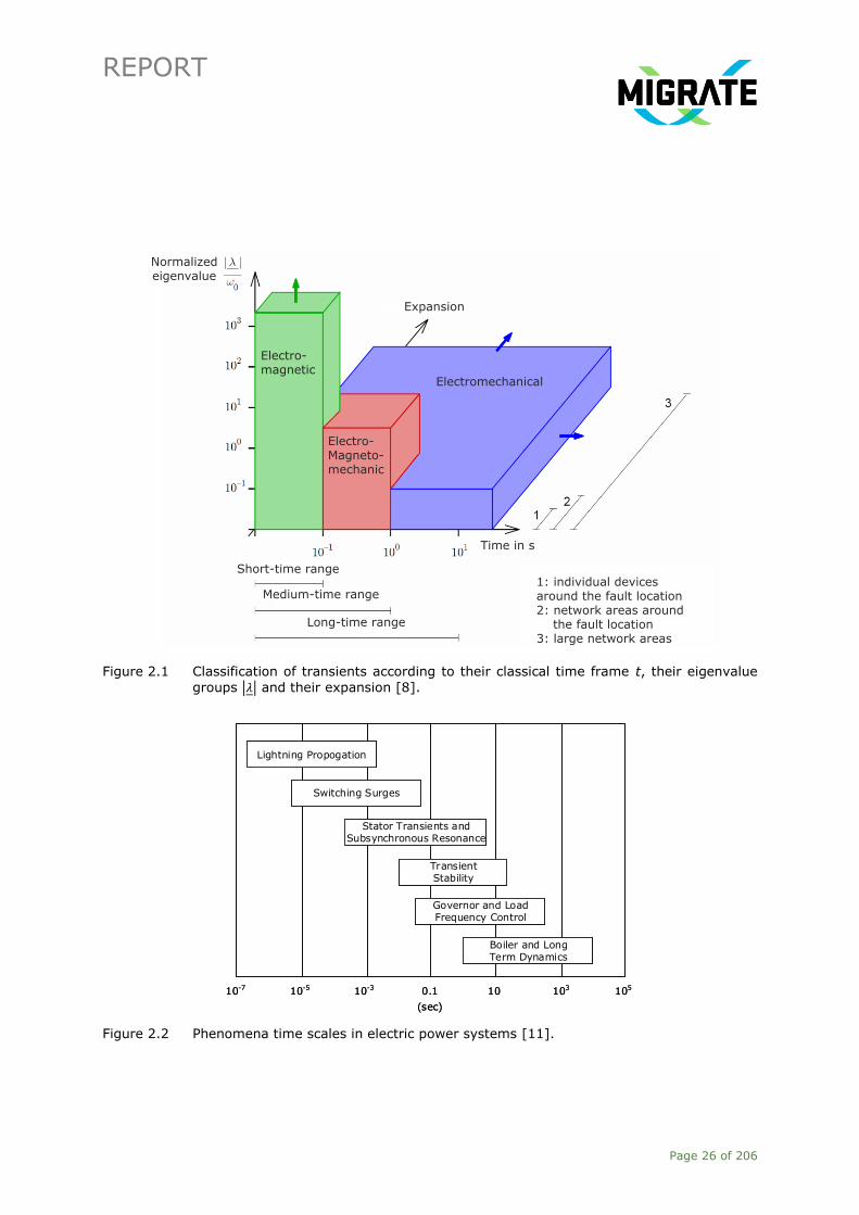
associated with relatively larger grid areas. For instance, in [8], the following three time scales of
the power system are defined:
Short-time range involves fast electromagnetic transients (0.5-500 kHz) caused by energy
exchange between inductive and capacitive energy storages within the electrical network with
the milliseconds range as the time frame of interest.
Medium-time range involves slower interactions between inductive energy storages, rotor
windings and mechanical energy storages. These energy exchanges are referred to as electro-
magneto-mechanical transients (1-100 Hz) with a time frame of interest of seconds.
Long-time range involves exclusively interactions between long-term mechanical energy
storages, such as secondary reserves. These so-called electromechanical transients (0.5-5 Hz)
have the time frame of interest in the minute range.
Figure 2.1 depicts the three time scales described above, their respective eigenfrequencies, their
characteristic transients and their affected network areas. In time-domain simulations, the
representation of the passive electrical network is crucial. To analyse long- and medium-time range
dynamic phenomena, the passive electrical network is sufficiently characterised by its steady-state
behaviour. Therefore, they are generally categorised as quasi-steady-state phenomena (e.g.
transient stability, control procedures, low-frequency oscillation behaviour) and are simulated using
RMS component models. Here, the passive electrical network is represented by steady-state
models and solely the fundamental oscillation of voltages and currents is considered through their
RMS. If the analysis of fast electromagnetic transients (e.g. switching surges, lighting strikes,
ferroresonances7) is the topic of investigation, the power system area of interest is simulated using
electromagnetic transient (EMT) models with a high level of detail. In EMT simulations, in addition
to the dynamics considered in RMS simulations, the dynamic behaviour of passive network
elements is also taken into consideration. Thus, voltages and currents are expressed by their
instantaneous values [9]. Figure 2.2 shows various phenomena and their time scales in electric
power systems.
7 Ferroresonance refers to all oscillation phenomena between non-linear inductances (power transformers, voltage measurement inductive transformers, etc.) and capacitors (cables, long lines, etc.) [10].
REPORT
Page 26 of 206
1: individual devices around the fault location2: network areas around the fault location3: large network areas
Electro-magnetic
Short-time range
Medium-time range
Long-time range
Expansion
Time in s
Normalized eigenvalue
Electromechanical
Electro-Magneto-mechanic
Figure 2.1 Classification of transients according to their classical time frame t, their eigenvalue
groups |𝜆| and their expansion [8].
10-7 10-5 10-3 0.1 10 103 105
(sec)
Switching Surges
Lightning Propogation
Stator Transients and Subsynchronous Resonance
TransientStability
Governor and LoadFrequency Control
Boiler and LongTerm Dynamics
10-7 10-5 10-3 0.1 10 103 105
(sec)
Switching Surges
Lightning Propogation
Stator Transients and Subsynchronous Resonance
TransientStability
Governor and LoadFrequency Control
Boiler and LongTerm Dynamics
Figure 2.2 Phenomena time scales in electric power systems [11].

REPORT
Page 27 of 206
Another essential factor in time-domain simulations is the length of the integration time step which
is linked to the smallest time constants of the system. Due to the higher frequencies that have to
be covered in EMT studies compared to RMS studies, the time steps in EMT simulations need to be
considerably shorter. This is why the passive network elements in EMT simulations are modelled by
their dynamic representation. The dynamic phenomena in medium-time and long-time range can
also be simulated using EMT simulation. The calculation time would increase unnecessarily in this
case. Hence, for an efficient simulation of a certain phenomenon, it is necessary to adjust the
integration time step. For long-term simulations, it is advantageous that computer programmes
support a simulation step size control which increases the step size automatically after fast
transients have decayed [9].
2.3 Power System Simulation Practices
2.3.1 Simulation of Power System Dynamic Response
As mentioned in Section 2.2, in order to analyse long- and medium-time range dynamic
phenomena (quasi-steady-state phenomena), the steady-state representation of passive electrical
networks in the frequency domain is sufficiently accurate (i.e. a set of linear algebraic equations).
In long-time range studies, the performance of transformer tap changers and phase-shifting angle
controls cause variations in the network admittance matrix as a function of bus voltages and time.
In short-time range simulations, the passive electrical network is represented through its EMT
models (i.e. a set of differential and partial differential equations). Static loads are represented also
through algebraic equations and can be represented as part of the network equations (network
admittance matrix) in case of quasi-steady-state studies. The dynamic behaviour of the various
dynamic devices (e.g. generating units, dynamic loads, HVDC converters, static var compensators,
synchronous condensers, their respective controls, etc.) is represented through linear or non-linear
differential equation systems [12]. The network equations, the equations of the dynamic devices
and the equations of the non-linear static loads are interfaced by means of equivalent current
injections of the devices and the non-linear loads with the network. The current injections from the
dynamic devices are dependent on their state variables [13]. The resulting overall system
equations can be solved for each time step as an algebraic-differential equation system can be
solved using a wide range of approaches depending on the modelling details and the numerical
methods [12].
The numerical methods for solving the differential equation system are categorised in implicit (e.g.
trapezoidal rule) and explicit methods (e.g. Euler, Runge-Kutta methods). In [12], a general
description of these methods is provided. A comparison between discretisation using implicit multi-
step methods and numerical integration using explicit methods leads to the following advantages
and disadvantages:
- In contrast to implicit methods which solve the non-linear differential equation systems
iteratively, the numerical integration using explicit numerical methods requires generally lesser

REPORT
Page 28 of 206
computation time per time step. However, to avoid instabilities, the time steps have to remain
small [13].
- Because of the better stability properties of the implicit methods, the step size can be increased
considerably after decaying the fast transients. Therefore, regarding the long-time range
simulations, these methods exhibit major advantages. In these methods, the higher
computation time per time step will be compensated through a lower number of time steps [13].
The standard programs to simulate transients in the power system can be roughly categorised into
programs to analyse electromechanical transients (medium- and long-time range) and programs to
study electromagnetic transients (short-time range). Electromechanical transient programs (e.g.
PSS/E or EUROSTAG) use a steady-state network model. EUROSTAG is capable to analyse the
whole range of electromechanical transients (from a few seconds to minutes), because of its time
step adjustment feature. In principle, electromagnetic transient programs (e.g. EMTDC8) can also
analyse electromechanical phenomena. However, it will not be efficient, because they include a
highly detailed network model whose analysis demands very small time steps. NETOMAC and
DIgSILENT can analyse both electromagnetic and electromechanical transients, because they
support a highly detailed transient as well as a steady-state network model. Other important
factors to be considered with respect to simulation programs are speed and robustness of their
numerical methods as well as completeness of their model library [13].
2.3.2 Review on Current TSO Practices
Since power system stability assessment is a crucial task for every TSO, their current way of
performing dynamic network studies strongly determines the state-of-the-art. The following
summarises the answers of 21 ENTSO-E TSOs given to a questionnaire issued in Q2/2016 9
regarding state-of-the-art modelling and simulation of power system stability.
How are dynamic studies currently performed: RMS or EMT?
Dynamic studies regarding power system stability are predominantly performed in RMS. Classical
stability aspects like frequency stability, voltage stability and rotor angle stability are exclusively
studied using RMS simulation environments. Most (but not all) of the TSOs perform EMT studies as
well, but mostly to study specific phenomena of certain devices like harmonics, saturation effects,
transient overvoltages and switching of extra-high voltage (EHV) cables (often in the planning
stage). However, few TSOs mentioned controller interactions between HVDC converters and WTG
converters or between WTG converters connected to nearby buses to be within the scope of EMT
simulations.
What is the frequency for performing these studies?
The frequency varies widely. Most TSOs perform RMS stability studies a few times a year as part of
the long-term system planning and/or triggered by events. However, one TSO mentions that it
8 EMTDC: Electromagnetic Transients including DC. 9 For more information on the questionnaire and a summary covering the full questionnaire please refer to MIGRATE Deliverable 1.1 “Report on systemic issues” [2].

REPORT
Page 29 of 206
performs RMS dynamic studies in real-time every 15 minutes. The connection of new equipment is
also accompanied by dynamic studies; both RMS and EMT (most often mentioned are HVDC
converters, large wind farms and FACTS).
What stability aspects are being studied?
All classical stability aspects are mentioned in the answers, but most of the TSOs focus on
phenomena they decided to monitor more closely due to special characteristics in their control
zones. In this context, transient stability is most often mentioned, but voltage stability and small-
signal rotor angle stability are often monitored too. Frequency stability is mentioned least often,
but this may be due to the fact that frequency stability is often studied by ENTSO for the whole
regional groups’ synchronous areas. Controller interactions, which have been defined in D1.1 to be
a stability issue, are also mentioned.
What is the geographical size of the grid model you use for the different stability aspects?
Most TSOs of Regional Group Continental Europe (RG CE) use a model of their own control zone
and a (sometimes simplified) representation of their neighbouring control zones for RMS studies.
Some use the ENTSO-E CE dynamic study model covering the whole synchronous area. TSOs of
other RGs typically model the whole synchronous area (except for RG Baltic, where the
neighbouring countries, which are no ENTSO-E members, are not fully represented). Few TSOs
gave an answer differentiated with respect to stability phenomena. However, the answers given
imply a larger size for small-signal rotor angle stability and frequency stability and a smaller size
for transient stability and voltage stability. The geographical size of models for EMT studies
strongly depends on the scope of the study. In general, the geographical size is smaller, often
focusing on few devices and buses.
Which utilities are modelled in which detail? Which control systems are modelled in which detail?
RMS:
Generally, the whole own EHV and sometimes HV network is modelled (overhead lines (OHLs),
cables and transformers). Most TSOs also mention models for SVC and HVDC converters/links
(generic or vendor). Little information is given about the level of detail applied to other control
zones. As some TSOs use a mutual dynamic model, the OHL, cables and transformers are probably
modelled in a similar level of detail. Likewise, little information is given about modelling the
surroundings of the area of detailed modelling. One TSO mentions to use a simplified
representation available from its supervisory control and data acquisition (SCADA) system.
Network protection – if mentioned – is modelled through contingency definitions. Underfrequency
Load Shedding (UFLS) is mentioned to be modelled but without further specification.
Usually, all power plants with synchronous generators are modelled in detail (some TSOs mention
certain thresholds between 5 MW and 100 MW above which the generators are modelled in detail).
Normally, these include models of the synchronous generator, the turbine governor, the turbine,
the excitation system (including PSS) and the AVR. Some TSOs mention to model excitation

REPORT
Page 30 of 206
limiters and protection schemes as well. Several TSOs model large wind farms, usually with generic
models10.
One TSO also models smaller wind clusters and Combined Heat and Power (CHP) clusters with
aggregated models. Typically, the models are more detailed and specific for the TSO’s own control
zone. Generation in neighbouring control zones is often modelled less detailed and parameterised
less specifically.
EMT
Little information is given about the level of detail of EMT models. In general, EMT models are more
detailed and more often provided by the respective device manufacturer or owner.
How is the load currently being modelled for your dynamic studies? Do you have generic models? If so, how is the parameterisation being done? Do you have user defined load models? If so, how is the parameterisation being done?
Usually, the load is modelled as static load, most often with a breakdown into constant power,
constant current and constant admittance components (ZIP load), but some TSOs just use constant
impedance loads. This includes some voltage dependency of the loads. Frequency dependency is
not mentioned by most of the TSOs. User defined load models are normally not used, except in
specific situations for some large industrial loads. One TSO mentions that distributed generation is
modelled separately from the loads (while it is assumed that usually distributed generation is
included in the load model representing the distribution grid it is connected to) for distribution grids
with distributed generation.
2.4 Manufacturer Review of PE Capabilities and Network Codes
Within Deliverable D1.1 [2], several Network Codes where summarised and a list of requirements
for grid-connected Power Electronics (PE) was derived. This list was then preliminarily assessed
from an academic point of view with regard to technical feasibility and impact on PE manufacturers.
The results emphasised that requirements, which could demand additional energy storage, could
cause greater efforts by the manufacturers and that several requirements are broadly defined,
leading to uncertainties regarding the consequences for the minimum required capabilities.
Within the framework of Deliverable 1.2, ABB, Enercon, Siemens Energy Management, SMA and
Woodward were consulted as representative manufacturers of a variety of typical grid-connected
PE devices. During the discussion, the manufacturers commented on the preliminary assessment
done in D1.1 and provided an assessment of the new requirements from their point of view as well
as comments on additional PE capabilities, which are not required yet, but are available. For each
additional feature, an assessment whether it can be activated with little cost or whether it requires
10 One TSO explicitly mentions to use WECC 2nd generation model: Electric Power Research Institute (EPRI), “Specification of the Second Generation Generic Models for Wind Turbine Generators,” 2014. [available Online].

REPORT
Page 31 of 206
an elaborate development process has to be made. In addition, general aspects of grid operation
with a high share of PE devices were discussed.
In this section, the anonymised results of these discussions are summarised, in order to reflect the
manufacturer’s comments regarding PE capabilities within the framework of the Network Codes. It
therefore reflects the opinion of the manufacturers, not necessarily the authors’ opinion. During the
talks, the requirements have been discussed individually. However, it proved feasible to group
several requirements and categorise them. The discussed requirements and their assigned
category within this section are depicted in Table 2.1.
Many requirements match existing technology or require minor adjustments. These are categorised
as already implemented. Requirements, which are not considered to pose difficulties, but which
have not been implemented yet, are marked as firmware modifications. Changes to the systems,
requiring major hardware or software extensions are described as system extensions. System
resizing describes requirements, like new voltage ranges, which may lead to a redesign of system
components. Several requirements may ask for additional power and therefore a power reserve or
energy storage can become necessary, depending on the concrete specification by the relevant
TSO. Some manufacturers stressed that technical capabilities will only be available in the field if
the operators of the plants either have to provide them compulsory (due to Network Code
requirements), or it is financially attractive to them.
Table 2.1 Overview of the discussed requirements and their assigned category; Brackets () indicate technology dependence or partial applicability.
Group
Requirement
Exh
au
sti
ve
req
uir
em
en
t
Alr
ead
y
imp
lem
en
ted
/
min
or c
on
cern
Fir
mw
are
mo
dif
icati
on
Syste
m
resiz
ing
Syste
m
exte
nsio
n
Po
wer r
eserve/
en
erg
y s
tora
ge
Frequency ranges X X (X)
Rate of change of frequency withstand
capability X
Limited frequency sensitive mode –
overfrequency X X
Constant output at target active power X X
Maximum active power reduction at
underfrequency X
Active power controllability and control range X X
Limited frequency sensitive mode –
underfrequency X X
Frequency sensitive mode X X
Frequency restoration control X

REPORT
Page 32 of 206
Group
Requirement
Exh
au
sti
ve
req
uir
em
en
t
Alr
ead
y
imp
lem
en
ted
/
min
or c
on
cern
Fir
mw
are
mo
dif
icati
on
Syste
m
resiz
ing
Syste
m
exte
nsio
n
Po
wer r
eserve/
en
erg
y s
tora
ge
Disconnection of load due to underfrequency X X
Fault-ride-through capability of power-
generating modules connected below 110 kV X
Fault-ride-through capability of power-
generating modules connected at 110 kV or
above
X
Loss of stability11 X
Rate of change of active power X (X)
Steady-state stability1 X X
Auto-reclosures X (X)
Black start capability11 (X) X X
Capability to take part in isolated network
operation11 (X) X
Quick re-synchronisation11 X
Voltage ranges X X
Synthetic inertia capability11 (X) X X
Post-fault active power recovery X
Provision of fast fault current11 X
Priority to active or reactive power
contribution (X) (X)
Reactive power capability at maximum active
power X
Reactive power capability below maximum
active power X
Reactive power control modes X
Power oscillation damping control (X) X
System Resizing
Several requirements can be addressed by the inverter’s sizing, i.e. expanded 𝑈-𝑄/𝑃max-profiles
require higher rated modules for the same active power rating of the inverter. In addition, the new
frequency ranges are generally considered to be a minor concern for PE devices, but may require
modification of auxiliary systems like pumps. With the expected deviations from nominal grid
frequency, the tuning of filter components may have to be revalidated. The larger frequency
11 The requirement was considered to be not sufficiently specified, allowing different interpretations.

REPORT
Page 33 of 206
deviations at higher harmonics may impair the output filter’s effectiveness or even excite parallel
resonances within the filter, causing large currents. The new voltage ranges do not match the
existing portfolio of available voltage classes of devices, causing an oversizing of components or
extra redesign effort. This is especially important for high-voltage facilities, as the required
minimum times at a voltage of 1.15 pu could lead to significantly oversized insulations.
Firmware Modifications
Features like Limited Frequency Sensitive Mode – Overfrequency (LFSM-O) or the priority of
reactive/active power contribution are considered to be technically feasible, but have to be
implemented. LFSM-O could be challenging for systems with a power source which cannot be
powered down dynamically, which is especially important when considering technologies apart from
Wind, PV or HVDC systems.
Even though some requirements can be fulfilled with firmware modifications, every new or updated
feature increases cost. Each modification needs to be thoroughly tested and certified, if required,
which was mentioned to be the most time-consuming part of implementation.
System Extension
Synthetic inertia capability, black start capability and the capability to take part in islanded
operation can cause significant effort in order to be implemented. It is important to note that these
requirements are non-exhaustive12 and they only apply, if demanded by the relevant TSO13. The
unspecific character of these requirements led to different interpretations of what is demanded
from PE devices.
It is important to distinguish between participating in islanded network operation and guiding
islanded network operation. Taking part in islanded operation was not considered to be generally
implemented in installed devices, but technically feasible. Guiding an isolated network is impacted
by the power capability of the grid forming entity14. Larger power sources have greater influence
on the isolated network operation, but are not necessarily designed for this operation. Therefore,
guiding isolated network operation is considered as more complex and technically challenging, as
there can be other power generating entities of larger power capacity within the isolated network
which do not operate as part of the grid forming collective and need to be synchronised. An
additional remark was made regarding devices connected at distribution level. The requirements
set by the Distribution System Operator (DSO) often demand the immediate disconnection in case
of islanded operation due to health and safety reasons. The priorities of the requirements should be
specified.
Black start capability strongly depends on the system’s power source. Additionally, modifications to
the auxiliary systems or energy storages could become necessary. The concepts are not generally
12 They are subject to further - more detailed - specification by the relevant TSO 13 Regulation (EU) 2016/631 14 Single or group of power generating units, collectively forming the grid

REPORT
Page 34 of 206
implemented in existing hardware, but are imaginable for suitable technologies in the future, e.g.
Photovoltaics (PV). Technologies for isolated network operation or black start capabilities are
already available from microgrid concepts, uninterruptable power supplies or are already
implemented in High-Voltage Direct Current (HVDC) stations. Wind turbines and PV, as installed
today, lack energy storages and/or grid forming capability can therefore not black start directly or
at all times. As soon as the local grid is energised by another power source, they could contribute
to the black start.
Synthetic inertia can be requested to mimic the frequency-response reserve of conventional
generators. Some TSOs tend towards an implementation based on the rate of change of frequency,
but currently an implementation based on the deviation of frequency is accepted in many cases. If
an implementation based on the deviation of frequency is accepted, this requirement could also be
fulfilled by operating in a fast Frequency Sensitive Mode (FSM). An implementation based on the
rate of change of frequency may pose some difficulties regarding the filtering effect of the applied
calculation method, especially when considering existing Phase-Locked Loop (PLL) technology. A
detection time of 50 to 70 ms was mentioned for changes in frequency, but which strongly depends
on the implementation. It is assumed to be demanding to design an effective and robust synthetic
inertia based on this without getting susceptible to inadvertent reaction in case of fault events that
affect the frequency measurement. If the inverter operates as a voltage source, the initial reaction
could be very fast, but its current needs to be controlled strictly to never exceed the maximum
currents admitted by the PE. If concepts for synthetic inertia are used, which draw additional power
from the rotational energy of the system - thereby slowing it down [14] - additional specifications
for tolerances and recovery periods are needed.
Power oscillation damping control is already implemented in HVDC converters, but not in other PE
devices.
Power Source / Energy Storage
Many requirements can be interpreted in such a way that they make an energy storage system or
power reserve necessary. FSM and Limited Frequency Sensitive Mode – Underfrequency (LFSM-U)
require the capability to increase the output power. The LFSM-U requirement accounts for the
operating conditions of the device and the availability of prime energy. ENTSO-E described the
possibility that only power-generating units operating below maximum available power activate
LFSM-U [15].
Power reserves can be implemented by energy storages or by reducing the output power below the
maximum available power in normal operation. HVDC links have a power reserve implemented,
decreasing the transmission line’s capacity. Other concepts, i.e. using the rotational energy of a
wind turbine, allow an increased output power for a limited time, without additional energy
storages or withholding power. Actively operating below the maximum available power requires a
determination of the maximum power point at the present operating conditions. Depending on the
power source, this estimation is already possible or technically challenging.

REPORT
Page 35 of 206
Limiting the rate of change of active power in upward direction is usually already implemented. The
limitation in downward direction is generally not expected to be demanded from volatile energy
sources and would likely make an energy storage system necessary. Limiting the rate of change of
active power in upward direction can decrease the yield, if power peaks cannot be fed into the grid.
If additional storages are necessary or power is withheld actively, the investment cost of the PE
devices rise and/or the yield decreases.
Additional Comments from the Manufacturers
In addition to the already described requirements, comments were made to features that are
already implemented in PE devices and other topics regarding technical capabilities of grid-
connected PE devices.
Fault-ride-through capability is implemented by all manufacturers. This also applies to type 3
wind turbines. The variety of existing Fault-Ride-Through (FRT) profiles increases the effort of
implementation and testing.
The rate of change of frequency withstand capability of PE devices is generally mentioned to be
higher than the requirement for HVDC converter stations, but it has to be noted that a high rate
of change of frequency is likely to occur in correlation with power imbalances within the grid. If
the PE-connected power generating module operates in FSM during the high rate of change of
frequency, a sufficiently dynamic power source is required. Additionally, the demanded
dynamics for FSM are not specified sufficiently.
The specifications to determine frequency were considered to be insufficiently precise by some
manufacturers. Depending on the implementation and filter settings, varying results of the rate
of change of frequencies can be generated. This is especially important, if the phase angle at
the connection point jumps.
PE devices allow a wide and dynamic control of active and reactive power. In general, the
necessary control interfaces are already implemented in the firmware of existing devices. In
order to control a great number of PE devices within the grid, appropriate communication
infrastructure has to be provided.
The disconnection of load is uncomplicated for PE devices, and it was mentioned that HVDC
links can even initiate a fast power reversal, if necessary.
The requirement to automatically disconnect in case of angular instability or loss of control was
interpreted in different ways. One interpretation was correlated to angular stability, which is
already implemented in the devices implicitly. In case of large deviations between the detected
and actual phase angle, overcurrents will occur and the device disconnects. Active detection
methods for persisting output oscillations are not implemented. Another interpretation was with
regard to active and reactive power controllability. Depending on the grid quality and present
configuration, e.g. the amount of power injected by devices in close electrical proximity, not all
operating points in the PQ diagram can be operated stably, with regard to other system
limitations, i.e. voltage ranges. It is assessed to be difficult to determine the present distance to
unstable operating conditions within the PQ diagram

REPORT
Page 36 of 206
Auto-reclosures can be handled by all manufactures, if these are limited to a period of a few
seconds. For larger facilities, i.e. HVDC systems, this requirement is unproblematic, as the
facility is connected via multiple paralleled lines. For system sizing and design, more precise
specifications including type, distance and number of faults would be advantageous.
The interpretation of quick resynchronisation showed differences from manufacturer to
manufacturer. A common understanding was that resynchronisation can be done significantly
faster than conventional generation, if the protection devices are set up appropriately.
Several manufacturers mentioned rise times of fast fault currents around 30 ms. A discussed
rise time of 10 ms was considered to be difficult to implement with state-of-the-art control
concepts. Converters operating as voltage sources could react very quickly in fault conditions.
The provided fault current was often assessed to be 1.2 to 1.3 times the nominal current. There
are also devices that provide a fault current equal to the nominal current. Some devices are
designed to provide this overcurrent permanently, whereas other devices cannot. An important
note was that PE devices are often not operating at maximum capacity, which is why the
effective short circuit ratio is likely to be much higher than 1.2 to 1.3 times the presently infeed
current in most situations.
One manufacturer mentioned that today’s network codes and requirements are designed with
grid-feeding controls in mind and impede the implementation of novel control techniques,
especially with regard to harmonic content. Some requirements and characteristic parameters
were designed considering stiff grids and may need reassessment for applicability in weak grids.
It was also mentioned that the new codes are rather a step towards decentralised generation
than to renewable energy sources. Further, the question was raised, whether it may be more
cost-efficient to aggregate some of the features in larger, specialised facilities, i.e. energy
storage systems or reactive power provision.
Table 2.2 shows a selected number of features and whether they are available in different
technologies. As the discussed HVDC technology is a transmission system only, the remarks for
voltage source converter HVDC systems assume that the HVDC link is energised and power is
available at the other point of connection.
The technical feasibility of many non-exhaustive requirements depends on the concrete
specifications demanded by the relevant TSO, which is of significant importance for requirements
that may demand an energy storage, i.e. frequency sensitive modes. As long as active power
increments are expected only when additional power is available, these requirements are
considered to be technical feasible. If active power increments are demanded at any time, either
additional energy storages are needed to increase power for a limited period or an active power
reserve has to be created by withholding available power. This increases the investment cost or
decreases yield.

REPORT
Page 37 of 206
Table 2.2 Availability of several grid features with regard to different technologies.
Type of generation
Requirement
Win
d
PV
HV
DC
15(V
SC
)
Active power controllability and control range
Limited frequency sensitive mode – underfrequency ●/16 ●/16
Frequency sensitive mode ●/16 ●/16
Frequency restoration control ●/16 ●/16
Priority to active or reactive power contribution ●
Quick re-synchronisation
Black start capability 16 ●16
Capability to take part in isolated network operation17 ● ●
Synthetic inertia capability ●16 ●16
Power oscillation damping control ● ●
: Already possible with existing technology, but may require minor modifications
● : Not implemented at the moment, but considered technically feasible
: Only implementable with great effort/cost
Voltage source converter based HVDC systems are capable of providing manifold advantageous
features for grid stability. It has to be kept in mind that HVDC converter stations usually are large
facilities with high power rating and computing power. Some advanced control features may not be
transferable to a great number of small power generating units without additional investment in
processing hardware, communication and implementation effort. Nevertheless, e.g. VSC based
battery systems could provide similar advantageous features.
Different concepts of PE generation to take part in islanded operation are currently investigated
broadly, i.e. microgrids. The overall consent of all manufacturers was that the benefit of each
requirement for the particular grid application has to be weighed against the cost of
implementation and testing.
2.5 Conclusions
In this chapter, the state-of-the-art modelling of power systems and the capabilities of Power
Electronics (PE) were described. The analysis of the state-of-the-art in power system modelling and
simulation showed that stability analyses of large power systems typically are performed using
RMS models. The concrete modelling depth and geographical extent of the grid model differ
15 With regard to HVDC interconnections between asynchronous grids; available features of embedded
HVDC links may vary. 16 The technical feasibility and necessary effort depends on whether an additional energy storage or
power reserve is requested by the relevant TSO, as it would greatly increase investment cost and/or yield. As long as fluctuations of available primary energy are accepted, the requirements are technically feasible.
17 With respect to the distinction between “taking part” and “guiding” isolated network operation.

REPORT
Page 38 of 206
depending on the analysed stability phenomenon and grid area under study and data availability.
However, stability phenomena significantly influenced or even caused by PE devices might not be
sufficiently analysable with RMS models, e.g. PE controller interactions. The state-of-the-art must
therefore be scrutinised with respect to the effects of increasing PE penetration. The validity of key
assumptions justifying RMS simulations must be reviewed as well as the validity of the applied
component models.
In a manufacturer review, the capabilities of PE with respect to the network code were discussed.
The technical feasibility of many non-exhaustive requirements depends on the concrete
specifications demanded by the relevant TSO, which is of significant importance for requirements
that may demand an energy storage. Voltage source converter based HVDC systems are capable of
providing manifold advantageous features for grid stability, but it has to be kept in mind that some
advanced control features may not be transferable to a great number of small power generating
units without additional investment in processing hardware, communication and implementation.
Different concepts of PE generation are currently and broadly researched and the benefit of each
requirement for the particular grid application has to be weighed against the cost of
implementation and testing.

REPORT
Page 39 of 206
3 Modelling of Transmission Systems with high
Penetration of PE Devices
3.1 Introduction
The MIGRATE project has four main objectives of which the first one is related to the development
of a methodology to be shared with TSOs that allows an improved understanding and monitoring of
the system dynamic behaviour [1]. This specific objective requires a systematic study approach
that can be reproduced by all partners of the consortium, and for such purpose the definition of
"model problems” is relevant. The model problems describe the modelling, case study and
simulation/quantification used to analyse a specific stability phenomenon. In Section 3.2, the
modelling approach and characteristics of the set of generic test cases developed based upon
existing benchmark systems for stability studies is provided. The case study and simulation results
are presented in Chapter 4, which use the generic test cases for investigation of the impact of PE
on the phenomena listed in Table 1.2 (Chapter 1) and to define the features of the methodology to
be used for the determination of the KPIs. To study the impact of increasing levels of Power
Electronics on the Great Britain system, transition scenarios from 2016 until 2030 are developed
based on a reduced size model of the GB system, whereas the situation in the year 2016 is
considered in a relatively detailed model of the Irish system. These implementations are presented
in Section 3.3. In Chapter 4, the outcomes of the tests of the proposed KPIs on the GB and Irish
systems are provided.
3.2 Development of Generic Test Cases
3.2.1 General Description of Generic Test Cases
The model problems, as defined in deliverable D1.1 of MIGRATE, are the descriptions of the
modelling and simulation needs to ensure accurate recreation of a given stability phenomenon
when the studied system is close to, or in, an unstable condition [2]. A model problem has three
main aspects: the modelling, case study and simulation/quantification. Figure 3.1 shows an
overview of the model problem definition. It can be seen that the modelling aspect describes how
the system and its components are modelled. The case study specifies the grid topology and
conditions under which instability occurs, while the simulation/quantification aspect describes how
the simulation is performed and how the results are assessed. The detailed information provided is
intended to fulfil Objective 1 as stated in the MIGRATE Grant Agreement, where the modelling
technique of all elements is required to be known in order to understand the dynamics of the
considered system and to allow the reproducibility of the tests [1].
This chapter introduces generic test cases and validation systems to study the stability behaviour
of power systems for the selected phenomena shown in Table 1.2 (Chapter 1). As modelling of
these systems and their elements are essential for this, in this chapter special attention is paid to
the Modelling aspect of the model problem. Concerning the case study aspect, the grid topology
and (initial) operating conditions under which instability can occur are the parts that will be

REPORT
Page 40 of 206
discussed in this chapter as well. As the conditions under which instability occurs can only be
determined by analysing the systems with the stability KPIs, part of the case study aspect will be
described in Chapter 4. The simulation/quantification aspect of the model problem is specific for
the particular study and used indicators, and will therefore be discussed in Chapter 4 as well.
Figure 3.1 Overview of the model problem.
In the following sections, generic test cases will be developed. These generic test cases consider
the specific stability phenomena, typically classified as the study of frequency, rotor angle and
voltage stability [3]. Sub-synchronous controller interactions are a fourth category considered in
this research. Each particular phenomenon must be studied separately for better understanding of
the roots and propagation of stability threats.
3.2.2 Power System Modelling in RMS and EMT
The modelling aspect refers to the representation of the electrical system, the considered devices
and their associated controllers that will be implemented for the stability studies. Frequency, rotor
angle and voltage stability are studied with RMS simulations in DIgSILENT PowerFactory, while
sub-synchronous controller interactions are studied with EMT simulations in PSCAD. The following
sections describe the general modelling in PowerFactory and PSCAD, where special attention is paid
to the modelling of wind turbines.

REPORT
Page 41 of 206
Modelling in PowerFactory
Frequency, rotor angle and voltage stability are studied by implementing models for RMS
simulations in PowerFactory. Table 3.1 gives an overview of the selected elements in DIgSILENT
PowerFactory 2016 for implementing the generic test cases as well as the GB system and the Irish
system. Particular modelling aspects are highlighted in the subsection describing each system in
the remainder of this chapter.
Table 3.1 Power system modelling in PowerFactory.
Element Details Reference
Synchronous generator ElmSym / TypSym (6th-order)
(controllers: AVR, GOV, PSS)
[16]
Automatic Voltage Regulator (AVR) Modified IEEE Type 1 (avr_IEET1A.BlkDef
model taken from the library of standard
models)
[17]
Turbine governors (GOV) Steam (gov_TGOV1.BlkDef model taken
from the library of standard models) /
Hydro (gov_HYGOV.BlkDef model taken
from the library of standard models)
[17]
Power System Stabiliser (PSS) Speed input stabiliser (user defined model
based on pss_PSS1A.BlkDef model taken
from the library of standard models)
[12], [17]
Static Var System (SVS) ElmSvs [18]
Two-winding transformer ElmTr2 / TypTr2 (3-phase) [19]
General loads ElmLod, TypLod [20]
Transmission lines ElmLne / TypLne
(PI-circuit, lumped parameters)
[21]
Nodes connecting lines, generators,
loads, etc. to the network
ElmTerm [22]
Phase-Locked Loop (PLL) ELMPhi_pll (first-order or second-order
generic models might be used)
[23], [24]
More details and typical parameters for the generic test cases can be found in Appendix A.
To describe the overall approach for interconnecting the necessary elements to perform RMS
simulation, a simple example is given in this section. Consider a system with two synchronous
machines and one Wind Park model (WP) in a network with auxiliary PLL block for measuring the
frequency. The synchronous machines in the network have auxiliary components such as AVRs,
PSS and governor systems and the same holds for the WP, which has a measurement unit,
mechanical part and P/Q controllers. The hierarchical structure of DIgSILENT Simulation Language
(DSL) is used to generate a model of the auxiliary components attached to each device and to

REPORT
Page 42 of 206
ensure correct execution of time domain simulations. The hierarchical levels defined by DSL are
associated to Model Definition, Common Model, Composite Frame, and Composite Model.
In this example, as well as in all implemented models (generic test cases, GB system, Irish
System), all synchronous machines in the network have a similar structure, defined as Composite
Frame in PowerFactory, which defines slots for how the AVR, the PSS and the governor system are
connected to the machine. A Composite Frame as shown in Figure 3.2 for all the synchronous
machines and the WP model can be defined. This composite frame is located in the User Defined
Models folder inside the project Library. The Composite Frame can be conceived as some kind of
draft (which can be easily modified), that is called from an object called Composite Model, which
constitutes some kind of mask that actually allows to PowerFactory to select the model of the
device or machine and its associated auxiliary components (i.e. controller, protection devices, and
objects for external data exchange) to be considered in the simulation functions. These composite
models are located inside the Network Data folder.
NETWORK
Static Generator
(WP)
Mechanical Model
Synchronous Generator1
Exc. 1
LFC
PSS
AVR
Synchronous Generator1
Exc. 1
LFC
PSS
AVR
Common Models Common Models
Composite Model 3Composite Model 2Composite Model 1
ControlP, Q, Pitch Measurments
Library
Synchronous Generator1
Exc. 1
LFC
PSS
AVR
Composite Frame
Static Generator
(WP)
ControlP, Q, Pitch Measurments
Composite FrameAVR PSS GOV
P,Q controller
WP Control
Inertia Emulation
Model definitions
Input data
Input data
Mechanical Model
PLL
Figure 3.2 General example of the DSL components implementation.
Model Definitions are block diagrams that define the skeleton of auxiliary models. AVR, PSS and
governor models are defined as model definitions and stored in the User Defined Models folder
inside the project Library similar to composite frames. Each Model Definition includes the transfer
functions and control systems equations to be implemented. PowerFactory provides macros with
most of standard transfer functions. The macros allow defining input signals, output signals,
parameters, internal variables, state equations, state variables, and minimum/maximum limits. In
this example, for each of the two synchronous machine’s Composite Models, the AVR (and PSS,
governors) may have different values of parameters. Common models are objects that fill up the
slots in the Composite Model for each machine, creating an integrated model in the time domain.

REPORT
Page 43 of 206
The structure of Common Models is borrowed from Model Definitions. Thus, each of the AVR, PSS,
and governor Common Models picks up its respective model blueprint (or structure) from the Model
Definition. To summarise: Composite Models borrow their structure from Composite Frames and
Common Models borrow their structure from Model Definitions. Common Models are filled in slots
available in Composite Models. The above example is visualised in Figure 3.2.
Wind Turbine Model in PowerFactory
The wind turbine models used in MIGRATE WP1 were developed in DIgSILENT PowerFactory by
Energynautics GmbH based on the standard IEC 61400-27 series [25]. The developed model is
embedded into a single structure following the principles of DSL, and is used to represent different
types of turbines, being possible to change the type of the wind turbine (Type 3A, 3B or 4) by
changing the generator system. This section gives a brief explanation of the models included in the
generic test cases which are used in RMS simulations, also showing some simulation results that
illustrate the model performance (i.e. initialisation and dynamic response to a disturbance).
Single Wind Turbine Model in PowerFactory
The structure of wind turbine model is presented in Figure 3.3 [26]. The main features of the
model are described as follows:
─ In the measurement part of this model, the blocks Frequency, PowerMeasurement and
VoltageMeasurement are connected directly to the terminals of the wind turbine and put out the
corresponding measurement data. Those measurement values and the currents from the
Generator Block are used for initialising the model.
─ The Generator Block contains the PowerFactory element “Static Generator”, and works as a
current source. The Generator System block is taken from IEC 61400-27-1 [26], [27].
─ The mechanical part is represented by the Aerodynamic block, which calculates the mechanical
power on the turbine, and the Mechanical block, which contains a two mass or single mass
oscillator. The Two mass model is based on IEC 61400-27-1 [27].
─ Input part: the block Wind speed gives the wind speed. It must contain an external file with
wind measurement data in m/s. As an alternative to wind speed as input, the maximal available
power can be used as input by using Power input. In Input choice and back calculation one of
the two input options can be chosen.
─ In the control part, the block P control is based on P control Type 3 from [25]. In this study, it is
used for both Type 3 and 4 wind turbines. The Pitch angle control block is taken mainly from
[25]. The input pemuin is added to pWTref (the active power reference value) when emulated
inertia is activated. There are several possibilities for power control depending on the frequency
inserted. These possibilities are P choice and reduction (power reduction with overfrequency)
[28], Delta control [29], and Emulated Inertia based on [30]. These all influence the output
power depending on the measured frequency.
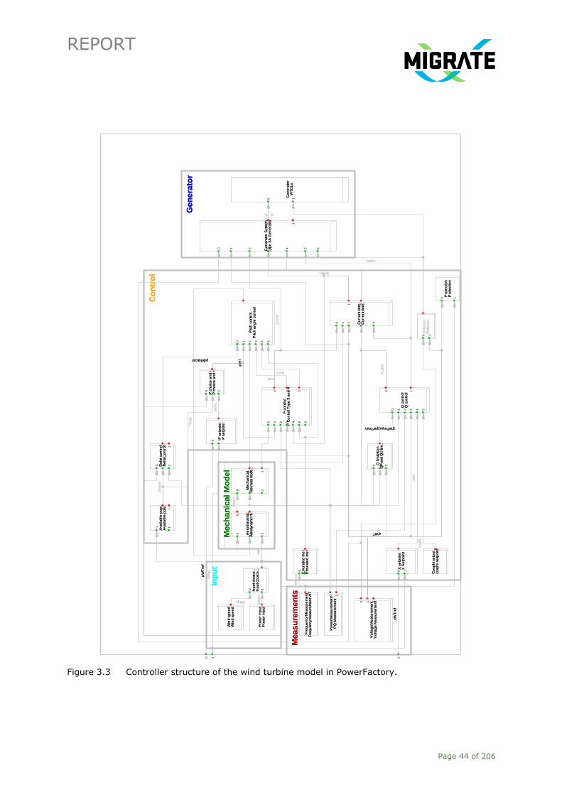
REPORT
Page 44 of 206
Figure 3.3 Controller structure of the wind turbine model in PowerFactory.
Type 3
and 4
Contr
olle
r: 5
.5.4
.2 (
2015)
Po
we
rMe
asu
rem
en
tP
Q M
ea
sure
me
nt
Type 3
and 4
Contr
olle
r: 5
.5.4
.2 (
2015)
Vo
lta
ge
Me
asu
rem
en
tV
olta
ge
Me
asu
rem
en
t
Me
cha
nic
al
Tw
o m
ass
mod
e..
Ge
ne
rato
r S
yste
mT
ype
3A
Ge
ne
rato
r
Pitch
co
ntr
ol
Pitch
an
gle
co
ntr
ol
Q lim
itatio
nQ
P a
nd Q
U lim
..
P c
on
tro
lP
Co
ntr
ol T
ype
3 a
nd
4
Em
ula
ted
In
er.
.E
mu
late
d In
er.
.
Cu
rre
nt lim
it..
Cu
rre
nt lim
it..
Fre
qu
en
cyM
ea
sure
me
nt
Fre
qu
en
cym
easu
rem
en
t W
T
Co
sph
i se
tpo
i..
cosp
hi se
tpo
int
Ae
rod
yna
mic
Aer
odyn
amic
m..
X s
etp
oin
tX
Se
tpo
int
Win
d s
pe
ed
Win
d s
pe
ed
Ava
ilab
le p
ow
..A
vaila
ble
po
w..
De
lta
co
ntr
ol
De
lta
Co
ntr
ol
Q c
on
tro
lQ
co
ntr
ol
Pro
tect
ion
Pro
tect
ion
P s
etp
oin
tP
se
tpo
int
P c
ho
ice
an
d r
..P
ch
oic
e a
nd
r..
Ge
ne
rato
rW
T0
1a
Po
we
r in
pu
tP
ow
er
inp
ut
Inp
ut ch
oic
e ..
Inp
ut ch
oic
e ..
Refe
renc.
.R
efe
renc.
.
cosph..
wref
pord
qWT
FLVR
T
qWTmax;qWTmin
iqmax..
id_re..
ipcm
d
cosp
h..
Th
eta
xre
f
fme
as
pa
vail
pdeltacon
pin
pu..
pa
ero
vWinp..
vW
pre
f
pre
fe..
xWT
ref
pW
Tre
f
WPac
t..
Co
ntr
ol
Mech
an
ical
Mo
de
l
Ge
ne
rato
r
Meas
ure
men
ts
Inp
ut
Inp
ut
Meas
ure
men
ts
Ge
ne
rato
r
Mech
an
ical
Mo
de
l
Co
ntr
ol
Refe
renc.
.R
efe
renc.
.
0 1
Inp
ut ch
oic
e ..
Inp
ut ch
oic
e ..
0 1P
ow
er
inp
ut
Po
we
r in
pu
t
Ge
ne
rato
rW
T0
1a
0 1
P c
ho
ice
an
d r
..P
ch
oic
e a
nd
r..
0 1 2P
se
tpo
int
P s
etp
oin
t
0 1
Pro
tect
ion
Pro
tect
ion
0 1
Q c
on
tro
lQ
co
ntr
ol
0 1 2 3
0 1
4 5
De
lta
co
ntr
ol
De
lta
Co
ntr
ol
0 1 2
0 1
Ava
ilab
le p
ow
..A
vaila
ble
po
w..
0
0 11
Win
d s
pe
ed
Win
d s
pe
ed
X s
etp
oin
tX
Se
tpo
int
0 1
Ae
rod
yna
mic
Aer
odyn
amic
m..
0 1 2
0 1
Co
sph
i se
tpo
i..
cosp
hi se
tpo
int
Fre
qu
en
cyM
ea
sure
me
nt
Fre
qu
en
cym
easu
rem
en
t W
T
Cu
rre
nt lim
it..
Cu
rre
nt lim
it..
0 1 2 301
4
Em
ula
ted
In
er.
.E
mu
late
d In
er.
.
0 1
P c
on
tro
lP
Co
ntr
ol T
ype
3 a
nd
4
0 1 2 3 4
0 1 25 6
Q lim
itatio
nQ
P a
nd Q
U lim
..
0 1 2
Pitch
co
ntr
ol
Pitch
an
gle
co
ntr
ol
0 1 2 3 4 5G
en
era
tor
Sys
tem
Typ
e 3
A G
en
era
tor
0 1 2 3 4 5 6
0 1
Me
cha
nic
al
Tw
o m
ass
mod
e..
0 10 1
2
Vo
lta
ge
Me
asu
rem
en
tV
olta
ge
Me
asu
rem
en
t0 1 2
Po
we
rMe
asu
rem
en
tP
Q M
ea
sure
me
nt
0 1
Type 3
and 4
Contr
olle
r: 5
.5.4
.2 (
2015)
20 1W
Pac
t..
pW
Tre
f
xWT
ref
pre
fe..
pre
f
vW
vWinp..
pa
ero
pin
pu..
pdeltacon
pa
vail
fme
as
xre
f
Th
eta
cosp
h..
ipcm
d
id_re..
iqmax..
qWTmax;qWTmin
FLVR
T
qWT
pord
wref
cosph..
DIgSILENT

REPORT
Page 45 of 206
Some of the input slots require external data (P setpoint, X setpoint, cosphi setpoint, Wind speed
and Power input). For all of these slots, an instance of the PowerFactory type “Measurement File”
(ElmFile) has been created. Those measurement files refer to an external csv-file that contains a
time dependent value. For example, the measurement file for wind speed is inserted in the Wind
speed slot. The first column of the csv-file contains a value for the time (in seconds) and the
second column contains a value for the wind speed (in m/s). All other csv-files that are used by
other measurement files have the same structure. The user can update the csv-files as desired to
create a different wind speed profile. Figure 3.4 shows an example on how to call an external file.
Figure 3.4 External data file selection of wind turbines in PowerFactory.
The template of the model consists of the complete wind turbine including a mechanical part,
generator, controllers and a transformer. The interface which connects the power plant to the grid
model is shown in Figure 3.5. As wind generator, the built in PowerFactory module Static Generator
(ElmGenstat) is used. A two winding transformer (ElmTr2, [19]) is also used.
Figure 3.5 Interface for the connection of the wind model to the grid.

REPORT
Page 46 of 206
Wind Park (WP) model
As it is well known, the use of a single wind turbine is not considered in transmission systems
because of its practicality and low power generation. Instead, the use of a group of wind turbines
at the same location to produce larger amounts of electric power is widely implemented and a
trend in developed countries. This last concept is called a Wind Park (WP) or wind farm.
The WP model aggregates many wind turbines of the same type into one model with one
overarching controller frame, which represents an increased efficiency in the use of computational
resources. Also, an important difference between the software based model between the WP and
wind turbine is that the former controls the active and reactive power at the Point of Common
Coupling (PCC) and not at the terminals of the wind turbine. The general structure of the wind park
control used in PowerFactory is shown in Figure 3.6.
Figure 3.6 Structure of WP controller proposed by IEC 61400-27-1.
As shown in Figure 3.6, the blocks Power measurement, Frequency measurement and Voltage
measurement are connected to the PCC. Hence, the external files that are inserted in P setpoint WP,
X setpoint WP and Cosphi setpoint WP give reference values for the PCC [25].
The interface to the grid, when simulating a whole wind park is depicted in Figure 3.7. Only the
part marked by the red rectangle is part of the template. Therefore, for grid integration, the wind
turbines have to be added separately by inserting the wind turbine templates.
WP control and communication frame:
Communication..Comm delay fo..
Frequency..Phase Mea..
P setpoint WPP setpoint WP
X setpoint WPX Setpoint WP
Cosphi setpoint WPCosphi setpoint WP
WP Q controlWP Q control
Activ eActiv e
Communication..Comm linear f . . xPDre..
y1=
0...
y1=0...
cosp
h..
yo=1...
pWPre..
xWPre..
Communication..Comm linear f . .
Grid measurem..Grid measurem..
pWP
fi..
qWP
fi..
uWP
fi..
FWPU
V..
xPDre..
pPD
re..
fWP
fi..
pWPfi..
qWPfi..
uWPfi..
fWPfi..
p=1.0..
q=-0...
u=1.0..
pPDre..
fmeas..
WP control and communication frame:
Power mea..PQ Measur..
Voltage m..Voltage M..
WP P controlWP P control
Grid measurem..Grid measurem..
0
1
2
3
0
1
2
3
Communication..Comm linear f . .
0
1
2
3
0
1
2
3
Communication..Comm linear f . .
0
1
0
1
Activ eActiv e
WP Q controlWP Q control
0
1
2
3
0
1
4
5
Cosphi setpoint WPCosphi setpoint WP
X setpoint WPX Setpoint WP
P setpoint WPP setpoint WP
Frequency..Phase Mea..
WP P controlWP P control
0
1
2
3
Voltage m..Voltage M..
Power mea..PQ Measur..
0
1
Communication..Comm delay fo..
0
1
0
1
2
3
WP control and communication frame:
0
1
2
xWPre..
pWPre..
yo=1...
cosp
h..
y1=0...
y1=
0...
xPDre..
fmeas..
pPDre..
u=1.0..
q=-0...
p=1.0..
fWPfi..
uWPfi..
qWPfi..
pWPfi..
fWP
fi..
pPD
re..
xPDre..
FWPU
V..
uWP
fi..
qWP
fi..
pWP
fi..
DIg
SIL
EN
T
WP control and communication frame:
Communication..Comm delay fo..
Frequency..Phase Mea..
P setpoint WPP setpoint WP
X setpoint WPX Setpoint WP
Cosphi setpoint WPCosphi setpoint WP
WP Q controlWP Q control
Activ eActiv e
Communication..Comm linear f . . xPDre..
y1=
0...
y1=0...
cosp
h..
yo=1...
pWPre..
xWPre..
Communication..Comm linear f . .
Grid measurem..Grid measurem..
pW
Pfi.
.
qW
Pfi.
.
uW
Pfi.
.
FWPU
V..
xPDre..
pPD
re..
fWP
fi..
pWPfi..
qWPfi..
uWPfi..
fWPfi..
p=1.0..
q=-0...
u=1.0..
pPDre..
fmeas..
WP control and communication frame:
Power mea..PQ Measur..
Voltage m..Voltage M..
WP P controlWP P control
Grid measurem..Grid measurem..
0
1
2
3
0
1
2
3
Communication..Comm linear f . .
0
1
2
3
0
1
2
3
Communication..Comm linear f . .
0
1
0
1
Activ eActiv e
WP Q controlWP Q control
0
1
2
3
0
1
4
5
Cosphi setpoint WPCosphi setpoint WP
X setpoint WPX Setpoint WP
P setpoint WPP setpoint WP
Frequency..Phase Mea..
WP P controlWP P control
0
1
2
3
Voltage m..Voltage M..
Power mea..PQ Measur..
0
1
Communication..Comm delay fo..
0
1
0
1
2
3
WP control and communication frame:
0
1
2
xWPre..
pWPre..
yo=1...
cosp
h..
y1=0...
y1=
0...
xPDre..
fmeas..
pPDre..
u=1.0..
q=-0...
p=1.0..
fWPfi..
uWPfi..
qWPfi..
pWPfi..
fWP
fi..
pPD
re..
xPDre..
FWPU
V..
uW
Pfi.
.
qW
Pfi.
.
pW
Pfi.
.
DIg
SIL
EN
T
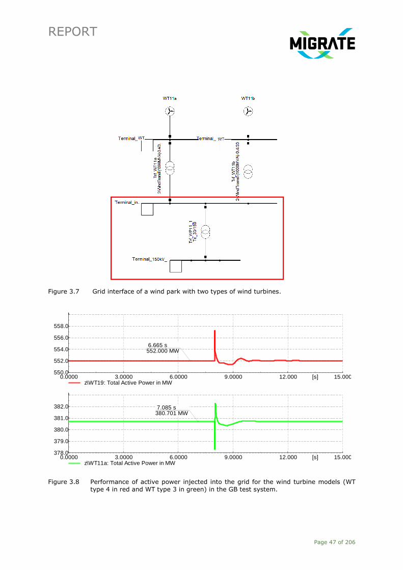
REPORT
Page 47 of 206
Figure 3.7 Grid interface of a wind park with two types of wind turbines.
Figure 3.8 Performance of active power injected into the grid for the wind turbine models (WT
type 4 in red and WT type 3 in green) in the GB test system.
15.00012.0009.00006.00003.00000.0000 [s]
382.0
381.0
380.0
379.0
378.0
z\WT11a: Total Active Power in MW
7.085 s380.701 MW
15.00012.0009.00006.00003.00000.0000 [s]
558.0
556.0
554.0
552.0
550.0
z\WT19: Total Active Power in MW
6.665 s552.000 MW
DIg
SIL
EN
T

REPORT
Page 48 of 206
The initialisation dynamic response of the both Type 3 and Type 4 wind turbine models during a
disturbance, integrated in GB system, is shown in Figure 3.8. The used GB system is the baseline
model in 2016 (see Section 3.3.2) and both tested wind turbines are located in zone 11 (Type 4)
and zone 19 (Type 3) of the GB system, i.e. North England and East England, respectively. The
upper plot of Figure 3.8 shows the active power response of the Type 3 wind turbine in zone 19
and the lower plot shows the active power response of the Type 4 wind turbine in zone 11. As it
can be seen, stable initialisation is achieved at t=4 seconds. In this simulation case, a generation
outage (2.2 GW) occurs at t=8s and stable output for both wind turbines is reached at t=12s. As
can be seen, the active power response is able to follow the power reference of the wind turbine.
Modelling in PSCAD
Controller Interactions are studied by implementing models for EMT simulations in PSCAD. Table
3.2 gives an overview of the selected elements in PSCAD for implementing the generic test case.
All these components are available in the Master Library of PSCAD. Additional libraries might be
required when simulating certain user specific models (such as the wind turbines discussed in the
next section). These libraries complement the Master Library.
Table 3.2 Power system modelling in PSCAD.
Element Details Reference
Voltage Source Three Phase Voltage Source Model 2
(Source Impedance Type: Ideal (R=0)
[31], [32]
Resistance
Inductance
Capacitance
Resistor
Inductor
Capacitor
A combination of these 3 elements can be used to
represent a very basic model of a transmission line
Two-winding transformer Three Phase 2 Winding Transformer
Transmission lines Bergeron Model (The Bergeron Model is a very
simple, constant frequency model based on
travelling waves)
Frequency Dependent Model (The Frequency
Dependent Model uses curve fitting to duplicate the
frequency response of a line or cable. It is the most
advanced time domain model available as it
represents the full frequency dependence of all line
parameters (including the effect of a frequency
dependent transform))
EMT Wind Turbine Models
For the MIGRATE project, Manitoba HVDC RC developed wind turbine type 3 and type 4 models.
This section gives a brief overview of those models. Within the EMT implementation two different

REPORT
Page 49 of 206
variations are provided. The complete model including the power electronic converters and an
average model, where the power electronic converters have been replaced with equivalent
voltage/current sources. These models are generic and most of its controls are based on the IEC
standards 61400-27-1 [26], [27]. Full details on these models as well as comparisons between the
two modelling techniques are presented for different realistic operating scenarios in [33].
DFIG Type 3 Model
The PSCAD generic DFIG model presented here has been setup for a single 3.6 MW machine
connected to a 50 Hz equivalent voltage source. A machine multiplier component can be used to
scale up the machine and thus simulate a collection of machines with only one wind generator, as it
is shown in Figure 3.9.
Figure 3.9 Single 3.6 MW DFIG connected to an equivalent voltage source through a 50x unit
multiplier.
The DFIG is an electromechanical system with electrical, mechanical and controls components. The
DFIG model is presented as a two-part system, with a mechanical subsystem, in charge of
converting the maximum power available from the wind into torque, and an electrical subsystem,
in charge of delivering such power into the electrical system (Figure 3.10). The interface
component in this system is the induction generator, which converts the mechanical energy into
electrical energy. The general parameters for the implemented DFIG model are presented in Table
3.3.
0.0602 [ohm] 0.001916
R=0
DFIGav
SCR 10X/R = 10
BRK
BRK
Dblk
x n
n
*
BRK
d/dt50.0
P = 180.4Q = 2.972V = 33.21
V
A

REPORT
Page 50 of 206
Figure 3.10 Electrical structure of DFIG electromechanical system.
Table 3.3 DFIG General Parameters.
Parameters Value
Cut in wind speed 3 m/s
Cut out wind speed 25 m/s
Nominal wind speed 10.2 m/s
Machine rating 4 MVA
Nominal frequency 50 Hz
Machine terminal voltage 0.9 kV
The initialisation of the detailed model is shown in Figure 3.11a. Stable operation is achieved at
t=5 seconds. In Figure 3.11b, the response of the detailed DFIG is shown for a 3-phase short
circuit of 150 milliseconds at the point of common coupling. The short circuit is applied at t=10
seconds; stable operation is achieved at t=20 seconds.
DFIG
Converters
Mechanical Model AC_sys
BRK#1
4.2 [MVA]
33/0.69/0.9
#3
#2
1000
V
A
*-1.0
V
A
S2TMODE
& Controls& Controls
GRID
ConverterConverter
GENERATOR
RABCSABC
S
TL
N
I M
W
CTRL
Istator
W0
WindTRQ
Wm
Vw
W0 Tm
Wind to torque
Pref
Ppu
Start
pu
Pitch
W0
W0
Wpu
V
A
VI_m
TurbStart
Signals
Pitch
Pg_pu
Two-Mass Model
Paero
TE w_WTR
wgenReset
W0
S2TMODE
A
B
Ctrl
Ctrl=1
T2ms
1
W0
T2ms
A
B
Ctrl
Ctrl=1
wWTR_Two_Mass
A
B
Ctrl
Ctrl = 1
WpuWpu_Mch
T2ms
Wpu
TE*
-1.0
Vwind_out
V
A

REPORT
Page 51 of 206
Figure 3.11 (a) initialisation of Detailed DFIG Model and (b) detailed DFIG Response to 150 ms 3-phase SC at the PCC.
Full Converter (Type 4) Model
The type-4 wind turbine is connected to an external electrical network (Figure 3.12) and can be
modified as required to represent a specific network situation.
Figure 3.12 Overview of the external network connection.
The type-4 wind turbine model is shown in Figure 3.13 and contains the following components:
─ Line Side and Machine Side Converters (LSC & MSC)
─ Converter dq Controllers (LSC & MSC)
─ Turbine Controller Modules (including emulated inertia and pitch angle control modules)
─ Multi-Mass Model
─ Two-Dimensional Aerodynamic Model
─ Wind turbine Transformer and Machine Models
Details of all the components can be found in [33].

REPORT
Page 52 of 206
Figure 3.13 Overview of the type-4 wind turbine module.
The general parameters for the implemented type-4 model are presented in Table 3.4 The
initialisation of the detailed model is shown in Figure 3.14. Stable operation is achieved at t=8 sec.
Table 3.4 Wind turbine T4 General Parameters.
Parameters Value
Cut in wind speed 3 m/s
Cut out wind speed 25 m/s
Nominal wind speed 10.2 m/s
Machine rating 6 MW
Nominal frequency 50 Hz
Machine terminal voltage 0.9 kV
Figure 3.14 Initialisation of Detailed Type 4 Model.

REPORT
Page 53 of 206
3.2.3 Generic Test Case 1: Frequency Performance in the Frequency
Containment Period
The PST16 Benchmark System
This generic test case was developed for the study of frequency performance in the frequency
containment period (i.e. the period after unbalance occurrence up to 30 seconds) and is based on
the PST16 benchmark system as described in [34], [35] and [36]. This system is suitable for
different kind of stability studies (frequency, rotor angle and voltage), as stated in [34].
Furthermore, the three interconnected areas in the system have weak connections because of the
length of the tie lines, which makes this system suitable for low-frequency oscillations studies as
well.
Figure 3.15 shows the diagram of the modified PST16 benchmark system as used in the MIGRATE
project. The grid consists of three strongly meshed areas, 66 buses, 16 generators, 28
transformers, and 51 transmission lines. Long transmission lines interconnect the areas (i.e.
200 km transmission lines). The loads are concentrated in area C and power is transferred from
area A and B to area C through two long tie-lines.
Figure 3.15 Modified PST16 benchmark system.
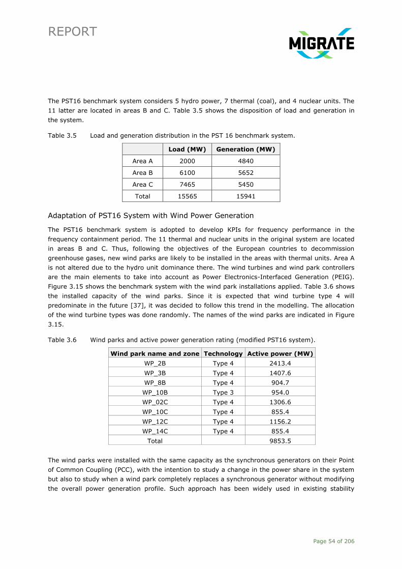
REPORT
Page 54 of 206
The PST16 benchmark system considers 5 hydro power, 7 thermal (coal), and 4 nuclear units. The
11 latter are located in areas B and C. Table 3.5 shows the disposition of load and generation in
the system.
Table 3.5 Load and generation distribution in the PST 16 benchmark system.
Load (MW) Generation (MW)
Area A 2000 4840
Area B 6100 5652
Area C 7465 5450
Total 15565 15941
Adaptation of PST16 System with Wind Power Generation
The PST16 benchmark system is adopted to develop KPIs for frequency performance in the
frequency containment period. The 11 thermal and nuclear units in the original system are located
in areas B and C. Thus, following the objectives of the European countries to decommission
greenhouse gases, new wind parks are likely to be installed in the areas with thermal units. Area A
is not altered due to the hydro unit dominance there. The wind turbines and wind park controllers
are the main elements to take into account as Power Electronics-Interfaced Generation (PEIG).
Figure 3.15 shows the benchmark system with the wind park installations applied. Table 3.6 shows
the installed capacity of the wind parks. Since it is expected that wind turbine type 4 will
predominate in the future [37], it was decided to follow this trend in the modelling. The allocation
of the wind turbine types was done randomly. The names of the wind parks are indicated in Figure
3.15.
Table 3.6 Wind parks and active power generation rating (modified PST16 system).
Wind park name and zone Technology Active power (MW)
WP_2B Type 4 2413.4
WP_3B Type 4 1407.6
WP_8B Type 4 904.7
WP_10B Type 3 954.0
WP_02C Type 4 1306.6
WP_10C Type 4 855.4
WP_12C Type 4 1156.2
WP_14C Type 4 855.4
Total 9853.5
The wind parks were installed with the same capacity as the synchronous generators on their Point
of Common Coupling (PCC), with the intention to study a change in the power share in the system
but also to study when a wind park completely replaces a synchronous generator without modifying
the overall power generation profile. Such approach has been widely used in existing stability
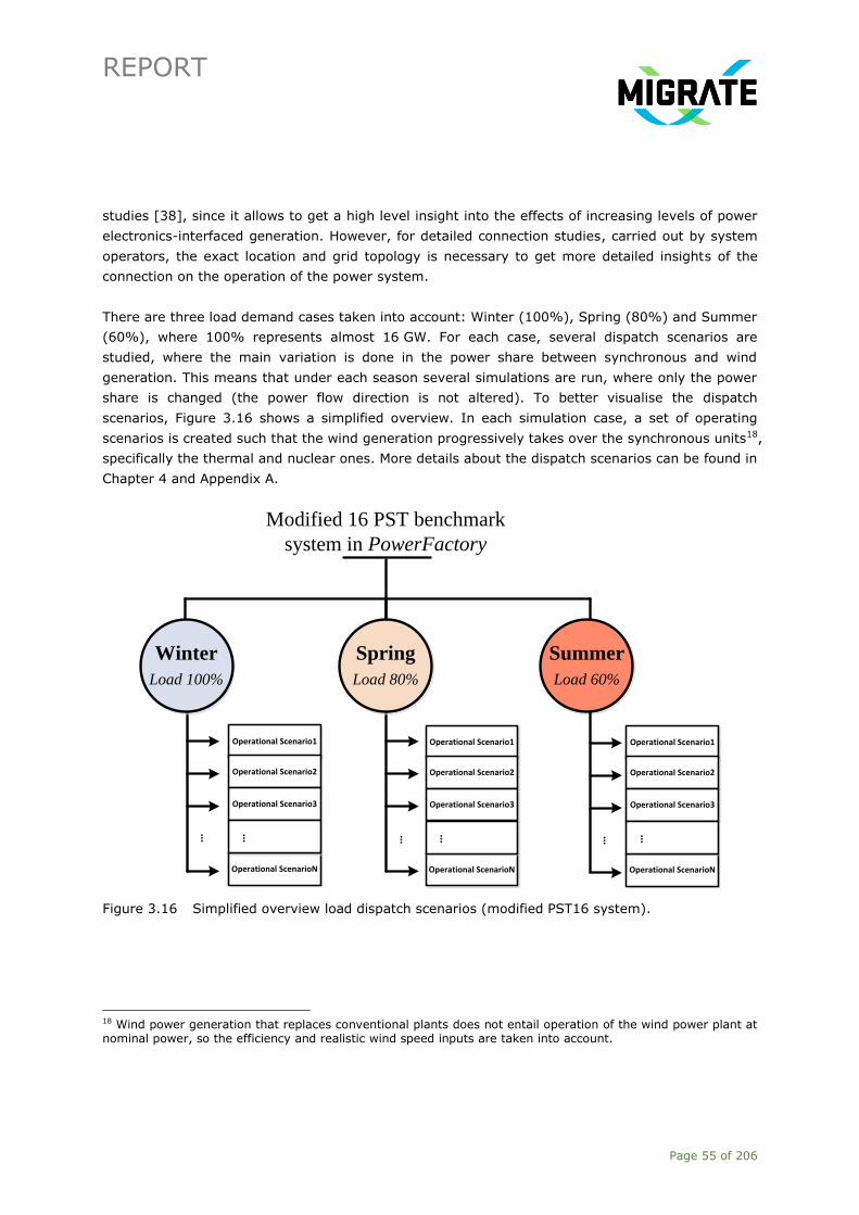
REPORT
Page 55 of 206
studies [38], since it allows to get a high level insight into the effects of increasing levels of power
electronics-interfaced generation. However, for detailed connection studies, carried out by system
operators, the exact location and grid topology is necessary to get more detailed insights of the
connection on the operation of the power system.
There are three load demand cases taken into account: Winter (100%), Spring (80%) and Summer
(60%), where 100% represents almost 16 GW. For each case, several dispatch scenarios are
studied, where the main variation is done in the power share between synchronous and wind
generation. This means that under each season several simulations are run, where only the power
share is changed (the power flow direction is not altered). To better visualise the dispatch
scenarios, Figure 3.16 shows a simplified overview. In each simulation case, a set of operating
scenarios is created such that the wind generation progressively takes over the synchronous units18,
specifically the thermal and nuclear ones. More details about the dispatch scenarios can be found in
Chapter 4 and Appendix A.
Summer
Load 60%
Operational Scenario1
...
...
...
Spring
Load 80%
Winter
Load 100%
Modified 16 PST benchmark
system in PowerFactory
Operational Scenario2
Operational Scenario3
Operational ScenarioN
...
Operational Scenario1
Operational Scenario2
Operational Scenario3
Operational ScenarioN
...
Operational Scenario1
Operational Scenario2
Operational Scenario3
Operational ScenarioN
...
Figure 3.16 Simplified overview load dispatch scenarios (modified PST16 system).
18 Wind power generation that replaces conventional plants does not entail operation of the wind power plant at nominal power, so the efficiency and realistic wind speed inputs are taken into account.

REPORT
Page 56 of 206
Description of Operating Conditions
The case study describes the operating conditions under which conditions of instability can occur. A
heuristic approach is followed to stress the test system such that insight on the hazards can be
revealed. This approach will make a complete scan on the system behaviour. The methodology
followed runs a large amount of simulations with different power share from PEIG with three
different load demand profiles, corresponding to winter, spring and summer time. The objective is
to perform a sensitivity analysis, which will contribute to understand the possible sources of
frequency instability for high penetration of renewables.
For a more detailed discussion of the approach for the development of load scenarios and operating
conditions, it is referred to Appendix A.
It was considered to perform the simulations under the following circumstances:
─ No change in topology.
─ Line out-of-service. The tie-line selected to be out-of-service is the one connecting area A with
area C (tie line A-C in Figure 3.15) as it was found that this is the worst case scenario.
Besides the different grid topologies and power dispatch, the RMS simulations are performed by
setting a power imbalance of 6.3% and 13%. This is achieved by tripping the following generators:
─ A1aG and A1bG
─ A2aG and A2bG
─ A1aG or A1bG or A2aG or A2bG (one at a time).
No short circuits, line outages or any other types of events are considered because the normative
contingency for interconnected operation in continental Europe is the tripping of two of the largest
generating facilities connected to the same busbar (for frequency studies) [39].
3.2.4 Generic Test Case 2: Large-Disturbance Rotor Angle Stability and Small-
Disturbance Voltage Stability
The IEEE 9-bus system [40], which is well known as the P.M. Anderson 9-bus model, is used to
assess the large-disturbance rotor angle stability and small-disturbance voltage stability of RES-
dominated power systems. The system consists of 3 synchronous generators with IEEE type 1
exciters, 6 transmission lines, and 3 constant impedance loads. Small modifications are made to
make this test system suitable for studying these two stability phenomena.
Large-Disturbance Rotor Angle Stability
For Large-Disturbance rotor angle stability, the modified 9-bus test system is shown in Figure 3.17.
As shown in the single line diagram, generator G1 is replaced by a wind turbine type 3. In the rotor
angle stability studies, G3 is selected as the reference generator. The angle of generator G2 is
observed to investigate large-disturbance rotor angle stability. The system steady-state (initial
conditions) information is provided in Table 3.7.
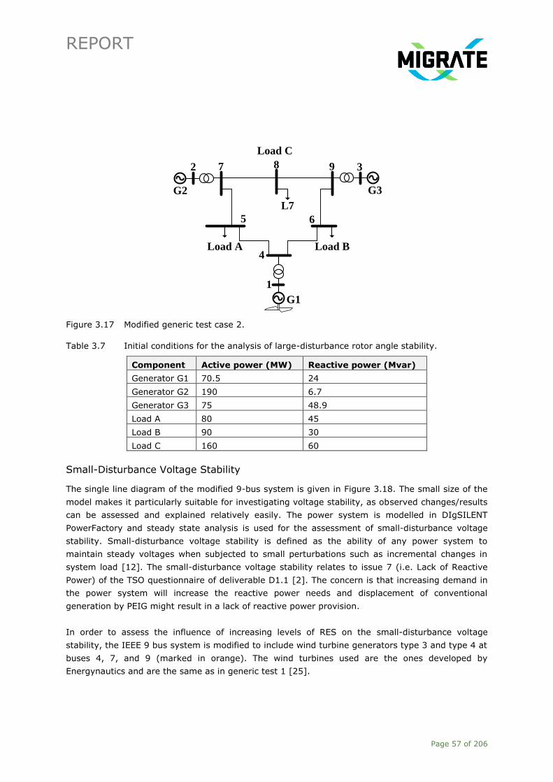
REPORT
Page 57 of 206
G3
2
G2
G1
3
1
5
4
987
6
L7
Load A
Load C
Load B
Figure 3.17 Modified generic test case 2.
Table 3.7 Initial conditions for the analysis of large-disturbance rotor angle stability.
Component Active power (MW) Reactive power (Mvar)
Generator G1 70.5 24
Generator G2 190 6.7
Generator G3 75 48.9
Load A 80 45
Load B 90 30
Load C 160 60
Small-Disturbance Voltage Stability
The single line diagram of the modified 9-bus system is given in Figure 3.18. The small size of the
model makes it particularly suitable for investigating voltage stability, as observed changes/results
can be assessed and explained relatively easily. The power system is modelled in DIgSILENT
PowerFactory and steady state analysis is used for the assessment of small-disturbance voltage
stability. Small-disturbance voltage stability is defined as the ability of any power system to
maintain steady voltages when subjected to small perturbations such as incremental changes in
system load [12]. The small-disturbance voltage stability relates to issue 7 (i.e. Lack of Reactive
Power) of the TSO questionnaire of deliverable D1.1 [2]. The concern is that increasing demand in
the power system will increase the reactive power needs and displacement of conventional
generation by PEIG might result in a lack of reactive power provision.
In order to assess the influence of increasing levels of RES on the small-disturbance voltage
stability, the IEEE 9 bus system is modified to include wind turbine generators type 3 and type 4 at
buses 4, 7, and 9 (marked in orange). The wind turbines used are the ones developed by
Energynautics and are the same as in generic test 1 [25].
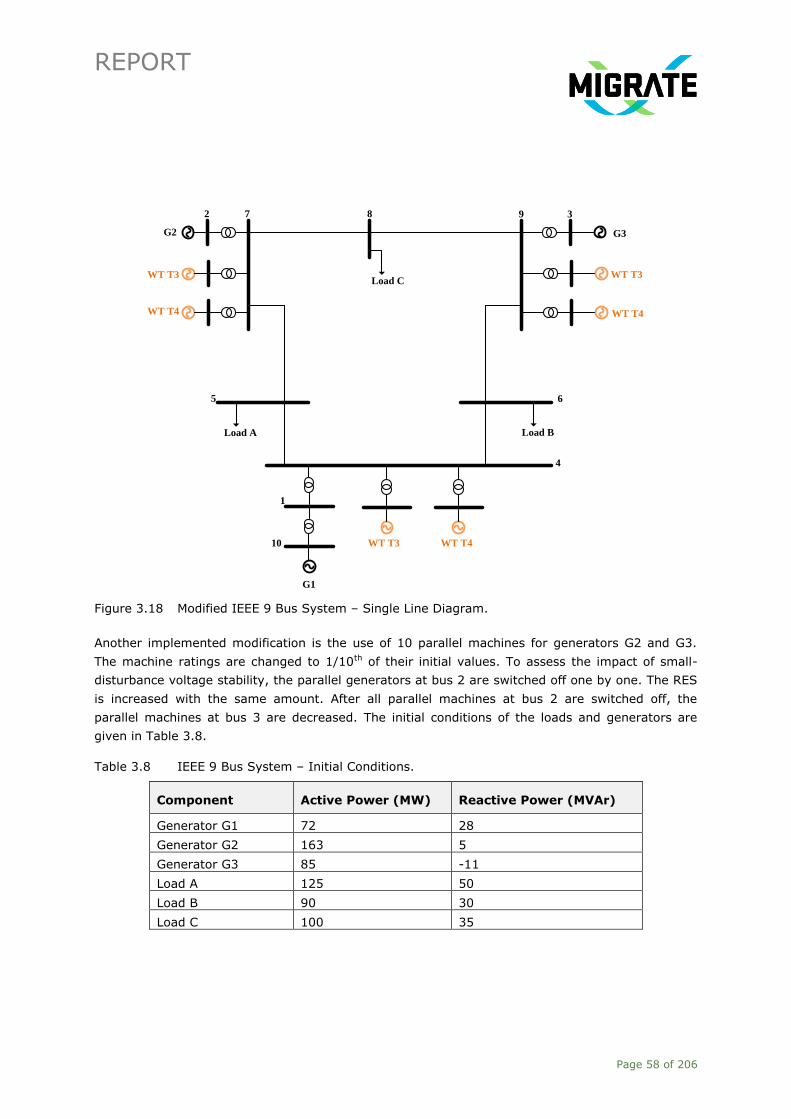
REPORT
Page 58 of 206
Figure 3.18 Modified IEEE 9 Bus System – Single Line Diagram.
Another implemented modification is the use of 10 parallel machines for generators G2 and G3.
The machine ratings are changed to 1/10th of their initial values. To assess the impact of small-
disturbance voltage stability, the parallel generators at bus 2 are switched off one by one. The RES
is increased with the same amount. After all parallel machines at bus 2 are switched off, the
parallel machines at bus 3 are decreased. The initial conditions of the loads and generators are
given in Table 3.8.
Table 3.8 IEEE 9 Bus System – Initial Conditions.
Component Active Power (MW) Reactive Power (MVAr)
Generator G1 72 28
Generator G2 163 5
Generator G3 85 -11
Load A 125 50
Load B 90 30
Load C 100 35
G1
1
10
Load A
5
G2
72 8
Load C
Load B
G3
9 3
6
4
WT T3
WT T4
WT T3
WT T3
WT T4
WT T4

REPORT
Page 59 of 206
3.2.5 Generic Test Case 3: Sub-synchronous Controller Interactions
A series compensated overhead line can produce oscillations in the sub-synchronous frequency
range. When this overhead line is electrically close to a PEID (mainly WT T3), these oscillations can
grow if the damping of the system is not large enough. This can occur when the PEID exhibits a
negative resistance behaviour in which the negative resistance is larger than the positive resistance
of the network. This interaction between the PEID and the series compensated line is defined as
Sub-Synchronous Controller Interaction (SSCI). As no mechanical devices are involved in the
resonance, this phenomenon is a purely electrical oscillation. Due to this nature oscillations can
grow substantially in a short time.
The generic test case for Sub-Synchronous Controller Interactions (SSCI) is based on the IEEE First
Benchmark Model for Sub-Synchronous Resonance (SSR) [41] and is shown in Figure 3.19. This
generic test case is used to get basic insight into the parameters that influence the SSCI
occurrence.
Figure 3.19 Generic Test Case SSCI – Single Line Diagram.
More elaborated simulations are carried out using the model of Figure 3.20, in which more wind
turbines are present. The model of Figure 3.20 uses parallel network interfaces to enable
acceptable simulation times. Therefore, the connections of the lines ‘TLine_1’ to ‘TLine_3’ go to
three separate cases containing detailed wind turbine models. The values of the RLC components
can be altered with the aim of achieving a certain network behaviour (e.g. damping or a specific
level of series compensation). An EMT environment is necessary for investigating the controller
interactions, as an RMS environment cannot model the devices in enough detail. An RMS based
software is not capable of illustrating correct sub synchronous or harmonic phenomena due to
modelling simplifications. As the EMT wind models provided by Manitoba HVDC RC are developed in
PSCAD, the generic test case is modelled using PSCAD/EMTDC, with a solution time step of 25 µs.
0.0602 [ohm] 0.001916
R=0
SCR 10X/R = 10
DFIGPCC
1.0 [uF]

REPORT
Page 60 of 206
Figure 3.20 Extended Model for SSCI – Single Line Diagram.
3.3 Development of Realistic Test Cases of Medium Size
After using the Generic Test Cases described in Section 3.2 for the development and initial testing
of the power system analysis methodologies laid out in Chapter 4, the adapted methodologies are
applied to more realistic, medium-sized power grids along with realistic Transition Scenarios for the
migration from the status quo to a PE dominated power system. These Realistic Test Cases are
based on the GB and the Irish test system.
3.3.1 Development of Transition Scenarios
What is a Transition?
A transition is defined as ‘a change from one form or type to another, or the process by which this
happens’ [43]. Within the MIGRATE project, transition scenarios are used to describe the changes
in the electricity landscape over time, i.e. increasing levels of installed Power Electronics-Interfaced
Generation (PEIG). The aim is to assess the impact of these changes in the transmission grid.
Transitions have 5 main characteristics [44]:
1. A transition is a co-evolution process:
This is a process in which some domains continuously adapt to and influence each other, leading
to interdependencies. As an illustration, one can examine the influence of environmental policies
on the generation segment.
2. A transition is a multi-actor process:
At least 2 domains, with different actors, are required in a transition. Within the electricity
transition, several actors are involved, e.g. policy makers, manufacturers, generators,
consumers, transmission system operators, etc.
3. A transition is a radical shift from one system to another:
Radical here refers to the scope of the shift, rather than its speed. The shift may be sudden,
slow, or in a step-wise fashion. In the example of an electricity transition, the shift is from a
conventional generation dominated system to a PE dominated power system.
0.0602 [ohm] 0.001916
fR=0
SCR 10X/R = 10
Freq_sys
d/dt
TLin
e_1
TLine_1
12 to
4
5
1WPre
f
BRKn
Punit_
base
Punit_
base
BRKn
WPre
f
1
12 to
4
5
TLine_2
TLin
e_2
TLin
e_3
TLine_3
1
2 t
o 4 5
1
WPre
f
BRKn
Punit_base
1.0 [uF]

REPORT
Page 61 of 206
4. A transition is a long-term process:
A time frame of 30-50 years is generally considered. This interval takes into account the time
required for the breakthrough of innovations, as well as for making these innovations embedded
in the system.
5. A transition is macroscopic:
Because transitions have a co-evolution and multi-actor nature, it affects several domains.
Therefore it is macroscopic. With decreasing levels of conventional generators, the electricity
network will be operated differently (e.g. operational limits based on stability instead of thermal
capacity, new ancillary services), energy will be traded differently (e.g. renewable energy feed-
in tariffs), etc.
A transition is, qualitatively, usually depicted using the S-curve as shown in Figure 3.21. The x-axis
contains the time, whereas the y-axis contains some sort of indicator for the change in the system.
As an example the installed PE-based generation is chosen as indicator for system change in the
picture below.
Figure 3.21 The S-curve model of transitions.
In the S-curve, 4 stages can be observed:
─ Predevelopment: in this stage innovations are being developed; the status quo does not change
visibly.
─ Take-off: innovations are already developed in this stage; the state of the art starts to change.
─ Acceleration: innovations are being embedded in the system; the system is undergoing a
paradigm shift.
─ Stabilisation: the speed of the system change (i.e. installed PE in the graph) decreases and a
new equilibrium is reached; the system successfully adapted to the change.
It should be noted that the S-curve is not a fixed pathway and that the phases are only conceptual:
the S-curve cannot be used to predict the specific course of transitions.

REPORT
Page 62 of 206
Use of Transition in MIGRATE
One of the main objectives for this task of the project is to develop and use a small set of generic
test cases able to grasp system stability issues raised by the growing power electronic connection
into any given zone. However, the results of the generic test cases should be compared with the
expected situation in Ireland and Great Britain (GB). These comparisons will be provided as a
validation of relevant model characteristics as the analysis of angular and frequency stability
challenges [1]. The mentioned "expected situations", or scenarios, must represent a transition
between current situation of the transmission system and expected situation in the future.
The transition scenarios are a set of models where the expected installed generation capacity (i.e.
conventional and PEIG), load demand, power flows and possible grid reinforcements for the years
2016, 2020, 2025, 2030, and 2035, are configured in a reduced model of the Great Britain (GB)
system. These scenarios were built upon an original GB reduced model. Such original model was
built considering a scenario for the year 2013, thus it was upgraded using the information available
in “UK electricity transmission, Electricity Ten Year Statement 2016” by National Grid [45], [46].
The main objective of these scenarios is to be used as validation systems to assess the impact of
increasing levels of PE penetration in the transmission grid.
Proposed Framework
In the framework described next, it is proposed to analyse the transition of the electricity system
using 3 underlying transitions:
1. Network transition (N)
For this transition, the focus is on development in network topologies and the increased use of
PE-based devices for the network such as HVDC and STATCOMs. The assumption is that the
network development will face the slowest transition because of the very long lead times (as a
result of public opposition, technical challenges, regulatory requirements, etc.) involved in
realising such projects.
2. Generation transition (G)
The focus here is the transition from conventional, synchronous machine-based generation to
more PE-dominated generation (wind parks and PV parks). The assumption is that this
transition will be the fastest as a result of subsidy schemes for RES and because of the fact that
the generation is an open market segment. One important parameter is the fraction of PEIG
that is connected to the transmission grid (vs. the distribution grid)
3. Load transition (L)
This transition deals with how the load will evolve throughout time. A moderate transition speed
is expected. It is expected that the load increase will not be proportional to the increase in
population, because of energy efficiency measures in (domestic) appliances. Two important
parameters here are the load profile and the load composition.

REPORT
Page 63 of 206
3.3.2 Implementation into the GB Test System
Implementation of the Transition Scenarios
For the implementation of the transition scenarios in the Great Britain (GB) power system,
information on the 3 types of transitions defined above is gathered. For future network
development, the publication Network Options Assessment by National Grid [45] has been used as
inspiration. For the transition in generation, the Electricity Ten Year Statement [46] and Scenario
Outlook and Adequacy Forecast 2015 [47] were used. The Future Energy Scenarios document by
National Grid [48] was used to obtain an overall overview of the developments in GB.
The detailed GB power system is too complex and too big to be used in repetitive time domain
simulations. A fully represented system would have hundreds of substations with highly detailed
transmission line modelling, such that for performing the analysis defining boundaries is very
important. A boundary "splits the entire (Great Britain) system into adjacent parts, crossing critical
circuit paths that carry power between the areas where power flow limitations may be
encountered" [46]. There are at least 20 reported boundaries in the current GB transmission
system.
To reduce the complexity of the system, a dynamic equivalent with reduced number of variables
must be defined such that some simplifications are made. There is no computational overburden
and the dynamic response of the reduced model resembles the full GB system in a way that the
analysis of results can be comparable to that of the full system. This way, the use of the so-called
reduced model can provide great advantages for the study of the concepts of interests while
intending them to be used in the GB system.
In [49], L. Shen from University of Manchester has developed a reduced model based on steady-
state data provided by the University of Strathclyde which was validated against a solved AC power
flow reference case provided by National Grid Electricity Transmissions. The main structure of the
network is shown in Figure 3.22, where each of the 29 substations represents a grouped level of
generation, load demand and losses.
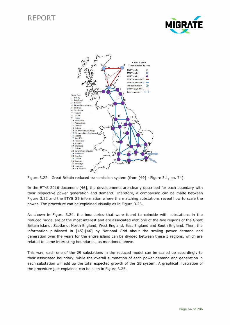
REPORT
Page 64 of 206
Figure 3.22 Great Britain reduced transmission system (from [49] - Figure 3.1, pp. 74).
In the ETYS 2016 document [46], the developments are clearly described for each boundary with
their respective power generation and demand. Therefore, a comparison can be made between
Figure 3.22 and the ETYS GB information where the matching substations reveal how to scale the
power. The procedure can be explained visually as in Figure 3.23.
As shown in Figure 3.24, the boundaries that were found to coincide with substations in the
reduced model are of the most interest and are associated with one of the five regions of the Great
Britain island: Scotland, North England, West England, East England and South England. Then, the
information published in [45]-[46] by National Grid about the scaling power demand and
generation over the years for the entire island can be divided between these 5 regions, which are
related to some interesting boundaries, as mentioned above.
This way, each one of the 29 substations in the reduced model can be scaled up accordingly to
their associated boundary, while the overall summation of each power demand and generation in
each substation will add up the total expected growth of the GB system. A graphical illustration of
the procedure just explained can be seen in Figure 3.25.

REPORT
Page 65 of 206
Figure 3.23 Overview of matching process with the work flow.
Figure 3.24 Mapping of the 5 ETYS regions onto the 29 zone network model.

REPORT
Page 66 of 206
Figure 3.25 Steps to relate the National Grid information with the existing reduced GB model.
Step four of Figure 3.25, "Estimate generation dispatch", was done by following two principles:
1. Power Electronics-Interfaced Generation (only wind turbines considered in this work) have
priority over synchronous generation due to environmental and economic reasons.
2. The power flow direction was kept at all times, i.e. from north to south and from east to west
(when applicable), see also Appendix B.1.
To accomplish a proper dispatch profile, the generation dispatch at northern regions was kept
bigger than the load demanded locally, while at southern substations the generation was kept
significantly below the demanded power.
For the implementation of the transition scenario in the GB system, it was chosen to select the two
extremes, i.e. Gone Green (GG) and No Progression (NP), in order to study the worst case
scenarios. The Gone Green scenario is based on the assumption that all renewable generation and
environmental targets are achieved: 15% of all energy from RES by 2020, and 80% reduction in
greenhouse gasses by 2050. The No Progression scenario is based on the assumption that only
new units that are already under construction, or too far advanced to be cancelled, are
commissioned. Figure 3.26 shows the development of the conventional generation and the Power
Electronics-Interfaced Generation (PEIG) over time for the Gone Green and No Progression
scenarios. In Appendix B.1, more details can be found regarding the division over the 29 zones in
the reduced GB model.
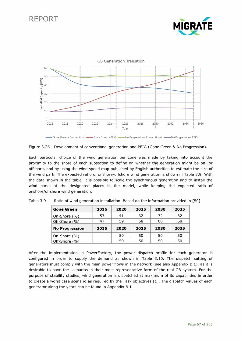
REPORT
Page 67 of 206
Figure 3.26 Development of conventional generation and PEIG (Gone Green & No Progression).
Each particular choice of the wind generation per zone was made by taking into account the
proximity to the shore of each substation to define on whether the generation might be on- or
offshore, and by using the wind speed map published by English authorities to estimate the size of
the wind park. The expected ratio of onshore/offshore wind generation is shown in Table 3.9. With
the data shown in the table, it is possible to scale the synchronous generation and to install the
wind parks at the designated places in the model, while keeping the expected ratio of
onshore/offshore wind generation.
Table 3.9 Ratio of wind generation installation. Based on the information provided in [50].
Gone Green 2016 2020 2025 2030 2035
On-Shore (%) 53 41 32 32 32
Off-Shore (%) 47 59 68 68 68
No Progression 2016 2020 2025 2030 2035
On-Shore (%) 50 50 50 50
Off-Shore (%) 50 50 50 50
After the implementation in PowerFactory, the power dispatch profile for each generator is
configured in order to supply the demand as shown in Table 3.10. The dispatch setting of
generators must comply with the main power flows in the network (see also Appendix B.1), as it is
desirable to have the scenarios in their most representative form of the real GB system. For the
purpose of stability studies, wind generation is dispatched at maximum of its capabilities in order
to create a worst case scenario as required by the Task objectives [1]. The dispatch values of each
generator along the years can be found in Appendix B.1.

REPORT
Page 68 of 206
Table 3.10 Total load demand in the GB system over the years.
2016 2020 2025 2030 2035
Gone Green [GW] 52.450 48.749 49.349 52.900 57.050
No Progression [GW] 52.450 49.249 46.850 44.850 44.949
The scaling of generation and demand causes the need to reinforce the grid capabilities either in
topology (new lines, capacitors, STATCOMS, etc.) or in rated capacity of the existing elements. To
do so the NOA document [45] was consulted and used as inspiration to apply any required
reinforcement. The word “inspiration” is crucial to understand the use of the mentioned document
because in the frame of this research, it is nearly impossible to execute the actions mentioned
there because it is too detailed about real existing lines or equipment, which means it mentions
elements or zones that are not represented in the reduced model.
The way to proceed is to implement the scaling in generation and demand, and to analyse the
required reinforcements in the GB model afterwards. Once this is done, a double check of those
required activities is contrasted with the NOA study to corroborate the similarity in nature (i.e. in
NOA also similar actions are executed, although maybe not in the same region or substation).
Implementation in PowerFactory
The model of the GB system in PowerFactory is a reduced model, which consists of five areas:
Scotland, North England, West England, East England and South England [51]. The model is
organised into 29 zones, each one comprising one bus, one conventional power plant represent the
dominant type of generation in the zone, and a load. The generators are represented by using the
sixth order model, whereas the loads are represented with the static ZIP model, which is set to
work as a constant power model (worst case). The buses are interconnected through 99
transmission lines (49 double-circuit lines, and one single-circuit line). These transmission lines
represent the main routes for the power flows across the GB system.
In the reduced model of the GB system, each substation is constructed based on the topology
shown in Figure 3.27. All the elements connected to the node bus have representative values, i.e.
they are grouped elements that include others that were not represented in the network. In this
way, the generators and loads have larger ratings than normal commercial generators or single
loads. The load models used in the GB system are 100% static loads, modelled as constant power
loads (both P and Q). The parameters of the ZIP model in PowerFactory were taken from [52].
The transition scenarios are a set of 9 PowerFactory files (pfd extension files) as shown in Figure
3.28, shared with the MIGRATE consortium under the internal communication memo "Great Britain
transition scenarios in DIgSILENT - PowerFactory" on 07-04-2017.

REPORT
Page 69 of 206
Figure 3.27 Node bus structure in the reduced GB system (from [49] - Figure 3.2, pp. 76).
The procedure for developing the baseline scenario (year 2016), similarly to all the other cases,
starts by setting the installed capacity of the synchronous machines and wind generation. This is
done by changing the number of parallel machines or the rating capabilities of the type model,
while for the latter the information of onshore/offshore installation is of major relevance because
the offshore wind parks have different topology than the onshore ones.
The dispatched generation and load demand is implemented in PowerFactory after determining the
installed capacity (as shown in the tables in B.1). Subsequently, a power flow calculations is
executed to perform an element inspection where the overloaded parts or buses with undesired
voltage deviations are identified, so the necessary corrective actions (reactive power
compensation) can be taken. Figure 3.29 shows the procedure used for the creation of the baseline
scenario, and the transition scenarios.
Figure 3.28 PowerFactory Data manager with the 9 transition scenarios archives.
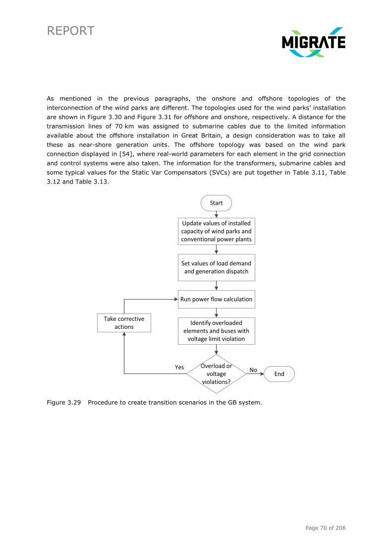
REPORT
Page 70 of 206
As mentioned in the previous paragraphs, the onshore and offshore topologies of the
interconnection of the wind parks are different. The topologies used for the wind parks’ installation
are shown in Figure 3.30 and Figure 3.31 for offshore and onshore, respectively. A distance for the
transmission lines of 70 km was assigned to submarine cables due to the limited information
available about the offshore installation in Great Britain, a design consideration was to take all
these as near-shore generation units. The offshore topology was based on the wind park
connection displayed in [54], where real-world parameters for each element in the grid connection
and control systems were also taken. The information for the transformers, submarine cables and
some typical values for the Static Var Compensators (SVCs) are put together in Table 3.11, Table
3.12 and Table 3.13.
Start
Update values of installed capacity of wind parks and conventional power plants
Set values of load demand and generation dispatch
Run power flow calculation
Identify overloaded elements and buses with
voltage limit violation
Overload or voltage
violations?End
Take corrective actions
Yes No
Figure 3.29 Procedure to create transition scenarios in the GB system.

REPORT
Page 71 of 206
Figure 3.30 Connection of offshore wind park to the grid.
Table 3.11 Line data for offshore wind park connection.
Component Impedance Capacitance
150 kV sub.cable 0.046+j0.113 Ω/km 241.0 nF/km
Table 3.12 Transformer data for offshore wind park connection.
Transformer type Voltage Rated power Impedance
Wind turbine trafo (for Type 4 turbines) 0.4/33 kV 1000 MVA 0.06
Wind turbine trafo (for Type 3 turbines) 0.66/33 kV 1000 MVA 0.06
Table 3.13 SVS data (biggest value) for offshore wind park connection.
Q Reactance (>0) Mvar = 1121 Q per Capacitor unit (<0) Mvar = -337.12
The SVSs described in Table 3.13 are meant to compensate the charging reactive power of the
cables, and thus, to minimise the steady state voltage deviation from bus bars at 150 kV. The
number of parallel cables displayed in the offshore schematic depends on the power level to be
transmitted, since to the cables used in this work have fixed ampacities of either of 2 or 2.66 kA.
Figure 3.31 Connection of onshore wind park to the grid.
On the other hand, Figure 3.32 shows a schematic of the way of connection of all the synchronous
generators, as it was defined by the researchers of the University of Manchester in [49].
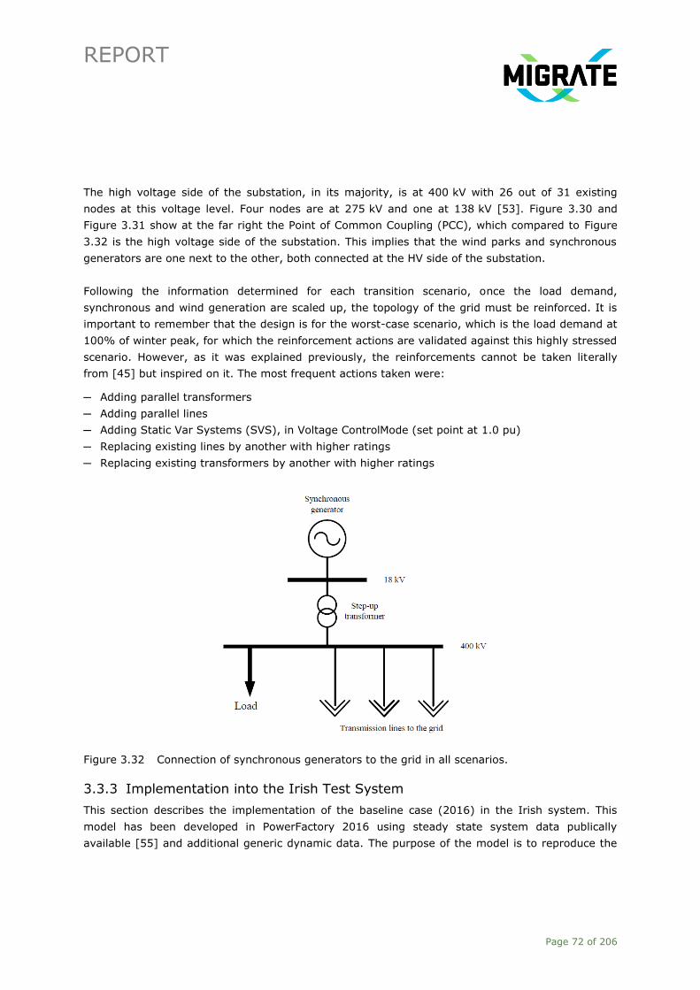
REPORT
Page 72 of 206
The high voltage side of the substation, in its majority, is at 400 kV with 26 out of 31 existing
nodes at this voltage level. Four nodes are at 275 kV and one at 138 kV [53]. Figure 3.30 and
Figure 3.31 show at the far right the Point of Common Coupling (PCC), which compared to Figure
3.32 is the high voltage side of the substation. This implies that the wind parks and synchronous
generators are one next to the other, both connected at the HV side of the substation.
Following the information determined for each transition scenario, once the load demand,
synchronous and wind generation are scaled up, the topology of the grid must be reinforced. It is
important to remember that the design is for the worst-case scenario, which is the load demand at
100% of winter peak, for which the reinforcement actions are validated against this highly stressed
scenario. However, as it was explained previously, the reinforcements cannot be taken literally
from [45] but inspired on it. The most frequent actions taken were:
─ Adding parallel transformers
─ Adding parallel lines
─ Adding Static Var Systems (SVS), in Voltage ControlMode (set point at 1.0 pu)
─ Replacing existing lines by another with higher ratings
─ Replacing existing transformers by another with higher ratings
Figure 3.32 Connection of synchronous generators to the grid in all scenarios.
3.3.3 Implementation into the Irish Test System
This section describes the implementation of the baseline case (2016) in the Irish system. This
model has been developed in PowerFactory 2016 using steady state system data publically
available [55] and additional generic dynamic data. The purpose of the model is to reproduce the

REPORT
Page 73 of 206
stability problems identified with the generic test cases (in Section 3.2) and to facilitate detailed
investigations of the dynamic behaviour in a real system. In no way should this model be
interpreted as a true representation of the Irish power system at any particular point in time or
should be used for the purposes of replicating specific events in the grid. While accurate, many
simplifications had to be made for technical and commercial reasons. Therefore, the results
produced with this model will give a typical and meaningful (rather than exact) picture of the
performance of a small isolated system with large share of PE based generation, like in Ireland.
Current Situation
The Ireland and Northern Ireland power system is a synchronous island system with limited HVDC
interconnection to Great Britain. This single synchronous power system has a forecasted peak
demand of approximately 7000 MW and an expected installed capacity of dispatchable conventional
generation of 9500 MW by 2020.
European legislation has mandated that at least 20% of the European Union’s final energy
consumption should come from renewable energy by 2020. In Ireland, the electricity sector has
been mandated to deliver the majority of this renewable energy contribution and has set an
electrical energy target of 40% from renewable resources by 2020. Wind power will be the
dominant resource in meeting the targets with approximately 37%.
The transmission system in Ireland is operated at 400 kV, 220 kV and 110 kV. The transmission
system in Northern Ireland is operated at 275 kV and 110 kV. The two transmission systems are
connected by means of one 275 kV double circuit. The 400 kV, 275 kV and 220 kV networks form
the backbone of the all-island transmission system. Typically large generation stations (greater
than 100 MW) are connected to the 220 kV, 275 kV or 400 kV networks. The 110 kV circuits
provide parallel paths to the 220 kV, 275 kV and 400 kV networks and are the most extensive
elements of the all-island transmission system.
The transmission system is generally comprised of overhead lines. There are exceptions to this,
such as in the city centres of Belfast, Cork and Dublin, where underground cables are exclusively
used. Moreover, increasing amounts of underground cables are being installed in remote areas
(such as the South West) to facilitate connections of wind farms to the nearest grid infrastructure.
The East West HVDC Interconnector links the electricity grids in Ireland and Wales, while the Moyle
HVDC Interconnector links the electricity grids in Northern Ireland and Scotland. Figure 3.33 shows
a geographical map of the existing transmission grid at the beginning of July 2016.

REPORT
Page 74 of 206
Figure 3.33 All Island Transmission System (July 2016) [55].
Northern
Ireland
KILTOY
CATHALEEN'S
FALL
BINBANE
DRUMKEEN
MEENTYCAT
SORNE
HILL
TRILLICK
DRYBRIDGE
LOUTH
MEATH
HILL
MULLAGHARLIN
NAVAN
SLIGO
TAWNAGHMORE
MOY
CASTLEBAR
RICHMOND
CARRICK
- ON -
SHANNON
BELLACORICK
GILRA
ARIGNA
TONROE
CORRACLASSY
CUNGHILL
CORDERRY
FLAGFORD
GARVAGH
SHANKILL
ARVA
RATRUSSAN
ENNIS
DALLOW
PORTLAOISE
CRANE
CARLOW
KILKENNY
THURLES
CAHIR
DOON
ANNER
BALLYDINE
MALLOW
CHARLEVILLE
RATHKEALE
TARBERT
BUTLERSTOWN
DUNGARVAN
BLAKE
TULLABRACK
MUNGRET
MONETEEN
FASSAROE
POLLAPHUCA
IKERRIN
LISHEEN
OUGHTRAGH
TRALEE
DUNFIRTH
KILLOTERAN
KILLONAN
STRATFORD
BALLYBEG
TIPPERARY
GLENLARA
ATHY
PROSPECT
MONREAD
TRIEN
AHANE
ARDNACRUSHA
LIMERICK
CASTLEFARM
SEALROCK
WATERFORD
TYNAGH
SINGLAND
CLAHANE
DERRYBRIEN
AGANNYGAL
AUGHINISH
WEXFORD
KILTEEL
BALLYWATER
GREAT
ISLAND
CULLENAGH
TURLOUGH
HILL
CARRICKMINES
SEE
DUBLIN
AREA
NORTH WALL
SHELLYBANKSIRISHTOWN
OLDSTREET
FINGLAS
BARODA
NEWBRIDGE
HUNTSTOWN
MONEYPOINT
KELLIS
ARKLOW
PLATIN
KNOCKUMBER
GORMAN
BALTRASNA
GLASMORECORDUFF
WOODLAND
ATHLONE
CASHLA
GALWAY
LANESBORO
THORNSBERRY
CLOON
SOMERSET
CUSHALING
DALTON
SALTHILL
DERRYIRON
SHANNONBRIDGE
KINNEGAD
MULLINGAR
BANDON
DUNMANWAY
MACROOM
BRINNY
KNOCKRAHAKILBARRY
RAFFEENAGHADA
MARINA
CARRIGADROHIDCOOLROE
BALLYLICKEY
CLONKEEN
COOMAGEARLAHY
GARROW
GLANLEE
GLANAGOW
INNISCARRA SEE
CORK
AREA
CLASHAVOON
BARRYMORE
KNOCKEARAGH BOGGERAGH
DROMADA
SHELTON
ABBEY
Ireland
KILTEEL
COOKSTOWN
HAROLD’S
CROSS
RYEBROOK
FINGLAS
INCHICORE
MACETOWN
GRIFFINRATH
MAYNOOTH
McDERMOTTRINAWADE
WOLFE TONE
CITYWEST
CABRA
GRANGE
CASTLE
HUNTSTOWN
KILMORECOLLEGE
PARK
NANGOR
WOODLAND
GLASMORE
CORDUFF
GRANGE
NORTH WALLSHELLYBANKS
IRISHTOWN
ARTANE
TANEY
RINGSEND
POTTERY ROADCENTRAL PARK
PELLETSTOWN
KILMAHUD
DARDISTOWN
POPPINTREE
CROMCASTLE
FRANCIS ST.
NORTH
QUAYS
POOLBEG
DUBLIN AREA
MILLTOWN
MISERY
HILL
BLACKROCK
CARRICKMINES
CORK AREA
LOUGHMAHON
CORK
HARBOURAGHADA
WHITEGATE
MIDLETON
KNOCKRAHA
OLDCOURT
CASTLEVIEW
COW’S
CROSS
LONGPOINT
GLANAGOW
BARNAHELYRAFFEEN
RINGASKIDDY
KILBARRY
MARINA
LIBERTY
STREET
TRABEG
CORK
CITY
COBH
LODGEWOOD
CAUTEEN
CASTLEDOCKRILL
CARROWBEG
GORTAWEE
LISDRUM
CLIFF
GOLAGH
BALLYMENA
LOGUESTOWN
COLERAINE
LIMAVADY
COOLKEERAGH
KILLYMALLAGHT
SLIEVE KIRK
LISAGHMORE
SPRINGTOWN
STRABANE
OMAGH
ENNISKILLEN
AGHYOULE
MAGHERAFELT
TAMNAMOREDUNGANNON
DRUMNAKELLY
NEWRY
BANBRIDGE
WARINGSTOWN
LISBURN
BALLYNAHINCH
ANTRIM
KELLSLARNE
KILROOT
MAGHERAKEEL
CASTLEREAGH
HANNAHSTOWN
TANDRAGEE
Northern
Ireland
GLENREE
BANOGE
NENAGH
SRANANAGH
PORTAN
EAST-WEST
INTERCONNECTOR
PORTAN
Transmission System400 kV, 275 kV, 220 kV and 110 kV2016
LEGENDTransmission
Connected Generation400 kV Lines
275 kV Lines
220 kV Lines
110 kV Lines
HVDC Cables
220 kV Cables
110 kV Cables
400 kV Stations
275 kV Stations
220 kV Stations
110 kV Stations
Phase Shifting Transformer
CLOGHRAN
CRORYKILL
HILL
CLOGHBOOLA
SCREEB
WOODHOUSE
NEWBURY
ATHEA
HEUSTON
SQUARE
STEPHENSTOWN
KILDONAN
KNOCKACUMMER
MOUNT
LUCAS
NEWTOWNARDS
RATHGAEL
BALLYLUMFORD
BANCROFT
REAMORE
AIRPORT
ROAD
LOU
GH
NEA
GH
BALLYLUMFORD
MOYLE
INTERCONNECTOR
KELLS
LARNE
BALLYVALLAGH
KILROOTEDEN
GLENGORMLEY
CARNMONEY
HANNAHSTOWN
DONEGALL
CENTRAL
FINAGHYCASTLEREAGH
POWER
STATION
WEST
ROSEBANK
LISBURN
CREGAGH
KNOCK
BELFAST AREA
RATHGAEL
NEWTOWNARDS
Hydro
Thermal
Pumped Storage
Wind
BOOLTIAGH
DRUMLINE
DUNSTOWN
POOLBEGRINAWADE
MAYNOOTH INCHICORE
DUNDALK
CREAGH SEE
BELFAST
AREA
MOYLE
INTERCONNECTORLETTERKENNY
KNOCKANURE
CORKAGHBARNAKYLE
ADAMSTOWN
CHERRYWOOD
BALLYNAHULLA
BALLYVOUSKILL
TRABEG
CLOGHER
MULREAVY
SLIABH
BAWN
FORTUNESTOWN

REPORT
Page 75 of 206
Scenario Implementation in PowerFactory
The baseline model of the Irish grid is based on a data freeze of July 2016 [55]. Figure 3.34 shows
the schematic grid representation in PowerFactory, where the colours differentiate its seven
Areas/Zones. This model represents in detail all transmission stations and circuits in Ireland. The
Northern Ireland transmission grid has not been included in the model. This means that the grid,
as modelled, is electrically smaller and weaker than the real all-island system. Consequently, the
stability issues associated with integration of large shares of PE will be exacerbated, which will
simplify detection and analysis.
The physical layout of all transmission stations has been represented in detail, as shown in Figure
3.35. This facilitates the simulation of operational switching measures that can be evaluated for the
purposes of system stability. Examples of these measures include station sectionalising to redirect
flows and avoid network congestion or to manage fault levels. The model comprises a total of 238
stations and 1334 busbars.
The PowerFactory model is structured in seven geographical Areas. The breakdown of generation
and demand for each area is included in Table 3.14. It can be seen that the bulk of the load is
concentrated in Dublin. Conventional generation is mostly located in Dublin, Cork (South West) and
the Shannon Estuary (Mid-West), with direct access to high capacity 400 kV and 220 kV
transmission circuits. Wind generation is mostly located in the west coast of Ireland, where wind
resources are abundant but transmission infrastructure is scarce. Initially, most of the wind farms
were connected to 110 kV or the distribution networks. However, network congestion and stability
considerations are driving transmission network reinforcements to redirect the wind power towards
the 220 kV and 400 kV network. These reinforcements have been implemented in the model.
Two scenarios have been selected in the Irish test system: the ”Slow Change” scenario and
the ”Low Carbon Living” scenario. A detailed description of these scenarios can be found in [56],
and a summary is included in Appendix B.2.
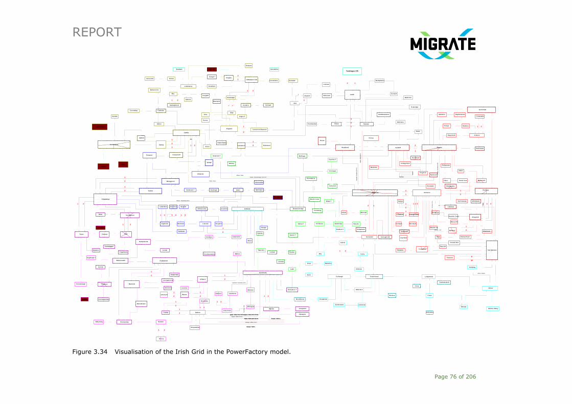
REPORT
Page 76 of 206
Figure 3.34 Visualisation of the Irish Grid in the PowerFactory model.
2
1
2
1
2
1
21
1
2
21
2
1
3
2
1
12
1 2
21
21
2
1
2
1
321
1
2
2
1
1 2
2
1
2
1
21
2
1
2
1
2
1
2
1
2
31
2
1
21
3
2
1
21
21
4321
21
21
21
2
1
2
1
W
E
12
1 2
Caraunduff
Clonee
Coomataggart
Barnadivane
Castletownmoor
Slievecallan
Whitebank
Kilpaddoge
Cordal
BarnakyleCorkagh
Sliabh Bawn
Mulreavy
Clogher
Knockalough
Buffy
Uggool
Knockranny
Fortunesto..
Knockanure
Ballynahulla
Strabane Enniskillen
Tandragee 275
Ballyvouskill
Cloghboola
Woodhouse
Kill Hill
Screebe
Knockacummer
Newbury
Bancroft
Athea
Mount Lucas
Reamore
Cloghran
Crory
Banoge
Glenree
Portan
Cauteen
Nenagh
Killonan
Trabeg
Boggeragh
Tarbert
Castledockrell
Lodgewood
Baroda
Srananagh
Athlone
Tonroe
Kilmore
Kellis
Kilkenny
Dundalk
Knockraha
Raffeen
Clashavoon
Carrowbeg
Shelton Abbey
Arklow
FinglasCorduffWoodland
Gorman
Salthill
Dromada
Glanagow
Kilbarry
Marina
Tynagh
Galway
Cashla
Grange
Wexford
Longpoint
Nangor
Maynooth
Kilmahud
Heuston Sq
Garvagh
Fassaroe
Great Island
Cookstown
Knockumber Navan
Ryebrook
Cullenagh
Pottery Road
Blackrock
Central Park
Taney
North Quays
Milltown
Misery Hill
RingsendHarolds Cross
City West
Francis St
Grange Castle
Griffinrath
Ballywater
Crane
Ballybeg
Irishtown
Mullingar
Thornsberry
Derryiron
Kinnegad
Dunfirth T
Rinawade
Cushaling
Blake T
Kilteel Monread
Newbridge
Stratford T Pollaphuca
Carlow
Dunstown
Dallow T Portlaoise
Athy
Waterford
Killo teranButlerstown
Dungarvan
Ballydine
Anner
Doon
Lisheen Thurles
Barrymore T
Cahir
Ikerrin T
Tipperary
Aghada
Midleton
CastleviewOldcourt
Bandon
Coolroe
Garrow
Glanlee
Whitegate
Cow Cross
Barnahely
Ringaskiddy
Ballylickey
Liberty St
Inniscarra
Brinny
Dunmanway
Mallow
Carr igadrohid
Macroom
Coomagearlahy
Clonkeen
Oughtragh T
Knockearagh
TrienTralee Clahane
Glenlara Charleville
Ahane
Rathkeale
Castlefarm Seal Rock Mungret
MoneteenAughinish SinglandLimerick
DrumlineArdnacrusha Shannonbridge
Derrybrien
Agannygal
Moneypoint
BooltiaghTullabrack T Ennis
Somerset T
RichmondLanesboroCloon
Dalton
Castlebar
Oldstreet
Prospect
Bellacorrick
Tawnaghmore
Moy
Cunghill
Sligo
Gilra
Carr ick-on-Shannon
Arigna T
Meentycat
Binbane
Shankill
Sorne Hill Tril lick
Lisdrum
Golagh T
Letterkenny Drumkeen
CorraclassyCathaleen's Fall
Corderry
Gortawee
Arva
Ratrussan
Meath Hill
Mullagharlin
Platin
Drybridge
Baltrasna
Shellybanks
Poppintree
Stephenstown
Macetown
College Park
Dardistown
Artane
McDermottWolfe ToneCabra
Pelletstown
Cromcastle
Glasmore
Poolbeg
North Wall
Huntstown
Turlough Hill
Carr ickmines
Louth
Flagford
Inchicore
Fra
ncis
St.
- I
nch
icore
11
0 .
.
Poolb
eg -..
Glanagow - Raffeen ..Glanagow - Raffeen ..
Glanagow - Raffeen 2..Glanagow - Raffeen 2..
Glanagow - Raffeen 220 kV ..
Killonan - Kilpaddoge 220 kV..
Cow
Cro
ss - W
hit.
.
Arklow - Ballybe..
Aghada - Raffeen 220 kV S3 Shea..Aghada - Raffeen 220 kV S3 Shea..
Aghada - Raffeen 220 kV ..
Aghada - Raffeen 220 kV S2 Arm..Aghada - Raffeen 220 kV S2 Arm..
Aghada - Raffeen 220 kV S2 She..Aghada - Raffeen 220 kV S2 She..
Mayn
oot
h - W
oodl
and 2
20 k
V S
..
Milltown - Inch..
Inchicore - Iri..
Castleview - Knockraha 110 kV..
Cashla - Ennis ..
Cashla - Shannonbridge 110 kV S2
Athlone - Shann..
Fin
gla
s -
Shelly
banks 2
20..G
orm
an - M
ayno
oth
22..
DIg
SIL
EN
T

REPORT
Page 77 of 206
Figure 3.35 Visualisation of a Transmission Station in the model of the Irish system.
Modelling in PowerFactory
Synchronous Generators
There are 55 synchronous generators represented in detail in the model. This portfolio
encompasses a wide range of machines with different sizes and characteristics. As an example, the
rated apparent power varies from large Combined Cycle Gas Turbines (CCGTs) of 570 MVA to small
hydro plants of 15-20 MVA. Similarly, normalised inertia constants range from 10 s to 1.3 s. The
T2102
ST101 BOOLTIAGH/TULLABRACK
SB1-2
SA1-2
KILPADDOGE #2PROSPECTKILPADDOGE #1
K2K1
T4201 T4202SB2-4SB1-3 SB1-2
DUNSTOWN
SA2-4SA1-3
OLDSTREET
K4SA1-2
K3
Voltage SetpointActual VoltageMWMVArTrafo Tap
MP1MP3 MP2
MP/6.6 kV A1405.84
405.84
405.84
1
3
3
Money
poin
t T4201
500
MV
A
6
Money
poin
t T4201
500
MV
A
Moneypoin
t T
2102 2
50 M
VA
7
Moneypoin
t T
2102 2
50 M
VA
Money
poin
t T4202
500
MV
A
1
Money
poin
t T4202
500
MV
A
400
kV T
4001
Cabl
e..
400
kV T
4001
Cabl
e..
400 k
V T
4002 C
able
Condu
cto..
400 k
V T
4002 C
able
Condu
cto..
400 k
V T
400
3 C
able
..
400 k
V T
400
3 C
able
..
400 k
V T
400
2 C
able
..
400 k
V T
400
2 C
able
..
400 k
V T
400
1 C
able
..
400 k
V T
400
1 C
able
..
400 k
V T
4003 C
able
Condu
cto..
400 k
V T
4003 C
able
Condu
cto..
Moneyp
oin
t S
T101
31.5
MV
A
12
Moneyp
oin
t S
T101
31.5
MV
A
G~
Moneypoint MP3
Money
poin
t 33
0 M
VA
T4003
3
Money
poin
t 33
0 M
VA
T4003
G~
Moneypoint MP2M
oney
poin
t 33
0 M
VA
T4002
3
Money
poin
t 33
0 M
VA
T4002
G~
Moneypoint MP1
Money
poin
t 33
0 M
VA
T4001
1
Money
poin
t 33
0 M
VA
T4001
DIg
SIL
EN
T

REPORT
Page 78 of 206
synchronous generators are represented in PowerFactory using ElmSym elements and TypSym
type library components. The model parameters correspond to the physical characteristics of each
unit as provided by the manufacturers in their technical datasheets.
Table 3.14 Generation and Load Data in Ireland baseline model.
Area Conventional Generation
[MW]
Wind Generation
[MW]
Demand
[MVA]
DUBLIN 2078 0 1815
MID-WEST 2090 168 413
MIDLANDS 472 414 486
NORTH-EAST 0 201 430
NORTH-WEST 264 609 756
SOUTH-EAST 431 144 580
SOUTH-WEST 1516 1210 756
Generic benchmark controllers have been implemented to represent the dynamic behaviour of
turbine governors and Automatic Voltage Regulators (AVR). These models have been tuned to
produce “reasonable” responses, similar to those observed in real-time operation. It should be
noted that the tuning has been based on professional experience, but validation against actual
responses during system disturbances has not been performed. As such, the dynamic response of
these machines must be interpreted as “typical” rather than exact replica of the conventional
generation portfolio installed in Ireland.
The standard IEEEX1 AVR model was used to represent the excitation system for all synchronous
generators. The standard HYGOV model was used to represent the speed governor in all hydro
plants. The standard IEEEG2 model was used to represent the speed governor in all other
conventional plants. Typical parameters for the controllers can be found in Appendix B.2.
Wind Farms
Wind farms were represented with the new generic models developed by Energynautics for the
MIGRATE project [25]. At the time of data freeze, there were 131 wind farms connected in Ireland.
Implementation of the new generic models in such large volume was soon identified to be
inefficient from a computational point of view. Therefore, model aggregation was performed to
reduce the models to a practical volume. Thirty five individual wind farms were finally represented.
Figure 3.36 shows the geographical location of the aggregated wind farms in the model. The
cumulative amount of installed wind capacity on each area is included in Table 3.14. For simplicity,
all wind farms were represented with the Type 3-A dynamic model using the default parameters
provided by Energynautics. However, some settings had to be changed in order to activate the
voltage control functionality, which is a Grid Code requirement for all generators connected at
transmission voltage levels (i.e. 110 kV and above) [57]. The relevant parameter settings for that

REPORT
Page 79 of 206
functionality can be found in Appendix B.2. Wind farms connected to the distribution network were
configured with fixed power factor.
Load
The general load, as forecasted for each transmission station [55], was represented at the low
voltage side of the TSO/DSO interface transformers. This is typically at 38 kV, 20 kV or 10 kV.
Industrial load connected at transmission level was represented in detail with their contracted
Maximum Import Capacity (MIC) behind the grid connected transformer. The ElmLod element and
TypLod type components available in PowerFactory were used. A total of 266 individual loads are
represented in the model.
The loads were represented as the maximum winter peak value (5000 MW) and scaling factors
were used to simulate lower demand scenarios like summer peak (4000 MW) or summer valley
(1750 MW). For dynamic simulations, the voltage and frequency dependency of the load is
captured with a 50% static load and 50% dynamic load assumption. The parameters used in the
simulations can be found in Appendix B.2.
Other Transmission Network Components
All other transmission network elements like lines, cables, transformers, reactors, capacitor banks,
etc, were represented using standard library components from PowerFactory. The lines and cables
were represented using the actual physical characteristics of the conductors and geometry of the
towers/cables. This approach allows accurate computation of mutual coupling between parallel
circuits. Individual sections of non-homogeneous circuits were represented in detail and connected
in series. This resulted in a total of 1076 line elements and 257 cable system elements. All circuits
were represented with Lumped Parameters (PI model). Two and three winding transformers were
represented in detail using the technical datasheet parameters from each unit. A total of 685
transformers are represented in the model.

REPORT
Page 80 of 206
Figure 3.36 Location of aggregated wind farms in the model of the Irish system.

REPORT
Page 81 of 206
4 Study of Power System Stability
4.1 Introduction
The overall approach used to conduct the study of each stability issue listed in Table 1.2 in
Chapter 1 is schematically illustrated in Figure 4.1. The generic test cases, the reduced size
representation of the GB system and the detailed representation of the Irish system, which were
introduced in Chapter 3, constitute the main inputs to the platform that is used for modelling and
simulation. The modelling, simulation, and scripting functionalities of DIgSILENT PowerFactory are
used in the study and assessment of the frequency performance in the frequency containment
period, large-disturbance rotor angle stability, and small-disturbance voltage stability. PSCAD is the
preferred tool for the study and assessment of sub-synchronous controller interactions. A selected
set of operating conditions (e.g. profile of load and generation dispatch that entails a highly loaded
system) and disturbances of interest (e.g. outage of the biggest power plant), i.e. the worst case
(when the system is prone to instability), is defined in the corresponding platform to ascertain the
consequences of increasing penetration levels of PE-interfaced wind power generation. This
information can be defined by each operator or planner based on the operational experience and is
system dependent.
ModellingSystem layout, component parameters
Selected operating conditions and disturbances
SimulationStability indicatorTime response of system variables
DIgSILENT PowerFactory (RMS simulations)PSCAD (EMT simulations)
Figure 4.1 Approach for the study of power system stability.
For each stability phenomenon, the most widely used indicator (in academia and industry) is
evaluated by using the generic test cases. The GB system is used to further evaluate the indicators
concerning frequency performance in the frequency containment period, large-disturbance rotor
angle stability, and small-disturbance voltage stability. Additional tests concerning frequency
performance in the frequency containment period and large-disturbance rotor angle stability are
done by using the Irish system. Basically, the suitability (to capture the resulting stability degree)
of the indicator is investigated before integrating it into the notion of Key Performance Indicator
(KPI), which is introduced subsequently. Other tools like Python, Matlab, and Microsoft Excel are
used to automate the execution of simulations, data processing, and calculation of indicators from
the time response of selected system variables (e.g. kinetic energy of the system). The rationale
behind the selection of the system variables is addressed as well.
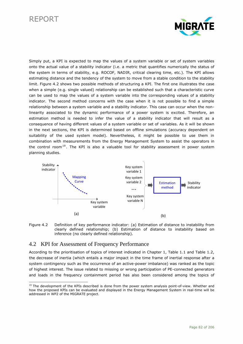
REPORT
Page 82 of 206
Simply put, a KPI is expected to map the values of a system variable or set of system variables
onto the actual value of a stability indicator (i.e. a metric that quantifies numerically the status of
the system in terms of stability, e.g. ROCOF, NADIR, critical clearing time, etc.). The KPI allows
estimating distance and the tendency of the system to move from a stable condition to the stability
limit. Figure 4.2 shows two possible methods of structuring a KPI. The first one illustrates the case
when a simple (e.g. single valued) relationship can be established such that a characteristic curve
can be used to map the values of a system variable into the corresponding values of a stability
indicator. The second method concerns with the case when it is not possible to find a simple
relationship between a system variable and a stability indicator. This case can occur when the non-
linearity associated to the dynamic performance of a power system is excited. Therefore, an
estimation method is needed to infer the value of a stability indicator that will result as a
consequence of having different values of a system variable or set of variables. As it will be shown
in the next sections, the KPI is determined based on offline simulations (accuracy dependent on
suitability of the used system model). Nevertheless, it might be possible to use them in
combination with measurements from the Energy Management System to assist the operators in
the control room19 . The KPI is also a valuable tool for stability assessment in power system
planning studies.
Key system variable
Stability indicator
Mapping Curve
(a)
Key system variable 1
Key system variable 2
Key system variable N
...Estimation
methodStability indicator
(b)
Figure 4.2 Definition of key performance indicator: (a) Estimation of distance to instability from clearly defined relationship; (b) Estimation of distance to instability based on inference (no clearly defined relationship).
4.2 KPI for Assessment of Frequency Performance
According to the prioritisation of topics of interest indicated in Chapter 1, Table 1.1 and Table 1.2,
the decrease of inertia (which entails a major impact in the time frame of inertial response after a
system contingency such as the occurrence of an active-power imbalance) was ranked as the topic
of highest interest. The issue related to missing or wrong participation of PE-connected generators
and loads in the frequency containment period has also been considered among the topics of
19 The development of the KPIs described is done from the power system analysis point-of-view. Whether and how the proposed KPIs can be evaluated and displayed in the Energy Management System in real-time will be addressed in WP2 of the MIGRATE project.

REPORT
Page 83 of 206
highest interest. Therefore, the research outcomes presented in this chapter are related to the time
frame concerning the containment period. The frequency performance in other time frames (e.g.
frequency restoration period) is out of the scope of D1.2.
4.2.1 Frequency Performance in Containment Period
In this section, ROCOF and NADIR are the indicators evaluated to obtain insight about their
suitability with respect to their application in the study of systems with high penetration of
PE-interfaced generation. ROCOF and NADIR are the most widely used indicators by TSOs
worldwide to assess the frequency performance in the frequency containment period [58], [59].
Rate Of Change Of Frequency
The Rate of Change of Frequency (ROCOF) constitutes the frequency gradient after an imbalance
event of active power generation and load demand [60]. The frequency starts to deviate from the
rated value as an immediate result of a generation loss. Figure 4.3 illustrates the variation of the
frequency, as an example, for the variation of the frequency for different values of inertia in
generic test case 1.
Figure 4.3 Illustration of different slopes for different values of inertia.
The ROCOF, which results during the first instants after the time of occurrence of an event (e.g.
generator outage) that causes imbalance in a power system, is defined as follows [39]:
where f stands for frequency (in Hz).
ROCOF =𝑑𝑓
𝑑𝑡 (4.1)
NADIR

REPORT
Page 84 of 206
For a synchronous generator, the first time derivative of the frequency, 𝑑𝑓
𝑑𝑡 , can be determined from
the per-unit formulation of its swing equation [12], that is:
where:
∆𝑃 = the change of the active power (e.g. amount of MW lost due to a generator outage)
f0 = the nominal frequency (Hz)
H𝑖 = the inertia constant of the generator (s)
TN−𝑖 = the acceleration time constant (s)
(i.e. time in seconds it takes to accelerate a generator from standstill to nominal speed)
SB−𝑖 = the nominal apparent power of the generator (MVA) [61]
i = the i-th generator among n generators in the system
The relationship between the kinetic energy stored in the rotating masses (MWs), Ekin−𝑖 , at
nominal speed and the inertia constant H𝑖 of a synchronous generator is defined by [62], [63].
The total kinetic energy of the system is computed by [63]:
where n is the number of synchronous generators in the system.
Equation (4.5) is determined by substituting equation (4.3) into (4.2). It can be seen that the
ROCOF is inversely proportional to the kinetic energy (as it does with the inertia constant in
equation (4.2)).
Motivated by equation (4.5), an approximation of ROCOF, as shown in equation (4.6) is suggested
in [64] and [65] for qualitative assessment of the frequency performance within the time window
of the system inertial response.
𝑑𝑓
𝑑𝑡=
∆PSB−𝑖2H𝑖
f0 =
∆PSB−𝑖TN−𝑖
f0 (4.2)
Ekin−𝑖 = H𝑖 ∙ SB−𝑖 (4.3)
Ekin−sys = ∑ Ekin−𝑖𝑛
𝑖=1 (4.4)
𝑑𝑓
𝑑𝑡=
∆P
2 ∙ Ekin−𝑖f0 (4.5)
ROCOF =∆Psys
2(Ekin−sys − Ekin−lost)f0 (4.6)
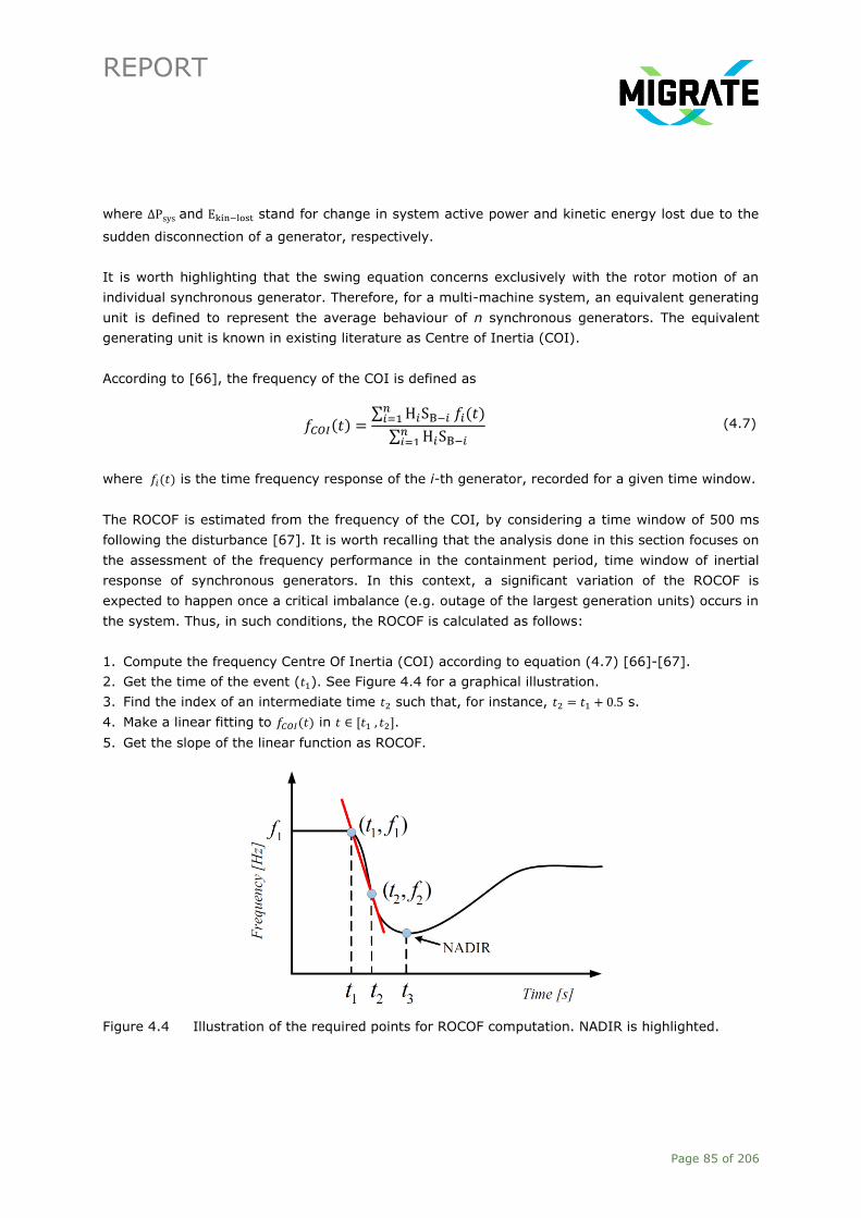
REPORT
Page 85 of 206
where ∆Psys and Ekin−lost stand for change in system active power and kinetic energy lost due to the
sudden disconnection of a generator, respectively.
It is worth highlighting that the swing equation concerns exclusively with the rotor motion of an
individual synchronous generator. Therefore, for a multi-machine system, an equivalent generating
unit is defined to represent the average behaviour of n synchronous generators. The equivalent
generating unit is known in existing literature as Centre of Inertia (COI).
According to [66], the frequency of the COI is defined as
where 𝑓𝑖(𝑡) is the time frequency response of the i-th generator, recorded for a given time window.
The ROCOF is estimated from the frequency of the COI, by considering a time window of 500 ms
following the disturbance [67]. It is worth recalling that the analysis done in this section focuses on
the assessment of the frequency performance in the containment period, time window of inertial
response of synchronous generators. In this context, a significant variation of the ROCOF is
expected to happen once a critical imbalance (e.g. outage of the largest generation units) occurs in
the system. Thus, in such conditions, the ROCOF is calculated as follows:
1. Compute the frequency Centre Of Inertia (COI) according to equation (4.7) [66]-[67].
2. Get the time of the event (𝑡1). See Figure 4.4 for a graphical illustration.
3. Find the index of an intermediate time 𝑡2 such that, for instance, 𝑡2 = 𝑡1 + 0.5 s.
4. Make a linear fitting to 𝑓𝐶𝑂𝐼(𝑡) in 𝑡 ∈ [𝑡1 , 𝑡2].
5. Get the slope of the linear function as ROCOF.
Figure 4.4 Illustration of the required points for ROCOF computation. NADIR is highlighted.
𝑓𝐶𝑂𝐼(𝑡) =∑ H𝑖SB−𝑖 𝑓𝑖(𝑡)𝑛𝑖=1
∑ H𝑖SB−𝑖𝑛𝑖=1
(4.7)

REPORT
Page 86 of 206
The normative contingencies for the interconnected operation in Continental Europe, as defined by
ENTSO-E in [39] and [59] for the ROCOF computation is the tripping of the two largest generation
units connected to the same busbar. The maximum value of ROCOF allowed in the Great Britain
system is 125 mHz/s, whereas for continental Europe values between 500 mHz/s and 1 Hz/s have
been recorded [59].
It should be mentioned that in this study, the frequency of the COI in the system under study is
used for the calculation of ROCOF. Although being out of scope of D1.2, because the focus is on a
systemic issue, it is worth pointing out that in case of having a system with several regions with
different inertia characteristics, the same methodology based on frequency of the COI can be
applied for each of the regions.
NADIR
This indicator corresponds to the lower frequency value obtained after a power imbalance which
depends on the system inertia, the response of the available frequency containment reserves, the
size and location of the disturbance, and the pre-disturbance operating conditions. In Figure 4.3,
this value is highlighted with a dot of the corresponding colour for each curve, and is pointed out in
Figure 4.4 as well [68].
The criterion that defines the limit for NADIR is expressed as
𝑓𝑁𝑎𝑑𝑖𝑟 ≥ 𝑓𝑚𝑖𝑛 (4.8)
where fmin is the minimum acceptable frequency defined in the grid code.
This indicator has a high relevance in the frequency control procedures because a low value (lower
than 47.5 Hz) might violate the security thresholds and a blackout can hardly be avoided [39] due
to the disconnection of generation units at this frequency. However, in order to avoid load shedding,
the maximum frequency deviation is defined as -800 mHz in continental Europe as stated in
sections A-D2.3 and A-D2.4 of [59], which represents a NADIR of 49.2 Hz.
4.2.2 Analysis of ROCOF and NADIR using Generic Test Case 1
Automating Data Extraction and Processing
The power system dynamics is simulated by using DIgSILENT PowerFactory. This software allows
an interaction with Python which can be exploited to automate the execution of simulation and data
extraction. Thus, the Python-PowerFactory interface is used to call the set of defined dispatch
scenarios (cf. Figure 3.16 in Chapter 3) from an external file (Excel data base). Matlab scripts are
used to process the data obtained from the simulations in PowerFactory and calculate the ROCOF
and NADIR. The overall procedure is schematically shown in Figure 4.5. Please note that the user
has the option to customise the process to automatically define different system topologies.

REPORT
Page 87 of 206
Start
Run RMS simulation time_DB
All Dispatch
cases?
i++
Finish
Load dispatch cases
i=1
Select dispatch case(i)
Dispatch cases
...
Load Case1
Ld1
Ld2
...
D1
D2
Ldn Dn
... CaseM
... ...
D1
D2
Dn
...
......
Gen Case1
G01
G02
...
D1
D2
Gn Dn
... CaseM
... ...
D1
D2
Dn
...
...
...
Yes
Branch
outage?
No
Set line out of
service
No
Yes
SS_DB
Set event
Automated
simulation and data
extraction
Data Processing
Run load flow
Figure 4.5 Procedure for automated simulation and data extraction by combining PowerFactory, Python, Matlab, and Excel. SS_DB stands for database of initial conditions (steady-state), whereas time_DB stands for database of time responses of system variables.
An example of dispatch scenarios is shown in Table 4.1, where the synchronous generators’
dispatch for winter season is shown. The character X indicates that a synchronous generator is out
of service. This table represents several situations, where the synchronous generation dispatch
changes due to the shift from low to high share from wind generation. It is worth clarifying that
synchronous generators in Area A belong to hydro power plants (another type of renewable energy
based power plant) and are kept as base plants in all operational scenarios. Besides, it is
highlighted that the diversity of dispatches shown in Table 4.1 entail different levels of inertia (also
different levels of kinetic energy) and different geographical spread of power electronic interfaced
wind generation within Area B as well as within Area C. The load information is selected according

REPORT
Page 88 of 206
to the seasons presented in Chapter 3, Section 3.2.3, for generic test case1 (Winter, Spring or
Summer) as 100%, 80% or 60% of Winter peak load. The procedure of creating different
operational scenarios illustrated in Figure 3.16.
Table 4.1 Synchronous generator dispatch for Winter season (in MW).
Operational scenario
Sync Gen 1 2 3 4 5 6 7 8 9 10
A1aG 1000 1000 1000 1000 1000 1000 1000 1000 1000 1000
A1bG 1000 1000 1000 1000 1000 1000 1000 1000 1000 1000
A2aG 1000 1000 1000 1000 1000 1000 1000 1000 1000 1000
A2bG 1000 1000 1000 1000 1000 1000 1000 1000 1000 1000
A3G 400 400 400 400 400 400 400 400 400 400
A6G 440 440 440 440 440 440 440 440 440 440
B10G 950 X X X X X X X X X
B2aG 1200 1200 X X X X X X X X
B2bG 1200 1200 1200 X X X X X X X
B3G 1401.7 1401.7 1401.7 1401.7 X X X X X X
B8G 900 900 900 900 900 X X X X X
C10G 850 850 850 850 850 850 X X X X
C12G 1150 1150 1150 1150 1150 1150 1150 X X X
C14G 850 850 850 850 850 850 850 850 X X
C2G 1300.0 1300.0 1300.0 1300.0 1300.0 1300.0 1300.0 1300.0 1300.0 X
C7G 1300.0 1300.0 1300.0 1300.0 1300.0 1300.0 1300.0 1300.0 1300.0 1300.0
Total generation (Synchronous) 15941.7 14991.7 13791.7 12591.7 11190 10290 9440 8290 7440 6140
Total losses 215.5 216.05 220.21 224.37 229.12 229.17 229.23 228.94 228.95 232.93
Total Load 15565 15565 15565 15565 15565 15565 15565 15565 15565 15565
To illustrate the effects of increasing of wind penetration, the following three cases for Winter
(Case 1, Case 5 and Case10 according the dispatches in Table 4.1) are analysed. In Case 1, the
whole system is fully supplied by conventional power plants with synchronous generators. In
Case 5, Areas A and C remain with all plants with synchronous generators in operation, whereas
Area B has only one plant with synchronous generators in operation and the other plants are
replaced by wind power plants. In Case10, Area A still remains with all plants with synchronous
generators in operation, Area B has 100 % of penetration of wind generation, and Area C has only
one plant with synchronous generators in operation and the other plants are replaced by wind
power plants. In all cases the imbalance is caused by the sudden outage of the conventional power
plant A1bG in Area A (which represents 6.3% of total generation).
As shown in Figure 4.6 (Case 1), since all the areas are based on synchronous generation, the
frequency of the COI and the values of system indicators (ROCOF/NADIR) are affected by all three

REPORT
Page 89 of 206
areas. Note also that inter-area low frequency oscillations involving the three areas are highly
excited by the occurrence of the imbalance.
Figure 4.6 Frequency responses, Case 1: Conventional power plants with synchronous generation in all areas.
Figure 4.7 Frequency responses, Case 5: Areas A and C with all conventional plants in operation, Area B with only one conventional plant in operation.
In Figure 4.7 (Case 5), as it happens in Figure 4.6, the synchronous generators in Area A
experience a higher frequency gradient, since they are located in the Area in which the imbalance
occurs. A similar observation was reported in [65]. Additionally, note in Figure 4.7 that the
frequency of the COI is mainly affected by Areas A and C, and it can also be seen that the
remaining synchronous generation in Area B follows the average (i.e. experiences less frequency
gradient than generators in Area A). In this case, the inter-area low frequency oscillations are less
excited, whereas ROCOF and NADIR worsen significantly.

REPORT
Page 90 of 206
Figure 4.8 Frequency responses, Case 10: Area A with all conventional plants in operation, Area B with 100% penetration of wind generation, Area C with only one conventional plant in operation.
Lastly, note in Figure 4.8 (Case 10) that all remaining synchronous generators follow very closely
the COI, whereas the inter-area oscillations are not excited, the ROCOF and NADIR worsen even
more w.r.t Case 5, and the frequency performance deteriorates dramatically after the NADIR. For
sake of illustration, the measured frequency in Case 10 for one bus of Area B (which has no
synchronous generators) is shown in Figure 4.9. This corresponds with the measured frequency of
the voltage in node 21 (the common coupling node of wind park 10B, cf. Figure 3.15). It can be
seen that the frequency response in Area B follows very closely the frequency of the COI.
Figure 4.9 Frequency of the voltage at node 21, Case 10: Area B with 100% penetration of wind generation.

REPORT
Page 91 of 206
The remainder of this section focuses on three aspects:
1. Analysis of ROCOF and NADIR by using generic test case 1 (cf. Section 3.2.3). The ROCOF and
NADIR resulting from different levels of kinetic energy of the system (due to different levels of
inertia as a consequence of different wind penetration levels) and the effects of different load
model parameters on ROCOF and NADIR are investigated.
2. Further investigation on the findings from generic test case 1 by using an academic (reduced
size) model of the GB system (cf. Section 3.3.2) provided by the University of Manchester and
proposition of a methodology for KPI for frequency performance in the frequency containment
period
3. Additional tests based on the Irish system (cf. Section 3.3.3).
Calculation of ROCOF and Frequency NADIR
The computational procedure to determine the ROCOF and NADIR for the simulations run in this
work is shown in Figure 4.10. Once the data base with the generators frequency response is
obtained (time_ DB block in Figure 4.10) in the data extraction step (cf. Figure 4.5), the raw data
is migrated to MATLAB to begin the processing. The structure of the data base is such that there
exists one csv-file per each simulation case, for which the entire set of simulations needs to be
examined. Each csv-file has the time series and the corresponding frequency values associated to
the dynamic response of each active (i.e. in service) synchronous generator in the system.
Therefore, this information is used to compute the fCOI(t), from which the ROCOF is obtained.
As mentioned in Section 4.2.1, the common practice is to compute the frequency of the Centre-Of-
Inertia (COI), which constitutes an equivalent representation of the frequency response of the
entire system. In other words, each system can be seen as a single generator with an equivalent
inertia and its representative centroid frequency.
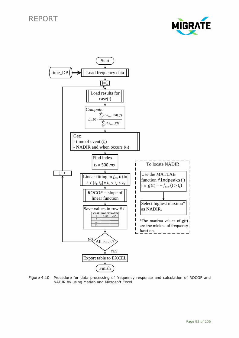
REPORT
Page 92 of 206
Start
time_DB Load frequency data
i=1
Load results for
case(i)
Compute:
,
1
,
1
( )
( )
n
i base i i
iCOI n
i base i
i
H S PMf t
f t
H S PM
Get:
- time of event ( )
- NADIR and when occurs ( )1t
Find index:
Linear fitting to in ( )COIf t
ROCOF = slope of
linear function
Save values in row # iCASE ROCOF
1
2
...
0.119
M
NADIR
49.5
All cases?
i++
Export table to EXCEL
Finish
NO
YES
To locate NADIR
Use the MATLAB
function findpeaks()
in: 1( ) ( )COIg t f t t
Select highest maxima*
as NADIR.
*The maxima values of g(t) are the minima of frequency function.
t3
t2 = 500 ms
Figure 4.10 Procedure for data processing of frequency response and calculation of ROCOF and NADIR by using Matlab and Microsoft Excel.

REPORT
Page 93 of 206
Figure 4.11 shows the frequency response of all generators in the generic test case 1 when a
generator unit that entails 10% of total generated active power gets suddenly out of service. The
event occurs at t=26 s.
Figure 4.11 Synchronous generators’ frequency response to an imbalance caused by 10%
generation loss, the frequency associated to the COI is shown by the red dotted line.
In the investigations done with all systems considered in this deliverable, the time window where
the slope of the frequency is computed is fixed to 0.5 s after the occurrence of the disturbance. As
shown in Figure 4.4, the window defined by [t1, t2] is the period of interest for ROCOF computation.
A linear fitting on in this time window will represent a suitable approximation of the actual rate of
change of frequency as can be seen in Figure 4.12.
Figure 4.12 Frequency of the COI. The time window for ROCOF computation is highlighted in red.
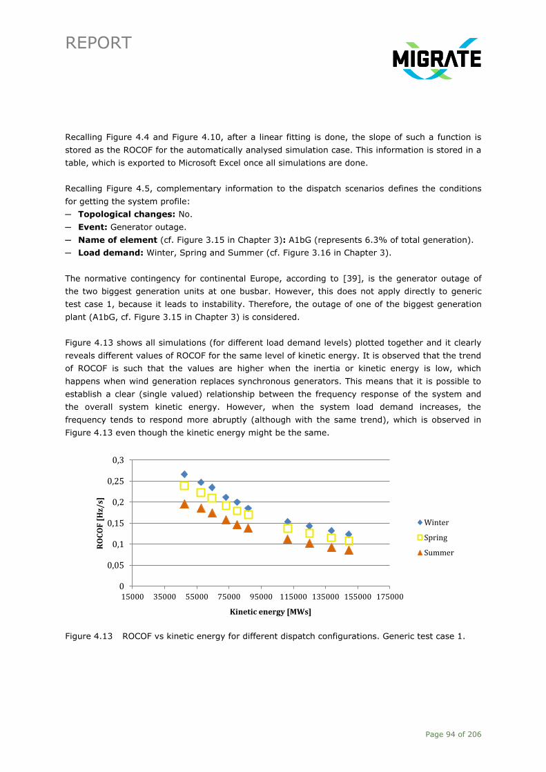
REPORT
Page 94 of 206
Recalling Figure 4.4 and Figure 4.10, after a linear fitting is done, the slope of such a function is
stored as the ROCOF for the automatically analysed simulation case. This information is stored in a
table, which is exported to Microsoft Excel once all simulations are done.
Recalling Figure 4.5, complementary information to the dispatch scenarios defines the conditions
for getting the system profile:
─ Topological changes: No.
─ Event: Generator outage.
─ Name of element (cf. Figure 3.15 in Chapter 3): A1bG (represents 6.3% of total generation).
─ Load demand: Winter, Spring and Summer (cf. Figure 3.16 in Chapter 3).
The normative contingency for continental Europe, according to [39], is the generator outage of
the two biggest generation units at one busbar. However, this does not apply directly to generic
test case 1, because it leads to instability. Therefore, the outage of one of the biggest generation
plant (A1bG, cf. Figure 3.15 in Chapter 3) is considered.
Figure 4.13 shows all simulations (for different load demand levels) plotted together and it clearly
reveals different values of ROCOF for the same level of kinetic energy. It is observed that the trend
of ROCOF is such that the values are higher when the inertia or kinetic energy is low, which
happens when wind generation replaces synchronous generators. This means that it is possible to
establish a clear (single valued) relationship between the frequency response of the system and
the overall system kinetic energy. However, when the system load demand increases, the
frequency tends to respond more abruptly (although with the same trend), which is observed in
Figure 4.13 even though the kinetic energy might be the same.
Figure 4.13 ROCOF vs kinetic energy for different dispatch configurations. Generic test case 1.
0
0,05
0,1
0,15
0,2
0,25
0,3
15000 35000 55000 75000 95000 115000 135000 155000 175000
RO
CO
F [
Hz/
s]
Kinetic energy [MWs]
Winter
Spring
Summer
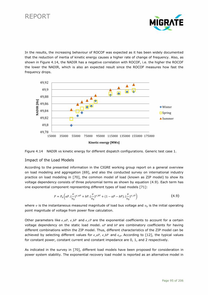
REPORT
Page 95 of 206
In the results, the increasing behaviour of ROCOF was expected as it has been widely documented
that the reduction of inertia of kinetic energy causes a higher rate of change of frequency. Also, as
shown in Figure 4.14, the NADIR has a negative correlation with ROCOF, i.e. the higher the ROCOF
the lower the NADIR, which is also an expected result since the ROCOF measures how fast the
frequency drops.
Figure 4.14 NADIR vs kinetic energy for different dispatch configurations. Generic test case 1.
Impact of the Load Models
According to the presented information in the CIGRE working group report on a general overview
on load modeling and aggregation [69], and also the conducted survey on international industry
practice on load modeling in [70], the common model of load (known as ZIP model) to show its
voltage dependency consists of three polynomial terms as shown by equation (4.9). Each term has
one exponential component representing different types of load models [71]:
𝑃 = 𝑃0 (𝑎𝑃. (𝑣
𝑣0)𝑒_𝑎𝑃 + 𝑏𝑃. (
𝑣
𝑣0)𝑒_𝑏𝑃 + (1 − 𝑎𝑃 − 𝑏𝑃). (
𝑣
𝑣0)𝑒_𝑐𝑃) (4.9)
where 𝑣 is the instantaneous measured magnitude of load bus voltage and 𝑣0 is the initial operating
point magnitude of voltage from power flow calculation.
Other parameters like 𝑒_𝑎𝑃, 𝑒_𝑏𝑃 and 𝑒_𝑐𝑃 are the exponential coefficients to account for a certain
voltage dependency on the static load model. 𝑎𝑃 and 𝑏𝑃 are combinatory coefficients for having
different combinations within the ZIP model. Thus, different characteristics of the ZIP model can be
achieved by selecting different values for 𝑒_𝑎𝑃, 𝑒_𝑏𝑃 and 𝑒𝑐𝑃 . According to [12], the typical values
for constant power, constant current and constant impedance are 0, 1, and 2 respectively.
As indicated in the survey in [70], different load models have been proposed for consideration in
power system stability. The exponential recovery load model is reported as an alternative model in
49,78
49,8
49,82
49,84
49,86
49,88
49,9
49,92
15000 35000 55000 75000 95000 115000 135000 155000 175000
NA
DIR
[H
z]
Kinetic energy [MWs]
Winter
Spring
Summer
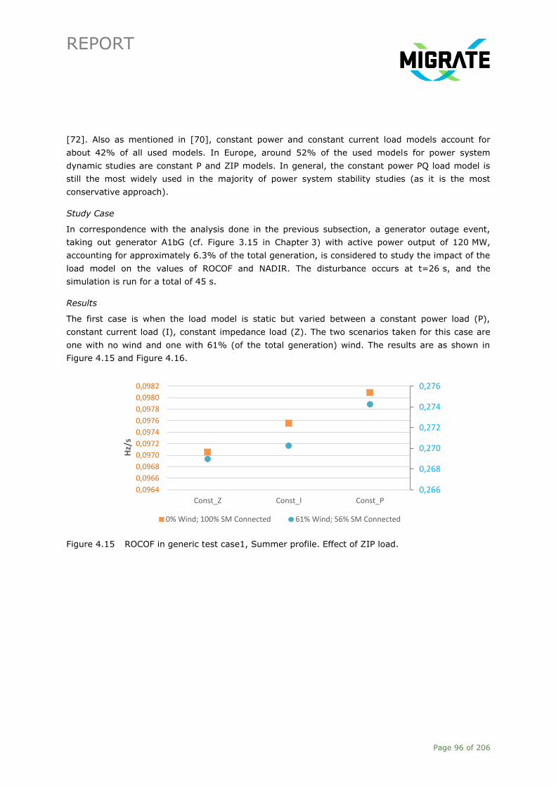
REPORT
Page 96 of 206
[72]. Also as mentioned in [70], constant power and constant current load models account for
about 42% of all used models. In Europe, around 52% of the used models for power system
dynamic studies are constant P and ZIP models. In general, the constant power PQ load model is
still the most widely used in the majority of power system stability studies (as it is the most
conservative approach).
Study Case
In correspondence with the analysis done in the previous subsection, a generator outage event,
taking out generator A1bG (cf. Figure 3.15 in Chapter 3) with active power output of 120 MW,
accounting for approximately 6.3% of the total generation, is considered to study the impact of the
load model on the values of ROCOF and NADIR. The disturbance occurs at t=26 s, and the
simulation is run for a total of 45 s.
Results
The first case is when the load model is static but varied between a constant power load (P),
constant current load (I), constant impedance load (Z). The two scenarios taken for this case are
one with no wind and one with 61% (of the total generation) wind. The results are as shown in
Figure 4.15 and Figure 4.16.
Figure 4.15 ROCOF in generic test case1, Summer profile. Effect of ZIP load.
0,266
0,268
0,270
0,272
0,274
0,276
0,0964
0,0966
0,0968
0,0970
0,0972
0,0974
0,0976
0,0978
0,0980
0,0982
Const_Z Const_I Const_P
Hz/
s
0% Wind; 100% SM Connected 61% Wind; 56% SM Connected

REPORT
Page 97 of 206
Figure 4.16 NADIR in generic test case1, Summer profile. Effect of ZIP load.
It can be seen from these graphs that different load models give some insights into the importance
of load modelling. For both the high and the low wind scenario, it can be seen that the worst
results are obtained for constant power loads. This is because the power requirement of the load
remains constant despite the network conditions, unlike constant current (linear voltage
relationship) and constant impedance (quadratic voltage relationship). This means that for constant
power load scenarios, the current increases, which causes more strain on network and hence,
worse system indicators [53]. Under non-constant voltage relationship (as in constant I and
constant Z loads), the voltage drop in the system reduces the amount of power required by the
such loads in the system. Which means, after occurrence of the disturbance, the voltage profile will
be affected in some buses and due to the voltage dependency of loads, the loads are adjusted as
well. Power electronics-interfaced loads, when well regulated, behave as constant power loads [73].
As more and more loads are being PE-interfaced in form of motor drives, ac-dc converters, the
worst case scenario can be effectively represented by constant power load models. This is
supported by the analysis in Section 4.2.3 as well. A similar effect can be seen in the winter
scenarios where the system is more highly loaded. Figure 4.17 and Figure 4.18 below corroborate
this fact.
49,775
49,780
49,785
49,790
49,795
49,800
49,900
49,902
49,904
49,906
49,908
49,910
49,912
49,914
Const_Z Const_I Const_P
Hz
0% Wind; 100% SM Connected 61% Wind; 56% SM Connected
0,2530
0,2532
0,2534
0,2536
0,2538
0,2540
0,2542
0,1466
0,1468
0,1470
0,1472
0,1474
0,1476
0,1478
0,1480
Const_Z Const_I Const_P
Hz/
s
Low Wind High Wind
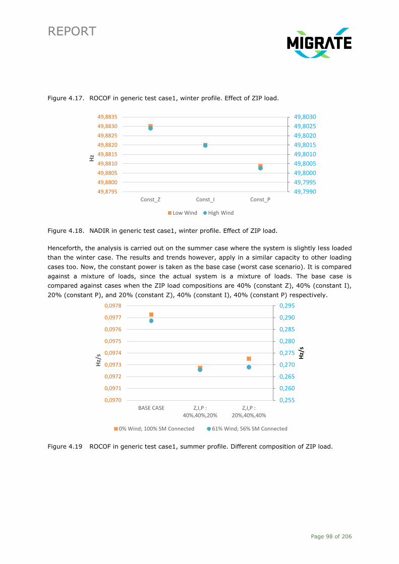
REPORT
Page 98 of 206
Figure 4.17. ROCOF in generic test case1, winter profile. Effect of ZIP load.
Figure 4.18. NADIR in generic test case1, winter profile. Effect of ZIP load.
Henceforth, the analysis is carried out on the summer case where the system is slightly less loaded
than the winter case. The results and trends however, apply in a similar capacity to other loading
cases too. Now, the constant power is taken as the base case (worst case scenario). It is compared
against a mixture of loads, since the actual system is a mixture of loads. The base case is
compared against cases when the ZIP load compositions are 40% (constant Z), 40% (constant I),
20% (constant P), and 20% (constant Z), 40% (constant I), 40% (constant P) respectively.
Figure 4.19 ROCOF in generic test case1, summer profile. Different composition of ZIP load.
49,7990
49,7995
49,8000
49,8005
49,8010
49,8015
49,8020
49,8025
49,8030
49,8795
49,8800
49,8805
49,8810
49,8815
49,8820
49,8825
49,8830
49,8835
Const_Z Const_I Const_P
Hz
Low Wind High Wind
0,255
0,260
0,265
0,270
0,275
0,280
0,285
0,290
0,295
0,0970
0,0971
0,0972
0,0973
0,0974
0,0975
0,0976
0,0977
0,0978
BASE CASE Z,I,P :40%,40%,20%
Z,I,P :20%,40%,40%
Hz/
s
Hz/
s
0% Wind; 100% SM Connected 61% Wind; 56% SM Connected

REPORT
Page 99 of 206
Figure 4.20 NADIR in generic test case1, summer profile. Different composition of ZIP load.
From Figure 4.19 and Figure 4.20, as expected, the mixture of loads is better than in the base case.
However, as the percentage of constant power load is increased, the ROCOF and NADIR indicators
get worse (although the difference between the two additional scenarios is not much). This is
expected since the load moves more towards a constant power characteristic.
For the next case, the ZIP ratio is kept as 20%, 40%, 40% to have a load profile closer to constant
power, but also a mixture of other loads. Next, the inclusion of induction motor loads in the system
is analysed. Most of the load in the power system is industrial load (mostly induction motor load).
The amount of induction motor load in the system is varied in steps of 25% between 0 and 75%.
Figure 4.21 and Figure 4.22 show an interesting characteristic in this case. It is necessary to
differentiate the scales in this case for the two scenarios of high and low wind since the results’
profiles cannot be correctly visualised otherwise. On the left y axis is the scale for the low wind
scenario while on the right is for the scenario of high wind penetration. It is observed that the
system progressively becomes worse when more and more induction motors are added. ROCOF is
increased while the NADIR is decreased. This can be explained by induction motor operating
characteristics themselves. Induction motor operating characteristics are directly related to system
frequency. Any change in system frequency directly reflects on the motor speed. In an induction
motor, the frequency determines the speed (and therefore inertia) unlike the synchronous motor,
where the speed (and therefore inertia) determines the frequency. As already mentioned, it is
essential to analyse the impact of induction motor load since it is dominant. This analyses gives is
good indication of the importance of addition of dynamic load. Note also that the impact of a high
amount of induction motors is more prominent in a system with high penetration of power
electronics-interfaced generation. By contrast, the impact is small in a system dominated by
conventional plants with synchronous generators, which have a better voltage regulation behaviour
49,55
49,60
49,65
49,70
49,75
49,80
49,85
49,84
49,85
49,86
49,87
49,88
49,89
49,90
49,91
49,92
BASE CASE Z,I,P : 40%,40%,20%Z,I,P : 20%,40%,40%
Hz
Hz
0% Wind; 100% SM Connected 61% Wind; 56% SM Connected

REPORT
Page 100 of 206
(w.r.t. voltage regulation capability of power electronics-interfaced generation), and this prevents
high variability of the voltage magnitudes of the buses to which loads are connected.
Figure 4.21 ROCOF in generic test case1, summer profile. Effect of induction motors.
However, recently most of the induction motor loads are being interfaced by PE-based drives.
Hence, it is needed to include the effect of having PE in the system. For this purpose, in the next
analysis the induction motor percentage is set to a conservative 25% and includes PE-based
aggregated load. This load model is a composite load model derived from [53], and can effectively
be used to aggregate distributed generation and PE-interfaced load.
In an initial study, it is attempted to replace the conventional loads in area C of generic test case 1
(i.e. the area with the highest load and least wind generation). For one scenario, 1 conventional
load is replaced with aggregated Distributed Generation and load (DG-load), and for the second
scenario, 3 conventional loads are replaced with aggregated DG-loads. The results are shown in
Figure 4.23 and Figure 4.24. From these figures, the inclusion of Distributed Energy Resources
(DER) seems to have a positive impact on the system’s ROCOF and NADIR. This can be attributed
to the fact that the DER contribute to reduce the system active power loss even in case of
disturbances. This is in strong contrast to earlier cases where DGs were seen as ‘static negative
loads’, disconnected in event of disturbances (e.g. voltage below 0.8 pu). The DER model used in
[53] has a complex control structure that is able to aggregate large amounts of technologically
diverse DGs (non-LVRT, LVRT, aRCI, aRACI supporting) effectively and produce aggregated
behaviour that can reflect the support from DGs to the grid. It is thus recommended that
conventional loads should be replaced with composite load models.
0,315
0,316
0,317
0,318
0,319
0,320
0,321
0,322
0,323
0,1043
0,1044
0,1045
0,1046
0,1047
0,1048
0,1049
0,1050
0,1051
0,1052
0,1053
0,1054
0% 25% 50% 75%
Hz/
s
0% Wind; 100% SM Connected 61% Wind; 56% SM Connected
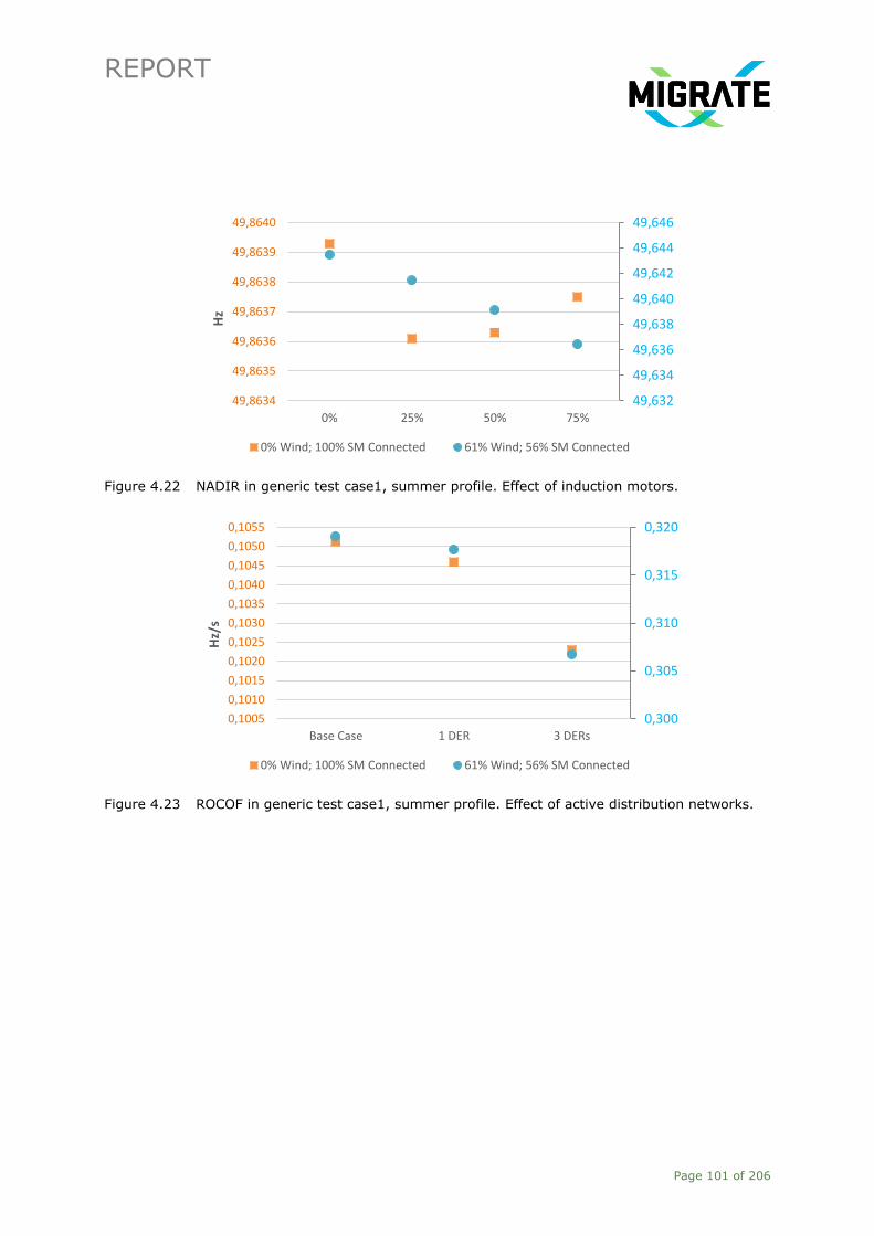
REPORT
Page 101 of 206
Figure 4.22 NADIR in generic test case1, summer profile. Effect of induction motors.
Figure 4.23 ROCOF in generic test case1, summer profile. Effect of active distribution networks.
49,632
49,634
49,636
49,638
49,640
49,642
49,644
49,646
49,8634
49,8635
49,8636
49,8637
49,8638
49,8639
49,8640
0% 25% 50% 75%
Hz
0% Wind; 100% SM Connected 61% Wind; 56% SM Connected
0,300
0,305
0,310
0,315
0,320
0,1005
0,1010
0,1015
0,1020
0,1025
0,1030
0,1035
0,1040
0,1045
0,1050
0,1055
Base Case 1 DER 3 DERs
Hz/
s
0% Wind; 100% SM Connected 61% Wind; 56% SM Connected

REPORT
Page 102 of 206
Figure 4.24 NADIR in generic test case1, summer profile. Effect of active distribution networks.
4.2.3 Proposition of KPI for Assessment of Frequency Performance
Based on the findings with generic test case 1The main stability indicators used for the proposed
frequency KPI in this study are ROCOF and NADIR. Because, as shown with generic test case 1,
these indicators are still suitable for assessment with high penetration levels of wind power and
also considering the impact of load modelling. As indicated in Section 4.1, the proposed KPI is
expected to map the values of system variables onto the actual value of a stability indicator
(ROCOF/NADIR). Here, the key system variable is the system kinetic energy, whereas load power
deviations and losses deviations are studied in this section to ascertain their influence. It should be
noted that, inertia can be used as an alternative, provided that a reliable estimate is available to
ensure enough confidence in the monitoring task in the control room. According to the fundamental
physics of the motion, system inertia can be derived according to the moment of inertia of all
rotating masses synchronously rotating in the system which will result in system kinetic energy.
As a result of previous analysis with generic test case 1, it is important to point out that it is
necessary to ascertain other system variables (in addition to the level of kinetic energy of the
system) which can give more insight on the frequency behaviour in the frequency containment
period (changes in ROCOF and NADIR). For sake of further analysis, recalling equation (4.2),
ROCOF and kinetic energy have an inverse relationship, i.e. lower kinetic energy leads to a higher
value of ROCOF. This relationship can be considered as the main factor in frequency performance
assessment in the frequency containment period. But in order to get more insight about the fact of
having different values of ROCOF for the same level of kinetic energy and in different loading levels
with different generation dispatch and COI (cf. Figure 4.13), analysis of additional variables mainly
from the grid side parameters might be beneficial. These additional variables can be related to
those elements which can affect the variation of power mismatch (∆𝑃 in equation (4.2)).
49,58
49,60
49,62
49,64
49,66
49,68
49,70
49,72
49,74
49,76
49,84
49,85
49,86
49,87
49,88
49,89
49,90
49,91
Base Case 1 DER 3 DERs
Hz
0% Wind; 100% SM Connected 61% Wind; 56% SM Connected
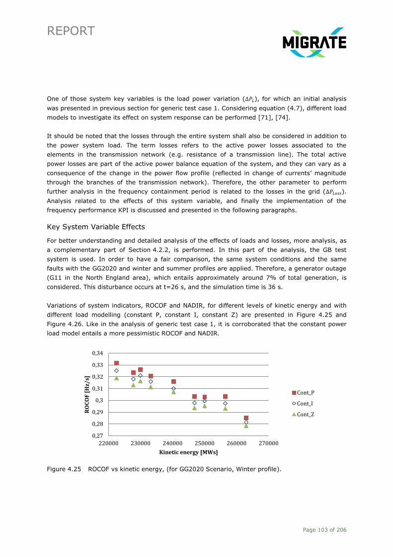
REPORT
Page 103 of 206
One of those system key variables is the load power variation (∆𝑃𝐿), for which an initial analysis
was presented in previous section for generic test case 1. Considering equation (4.7), different load
models to investigate its effect on system response can be performed [71], [74].
It should be noted that the losses through the entire system shall also be considered in addition to
the power system load. The term losses refers to the active power losses associated to the
elements in the transmission network (e.g. resistance of a transmission line). The total active
power losses are part of the active power balance equation of the system, and they can vary as a
consequence of the change in the power flow profile (reflected in change of currents’ magnitude
through the branches of the transmission network). Therefore, the other parameter to perform
further analysis in the frequency containment period is related to the losses in the grid (∆𝑃𝐿𝑜𝑠𝑠).
Analysis related to the effects of this system variable, and finally the implementation of the
frequency performance KPI is discussed and presented in the following paragraphs.
Key System Variable Effects
For better understanding and detailed analysis of the effects of loads and losses, more analysis, as
a complementary part of Section 4.2.2, is performed. In this part of the analysis, the GB test
system is used. In order to have a fair comparison, the same system conditions and the same
faults with the GG2020 and winter and summer profiles are applied. Therefore, a generator outage
(G11 in the North England area), which entails approximately around 7% of total generation, is
considered. This disturbance occurs at t=26 s, and the simulation time is 36 s.
Variations of system indicators, ROCOF and NADIR, for different levels of kinetic energy and with
different load modelling (constant P, constant I, constant Z) are presented in Figure 4.25 and
Figure 4.26. Like in the analysis of generic test case 1, it is corroborated that the constant power
load model entails a more pessimistic ROCOF and NADIR.
Figure 4.25 ROCOF vs kinetic energy, (for GG2020 Scenario, Winter profile).
0,27
0,28
0,29
0,3
0,31
0,32
0,33
0,34
220000 230000 240000 250000 260000 270000
RO
CO
F [
Hz/
s]
Kinetic energy [MWs]
Cont_P
Cont_I
Cont_Z
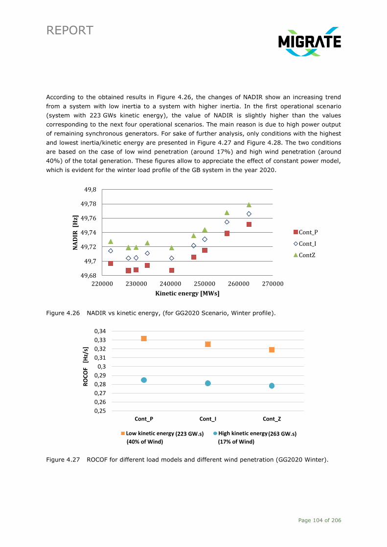
REPORT
Page 104 of 206
According to the obtained results in Figure 4.26, the changes of NADIR show an increasing trend
from a system with low inertia to a system with higher inertia. In the first operational scenario
(system with 223 GWs kinetic energy), the value of NADIR is slightly higher than the values
corresponding to the next four operational scenarios. The main reason is due to high power output
of remaining synchronous generators. For sake of further analysis, only conditions with the highest
and lowest inertia/kinetic energy are presented in Figure 4.27 and Figure 4.28. The two conditions
are based on the case of low wind penetration (around 17%) and high wind penetration (around
40%) of the total generation. These figures allow to appreciate the effect of constant power model,
which is evident for the winter load profile of the GB system in the year 2020.
Figure 4.26 NADIR vs kinetic energy, (for GG2020 Scenario, Winter profile).
Figure 4.27 ROCOF for different load models and different wind penetration (GG2020 Winter).
49,68
49,7
49,72
49,74
49,76
49,78
49,8
220000 230000 240000 250000 260000 270000
NA
DIR
[H
z]
Kinetic energy [MWs]
Cont_P
Cont_I
ContZ
0,25
0,26
0,27
0,28
0,29
0,3
0,31
0,32
0,33
0,34
Cont_P Cont_I Cont_Z
RO
CO
F [
Hz/
s]
Low kinetic energy High kinetic energy
(40% of Wind) (17% of Wind)
(223 GW.s) (263 GW.s)
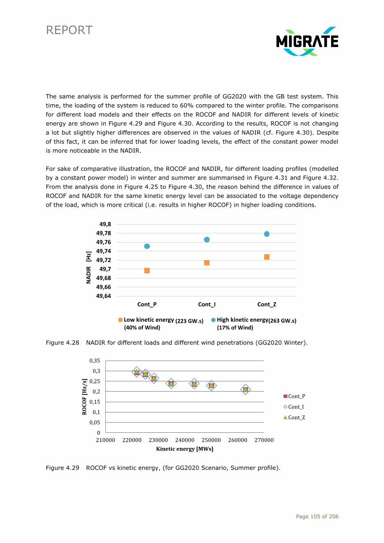
REPORT
Page 105 of 206
The same analysis is performed for the summer profile of GG2020 with the GB test system. This
time, the loading of the system is reduced to 60% compared to the winter profile. The comparisons
for different load models and their effects on the ROCOF and NADIR for different levels of kinetic
energy are shown in Figure 4.29 and Figure 4.30. According to the results, ROCOF is not changing
a lot but slightly higher differences are observed in the values of NADIR (cf. Figure 4.30). Despite
of this fact, it can be inferred that for lower loading levels, the effect of the constant power model
is more noticeable in the NADIR.
For sake of comparative illustration, the ROCOF and NADIR, for different loading profiles (modelled
by a constant power model) in winter and summer are summarised in Figure 4.31 and Figure 4.32.
From the analysis done in Figure 4.25 to Figure 4.30, the reason behind the difference in values of
ROCOF and NADIR for the same kinetic energy level can be associated to the voltage dependency
of the load, which is more critical (i.e. results in higher ROCOF) in higher loading conditions.
Figure 4.28 NADIR for different loads and different wind penetrations (GG2020 Winter).
Figure 4.29 ROCOF vs kinetic energy, (for GG2020 Scenario, Summer profile).
0
0,05
0,1
0,15
0,2
0,25
0,3
0,35
210000 220000 230000 240000 250000 260000 270000
RO
CO
F [
Hz/
s]
Kinetic energy [MWs]
Cont_P
Cont_I
Cont_Z
49,64
49,66
49,68
49,7
49,72
49,74
49,76
49,78
49,8
Cont_P Cont_I Cont_Z
NA
DIR
[H
z]
Low kinetic energy High kinetic energy(40% of Wind) (17% of Wind)
(223 GW.s) (263 GW.s)
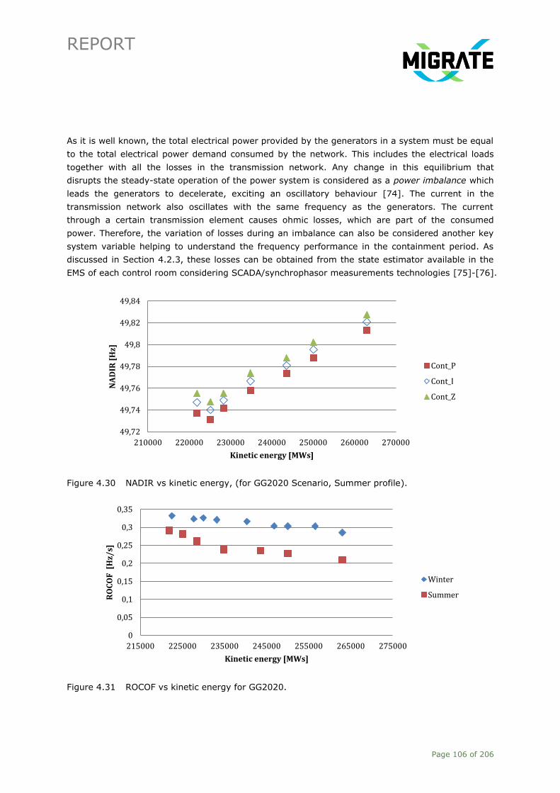
REPORT
Page 106 of 206
As it is well known, the total electrical power provided by the generators in a system must be equal
to the total electrical power demand consumed by the network. This includes the electrical loads
together with all the losses in the transmission network. Any change in this equilibrium that
disrupts the steady-state operation of the power system is considered as a power imbalance which
leads the generators to decelerate, exciting an oscillatory behaviour [74]. The current in the
transmission network also oscillates with the same frequency as the generators. The current
through a certain transmission element causes ohmic losses, which are part of the consumed
power. Therefore, the variation of losses during an imbalance can also be considered another key
system variable helping to understand the frequency performance in the containment period. As
discussed in Section 4.2.3, these losses can be obtained from the state estimator available in the
EMS of each control room considering SCADA/synchrophasor measurements technologies [75]-[76].
Figure 4.30 NADIR vs kinetic energy, (for GG2020 Scenario, Summer profile).
Figure 4.31 ROCOF vs kinetic energy for GG2020.
49,72
49,74
49,76
49,78
49,8
49,82
49,84
210000 220000 230000 240000 250000 260000 270000
NA
DIR
[H
z]
Kinetic energy [MWs]
Cont_P
Cont_I
Cont_Z
0
0,05
0,1
0,15
0,2
0,25
0,3
0,35
215000 225000 235000 245000 255000 265000 275000
RO
CO
F [
Hz/
s]
Kinetic energy [MWs]
Winter
Summer

REPORT
Page 107 of 206
This aspect becomes clearer considering the results shown in Figure 4.33. To capture the time
variation of the losses, two scenarios from GG2020, for winter and summer, are considered. And
the same fault as in the previous analysis is applied. In Figure 4.33a, the frequency of the COI is
depicted for winter and summer profiles, whereas the time derivative of the frequency of the COI
and the time variation of power losses are in Figure 4.33b and Figure 4.33c. The time derivative of
frequency of the COI (shown in Figure 4.33b) is derived by applying the derivative term of the
frequency of the COI (shown in Figure 4.33a). Note that when the derivative of the frequency of
the COI changes abruptly due to the imbalance, a similar pattern occurs for the ohmic losses. This
finding is in agreement with what was proven in [74], i.e. fluctuations of frequency of the COI are
dictated by the oscillations in the transmission network's ohmic losses.
Figure 4.32 NADIR vs kinetic energy for GG2020.
From the findings presented in this subsection, it is proposed to define a KPI for the assessment of
frequency performance in the containment period which maps information from key system
variables (i.e. inertia/kinetic energy, losses and load power) to well-known indicators (i.e.
ROCOF/NADIR). The procedure for implementation is explained in the following paragraphs.
Assumptions
The main assumptions which have been taken into account for the KPI for assessment of frequency
performance in the containment period are summarised as follows:
─ Synchronous generators are the main (predominant) source of system inertia in the frequency
containment period.
─ The loads are represented by a constant power model.
─ The droop of governors does not change.
─ PEIG connected at transmission level and only wind turbines type 3 and type 4 are considered.
These components do not possess a function for fast frequency response (to recreate the worst
case of ineffective or wrong participation in the frequency containment period).
49,68
49,7
49,72
49,74
49,76
49,78
49,8
49,82
210000 220000 230000 240000 250000 260000 270000
NA
DIR
Hz
Kinetic energy [MWs]
Winter
Summer
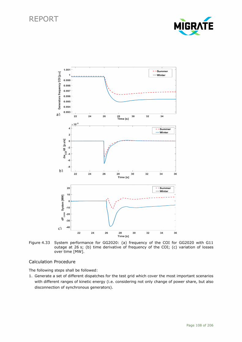
REPORT
Page 108 of 206
Figure 4.33 System performance for GG2020: (a) frequency of the COI for GG2020 with G11
outage at 26 s; (b) time derivative of frequency of the COI; (c) variation of losses over time [MW].
Calculation Procedure
The following steps shall be followed:
1. Generate a set of different dispatches for the test grid which cover the most important scenarios
with different ranges of kinetic energy (i.e. considering not only change of power share, but also
disconnection of synchronous generators).
a)
c)
b)

REPORT
Page 109 of 206
─ These set of dispatches can be used as the input to the procedure shown in Figure 4.5 and
Figure 4.10.
2. For each dispatch, compute the ROCOF and NADIR based on the frequency of the COI in the
system, which can be used to determine the trend of ROCOF/NADIR vs the level of system
kinetic energy.
3. For each dispatch, calculate the Sum of Maximum Active Power Deviation (SMAPD) of load and
losses, which reflects the effect of the active power consumption in the system on the system
active power balance, according to the following procedure:
─ Step1: record the time series (for the considered simulation time window) of the losses and
active power demand in the system.
─ Step2: SMAPD is the sum of the maximum values of active power load and losses
(aggregated system generation output) throughout the power system with respect to their
pre-disturbance value (before the occurrence of imbalance). The calculation of the SMAPD
can be performed in the same time window of calculation of the ROCOF, i.e. 0.5 sec after the
occurrence of the imbalance.
─ Step3: create the characteristic curve of SMAPD vs level of system inertia/kinetic energy.
4. Use the obtained mappings from previous steps 2 and 3, to assess the frequency performance
in the frequency containment period. For instance, if a given dispatch is planned for a given
loading condition, then, from the relational curves, the operator can estimate whether the
corresponding values of ROCOF/NADIR respect the thresholds defined in its grid code
requirements.
KPI implementation with the GB Test System
The calculation procedure described in the previous paragraphs has been implemented in the GB
test system for different scenarios (2016 as baseline, GG2020 and GG2030). All the analysis in this
subsection is applied for the system with the same conditions as previously:
─ Season: Summer, i.e. load peak at 60%.
─ Topological change: No.
─ Event: Generator outage representing 7% of the total system generation.
The first part of this KPI implementation is to obtain the mapping from system kinetic energy into
ROCOF/NADIR as shown in Figure 4.34 and Figure 4.35. It means, a set of feasible dispatches
covering different wind penetration levels is obtained and based on that, all ROCOF/NADIR values
are calculated and depicted.
As shown in Figure 4.34 and Figure 4.35, the blue points are related to the baseline scenario which
has more synchronous generators with less wind (i.e. wind penetration from 5 to 15%), the red
values are related to the GG2020 scenario (wind penetration from 15% to 40%) and the green
values are related to the GG2030 scenario (60% to 78% of wind penetration). Since most of the
synchronous generators are in service in the baseline scenario, more variety of feasible kinetic
energy is obtained for this case. From a simple visual inspection of the mapping trends for different
scenarios of the GB system, we can observe that the baseline scenario shows a more flat
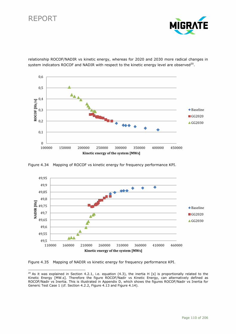
REPORT
Page 110 of 206
relationship ROCOF/NADIR vs kinetic energy, whereas for 2020 and 2030 more radical changes in
system indicators ROCOF and NADIR with respect to the kinetic energy level are observed20.
Figure 4.34 Mapping of ROCOF vs kinetic energy for frequency performance KPI.
Figure 4.35 Mapping of NADIR vs kinetic energy for frequency performance KPI.
20 As it was explained in Section 4.2.1, i.e. equation (4.3), the inertia H [s] is proportionally related to the Kinetic Energy [MW.s]. Therefore the figure ROCOF/Nadir vs Kinetic Energy, can alternatively defined as ROCOF/Nadir vs Inertia. This is illustrated in Appendix D, which shows the figures ROCOF/Nadir vs Inertia for Generic Test Case 1 (cf. Section 4.2.2, Figure 4.13 and Figure 4.14).
0
0,1
0,2
0,3
0,4
0,5
0,6
100000 150000 200000 250000 300000 350000 400000 450000
RO
CO
F [
Hz/
s]
Kinetic energy of the system [MWs]
Baseline
GG2020
GG2030
49,5
49,55
49,6
49,65
49,7
49,75
49,8
49,85
49,9
49,95
110000 160000 210000 260000 310000 360000 410000 460000
NA
DIR
[H
z]
Kinetic energy of the system [MWs]
Baseline
GG2020
GG2030
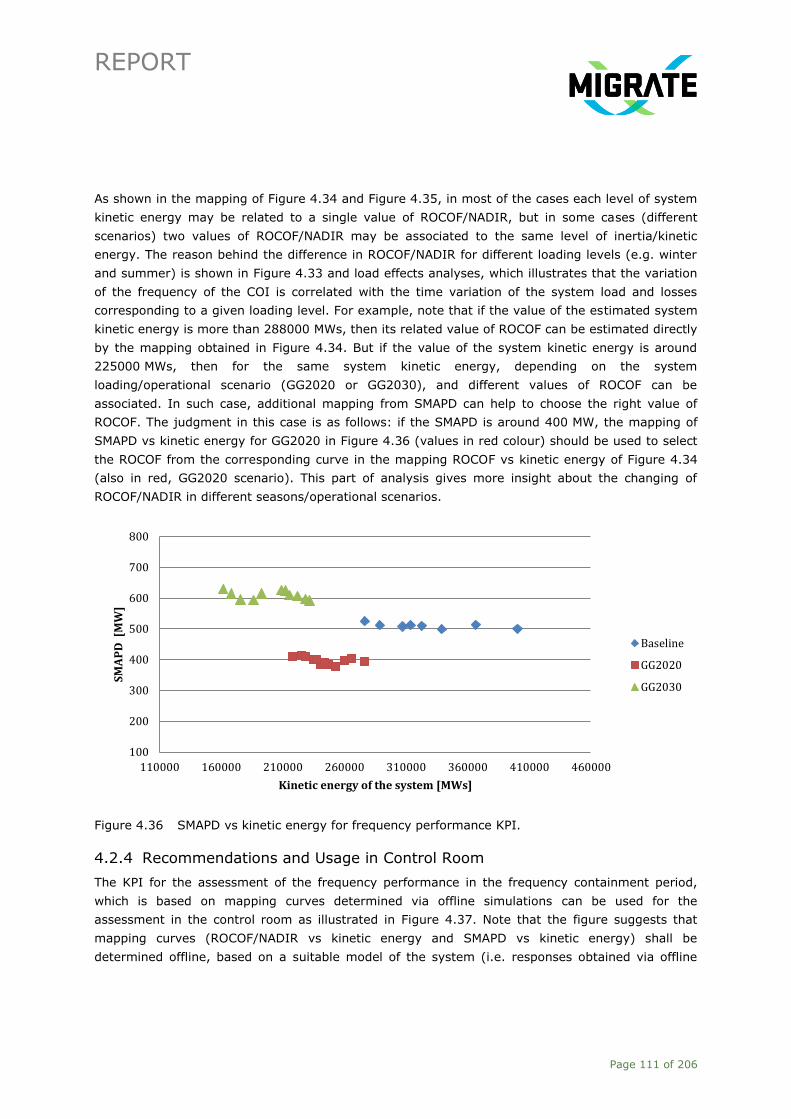
REPORT
Page 111 of 206
As shown in the mapping of Figure 4.34 and Figure 4.35, in most of the cases each level of system
kinetic energy may be related to a single value of ROCOF/NADIR, but in some cases (different
scenarios) two values of ROCOF/NADIR may be associated to the same level of inertia/kinetic
energy. The reason behind the difference in ROCOF/NADIR for different loading levels (e.g. winter
and summer) is shown in Figure 4.33 and load effects analyses, which illustrates that the variation
of the frequency of the COI is correlated with the time variation of the system load and losses
corresponding to a given loading level. For example, note that if the value of the estimated system
kinetic energy is more than 288000 MWs, then its related value of ROCOF can be estimated directly
by the mapping obtained in Figure 4.34. But if the value of the system kinetic energy is around
225000 MWs, then for the same system kinetic energy, depending on the system
loading/operational scenario (GG2020 or GG2030), and different values of ROCOF can be
associated. In such case, additional mapping from SMAPD can help to choose the right value of
ROCOF. The judgment in this case is as follows: if the SMAPD is around 400 MW, the mapping of
SMAPD vs kinetic energy for GG2020 in Figure 4.36 (values in red colour) should be used to select
the ROCOF from the corresponding curve in the mapping ROCOF vs kinetic energy of Figure 4.34
(also in red, GG2020 scenario). This part of analysis gives more insight about the changing of
ROCOF/NADIR in different seasons/operational scenarios.
Figure 4.36 SMAPD vs kinetic energy for frequency performance KPI.
4.2.4 Recommendations and Usage in Control Room
The KPI for the assessment of the frequency performance in the frequency containment period,
which is based on mapping curves determined via offline simulations can be used for the
assessment in the control room as illustrated in Figure 4.37. Note that the figure suggests that
mapping curves (ROCOF/NADIR vs kinetic energy and SMAPD vs kinetic energy) shall be
determined offline, based on a suitable model of the system (i.e. responses obtained via offline
100
200
300
400
500
600
700
800
110000 160000 210000 260000 310000 360000 410000 460000
SM
AP
D [
MW
]
Kinetic energy of the system [MWs]
Baseline
GG2020
GG2030

REPORT
Page 112 of 206
simulations have high resemblance with actual measured responses), for a selected number of
disturbances, each one evaluated for a number of dispatches (which entail variation of the power
share and system kinetic energy). Thus, a disturbance indicator (e.g. selecting the type of
disturbance that actually happens based on an alert signal from protection devices) can be used to
select the mapping curves, whereas information (actual kinetic energy, active power demand,
active power losses) from the energy Management System (EMS) is passed through the mapping
curves to estimate the ROCOF/NADIR. The procedure for determining the mapping curves was
introduced in Section 4.2.3. As illustrated in Figure 4.25 to Figure 4.36, the information
ROCOF/NADIR vs kinetic energy and SMAPD vs kinetic energy can be used in a complementary
manner to estimate the value of ROCOF/NADIR for a given loading level and generation dispatch.
Therefore, the decision block shown in Figure 4.37 suggests that the operators can also assess
what will happen with ROCOF in case an operational action (e.g. planned generator outage) is
taken and an imbalance is likely to occur in such operating conditions.
Start
for i=1:N disturbances
Offline simulation
Data extraction and processing
SCADA/
WAMS
ROCOF/NADIR vs kinetic energy
Yes
No
Ekin-sys
Pload
Ploss
Mapping Curve
Mapping Curve
SMAPD vs kinetic enrgy
Disturbance
indicator - IED1
2N
1
N2
Operational change?
EndOnline estimation
of ROCOF/NADIR
Figure 4.37 Implementation of the proposed frequency based KPI in control room. IED stands for intelligent electronic device.
The main limitation of this approach concerns with the use of a model implemented in a selected
software package. The lack of accuracy of the model to recreate the real behaviour can lead to

REPORT
Page 113 of 206
misleading results. Nevertheless, there has been a significant progress on model identification from
synchrophasor measurements [77]. Thus, the models used by operators can be improved and
updated regularly to ensure reliable (from numerical accuracy point of view) simulation results.
Moreover, the computing effort associated to the execution of offline simulations may be of concern
for large size systems. Nevertheless, the adoption of high performance computing in power system
simulation software packages can help to significantly reduce the computing time [78], [79].
A reliable estimator of the system kinetic energy is needed. An approach to estimate the kinetic
energy from synchrophasor data is explored in WP2 of MIGRATE. The estimation of total load active
power demand and active power losses can be done based on the state estimator, which is usually
based on SCADA measurements (1 sample per 2-6 seconds [75]). However, recent proposals have
been made to also consider synchrophasor measurements by sampling each 200 to 500 ms [76].
4.2.5 Validation with the Irish System
This section describes EirGrid’s assessment of the new frequency stability KPI in the Irish system.
The assumptions, methodology, and outcomes of the assessment are discussed next.
Assumptions
The only source of reserve in the system comes from synchronous generators. This assumption is
consistent with work performed for the KPI development and the assessment in the GB system,
therefore it is used here to harmonise the analysis and compare outcomes. However, it must be
noted that this assumption neglects the possible contribution to frequency control from PE based
sources like batteries, wind, PV, flywheels, HVDC, etc. It is understood that these effects will be
assessed in Task 1.6 as part of the development of mitigation measures.
The operation of ROCOF protection relays normally installed in embedded generators was not
included in the simulations. This simplification was made to facilitate a better observability and
understanding of the system dynamics following a large power imbalance. Inclusion of these
protection relays would result in cascade tripping that will mask the physical behaviour of the
system. Similarly, Under-Frequency Load Shedding (UFLS), Interruptible Load (IL) and Demand
Side Management (DSM) schemes have not been included in the simulations
Methodology
System Demand
In order to assess the relationship between frequency stability and the system loading, two
demand scenarios are assessed side by side: Winter Peak (5 GW) and Summer Peak (4 GW).
Network topology and synchronous generation capacity remain the same in both operational cases.
HVDC interconnector flows are set to 350 MW import in the Winter Peak cases and 350 MW export
in the Summer Peak cases.

REPORT
Page 114 of 206
Development of Scenarios
In order to systematically assess the impact of increased levels of PE based generation in the Irish
system, a series of scenarios have been developed using the Baseline case described in Section
3.3.3. Each simulation series is comprised of 12 distinct sub-cases in which the level of PE based
generation (i.e. wind) is increased from 0 MW to 2750 MW in steps of 250 MW. The wind turbine
generators (WTG) are set at their maximum rated output in all scenarios and the incremental wind
output is introduced by scaling the number of WTGs in the model.
In total, 24 scenarios are assessed: 12 for Winter Peak and 12 for Summer Peak. In each scenario,
the generation output of the synchronous machines is reduced appropriately to balance the fixed
level of demand. When the output of a synchronous machine drops below its rated minimum load,
this machine is taken offline and its remaining output is re-dispatched to other online units.
Common to all scenarios is the output of “Longpoint AD2” synchronous generator (425 MW), which
is tripped to generate the power imbalance in the simulations. Therefore, the dispatch of this unit is
left constant to assess all simulation results in equal terms. The dispatch of this machine
represents 8.5% of the Winter Peak load and 10.6% of the Summer Peak load.
A detailed breakdown of all generation dispatches (Summer and Winter) with the output of each
unit is tabulated in Appendix B.2. In these tables, each column represents a single generation
dispatch scenario. For each synchronous machine, an “X” means that the generator is offline
whereas a number indicates the dispatched output in MW.
The generation dispatches developed for Winter Peak are illustrated in Figure 4.38. This graph
shows the kinetic energy of the system as a function of the wind generation. A description of the
dispatches follows:
─ For scenarios #1 (0 MW wind) to #4 (750 MW wind), the combined wind output is not too
significant and it can be accommodated by simply reducing the output of some synchronous
generators, but no unit is taken off-line. As a result, Figure 4.38 shows that the system kinetic
energy does not change (i.e. the same rotating mass is present in these four cases).
─ Scenarios #5 (1000 MW wind) to #12 (2750 MW wind) represent cases where the increasing
level of wind generation displaces synchronous machines, which have to be taken offline. Now
the graph shows that the system kinetic energy is continuously falling, as expected. The rate at
which the kinetic energy drops on each scenario depends on the size and characteristics of the
unit(s) that is taken offline at each step.
The generation dispatches developed for the Summer Peak case follow similar trends as the Winter
Peak and they are not illustrated here for simplicity. It should be noted that the selected scenarios
did not attempt to follow an economic dispatch. However, a “pseudo” merit-order approach was
assumed, based on knowledge of the Irish system, whereby the most efficient and must-run plant
was decommissioned last.
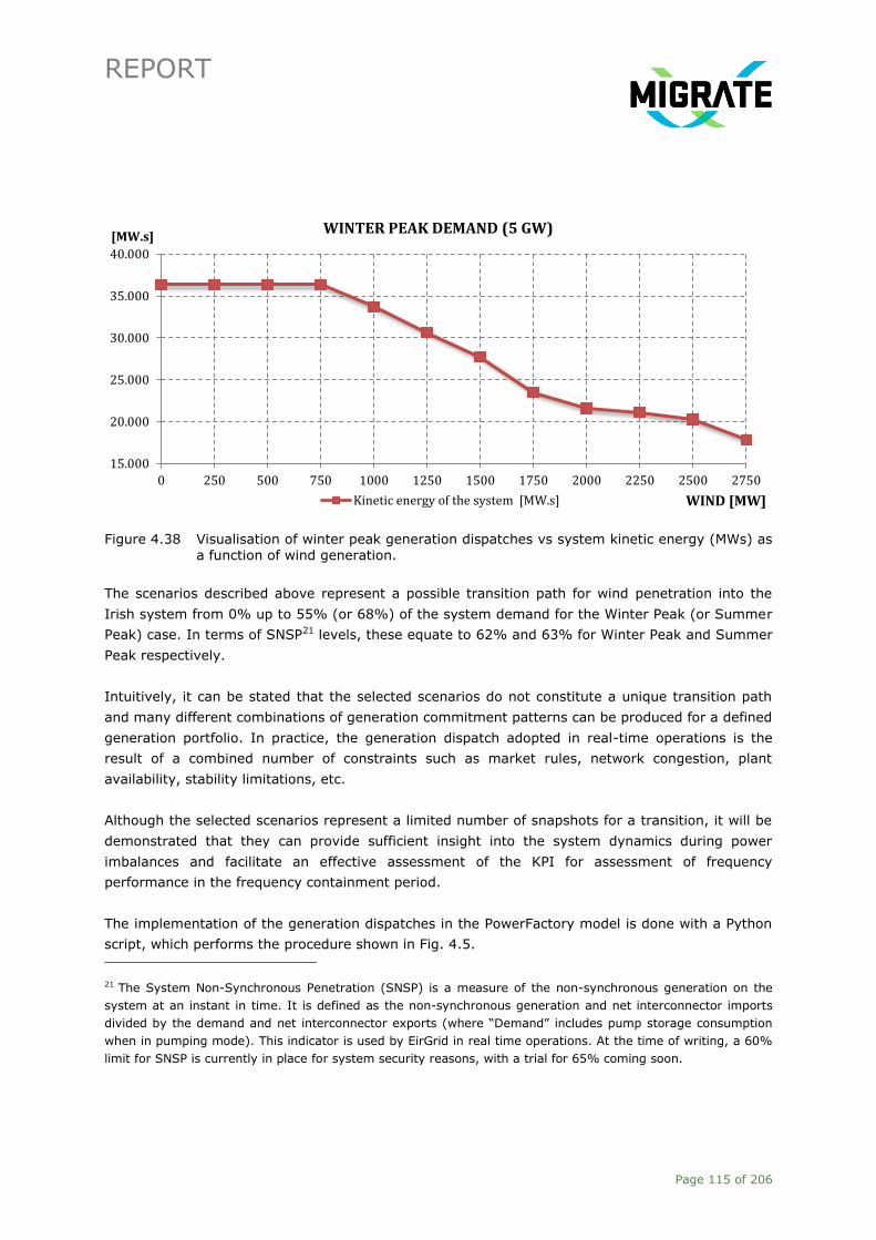
REPORT
Page 115 of 206
Figure 4.38 Visualisation of winter peak generation dispatches vs system kinetic energy (MWs) as a function of wind generation.
The scenarios described above represent a possible transition path for wind penetration into the
Irish system from 0% up to 55% (or 68%) of the system demand for the Winter Peak (or Summer
Peak) case. In terms of SNSP21 levels, these equate to 62% and 63% for Winter Peak and Summer
Peak respectively.
Intuitively, it can be stated that the selected scenarios do not constitute a unique transition path
and many different combinations of generation commitment patterns can be produced for a defined
generation portfolio. In practice, the generation dispatch adopted in real-time operations is the
result of a combined number of constraints such as market rules, network congestion, plant
availability, stability limitations, etc.
Although the selected scenarios represent a limited number of snapshots for a transition, it will be
demonstrated that they can provide sufficient insight into the system dynamics during power
imbalances and facilitate an effective assessment of the KPI for assessment of frequency
performance in the frequency containment period.
The implementation of the generation dispatches in the PowerFactory model is done with a Python
script, which performs the procedure shown in Fig. 4.5.
21 The System Non-Synchronous Penetration (SNSP) is a measure of the non-synchronous generation on the
system at an instant in time. It is defined as the non-synchronous generation and net interconnector imports
divided by the demand and net interconnector exports (where “Demand” includes pump storage consumption
when in pumping mode). This indicator is used by EirGrid in real time operations. At the time of writing, a 60%
limit for SNSP is currently in place for system security reasons, with a trial for 65% coming soon.
15.000
20.000
25.000
30.000
35.000
40.000
0 250 500 750 1000 1250 1500 1750 2000 2250 2500 2750
[MW.s]
WIND [MW]
WINTER PEAK DEMAND (5 GW)
Kinetic energy of the system [MW.s]

REPORT
Page 116 of 206
Dynamic Simulations
The main objective of this assessment is to understand the dynamic behaviour of the system
frequency during a severe power imbalance and how it is affected by the increased penetration of
PE based generation (and associated displacement of conventional generation plant). This
investigation is performed by running RMS time-domain simulations for all scenarios, subject to the
same disturbance.
For the purposes of this assessment, the trip of 425 MW of synchronous generation (“Longpoint
AD2” unit) is defined as the reference disturbance. This event has been selected for the following
reasons:
─ It represents the loss of the largest single infeed in the selected scenarios. Therefore, it
generates the largest power imbalance.
─ It results in the disconnection of the largest amount of inertia in a single event. Therefore, it
reduces the ability of the system to slow down the falling frequency.
The main variable of interest in these simulations is the frequency output for each synchronous
generator. These frequency traces are combined into a centre-of-inertia (COI) as described in
Section 4.2.1. The frequency NADIR and ROCOF conclusions apply to the combined COI for the
entire system.
Other steady-state variables like circuit loading and generation dispatch are also monitored and
extracted from the PowerFactory simulations as described in Section 4.2.2.
The above processes are automated with two scripts:
─ DataExtraction_Freq.py: Python scrip that runs through the defined list of scenarios in
PowerFactory, performs the dynamic simulation for each scenario and extracts the selected
variables into csv output files.
─ RoCoF_Nadir.m and SS_proces.m: Matlab scripts that post-process the PowerFactory simulation
outputs and generate the indices described in Section 4.2.1.
Simulation findings
This subsection presents the outcome of the dynamic simulations performed with the Irish system
model. Analysis of the results suggests slightly higher values of ROCOF and lower frequency NADIR
in the Summer Peak scenarios than in the equivalent Winter Peak scenarios. This behaviour is
expected and can be explained by the reduced number of synchronous generators required to meet
the lower load. The summer scenarios have less inertia and less load damping than the winter ones,
therefore the frequency excursions are more pronounced in terms of rate of decay and amplitude.
For simplicity, this section will only present the Summer Peak results. The Winter Peak results
follow the same trend, but they are less severe.
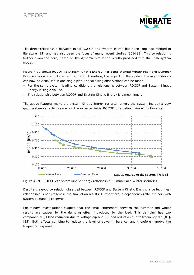
REPORT
Page 117 of 206
The direct relationship between initial ROCOF and system inertia has been long documented in
literature [12] and has also been the focus of many recent studies [80]-[83]. This correlation is
further examined here, based on the dynamic simulation results produced with the Irish system
model.
Figure 4.39 shows ROCOF vs System Kinetic Energy. For completeness Winter Peak and Summer
Peak scenarios are included in the graph. Therefore, the impact of the system loading conditions
can now be visualised in one single plot. The following observations can be made:
─ For the same system loading conditions the relationship between ROCOF and System Kinetic
Energy is single-valued.
─ The relationship between ROCOF and System Kinetic Energy is almost linear.
The above features make the system Kinetic Energy (or alternatively the system inertia) a very
good system variable to ascertain the expected initial ROCOF for a defined size of contingency.
Figure 4.39 ROCOF vs System kinetic energy relationship, Summer and Winter scenarios.
Despite the good correlation observed between ROCOF and System Kinetic Energy, a perfect linear
relationship is not present in the simulation results. Furthermore, a dependency (albeit minor) with
system demand is observed.
Preliminary investigations suggest that the small differences between the summer and winter
results are caused by the damping effect introduced by the load. This damping has two
components: (i) load reduction due to voltage dip and (ii) load reduction due to frequency dip [84],
[85]. Both effects combine to reduce the level of power imbalance, and therefore improve the
frequency response.
0,100
0,300
0,500
0,700
0,900
1,100
1,300
18.000 23.000 28.000 33.000 38.000
RO
CO
F [
Hz/
s]
Kinetic energy of the system [MW.s] Winter Peak Summer Peak

REPORT
Page 118 of 206
This observation aligns with the analytical expression (equation (4.6)) derived from the well know
swing equation under the assumption of no load damping. The linearity of the equation disappears
if a damping coefficient is added to reflect the load dependency with voltage and frequency.
Further research work is recommended to better understand this process.
In practice, the use of equation (4.6) in Ireland has shown very good correlation with
measurements of actual system disturbances. It is acknowledged that the equation lacks
information about the inertia of the load and associated damping effects, therefore the results are
generally on the conservative side. However, this provides and inherent safety margin for the
secure and reliable operation of the system.
Caveats
The dynamic studies presented in this section have been based on a limited number of scenarios,
therefore this cannot be interpreted as an exhaustive study into the dynamic performance of a real
power system. It is worth highlighting some of the assumptions and simplifications made in the
analysis and their impact on results:
─ Generic models were used to represent the governors and AVR controllers for all synchronous
generators. These models were tuned to produce typical and realistic responses based on
experience. However, their response has not been validated against system disturbances. The
results, thus, cannot be interpreted as a true reflection of the performance of the Irish system.
─ A simplified dynamic representation of the load has been adopted for this analysis. Accurate
load dynamic models are currently under development within the MIGRATE project (in Task 1.3),
but not yet available at the time of writing. Some sensitivity analyses were performed with the
Irish model to investigate the impact of the load representation (dynamic and static). These
analyses showed that the load representation had a distinct impact on the frequency response
of the system. However, the trends shown in Figure 4.38 and Figure 4.39 were not altered. This
finding emphasises the need for accurate dynamic load modelling but it does not contradict the
conclusions related to correlations between initial ROCOF and System Kinetic energy.
─ The operation of ROCOF protection relays normally installed in embedded generators was not
included in the simulations. This simplification was made to facilitate a better observability and
understanding of the system dynamics following a large power imbalance. Inclusion of these
protection relays would result in cascade tripping that will mask the physical behaviour of the
system. Therefore, the conclusions related to the linear relationship between initial ROCOF and
Kinetic Energy are only applicable outside the range of operation of these protection relays. The
goal is to avoid tripping of generation, either by adjusting the protection settings or by adopting
an alternative protection scheme.
─ Similarly, Under-Frequency Load Shedding (UFLS), Interruptible Load (IL) and Demand Side
Management (DSM) schemes have not been included in the simulations. These schemes are
designed to reduce the power imbalance and arrest the falling frequency. However, they are not
fast enough to influence the initial ROCOF. Therefore, the conclusions from the studies are still
valid.

REPORT
Page 119 of 206
─ The only source of mitigation to the falling of frequency in the model comes from synchronous
generators. This assumption is consistent with the context (i.e. reduction of system inertia and
no participation of PE interfaced sources) defined in D1.1 [2] for frequency performance in the
containment period work performed for the KPI development (Section 4.2.3) and the
assessment in the GB system, therefore it is used here to harmonise the analysis and compare
outcomes. However, it must be noted that this assumption neglects the possible contribution to
frequency control from PE based sources like batteries, wind, PV, flywheels, HVDC, etc. Some of
these technologies could act fast enough to affect the initial ROCOF, therefore the relationship
between ROCOF and System Kinetic Energy may change. The challenge will be to identify how
much of that new source of restoring power (in addition to the inertial response from
synchronous machines) is required to maintain system stability in conditions of very low system
inertia. It is understood that these effects will be assessed in Task 1.6 as part of the
development of mitigation measures.
─ Generic models for wind generation were developed by Energynautics as part of the MIGRATE
project. These WTG models were integrated in the PowerFactory model of the Irish system.
Parameter setting and configuration for these models were advised by Energynautics. From a
limited number of tests performed in the Irish system model, the response of the generic WTG
models was in line with typical performance requirements in Grid Codes.
The above assumptions and simplifications need to be considered when analysing the results.
Indeed, the study findings and conclusions presented in this section must be interpreted from a
qualitative, rather than quantitative, point of view.
Conclusions and Recommendations
This section has presented EirGrid’s assessment of the performance and suitability of the new KPI
proposed for assessment of frequency stability in the frequency containment period in Section
4.2.3.
Dynamic simulations of the Irish system have been performed to assess the suitability of the new
KPI. While based on a limited number of scenarios, the studies have provided adequate insight into
the system dynamics during the frequency containment period.
Kinetic Energy has shown to be directly related to the initial ROCOF and it is currently used in
Ireland with great success. However, as the level of PE based generation increases, the depleted
system inertia will cause the frequency to fall too fast for conventional controllers to act in time.
Therefore, fast delivery of power will be required in order to arrest the rapid falling frequency. The
speed of operation of this reserve (either POR of FFR) needs be accounted for in a reliable and
robust KPI.
A complex interaction between system inertia, FFR and POR is expected. The main challenge will be
to understand and capture those interactions into a simple, concise and reliable indicator. It is
recommended that further research work is undertaken in this direction to derive a reliable KPI

REPORT
Page 120 of 206
that reflects the key behaviour of the system during the frequency containment period. This KPI
should be robust enough to predict initial ROCOF and, most importantly, frequency Nadir.
Given the small size of the Irish system, locational variations of inertia are not significant. This,
however, will not apply to large interconnected systems like the pan-European grid. It is
recommended that further research work is performed to understand the propagation of frequency
instabilities through large networks and to investigate the concept of regional inertia [66].
4.3 KPI for Large-Disturbance Rotor Angle Stability
4.3.1 Introduction
Large-disturbance rotor angle stability (also known as transient stability) concerns the ability of the
synchronous generators of an interconnected power system to remain in synchronism after being
subjected to a large disturbance, such as a three-phase short circuit on a transmission line or a tie-
line tripping [3]. When such a disturbance occurs, the equilibrium between the mechanical and the
electrical torque in each synchronous generator is altered, resulting in large excursions (swings) of
the rotor angles (which are influenced by the non-linear power-angle relationship). If the angular
swings are not too large and attenuated, the system can reach a (new) steady-state operation
condition again and is considered stable. Unstable conditions occur when some generators lose
their synchronism with other generators due to too large or increasing angular swings, which is an
indication that the system cannot absorb the kinetic energy corresponding to the rotor speed
differences [3].
Large-disturbance rotor angle instability can lead to generator outages, load shedding, tripping of
major transmission lines and even blackouts. Significant research efforts have been devoted to
develop methods to continuously monitor and estimate the degree of large-disturbance rotor angle
stability in systems dominated by synchronous generators [86], [87]. Nevertheless, the massive
integration of renewable generation involves a phase out of synchronous generators, challenging
the large-disturbance rotor angle stability of the remaining ones, which have to cope with the
variability of operating conditions introduced by renewable generation22.
The critical clearing time [88], maximum angle difference [89], and area-based centre-of-inertia
referred rotor angle [90], constitute the most widely used indicators in the current state-of-the-art
on assessment of the impact of increasing penetration of renewables on large-disturbance rotor
angle stability. These indicators are determined from signal records (generated via offline time
domain simulations or obtained from synchrophasor measurements), and there is evidence that
these indicators can still be suitable, cf. the application of the critical clearing time in [91].
Therefore, a comparative assessment among them is out of the scope of the work presented in this
section. The maximum angle difference indicator is chosen in this work due to the reduced
22 The massive penetration of power electronic interfaced renewable generation entails a reduction of the system inertia and the short circuit capacity levels. This is also reflected in the severity of fault currents.

REPORT
Page 121 of 206
computing effort and conceptual simplicity. Any of the other two indicators can be used in the
proposed KPI as well. Alternative indicators, determined by using simplified models and usually
without performing time domain simulations (e.g. equal area criterion [12]) have been also
proposed in existing literature. They only allow providing a qualitative assessment (intuitive
insight) and therefore are not considered in this work.
The second fundamental question to be answered is how to structure a KPI which helps in
quantifying the effect of the change of one or more key variables on the distance to large-
disturbance rotor angle instability. In order to evaluate such a KPI, two things are needed:
1. Large-disturbance rotor angle stability margin. It is quantified based on the acceptable
maximum angle difference ∆𝛿max (like 180 degrees [3]), namely:
where ∆𝛿 is the angle difference between any two generators. This factor defines the extent of
large-disturbance rotor angle stability, and enables system operators to estimate the distance
from the current operation condition to the instability border (namely ∆𝛿max 180). The margin
can also be defined by using an alternative expression, like (360 − ∆𝛿)/(360 + ∆𝛿 ) in [89].
2. Mapping from key variables to large-disturbance rotor angle stability margin, that is to say, if
key variables are measured, how could it be possible to know the maximum angular difference?
Unlike the assessment of frequency performance due to the inertial response in the frequency
containment period (which is dominated by the level of inertia in the system), the non-linear
nature of large-disturbance rotor angle stability and the influence of more than one or two
variables does not allow defining a simple mapping curve. Therefore, an estimation method is
needed to infer the maximum angle difference associated to a set of selected key variables. The
most popular methods to estimate large-disturbance rotor angle stability margin come from the
field artificial intelligence [92], [93]. Particularly a random forest consisting of Decision Trees
(DTs) is adopted here because of the good interpretability (or transparency) and easy
implementation. Other methods, like support vector machine based regressor, can also be used.
Decision trees estimate the angle of any generator selected by the operators, and calculate the
maximum angle difference, namely max∆𝛿, and then estimate the margin. Nevertheless, the
research effort devoted to this section is focused on two essential and aspects:
─ investigating what could be the smallest set of key system variables needed to estimate the
maximum angular difference in a system with high penetration levels of renewables;
─ jointly tackling the problem of key variable selection and the design of the selected artificial
intelligence method. So far, the problem of key variable selection has been treated
separately in existing literature. The method described below can be easily applied for cases
in which other artificial intelligence methods are preferred. From a practical point of view,
the operator can select all variables monitored with available PMU devices. At least, the bus
voltage magnitude and angle can be selected as candidate key variables for the decision
tree The application of MVMO will indicated which variables are the most representative
Margin = ∆𝛿max −max∆𝛿 (4.10)

REPORT
Page 122 of 206
(high observability). Data series (time responses) collected with available PMU devices can
be used instead of data generated via offline simulations.
The remainder of this section reports the work for selecting key variables to estimate large-
disturbance rotor angle stability of power systems with high penetration of renewable generation.
Simply put, the estimation accuracy that can be achieved by using decision trees is used to
investigate the influence of system variables on large-disturbance rotor angle stability. A weight
factor is given to each variable. An optimisation method, Mean–Variance Mapping Optimisation
(MVMO), is adopted to optimise weight factors to minimise the errors of decision trees. In the list
of weight factors corresponding to the minimum error, the variables with the largest weight factors
are considered as the key variables. Decision trees built with key variables are considered as the
optimal performance trees and are used to estimate large-disturbance rotor angle stability.
Next, the background of decision trees and MVMO is first introduced. Then the proposed method of
selecting key variables to estimate large-disturbance rotor angle stability is described. The method
is first demonstrated on a modified version of the generic test case 2, which was introduced in
Section 3.2.4, to illustrate its implementation. Finally, the method is tested on GB system to
ascertain its feasibility and efficiency when applied to a larger size system.
4.3.2 Decision Trees Background
Decision Trees are one of the most popular classifiers, which are used in various disciplines such as
statistics, machine learning, pattern recognition, data mining, etc. Decision trees are successful
because they provide a clear, documentable and discussible model of how the classification is made
[94], [95]. The model maps a new observation into a most appropriate class, whose average of
outputs is considered as the output of this new observation.
As shown in Figure 4.40, a decision tree is a graphical description of a well-defined decision
problem, which is composed of a root node, branches, internal nodes and leaves [94]. The root
node is the starting point of the tree, without any incoming branch. The internal nodes constitute
nodes with incoming branches and outgoing branches. Each internal node splits its sample set into
two or more sub-classes according to a certain splitting criterion. A branch is a connection
descending from an upper (parent) node to a lower (child) node. The nodes with incoming
branches but without outgoing branches are called leaf nodes. Each leaf node is assigned a target
value or a decision as its output. Here, the maximum angular difference is considered as the output
of leaf node. Essentially, a path from a root node to a leaf node is a series of if-else rules, which
make the internal logic and reasoning process easy to comprehend. A decision tree is built in the
way that the training samples are recursively split into smaller left and right groups in a top-down
manner by selecting a certain splitting at a node, until the stopping criterion is met.

REPORT
Page 123 of 206
Figure 4.40 Structure of a decision tree.
When a new observation is collected, it will be navigated from a root node down to a leaf node,
according to the splitting used at each node. The leaf node includes a set of samples who have
similar characteristics to this new observation. Therefore the average of outputs of these similar
samples is considered as approximately the estimation for the new observation. As far as large-
disturbance rotor angle stability is concerned, the output of a leaf node is defined as the average of
maximum angle differences associated to L samples in this leaf node [96].
where:
∆𝛿est = the estimated maximum angle difference for the new observation
l = the lth sample in the leaf node
The key task in the design of the decision trees is to select the proper splitting at each node so that
the training samples are classified. Here, the method named CART is selected because it tends to
build simple binary trees which can clearly show the relationship between measured system states
and maximum angular differences [96].
Like any artificial intelligence method, good accuracy of decision trees requires enough training
samples (i.e. sets of numerical values of the system variables used as inputs of the decision tree).
With the samples obtained by using an accurate model in power system simulations, decision trees
can identify the link between system states and large disturbance rotor angle stability. But
numerous samples will slow down the computing speed of the decision trees. Therefore, the
training (exploration) and testing (exploitation) of decision trees should be well balanced. Moreover,
during the training process, the selection of input variables also has a big influence on the accuracy
of decision trees. Here, this topic is dealt with by using an optimisation method, MVMO, which is
described next.
∆𝛿est =∑ ∆𝛿𝑙𝐿𝑙=1
𝐿 (4.11)

REPORT
Page 124 of 206
Yes
No
Start
Initialize algorithm and optimization problem parameters
Normalize optimization variables in vector x to range [0, 1]
Fitness evaluation by using de-normalized variables
StopTermination criteria satisfied?
---
Ranking Fitness x1 x2 ... xD
1st best
2nd best
...
F1
F2
Last best FA
Mean --- ...
Shape ---
d-factor ---
1x
1s2x Dx
2s Ds...
1d 2d Dd...
Optimization
Variables
Store n-best population
Parent assignment
The first ranked solution xbest is chosen as parent
Offspring generation
Selection: Select m (m<D) dimensions of x
For selected m dimensions, calculation
of h-function variables si1, si2 and x1
Mapping:
i
i1
i2
x
s
s
*i=x rand
1
0
newix
1
Crossover: Use the values of xbest for the
remaining dimensions of x
Offspring
generation
Figure 4.41 Flow chart of MVMO.

REPORT
Page 125 of 206
4.3.3 Background of MVMO
MVMO belongs to the family of evolutionary optimisation algorithms. Its main feature is its unique
search mechanism for exploring the possible values of the optimisation variables within a
normalised range of search space. It also adopts a single parent-offspring approach (i.e. a single
solution vector is iteratively evolved). Moreover, the n-best solution vectors achieved so far are
stored and ranked based on their fitness value in an archive, which is recurrently updated. The
mean and variance of each optimisation variable within the best solution vector achieved so far are
computed from the archive and used to guide the generation of new solutions. The first ranked
solution in the archive is selected as starting point to generate a new solution. Next, a non-linear
mapping function is applied to selected optimisation variables. The selection is based on a random-
sequential approach. The mean and variance of each selected optimisation variable are inputs to
the mapping function, which generates new values for these variables. The non-linear shape of the
mapping function is automatically adapted over the iterations to move from search exploration
(generating solutions in different regions of the search space) to search exploitation (intensifying
the search within a region of the search space in which the optimum solution is located). As a
result, MVMO exhibits fast convergence characteristics and efficiently avoids premature
convergence [97], [98]. The overall process is illustrated in Figure 4.41. The iterative process is
automatically executed until a predefined termination criterion (e.g. a fixed number of fitness
evaluations) is fulfilled.
4.3.4 Outline of the Proposed Method of Selecting Key Variables
The selection of key variables is shown in Figure 4.42. Based on operational experience, a group of
L candidates of key variables (which can be directly obtained or derived from phasor measurement
units, like generator output power) is defined. Then, considering a combination of uncertainties
defining different operating conditions (e.g. different generator dispatch and load profile, different
fault clearing times), training samples are generated. An initial weight factor is given to each
candidate variable. Then, a group of decision trees is built and its accuracy is tested. For this
purpose, the accuracy error is defined as the sum of deviations between estimated and simulated
maximum angular differences associated to a set of samples.
where:
∆𝛿est.𝑘 : the estimated angle difference
∆𝛿sim.𝑘 : the simulated angle difference
k : kth test, k=1,2,…, K
The errors and trees are sent to MVMO, which will optimise the weight factor for each candidate
variable, and then rebuild the decision trees and test them again until the stopping criterion (e.g.
an accuracy threshold) is met. The above optimisation of weight factor can be described by the
model in the following equation:
Err = ∑(max∆𝛿est.𝑘 −max∆𝛿sim.𝑘)
𝐾
𝑘=1
(4.12)

REPORT
Page 126 of 206
subject to:
where L is the total number of weight factors; 𝑤𝑙min and 𝑤𝑙
max are respectively 0 and 1 in the work
carried out in this section.
Finally, MVMO method provides a sequence of weight factors from the largest to the smallest. The
system operator can decide how many variables are selected. Selecting more variables means
more measurements and smaller estimation errors of decision trees. Selecting less variables means
less measurements and larger errors of decision trees.
Figure 4.42 Key variable selection.
From Figure 4.42, when obtaining key variables (loop MVMO-build decision trees), a group of
decision trees are built. For sake of illustration, Figure 4.43 shows one part of a designed decision
tree, taking generic test case 2 as example. Overall, it is worth pointing out that decision trees
have rules that are built upon input-output data obtained from simulations of the power system.
The rules constitute the knowledge extracted from the samples of inputs (e.g. generator speed S2,
bus voltage magnitude V9 and V5, etc.) and output (stability indicator, e.g. rotor angle margin,
which corresponds to the sampled inputs).
minimize Err (𝐖) (4.13)
𝐖 = [𝑤1, 𝑤2, , … , 𝑤L] (4.14)
𝑤𝑙min ≤ 𝑤𝑙 ≤ 𝑤𝑙
max , 𝑙 = 1, 2, … , L (4.15)
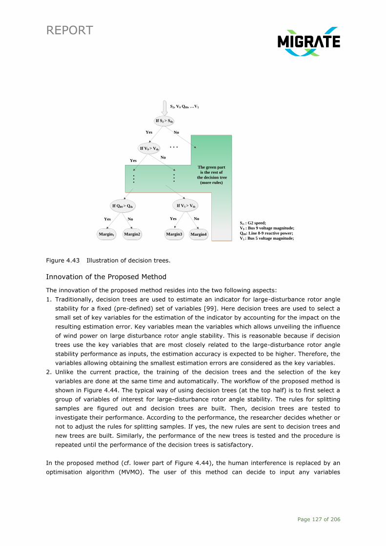
REPORT
Page 127 of 206
S2, V9 Q89, …V5
If S2 > Sth
Yes No
If V9 > Vth
Yes
Margin1
If Q89 > Qth
Margin2
YesNo
If V5 > Vth
Margin3
Yes
Margin4
NoNo
. . .
. . .
. . .
The green part
is the rest of
the decision tree
(more rules)
S2: : G2 speed;
V9 : Bus 9 voltage magnitude;
Q89: Line 8-9 reactive power;
V5 : Bus 5 voltage magnitude;
Figure 4.43 Illustration of decision trees.
Innovation of the Proposed Method
The innovation of the proposed method resides into the two following aspects:
1. Traditionally, decision trees are used to estimate an indicator for large-disturbance rotor angle
stability for a fixed (pre-defined) set of variables [99]. Here decision trees are used to select a
small set of key variables for the estimation of the indicator by accounting for the impact on the
resulting estimation error. Key variables mean the variables which allows unveiling the influence
of wind power on large disturbance rotor angle stability. This is reasonable because if decision
trees use the key variables that are most closely related to the large-disturbance rotor angle
stability performance as inputs, the estimation accuracy is expected to be higher. Therefore, the
variables allowing obtaining the smallest estimation errors are considered as the key variables.
2. Unlike the current practice, the training of the decision trees and the selection of the key
variables are done at the same time and automatically. The workflow of the proposed method is
shown in Figure 4.44. The typical way of using decision trees (at the top half) is to first select a
group of variables of interest for large-disturbance rotor angle stability. The rules for splitting
samples are figured out and decision trees are built. Then, decision trees are tested to
investigate their performance. According to the performance, the researcher decides whether or
not to adjust the rules for splitting samples. If yes, the new rules are sent to decision trees and
new trees are built. Similarly, the performance of the new trees is tested and the procedure is
repeated until the performance of the decision trees is satisfactory.
In the proposed method (cf. lower part of Figure 4.44), the human interference is replaced by an
optimisation algorithm (MVMO). The user of this method can decide to input any variables

REPORT
Page 128 of 206
(engineering judgment from operational experience) to the decision trees, together with initial
weight factors (defined in the range [0,1]). MVMO is responsible to optimise the weight factors to
reduce the errors of the decision trees. The new weight factors are sent to the decision trees again.
And MVMO continues to optimise them until the stopping criterion is satisfied. The list of weight
factors will tell the user what the key variables are, and at the same time, the decision trees
corresponding to the minimum error are considered as the finally trained trees.
4.3.5 Test Results with Generic Test Case 2
The proposed method is first illustrated on a variant of generic test case 2, namely the modified
version of generic test case 2 (cf. Section 3.2.4). Generator G1 is replaced by a wind turbine type 3.
G3 is selected as the reference generator. The angle of generator G2 is observed to investigate
large-disturbance rotor angle stability.
Figure 4.44 Innovation of the proposed method.
In the first step of designing decision trees, enough samples should be collected. In order to collect
samples, the following uncertainties are considered to generate different operation conditions.
─ Fault location. A three-phase short circuit fault is applied on different locations [1%, 50%, 99%]
in each of six transmission lines of generic test case 2 at different percentages of the line length.

REPORT
Page 129 of 206
─ Fault duration. Different fault durations, namely [0.35s, 0.36s, 0.37s, 0.38s, 0.39s, 0.40s,
0.41s, 0.42s, 0.43s, 0.44s, 0.45s], are considered to simulate the severity of fault.
─ Inertia constant of G2. This factor determines how quickly G2 accelerates/decelerates due to
the imbalance of electrical and mechanical torque. Two values, 3.3s and 3.4s are selected in
this part. It is worth pointing out that, due to the fact that the inertia constants of the
generators of the 9 bus system are small (<5 s), this small change in the value of the inertia
constant can cause the 9 bus system to transit from large-disturbance rotor angle stability to
large-disturbance rotor angle instability for some combinations of fault location and fault
duration.
The different fault locations will cause different power imbalances at the terminal of generator G2,
and thus influence its transient stability in a different way. Therefore, to better estimate the
transient stability of generator G2, the samples representing different fault locations are
incorporated in the training. Moreover, the inertia of generator G2 is closely related to the
accelerating speed of generator G2. Therefore, the uncertainties of these three elements are used
to create stable and unstable samples for decision trees. In total, 396 samples (combinations of 3
samples of fault location in 6 transmission lines, 11 samples of fault duration, 2 samples of inertia
constant of G2) are collected. Each of them is simulated in PowerFactory 2016. Generally speaking,
the amount of samples depends on how many uncertainties are investigated and the system size.
In practical terms, the expert knowledge (e.g. network topology, most critical faults, loading levels,
and generation dispatch) of system operators can help to define the minimum number of samples
which could eventually bring the system close to or even cause large-disturbance rotor angle
instability.
For each sample, system states are recorded for developing decision trees. A group of variables
that possibly influence large-disturbance rotor angle stability is selected as the candidates for key
variables, as shown in Table 4.2. The post-disturbance time response (measured at fault clearing
time) of them are collected for decision trees training and testing.
Table 4.2 Recorded system states.
Component States
G2, G3 Terminal voltage
Current injected to the grid
Active power and reactive power
Speed, angle and accelerating speed
Bus Voltage magnitude and angle
Transmission
line
Active power
Reactive power
The variables listed in Table 4.2 are used as the inputs of decision trees. In practice, the generator
speed, the rotor angle and the accelerating speed can be approximately represented by the
frequency, the angle, and the ROCOF of the terminal bus. 59 variables are selected. The algorithms

REPORT
Page 130 of 206
of decision trees, as well as MVMO, are programmed in Matlab. Totally, 100 trees are built to form
a random tree forest. The parameters of the decision trees are given in Table 4.3.
Table 4.3 Decision tree parameters.
Tree number Leaf size Attribute number
100 1 59
The initial weight factor for each variable in For each sample, system states are recorded for
developing decision trees. A group of variables that possibly influence large-disturbance rotor
angle stability is selected as the candidates for key variables, as shown in Table 4.2. The post-
disturbance time response (measured at fault clearing time) of them are collected for decision
trees training and testing.
Table 4.2 is 0.5. The upper bound of the weight factor is 1, and the lower bound is 0. It will
influence decision trees to select one variable as the input, or not. A variable with a weight factor 0
entails that it is removed from the inputs of decision trees. 60 tests are generated to investigate
the errors of decision trees.
The tests, decision trees, and weight factors are provided to MVMO, which is responsible to
optimise the weight factors. The optimised errors after 200 iterations are shown in Figure 4.45.
Figure 4.45 Errors of decision trees for modified generic test case 2.
Here, it is seen that by regulating the weight factors, the errors of decision trees are reduced
gradually. The weight factors of 58 variables are obtained and ranked from the biggest from the
smallest. Table 4.4 lists the first 8 biggest weight factors and 2 smallest weight factors.
The 1st, 4th and 6th variables are associated to post-disturbance time response (measured at fault
clearing time) of generator G2. They represent the influence of the fault on the generator dynamics.
The fault changes G2 terminal voltage (variable 4) and thus changes the active power of G2. So G2

REPORT
Page 131 of 206
starts to accelerate (variable 1) and its rotor angle (variable 6) increases. When the rotor angle
exceeds the critical value, G2 accelerates again and loses large-disturbance rotor angle stability.
The rest are related to the reactive power flow. These variables influence the terminal bus voltage
of generator 2 and its active power output. In this way, they will influence rotor angle stability of
generator 2.
Bus 9 voltage has a big influence on the large disturbance rotor angle stability of G2. Here,
generator 3 is the reference generator. And the wind turbine operates with given power factors, 1
(unite power factor) and 0.9 (lagging). Therefore, the voltage magnitude of bus 9 decides how
much reactive power will be sent to bus 8 which connects to the largest load of system, 160 MW.
The bus 8 voltage will decide the real load quantity after a disturbance. Furthermore, it will
influence the loading level of G2 and its large disturbance rotor angle stability.
The Line 5-7 reactive power and Bus 5 voltage, namely the 5th and 7th variables in Table 4.5, are
considered as the key variables describing the influence of wind farm on the rotor angle stability of
generator 2.
Table 4.4 Weight factors obtained when training decision trees with modified generic test case2.
Number Weight factor State
1 0.94 G2 speed
2 0.88 Bus 9 voltage magnitude
3 0.86 Line 8-9 reactive power
4 0.83 G2 terminal voltage magnitude
5 0.82 Line 5-7 reactive power
6 0.81 G2 angle
7 0.78 Bus 5 voltage magnitude
8 0.77 Bus 2 voltage magnitude
.
.
.
.
.
.
.
.
.
57 0.0162 Bus 1 voltage magnitude
58 0.0047 G3 speed
First, the response of generator 1 (shown in Figure 4.46) and the response of the wind farm
(shown in Figure 4.47) are compared, in terms of PCC voltage, active power and reactive power
after a three phase short circuit in Line 7-8. It is seen that the active power of the wind farm (the
red line in Figure 4.47) restores faster than synchronous generator 1 (the red line in Figure 4.46),
with less power oscillations. On the other hand, generator 1 is able to provide a little more reactive
power after the disturbance (the black line in Figure 4.46), than the wind farm (the black line in
Figure 4.47). Therefore, the voltage of PCC (the blue line in Figure 4.46) restores faster too.

REPORT
Page 132 of 206
Figure 4.46 Response of G1.
Figure 4.47 Response of wind farm.
The key variables’ (Line5-7 reactive power’s and Bus 5 voltage’s) ability of representing the
influence of wind farm on the rotor angle stability of generator 2 is illustrated through the following
3 cases:
─ Wind farm runs at a power factor (cosΦ) 0.9
─ Wind farm runs at a power factor (cosΦ) 0.95
─ Wind farm runs at a power factor(cosΦ) 1

REPORT
Page 133 of 206
Figure 4.48a shows the reactive power produced by the wind farm. The larger the power factor
(cosΦ) is, the less the reactive power is. Correspondingly, the Bus 5 voltage is lower, as shown in
Figure 4.48b. The Line 5-7 (shown in Figure 4.48c) transfers more reactive power from the
terminal bus of G2 to the load bus (namely Bus 5). The lower the terminal voltage of generator 2 is,
the less active power it outputs. Therefore the rotor angle stability is worse, as shown in Figure
4.48d. When the power factor (cosΦ) is 1, the generator 2 loses rotor angle stability.
(a) (b)
(c) (d)
Figure 4.48 The influence of wind farm on rotor angle stability of G2.
It is worth clarifying that when the rotor angle exceeds 180 degrees (or 3.14 radians),
PowerFactory restarts the angle from -180 degrees (or -3.14 radians). Therefore, the solid black
line in Figure 4.48d shall not be misunderstood as a stable case.
Here, the first 8 variables with the largest weight factors are selected as key variables. They are
taken as the inputs of decision trees. The estimation accuracy is compared with the estimation
accuracy of decision trees which use all 58 variables as the inputs. The purpose is to show if the
proposed method selects correctly the key variables for assessment of large-disturbance rotor
angle stability, that is, the decision trees using the 8 key variables is expected to have the similar
estimation accuracy as decision trees using all 58 variables. Indeed, the operator can decide to

REPORT
Page 134 of 206
select more variables or less according to the errors of decision trees calculated by Equation (4.12).
Equation (4.12) is defined to quantify the errors of decision trees for one group of key variables, in
order to give system operators the confidence about the selected variables. The error calculation is
automatically carried out to reduce the operators' working load. The operator can add or remove
some variables and observe the evolution of errors until they are confident in the selected variables.
Selecting more variables means more measurements and better accuracy of decision trees.
Selecting less variables means less measurements and worse accuracy of decision trees.
Next, the estimation errors obtained by using all 58 variables and by using the above 8 key
variables as inputs of decision trees are compared in Figure 4.49 and Figure 4.50. Two different
fault locations (not considered in the training) and five fault duration (not considered in the
training) in six transmission lines, as well as one different value of inertia constant of G2 (not
considered in the training) are used.
Figure 4.49 (left) Estimation using 59 variables; (right) Estimation using 8 key variables .
In Figure 4.49, it is seen that the estimation by using 8 variables has nearly the same accuracy as
the estimation done by using 59 variables. Their errors are further compared in Figure 4.50.
Figure 4.50 (left) Estimation using 59 variables; (right) Estimation using 8 key variables.
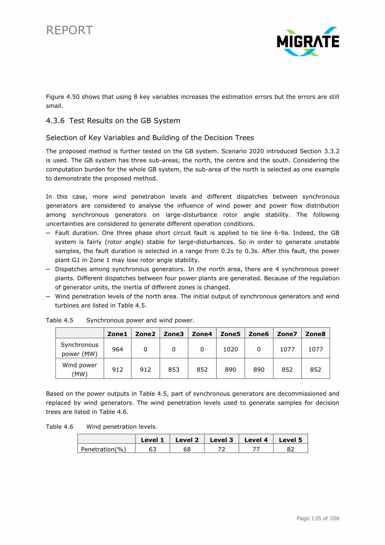
REPORT
Page 135 of 206
Figure 4.50 shows that using 8 key variables increases the estimation errors but the errors are still
small.
4.3.6 Test Results on the GB System
Selection of Key Variables and Building of the Decision Trees
The proposed method is further tested on the GB system. Scenario 2020 introduced Section 3.3.2
is used. The GB system has three sub-areas, the north, the centre and the south. Considering the
computation burden for the whole GB system, the sub-area of the north is selected as one example
to demonstrate the proposed method.
In this case, more wind penetration levels and different dispatches between synchronous
generators are considered to analyse the influence of wind power and power flow distribution
among synchronous generators on large-disturbance rotor angle stability. The following
uncertainties are considered to generate different operation conditions.
─ Fault duration. One three phase short circuit fault is applied to tie line 6-9a. Indeed, the GB
system is fairly (rotor angle) stable for large-disturbances. So in order to generate unstable
samples, the fault duration is selected in a range from 0.2s to 0.3s. After this fault, the power
plant G1 in Zone 1 may lose rotor angle stability.
─ Dispatches among synchronous generators. In the north area, there are 4 synchronous power
plants. Different dispatches between four power plants are generated. Because of the regulation
of generator units, the inertia of different zones is changed.
─ Wind penetration levels of the north area. The initial output of synchronous generators and wind
turbines are listed in Table 4.5.
Table 4.5 Synchronous power and wind power.
Zone1 Zone2 Zone3 Zone4 Zone5 Zone6 Zone7 Zone8
Synchronous
power (MW) 964 0 0 0 1020 0 1077 1077
Wind power
(MW) 912 912 853 852 890 890 852 852
Based on the power outputs in Table 4.5, part of synchronous generators are decommissioned and
replaced by wind generators. The wind penetration levels used to generate samples for decision
trees are listed in Table 4.6.
Table 4.6 Wind penetration levels.
Level 1 Level 2 Level 3 Level 4 Level 5
Penetration(%) 63 68 72 77 82

REPORT
Page 136 of 206
In total, 633 samples are collected, which include 97 dispatches. For each samples, the following
states are recorded as the candidates for key variables.
Table 4.7 Recorded variables in the north area.
Component States
G1,G5,G7,G8 Terminal voltage
Current injected to the grid
Active power & reactive power
Speed, angle, accelerating speed &
inertia
Buses GT1, GT5, GT7, GT8 Voltage magnitude & angle
25 Transmission lines in
the north
Active power
Reactive power
98 variables are selected. These variables represent the post-fault power flow and the generator
status. The bus voltages and transmission line powers define the post–fault power flow. The
terminal voltage, current, and power of generators are related to the electrical torque, which is
influenced by the electrical distance between the generator and the fault. The inertia is one
important factor which influences the post-fault rotor accelerating speed. The speed, angle, and
accelerating speed describe the rotor motion.
The parameters of the decision trees are defined as in Table 4.8. Totally, 100 trees are built to
form a random forest. For each tree, one leaf node only includes one sample. Each variable can be
selected as a property to split a group of samples. Therefore, 98 attributes are used.
Table 4.8 Decision tree parameters.
Tree number Leaf size Attribute number
100 1 98
An initial weight factor, 0.5, is given to each variable. The upper bound of the weight factor is 1,
and the lower bound is 0. The convergence of the optimisation process to find the optimal weight
factors after 1000 iterations is depicted in Figure 4.51. It takes nearly 72 hours to converge on a
computer with Intel I5-2400 and 4G RAM. But it is worth mentioning that this is one-shoot offline
optimisation (i.e. a single run of MVMO – cf. Figure 4.42) and by using only one core of the
computer. Once obtaining the sequence of weight factors, the users need not repeat the
optimisation.

REPORT
Page 137 of 206
Figure 4.51 Errors of decision trees. Scenario 2020 of GB system.
The error is reduced almost 50% after 1000 iterations. Corresponding to the minimum error, the
first 10 variables with the largest weight factors are listed in Table 4.9.
Table 4.9 Selected key variables. Scenario 2020 of GB system.
Number Weight factor State
1 0.98 GT1 bus voltage magnitude
2 0.96 Line 4-5a reactive power
3 0.94 GT1 current magnitude
4 0.91 GT7 voltage magnitude
5 0.87 G1 speed
6 0.85 Line 6-9a active power
7 0.82 Line1-3a active power
8 0.81 Line4-6b active power
9 0.8 GT8 active power
10 0.79 Line2-4b reactive power
11 0.76 GT5 reactive power
From Table 4.9, it can be seen that large-disturbance rotor angle stability is influenced by:
─ The loading level of generator 1, namely the voltage (variable 1) and the current (variable 3).
These two variables determine the active power output of generator 1.
─ The kinetic energy of generator 1, namely the speed (variable 5). The variable represents the
accelerating energy obtained by generator 1 during the fault. In practice, it can be
approximately represented by the terminal bus frequency.
─ The reactive power distribution after the fault, namely the 2nd, 4th, 10th and 11th variables. It is
verified that after the fault, the terminal voltage of generator 1 reduces so that generator 1
cannot output the active power normally. There is not enough reactive power support, so the

REPORT
Page 138 of 206
reactive power flows from other zones to Zone 1. These 4 variables influence the flow of
reactive power to Zone 1.
─ The active power sent out from the north area, namely, the 6th, 7th, 8th, and 9th variables. The
fault prevents the active power transfer from the north area to the centre area, which causes
the generators in Zone 1 to accelerate. Therefore the quantity of active power output will
influence the severity of the fault, and further influence large-disturbance rotor angle stability.
Next, decision trees are built using the above 11 key variables, and are tested under different
operation scenarios. The obtained results are compared against the results obtained using all 98
variables to show that the proposed method can efficiently select key variables for large-
disturbance rotor angle stability assessment.
Test Results
65% wind Penetration
60 tests are made for this penetration level. From Figure 4.52, it can be seen that the estimation
done by using 11 key variables also provides similar accuracy as the estimation done by using 98
variables.
Figure 4.52 (left) Results with 98 variables; (right) Results with 11 key variables. O = Estimation;
X = Simulation.
Another point noticed here is that there are some points with relatively large estimation errors.
This is caused by the sudden transition from rotor angle stability to rotor angle instability due to a
minor change of fault duration, which is shown in Figure 4.53 and Figure 4.54. Indeed, GB system
is fairly stable for large disturbances. Therefore, in order to generate unstable samples, the fault
duration is increased from 0.2s to 0.3s. With the increasing of fault duration, GB system becomes
more prone to instability. For example, in the border between rotor angle stability and instability, if
the fault duration is slightly changed from 0.271s to 0.272s, the difference of one millisecond
causes rotor angle instability (please see Figure 4.54). On the edge to instability, usually the
artificial intelligence based methods have relatively large errors.

REPORT
Page 139 of 206
Figure 4.53 G1 angle with a fault duration of 0.271 s.
Figure 4.54 G1 angle with a fault duration of 0.272 s.
The case in Figure 4.54 is unstable. This figure shows a first swing instability. It is worth clarifying
that when the angle exceeds 180 degrees, PowerFactory restarts the angle from -180 degrees.
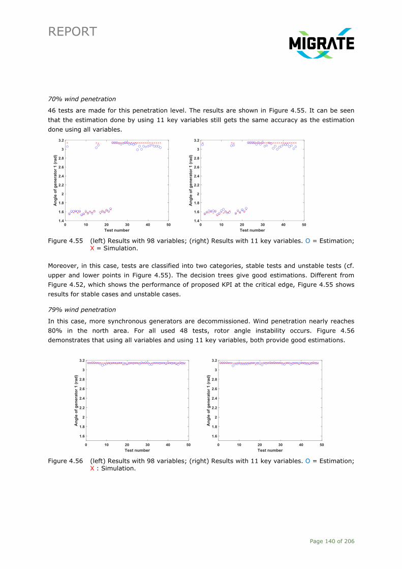
REPORT
Page 140 of 206
70% wind penetration
46 tests are made for this penetration level. The results are shown in Figure 4.55. It can be seen
that the estimation done by using 11 key variables still gets the same accuracy as the estimation
done using all variables.
Figure 4.55 (left) Results with 98 variables; (right) Results with 11 key variables. O = Estimation; X = Simulation.
Moreover, in this case, tests are classified into two categories, stable tests and unstable tests (cf.
upper and lower points in Figure 4.55). The decision trees give good estimations. Different from
Figure 4.52, which shows the performance of proposed KPI at the critical edge, Figure 4.55 shows
results for stable cases and unstable cases.
79% wind penetration
In this case, more synchronous generators are decommissioned. Wind penetration nearly reaches
80% in the north area. For all used 48 tests, rotor angle instability occurs. Figure 4.56
demonstrates that using all variables and using 11 key variables, both provide good estimations.
Figure 4.56 (left) Results with 98 variables; (right) Results with 11 key variables. O = Estimation; X : Simulation.

REPORT
Page 141 of 206
4.3.7 Conclusions and Recommendations
This section presented the KPI developed for the assessment of large-disturbance rotor angle
stability. The two most important innovations of this work are:
─ The accuracy of decision trees is used to select key variables to estimate the maximum angular
deviation. Taking key variables as the inputs of decision trees entails a good accuracy.
─ The selection of key variables and the optimisation of decision trees are made at the same time
via a weight factor. The weight factor is optimised by MVMO.
The presented results on 9 bus system and GB system show that the proposed method is efficient
and feasible. It selects correctly a few of key variables for decision trees, and at the same time
keeps a good estimation accuracy for large-disturbance rotor angle stability. It is noted that on the
edge to instability, decision trees may have some relatively large errors. This is a common
challenge for all artificial intelligence based methods. More research effort should be put into
solving the misjudgement on the border between stability and instability.
Before using this method in real power systems, adequate tests are necessary. To ensure a
satisfactory performance, a minimum number of samples of possible system operating conditions
and disturbances are needed for training the decision trees. This is a general requirement for
artificial intelligence based methods. That is to say, if artificial intelligence based methods do not
obtain enough good knowledge from the samples, they could probably fail to give correct
estimations. A simple approach can be used to define the minimum number of samples: select a
set of few critical faults. The possible faults in real systems are numerous, but not every fault
causes transient instability. Therefore, the faults which never cause large-disturbance rotor angle
instability as well as the faults which always (in any operating condition) cause large-disturbance
rotor angle instability can be neglected for decision trees. The focus can be put on faults which do
not cause large-disturbance rotor angle instability in normal operation conditions, but may cause
large-disturbance rotor angle instability in stressed operation conditions. Such approach was
illustrated in this report.
On the other hand, any independent test should be made by using values of the system variables
which are in the range of collected samples. That is to say, if a complete new and different
operation condition, which has radically different characteristics with respect to the considered
samples, is tested, maybe decision trees obtained by the proposed method cannot give a good
estimation. Two possible solutions can be taken to improve the performance: enrich the used
sample database, namely, providing more knowledge to decision trees to make them smarter, or
adding self-learning skills to decision trees.
Once decision trees meet the requirement of system operators with respect to acceptable accuracy,
they can be used for large-disturbance rotor angle stability monitoring and control. One possible
implementation is shown in Figure 4.57. First, with the help of off-line training (cf. Figure 4.42),
different groups of decision trees are obtained for different faults. In practice, when a fault occurs,
Disturbance indicator will send the fault information to a classifier. This classifier will select the

REPORT
Page 142 of 206
corresponding group of decision trees, like group 1, group 2. PMU measurements are also sent to
the selected group of decision trees. Decision trees will output the large disturbance rotor angle
stability indicator, like Margin 1, Margin 2, etc.
Disturbance indicator -
IED
.
.
.
Group 1
Group 2
Group n
Margin 1
Margin 2
Margin n
Classifier of
Decision trees
PMU measurement
Off-line
decision trees
training
(cf. Fig. 4.41)
Figure 4.57 Proposed implementation for decision trees.
Figure 4.58 gives an example of a possible application. In the example, there are n key variables
and a group of decision trees to estimate the maximum angle difference 𝛿𝑖 − 𝛿𝑗 . The first key
variable is perturbed from K1 to K’1 and other key variables are kept constant. The decision trees
are executed to obtain the resulting increment of angle difference ∆(𝛿𝑖 − 𝛿𝑗). The sensitivity of angle
difference to K1 is defined as:
𝑆K1 =∆(𝛿𝑖 − 𝛿𝑗)
𝐾1′ − 𝐾1
(4.16)
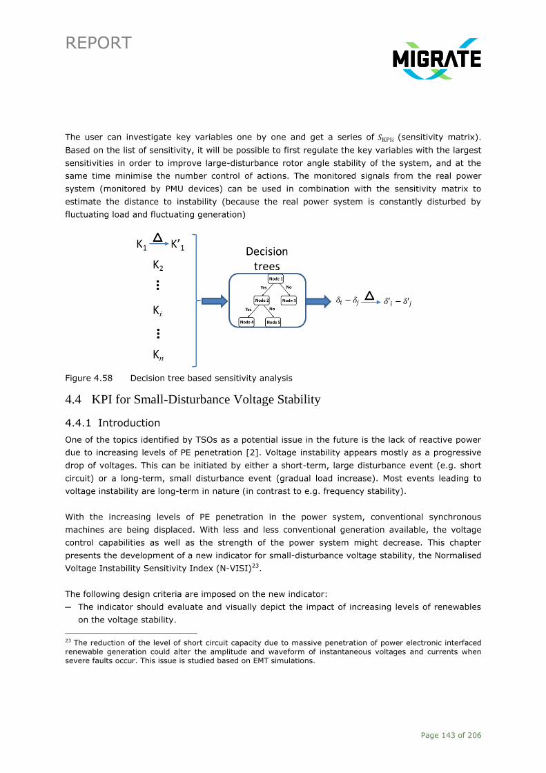
REPORT
Page 143 of 206
The user can investigate key variables one by one and get a series of 𝑆KPI𝑖 (sensitivity matrix).
Based on the list of sensitivity, it will be possible to first regulate the key variables with the largest
sensitivities in order to improve large-disturbance rotor angle stability of the system, and at the
same time minimise the number control of actions. The monitored signals from the real power
system (monitored by PMU devices) can be used in combination with the sensitivity matrix to
estimate the distance to instability (because the real power system is constantly disturbed by
fluctuating load and fluctuating generation)
Figure 4.58 Decision tree based sensitivity analysis
4.4 KPI for Small-Disturbance Voltage Stability
4.4.1 Introduction
One of the topics identified by TSOs as a potential issue in the future is the lack of reactive power
due to increasing levels of PE penetration [2]. Voltage instability appears mostly as a progressive
drop of voltages. This can be initiated by either a short-term, large disturbance event (e.g. short
circuit) or a long-term, small disturbance event (gradual load increase). Most events leading to
voltage instability are long-term in nature (in contrast to e.g. frequency stability).
With the increasing levels of PE penetration in the power system, conventional synchronous
machines are being displaced. With less and less conventional generation available, the voltage
control capabilities as well as the strength of the power system might decrease. This chapter
presents the development of a new indicator for small-disturbance voltage stability, the Normalised
Voltage Instability Sensitivity Index (N-VISI)23.
The following design criteria are imposed on the new indicator:
─ The indicator should evaluate and visually depict the impact of increasing levels of renewables
on the voltage stability.
23 The reduction of the level of short circuit capacity due to massive penetration of power electronic interfaced renewable generation could alter the amplitude and waveform of instantaneous voltages and currents when severe faults occur. This issue is studied based on EMT simulations.

REPORT
Page 144 of 206
─ The indicator or its calculation process should preferably identify weak nodes in the system in
order to carry out further analysis on specific buses.
─ The indicator should give insight in the distance to instability.
─ The indicator should be relatively easy implementable for control room applications.
For the long-term voltage stability assessment, it is assumed that the wind turbines have a fixed
active power output.
4.4.2 Definitions
Power Electronics-Interfaced Generation (PEIG) is defined here as infeed that is connected to the
grid using PE. This can be generation and import through HVDC. Power Electronics-Interfaced
Device (PEID) is defined here as any device that is connected to the grid using PE. This can be
generation, loads, HVDC converters, etc.
System Non-Synchronous Penetration (SNSP)
The System Non-Synchronous Penetration (SNSP), as defined in [100] is an indication of the ratio
of PEIG over the system load and HVDC export and is defined as:
where:
Pwind = the wind generation in the system (MW)
PHVDC(import) = the import through HVDC interconnections (MW)
Pload = the system demand (MW)
PHVDC(export) = the export through HVDC interconnections (MW)
Whereas this indicator is a useful one in terms of expressing the relative PEIG in a system, the
results presented in [100] illustrate values of SNSPs larger than 100%. Based on the above
formula this means that the sum of wind generation and HVDC imports is larger than the sum of
the demand and HVDC exports.
As this is not possible in a balanced power system, a modified SNSP index (SNSP*) is derived to
indicate the level of PEIG in a system. The aim is to derive a mathematical expression for the
SNSP* where SNSP* is defined as the ratio of the PE infeed (i.e. PEIG) over the total system
demand. It is assumed that the power system is balanced at all times, i.e. the total generation
(synchronous as well as non-synchronous) is equal to the total demand, ergo SNSP* is defined as:
SNSP = 𝑃𝑤𝑖𝑛𝑑 + 𝑃𝐻𝑉𝐷𝐶(𝑖𝑚𝑝𝑜𝑟𝑡)
𝑃𝑙𝑜𝑎𝑑 + 𝑃𝐻𝑉𝐷𝐶(𝑒𝑥𝑝𝑜𝑟𝑡) (4.17)
𝑆𝑁𝑆𝑃∗ =𝑃𝐸𝐼𝐺
𝑃𝑙𝑜𝑎𝑑=
𝑃𝐸𝐼𝐺
𝑃𝐸𝐼𝐺 + 𝐶𝑜𝑛𝑣𝑒𝑛𝑡𝑖𝑜𝑛𝑎𝑙 𝐺𝑒𝑛𝑒𝑟𝑎𝑡𝑖𝑜𝑛
(4.18)

REPORT
Page 145 of 206
Whereas equations (4.17) and (4.18) are in essence the same, the definition in equation (4.18) is
helpful in deriving step by step equation (4.24).
In terms of energy exchanges (imports and exports), a power system can conceptually have 5
possible independent operating states: no exchanges (case 1), AC export (case 2), AC import
(case 3), DC export (case 4), and DC import (case 5). In case 1, SNSP* is therefore defined as:
In case 2, there is an AC export out of the system, which acts as an extra load on the system.
Assuming fixed Pwind and Pload this means that conventional generation will increase to cover this
extra demand. SNSP* is now defined as:
When there is an AC import (case 3) and fixed Pwind and Pload the conventional generation decreases
by the amount of the AC import. SNSP* is then defined as:
In the case of a DC export and fixed Pwind and Pload (case 4), the conventional generation will
increase again in order to cover the extra demand. The increase in the output of the conventional
generation is equal to the value of the DC export. SNSP* is now defined as:
In the last case, the system has a DC import (case 5). Again Pwind and Pload are assumed fixed. The
DC import is categorised as PEIG and therefore the SNSP* is now defined as:
An example of all these 5 cases is given in Figure 4.59.
𝑆𝑁𝑆𝑃∗ =𝑃𝑤𝑖𝑛𝑑
𝑃𝑙𝑜𝑎𝑑 − 𝑃𝑤𝑖𝑛𝑑
(4.19)
𝑆𝑁𝑆𝑃∗ =𝑃𝑤𝑖𝑛𝑑
𝑃𝑙𝑜𝑎𝑑 − 𝑃𝑤𝑖𝑛𝑑 + 𝐴𝐶𝑒𝑥𝑝𝑜𝑟𝑡 (4.20)
𝑆𝑁𝑆𝑃∗ =𝑃𝑤𝑖𝑛𝑑
𝑃𝑙𝑜𝑎𝑑 − 𝑃𝑤𝑖𝑛𝑑 − 𝐴𝐶𝑖𝑚𝑝𝑜𝑟𝑡 (4.21)
𝑆𝑁𝑆𝑃∗ =𝑃𝑤𝑖𝑛𝑑
𝑃𝑙𝑜𝑎𝑑 − 𝑃𝑤𝑖𝑛𝑑 + 𝐷𝐶𝑒𝑥𝑝𝑜𝑟𝑡 (4.22)
𝑆𝑁𝑆𝑃∗ =𝑃𝑤𝑖𝑛𝑑 + 𝐷𝐶𝑖𝑚𝑝𝑜𝑟𝑡
𝑃𝑙𝑜𝑎𝑑 − 𝑃𝑤𝑖𝑛𝑑 + 𝐷𝐶𝑒𝑥𝑝𝑜𝑟𝑡 (4.23)

REPORT
Page 146 of 206
Figure 4.59 SNSP* Example.
Combining the above cases would yield the following generic mathematical definition for SNSP*:
Another simple index ‘PE to load’ ratio (PE2L) is proposed and is defined as the part of the load (i.e.
the demand in the system excluding AC imports, AC exports, and DC exports) that is covered by
PEIG. The mathematical expression for PE2L is:
where:
∑Pwind = the total wind generation
∑PDC,import = the total imports from HVDC interconnections
Pload,system = the load of the system (excluding exports and AC imports)
The goal of this indicator is to get insight in which part of the load is supplied by PEIG. In contrast
to the SNSP* this indicator can be larger than 1, as exports are excluded. A value larger than 1
implies the infeed from PEIG is larger than the load and that the remaining energy is exported.
CASE 1Pwind = 500 MWLoad = 1000 MW
CASE 2Pwind = 500 MWLoad = 1000 MW
CASE 3Pwind = 500 MWLoad = 1000 MW
CASE 4Pwind = 500 MWLoad = 1000 MW
CASE 5Pwind = 500 MWLoad = 1000 MW
AC export = 250 MW
AC import = 250 MW
DC export = 250 MW
DC import = 250 MW
PEID = 500 + 0 = 500Conv. Gen. = 1000 – 500 = 500
𝑆𝑁𝑆𝑃∗ = 500
500+ 500= 0.5
PEID = 500 + 0 = 500Conv. Gen. = 1000 – 500 + 250 = 750
𝑆𝑁𝑆𝑃∗ = 500
500+ 50= 0.
PEID = 500 + 0 = 500Conv. Gen. = 1000 – 500 - 250 = 250
𝑆𝑁𝑆𝑃∗ = 500
500+ 250= 0.6
PEID = 500 + 0 = 500Conv. Gen. = 1000 – 500 + 250 = 750
𝑆𝑁𝑆𝑃∗ = 500
500+ 50= 0.
PEID = 500 + 250 = 750Conv. Gen. = 1000 – 500 - 250 = 250
𝑆𝑁𝑆𝑃∗ = 500+ 250
500+ 250+ 250= 0. 5
𝑆𝑁𝑆𝑃∗ =∑𝑃𝑤𝑖𝑛𝑑 + ∑𝑃𝐷𝐶,𝑖𝑚𝑝𝑜𝑟𝑡
𝑃𝑙𝑜𝑎𝑑,𝑠𝑦𝑠𝑡𝑒𝑚 + ∑𝑃𝐴𝐶,𝑒𝑥𝑝𝑜𝑟𝑡 + ∑𝑃𝐷𝐶,𝑒𝑥𝑝𝑜𝑟𝑡 − ∑𝑃𝐴𝐶,𝑖𝑚𝑝𝑜𝑟𝑡
(4.24)
𝑃𝐸2𝐿 = ∑𝑃𝑤𝑖𝑛𝑑 + ∑𝑃𝐷𝐶,𝑖𝑚𝑝𝑜𝑟𝑡
𝑃𝑙𝑜𝑎𝑑,𝑠𝑦𝑠𝑡𝑒𝑚
(4.25)

REPORT
Page 147 of 206
A comparison between the modified SNSP (SNSP*), the original SNSP, and the PE2L index is given
in Table 4.10. The difference in the indices, arising for case 2 and case 3, can be explained by the
fact that the definition for SNSP does not contain the AC exchanges.
Table 4.10 SNSP Comparison.
Case SNSP* PE2L SNSP
Case 1 0.5 0.5 0.5
Case 2 0.4 0.5 0.5
Case 3 0.67 0.5 0.5
Case 4 0.4 0.5 0.4
Case 5 0.75 0.75 0.75
V/V0
The V/V0 index [101], [102], is a rather simple index that determines the weakest bus in a power
system. It is the ratio between the actual bus voltage V and a reference voltage V0. The actual bus
voltage V is known from power flow studies (offline) or state estimation (online). V0 is the voltage
at the same bus but with all loads set to 0. This voltage is obtained using power flow simulations.
The ratio V/V0 gives the voltage stability index. The value can be between 1 and 0 and the lower
the index, the weaker that specific bus is.
The V/V0 indices across the buses create a voltage stability map of the power system, allowing for
immediate detection of weak nodes. Detection of weak areas in the system is beneficial and even
more for larger systems. Another advantage of this index is that it has practically no computational
burden on the system, and can therefore be carried out more frequently (e.g. for load increases,
redispatch, topology changes, etc.). This index has been used for online voltage stability
monitoring (identification of weak buses) since 1995 [103].
The results from the V/V0 analysis have been validated using Short Circuit Capacity (SCC)
calculations for the generic test case. In more than 80% of the simulated cases, the V/V0 method
correctly identified the 3 worst buses of the system (compared with the results from the SCC
calculations).
PV Curve
The Power-Voltage characteristic at buses, also known as PV curves, is a popular method especially
in the industry for determining the small-disturbance voltage stability of power systems [104]. The
mathematical formulation for the PV curve is derived as follows. Assume the 2 bus system as given
in Figure 4.60.

REPORT
Page 148 of 206
Figure 4.60 Test model for voltage stability.
VS is the sending end voltage and has a phase displacement 𝜑1 compared to a reference signal:
VS=𝑉𝑆∠𝜑1 . VR is the receiving end voltage and has a phase displacement 𝜑2 : VR=𝑉𝑅∠𝜑2 . The
transmission line has a complex impedance Z, consisting of a resistance R and reactance X. Also,
the following relationships exist:
Let 𝜑2 − 𝜑1 = 𝜃 be the load angle 𝑆 =𝑉𝑅𝑉𝑆𝑒
−𝑗(𝜃−𝜓)
𝑍−
𝑉𝑅2𝑒𝑗𝜓
𝑍
Also: 𝑒−𝑗𝜃 = 𝑐𝑜𝑠𝜃 − 𝑗𝑠𝑖𝑛𝜃 and 𝑒𝑗𝜃 = 𝑐𝑜𝑠𝜃 + 𝑗𝑠𝑖𝑛𝜃 therefore:
AC
R + jX
BUS 1 BUS 2S = P + jQ
VS VR
𝑍 = 𝑅 + 𝑗𝑋 = 𝑍𝑒𝑗𝜓 (4.26)
𝑉𝑆 = 𝑉𝑆𝑒−𝑗𝜑1 (4.27)
𝑉𝑅 = 𝑉𝑅𝑒−𝑗𝜑2 (4.28)
𝐼 = 𝑉𝑆 − 𝑉𝑅
𝑍
(4.29)
𝑆 = 𝑉𝑅𝐼∗ ⇒ 𝑆 = 𝑆 = 𝑉𝑅 (
𝑉𝑆 − 𝑉𝑅
𝑅 + 𝑗𝑋)
∗
(4.30)
𝑆 = 𝑉𝑅𝑒−𝑗𝜑2 (
𝑉𝑆𝑒𝑗𝜑1 − 𝑉𝑅𝑒
𝑗𝜑2
𝑍𝑒−𝑗𝜓) (4.31)
𝑆 =𝑉𝑅𝑉𝑆𝑍
(cos (𝜃 − 𝜓) − 𝑗𝑠𝑖𝑛(𝜃 − 𝜓)) −𝑉𝑅
2
𝑍(𝑐𝑜𝑠𝜓 + 𝑗𝑠𝑖𝑛𝜓)
(4.32)
𝑆 =𝑉𝑅𝑉𝑆𝑍
cos(𝜃 − 𝜓) − 𝑗𝑉𝑅𝑉𝑆𝑍
𝑠𝑖𝑛(𝜃 − 𝜓) −𝑉𝑅
2
𝑍𝑐𝑜𝑠𝜓 − 𝑗
𝑉𝑅2
𝑍𝑠𝑖𝑛𝜓)
(4.33)
𝑆 =𝑉𝑅𝑉𝑆𝑍
cos(𝜃 − 𝜓) −𝑉𝑅
2
𝑍𝑐𝑜𝑠𝜓 + 𝑗 (
−𝑉𝑅𝑉𝑆𝑍
𝑠𝑖𝑛(𝜃 − 𝜓) −𝑉𝑅
2
𝑍𝑠𝑖𝑛𝜓) (4.34)
𝑃 = 𝑅𝑒(𝑆) =𝑉𝑅𝑉𝑆𝑍
cos(𝜃 − 𝜓) −𝑉𝑅
2
𝑍𝑐𝑜𝑠𝜓 ⇒
𝑐𝑜𝑠𝜓
𝑍𝑉𝑅
2 −𝑉𝑆 cos(𝜃 − 𝜓)
𝑍𝑉𝑅 + 𝑃 = 0
(4.35)

REPORT
Page 149 of 206
For the active power equation, which is a second order equation for VR, the sending end voltage,
the load angle, and the line impedance can be assumed constant. Solving the equation for the
receiving end voltage, the influence of increasing active power transfers P on the receiving end
voltage VR can be investigated. When this is plotted for several values of P, the PV curve is
obtained.
The major strengths of the PV curve are its robustness, computational efficiency, and easy
implementation as a control room application. The shortcomings are in the fact that the PV curve
assumes a constant load angle (with increasing loads) as explained above. It also does not directly
give information on the ‘speed’ to instability, especially with increasing levels of PE2L.
The KPI that is proposed in this chapter aims at keeping the strengths of the PV curve while
addressing the shortcomings. The proposed procedure will also identify the weak buses in a system,
so that these buses can be targeted for further analysis.
4.4.3 Proposed Indicator: Calculation Procedure
The Normalised Voltage Instability Sensitivity Index (N-VISI) is proposed as a new indicator for
assessing small-disturbance voltage stability. The flowchart in Figure 4.61 illustrates the required
steps to populate the data for the calculation of the N-VISI. As a first step the V/V0 analysis and
SCC calculations are carried out (please refer to Section 4.4.2 for more the details on the V/V0
index). The V/V0 index gives the weakest bus (or set of weakest buses) in the power system. For
this identified bus, a set of power flows is solved while increasing the load uniformly across the
system until divergence of the power flow solution occurs. For every power flow solution, the
changes in voltage and load are recorded for manual data processing. These steps are repeated for
a defined set of weak buses. These steps are automated using python.
Figure 4.62 illustrates the steps for the manual data processing. The N-VISI itself is the result of
the manual data processing steps. Once the loads and corresponding voltages are recorded for the
set of weak buses, curve fitting is applied to obtain a mathematical function of the P-V relationship.
As shown in the previous section, this relationship is non-linear. Therefore, polynomial regression
has been used for curve fitting. The first derivative of the polynomial is then calculated and
represents the ‘speed’ towards the nose point (instability point). For each of the load levels defined
in the previous step, the derivative (i.e. the sensitivity) is calculated. As these sensitivities have a
wide range for different cases, they are normalised for comparison purposes. Therefore the index
N-VISI can have a value between 0 and 1: the higher the index, the faster the nose point is
reached, ergo the less stable the system becomes24.
24 It should be mentioned that the effect of variations in tap position of transformers or compensation devices on the N-VISI is not explicitly taken in into account. However, as these variations alter the operating condition, the N-VISI can be easily calculated for these operating conditions as well.
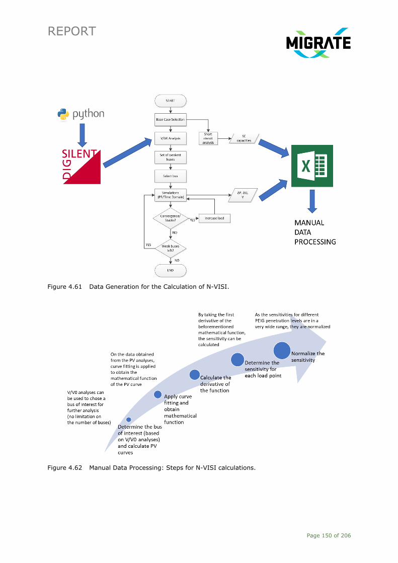
REPORT
Page 150 of 206
Figure 4.61 Data Generation for the Calculation of N-VISI.
Figure 4.62 Manual Data Processing: Steps for N-VISI calculations.

REPORT
Page 151 of 206
4.4.4 Results for Generic Test Case 2
The processes described in the previous section have been implemented for generic test case 2.
For voltage stability, this is the IEEE 9 bus system in which certain modifications are done (for
more details, see Section 3.2.4).
As a first step, the V/V0 and SCC analyses were done. The results are presented for 3 cases in
Figure 4.63. The Base Case represents a conventional power system with no PEIG. The Increased
PE case is a representation of a RES-dominated power system with a PE2L ratio of approximately
70%. In this case the wind generation displaces the conventional generator G2 at bus 2. In the
Reduced SG (reduced synchronous generation) case the conventional generator G2 at bus 2 is
disconnected again. No wind generation is connected to the grid at this moment, i.e. the power
balance is maintained by increased production of the remaining conventional generators.
Figure 4.63 Results of V/V0 and SCC Analyses for Generic Test Case.
Compared to the Base Case, one can observe that in the Increased PE case the V/V0 index
decreases for several buses. The largest relative decrease can be observed for bus 2 and bus 7.
This can be explained by the fact that bus 2 contains generator G2, which is switched off in the
Increased PE case. A step up transformer connects G2 to bus 7, which therefore is also directly
influenced by the state of G2. Buses 5, 6 and 8 are load buses.
Bus 5 has the lowest V/V0 index and is therefore the weakest bus. This bus has the largest active
and reactive power load. When switching off G2, the reactive power has to be provided by the
remaining conventional generators. The increased reactive power transfer leads to lower voltages

REPORT
Page 152 of 206
in this case. As bus 6 is located between G1 and G3, the absence of G2 is not affecting the bus
voltage.
The short circuit analysis carried out on the three cases reveals that the Reduced SG case has the
lowest short circuit capacity. Although G2 is also switched off in the Increased PE case, the WTs in
this case deliver a small amount of short circuit current, resulting in an overall higher short circuit
capacity compared to the Reduced SG case.
Both methods, the V/V0 as well as the SCC, identify buses 5, 6, and 8 as the weakest buses (bus 2
and 7 are not considered because of the switching off of the conventional generator).
For bus 5 the SCC is given for different PE2L ratios in Figure 4.64. In the same figure the
development of the critical load with increasing levels of PE2L is illustrated. The critical load is
defined as the maximum load that can be accommodated by the system while maintaining
acceptable voltage levels at all buses. Increasing the load even further would result in a voltage
collapse. Generators G2 and G3 are modelled as 10 parallel machines. With increasing levels of
PEIG, the number of parallel machines is reduced, starting with generator G2.
Figure 4.64 Critical P and SCC vs PE2L ratio.
The general trend is a decreasing one: the critical load as well as the SCC decrease with increasing
PE2L ratios. Increasing PE2L ratios displaces conventional generation. This reduces the long-term
voltage support available from conventional generation. Also, as conventional generators have
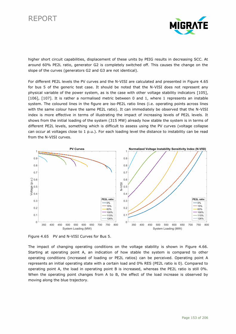
REPORT
Page 153 of 206
higher short circuit capabilities, displacement of these units by PEIG results in decreasing SCC. At
around 60% PE2L ratio, generator G2 is completely switched off. This causes the change on the
slope of the curves (generators G2 and G3 are not identical).
For different PE2L levels the PV curves and the N-VISI are calculated and presented in Figure 4.65
for bus 5 of the generic test case. It should be noted that the N-VISI does not represent any
physical variable of the power system, as is the case with other voltage stability indicators [105],
[106], [107]. It is rather a normalised metric between 0 and 1, where 1 represents an instable
system. The coloured lines in the figure are iso-PE2L ratio lines (i.e. operating points across lines
with the same colour have the same PE2L ratio). It can immediately be observed that the N-VISI
index is more effective in terms of illustrating the impact of increasing levels of PE2L levels. It
shows from the initial loading of the system (315 MW) already how stable the system is in terms of
different PE2L levels, something which is difficult to assess using the PV curves (voltage collapse
can occur at voltages close to 1 p.u.). For each loading level the distance to instability can be read
from the N-VISI curves.
Figure 4.65 PV and N-VISI Curves for Bus 5.
The impact of changing operating conditions on the voltage stability is shown in Figure 4.66.
Starting at operating point A, an indication of how stable the system is compared to other
operating conditions (increased of loading or PE2L ratios) can be perceived. Operating point A
represents an initial operating state with a certain load and 0% RES (PE2L ratio is 0). Compared to
operating point A, the load in operating point B is increased, whereas the PE2L ratio is still 0%.
When the operating point changes from A to B, the effect of the load increase is observed by
moving along the blue trajectory.

REPORT
Page 154 of 206
The load in operating point C is identical to operating point A; the PE2L ratio now is 100%. When
the operating point changes from A to C, this symbolises an increase in the PE2L ratio. The effect
of this change on the voltage stability is observed by moving from the blue line to the purple line.
In operating point D the load as well as the PE2L ratio is changed.
Figure 4.66 N-VISI Curves for Bus 5.
As can be seen from the results of the N-VISI this new indicator not only gives insight into the
distance to instability, but also illustrates effectively the impact of system changes (PE2L ratio and
load) on the voltage stability. As the N-VISI uses the complete set of data of each PV curve, the
faster decrease of e.g. the yellow line (63% PE2L ratio), and the earlier collapse of the purple line
(100% PE2L ratio) are also taken into account in the respective N-VISI. That is why the N-VISI for
the 100% PE2L ratio is higher from the initial loading already.
4.4.5 Validation on the GB Power System
The same processes as defined in the previous sections are implemented in the GB system. Based
on the V/V0 results, the results for bus 15 are presented in Figure 4.67. In this figure, scenario
GG2020 is used as a starting point. The N-VISI analysis is carried out on this case. As a next step,
the PE2L ratio is increased to 40% and afterwards to 50%. It can be observed that for the 40%
case the voltage stability is improved. This has to do with the dispatch: wind generation is
increased in the near vicinity, leading to an increased margin for reactive power control of
conventional generation. In the 45% case the changes in the network are done electrically far from
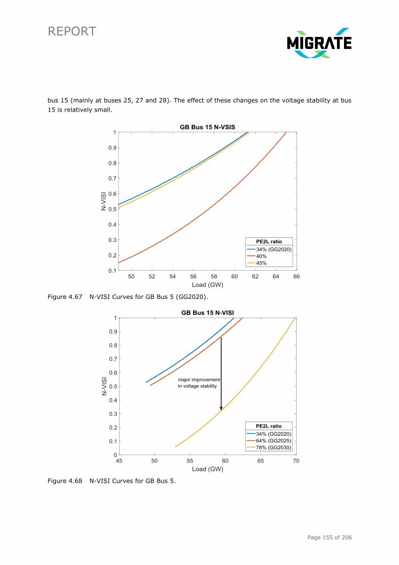
REPORT
Page 155 of 206
bus 15 (mainly at buses 25, 27 and 28). The effect of these changes on the voltage stability at bus
15 is relatively small.
Figure 4.67 N-VISI Curves for GB Bus 5 (GG2020).
Figure 4.68 N-VISI Curves for GB Bus 5.

REPORT
Page 156 of 206
The N-VISI curves for bus 15 are shown in Figure 4.68. It should be mentioned that whereas in the
previous results the PE2L ratio was increased on the same network, the results shown in Figure
4.68 are based on 3 different cases of the Gone Green scenarios. The years 2020, 2025, and 2030
of the Gone Green scenarios are analysed. Based on the previous results, one would expect the
voltage stability to deteriorate with increasing levels of PE2L.
There are 2 reasons why the opposite is happening here:
1. When looking at the generation at node 15, it is observed that 1 GW of wind farms is connected
at this node for the scenario GG2030. The increased wind generation results in decreased
output of the conventional generators, which results in an increased margin for reactive power
control. Therefore more load can be accommodated. This is reflected in N-VISI curve.
2. The number of conventional generation at node 15 is increased in the GG2030 scenario. The
effect is the same: the margin for reactive power control from conventional generation is
increased, resulting in a more stable system.
These results show what is confirmed in [103] as well: indicators based on sensitivities change
more dynamically if changes occur electrically close to the bus under investigation. When changes
such as load increase or even the dispatch changes at a bus that is electrically far from the bus
under investigation, the effect is rather small. This confirms the rather local impact of voltage
stability, in contrast to frequency stability.
As proven here with the analysis, this index can also be used for investigation and understanding
how the voltage stability changes for different planning scenarios (GG2020 scenario versus
GG2030 scenario).
4.4.6 Conclusions and Recommendations
The aim of this chapter was to develop a new KPI for voltage stability. The Normalised Voltage
Instability Sensitivity Index (N-VISI) is developed and proposed. This index has the following
advantages:
─ It gives information on the distance to instability in terms of sensitivities.
─ The influence of changes in the system (PE2L ratios and load) on the voltage stability can be
illustrated in a comprehensive manner.
─ The process for calculating the N-VISI defines the weak buses in the system by using the V/V0
analysis.
─ Using the V/V0 method for each iteration can show how the weak buses in the power system
shift as a result of specific actions.
─ It has been shown that the index is also useful in analysing and understanding how voltage
stability changes for different planning scenarios (GG2020 vs GG2030).
The following disadvantages have been observed with the N-VISI:

REPORT
Page 157 of 206
─ The load increase is modelled based on a uniform load increase across all the load buses. A new
operating point based on an asymmetrical load increase would require carrying out new
analyses.
─ The index is situation specific. Changes in the network topology, dispatch or loading will require
new calculations.
However, because the required calculations are based on steady state simulations and can be
performed fast, this is not seen as a major issue.
Roadmap for Control Room Implementation
The N-VISI index developed in this chapter can be implemented in the control room. For each step
in the calculation process the requirements are presented as follows. The V/V0 analysis requires
two inputs. The actual bus voltages are known in the SCADA. For calculating the V0 voltages, the
actual grid topology is required, which can be retrieved from the SCADA as well. A steady state
power flow program is required to calculate the V0 voltages, after which the V/V0 analysis can be
conducted. Next, a set of weak buses is selected based on the V/V0 indices and for each bus N-
VISI curves are calculated for different levels of PE2L ratios25.
The steady state power flow program can be used to simulate the P-V characteristics at each of the
identified buses and for each of the PE2L ratios. The PE2L ratios can be defined based on the
operational planning schedules (network topology, dispatched generation, exports, and imports)
which are known in advance. In order to calculate the N-VISIs, a software capable of doing the
defined mathematical operations (polynomial regression and derivative calculation) is required.
Once the N-VISIs are calculated, a visualisation tool is needed to illustrate the current operating
point on the iso-PE2L lines of the N-VISI vs Load graphs.
However, for implementing the KPI for real time operations, there are a number of challenges:
1. Determining the PE2L ratio in real time is practically impossible at this moment. The reason for
this is that the transmission system operator can only observe the vertical load (i.e. load at the
transformer between TSO and DSO. Installed RES generation on DSO level is subtracted from
the real, actual demand).
2. As the power system in reality is in quasi steady state, control room engineers need to define
thresholds based on their operational experience (e.g. minimum observed change in load) for
activation of the N-VISI calculations.
Future Work
Voltage stability is local phenomenon. With the replacement of transmission system connected
conventional power plants by transmission- and distribution system connected RES, the distribution
system is changing towards an active distribution network. Active distribution networks can support
25 Whereas the aim of the selection of buses is to concentrate on weak parts of the system, it should be mentioned that the N-VISI can be calculated for all the buses in the system.

REPORT
Page 158 of 206
to a certain extent the secure operation of the power system (including voltage stability) [108].
With decreasing reactive power controllability in the transmission system on the one hand, and
increasing reactive power controllability in the distribution system on the other hand, the impact of
distribution system connected RES should be further investigated. As TSOs have limited knowledge
of the RES availability at distribution level, a strong cooperation between the TSO and DSO will be
required, when harnessing the reactive power support from distribution system connected RES.
This is a topic for further research.
4.5 KPI for Sub-Synchronous Controller Interactions
This section discusses the development of an indicator for determining the ‘distance’ to instability
for controller interactions. The phenomenon of Controller Interactions (CI) has no distance to
instability in the form that exists for the classical power system phenomena. This is a result of the
mechanisms leading to CI, which will be explained in the subsequent subsections. The distance to
CI proposed in this section could theoretically be used to predict the occurrence of CI.
4.5.1 Introduction
The motivation of investigating the current issue is that participants of the TSO questionnaire
(deliverable D1.1 [2]) mentioned ‘PE controller interaction with each other and passive AC
components’ as one of the problems resulting from increasing penetration of PE in the transmission
system. This issue ranked 5th in terms of severity, probability and timeframe.
When analysing this problem, it should be observed that these are technically 2 independent issues.
The first is the interaction of PE controllers with passive AC components. The second is the problem
of controller interactions of PE devices among each other.
In Table 4.11, a classification of the possible interactions between conventional generators, series
capacitors and Power Electronic-Interfaced Devices (PEID) in power systems is shown.
Table 4.11 Classification of Interactions in Power Systems.
Conventional Generator Series Capacitor PEID
Conventional Generator Inter area oscillations SSR SSTI
Series Capacitor SSR
SSCI
PEID SSTI SSCI CCI
The interaction between conventional generators can result in oscillations. Oscillations resulting
from a single generator are called local modes, whereas oscillations associated with groups of
generators are called interarea modes [109]. These interactions involve the mechanical shaft of the
generators and are therefore categorised as electromechanical oscillations.
The interactions between a turbine-generator and a series capacitor (e.g. a series compensated
transmission line) is defined as Sub-Synchronous Resonance (SSR). A resonance is defined as ‘the
enhancement of the response of a physical system to a periodic excitation when the excitation

REPORT
Page 159 of 206
frequency is equal to a natural frequency of the system [110]. The interaction results in either
electrical oscillations (induction generator effect, see [111]) or electromechanical oscillations
(torsional interactions, see [112]).
Sub-Synchronous Torsional Interaction (SSTI) is a phenomenon associated with the interaction
between a turbine-generator and PEID. The torsional resonances in the turbine-generator shaft get
amplified due to the negative resistance of the power electronic controls in that specific sub-
synchronous frequency region [113]. As the shaft dynamics are part of the interactions, SSTI is
also categorised as an electromechanical phenomenon.
A series compensated overhead line can produce oscillations in the sub-synchronous frequency
range. When this overhead line is electrically close to a PEID (mainly WT T3), these oscillations can
grow if the damping of the system is not large enough. This can occur when the PEID exhibits a
negative resistance behaviour in which the negative resistance is larger than the positive resistance
of the network. This interaction between the PEID and the series compensated line is defined as
Sub-Synchronous Controller Interaction (SSCI). As no mechanical devices are involved in the
resonance, this phenomenon is a purely electrical oscillation. Due to this nature oscillations can
grow substantially in a short time (less than 1 second, see ERCOT case study [114]).
The last category in Table 4.11 is the interaction between PEIDs among each other. In this case,
fast controllers that are electrically close to each other can interact when both devices are
regulating the voltage at the same bus. A change in the voltage at this bus will cause a reaction of
the two (or more) devices, trying to regulate the voltage. Devices with fast controllers (mainly PE)
will rapidly increase and decrease their reactive power output, what could lead to reactive power
hunting. This effect is expected to be more present at weak points of common coupling.
In literature no suitable name was found for this phenomenon. As it deals with a cluster of
controllers that are electrically close, the term Clustered Controller Interactions (CCI) is proposed.
The focus of the assessments carried out in this deliverable is on SSCI.
4.5.2 Assumptions
For the scope of this deliverable, the following assumptions are made:
─ The wind farms contain identical wind turbines. This assumption facilitates the implementation
of simulations in PSCAD, as in the framework of the MIGRATE project one wind turbine type 3
(WT T3) EMT model and one wind turbine type 4 (WT T4) EMT model have been developed.
─ In the investigated cases cables do not result in SSCI since the resonance frequency is larger
than the nominal frequency. Similar results are achieved in [115].
─ The grid side is modelled as a passive network.

REPORT
Page 160 of 206
4.5.3 Definitions
For the sake of common understanding this section provides some definitions. Figure 4.69
illustrates the boundaries of the power system as they are used throughout this section. The grid
side is also referred to as the network side or system side and is defined as the transmission
system to which the wind farm will be connected. In this figure, the grid side represents the
equivalence of a passive transmission system. The point of common coupling is the interconnection
point of the wind farm to the grid side. The wind turbine side or wind farm side contains the wind
turbines with all associated controls and collector systems.
For SSCI to occur, there are 2 necessary requirements [116]:
1. Zero reactance at a sub synchronous frequency
This happens when the inductive reactance and the capacitive reactance are of equal magnitude,
causing electrical energy to oscillate between the magnetic field of the inductor and the electric
field of the capacitor (positive reactance is inductive and negative reactance is capacitive). The
first step in SSCI investigation is the analysis of whether or not a network series resonance
could occur. A series resonance in the electrical system can be observed by a dip in the
impedance Z or a zero crossing over of the reactance X26. This is illustrated for the network of
the model problem in Figure 4.70. The grid impedances in the model problem are chosen in
such a way that the SSCI phenomenon can be observed and analysed.
Figure 4.69 Power System Boundaries.
In Table 4.12 the definition of the parameters used in this section are given.
26 The theoretical foundation behind the reactance crossover can be found in [118].

REPORT
Page 161 of 206
Table 4.12 Definition of Parameters.
Parameter Definition
fR Resonance frequency at the network side
fNOM Nominal frequency of the system (50/60 Hz)
R(fR) Grid side electrical damping at the resonant frequency
VW Wind speed
VW,CUT IN Cut in speed of wind turbines
VW,CUT OUT Cut out speed of wind turbines
RVw(fR) Electrical damping of wind turbines at wind speed VW and
resonant frequency fR
PREF Active power output reference of wind farm
Figure 4.70 Zero Crossing Over and Impedance Dip Observation.
2. Net negative resistance
Power electronic devices can exhibit negative damping across certain frequency ranges. This is
an inherent characteristic of PE devices and their controls. If the negative resistance is larger in
magnitude than the damping provided by the grid, the net resistance is negative, which could
lead to amplification of oscillations. Figure 4.71 illustrates the damping provided by a wind
turbine for the sub synchronous frequency range.
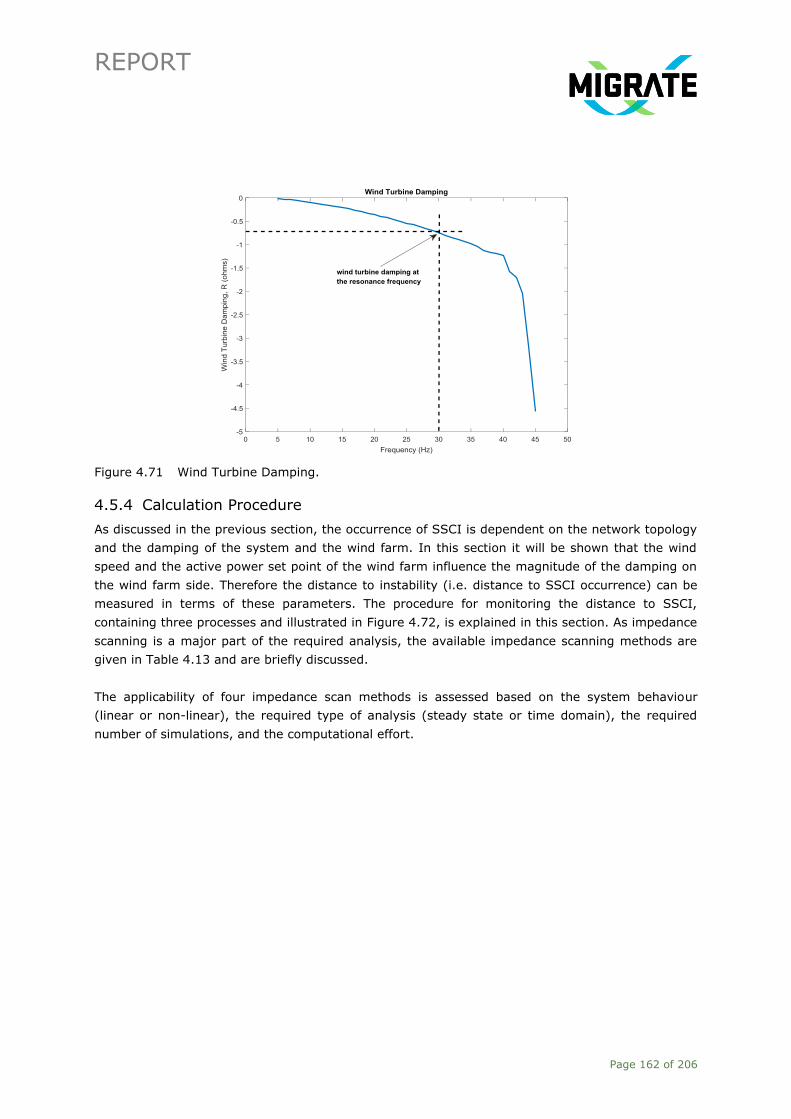
REPORT
Page 162 of 206
Figure 4.71 Wind Turbine Damping.
4.5.4 Calculation Procedure
As discussed in the previous section, the occurrence of SSCI is dependent on the network topology
and the damping of the system and the wind farm. In this section it will be shown that the wind
speed and the active power set point of the wind farm influence the magnitude of the damping on
the wind farm side. Therefore the distance to instability (i.e. distance to SSCI occurrence) can be
measured in terms of these parameters. The procedure for monitoring the distance to SSCI,
containing three processes and illustrated in Figure 4.72, is explained in this section. As impedance
scanning is a major part of the required analysis, the available impedance scanning methods are
given in Table 4.13 and are briefly discussed.
The applicability of four impedance scan methods is assessed based on the system behaviour
(linear or non-linear), the required type of analysis (steady state or time domain), the required
number of simulations, and the computational effort.
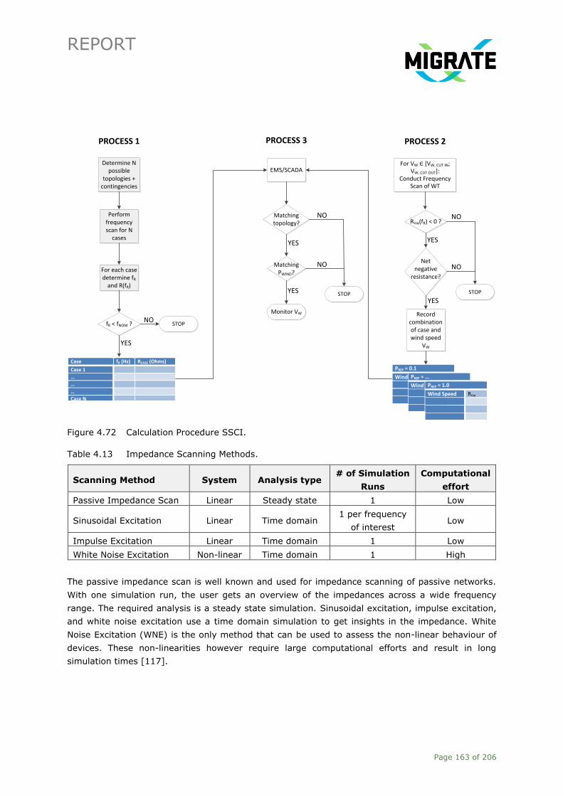
REPORT
Page 163 of 206
Figure 4.72 Calculation Procedure SSCI.
Table 4.13 Impedance Scanning Methods.
Scanning Method System Analysis type # of Simulation
Runs
Computational
effort
Passive Impedance Scan Linear Steady state 1 Low
Sinusoidal Excitation Linear Time domain 1 per frequency
of interest Low
Impulse Excitation Linear Time domain 1 Low
White Noise Excitation Non-linear Time domain 1 High
The passive impedance scan is well known and used for impedance scanning of passive networks.
With one simulation run, the user gets an overview of the impedances across a wide frequency
range. The required analysis is a steady state simulation. Sinusoidal excitation, impulse excitation,
and white noise excitation use a time domain simulation to get insights in the impedance. White
Noise Excitation (WNE) is the only method that can be used to assess the non-linear behaviour of
devices. These non-linearities however require large computational efforts and result in long
simulation times [117].
Determine N possible
topologies + contingencies
Perform frequency scan for N
cases
For each case determine fR
and R(fR)
Case fR (Hz) RCASE (Ohms)
Case 1
…
…
…
Case N
EMS/SCADA
Matching topology?
Matching PWIND?
Monitor VW
NO
NO
NO
STOP
PROCESS 1 PROCESS 3
YES
YES
YES
fR < fNOM ? STOP
For VW ∈ [VW, CUT IN; VW, CUT OUT]:
Conduct Frequency Scan of WT
RVw(fR) < 0 ?
Net negative
resistance?
Record combination of case and wind speed
VW
STOP
NO
NO
PROCESS 2
YES
YES
PREF = 0.1
Wind Speed RVw
PREF = …
Wind Speed RVw
PREF = 1.0
Wind Speed RVw

REPORT
Page 164 of 206
The WNE application in PSCAD consists of 2 modules: the harmonic injection module and the
harmonic measurement module. The harmonic injection can either be a current or voltage injection.
The implemented module contains a spectral voltage injection. The following parameters need to
be defined in this module:
─ Magnitude of the injected voltage ‘Hmag’
The ‘magnitude of the injected signal’ should be large enough to trigger a stable response of the
PEID, yet small enough not to cause any instabilities. Values between 5-10% are suggested.
─ Phase of the injected voltage ‘Ph’ in degrees
This parameter creates a phase shift for each of the injected signals. This spreads out the signal
energy due to which a larger voltage can be injected, without perturbation of the steady state
condition [119].
─ Minimum frequency
─ Maximum frequency
─ Increment of the frequency
The ‘minimum and maximum frequency’ determines the frequency range of interest for the SSCI
investigation, whereas the increment fixes the interval.
The harmonic measurement module measures the current flowing out of the PEID. From the
injected voltages and measured currents the impedance is calculated for each of the frequencies
defined in the harmonic injection module. The parameters that need to be defined here are:
─ Time to record
─ File name
As can be seen from Figure 4.73, the ‘time to record’ is very crucial in terms of accuracy of the
results. After starting the simulations, the model needs to initialise. Only after the breaker that
connects the wind turbine to the network is closed and the transients are stabilised, the currents
can be recorded and processed. It is worth mentioning that this time required for the transients to
stabilise is dependent on the wind speed, active power set point, and the size of the wind farm.
The ‘file name’ is the name of the text file containing the amplitudes and phases of the impedances
at each frequency in the range defined in the harmonic injection module.

REPORT
Page 165 of 206
Figure 4.73 White Noise Excitation Implementation.
For the analysis suggested and carried out in this section, the passive impedance scan and the
white noise excitation method are used for determining the impedances. Figure 4.74 shows the
results of the passive impedance scan and the white noise excitation methods for a passive
network. It can be concluded from this figure that the results are similar when either method is
used on a passive network. This is in line with the results found in [120].
0.0602 [ohm] 0.001916
R=0
SCR 10X/R = 10
DFIGPCCHarm Injectionb a
Harm Measureb a
Bus1D
harm_injection_1...
180
0
Ph
0
deg
10
0
Hmag
0.1
Harmonic Imp
Array - 63VaM
IaM
VaP IaP
Record arreay to fileAL
BL
Array size - 63
@ t - 6.0 sZm
Phm
0.0000
0.0005
0.0010
0.0015
0.0020
0.0025
0.0030
0.0035
0.0040
0.0045
y
freq res Ia

REPORT
Page 166 of 206
Figure 4.74 Impedance Scan Comparison: Passive Impedance Scan vs White Noise Excitation.
The monitoring of SSCI occurrence is defined in 3 processes: the grid side analysis (process 1), the
wind farm side analysis (process 2), and the SSCI monitoring (process 3). Each of these processes
is briefly discussed next.
Process1: Grid side analysis
Process 1 facilitates the frequency scan of the grid. The main goal here is to identify the system
damping at the resonance frequencies of the grid, as seen from the point of common coupling. In
this process it is important to include all relevant grid topologies (including post contingency grid
topologies) that could lead to sub synchronous resonances.
The passive impedance scan can be used for determining the resonance frequencies as well as the
damping on the system side. The justification for using this impedance scanning method is that the
grid is modelled as a passive network.
These analyses will yield a look-up table as shown in Figure 4.75. This table contains for the
defined N grid topologies (Case 1 – Case N) the corresponding resonance frequency (fR) and
associated damping (RCASE). This look-up table will then be used in process 3 for monitoring
purposes.
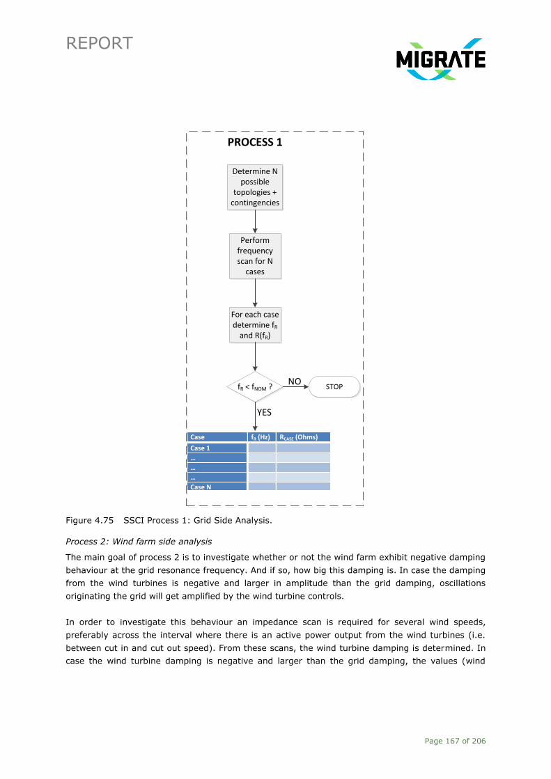
REPORT
Page 167 of 206
Figure 4.75 SSCI Process 1: Grid Side Analysis.
Process 2: Wind farm side analysis
The main goal of process 2 is to investigate whether or not the wind farm exhibit negative damping
behaviour at the grid resonance frequency. And if so, how big this damping is. In case the damping
from the wind turbines is negative and larger in amplitude than the grid damping, oscillations
originating the grid will get amplified by the wind turbine controls.
In order to investigate this behaviour an impedance scan is required for several wind speeds,
preferably across the interval where there is an active power output from the wind turbines (i.e.
between cut in and cut out speed). From these scans, the wind turbine damping is determined. In
case the wind turbine damping is negative and larger than the grid damping, the values (wind
Determine N possible
topologies + contingencies
Perform frequency scan for N
cases
For each case determine fR
and R(fR)
Case fR (Hz) RCASE (Ohms)
Case 1
…
…
…
Case N
NO
PROCESS 1
YES
fR < fNOM ? STOP

REPORT
Page 168 of 206
speed and damping) are recorded and a look-up table is created (see Figure 4.76). This process is
repeated for several levels of active power output of the wind turbines.
Because the wind turbines are active, non-linear components, the passive impedance scan cannot
be used. Instead, the white noise excitation method with harmonic voltage injection is used. As WT
Type 4 wind farms are immune against SSCI ([121], [122], [123]), the focus of the current
analysis is limited to WT Type 3 wind farms.
Figure 4.76 SSCI – Process 2.
Process 3: SSCI monitoring:
The first two processes created look-up tables containing conditions where SSCI might occur. In
the last process the aim is to monitor the system in real-time using these tables. First, the
EMS/SCADA system is used to determine whether the actual grid topology matches one of the N
cases of the took up table created in process 1. Matching topology implies the existence of a
resonance in the sub synchronous frequency range.
For VW ∈ [VW, CUT IN; VW, CUT OUT]:
Conduct Frequency Scan of WT
RVw(fR) < 0 ?
Net negative
resistance?
Record combination of case and wind speed
VW
STOP
NO
NO
PROCESS 2
YES
YES
PREF = 0.1
Wind Speed RVw
PREF = …
Wind Speed RVw
PREF = 1.0
Wind Speed RVw
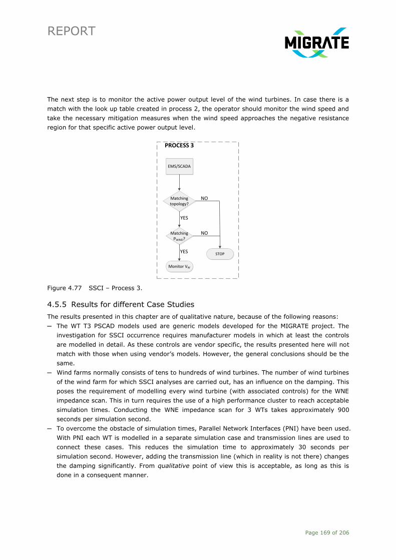
REPORT
Page 169 of 206
The next step is to monitor the active power output level of the wind turbines. In case there is a
match with the look up table created in process 2, the operator should monitor the wind speed and
take the necessary mitigation measures when the wind speed approaches the negative resistance
region for that specific active power output level.
Figure 4.77 SSCI – Process 3.
4.5.5 Results for different Case Studies
The results presented in this chapter are of qualitative nature, because of the following reasons:
─ The WT T3 PSCAD models used are generic models developed for the MIGRATE project. The
investigation for SSCI occurrence requires manufacturer models in which at least the controls
are modelled in detail. As these controls are vendor specific, the results presented here will not
match with those when using vendor’s models. However, the general conclusions should be the
same.
─ Wind farms normally consists of tens to hundreds of wind turbines. The number of wind turbines
of the wind farm for which SSCI analyses are carried out, has an influence on the damping. This
poses the requirement of modelling every wind turbine (with associated controls) for the WNE
impedance scan. This in turn requires the use of a high performance cluster to reach acceptable
simulation times. Conducting the WNE impedance scan for 3 WTs takes approximately 900
seconds per simulation second.
─ To overcome the obstacle of simulation times, Parallel Network Interfaces (PNI) have been used.
With PNI each WT is modelled in a separate simulation case and transmission lines are used to
connect these cases. This reduces the simulation time to approximately 30 seconds per
simulation second. However, adding the transmission line (which in reality is not there) changes
the damping significantly. From qualitative point of view this is acceptable, as long as this is
done in a consequent manner.
EMS/SCADA
Matching topology?
Matching PWIND?
Monitor VW
NO
NO
STOP
PROCESS 3
YES
YES
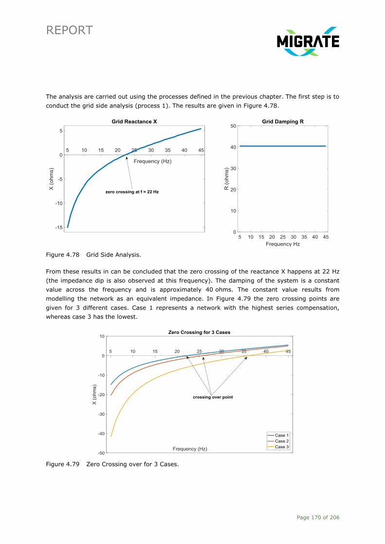
REPORT
Page 170 of 206
The analysis are carried out using the processes defined in the previous chapter. The first step is to
conduct the grid side analysis (process 1). The results are given in Figure 4.78.
Figure 4.78 Grid Side Analysis.
From these results in can be concluded that the zero crossing of the reactance X happens at 22 Hz
(the impedance dip is also observed at this frequency). The damping of the system is a constant
value across the frequency and is approximately 40 ohms. The constant value results from
modelling the network as an equivalent impedance. In Figure 4.79 the zero crossing points are
given for 3 different cases. Case 1 represents a network with the highest series compensation,
whereas case 3 has the lowest.
Figure 4.79 Zero Crossing over for 3 Cases.
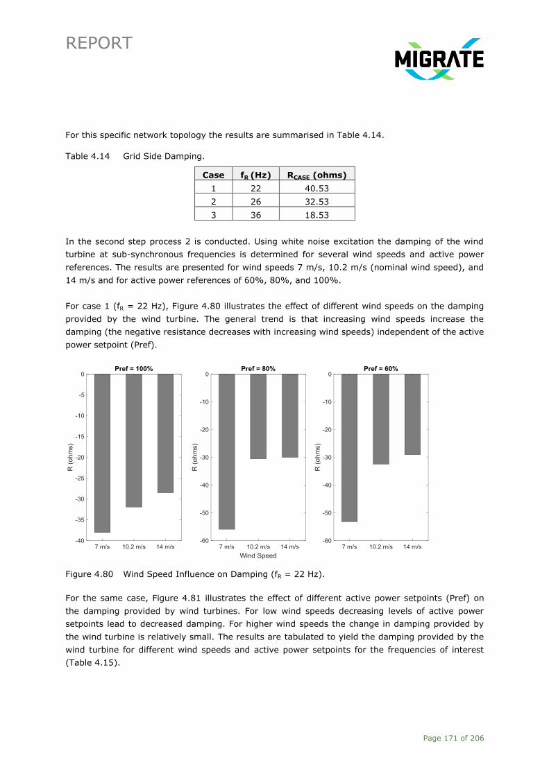
REPORT
Page 171 of 206
For this specific network topology the results are summarised in Table 4.14.
Table 4.14 Grid Side Damping.
Case fR (Hz) RCASE (ohms)
1 22 40.53
2 26 32.53
3 36 18.53
In the second step process 2 is conducted. Using white noise excitation the damping of the wind
turbine at sub-synchronous frequencies is determined for several wind speeds and active power
references. The results are presented for wind speeds 7 m/s, 10.2 m/s (nominal wind speed), and
14 m/s and for active power references of 60%, 80%, and 100%.
For case 1 (fR = 22 Hz), Figure 4.80 illustrates the effect of different wind speeds on the damping
provided by the wind turbine. The general trend is that increasing wind speeds increase the
damping (the negative resistance decreases with increasing wind speeds) independent of the active
power setpoint (Pref).
Figure 4.80 Wind Speed Influence on Damping (fR = 22 Hz).
For the same case, Figure 4.81 illustrates the effect of different active power setpoints (Pref) on
the damping provided by wind turbines. For low wind speeds decreasing levels of active power
setpoints lead to decreased damping. For higher wind speeds the change in damping provided by
the wind turbine is relatively small. The results are tabulated to yield the damping provided by the
wind turbine for different wind speeds and active power setpoints for the frequencies of interest
(Table 4.15).

REPORT
Page 172 of 206
Figure 4.81 Active Power Reference Influence on Damping (fR = 22 Hz).
Table 4.15 Wind Farm Side Damping.
fR = 22 Hz
Pref ↓ 7 m/s 10.2 m/s 14 m/s
100% -38.11 -31.97 -28.56
80% -55.95 -30.61 -30.05
60% -53.26 -32.49 -29.12
fR = 26 Hz
Pref ↓ 7 m/s 10.2 m/s 14 m/s
100% -47 -45.38 -42.21
80% -76.02 -43.30 -40.14
60% -65.82 -44.93 -41.19
fR = 36 Hz
Pref ↓ 7 m/s 10.2 m/s 14 m/s
100% -115 -96.16 -85.50
80% -232.40 -108.46 -77.86
60% -160.21 -111.06 -101.46
As last the impact of the wind farm size on the wind turbine side damping is qualitatively assessed
and illustrated in Figure 4.82. Two important conclusions from these analyses are:
─ The damping provided by the wind farm is proportional to the size of the wind farm.
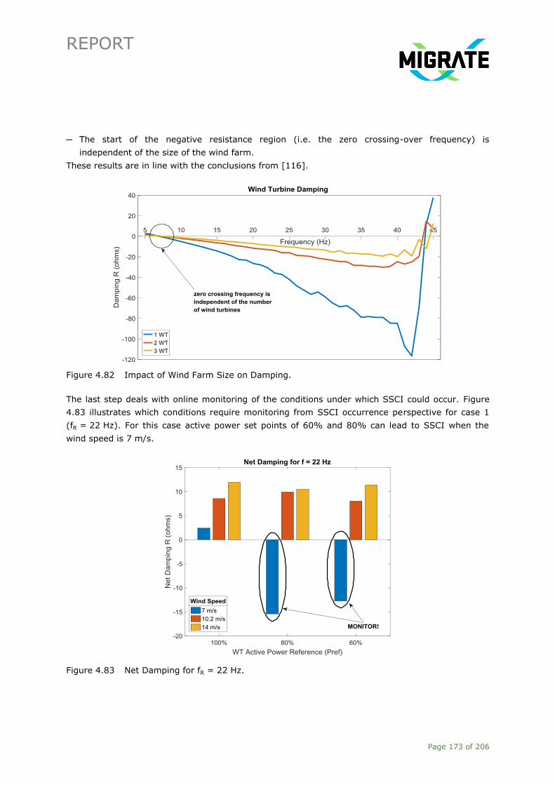
REPORT
Page 173 of 206
─ The start of the negative resistance region (i.e. the zero crossing-over frequency) is
independent of the size of the wind farm.
These results are in line with the conclusions from [116].
Figure 4.82 Impact of Wind Farm Size on Damping.
The last step deals with online monitoring of the conditions under which SSCI could occur. Figure
4.83 illustrates which conditions require monitoring from SSCI occurrence perspective for case 1
(fR = 22 Hz). For this case active power set points of 60% and 80% can lead to SSCI when the
wind speed is 7 m/s.
Figure 4.83 Net Damping for fR = 22 Hz.
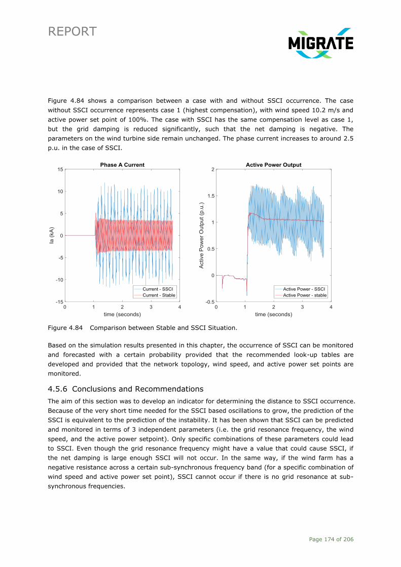
REPORT
Page 174 of 206
Figure 4.84 shows a comparison between a case with and without SSCI occurrence. The case
without SSCI occurrence represents case 1 (highest compensation), with wind speed 10.2 m/s and
active power set point of 100%. The case with SSCI has the same compensation level as case 1,
but the grid damping is reduced significantly, such that the net damping is negative. The
parameters on the wind turbine side remain unchanged. The phase current increases to around 2.5
p.u. in the case of SSCI.
Figure 4.84 Comparison between Stable and SSCI Situation.
Based on the simulation results presented in this chapter, the occurrence of SSCI can be monitored
and forecasted with a certain probability provided that the recommended look-up tables are
developed and provided that the network topology, wind speed, and active power set points are
monitored.
4.5.6 Conclusions and Recommendations
The aim of this section was to develop an indicator for determining the distance to SSCI occurrence.
Because of the very short time needed for the SSCI based oscillations to grow, the prediction of the
SSCI is equivalent to the prediction of the instability. It has been shown that SSCI can be predicted
and monitored in terms of 3 independent parameters (i.e. the grid resonance frequency, the wind
speed, and the active power setpoint). Only specific combinations of these parameters could lead
to SSCI. Even though the grid resonance frequency might have a value that could cause SSCI, if
the net damping is large enough SSCI will not occur. In the same way, if the wind farm has a
negative resistance across a certain sub-synchronous frequency band (for a specific combination of
wind speed and active power set point), SSCI cannot occur if there is no grid resonance at sub-
synchronous frequencies.

REPORT
Page 175 of 206
The proposed methodology for monitoring SSCI consists of 2 phases. The first phase is done offline
and aims to identify which combinations of the parameters could lead to SSCI. For each defined
network topology and active power setpoint, the distance to SSCI occurrence can then be
expressed in terms of the wind speed. The result of the first phase is a set of look-up tables. The
second phase monitors online the 3 parameters and carries out a matching with the look-up tables.
However, unlike e.g. small-disturbance voltage stability where the distance to instability is
expressed in terms of system loading and which can be influenced by the control room operators,
the monitoring variable for SSCI (i.e. the wind speed) cannot be influenced by control room
operators. But, as the wind speed can be forecasted, the distance to SSCI occurrence (i.e.
instability) can be predicted as well, given that the grid resonance frequency and wind turbine
active power setpoint are known.
4.5.7 Control Room Implementation
As the majority of the steps are carried out offline and only the monitoring process is done online,
the proposed method could be implemented in the control room. However, as SSCI is an electrical
(and not an electro-mechanical) phenomenon, the building up of oscillations happens very rapidly.
Therefore it is strongly recommended that for new wind farms SSCI investigations are conducted
and, if SSCI is present, mitigated in the development phase of the project.
The proposed method consists of 3 processes: grid side analysis, wind farm side analysis, and SSCI
monitoring. The grid side analysis results in a look-up table containing the grid resonance
frequencies and associated damping for predefined grid topologies. These analyses are carried out
offline and can be conducted fast.
The wind farm side analysis results in another set of look-up tables containing for each defined grid
resonance frequency the damping of the wind farm for several active power set points. These
analyses are also carried out offline. It should be noted that the damping provided by the wind
farm is heavily dependent on its control algorithms and settings. The studies suggested in this
chapter to determine the wind farm damping should be carried out with detailed manufacturer’s
models instead of generic models, which means that results will be wind farm specific. This step is
very time consuming and cannot be carried out using normal computers. High performance clusters
might help in achieving acceptable simulation times.
In the last process the monitoring is carried out online. The EMS/SCADA can be used to determine
the grid topology. If this grid topology matches with one of the entries of the first look-up table,
the grid resonance frequency can be determined using the same look-up table. The active power
output of the wind farm can be observed from the EMS/SCADA as well. If there is a match with the
second set of look-up tables, the wind speed needs to be monitored.
In terms of implementing this in the control room, an accurate wind forecast is the only missing
component for facilitating the proposed method.

REPORT
Page 176 of 206
A Generic Test Cases
Generic Test Case 1: Frequency Stability
Power System Modelling in PowerFactory
Table A.1 Synchronous generators typical parameters (ElmSym) in generic test case 1.
Parameter Value
Parallel machines 2 – 9
Active power 210 – 240
Reactive power 17 – 100
Voltage 1
Active power limits 80 – 260
Table A.2 Synchronous generators typical parameters (TypSym) in generic test case 1.
Parameter Value
Nominal apparent power 220 – 259
Nominal voltage 15.75
Power factor 0.98
Connection Y
Reactive power limits -130 to 130
Reactance x2 0.2
Resistance r2 0
Inertia constant 6.99 to 10.5
Td’ 0.465
Tq’ 0.188
Td’’ 0.12
Tq’’ 0.188
Xd 1.58
Xq 0.94
Xd’ 0.43
Xq’ 0.54
Xd’’ 0.225
Xq’’ 0.27
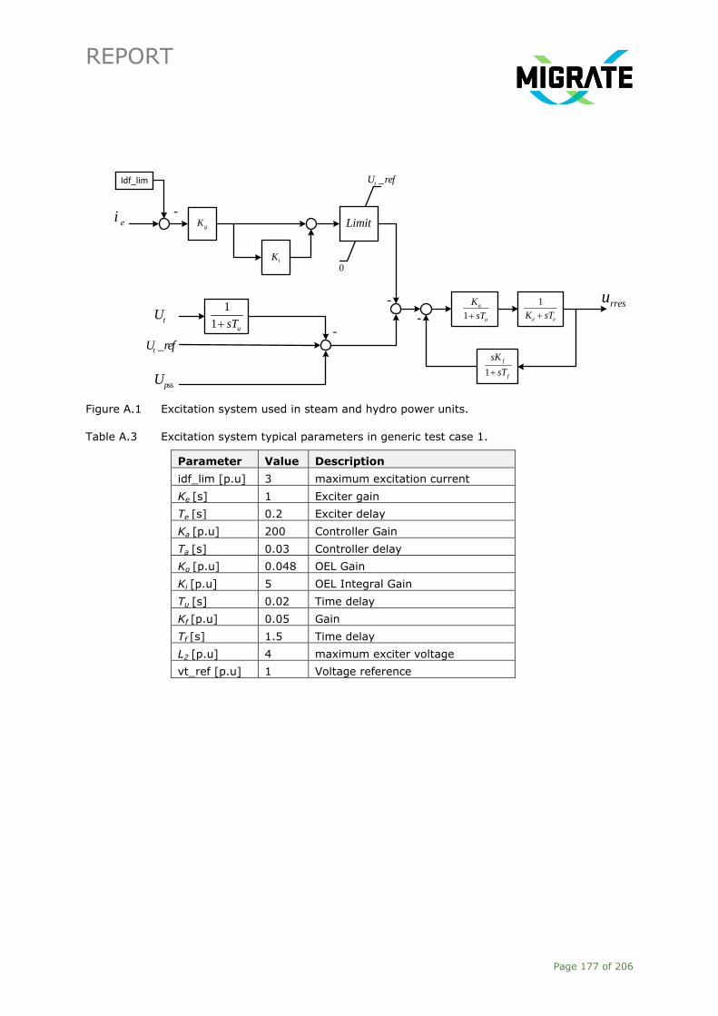
REPORT
Page 177 of 206
Idf_lim
-
-
--
1
1 usT
eigK
iK
1
a
a
K
sT
1
e eK sT
1
f
f
sK
sT
tU
pssU
rresu
0
_tU ref
_tU ref
Limit
Figure A.1 Excitation system used in steam and hydro power units.
Table A.3 Excitation system typical parameters in generic test case 1.
Parameter Value Description
idf_lim [p.u] 3 maximum excitation current
Ke [s] 1 Exciter gain
Te [s] 0.2 Exciter delay
Ka [p.u] 200 Controller Gain
Ta [s] 0.03 Controller delay
Kg [p.u] 0.048 OEL Gain
Ki [p.u] 5 OEL Integral Gain
Tu [s] 0.02 Time delay
Kf [p.u] 0.05 Gain
Tf [s] 1.5 Time delay
L2 [p.u] 4 maximum exciter voltage
vt_ref [p.u] 1 Voltage reference
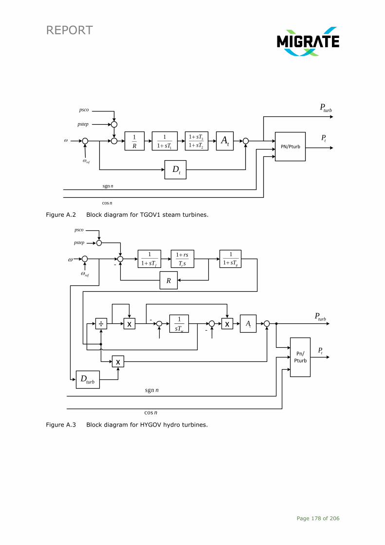
REPORT
Page 178 of 206
PN/Pturb
1
R 1
1
1 sT
3
2
1
1
sT
sT
tA
tD
psco
pstep
ref
sgn n
cos n
tP
turbP
Figure A.2 Block diagram for TGOV1 steam turbines.
-
÷ x x-
-
xPn/
Pturb
1
1 fsT
1
r
rs
T s
1
1 gsT
psco
pstep
ref
R
turbD
1
wsTtA
turbP
tP
sgn n
cos n
Figure A.3 Block diagram for HYGOV hydro turbines.
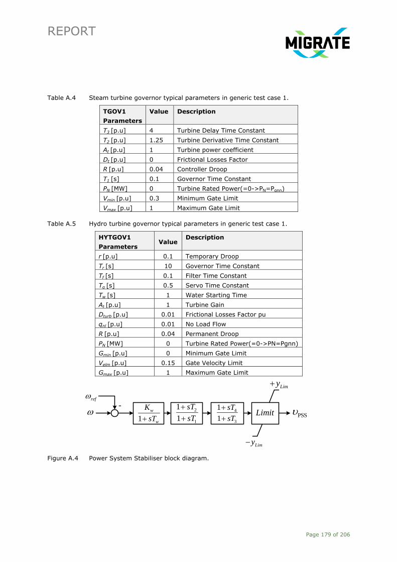
REPORT
Page 179 of 206
Table A.4 Steam turbine governor typical parameters in generic test case 1.
TGOV1
Parameters
Value Description
T3 [p.u] 4 Turbine Delay Time Constant
T2 [p.u] 1.25 Turbine Derivative Time Constant
At [p.u] 1 Turbine power coefficient
Dt [p.u] 0 Frictional Losses Factor
R [p.u] 0.04 Controller Droop
T1 [s] 0.1 Governor Time Constant
PN [MW] 0 Turbine Rated Power(=0->PN=Pgnn)
Vmin [p.u] 0.3 Minimum Gate Limit
Vmax [p.u] 1 Maximum Gate Limit
Table A.5 Hydro turbine governor typical parameters in generic test case 1.
HYTGOV1
Parameters Value
Description
r [p.u] 0.1 Temporary Droop
Tr [s] 10 Governor Time Constant
Tf [s] 0.1 Filter Time Constant
Tg [s] 0.5 Servo Time Constant
Tw [s] 1 Water Starting Time
At [p.u] 1 Turbine Gain
Dturb [p.u] 0.01 Frictional Losses Factor pu
qnl [p.u] 0.01 No Load Flow
R [p.u] 0.04 Permanent Droop
PN [MW] 0 Turbine Rated Power(=0->PN=Pgnn)
Gmin [p.u] 0 Minimum Gate Limit
Velm [p.u] 0.15 Gate Velocity Limit
Gmax [p.u] 1 Maximum Gate Limit
-2
1
1
1
sT
sT
4
3
1
1
sT
sT
1
w
w
K
sT
ref
PSS
Limy
Limy
Limit
Figure A.4 Power System Stabiliser block diagram.

REPORT
Page 180 of 206
Table A.6 PSS typical parameters in generic test case 1.
Parameter Value Description
Kw [p.u] 93.57909 PSS gain
Tw [s] 10 Washout filter time constant
T2 [s] 0.012543 Time constant 2
T1 [s] 0.176775 Time constant 1
T4 [s] 0.014283 Time constant 4
T3 [s] 0.195683 Time constant 3
ylim [p.u] 0.1 Voltage limit
Table A.7 SVSs typical values in generic test case 1.
Parameter Value
Q reactance 700
Max of capacitors 10
Table A.8 Two-winding transformer typical values in generic test case 1.
Parameter (TypTr2) Value
Rated power [MW] 200 - 1000
Nominal frequency [Hz] 50
Rated voltage HV [kV] 20 – 400
Rated voltage LV [kV] 15.75 - 150
Ratio X/R 7 – 50
Short circuit voltage [%] 0.22 – 0.88
Table A.9 General load typical values in generic test case 1.
Parameter Min Value Max value
Active power [MW] 10 800
Reactive power [MW] 20 120
Table A.10 Transmission lines typical values in generic test case 1.
Parameter Min Value
Length [km] 1-220
Parallel lines 1-2
Rated voltage [kV] 110 – 380
Rated current [kA] 1 – 4.08
Nominal frequency [Hz] 50
AC- Resistance [Ohm/km] 0.015 – 0.192
Reactance [Ohm/km] 0.13 – 0.4
Capacitance [uF/km] 0.0085 – 0.0275
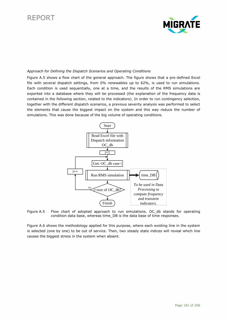
REPORT
Page 181 of 206
Approach for Defining the Dispatch Scenarios and Operating Conditions
Figure A.5 shows a flow chart of the general approach. The figure shows that a pre-defined Excel
file with several dispatch settings, from 0% renewables up to 62%, is used to run simulations.
Each condition is used sequentially, one at a time, and the results of the RMS simulations are
exported into a database where they will be processed (the explanation of the frequency data is
contained in the following section, related to the indicators). In order to run contingency selection,
together with the different dispatch scenarios, a previous severity analysis was performed to select
the elements that cause the biggest impact on the system and this way reduce the number of
simulations. This was done because of the big volume of operating conditions.
Figure A.5 Flow chart of adopted approach to run simulations. OC_db stands for operating condition data base, whereas time_DB is the data base of time responses.
Figure A.6 shows the methodology applied for this purpose, where each existing line in the system
is selected (one by one) to be out of service. Then, two steady state indices will reveal which line
causes the biggest stress in the system when absent.
To be used in Data
Processing to
compute frequency
and transient
indicators.
Start
Read Excel file with
Dispatch information
OC_db
i=1
Get: OC_db case i
time_DB
i=size of OC_db?
i++
NO
Finish
Run RMS simulation

REPORT
Page 182 of 206
Figure A.6 Flow chart to get the elements that cause the biggest impact in steady state conditions. SS_DB stands for data base of steady-state results. PFI denotes power
flow indicator, a measure of the loading of each component.
Start
Lines = get all lines
i=1
Set out of service
Line (i)
i=length(Lines)?
i++
FinishNO
SS_DBRun load
flow
Load
SS_DB
Compute PFI
for all cases
Select highest
PFI and
associated line

REPORT
Page 183 of 206
B Transition Scenario Implementation
B.1 Implementation into the GB Test System
Table B.1 Foreseen Grid Reinforcements in GB Transmission System.
Reinforcement Gone
Green
No
Progression
Reinforced
Boundary
Improvements
in MW
Scotland and North of England
HVDC link Peterhead-
Hawthorn Pit 2023 2029
B2
B4
B5
B6
B7
B7a
300
1360
2000
2010
620
360
Western HVDC Link 2017 N/A
B6
B7
B7a
2200
2500
2830
Series reactors
Reactive compensations
East England
Rayleigh Main series
reactors 2027 N/A EC5 1750
South England
Dynamic reactive
compensation SCVC 2019 2021 SC1 840
West England and North Wales
Carrington series reactor 2023 2020 B8
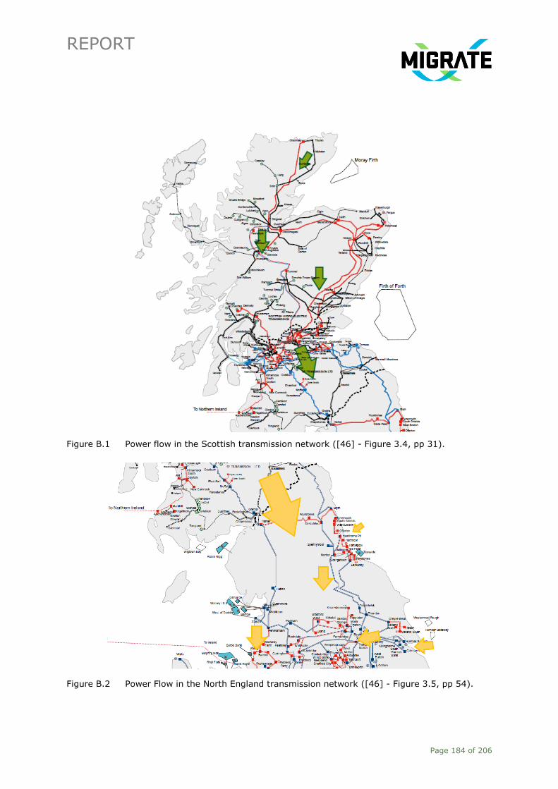
REPORT
Page 184 of 206
Figure B.1 Power flow in the Scottish transmission network ([46] - Figure 3.4, pp 31).
Figure B.2 Power Flow in the North England transmission network ([46] - Figure 3.5, pp 54).

REPORT
Page 185 of 206
Table B.2 Mapping of NOA Boundaries and ETYS Regions to 29 Zone Network Model.
ETYS 2016
Region
ETYS 2016
System Boundary
GB 29 Zone
substation
Scotland
B0 1
B2 2
3
B5
4
5
6
B6 7
8
North England
B7 9
10
B7a 11
EC1 16
West England
NW3 12
B8
13
14
15
B17 17
18
East England EC3
EC5
19
20
South England
B14
21
22
25
SC1
23
24
28
SC2 26
27
B13 29
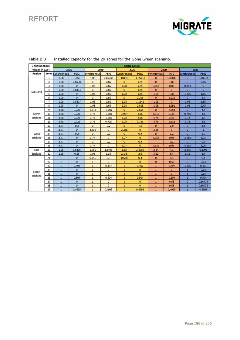
REPORT
Page 186 of 206
Table B.3 Installed capacity for the 29 zones for the Gone Green scenario.
Region Zone Synchronous PEIG Synchronous PEIG Synchronous PEIG Synchronous PEIG Synchronous PEIG
1 1,08 0,856 1,08 0,85033 0,864 1,85033 0 1,85033 0 3,00033
2 1,08 0,8598 0 0,85 0 1,85 0 1,85 0 2,85
3 1,08 0 1,08 0,85 1,08 1,85 0,864 0,85 0,864 0
4 1,08 0,8413 0 0,85 0 1,85 0 0 0 0
5 1,08 0 1,08 0,85 1,08 1,85 1,08 1,85 1,296 1,85
6 1,08 0 0 0,85 0 2,218 0 2,218 0 2,7
7 1,08 0,8427 1,08 0,85 1,08 1,1141 1,08 0 1,08 1,85
8 1,08 0 1,08 0,65 1,08 2,018 1,08 2,291 1,08 2,45
9 3,78 0,725 1,512 1,558 0 2,658 0 2,658 0 4,4
10 3,78 0,725 3,78 1,558 3,024 2,56 1,512 3,35 0,756 4,3
11 3,78 0,725 3,78 1,558 3,78 2,56 3,78 2,56 3,78 3,7
16 3,78 0,725 3,78 0,725 3,78 0,725 3,78 2,332 3,78 2,3
12 3,77 0,2 0 0,2 0 1,9 0 1,9 0 3,4
13 3,77 0 2,639 0 2,268 0 2,18 1 0 1
14 3,77 0,2 0 0,2 0 0,2 0 1,2 0 1,9
15 3,77 0 3,77 0 3,77 0 4,158 0,95 2,268 1,75
17 3,77 0 0 0,2 0 0,2 0,2 0 0,2
18 3,77 0 3,77 0 3,77 0 4,536 0,95 4,158 1,05
19 1,95 0,5495 1,755 1,3495 1,85 2,4995 2,34 4,1 2,145 6,3995
20 1,95 0,55 1,95 1,35 2,145 2,5 3,12 6,4 3,15 6,4
21 1 0 0,756 0,3 0,648 0,4 0 0,4 0 0,4
22 1 0 1 0 1 0 0 0,53 0 0,53
23 1 0,497 1 0,497 1 0,497 1 0,497 1,296 0,497
24 1 0 1 0 1 0 1 0 1 0,53
25 1 0 1 0 1 0 1 0 1 0,53
26 1 0,504 1 0,504 1 0,504 1 0,504 1 0,504
27 1 0 1 0 1 0 1 0,53 0 0,60475
28 1 0 1 0 1 0 1 0,53 1 0,60475
29 1 0,4995 1 0,4995 1 0,4995 1 0,4995 1 0,4995
Scotland
North
England
West
England
East
England
South
England
Generation (all
values in GW)
GONE GREEN
2016 2020 2025 2030 2035

REPORT
Page 187 of 206
Table B.4 Installed capacity for the 29 zones for the No Progression scenario.
Region Zone Synchronous PEIG Synchronous PEIG Synchronous PEIG Synchronous PEIG Synchronous PEIG
1 1,08 0,856 0,86 0,85 0,9 0,85 0,96 0,85 0,84 0
2 1,08 0,8598 0,86 0,85 0,9 0,85 0,96 0,85 0,84 0,85
3 1,08 0 0,86 0 0,9 0 0,96 0,5 0,84 0,5
4 1,08 0,8413 0,86 0,85 0,9 0,85 0,96 0,85 0,84 0,7
5 1,08 0 0,86 0 0,9 0,85 0,96 0,85 0,84 0,85
6 1,08 0 0,86 0 0,9 0,7 0,96 0,7 0,84 0,7
7 1,08 0,8427 0,86 0,85 0,9 0,85 0,96 0,85 0,84 0,85
8 1,08 0 0,86 0,7 0,9 0,85 0,96 0,85 0,84 0,85
9 3,78 0,725 3,15 0,725 4,4 0,725 4,28 0,725 4,03 0
10 3,78 0,725 3,15 0,55825 4,4 0,89175 4,28 1,39275 4,03 1,39275
11 3,78 0,725 3,15 0,55825 4,4 0,89175 4,28 0,89175 4,03 0,89175
16 3,78 0,725 3,15 0,55825 4,4 0,89125 4,28 0,89125 4,03 0,62
12 3,77 0,2 2,93 0,2 1,92 0,2 1,83 0,4 1,83 0,4
13 3,77 0 2,93 0 1,92 0 1,83 0,1 1,83 0,1
14 3,77 0,2 2,93 0,2 1,92 0,2 1,83 0,2 1,83 0,2
15 3,77 0 2,93 0 1,92 0 1,83 0,2 1,83 0,2
17 3,77 0 2,93 0 1,92 0 1,83 0 1,83 0
18 3,77 0 2,93 0 1,92 0,1 1,83 0,1 1,83 0,1
19 1,95 0,5495 2,45 1,0495 2,4 1,0495 2,9 1,0495 2,65 1,0495
20 1,95 0,55 2,45 0,55 2,4 1,15 2,9 1,15 2,65 1,15
21 1 0 0,79 0 1,17 0,105 1,11 0,105 1,12 0,105
22 1 0 0,79 0 1,17 0 1,11 0 1,12 0
23 1 0,497 0,79 0,392 1,17 0,392 1,11 0,392 1,12 0,892
24 1 0 0,79 0 1,17 0 1,11 0 1,12 0
25 1 0 0,79 0 1,17 0 1,11 0 1,12 0
26 1 0,504 0,79 0,504 1,17 0,504 1,11 0 1,12 0
27 1 0 0,79 0 1,17 0 1,11 0 1,12 0,603
28 1 0 0,79 0 1,17 0 1,11 0 1,12 0,3
29 1 0,4995 0,79 0,4995 1,17 0,4995 1,11 0 1,12 0
South
England
Generation per node (all
values in GW) 2030 2035
Scotland
North
England
West
England
East
England
GONE GREEN No Progression
2016 2020 2025

REPORT
Page 188 of 206
B.2 Implementation into the Irish Test System
Table B.5 Ireland ”Slow Change” Scenario.
Demand 2020 2025 2030 2040
Total Data Centre Capacity (MVA) 400 550 850 850
Total number of Electric Vehicles 8000 43000 90000 309000
Total % of Vehicles which are Electric 0% 2% 4% 13%
Total number of Heat Pumps 38000 48000 100000 212000
Total % of Households with Heat Pumps 2% 3% 5% 10%
Total Demand (TWh) 21.2 32.3 35.1 36.6
Generation 2020 2025 2030 2040
Coal 860 860 0 0
Gas 4120 3760 4660 5430
Peat 310 310 0 0
Distillate Oil 410 320 320 0
Heavy Fuel Oil 590 0 0 0
Waste (assume 50% renewable) 80 80 80 100
Fossil fuel generation Total [MW] 6330 5290 5020 5480
Wind (onshore) 3930 4540 4640 4860
Wind (offshore) 30 30 250 500
Wind generation total 3960 4570 4890 5360
Hydro 240 240 240 240
Biomass/Landfill Gas (including Biomass SHP) 240 240 270 410
Solar PV 70 90 200 400
Ocean (Wave/Tidal) 0 0 20 40
Renewable generation Total [MW] 4550 5180 5660 6500
Pumped Storage 290 290 290 290
Small Scale Battery Storage 0 0 50 150
Large Battery Storage 0 0 50 150
Demand Side Management 300 330 400 500
DC Interconnection 500 500 500 1200
Conventional Combined Heat & Power 150 150 150 150
Total Capacity [MW] 12120 11740 12120 14420

REPORT
Page 189 of 206
Table B.6 Ireland ”Low Carbon Living” Scenario.
Demand 2020 2025 2030 2040
Total Data Centre Capacity (MVA) 700 1400 1950 1950
Total number of Electric Vehicles 20000 163000 426000 785000
Total % of Vehicles which are Electric 1% 8% 19% 33%
Total number of Heat Pumps 56000 194000 279000 529000
Total % of Households with Heat Pumps 3% 10% 14% 25%
Total Demand (TWh) 32.6 38.8 43.8 45.8
Generation 2020 2025 2030 2040
Coal 860 0 0 0
Gas 4120 4210 4210 4760
Peat 310 0 0 0
Distillate Oil 410 210 100 0
Heavy Fuel Oil 590 0 0 0
Waste (assume 50% renewable) 80 100 100 100
Fossil fuel generation Total [MW] 6330 4470 4360 4810
Wind (onshore) 4120 5010 5500 6300
Wind (offshore) 30 800 3000 3500
Wind generation total 4150 5810 8500 9800
Hydro 240 240 240 240
Biomass/Landfill Gas (including Biomass SHP) 240 320 750 800
Solar PV 150 700 2500 3500
Ocean (Wave/Tidal) 0 20 100 250
Renewable generation Total [MW] 4820 7140 12140 14640
Pumped Storage 290 290 650 650
Small Scale Battery Storage 0 50 500 800
Large Battery Storage 0 80 1200 1750
Demand Side Management 350 500 750 1250
DC Interconnection 500 1200 1950 1950
Conventional Combined Heat & Power 150 170 180 220
Total Capacity [MW] 12440 13900 21730 26070

REPORT
Page 190 of 206
Table B.7 IEEEX1 AVR model: typical parameters.
Parameter Value Unit Description
Tr 0 [s] Measurement Delay
Ka 50 [pu] Controller Gain
Ta 0.1 [s] Controller Time Constant
Tb 0 [s] Filter Delay Time
Tc 0 [s] Filter Derivative Time Constant
Te 0.5 [s] Exciter Time Constant
Kf 0.04 [pu] Stabilisation Path Gain
Tf1 1 [s] Stabilisation Path Delay Time
E1 1 [pu] Saturation Factor 1
Se1 0 [pu] Saturation Factor 2
E2 1.2 [pu] Saturation Factor 3
Se2 0.1 [pu] Saturation Factor 4
Ke 0 [pu] Exciter Constant
Vrmin -5.4 [pu] Controller Minimum Output
Vrmax 5.4 [pu] Controller Maximum Output
Table B.8 HYGOV governor model: typical parameters.
Parameter Value Unit Description
r 0.5 [pu] Temporary Droop
Tr 10 [s] Governor Time Constant
Tf 0.05 [s] Filter Time Constant
Tg 0.5 [s] Servo Time Constant
Tw 1.3 [s] Water Starting Time
At 1.1 [pu] Turbine Gain
Dturb 0.5 [pu] frictional losses factor pu
qnl 0 [pu] No Load Flow
R 0.04 [pu] Permanent Droop
PN 0 [Mw] Turbine Rated Power(=0->PN=Pgnn)
Gmin 0 [pu] Minimum Gate Limit
Velm 0.2 [pu] Gate Velocity Limit
Gmax 0.76 [pu] Maximum Gate Limit

REPORT
Page 191 of 206
Table B.9 IEEEG2 governor model: typical parameters.
Parameter Value Unit Description
K 22.22 [pu] Controller Gain
T1 0.5 [s] Governor Time Constant
T3 0.35 [s] Servo Time Constant
T2 0.05 [s] Governor Derivative Time Constant
T4 0.1 [s] Water Starting Time
PN 0 [MW] Turbine Rated Power(=0->PN=Pgnn)
Pmin 0.3 [pu] Minimum Gate Limit
Pmax 1 [pu] Maximum Gate Limit
Table B.10 WP controller – WP Q control module.
Name Value Unit Description
rWPdroop 0 [ZWPbase] Resistive component of WP voltage drop impedance
xWPdroop 0 [ZWPbase] Inductive component of WP voltage drop impedance
qinitoffset -1 [PWTN]
Difference between initial p.u. WT output reactive power
and initial p.u. WP output reactive power to compensate
for the losses inside the WP
uWPqdip 0.8 [Un] Voltage threshold for UVRT detection
KWPqu 0 [-] Voltage controller cross coupling gain
Tuqfilt 0.01 [s] Time constant for the UQ static mode
MWPqmode 3 [-]
Reactive power/voltage controller mode (0- reactive
power reference, 1- power factor reference, 2- UQ
static, 3- voltage control)
KPWPx 10 [PWPN/PWTN] Reactive power/voltage PI controller proportional gain
KIWPx 10 [PWP/PWT/s] Reactive power/voltage PI controller integral gain
KWPqref 0 [PWPN/PWTN] Reactive power reference gain
xerrmin -0.4 [PWPN or UN] Minimum reactive power error (or voltage error if
MWPqmode = 2) input to PI controller
KIWPxmin -1 [PWP/PWT/s] Minimum reactive Power/voltage reference from
integration
xrefmin -1 [PWTN] Minimum WT reactive power/voltage reference
xerrmax 0.4 [PWPN or UN] Maximum reactive power error (or voltage error if
MWPqmode = 2) input to PI controller
KIWPxmax 1 [PWP/PWT/s] Maximum reactive Power/voltage reference from
integration
xrefmax 1 [PWTN] Maximum WT reactive power/voltage reference

REPORT
Page 192 of 206
Table B.11 Type 3 and 4 WT controller – Q control module.
Name Value Unit Description
KIq 0 [Un/Pn/s] Reactive power PI controller integrational gain
Tqfiltq 0.01 [s] Reactive power measurement filter time constant
KPq 0 [Un/Pn] Reactive power PI controller proportional gain
MqG 2 [-]
General Q control mode: 0 = voltage, 1 = reacitve
power, 2 = open loop reactive power, 3 = power
factor, 4 = open loop power factor
Tpfiltq 0.005 [s] Power measurement filter time constant
Tqord 10 [s] Time constant in reactive power order lag
uref0 0 [Un] User defined bias in voltage reference uWTref =
uref0+DeltauWTref (used when MqG = MqGu)
KIu 5 [In/Un/s] Voltage PI controller integational gain
KPu 5 [In/Un] Voltage PI controller proportional gain
iqpost 0 [In] Post fault reactive current injection
MqUVRT 1 [-]
UVRT Q control mode: 0 = voltage dependent
reactive current injection, 1 = reactive current as pre-
fault + voltage dependent value, 2 = like 1 but
extended to post-fault
Tufiltq 0.005 [s] Voltage measurement filter time constant
uqdip 0.8 [Un] Voltage threshold for UVRT detection in q control
Tpost 0 [s] Length of time period where post fault reactive power
is injected
udb1 0.9 [Un] Voltage dead band lower limit
udb2 1.1 [Un] Voltage dead band upper limit
Kqv 2 [In/Un] Voltage scaling factor for UVRT current
rdroop 0 [Zbase] Resistive component of voltage drop impedance
xdroop 0 [Zbase] Inductive component of voltage drop impedance
Mcos 0 [-] 0 = cosphi const. or on ext. setpoint, 1 = cosphi
dependent on P, Mcos is only effective if MqG = 3 or 4
u_min 0 [Un] Minimum voltage in voltage PI controller integral term
iq_min -1.05 [In] Minimum reactive current injection
u_max 2 [Un] Maximum voltage in voltage PI controller integral
term
iq_max 1.05 [In] Maximum reactive current injection
iqh1 1.05 [In] Maximum reactive current injection during dip
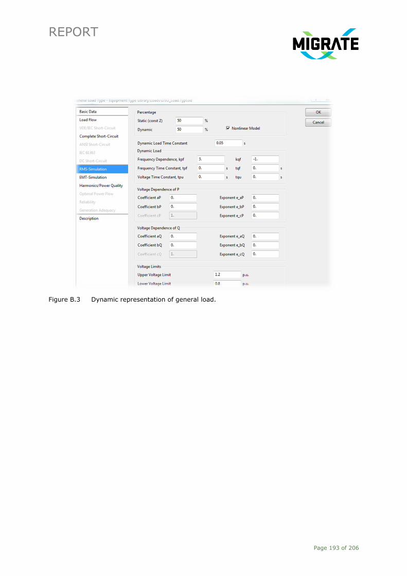
REPORT
Page 193 of 206
Figure B.3 Dynamic representation of general load.

REPORT
Page 194 of 206
C Assessment of KPIs in the Irish System –
Supplementary Information
C.1 Generation Dispatches – WINTER PEAK
Unit name
Aghada AD1.ElmSym 250 200 150 100 100 X X X X X X X
Aghada AT1.ElmSym X X X X X X X X X X X X
Aghada AT2.ElmSym X X X X X X X X X X X X
Aghada AT4.ElmSym X X X X X X X X X X X X
Ardnacrusha AA1.ElmSym 20 20 20 20 20 20 20 20 20 15 X X
Ardnacrusha AA2.ElmSym 20 20 20 20 20 20 20 20 20 15 15 X
Ardnacrusha AA3.ElmSym 20 20 20 20 20 20 20 20 20 15 15 X
Ardnacrusha AA4.ElmSym 20 20 20 20 20 20 20 20 20 15 15 X
Carrigadrohid LE3.ElmSym X X X X X X X X X X X X
Cathaleens Fall ER1.ElmSym X X X X X X X X X X X X
Cathaleens Fall ER2.ElmSym X X X X X X X X X X X X
Cathaleens Fall ER3.ElmSym 20 20 20 20 20 20 20 20 20 15 15 15
Cathaleens Fall ER4.ElmSym 20 20 20 20 20 20 20 20 20 15 15 15
Cushaling ED1.ElmSym 120 120 120 120 120 120 120 120 110 90 X X
Cushaling ED3.ElmSym X X X X X X X X X X X X
Cushaling ED5.ElmSym X X X X X X X X X X X X
Derryiron RP1.ElmSym X X X X X X X X X X X X
Derryiron RP2.ElmSym X X X X X X X X X X X X
Glanagow WG1.ElmSym 400 400 400 400 400 400 400 400 400 380 350 350
Great Island GI4.ElmSym 400 400 400 400 400 400 400 400 400 380 350 350
Huntstown GT HNC.ElmSym 230 230 210 165 X X X X X X X X
Huntstown HN2.ElmSym 380 380 380 380 390 390 390 390 390 380 350 350
Huntstown ST HNC.ElmSym 100 100 80 70 X X X X X X X X
Inniscarra LE1.ElmSym X X X X X X X X X X X X
Inniscarra LE2.ElmSym X X X X X X X X X X X X
Irishtown DB1.ElmSym 400 400 400 400 400 400 400 400 400 380 350 350
Lanesboro LR4.ElmSym 90 90 90 90 90 90 90 90 85 85 85 X
Longpoint AD2.ElmSym 425 425 425 425 425 425 425 425 425 425 425 425
Marina MRT.ElmSym X X X X X X X X X X X X
Moneypoint MP1.ElmSym 275 225 150 150 150 150 160 200 X X X X
Moneypoint MP2.ElmSym 275 225 200 150 150 150 X X X X X X
Moneypoint MP3.ElmSym 275 225 200 150 150 150 160 X X X X X
North Wall NW5.ElmSym X X X X X X X X X X X X
Pollaphuca LI1.ElmSym 14 14 14 14 14 14 14 14 14 10 10 10
Pollaphuca LI2.ElmSym 14 14 14 14 14 14 14 14 14 10 10 10
Pollaphuca LI4.ElmSym 3.5 3.5 3.5 3.5 3.5 3.5 3.5 3.5 3.5 3.5 3.5 3.5
Pollaphuca LI5.ElmSym 3.5 3.5 3.5 3.5 3.5 3.5 3.5 3.5 3.5 3.5 3.5 3.5
Seal Rock SK3.ElmSym 65 65 65 65 65 65 65 65 60 X X X
Seal Rock SK4.ElmSym 65 65 65 65 65 65 65 65 60 50 50 50
Shannonbridge WO4.ElmSym 140 140 140 140 140 140 140 140 120 87 87 X
Shellybanks PB4.ElmSym X X X X X X X X X X X X
Shellybanks PB5.ElmSym 140 115 115 115 115 115 X X X X X X
Shellybanks PB6.ElmSym 150 115 115 115 115 115 115 X X X X X
Tarbert TB1.ElmSym X X X X X X X X X X X X
Tarbert TB2.ElmSym X X X X X X X X X X X X
Tarbert TB3.ElmSym X X X X X X X X X X X X
Tarbert TB4.ElmSym X X X X X X X X X X X X
Tawnaghmore TP1.ElmSym X X X X X X X X X X X X
Tawnaghmore TP3.ElmSym X X X X X X X X X X X X
Turlough Hill TH1.ElmSym 59.46 59.42 60.54 57.84 59.75 58.20 63.32 59.28 59.50 60.34 56.05 56.00
Turlough Hill TH2.ElmSym 60 60 60 60 60 60 60 60 60 60 60 60
Turlough Hill TH3.ElmSym 60 60 60 60 60 60 60 60 60 60 60 60
Turlough Hill TH4.ElmSym 60 60 60 60 60 60 60 60 60 60 60 60
Tynagh CT TYC.ElmSym 250 250 210 160 150 X X X X X X X
Tynagh ST TYC.ElmSym X X X X X X X X X X X X
Synchronous Generator Output [MW]

REPORT
Page 195 of 206
Wind Farm name
ATHEA_DROMADA WP CONTROL.ElmComp 0 12 27 39 54 69 81 93 108 120 135 147
BALLYWATER WP CONTROL.ElmComp 0 6 9 12 15 18 24 27 30 36 39 42
BARNADIVINE WP CONTROL.ElmComp 0 6 12 18 21 27 33 39 45 48 54 60
BOGGERAGH WP CONTROL.ElmComp 0 9 18 27 39 48 57 66 75 87 96 105
BOOLTIAGH WP CONTROL.ElmComp 0 3 6 9 12 15 18 21 24 27 30 33
CASTLEDOCKEREL WP CONTROL.ElmComp 0 6 9 12 15 18 24 27 30 36 39 42
CASTLETOWNMOOR WP CONTROL.ElmComp 0 9 21 33 45 54 66 78 87 99 108 120
CAUTEEN DSO WP CONTROL.ElmComp 0 15 33 45 63 81 96 114 129 144 162 177
CLAHANE WP CONTROL.ElmComp 0 6 9 15 21 24 30 33 39 45 48 54
CLOGHBOOLA DSO WP CONTROL.ElmComp 0 3 6 9 12 15 18 21 24 27 30 33
CLOGHBOOLA WP CONTROL.ElmComp 0 6 9 15 21 27 30 36 42 48 51 57
COOMACHEO WP CONTROL.ElmComp 0 6 12 18 21 27 33 39 45 48 54 60
COOMAGEARLAHY/GLANLEE WP CONTROL.ElmComp 0 9 21 33 45 54 66 78 87 99 108 120
COOMATAGART DSO WP CONTROL.ElmComp 0 6 12 18 24 30 36 42 48 54 60 66
COOMATAGART WP CONTROL.ElmComp 0 9 21 30 42 51 63 72 84 93 105 114
CORDAL DSO WP CONTROL.ElmComp 0 6 12 18 21 27 33 39 45 48 54 60
CORDAL WP CONTROL.ElmComp 0 9 18 27 36 48 54 66 75 84 93 102
CUNGHILL WP CONTROL.ElmComp 0 3 6 12 12 18 18 24 27 30 33 36
DERRYBRIAN WP CONTROL.ElmComp 0 6 12 18 21 27 33 39 45 48 54 60
DONEGAL WP CONTROL.ElmComp 0 15 36 51 72 90 105 123 141 159 177 195
GARVAGH WP CONTROL.ElmComp 0 6 9 15 18 21 27 30 36 39 45 48
IKERRIN DSO WP CONTROL.ElmComp 0 3 6 12 12 18 18 24 27 30 33 36
KILL HILL WP CONTROL.ElmComp 0 6 12 18 21 27 33 39 45 48 54 60
KNOCKACUMMER WP CONTROL.ElmComp 0 9 18 27 39 48 57 66 75 87 96 105
LISHEEN WP CONTROL.ElmComp 0 6 12 18 21 27 33 39 45 48 54 60
MOUNT LUCAS WP CONTROL.ElmComp 0 9 15 21 30 36 45 51 60 66 75 81
RATRUSSAN WP CONTROL.ElmComp 0 9 15 21 30 36 45 51 60 66 75 81
REANMORE DSO WP CONTROL.ElmComp 0 6 12 18 21 27 33 39 45 48 54 60
SLIABH BAWN WP CONTROL.ElmComp 0 6 12 18 21 27 33 39 45 48 54 60
SLIEVE CALLAN WP CONTROL.ElmComp 0 6 12 21 27 36 42 48 54 63 69 75
TRIEN DSO WP CONTROL.ElmComp 0 6 12 18 24 30 36 42 48 54 60 66
WEST GALWAY B WP CONTROL.ElmComp 0 15 30 45 63 78 93 108 123 141 156 171
WEST GALWAY-A WP CONTROL.ElmComp 0 9 18 27 36 45 54 63 72 81 90 99
WEXFORD DSO WP CONTROL.ElmComp 0 3 6 12 15 18 21 24 27 33 36 39
WOODHOUSE WP CONTROL.ElmComp 0 3 3 6 9 9 12 12 15 18 18 21
Combined MW output ==> 0 252 501 756 999 1251 1500 1752 2007 2250 2499 2745
Wind Farm Output [MW]

REPORT
Page 196 of 206
C.2 Generation Dispatches – SUMMER PEAK
Unit name
Aghada AD1.ElmSym X X X X X X X X X X X X
Aghada AT1.ElmSym X X X X X X X X X X X X
Aghada AT2.ElmSym X X X X X X X X X X X X
Aghada AT4.ElmSym X X X X X X X X X X X X
Ardnacrusha AA1.ElmSym 20 20 20 20 20 20 20 20 20 15 X X
Ardnacrusha AA2.ElmSym 20 20 20 20 20 20 20 20 20 15 15 X
Ardnacrusha AA3.ElmSym 20 20 20 20 20 20 20 20 20 15 15 X
Ardnacrusha AA4.ElmSym 20 20 20 20 20 20 20 20 20 15 15 X
Carrigadrohid LE3.ElmSym X X X X X X X X X X X X
Cathaleens Fall ER1.ElmSym X X X X X X X X X X X X
Cathaleens Fall ER2.ElmSym X X X X X X X X X X X X
Cathaleens Fall ER3.ElmSym 20 20 20 20 20 20 20 20 20 15 15 15
Cathaleens Fall ER4.ElmSym 20 20 20 20 20 20 20 20 20 15 15 15
Cushaling ED1.ElmSym 120 120 120 120 120 120 120 120 110 50 X X
Cushaling ED3.ElmSym X X X X X X X X X X X X
Cushaling ED5.ElmSym X X X X X X X X X X X X
Derryiron RP1.ElmSym X X X X X X X X X X X X
Derryiron RP2.ElmSym X X X X X X X X X X X X
Glanagow WG1.ElmSym 400 400 400 400 400 400 400 400 400 380 350 275
Great Island GI4.ElmSym 400 400 400 400 400 400 400 400 345 345 300 275
Huntstown GT HNC.ElmSym 230 200 210 165 X X X X X X X X
Huntstown HN2.ElmSym 390 380 380 280 310 330 390 370 345 300 250 250
Huntstown ST HNC.ElmSym X X X X X X X X X X X X
Inniscarra LE1.ElmSym X X X X X X X X X X X X
Inniscarra LE2.ElmSym X X X X X X X X X X X X
Irishtown DB1.ElmSym 400 400 400 400 400 400 360 300 300 300 250 250
Lanesboro LR4.ElmSym 90 90 90 90 90 90 90 90 85 85 85 X
Longpoint AD2.ElmSym 425 425 425 425 425 425 425 425 425 425 425 425
Marina MRT.ElmSym X X X X X X X X X X X X
Moneypoint MP1.ElmSym 275 225 150 150 150 150 160 X X X X X
Moneypoint MP2.ElmSym 275 225 150 150 150 150 X X X X X X
Moneypoint MP3.ElmSym 275 225 150 150 X X X X X X X X
North Wall NW5.ElmSym X X X X X X X X X X X X
Pollaphuca LI1.ElmSym 14 14 14 14 14 14 14 14 14 10 10 10
Pollaphuca LI2.ElmSym 14 14 14 14 14 14 14 14 14 10 10 10
Pollaphuca LI4.ElmSym 3.5 3.5 3.5 3.5 3.5 3.5 3.5 3.5 3.5 3.5 3.5 3.5
Pollaphuca LI5.ElmSym 3.5 3.5 3.5 3.5 3.5 3.5 3.5 3.5 3.5 3.5 3.5 3.5
Seal Rock SK3.ElmSym 65 65 65 65 65 65 65 65 60 X X X
Seal Rock SK4.ElmSym 65 65 65 65 65 65 65 65 60 50 50 50
Shannonbridge WO4.ElmSym 140 140 140 140 140 140 140 140 X X X X
Shellybanks PB4.ElmSym X X X X X X X X X X X X
Shellybanks PB5.ElmSym 140 115 115 90 115 115 X X X X X X
Shellybanks PB6.ElmSym 150 115 115 115 115 X X X X X X X
Tarbert TB1.ElmSym X X X X X X X X X X X X
Tarbert TB2.ElmSym X X X X X X X X X X X X
Tarbert TB3.ElmSym X X X X X X X X X X X X
Tarbert TB4.ElmSym X X X X X X X X X X X X
Tawnaghmore TP1.ElmSym X X X X X X X X X X X X
Tawnaghmore TP3.ElmSym X X X X X X X X X X X X
Turlough Hill TH1.ElmSym 57.3 51.6 53.8 53.7 56.2 59.7 54.4 53.9 53.7 54.1 61.7 56.7
Turlough Hill TH2.ElmSym 60 60 60 60 60 60 60 60 60 60 60 60
Turlough Hill TH3.ElmSym 60 60 60 60 60 60 60 60 60 60 60 60
Turlough Hill TH4.ElmSym 60 60 60 60 60 60 60 60 60 60 60 60
Tynagh CT TYC.ElmSym 250 250 210 130 150 X X X X X X X
Tynagh ST TYC.ElmSym X X X X X X X X X X X X
Synchronous Generator Output [MW]

REPORT
Page 197 of 206
Wind Farm name
ATHEA_DROMADA WP CONTROL.ElmComp 0 12 27 39 54 69 81 93 108 120 135 147
BALLYWATER WP CONTROL.ElmComp 0 6 9 12 15 18 24 27 30 36 39 42
BARNADIVINE WP CONTROL.ElmComp 0 6 12 18 21 27 33 39 45 48 54 60
BOGGERAGH WP CONTROL.ElmComp 0 9 18 27 39 48 57 66 75 87 96 105
BOOLTIAGH WP CONTROL.ElmComp 0 3 6 9 12 15 18 21 24 27 30 33
CASTLEDOCKEREL WP CONTROL.ElmComp 0 6 9 12 15 18 24 27 30 36 39 42
CASTLETOWNMOOR WP CONTROL.ElmComp 0 9 21 33 45 54 66 78 87 99 108 120
CAUTEEN DSO WP CONTROL.ElmComp 0 15 33 45 63 81 96 114 129 144 162 177
CLAHANE WP CONTROL.ElmComp 0 6 9 15 21 24 30 33 39 45 48 54
CLOGHBOOLA DSO WP CONTROL.ElmComp 0 3 6 9 12 15 18 21 24 27 30 33
CLOGHBOOLA WP CONTROL.ElmComp 0 6 9 15 21 27 30 36 42 48 51 57
COOMACHEO WP CONTROL.ElmComp 0 6 12 18 21 27 33 39 45 48 54 60
COOMAGEARLAHY/GLANLEE WP CONTROL.ElmComp 0 9 21 33 45 54 66 78 87 99 108 120
COOMATAGART DSO WP CONTROL.ElmComp 0 6 12 18 24 30 36 42 48 54 60 66
COOMATAGART WP CONTROL.ElmComp 0 9 21 30 42 51 63 72 84 93 105 114
CORDAL DSO WP CONTROL.ElmComp 0 6 12 18 21 27 33 39 45 48 54 60
CORDAL WP CONTROL.ElmComp 0 9 18 27 36 48 54 66 75 84 93 102
CUNGHILL WP CONTROL.ElmComp 0 3 6 12 12 18 18 24 27 30 33 36
DERRYBRIAN WP CONTROL.ElmComp 0 6 12 18 21 27 33 39 45 48 54 60
DONEGAL WP CONTROL.ElmComp 0 15 36 51 72 90 105 123 141 159 177 195
GARVAGH WP CONTROL.ElmComp 0 6 9 15 18 21 27 30 36 39 45 48
IKERRIN DSO WP CONTROL.ElmComp 0 3 6 12 12 18 18 24 27 30 33 36
KILL HILL WP CONTROL.ElmComp 0 6 12 18 21 27 33 39 45 48 54 60
KNOCKACUMMER WP CONTROL.ElmComp 0 9 18 27 39 48 57 66 75 87 96 105
LISHEEN WP CONTROL.ElmComp 0 6 12 18 21 27 33 39 45 48 54 60
MOUNT LUCAS WP CONTROL.ElmComp 0 9 15 21 30 36 45 51 60 66 75 81
RATRUSSAN WP CONTROL.ElmComp 0 9 15 21 30 36 45 51 60 66 75 81
REANMORE DSO WP CONTROL.ElmComp 0 6 12 18 21 27 33 39 45 48 54 60
SLIABH BAWN WP CONTROL.ElmComp 0 6 12 18 21 27 33 39 45 48 54 60
SLIEVE CALLAN WP CONTROL.ElmComp 0 6 12 21 27 36 42 48 54 63 69 75
TRIEN DSO WP CONTROL.ElmComp 0 6 12 18 24 30 36 42 48 54 60 66
WEST GALWAY B WP CONTROL.ElmComp 0 15 30 45 63 78 93 108 123 141 156 171
WEST GALWAY-A WP CONTROL.ElmComp 0 9 18 27 36 45 54 63 72 81 90 99
WEXFORD DSO WP CONTROL.ElmComp 0 3 6 12 15 18 21 24 27 33 36 39
WOODHOUSE WP CONTROL.ElmComp 0 3 3 6 9 9 12 12 15 18 18 21
Combined MW output ==> 0 252 501 756 999 1251 1500 1752 2007 2250 2499 2745
Wind Farm Output [MW]

REPORT
Page 198 of 206
D Use of Inertia for Frequency Stability KPI As it was explained in Section 4.2.1, i.e. equation (4.3), the inertia H [s] is proportionally related to
the Kinetic Energy [MW.s]. Figure D.1 and Figure D.2 below constitute an alternative
representation to Figure 4.13 and Figure 4.14 for Generic Test Case 1 (cf. Section 4.2.2). By
comparing Figure D.1 and Figure D.2 with Figure 4.13 and Figure 4.14, it can be seen that similar
patterns are found when analysing ROCOF/Nadir with respect to different values of system Kinetic
Energy or System Inertia (Hsys). The system inertia is computed by summing up all the inertia
constants of the generators in service in each operational scenario (cf. Section 4.2.2).
Figure D.1 ROCOF vs Inertia, generic test case 1.
Figure D.2 NADIR vs Inertia, generic test case 1.
0
0,05
0,1
0,15
0,2
0,25
0,3
0 100 200 300 400 500 600 700
RO
CO
F [H
z/s]
Hsys [s]
Winter
Spring
Summer
49,78
49,8
49,82
49,84
49,86
49,88
49,9
49,92
0 100 200 300 400 500 600 700
NA
DIR
[H
z]
Hsys [S]
Winter
Spring
Summer

REPORT
Page 199 of 206
Bibliography [1] MIGRATE consortium, “MIGRATE Grant Agreement,” , MIGRATE consortium, 2015.
[2] MIGRATE Work Package 1 – responsible partner: TenneT, “MIGRATE Deliverable 1.1: Report
on Systemic Issues,” MIGRATE consortium, 2016.
[3] P. Kundur, et al., "Definition and classification of power system stability IEEE/CIGRE joint task
force on stability terms and definitions," in IEEE Transactions on Power Systems, vol. 19, no. 3,
pp. 1387-1401, Aug. 2004.
[4] M. Pöller, “Analyse von Ausgleichsvorgängen in Elektroenergiesystemen unter besonderer
Berücksichtigung des Multiple-Time-Scale-Verhaltens,” Fortschritt-Berichte VDI, VDI-Verlag,
Düsseldorf, 2001.
[5] B. Oswald and D. Siegmund, Berechnung von Ausgleichsvorgängen in Elektroenergiesystemen.
Deutscher Verlag für Grundstoffindustrie, Leipzig, 1991.
[6] J. R. Winkelman, J. H. Chow, J. J. Allemong, and P. V. Kokotovic, “Multi-time-scale Analysis of
a power system,” in Automatica, Vol. 16, pp. 35-43, Pergamon Press Ltd., 1980.
[7] J. H. Chow, Time scale Modelling of Dynamic Networks with Applications to power systems.
Springer-Verlag, Berlin/Heidelberg/New York, 1982.
[8] L. Hofmann, “Effiziente Berechnung von Ausgleichsvorgängen in ausgedehnten
Elektroenergiesystemen,” Habilitationsschrift Universität Hannover, Shaker Verlag, 2003.
[9] DIgSILENT GmbH, “PowerFactory Version 2017 User Manual” Online Edition, DIgSILENT GmbH,
Gomaringen, Germany, December 2016.
[10] P. Ferracci, “Ferroresonance,” in Cahier technique, no. 190, Group Schneider, March 1998.
[11] P. W. Sauer, "Time-scale features and their applications in electric power system dynamic
modeling and analysis," in Proceedings of the 2011 American Control Conference, San
Francisco, CA, 2011. Available online at: http://ieeexplore.ieee.org/ [Last accessed: 5 April
2016].
[12] P. Kundur, Power System Stability and Control. McGraw-Hill, USA, 1994.
[13] V. Crastan and D. Westermann, Elektrische Energieversorgung 3. 3rd edition, Springer-Verlag,
2012.
[14] Enercon GmbH, “Integrated solutions for compliance with demanding international grid codes,”
2016. Available online at: http://www.enercon.de/en/technology/grid-technology/ [Last
accessed: 16 March 2017].
[15] ENTSO-E, “Requirements on the Context of Present Practices,” 26 June 2012. Available online
at: http://www.acer.europa.eu/Media/News/Documents/120626%20-%20NC%20RfG%20-%
20Requirements%20in%20the%20context%20of%20present%20practices.pdf [Last accessed
23 August 2016].
[16] DIgSILENT GmbH, “DIgSILENT PowerFactory Technical Reference Documentation –
Synchronous Machine ElmSym, TypSym,” Gomaringen, Germany, 2016.
[17] DIgSILENT GmbH, “DIgSILENT PowerFactory 2016 – User Manual,” Gomaringen, Germany,
July 2016.
[18] DIgSILENT GmbH, “DIgSILENT PowerFactory Technical Reference Documentation –SVS Static
Var System ElmSvs,” Gomaringen, Germany, 2016.

REPORT
Page 200 of 206
[19] DIgSILENT GmbH, “DIgSILENT PowerFactory Technical Reference Documentation – Two-
Winding Transformer (3-Phase) ElmTr2,TypTr2,” Gomaringen, Germany, 2016.
[20] DIgSILENT GmbH, “DIgSILENT PowerFactory Technical Reference Documentation – General
Load ElmLod, TypLod,” Gomaringen, Germany, 2016.
[21] DIgSILENT GmbH, “DIgSILENT PowerFactory Technical Reference Documentation –
Overhead Line Models ElmLne, TypLne, TypGeo, TypTow,” Gomaringen, Germany, 2015.
[22] DIgSILENT GmbH, “DIgSILENT PowerFactory 2016 – User Manual,” Gomaringen, Germany,
July 2016.
[23] Q. Shafiee, J.M. Guerrero, and J.C. Vasquez, "Distributed Secondary Control for Islanded
Microgrids—A Novel Approach," IEEE Transactions on Power Systems, Vol. 29, No. 2, Feb.
2014.
[24] DIgSILENT GmbH, “DIgSILENT PowerFactory Technical Reference Documentation – Phase
Measurement Device, ElmPhi_pll,” Gomaringen, Germany, 2016.
[25] Energynautics, “MIGRATE Project, Type-3 and Type-4 EMT – Model Documentation”,
Darmstadt, Germany, 2017.
[26] IEC, “IEC standard 61400-27-1, Wind turbines – Part 27-1: Electrical simulation
models - Wind turbines” Edition 1, 2015.
[27] IEC, “IEC standard 61400-27-1, Wind turbines – Part 27-1: Electrical simulation
models - Wind turbines” Edition 2, 2017.
[28] Tennet TSO GmbH, “Grid Code High and Extra High Voltage (onshore),” no. November, pp.
1–46, 2015.
[29] J. Schmidt, E. Tröster, G. Papaioannou, and J. Hanson, “Frequency Issues of Island Power
Systems with High Penetration of Hydroelectric and Wind Power,” 12th Wind Integr. Work.
[30] S. Engelken, A. Mendonca, and M. Fischer, “Inertial Response with Improved Variable
Recovery Behaviour Provided by Type 4 Wind Turbines,” 14th Wind Integr. Work.
[31] Manitoba HVDC Research Centre, „User's Guide on the use of PSCAD,” Manitoba HVDC
Research Centre, Winnipeg, 2016.
[32] Manitoba HVDC Research Centre, „User's Guide. A Comprehensive Resource for EMTDC,”
Manitoba HVDC Research Centre, Winnipeg, 2010.
[33] Manitoba HVDC Research Centre, “MIGRATE Project, Type-3 and Type-4 EMT Model
Documentation”, 23 January 2017.
[34] J. L. Rueda, J. C. Cepeda, I. Erlich, A. W. Korai, and F. M. Gonzalez-Longatt, Probabilistic
Approach for Risk Evaluation of Oscillatory Stability in Power Systems - PowerFactory
Applications for Power System Analysis. pp. 249-266, Springer International Publishing, 2014.
[35] P. Teeuwsen, “Oscillatory stability assessment of power systems using computational
intelligence,” PhD Dissertation, University Duisburg-Essen, 2005.
[36] P. Teeuwsen, I. Erlich, M. El-Sharkawi, and U. Bachmann, “Genetic algorithm and decision
tree based oscillatory stability assessment,” in IEEE Russia Power Tech, pp. 1-7, 2005.
[37] V. Yaramasu, B. Wu, P. C. Sen, S. Kouro, and M. Narimani, "High-power wind energy
conversion systems: State-of-the-art and emerging technologies," in Proceedings of the IEEE,
vol. 103, no. 5, pp. 740-788, May 2015.

REPORT
Page 201 of 206
[38] F. Shewarega, I. Erlich, and J. L. Rueda, "Impact of large offshore wind farms on power
system transient stability," 2009 IEEE/PES Power Systems Conference and Exposition,
Seattle, WA, pp. 1-8, 2009.
[39] ENTSO-E, “Frequency Stability Evaluation Criteria for the Synchronous Zone of Continental
Europe,” ENTSO-E, 2016
[40] Center for Intelligent Systems & Networks, „Dynamic IEEE Test Systems,” Center for
Intelligent Systems & Networks, Available online at: http://www.kios.ucy.ac.cy/testsystems/
index.php/dynamic-ieee-test-systems/ieee-9-bus-modified-test-system [Last accessed: 29
September 2017].
[41] IEEE Subsynchronous Resonance Task Force, “First benchmark model for computer
simulation of subsynchronous resonance,” in IEEE Transactions on Power Apparatus and
Systems, vol. 96, nr. 5, pp. 1565-1572, 1977.
[42] J. Garcia, K. Mudunkotuwa, and C. Shumski, “MIGRATE project – Type-3 and Type-4 EMT
model documentation,” Manitoba HVDC Research Centre, Winnipeg, 2017.
[43] Cambridge, “Cambridge Dictionary,” Available online at: http://dictionary.cambridge.org/
dictionary/english/transition [Last accessed: 24 May 2017].
[44] J. Grin, J. Rotmans, and J. Schot, Transition to Sustainable Development. New Directions in
the Study of Long Term Transformative Change. Oxon: Taylor & Francis, 2010.
[45] National Grid, “Network Options Assessment 1,” National Grid plc, Warwick, 2016.
[46] National Grid, “Electricity Ten Year Statement 2016 – UK electricity transmission,” National
Grid plc, Warwick, 2016.
[47] ENTSO-E, “Scenario Outlook & Adequacy Forecast,” ENTSO-E, Brussels, 2015.
[48] National Grid, “Future Energy Scenarios,” National Grid plc, Warwick, 2015.
[49] L. Shen, “Model integration and control interaction analysis of ac/vsc hvdc system,” Non-
published work, 2015.
[50] ENTSO-E, “New Scenario outlook and adequacy forecast 2015,” ENTSO-E, 2015.
[51] D. Cai, “Wide area monitoring, protection and control in the future great Britain power
system,” PhD dissertation, The University of Manchester, Manchester, 2012.
[52] Cigre WG C4.605, “Modelling and aggregation of loads in flexible power networks,” Available
online at: http://c4.cigre.org/WG-Area/WG-C4.605-Modelling-and-aggregation-of-loads-in-
flexible-power-networks [Last accessed: December 2017].
[53] D. Gusain, J. L. Rueda, J. C. Boemer, and P Palensky, “Identification of Dynamic Equivalents
of Active Distribution Networks Through MVMO,” in IFAC Workshop on Control of
Transmission and Distribution Smart Grids (CTDSG), 2016.
[54] F. Shewarega, I. Erlich, and J. L. Rueda, “Impact of large offshore wind farms on power
system transient stability,” in IEEE/PES Power Systems Conference and Exposition, pp. 1–8,
2009.
[55] EirGrid Group, “All-Island Ten Year Transmission Forecast Statement,” EirGrid Group, Dublin,
2015. Available online at: www.eirgridgroup.com
[56] EirGrid Group, “Tomorrow’s Energy Scenarios 2017. Planning our Energy Future,” EirGrid
Group, Dublin, Available online at http://www.eirgridgroup.com/site-files/library/EirGrid/
EirGrid-Tomorrows-Energy-Scenarios-Report-2017.pdf

REPORT
Page 202 of 206
[57] EirGrid Group, “Grid Code in Ireland,” EirGrid Group, Dublin, 2015. Available online at:
http://www.eirgridgroup.com/site-files/library/EirGrid/GridCodeVersion6.pdf
[58] Australian Energy Market Commission (AEMC), “FFR feasibility assessment,” AEMC, Sydney,
Australlia, 2017. Available online at: http://www.aemc.gov.au/Markets-Reviews-
Advice/System-Security-Market-Frameworks-Review.
[59] ENTSO-E, “Continental Europe Operation Handbook, Policy 1: Load-Frequency Control and
Performance – Appendix,” Tech. Rep., ENTSO-E, Brussels, Belgium, March 2016.
[60] H. Chavez and R. Baldick, “Inertia and governor ramp rate constrained economic dispatch to
assess primary frequency response adequacy,” in International Conference on Renewable
Energies and Power Quality (ICREPQ12), pp. 1–6, March 2012.
[61] P. Tielens, “Operation and Control of Power Systems with Low Synchronous Inertia,” PhD
dissertation, KU Leuven, November 2017.
[62] U. Rudez and R. Mihalic, "Monitoring the First Frequency Derivative to Improve Adaptive
Underfrequency Load-Shedding Schemes," IEEE Transactions on Power Systems, vol. 26, no.
2, pp. 839-846, May 2011.
[63] E. Ørum et al, “Future system inertia,” ENTSO-E NORDIC report, last update: November
2015. Available online at: https://www.entsoe.eu/Documents/Publications/SOC/Nordic/
Nordic_report_Future_System_Inertia.pdf
[64] I. Dudurych, M. Burke, L. Fisher, M. Eager, and Kieran Kelly, “Operational security challenges
and tools for a synchronous power system with high penetration of non-conventional
sources,” in CIGRE Science & Engineering, no. 7, pp. 91-101, Feb. 2017.
[65] V.V. Terzija, “Adaptive Underfrequency Load Shedding Based on the Magnitude of the
Disturbance Estimation”, IEEE Transactions on Power Systems, Vol. 21, No. 3, pp. 1260-
1266, August, 2006.
[66] A. Ulbig, T. S. Borsche, and G. Andersson, “Impact of Low Rotational Inertia on Power
System Stability and Operation,” Proceedings of the 19th World Congress International
Federation of Automatic Control, vol. 47, no. 3, 2014, pp. 7290-7297 Cape Town, South
Africa, August 24-29, 2014.
[67] L. Ruttledge and D. Flynn, “Short-term frequency response of power systems with high non-
synchronous penetration levels,” Wiley Interdisciplinary Reviews: Energy and Environment,
vol. 4, no. 5, pp. 452–470, 2015.
[68] H. Chavez, R. Baldick, and S. Sharma, “Governor rate-constrained OPF for primary frequency
control adequacy,” IEEE Transactions on Power Systems, vol. 29, no. 3, pp. 1473–1480, May
2014.
[69] J.V. Milanovic, et al., “CIGRE WG C4.605: Modelling and aggregation of loads in flexible
power networks,” Cigré, 2014.
[70] J. V. Milanovic, K. Yamashita, S. Martínez Villanueva, S. Ž. Djokic, L. M. Korunović,
“International Industry Practice on Power System Load Modeling,” IEEE Transactions on
Power Systems, Vol. 28, Issue: 3, pp. 3038-3046, 2013.
[71] S. Wellhöfer, S. Höhn, and M. Luther, “Impact of load modeling on small signal stability
investigations,” in IEEE International Conference on Power System Technology (POWERCON),
pp. 1-6. Wollongong, Australia, 2016.

REPORT
Page 203 of 206
[72] A.Nechifor, M.Albu, R.Hair, and V.Terzija, “A flexible platform for synchronized
measurements, data aggregation and information retrieval”, in Electric Power Systems
Research, vol. 120, pp. 20, 31, March, 2015.
[73] M. De Cristofaro, N. Femia, G. Petrone, G. Buticchi, G. De Carne, and M. Liserre, "The Effect
of a Constant Power Load on the Stability of a Smart Transformer,” in IEEE 13th
International Conference on Industrial Informatics (INDIN’155), 2015.
[74] A. Li and Z. Cai, “A method for frequency dynamics analysis and load shedding assessment
based on the trajectory of power system simulation,” in 3rd International Conf. on Electric
Utility Deregulation and Restructuring and Power Technologies (DRPT), pp. 1335-1339, 2008.
[75] K. Das, J. Hazra, D.P. Seetharam, R. K. Reddi, and A. K. Sinha, "Real-time hybrid state
estimation incorporating SCADA and PMU measurements," in 3rd IEEE PES Innovative Smart
Grid Technologies Europe (ISGT Europe), pp.1-8, 2012.
[76] A. E. Leon, J. M. Mauricio, A. Gomez-Exposito, and J. A. Solsona, "Hierarchical Wide-Area
Control of Power Systems Including Wind Farms and FACTS for Short-Term Frequency
Regulation,” in IEEE Transactions on Power Systems, Vol. 27, No. 4, pp. 2084-2092, 2012.
[77] F. Aminifar, M. Fotuhi-Firuzabad, A. Safdarian, A. Davoudi, and M. Shahidehpour,
"Synchrophasor Measurement Technology in Power Systems: Panorama and State-of-the-
Art," in IEEE Access, vol. 2, pp. 1607-1628, 2014.
[78] S. Jin, Z. Huang, R. Diao, D. Wu, and Y. Chen, "Comparative Implementation of High
Performance Computing for Power System Dynamic Simulations," in IEEE Transactions on
Smart Grid, vol. 8, no. 3, pp. 1387-1395, May 2017.
[79] P. Palensky, A. A. Van Der Meer, C. D. Lopez, A. Joseph, and K. Pan, "Cosimulation of
Intelligent Power Systems: Fundamentals, Software Architecture, Numerics, and Coupling,"
in IEEE Industrial Electronics Magazine, vol. 11, no. 1, pp. 34-50, March 2017.
[80] EirGrid Group, “DS3: Rate of Change of Frequency Workstream,” EirGrid Group, Dublin, 2011.
Available online at: http://www.eirgridgroup.com/site-files/library/EirGrid/DS3-Rate-of-
Change-of-Frequency-(RoCoF)Workstream-Plan-2011.pdf
[81] EirGrid Group, “RoCoF Alternative and Solutions Project – Phase 2 Study Report,” EirGrid
Group, Dublin, 2016. Available online at: http://www.eirgridgroup.com/site-files/library/
EirGrid/RoCoF-Alternative-Solutions-Project-Phase-2-Report-Final.pdf
[82] Australian Energy Market Operator (AEMO), “Technology Capabilities for Fast Frequency
Response”, AEMO, Schenectady, Australia, 2017. Available online at:
https://www.aemo.com.au/-/media/Files/Electricity/NEM/Security_and_Reliability/Reports/
2017-03-10-GE-FFR-Advisory-Report-Final---2017-3-9.pdf
[83] North America Electric Reliability Corporation (NERC), “Frequency Response Initiative Report
– The Reliability Role of Frequency Response,” NERC, Atlanta, GA, 2012. Available online at:
http://www.nerc.com/docs/pc/FRI_Report_10-30-12_Master_w-appendices.pdf
[84] R. Bank Tavakoli, M. Power, L. Rutledge, and D. Flynn, “Load inertia estimation using white
and grey-box estimators for power systems with high wind generation,” in IFAC Power Plant
and Power System Control Symposium Toulouse, France, Sept 2012.

REPORT
Page 204 of 206
[85] T. Inoue, H. Taniguchi, Y. Ikeguchi, and K. Yoshida, “Estimation of power system inertia
constant and capacity of spinning-reserve support generators using measured frequency
transients,” in IEEE Transactions on Power Systems, Vol. 13, no. 1, pp. 136-143, 1997.
[86] M. Oluic, M. Ghandhari, and B. Berggren, “Methodology for Rotor Angle Transient Stability
Assessment in Parameter Space,” in IEEE transactions on Power Systems, vol.32, no. 2,
pp. 1202-1211, March, 2017.
[87] F. G. Velez, V. A. Centeno, A. G. Phadke. “Multiple swing transient stability assessment with
phasor measurements”, proceedings of 2017 IEEE PowerTech, June 2017, Manchester, UK.
[88] A. Hoballah and I. Erlich, "Online market-based rescheduling strategy to enhance power
system stability," in IET Generation, Transmission & Distribution, vol. 6, no. 1, pp. 30-38,
January 2012.
[89] Powertech Labs Inc., “TSAT Transient Security Assessment Tool – User Manual,” April 2011.
Available online at: https://eva.fing.edu.uy/pluginfile.php/71802/mod_resource/content/1/
TSAT_User_Manual.pdf
[90] J. C. Cepeda, J. L. Rueda, D. G. Colomé and D. E. Echeverría, "Real-time transient stability
assessment based on centre-of-inertia estimation from phasor measurement unit records," in
IET Generation, Transmission & Distribution, vol. 8, no. 8, pp. 1363-1376, August 2014.
[91] EirGRid and SONI, “All Island TSO Facilitation of Renewables Studies”, 2009. [Online]:
http://www.eirgridgroup.com/site-files/library/EirGrid/Facilitation-of-Renewables-Report.pdf
[92] B. Wang, B. Fang, Y Wang, H. Liu, and Y. Liu, “Power System Transient Stability Assessment
Based on Big Data and the Core Vector Machine,” in IEEE transactions on Smart Grid, vol. 7,
no. 5, pp.2561-2569, September, 2016.
[93] T. Guo and J. V. Milanović, “Probabilistic Framework for Assessing the Accuracy of Data
Mining Tool for Online Prediction of Transient Stability,” in IEEE transactions on Power
systems, vol. 29, no. 1, pp.377-385, January, 2014.
[94] L. Rokach and O. Z. Maimon, Data Mining and Knowledge Discovery Handbook. Springer,
Boston, MA, 2005.
[95] S. I. Gass and C. M. Harris, Encyclopedia of Operations Research and Management Science.
Kluwer Academic Publishers, Hingham, MA, 1996.
[96] D. Ernst, P. Geurts, and L. Wehenkel, “Tree-Based Batch Mode Reinforcement Learning”, in
Journal of Machine Learning Research, vol. 66, pp.503–556, 2005.
[97] S. Wildenhues, J.L. Rueda, I. Erlich, "Optimal Allocation and Sizing of Dynamic Var Sources
Using Heuristic Optimization," in IEEE Transactions on Power Systems, vol. 30, no. 5,
pp.2538-2546, Sept. 2015.
[98] J. L. Rueda, J. Cepeda, I. Erlich, D. Echeverría, and G. Argüello, “Heuristic optimization
based approach for identification of power system dynamic equivalents”, in International
Journal of Electrical Power Energy Systems, vol. 64, pp. 185-193, 2015.
[99] L. Wehenkel, T. Van Cutsem, and M. Ribbens-Pavella, “An Artificial Intelligence Framework
for on-line Transient Stability Assessment of Power Systems”, in IEEE Transactions on Power
Systems, vol. 4, no. 2, pp. 789-800, May, 1989.
[100] J. O'Sullivan, A. Rogers, D. Flynn, P. Smith, A. Mullane, and M. O'Malley, “Studying the
Maximum Instantaneous Non-Synchronous Generation in an Island System - Frequency

REPORT
Page 205 of 206
Stability Challenges in Ireland,” in IEEE Transactions on Power Systems, vol. 29, nr. 6, pp.
2943, November 2014.
[101] C. Reis and F. Barbosa, “A Comparison of Voltage Stability Indices,” in IEEE MELECON,
Málaga, 2006.
[102] N. Tabatabaei, A. Aghbolaghi, N. Bizon, and F. Blaabjerg, Reactive Power Control in AC
Power Systems: Fundamentals and Current Issues. Springer, Aalborg, Denmark, 2017.
[103] Power System Dynamic Performance Committee, “Voltage Stability Assessment: Concepts,
Practices and Tools,” in IEEE Power & Energy Society, 2002.
[104] Power System Dynamic Performance Committee, “Voltage Stability of Power Systems:
Concepts, Analytical Tools, and Industry Experience,” in IEEE Power & Energy Society, 1990.
Available online at: http://resourcecenter.ieee-pes.org/pes/product/tutorials/PESTP283
[105] N. A. M. Ismail, A. A. M. Zin, A. Khairuddin, and S. Khokhar, “A comparison of voltage
stability indices,” in IEEE 8th International Power Engineering and Optimization Conference
(PEOCO2014), 2014.
[106] J. Modarresi, E. Gholipour, and A. Khodabakhshian, “A Comprehensive Review of the Voltage
Stability Indices,” in Elsevier Renewable and Sustainable Energy Reviews, vol. 63, pp. 1-12,
September 2016.
[107] H. H. Goh, Q. S. Chua, S. W. Lee, B. C. Kok, K. C. Goh, and K. T. K. Teo, “Evaluation for
Voltage Stability Indices in Power System Using Artificial Neural Network,” in Elsevier
Procedia Engineering, vol. 118, pp. 1127-1136, 2015.
[108] Cigré Working Group C6, “Development and Operation of Active Distribution Networks,”
Technical Brochure 457, Cigré, 2011. Available online at: https://e-
cigre.org/publication/457-development-and-operation-of-active-distribution-networks
[109] M. Klein, G. J. Rogers, and P. Kundur, "A fundamental study of inter-area oscillations in
power systems," in IEEE Transactions on Power Systems, vol. 6, no. 3, pp. 914-921, 1991.
[110] IEEE Standards Association, "IEEE Guide to Describe the Occurrence and Mitigation of
Switching Transients Induced by Transformers, Switching Device, and System Interaction,"
IEEE, New York, 2011.
[111] S. T. Nagarajan and N. Kumar, "Mitigation of induction generator effect due to SSR with
STATCOM in synchronous generator," in IEEE 5th India International Conference on Power
Electronics (IICPE), Delhi, 2012.
[112] IEEE Subsynchronous Resonance Working Group, "Terms, Definitions and Symbols for
Subsynchronous Oscillations," in IEEE Transactions on Power Apparatus and Systems, vol.
PAS-104, no. 6, pp. 1326-1333, 1985.
[113] L. Harnefors, "Analysis of Subsynchronous Torsional Interaction with Power Electronic
Converters," in IEEE Transactions on Power Systems, vol. 22, no. 1, pp. 305-313, 2007.
[114] J. Adams, C. Carter, and S. H. Huang, "ERCOT experience with Sub-synchronous Control
Interaction and Proposed Remediation," in IEEE PES Transmission & Distribution Conference
2012, Orlando, 2012.
[115] M. Bollen, S. Mousavi-Gargari, and S. Bahramirad, "Harmonic Resonances due to
transmission-system cables," in International Conference on Renewable Energies and Power
Quality, Cordoba, Spain, 2014.

REPORT
Page 206 of 206
[116] A. Subburaj, S. Nimmagadda, I. Atiul, and S. Bayne, "Determination of Sub Synchronous
Control Interaction between Wind Turbines and Series Compensated Transmission Lines," in
International Journal of Renewable Energy Research, vol. 6, no. 3, pp. 987-989, 2016.
[117] B. Badrzadeh, M. Sahni, D. Muthumuni, Y. Zhou, and A. Gole, “Sub-synchronous interaction
in wind power plants — part I: Study tools and techniques,” in IEEE Power and Energy
Society General Meeting (PES2012), 2012.
[118] Y. Cheng, M. Sahni, D. Muthumuni and B. Badrzadeh, "Reactance Scan Crossover-Based
Approach for Investigating SSCI Concerns for DFIG based Wind Turbines," IEEE Transactions
of Power Delivery, vol. 28, no. 2, pp. 742-751, 2013.
[119] B. Badrzadeh, M. Sahni, D. Muthumuni, Y. Zhou, and A. Gole, "Sub-synchronous interaction
in wind power plants — part I: Study tools and techniques," in IEEE Power and Energy
Society General Meeting, San Diego, 2012.
[120] M. Sahni, D. Muthumuni, B. Badrzadeh, A. Gole, and A. Kulkarni, "Advanced screening
techniques for Sub-Synchronous Interaction in wind farms," in IEEE PES Transmission &
Distribution Conference 2012, Orlando, 2012.
[121] R. Nath and C. Grande-Moran, "Study of Sub-Synchronous Control Interaction due to the
interconnection of wind farms to a series compensated transmission system," in IEEE PES
Transmission & Distribution Conference 2012, Orlando, 2012.
[122] B. Badrzadeh and S. Saylors, "Susceptibility of wind turbines to sub-synchronous control and
torsional interaction," in PES Transmission & Distribution Conference 2012, Orlando, 2012.
[123] M. Sahni, B. Badrzadeh, D. Muthumuni, Y. Cheng, H. Yin, S.-H. Huang and Y. Zhou, "Sub-
synchronous interaction in Wind Power Plants- part II: An ercot case study," in IEEE Power
and Energy Society General Meeting 2012, San Diego, 2012.