Neural Process LettDOI 10.1007/s11063-012-9271-8

Delay-Dependent Exponential Stability of CellularNeural Networks with Multi-Proportional Delays

Liqun Zhou

© Springer Science+Business Media New York 2012

Abstract Global exponential stability of a class of cellular neural networks with multi-proportional delays is investigated. New delay-dependent sufficient conditions ensuringglobal exponential stability for the system presented here are related to the size of the pro-portional delay factor, by employing matrix theory and Lyapunov functional, and withoutassuming the differentiability, boundedness and monotonicity of the activation functions.Two examples and their simulation results are given to illustrate the effectiveness of theobtained results.

Keywords Cellular neural networks · Proportional delay · Global exponential stability ·Lyapunov functional · Spectral radius

1 Introduction

In recent years, dynamical delayed neural networks have been intensively studied and haveused in many applications such as classification, associate memory, parallel computation andoptimization. Time delays in practical implementation of neural networks may not be con-stants, but time-varying delays with time proportional, which is called proportional delays.It is well known that proportional delay is one of the many delay types and objective exis-tence, such as in Web quality of service (QoS) routing decision, proportional delay usually isrequired. Proportional delay [1–7,27,28] is time-varying and unbounded delay which is dif-ferent from other types of delay, such as constant delay [11,14,18,21], bounded time-varyingdelay [10,13,17,19,25,26,23], distributed delay [12,15,16,20,22,24] etc. Proportional delayequation research has attracted many scholars’ interest [1–7]. The proportional delay systemsengineering background was described in [1,2]. Iserles [3,4] had investigated the asymptoticbehavior of certain difference equation with proportional delays. Asymptotic behavior of

L. Zhou (B)Science of Mathematics College, Tianjin Normal University,Tianjin 300387, Chinae-mail: liqunzhou@mail.tjnu.edu.cn; zhouliqun20000@163.com

123

L. Zhou

functional differential equations with proportional time delays was studied by Liu [5]. Van[6] had studied holomorphic solutions to pantograph type equation with neutral fixed points.The feedback stabilization problem of linear systems with proportional delays was analyzedin [7]. The proportional delay system as an important mathematical model often rises in somefields such as physics, biology systems and control theory.

Since a neural network usually has a spatial nature due to the presence of an amount ofparallel pathways of a variety of axon sizes and lengths, it is desired to model by introducingcontinuously proportional delay over a certain duration of time. Pantograph delay functionτ(t) = (1 − q)t (pantograph delay factor q is a constant and satisfies 0 < q < 1) is amonotonically increasing function with the increase of time t > 0, thus one may be convenientto control the network’s running time according to the network allowed delays. It is importantto ensure that the designed network be stable in the presence of proportional delay. Delay-dependent stability criteria are related to the size of delay so that it can design the networksbetter according to the network allowed delay. Thus establishing suitable delay-dependentstability criteria of neural networks with proportional delays are more meaningful. Manydelay-dependent stability criteria of delayed neural networks have been obtained in [8–10,13,22]. Some criteria for delay-dependent robust exponential stability of Cohen-Crossberg neuralnetworks with mixed delays were established in terms of linear matrix inequalities (LMIs) in[9]. An improved delay-dependent asymptotic stability criterion for delayed neural networkswas derived in terms of LMIs in [10]. Gan [22] had obtained new and less conservationdelay-derivative-dependent stability criteria for stochastic fuzzy cellular neural networkswith time-varying delays and reaction-diffusion terms.

Delayed cellular neural networks (DCNNs), introduced by Roska and Chua [11], havebeen widely investigated and have found many important applications in the fields of patternrecognition, signal processing, optimization and associative memories, detecting speed ofmoving objects. Many criteria on stability of DCNNs have been proposed [12–24]. To thebest of the author’s knowledge, few authors have considered dynamical behavior for theCNNs with proportional delays [27,28]. Zhou [27] analyzed global dissipativity of a class ofcellular neural networks (CNNs) with multi-proportional delays. The exponential stabilityof a class of CNNs with multi-proportional delays was studied, a delay-independent stabilitycriterion had been obtained by nonlinear measure in [28]. Therefore, it is important andchallenging to get some useful stability criteria for CNNs with proportional delays.

Motivated by the discussion above, we discuss global exponential stability of a class ofCNNs with multi-proportional delays in this paper. In Sect. 2, model and preliminaries arepresented. In Sect. 3, new delay-dependent stability criteria will be established for CNNs withmulti-proportional delays to be global exponentially stable. Numerical examples are givenin Sect. 4 to illustrate the effectiveness and less conservative of obtained results. Sect. 5 isconclusions.

2 Model and Preliminaries

Consider the following CNNs with multi-proportional delays:

⎧⎪⎨

⎪⎩

xi (t) = −di xi (t) +n∑

j=1

[ai j f j (x j (t)) + bi j g j (x j (p j t)) + ci j h j (x j (q j t))] + Ii, t ≥ 1,

xi (s) = xi0, q ≤ s ≤ 1, i = 1, 2, . . . , n,

(2.1)

123

Delay-Dependent Exponential Stability of Cellular Neural Networks

where xi (t) denotes the potential of the cell i at time t ; fi (·), gi (·), hi (·) denote a non-linearactivation functions; Ii denotes the i th component of an external input source introducedfrom outside the network to the cell i at time t ; di > 0 denotes the rate with which the celli resets its potential to the resting state when isolated from other cells and inputs at time t ;ai j , bi j and ci j are constants which denote the strengths of connectivity between the cells jand i at time t and q1t, q2t , respectively; p j , q j are proportional delay factors and satisfy0 < p j , q j < 1, q = min1≤ j≤n{p j , q j } and p j t = t−(1−p j )t, q j t = t−(1−q j )t , in which(1 − p j )t, (1 − q j )t correspond to the time delay required in processing and transmitting asignal from the j th cell to the i th cell, and (1− p j )t → +∞, (1−q j )t → +∞ as t → +∞;xi0, i = 1, 2, . . . , n are constants which denote initial value of xi (t), i = 1, 2, . . . , n at t ∈[min1≤ j≤n{p j , q j }, 1] and x(1) = (x10, x20, . . . , xn0)

T . The nonlinear activation functionsfi (·), gi (·), hi (·) are assumed to satisfy the following requirements

⎧⎨

⎩

| fi (u) − fi (v)| ≤ Li |u − v|,|gi (u) − gi (v)| ≤ Mi |u − v|,|hi (u) − hi (v)| ≤ Ni |u − v|,

(2.2)

for i = 1, 2, . . . , n, u, v ∈ R. Where Li , Mi , Ni are nonnegative constants.

Remark 2.1 Model (2.1) is different from delayed neural network models in [8–26], so thatthose stability results cannot be directly applied to (2.1).

Let us consider transformation defined by

yi (t) = xi (et ), i = 1, 2, . . . , n. (2.3)

(1) When et ≥ 1, then t ≥ 0 and yi (t) = xi (et )et , i.e.,

xi (et ) = yi (t)e

−t . (2.4)

Let

et = z, z ≥ 1, (2.5)

then (2.4) is written as

xi (z) = z−1 yi (t). (2.6)

From (2.1) and (2.6), one gets

yi (t)z−1 = −di xi (z) +

n∑

j=1

[ai j f j (x j (z)) + bi j g j (x j (p j z)) + ci j h j (x j (q j z))] + Ii .

Namely,

xi (et ) = −di xi (e

t ) +n∑

j=1

[ai j f j (x j (et )) + bi j g j (x j (p j e

t )) + ci j h j (x j (q j et ))] + Ii .

(2.7)

By (2.3), we have{

x j (p j et ) = x j (et+ln p j ) = y j (t + ln q j ) = y j (t − τ j ),

x j (q j et ) = x j (et+ln q j ) = y j (t + ln q j ) = y j (t − ς j ).(2.8)

123

L. Zhou

Using (2.3), (2.8) in (2.7), we obtain that

yi (t) = et

⎧⎨

⎩−di yi (t) +

n∑

j=1

[ai j f j (y j (t)) + bi j g j (y j (t − τ j )) + ci j h j (y j (t − ς j ))] + Ii

⎫⎬

⎭, t ≥ 0.

(2.9)

(2) When et ∈ [q, 1]. From (2.1), we have

xi (et ) = xi0, t ∈ [−τ, 0], (2.10)

where τ = max1≤ j≤n{τ j , ς j }, τ j = − ln p j , ς j = − ln q j . Thus, the initial function associ-ated with system (2.7) is given by

yi (s) = ϕi (s) = xi0, −τ ≤ s ≤ 0, i = 1, 2, . . . , n. (2.11)

Conversely, let τ j = − ln p j , ς j = − ln q j in (2.9), by (2.3), then (2.9) can be written as(2.1) for t ≥ 1, and for t ∈ [q, 1], by (2.10) and (2.11), the initial function associated withsystem (2.1) is given by xi (s) = xi0, s ∈ [q, 1].

All in all, system (2.1) is equivalent to the following CNNs with constant delays andvariable coefficients⎧⎪⎨

⎪⎩

yi (t) = et {−di yi (t) +n∑

j=1

[ai j f j (y j (t)) + bi j g j (y j (t − τ j )) + ci j h j (y j (t − ς j ))] + Ii },

yi (s) = ϕi (s), s ∈ [−τ, 0], i = 1, 2, . . . , n,

(2.12)

for t ≥ 0, where τ = max1≤ j≤n{τ j , ς j }, τ j = − ln p j > 0, ς j = − ln q j > 0, and ϕi (s) =xi0 ∈ C([−τ, 0], R), i = 1, 2, . . . , n are continuous constant functions, and φ(s) =(ϕ1(s), ϕ2(s), . . . , ϕn(s))T .

In the following, a matrix or a vector A ≥ 0 means that all the entries of A are greaterthan or equal to zero, similarly define A > 0.

Definition 2.2 The equilibrium point y∗ of system (2.12) is said to be globally exponentiallystable, if there exist two positive constants α > 0 and β ≥ 1 such that

‖y(t) − y∗‖ ≤ β‖φ − y∗‖e−αt , t ≥ 0,

in which the norm is defined by

‖φ − y∗‖ =n∑

i=1

sup−τ≤s≤0

|ϕi − y∗i |. (2.13)

Lemma 2.3 [29] If ρ(K ) < 1 for K ≥ 0, then (E − K )−1 ≥ 0, where E denotes the identitymatrix of size n, ρ(K ) denotes the spectral radius of matrix K .

3 Main Results

In this section, we present the following results:

Theorem 3.1 Under condition (2.2), system (2.12) has a unique equilibrium y∗ and it isglobally exponentially stable if there exist positive constants σ > 1 such that

ρ(K ) < 1,

123

Delay-Dependent Exponential Stability of Cellular Neural Networks

where K = (ki j )n×n and

ki j = (di − σ)−1(|ai j |L j + |bi j |M j eατ j + |ci j |N j e

ας j ),

in which di − σ > 0, τ j = −ln p j , ς j = −ln q j .

Proof A point y∗ = (y∗1 , y∗

2 , . . . , y∗n )T is said to be an equilibrium of system (2.12) if this

point y∗ satisfied the following equations:

di y∗i =

n∑

j=1

[ai j f j (y∗j ) + bi j g j (y∗

j ) + ci j h j (y∗j )] + Ii , i = 1, 2, . . . , n. (3.1)

Let F(θ) = (F1(θ), F2(θ), . . . , Fn(θ))T , and

Fi (θ) = d−1i

⎡

⎣n∑

j=1

(ai j f j (θ j ) + bi j g j (θ j ) + ci j h j (θ j )) + Ii

⎤

⎦ , i = 1, 2, . . . , n.

Then (3.1) can be rewritten as y∗ = F(y∗). Set a vector

C = (C1, C2, . . . , Cn)T ,

where Ci = (di − σ)−1[∑nj=1(|ai j || f j (0)| + |bi j ||g j (0)|eστ j + |ci j ||h j (0)|eσς j ) + |Ii |].

We have C > 0. In view of ρ(K ) < 1 and Lemma 2.3, we have (E − K )−1 ≥ 0 andW = (E − K )−1C > 0. Noting that W = (E − K )−1C , i.e., K W + C = W or

Wi =n∑

j=1

Ki j W j + Ci

is the i th component of vector W for i = 1, 2, . . . , n. Let

� = {(y1, y2, . . . , yn)T ∈ Rn; |yi | ≤ Wi , i = 1, 2, . . . , n}.Then, it follows from that for all y ∈ �.

|Fi (y)| = d−1i

∣∣

n∑

j=1

(ai j f j (y j ) + bi j g j (y j ) + ci j h j (y j )) + Ii∣∣

≤ d−1i

n∑

j=1

(|ai j |L j + |bi j |M j + |ci j |N j )|y j | + d−1i

n∑

j=1

(|ai j || f j (0)|

+ |bi j ||g j (0)| + |ci j ||h j (0)| + d−1i |Ii | ≤ (di − σ)−1

n∑

j=1

(|ai j |L j

+ |bi j |M j eστ j + |ci j |N j e

σς j )|y j |

+ (di − σ)−1n∑

j=1

(|ai j || f j (0)| + |bi j ||g j (0)|eστ j + |ci j ||h j (0)|eσς j )

+ (di − σ)−1|Ii | =n∑

j=1

Ki j |y j | + Ci ≤n∑

j=1

Ki j W j + Ci = Wi .

Hence, F : � → � is a continuous mapping. By Brouwer’s fixed point theorem. F hasat least one fixed point y∗, which is a equilibrium of system (2.12).

123

L. Zhou

Following, we prove that y∗ is globally exponentially stable. The globally exponentiallystability of the equilibrium y∗ implies uniqueness of the equilibrium y∗ .

Let y(t) be an arbitrary solution of system (2.12), then we have

D+|yi (t) − y∗i | ≤ −di e

t |yi (t) − y∗i | + et

n∑

j=1

[|ai j ||y j (t) − y∗j |L j

+ |bi j ||y j (t − τ j ) − y∗j |M j + |ci j ||y j (t − ς j ) − y∗

j |N j ], (3.2)

where D+ denote the upper right derivation.It is easy to see that ρ(DKD−1) = ρ(K ) < 1, where D = diag(d1, d2, . . . , dn).

Thus, (E − D−1 K T D) is an M−matrix [30]. Therefore, there exists a diagonal matrixM = diag(m1, m2, . . . , mn) with positive diagonal elements such that the product (E −D−1 K T D)M is strictly diagonally dominant with positive diagonal entries, i.e.

mi (di − σ) >

n∑

j=1

m j (|a ji |Li + |b ji |Mi eστi + |c ji |Ni e

σςi ), i = 1, 2, . . . , n. (3.3)

Accordingly, we then consider function Yi (t) defined by

Yi (t) = eσ t |yi (t) − y∗i |. (3.4)

From (3.2) and (3.4), we obtain the following inequalities

D+Yi (t) = σeσ t |yi (t) − y∗i | + eσ t D+|yi (t) − y∗

i |

≤ σeσ t |yi (t) − y∗i | + eσ t et

⎡

⎣−di |yi (t) − y∗i | +

n∑

j=1

|ai j |L j |y j (t) − y∗j |

+n∑

j=1

|bi j |M j |y j (t − τ j ) − y∗j | +

n∑

j=1

|ci j |N j et |y j (t − ς j ) − y∗

j |⎤

⎦

= σYi (t) − di et Yi (t) + et

⎧⎨

⎩

n∑

j=1

|ai j |L j Y j (t) +n∑

j=1

|bi j |M j Y j (t − τ j )eστ j

+n∑

j=1

|ci j |N j Y j (t − ς j )eσς j

⎫⎬

⎭, i = 1, 2, . . . , n. (3.5)

We then construct a Lyapunov functional of the form

V (t) =n∑

i=1

⎧⎪⎨

⎪⎩mi e

−t Yi (t) +n∑

j=1

mi(|bi j |M j

t∫

t−τ j

eστ j Y j (s)ds + |ci j |N j

t∫

t−ς j

eσς j Y j (s)ds)

⎫⎪⎬

⎪⎭

(3.6)

for t ≥ 0, mi > 0, i = 1, 2, . . . , n, σ > 1, and calculating the rate of change D+V (t) ofV (t) along (3.4), we obtain

123

Delay-Dependent Exponential Stability of Cellular Neural Networks

D+V (t) =n∑

i=1

⎧⎨

⎩−e−t mi Yi (t) + e−t mi D+Yi (t) +

n∑

j=1

mi |bi j |M j eστ j [Y j (t) − Y j (t − τ j )]

+n∑

j=1

mi |ci j |N j eσς j [Y j (t) − Y j (t − ς j )]

⎫⎬

⎭≤

n∑

i=1

⎧⎨

⎩− e−t mi Yi (t)

+ e−t mi [σYi (t) − di et Yi (t) +

n∑

j=1

|ai j |L j et Y j (t)

+n∑

j=1

|bi j |M j et Y j (t)e

στ j +n∑

j=1

|ci j |N j et Y j (t)e

σς j ]⎫⎬

⎭

≤n∑

i=1

⎧⎨

⎩mi (−e−t + σe−t − di )Yi (t)

+n∑

j=1

mi (|ai j |L j + |bi j |M j eστ j + |ci j |N j e

σς j )Y j (t)

⎫⎬

⎭

=n∑

i=1

mi (−e−t + σe−t − di )Yi (t) +n∑

i=1

n∑

j=1

m j |a ji |Li Yi (t)

+n∑

i=1

n∑

j=1

m j |b ji |Mi eστi Yi (t) +

n∑

i=1

n∑

j=1

m j |c ji |Ni eσςi Yi (t)

= −n∑

i=1

⎡

⎣mi (1 − σ)e−t + mi di −n∑

j=1

m j (|a ji |Li

+|b ji |Mi eστi + |c ji |Ni e

σςi )

]

Yi (t)

≤ −n∑

i=1

⎡

⎣mi (di − σ) −n∑

j=1

m j (|a ji |Li + |b ji |Mi eστi + |c ji |Ni e

σςi )

⎤

⎦ Yi (t).

By applying (3.3) in the above inequality, we deduce that D+V (t) ≤ 0 for t ≥ 0 with theimplication V (t) ≤ V (0) for t ≥ 0. Using this and (3.6), we have

n∑

i=1

mi e−t Yi (t) ≤ V (t) ≤ V (0). (3.7)

However, from (3.6), we have

V (0) =n∑

i=1

mi

⎧⎪⎨

⎪⎩Yi (0) +

n∑

j=1

(|bi j |M j

0∫

−τ j

eστ j Y j (s)ds + |ci j |N j

0∫

−ς j

eσς j Y j (s)ds)

⎫⎪⎬

⎪⎭

≤n∑

i=1

mi

⎧⎨

⎩Yi (0)+

n∑

j=1

(

|bi j |M jτ j eστ j sup

−τ j ≤s≤0Y j (s)+|ci j |N jς j e

σς j sup−ς j ≤s≤0

Y j (s)

)⎫⎬

⎭

123

L. Zhou

≤n∑

i=1

mi Yi (0) +n∑

i=1

n∑

j=1

m j (|b ji |Miτeστ + |c ji |Niτeστ ) sup−τ≤s≤0

Yi (s)

≤ max1≤i≤n

⎧⎨

⎩mi

⎡

⎣1 + τeστn∑

j=1

m j/mi (|b ji |Mi + |c ji |Ni )

⎤

⎦

⎫⎬

⎭

n∑

i=1

sup−τ≤s≤0

Yi (s)

= max1≤i≤n

⎧⎨

⎩mi

⎡

⎣1 + τeστn∑

j=1

m j/mi (|b ji |Mi + |c ji |Ni )

⎤

⎦

⎫⎬

⎭‖φ − y∗‖,

where β = max1≤i≤n{1 + τeστ∑n

j=1 m j/mi (|b ji |Mi + |c ji |Ni )} ≥ 1. Hence by (3.5) and(3.7), we obtain

n∑

i=1

|yi (t) − y∗i | ≤ β‖φ − y∗‖e−αt , t ≥ 0. (3.8)

where α = σ − 1 > 0. It follows from (3.8) that

‖y(t) − y∗‖ ≤ β‖φ − y∗‖e−αt , t ≥ 0. (3.9)

The proof is completed. Remark 3.2 (3.9) implies that the equilibrium point x∗ of system (2.1) is globally exponen-tially stable.

In fact, it is easy to verify that systems (2.1) and (2.12) have the same unique equilibrium,x∗ = y∗, i.e. x∗

i = y∗i , i = 1, 2, . . . , n.

By (2.3), (2.13) and (3.9), we have

‖x(et ) − x∗‖ ≤ β

n∑

i=1

sup−τ≤s≤0

|ϕi − x∗i |e−αt = β

n∑

i=1

sup−τ≤s≤0

|xi0 − x∗i |e−αt

= β

n∑

i=1

sup−τ≤s≤0

|x(es) − x∗i |e−αt , et ≥ 1. (3.10)

Let et = η, then η ≥ 1 and t = ln η ≥ 0; Let es = ξ , then s = ln ξ ∈ [−τ, 0] andξ ∈ [q, 1] in which q = min1≤ j≤n{p j , q j }. Thus, by (3.10), we get

‖x(η) − x∗‖ ≤ β

n∑

i=1

supq≤ξ≤1

|x(ξ) − x∗i |e−α ln η, η ≥ 1. (3.11)

Taking η = t , we obtain that

‖x(t) − x∗‖ ≤ β‖x(1) − x∗‖e−α ln t , t ≥ 1, (3.12)

where ‖x(1) − x∗‖ = ∑ni=1 supq≤ξ≤1 |x(ξ) − x∗

i |. Thus, (3.12) shows that the equilibriumpoint x∗ of system (2.1) is globally exponentially stable.

Form the proof of Theorem 3.2, one can easily derive the following theorem.

Theorem 3.3 Under condition (2.2), the equilibrium point of system (2.1) is globally expo-nentially stable if there exist some positive number mi , i = 1, 2, . . . , n and σ > 1 suchthat

mi (di − σ) >

n∑

j=1

m j (|a ji |Li + |b ji |Mi eστi + |c ji |Ni e

σςi ), i = 1, 2, . . . , n, (3.13)

123

Delay-Dependent Exponential Stability of Cellular Neural Networks

in which τi = − ln pi , ςi = − ln qi .

Corollary 3.4 Under condition (2.2), the equilibrium point of system (2.1) is globally expo-nentially stable if there exist a positive number σ > 1 such that

(di − σ) >

n∑

j=1

(|a ji |Li + |b ji |Mi eστi + |c ji |Ni e

σςi ), i = 1, 2, . . . , n, (3.14)

in which τi = −ln pi , ςi = − ln qi .

Remark 3.5 When σ = 1 in Theorems 3.1 and 3.2, the exponential stability results reduceto asymptotic stability results. Specifically, Theorem 3.2 becomes (if σ = 1, mi = 1, i =1, 2, . . . , n)

(di − 1) >

n∑

j=1

(|a ji |Li + |b ji |Mi eτi + |c ji |Ni e

ςi ), i = 1, 2, . . . , n, (3.15)

in which τi = − ln pi , ςi = − ln qi .

Remark 3.6 Model (2.12) is different with the model in [17]. The coefficients of modelin [17] are bounded time-varying, while the coefficients of model (2.12) containing et areunbounded time-varying in this paper.

Remark 3.7 In model (2.1), if p j = q1, q j = q2, for j = 1, 2, . . . , n, then (2.1) becomes tomodel (1) in [28]; if p j = q1, q j = q2, for j = 1, 2, . . . , n, and fi (·) = gi (·) = hi (·), then(2.1) becomes to model (1) in [27]. Obviously, from the viewpoint of time delay, models in[27,28] are the special cases of model (2.1). Therefore, our result has more wider applicationfields that those in [27,28].

4 Illustrative Examples

In this section, we will give two examples showing the effectiveness of the conditions givenhere.

Example 4.1 Consider the following CNNs with proportional delays

x(t) = −Dx(t) + A f (x(t)) + B f (x(qt)) + I (4.1)

where

D =(

3 00 4

)

, A =(−2 1

1 1

)

, B =(

2 −10 −1

)

, I =(

00

)

,

the activation function is described by fi (xi ) = 0.5(|xi + 1| − |xi − 1|)(i = 1, 2), q =(q1, q2)

T = (0.5, 05)T . Clearly, fi (xi ) satisfies condition (2.2), with Li = 1, i = 1, 2.

123

L. Zhou

−4 −3 −2 −1 0 1 2 3 4−4

−3

−2

−1

0

1

2

3

4

5

6

X1

X2

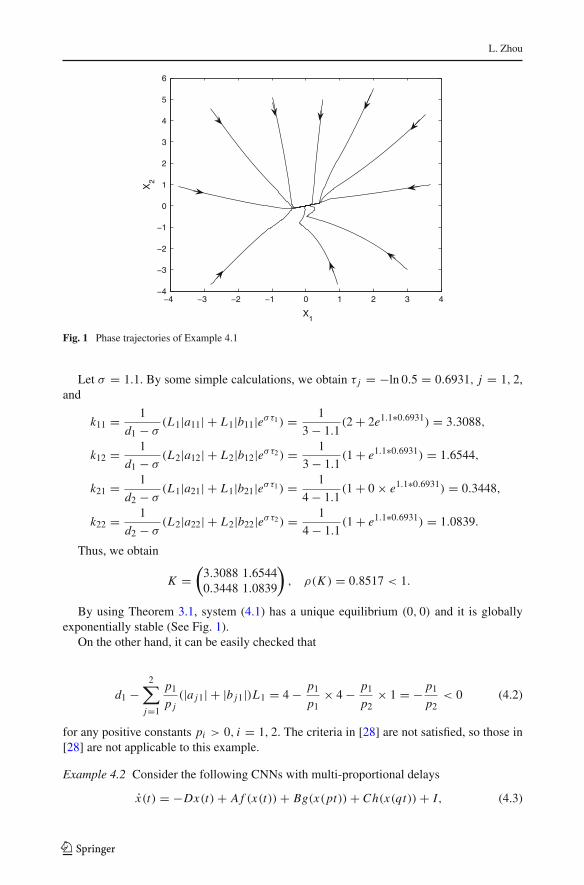
Fig. 1 Phase trajectories of Example 4.1

Let σ = 1.1. By some simple calculations, we obtain τ j = −ln 0.5 = 0.6931, j = 1, 2,and

k11 = 1

d1 − σ(L1|a11| + L1|b11|eστ1) = 1

3 − 1.1(2 + 2e1.1∗0.6931) = 3.3088,

k12 = 1

d1 − σ(L2|a12| + L2|b12|eστ2) = 1

3 − 1.1(1 + e1.1∗0.6931) = 1.6544,

k21 = 1

d2 − σ(L1|a21| + L1|b21|eστ1) = 1

4 − 1.1(1 + 0 × e1.1∗0.6931) = 0.3448,

k22 = 1

d2 − σ(L2|a22| + L2|b22|eστ2) = 1

4 − 1.1(1 + e1.1∗0.6931) = 1.0839.

Thus, we obtain

K =(

3.3088 1.65440.3448 1.0839

)

, ρ(K ) = 0.8517 < 1.

By using Theorem 3.1, system (4.1) has a unique equilibrium (0, 0) and it is globallyexponentially stable (See Fig. 1).

On the other hand, it can be easily checked that

d1 −2∑

j=1

p1

p j(|a j1| + |b j1|)L1 = 4 − p1

p1× 4 − p1

p2× 1 = − p1

p2< 0 (4.2)

for any positive constants pi > 0, i = 1, 2. The criteria in [28] are not satisfied, so those in[28] are not applicable to this example.

Example 4.2 Consider the following CNNs with multi-proportional delays

x(t) = −Dx(t) + A f (x(t)) + Bg(x(pt)) + Ch(x(qt)) + I, (4.3)

123

Delay-Dependent Exponential Stability of Cellular Neural Networks

−10−5

05

10

−10

−5

0

5

10−10

−5

0

5

10

X1

X2

X3

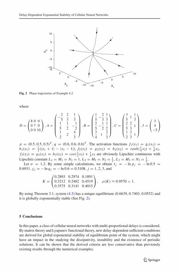
Fig. 2 Phase trajectories of Example 4.2

where

D =⎛

⎝8 0 00 7 00 0 10

⎞

⎠ , A =

⎛

⎜⎜⎜⎜⎜⎝

−2

5

2

3

1

31

5

1

2−1

21

22

4

3

⎞

⎟⎟⎟⎟⎟⎠

, B =

⎛

⎜⎜⎜⎜⎜⎝

1

5−2

3

1

32

5−1

2

1

23

41

2

3

⎞

⎟⎟⎟⎟⎟⎠

, C =

⎛

⎜⎜⎜⎜⎜⎝

3

51

1

32

5

2

31

1

2

2

31

⎞

⎟⎟⎟⎟⎟⎠

, I =⎛

⎝34

−5

⎞

⎠

p = (0.5, 0.5, 0.5)T , q = (0.6, 0.6, 0.6)T . The activation functions f1(x1) = g1(x1) =h1(x1) = 1

2 (|x1 + 1| − |x1 − 1|), f2(x2) = g2(x2) = h2(x2) = tanh( 14 x2) + 1

4 x2,

f3(x3) = g3(x3) = h3(x3) = cos( 12 x3) + 1

4 x3 are obviously Lipschitz continuous withLipschitz constant L1 = M1 = N1 = 1, L2 = M2 = N2 = 1

2 , L3 = M3 = N3 = 34 .

Let σ = 1.2. By some simple calculations, we obtain τ j = − ln p j = − ln 0.5 =0.6931, ς j = − ln q j = − ln 0.6 = 0.5108, j = 1, 2, 3, and

K =⎛

⎝0.2893 0.2974 0.18910.3212 0.2482 0.45190.3575 0.3141 0.4015

⎞

⎠ , ρ(K ) ≈ 0.9570 < 1.

By using Theorem 3.1, system (4.3) has a unique equilibrium (0.6639, 0.7403, 0.0552) andit is globally exponentially stable (See Fig. 2).

5 Conclusions

In this paper, a class of cellular neural networks with multi-proportional delays is considered.By matrix theory and Lyapunov functional theory, new delay-dependent sufficient conditionsare derived for global exponential stability of equilibrium point of the system, which mighthave an impact in the studying the dissipativity, instability and the existence of periodicsolutions. It can be shown that the derived criteria are less conservative than previouslyexisting results through the numerical examples.

123

L. Zhou

Acknowledgements The author would like to thank the Editor and the anonymous reviewers for their valu-able comments and constructive suggestions. The project is supported by the National Science Foundation ofChina (No.60974144), Tianjin Municipal Education commission (No.20100813) and Foundation for Doctorsof Tianjin Normal University (No.52LX34).

References

1. Kato T, Mcleod JB (1971) The functional-differential equation. Bull Am Math Soc 77(2):891–9372. Fox L, Mayers DF (1971) On a functional differential equational. J Inst Math Appl 8(3):271–3073. Iserles A (1994) The asymptotic behavior of certain difference equation with proportional delays. Comput

Math Appl 28(1–3):141–1524. Iserles A (1997) On neural functional-differential equation with proportional delays. J Math Anal Appl

207(1):73–955. Liu YK (1996) Asymptotic behavior of functional differential equations with proportional time delays.

Eur J Appl Math 7(1):11–306. Van B, Marshall JC, Wake GC (2004) Holomorphic solutions to pantograph type equations with neural

fixed points. J Math Anal Appl 295(2):557–5697. Tan MC (2006) Feedback stabilibzation of linear systems with proportional delay. Inf Control (China)

35(6):690–6948. Wang Ch, Kao YG, Yang GW (2012) Exponential stability of impulsive stochastic fuzzy reaction-diffusion

Cohen-Grossberg neural networks with mixed delays. Neurocomputing 89:55–639. Kao YG, Wang JF, Wang Ch, Sun XQ (2012) Delay-dependent robust exponential stability of Markov-

ian jumping reaction- diffusion Cohen-Grossberg neural networks with mixed delays. J Franklin Inst349(6):1972–1988

10. Li T, Guo L, Sun CY, Lin C (2008) Further results on delay-dependent stability criteria of neural networkswith time-varying delays. IEEE Trans Neural Networks 19(4):726–730

11. Roska T, Chua LO (1992) Cellular neural networks with delay type template elements and nonuniformgrids. Int J Circuit Theory Appl 20(4):469–481

12. Tan MC (2010) Global Asympotic stability of fuzzy cellular neural networks with unbounded distributeddelays. Neural Process Lett 31(2):147–157

13. Zhang Q, Wei XP, Xu J (2005) Delay-depend exponential stability of cellular neural networks withtime-varying delays. Appl Math Comput 195(2):402–411

14. Singh V (2007) On global exponential stability of delayed cellular neural networks. Chaos SolitonsFractals 33(1):188–193

15. Balasubramaniam P, Syedali M, Arik S (2010) Global asymptotic stability of stochastic fuzzy cellularneural networks with multi time-varying delays. Expert Syst Appl 37(12):7737–7744

16. Fang Z, Lam J (2011) Stability and dissipativity analysis of distributed delay cellular neural networks.IEEE Trans Neural Networks 22(6):981–997

17. Kao Y, Gao C (2008) Global exponential stability analysis for cellular neural networks with variablecoffciants and delays. Neural Comput Appl 17(3):291–296

18. Liao X, Wang J, Zeng Z (2005) Global asymptotic stability and global exponential stability of delayedcellular neural networks. IEEE trans Circuits Syst-II 52(7):403–409

19. Hu L, Gao H, Zheng W (2009) Novel stability of cellular neural networks with interval time-varyingdelay. Neural Networks 21(10):1458–1463

20. Huang C, Cao J (2009) Almost sure exponential stability of stochastic cellular neural networks withunbounded distributed delays. Neurcomputing 72(13–15):3352–3356

21. Li L, Huang L (2010) Equilibrium analysis for improved signal range model of delayed cellular neuralnetworks. Neural Process Lett 31(3):1771–1794

22. Gan Q, Xu U, Yang P (2010) Stability analysis of stochastic fuzzy cellular neural networks with time-varying delays and reaction-difffusion terms. Neural Process Lett 32:45–57

23. Balasubramaniam P, Vembarasan V, Rakkiyappan R (2011) Leakage delays in T-S fuzzy cellular neuralnetworks. Neural Process Lett 33(2):111–136

24. Balasubramaniam P, Kalpana M, Rakkiyappan R (2011) Global asymptotic stability of BAM fuzzy cellularneural networks with time delay in the leakage term, discrete and unbounded distributed delays. MathComput Model 53(5–6):839–853

25. He HL, Yan L, Tu JJ (2012) Guaranteed cost stabilization of time-varying delay cellular neural networksvia Riccati inequality approach. Neural Process Lett 35(2):151–158

123

Delay-Dependent Exponential Stability of Cellular Neural Networks

26. Tu JJ, He HL (2012) Guaranteed cost synchronization of chaotic cellular neural networks with time-varying delay. Neural Comput 24(1):217–233

27. Zhou L (2011) On the global dissipativity of a class of cellular neural networks with multipantographdelays. Adv Artif Neural Syst 2011:941426

28. Zhang Y, Zhou L (2012) Exponential stability of a class of cellular neural networks with multi-pantographdelays. Acta Electronica Sinica (China) 40(6):1159–1163

29. LaSalle JP (1976) The stability of dynamical system. SIAM, Philadelphia30. Berman A, Plemmons RJ (1979) Nonnegative mathrices in the mathematical science. Academic Presss,

New York

123