On the “Degrees of Freedom” of the Lasso

Hui Zou∗

Trevor Hastie†

Robert Tibshirani‡

Abstract

We study the degrees of freedom of the Lasso in the framework of Stein’s unbiasedrisk estimation (SURE). We show that the number of non-zero coefficients is an unbi-ased estimate for the degrees of freedom of the Lasso—a conclusion that requires nospecial assumption on the predictors. Our analysis also provides mathematical supportfor a related conjecture by Efron et al. (2004). As an application, various model selec-tion criteria—Cp, AIC and BIC—are defined, which, along with the LARS algorithm,provide a principled and efficient approach to obtaining the optimal Lasso fit withthe computational efforts of a single ordinary least-squares fit. We propose the use ofBIC-Lasso shrinkage if the Lasso is primarily used as a variable selection method.

∗Department of Statistics, Stanford University, Stanford, CA 94305. Email: hzou@stanford.edu.†Department of Statistics and Department of Health Research & Policy, Stanford University, Stanford,

CA 94305. Email: hastie@stanford.edu.‡Department of Health Research & Policy and Department of Statistics, Stanford University, Stanford,

CA 94305. Email: tibs@stanford.edu.

1

1 Introduction

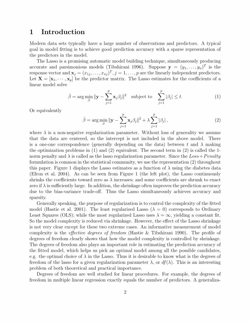
Modern data sets typically have a large number of observations and predictors. A typicalgoal in model fitting is to achieve good prediction accuracy with a sparse representation ofthe predictors in the model.

The Lasso is a promising automatic model building technique, simultaneously producingaccurate and parsimonious models (Tibshirani 1996). Suppose y = (y1, . . . , yn)T is theresponse vector and xj = (x1j, . . . , xnj)

T , j = 1, . . . , p are the linearly independent predictors.Let X = [x1, · · · ,xp] be the predictor matrix. The Lasso estimates for the coefficients of alinear model solve

β = arg minβ‖y −

p∑

j=1

xjβj‖2 subject to

p∑

j=1

|βj| ≤ t. (1)

Or equivalently

β = arg minβ‖y −

p∑

j=1

xjβj‖2 + λ

p∑

j=1

|βj| , (2)

where λ is a non-negative regularization parameter. Without loss of generality we assumethat the data are centered, so the intercept is not included in the above model. Thereis a one-one correspondence (generally depending on the data) between t and λ makingthe optimization problems in (1) and (2) equivalent. The second term in (2) is called the 1-norm penalty and λ is called as the lasso regularization parameter. Since the Loss+Penaltyformulation is common in the statistical community, we use the representation (2) throughoutthis paper. Figure 1 displays the Lasso estimates as a function of λ using the diabetes data(Efron et al. 2004). As can be seen from Figure 1 (the left plot), the Lasso continuouslyshrinks the coefficients toward zero as λ increases; and some coefficients are shrunk to exactzero if λ is sufficiently large. In addition, the shrinkage often improves the prediction accuracydue to the bias-variance trade-off. Thus the Lasso simultaneously achieves accuracy andsparsity.

Generally speaking, the purpose of regularization is to control the complexity of the fittedmodel (Hastie et al. 2001). The least regularized Lasso (λ = 0) corresponds to OrdinaryLeast Squares (OLS); while the most regularized Lasso uses λ =∞, yielding a constant fit.So the model complexity is reduced via shrinkage. However, the effect of the Lasso shrinkageis not very clear except for these two extreme cases. An informative measurement of modelcomplexity is the effective degrees of freedom (Hastie & Tibshirani 1990). The profile ofdegrees of freedom clearly shows that how the model complexity is controlled by shrinkage.The degrees of freedom also plays an important role in estimating the prediction accuracy ofthe fitted model, which helps us pick an optimal model among all the possible candidates,e.g. the optimal choice of λ in the Lasso. Thus it is desirable to know what is the degrees offreedom of the lasso for a given regularization parameter λ, or df(λ). This is an interestingproblem of both theoretical and practical importance.

Degrees of freedom are well studied for linear procedures. For example, the degrees offreedom in multiple linear regression exactly equals the number of predictors. A generaliza-

2

0 2 4 6

−50

00

500

1

2

3

4

5

6

7

8

9

10

PSfrag replacements

Lasso as a shrinkage method

log(1 + λ)

Sta

nd

ard

ized

Coeffi

cien

ts

df(λ)Unbiased estimate for df(λ)

0 2 4 6

24

68

10

PSfrag replacements

Lasso as a shrinkage method

log(1 + λ)Standardized Coefficients

df(λ

)

Unbiased estimate for df(λ)

Figure 1: Diabetes data with 10 predictors. The left panel shows the Lasso coefficients estimatesβj , j = 1, 2, . . . , 10, for the diabetes study. The diabetes data were standardized. The Lasso coeffi-cients estimates are piece-wise linear functions of λ (Efron et al. 2004), hence they are piece-wisenon-linear as functions of log(1 + λ). The right panel shows the curve of the proposed unbiasedestimate for the degrees of freedom of the Lasso, whose piece-wise constant property is basicallydetermined by the piece-wise linearity of β.

3

tion is made for all linear smoothers (Hastie & Tibshirani 1990), where the fitted vector iswritten as y = Sy and the smoother matrix S is free of y. Then df(S) = tr(S) (see Section 2).A leading example is ridge regression (Hoerl & Kennard 1988) with S = (XTX+λI)−1XTX.These results rely on the convenient expressions for representing linear smoothers. Unfor-tunately, the explicit expression of the Lasso fit is not available (at least so far) due to thenonlinear nature of the Lasso, thus the nice results for linear smoothers are not directlyapplicable.

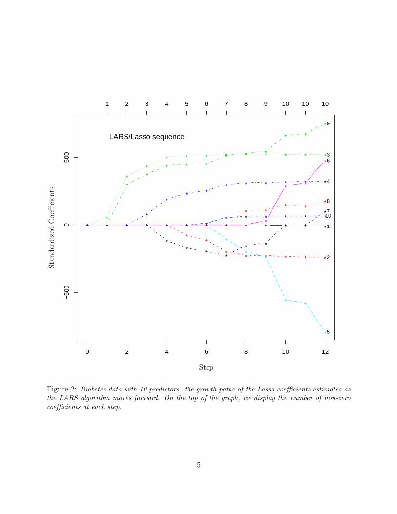
Efron et al. (2004) (referred to as the LAR paper henceforth) propose Least Angle Re-gression (LARS), a new stage-wise model building algorithm. They show that a simplemodification of LARS yields the entire Lasso solution path with the computational cost ofa single OLS fit. LARS describes the Lasso as a forward stage-wise model fitting process.Starting at zero, the Lasso fits are sequentially updated till reaching the OLS fit, while be-ing piece-wise linear between successive steps. The updates follow the current equiangulardirection. Figure 2 shows how the Lasso estimates evolve step by step.

From the forward stage-wise point of view, it is natural to consider the number of stepsas the meta parameter to control the model complexity. In the LAR paper, it is shown thatunder a “positive cone” condition, the degrees of freedom of LARS equals the number ofsteps, i.e., df(µk) = k, where µk is the fit at step k. Since the Lasso and LARS coincideunder the positive cone condition, the remarkable formula also holds for the Lasso. Undergeneral situations df(µk) is still well approximated by k for LARS. However, this simpleapproximation cannot be true in general for the Lasso because the total number of Lassosteps can exceed the number of predictors. This usually happens when some variablesare temporally dropped (coefficients cross zero) during the LARS process, and they areeventually included into the full OLS model. For instance, the LARS algorithm takes 12Lasso steps to reach the OLS fit as shown in Figure 2, but the number of predictors is 10. Forthe degrees of freedom of the Lasso under general conditions, Efron et al. (2004) presentedthe following conjecture.

Conjecture 1 (EHJT04). Starting at step 0, let mk be the index of the last model in theLasso sequence containing k predictors. Then df(µmk)

.= k.

In this paper we study the degrees of freedom of the Lasso using Stein’s unbiased riskestimation (SURE) theory (Stein 1981). The Lasso exhibits the backward penalizationand forward growth pictures, which consequently induces two different ways to describe itsdegrees of freedom. With the representation (2), we show that for any given λ the number ofnon-zero predictors in the model is an unbiased estimate for the degrees of freedom, and nospecial assumption on the predictors is required, e.g. the positive cone condition. The rightpanel in Figure 1 displays the unbiased estimate for the degrees of freedom as a functionof λ on diabetes data (with 10 predictors). If the Lasso is viewed as a forward stage-wiseprocess, our analysis provides mathematical support for the above conjecture.

The rest of the paper is organized as follows. We first briefly review the SURE theory inSection 2. Main results and proofs are presented in Section 3. In Section 4, model selectioncriteria are constructed using the degrees of freedom to adaptively select the optimal Lassofit. We address the difference between two types of optimality: adaptive in prediction and

4

* * * * * * * * * * * * *

0 2 4 6 8 10 12

−50

00

500

* * * * *

**

** * * * *

**

*

*

* * * * * * * * *

* * *

*

** *

* * * * * *

* * * * * * *

*

**

* *

*

* * * * * * * * **

**

*

* * * *

** *

*

* *

* *

*

* * * * * * * *

* ** *

*

* *

*

** * *

* * *

* *

*

* * * * * * ** * * * * *

1

2

3

4

5

6

7

8

9

10

1 2 3 4 5 6 7 8 9 10 10 10

LARS/Lasso sequence

PS

fragrep

lacemen

ts

Lasso

asa

forward

stage-wise

mod

eling

algorithm

Sta

nd

ard

ized

Coeffi

cien

ts

Step

Figure 2: Diabetes data with 10 predictors: the growth paths of the Lasso coefficients estimates asthe LARS algorithm moves forward. On the top of the graph, we display the number of non-zerocoefficients at each step.

5

adaptive in variable selection. Discussions are in Section 5. Proofs of lemmas are presentedin the appendix.

2 Stein’s Unbiased Risk Estimation

We begin with a brief introduction to the Stein’s unbiased risk estimation (SURE) theory(Stein 1981) which is the foundation of our analysis. The readers are referred to Efron (2004)for detailed discussions and recent references on SURE.

Given a model fitting method δ, let µ = δ(y) represent its fit. We assume a homoskedasticmodel, i.e., given the x’s, y is generated according to

y ∼ (µ, σ2I), (3)

where µ is the true mean vector and σ2 is the common variance. The focus is how accurate δcan be in predicting future data. Suppose ynew is a new response vector generated from (3),

then under the squared-error loss, the prediction risk is E{‖µ − ynew‖2

}/n. Efron (2004)

shows that

E{‖µ− µ‖2} = E{‖y − µ‖2 − nσ2}+ 2n∑

i=1

cov(µi, yi). (4)

The last term of (4) is called the optimism of the estimator µ (Efron 1986). Identity (4) alsogives a natural definition of the degrees of freedom for an estimator µ = δ(y),

df(µ) =n∑

i=1

cov(µi, yi)/σ2. (5)

If δ is a linear smoother, i.e., µ = Sy for some matrix S independent of y, then it is easy toverify that since cov(µ,y) = σ2S, df(µ) = tr(S), which coincides with the definition givenby Hastie & Tibshirani (1990). By (4) we obtain

E{‖µ− ynew‖2} = E{‖y − µ‖2 + 2df(µ) σ2}. (6)

Thus we can define a Cp-type statistic

Cp(µ) =‖y − µ‖2

n+

2df(µ)

nσ2 (7)

which is an unbiased estimator of the true prediction error. When σ2 is unknown, it isreplaced with an unbiased estimate.

Stein proves an extremely useful formula to simplify (5), which is often referred to asStein’s Lemma (Stein 1981). According to Stein, a function g : Rn → R is said to be almostdifferentiable if there is a function f : Rn → Rn such that

g(x+ u)− g(x) =

∫ 1

0

uTf(x+ tu)dt (8)

for a.e. x ∈ Rn, each u ∈ Rn.

6

Lemma 1 (Stein’s Lemma). Suppose that µ : Rn → Rn is almost differentiable and denote∇ · µ =

∑ni=1 ∂µi/∂yi. If y ∼ Nn(µ, σ2I), then

n∑

i=1

cov(µi, yi)/σ2 = E[∇ · µ]. (9)

In many applications ∇ · µ is shown to be a constant; for example, with µ = Sy,∇ · µ = tr(S). Thus the degrees of freedom is easily obtained. Even if ∇ · µ depends on y,Stein’s Lemma says

df(µ) = ∇ · µ (10)

is an unbiased estimate for the degrees of freedom df(µ). In the spirit of SURE, we can use

C∗p(µ) =‖y − µ‖2

n+

2df(µ)

nσ2 (11)

as an unbiased estimate for the true risk. It is worth mentioning that in some situationsverifying the almost differentiability of µ is not easy.

Even though Stein’s Lemma assumes normality, the essence of (9) only requires ho-moskedasticity (3) and the almost differentiability of µ; its justification can be made by a“delta method” argument (Efron et al. 2004). After all, df(µ) is about the self-influenceof y on the fit, and ∇ · µ is a natural candidate for that purpose. Meyer & Woodroofe(2000) discussed the degrees of freedom in shape-restricted regression and argued that thedivergence formula (10) provides a measure of the effective dimension.

3 Main Theorems

We adopt the SURE framework with the Lasso fit. Let µλ be the Lasso fit using therepresentation (2). Similarly, let µm be the Lasso fit at step m in the LARS algorithm. Forconvenience, we also let df(λ) and df(m) stand for df(µλ) and df(µm), respectively.

The following matrix representation of Stein’s Lemma is helpful. Let ∂µ∂y

be a n × nmatrix whose elements are

(∂µ

∂y

)

i,j

=∂µi∂yj

i, j = 1, 2, . . . , n. (12)

Then we can write

∇ · µ = tr

(∂µ

∂y

). (13)

Suppose M is a matrix with p columns. Let S be a subset of the indices {1, 2, . . . , p}.Denote by MS the sub-matrix

MS = [· · ·mj · · · ]j∈S , (14)

7

where mj is the j-th column of M. Similarly, define βS = (· · · βj · · · )j∈S for any vector β oflength p. Let Sgn(·) be the sign function:

Sgn(x) =

1 if x > 0

0 if x = 0

−1 if x < 0

3.1 Results and data examples

Our results are stated as follows. Denote the set of non-zero elements of βλ as B(λ), then

df(λ) = E[|Bλ|] (15)

where |Bλ| means the size of B(λ). Hence df(λ) = |Bλ| is an unbiased estimate for df(λ).The identity (15) holds for all X, requiring no special assumption.

We also provide mathematical support for the conjecture in Section 1. Actually we arguethat if mk is a Lasso step containing k non-zero predictors, then df(mk) = k is a goodestimate for df(mk). Note that mk is not necessary the last Lasso step containing k non-zeropredictors. So the result includes the conjecture as a special case. However, we show inSection 4 that the last step choice is superior in the Lasso model selection. We let mlast

k andmfirstk denote the last and first Lasso step containing exact k non-zero predictors, respectively.

Before delving into the detail of theoretical analysis, we check the validity of our argu-ments by a simulation study. Here is the outline of the simulation. We take the 64 predictorsin the diabetes data which include the quadratic terms and interactions of the original 10predictors. The positive cone condition is violated on the 64 predictors (Efron et al. 2004).The response vector y was used to fit a OLS model. We computed the OLS estimates βolsand σ2

ols. Then we considered a synthetic model

y∗ = Xβ +N(0, 1)σ, (16)

where β = βols and σ = σols.Given the synthetic model, the degrees of freedom of the Lasso (both df(λ) and df(mk))

can be numerically evaluated by Monte Carlo methods. For b = 1, 2, . . . , B, we independentlysimulated y∗(b) from (16). For a given λ, by the definition of df(λ), we need to evaluate

covi = E[(µλ,i − E[µλ,i])(y∗i − (Xβ)i)]. (17)

Then df(λ) =∑n

i=1 covi/σ2. Since E[y∗i ] = (Xβ)i and note that

covi = E[(µλ,i − ai)(y∗i − (Xβ)i)] (18)

for any fixed known constant ai. Then we compute

covi =

∑Bb=1

(µλ,i(b)− ai

)(y∗i (b)− (Xβ)i)

B(19)

8

and df(λ) =∑n

i=1 covi/σ2. Typically ai = 0 is used in Monte Carlo calculation. In this work

we use ai = (Xβ)i, for it gives a Monte Carlo estimate for df(λ) with smaller variance thanthat by ai = 0. On the other hand, for a fixed λ, each y∗(b) gave the Lasso fit µλ(b) and the

df estimate df(λ)b. Then we evaluated E[|Bλ|] by∑B

b=1 df(λ)b/B. Similarly, we computeddf(mk) by replacing µλ(b) with µmk(b). We are interested in E[|Bλ|]−df(λ) and k−df(mk).Standard errors were calculated based on the B replications.

Figure 3 is a very convincing picture for the identity (15). Figure 4 shows that df(mk)is well approximated by k even when the positive cone condition is failed. The simpleapproximation works pretty well for both mlast

k and mfirstk .

In Figure 4, it appears that k − df(mk) is not exactly zero for some k. We would like tocheck if the bias is real. Furthermore, if the bias is real, then we would like to explore therelation between the bias k− df(mk) and the signal/noise ratio. In the synthetic model (16)

the signal/noise ratioVar(Xβols)

σ2ols

is about 1.25. We repeated the same simulation procedure

with (β = 0, σ = 1) and (β = βols, σ = σols10

) in the synthetic model. The correspondingsignal/noise ratios are zero and 125, respectively.

As shown clearly in Figure 5, the bias k− df(mk) is truly non-zero for some k. Thus thepositive cone condition seems to be sufficient and necessary for turning the approximationinto an exact result. However, even if the bias exists, its maximum magnitude is less thanone, regardless the size of the signal/noise ratio. So k is a very good estimate for df(mk). Aninteresting observation is that k tends to underestimate df(mlast

k ) and overestimate df(mfirstk ).

In addition, we observe that k − df(mlastk )

.= df(mfirst

k )− k.

3.2 Theorems on df(λ)

Let B = {j : Sgn(β)j 6= 0} be the active set of β where Sgn(β) is the sign vector of β given

by Sgn(β)j = Sgn(βj). We denote the active set of β(λ) as B(λ) and the corresponding sign

vector Sgn(β(λ)) as Sgn(λ). We do not distinguish the index of a predictor and the predictoritself.

Firstly, let us review some characteristics of the Lasso solution. For a given responsevector y, there are a sequence of λ’s:

λ0 > λ1 > λ2 · · · > λK = 0 such that: (20)

• For all λ > λ0, β(λ) = 0.

• In the interior of the interval (λm+1, λm), the active set B(λ) and the sign vectorSgn(λ)B(λ) are constant with respect to λ. Thus we write them as Bm and Sgnm forconvenience.

The active set changes at each λm. When λ decreases from λ = λm − 0, some predictorswith zero coefficients at λm are about to have non-zero coefficients, thus they join the activeset Bm. However, as λ approaches λm+1 + 0 there are possibly some predictors in Bm whosecoefficients reach zero. Hence we call {λm} the transition points.

We shall proceed by proving the following lemmas (proofs are given in the appendix).

9

0 10 20 30 40 50 60

010

2030

4050

60

PS

fragrep

lacemen

ts

dfco

mp

ute

dby

Mon

teC

arlo

E[|Bλ|]

df(λ)

E[|B

λ |−df

(λ)]

0 10 20 30 40 50 60

−1.

0−

0.5

0.0

0.5

1.0

PS

fragrep

lacemen

ts

dfcom

pu

tedby

Mon

teC

arlo

E[|Bλ|]

df(λ)

E[|B

λ|−

df(λ

)]Figure 3: The synthetic model with the 64 predictors in the diabetes data. In the left panel wecompare E[|Bλ|] with the true degrees of freedom df(λ) based on B = 20000 Monte Carlo simula-tions. The solid line is the 450 line (the perfect match). The right panel shows the estimation biasand its point-wise 95% confidence intervals indicated by the thin dashed lines. Note that the zerohorizontal line is well inside the confidence intervals.

0 10 20 30 40 50 60

010

2030

4050

60

PS

fragrep

lacemen

ts

dfco

mp

ute

dby

Mon

teC

arlo

The last step containing k variables

Th

efi

rststep

contain

ingk

variables

k

0 10 20 30 40 50 60

010

2030

4050

60

PS

fragrep

lacemen

ts

dfco

mp

ute

dby

Mon

teC

arlo

Th

elast

stepcon

tainin

gk

variables

The first step containing k variables

k

Figure 4: The synthetic model with the 64 predictors in the diabetes data. We compare df(mk)with the true degrees of freedom df(mk) based on B = 20000 Monte Carlo simulations. We considertwo choices of mk: in the left panel mk is the last Lasso step containing exact k non-zero variables,while the right panel chooses the first Lasso step containing exact k non-zero variables. As can beseen from the plots, our formula works pretty well in both cases.

10

−1.

0−

0.5

0.0

0.5

1.0

signal/noise=1.25

obj$k

obj$

k −

obj

$df.f

irst

signal/noise=1.25

obj$k

obj$

k −

obj

$df.l

ast

−1.

0−

0.5

0.0

0.5

1.0

signal/noise=0

obj$k

obj$

k −

obj

$df.f

irst

signal/noise=0

obj$k

obj$

k −

obj

$df.l

ast

signal/noise=125

−1.

0−

0.5

0.0

0.5

1.0

0 10 20 30 40 50 60

obj$k

obj$

k −

obj

$df.f

irst

0 10 20 30 40 50 60

signal/noise=125

PSfrag replacements

k−df

(mk)

k−df

(mk)

k−df

(mk)

The last step mlastk The first step mfirst

k

kk

Figure 5: B = 20000 replications were used to assess the bias of df(mk) = k. The 95% point-wiseconfidence intervals are indicated by the thin dashed lines. Under the positive cone condition, it isexactly the true degrees of freedom df(mk). This simulation suggests that when the positive conecondition is violated, df(mk) 6= k for some k. However, the bias is small (the maximum absolutebias is about 0.8). It seems that k tends to underestimate df(mlast

k ) and overestimate df(mfirstk ). In

addition, we observe that k − df(mlastk )

.= df(mfirst

k ) − k. The most important message is that themagnitude of the bias is always less than one, regardless the size of the signal/noise ratio.

11

Lemma 2. Suppose λ ∈ (λm+1, λm). β(λ) are the Lasso coefficient estimates. Then we have

β(λ)Bm =(XTBmXBm

)−1(

XTBmy − λ

2Sgnm

). (21)

Lemma 3. Consider the transition points λm and λm+1, λm+1 ≥ 0. Bm is the active set in(λm+1, λm). Suppose iadd is an index added into Bm at λm and its index in Bm is i∗, i.e.,iadd = (Bm)i∗. Denote by (a)k the k-th element of the vector a. We can express the transitionpoint λm as follows:

λm =2((

XTBmXBm

)−1XTBmy

)i∗((

XTBmXBm

)−1Sgnm

)i∗

(22)

Moreover, if jdrop is a dropped (if there is any) index at λm+1 and jdrop = (Bm)j∗, then λm+1

can be written as:

λm+1 =2((

XTBmXBm

)−1XTBmy

)j∗((

XTBmXBm

)−1Sgnm

)j∗

(23)

Lemma 4. ∀ λ > 0, ∃ a null set Nλ which is a finite collection of hyperplanes in Rn. LetGλ = Rn \ Nλ. Then ∀y ∈ Gλ, λ is not any of the transition points, i.e., λ /∈ {λ(y)m}.

Lemma 5. ∀λ, βλ(y) is a continuous function of y.

Lemma 6. Fix any λ > 0, consider y ∈ Gλ as defined in Lemma 4. The active set B(λ)and the sign vector Sgn(λ) are locally constant with respect to y.

Theorem 1. Let G0 = Rn. Fix an arbitrary λ ≥ 0. On the set Gλ with full measure asdefined in Lemma 4, the Lasso fit µλ(y) is uniformly Lipschitz. Precisely,

‖µλ(y + ∆y)− µλ(y)‖ ≤ ‖∆y‖ for sufficiently small ∆y (24)

Moreover, we have the divergence formula

∇ · µλ(y) = |Bλ|. (25)

Proof. If λ = 0, then the Lasso fit is just the OLS fit. The conclusions are easy to verify. Sowe focus on λ > 0. Fix a y. Choose a small enough ε such that Ball(y, ε) ⊂ Gλ.

Since λ is not any transition point, using (21) we observe

µλ(y) = Xβ(y) = Hλ(y)y − λωλ(y), (26)

where Hλ(y) = XBλ(XTBλXBλ)−1XT

Bλ is the projection matrix on the space XBλ and ωλ(y) =12

XBλ(XTBλXBλ)−1SgnBλ . Consider ‖∆y‖ < ε. Similarly, we get

µλ(y + ∆y) = Hλ(y + ∆y)(y + ∆y)− λωλ(y + ∆y). (27)

12

Lemma 6 says that we can further let ε be sufficiently small such that both the effectiveset Bλ and the sign vector Sgnλ stay constant in Ball(y, ε). Now fix ε. Hence if ‖∆y‖ < ε,then

Hλ(y + ∆y) = Hλ(y) and ωλ(y + ∆y) = ωλ(y). (28)

Then (26) and (27) giveµλ(y + ∆y)− µλ(y) = Hλ(y)∆y. (29)

But since ‖Hλ(y)∆y‖ ≤ ‖∆y‖, (24) is proved.By the local constancy of H(y) and ω(y), we have

∂µλ(y)

∂y= Hλ(y). (30)

Then the trace formula (13) implies

∇ · µλ(y) = tr (Hλ(y)) = |Bλ|. (31)

By standard analysis arguments, it is easy to check the following propositionProposition Let f : Rn → Rn and suppose f is uniformly Lipschitz on G = Rn \ N whereN is a finite set of hyperplanes. If f is continuous, then f is uniformly Lipschitz on Rn.

Theorem 2. ∀ λ the Lasso fit µλ(y) is uniformly Lipschitz. The degrees of freedom of µλ(y)equal the expectation of the effective set Bλ, i.e.,

df(λ) = E [|Bλ|] . (32)

Proof. The proof is trivial for λ = 0. We only consider λ > 0. By Theorem 1 and theproposition, we conclude that µλ(y) is uniformly Lipschitz. Therefore µλ(y) is almostdifferentiable, see Meyer & Woodroofe (2000) and Efron et al. (2004). Then (32) is obtainedby Stein’s Lemma and the divergence formula (25).

3.3 df(mk) and the conjecture

In this section we provide mathematical support for the conjecture in Section 1. The con-jecture becomes a simple fact for two trivial cases k = 0 and k = p, thus we only need toconsider k = 1, . . . , (p− 1). Our arguments rely on the details of the LARS algorithm. Forthe sake of clarity, we first briefly describe the LARS algorithm. The readers are referred tothe LAR paper (Efron et al. 2004) for the complete description.

The LARS algorithm sequentially updates the Lasso estimate in a predictable way. Ini-tially (the 0 step), let β0 = 0, A0 = ∅. Suppose that βm is the vector of current Lassocoefficient estimates. Then µm = Xβm and rm = y − µm are the current fit and residualvectors. We say c = XT rm is the vector of current correlations. Define

C = maxj{|c|} Wm = {j : |cj| = C and j ∈ Acm}. (33)

13

Then λm = 2C. Define the current active set A = Am ∪Wm and the signed matrix

XsignA = (· · · Sgn(cj)xj · · · )j∈A. (34)

Let GA =(XsignA

)TXsignA . 1A is a vector of 1’s of length |A|. Then we compute the equian-

gular vectoruA = Xsign

A wA with wA = DG−1A 1A, (35)

where D = (1TAG−1A 1A)−

12 . Let the inner product vector a = XTuA and

γ = min+j∈Ac

{C − cjD − aj

,C + cjD + aj

}. (36)

For j ∈ A we compute dj = Sgn(cj)wAj and γj = −(βm)j/dj. Define

γ = minγj>0{γj} and Vm = {j : γj = γ j ∈ A}. (37)

The Lasso coefficient estimates are updated by

(βm+1)j = (βm)j + min{γ, γ}dj for j ∈ A. (38)

The set Am is also updated. If γ < γ then Am+1 = A. Otherwise Am+1 = A\Vm.Let qm be the indicator of whether Vm is dropped or not. Define qmVm = Vm if qm = 1,

otherwise qmVm = ∅; and conventionally let V−1 = ∅ and q−1V−1 = ∅. Considering theactive set Bλ as a function of λ, we summarize the following facts

|Bλ| = |Bλm |+ |Wm| if λm < λ < λm+1, (39)

|Bλm+1 | = |Bλm |+ |Wm| − |qmVm|. (40)

In the LARS algorithm, the Lasso is regarded as one kind of forward stage-wise methodfor which the number of steps is often used as an effective regularization parameter. Foreach k, k ∈ {1, 2, . . . , (p− 1)}, we seek the models with k non-zero predictors. Let

Λk = {m : |Bλm | = k}. (41)

The conjecture is asking for the fit using mlastk = sup(Λk). However, it may happen that for

some k there is no such m with |Bλm | = k. For example, if y is an equiangular vector of all{Xj}, then the Lasso estimates become the OLS estimates after just one step. So Λk = ∅for k = 2, . . . , (p− 1). The next Lemma concerns this type of situation. Basically, it showsthat the “one at a time” condition (Efron et al. 2004) holds almost everywhere, thereforeΛk is not empty for all k a.s.

Lemma 7. ∃ a set N0 which is a collection of finite many hyperplanes in Rn. ∀y ∈ Rn \ N0,

|Wm(y)| = 1 and |qmVm(y)| ≤ 1 ∀ m = 0, 1, . . . , K(y). (42)

14

Corollary 1. ∀ y ∈ Rn \ N0, Λk is not empty for all k, k = 0, 1, . . . , p.

Proof. This is a direct consequence of Lemma 7 and (39), (40).

The next theorem presents an expression for the Lasso fit at each transition point, whichhelps us compute the divergence of µmk(y).

Theorem 3. Let µm(y) be the Lasso fit at the transition point λm, λm > 0. Then for anyi ∈ Wm, we can write µ(m) as follows

µm(y) =

{HB(λm) −

XTB(λm)

(XTB(λm)XB(λm)

)Sgn(λm)xTi (I−HB(λm))

Sgni − xTi XTB(λm)

(XTB(λm)XB(λm)

)Sgn(λm)

}y (43)

=: Sm(y)y (44)

where HB(λm) is the projection matrix on the subspace of XB(λm). Moreover

tr (Sm(y)) = |B(λm)|. (45)

Proof. Note that β(λ) is continuous on λ. Using (18) in Lemma 2 and taking the limit ofλ→ λm, we have

−2xTj

(y −

p∑

j=1

xjβ(λm)j

)+ λm Sgn(β(λm)j) = 0, for j ∈ B(λm). (46)

However,∑p

j=1 xjβ(λm)j =∑

j∈B(λm) xjβ(λm)j. Thus we have

β(λm) =(XTB(λm)XB(λm)

)−1(

XTB(λm)y −

λm2

Sgn(λm)

). (47)

Hence

µm(y) = XB(λm)

(XTB(λm)XB(λm)

)−1(

XTB(λm)y −

λm2

Sgn(λm)

)

= HB(λm)y −XB(λm)

(XTB(λm)XB(λm)

)−1Sgn(λm)

λm2. (48)

Since i ∈ Wm, we must have the equiangular condition

Sgni xTi (y − µ(m)) =λm2. (49)

Substituting (48) into (49), we solve λm2

and obtain

λm2

=xTi(I−HB(λm)

)y

Sgni − xTi XTB(λm)

(XTB(λm)XB(λm)

)Sgn(λm)

. (50)

15

Then putting (50) back to (48) yields (43).Using the identity tr(AB) = tr(BA), we observe

tr(Sm(y)−HB(λm)

)= tr

XTB(λm)

(XTB(λm)XB(λm)

)Sgn(λm)xTi (I−HB(λm))

Sgni − xTi XTB(λm)

(XTB(λm)XB(λm)

)Sgn(λm)

= tr

(XTB(λm)XB(λm)

)Sgn(λm)xTi (I−HB(λm))X

TB(λm)

Sgni − xTi XTB(λm)

(XTB(λm)XB(λm)

)Sgn(λm)

= tr (0) = 0.

So tr (Sm(y)) = tr(HB(λm)

)= |B(λm)|.

Definition 1. y ∈ Rn \ N0 is said to be a locally stable point for Λk, if ∀ y′ such that‖y′−y‖ ≤ ε(y) for a small enough ε(y), the effective set Bλm(y′) = Bλm(y), for all m ∈ Λk.Let LS(Λk) be the set of all locally stable points for Λk.

Theorem 4. If y ∈ LS(Λk), then we have the divergence formula ∇· µm(y) = k which holdsfor all m ∈ Λk including mk = sup(Λk), the choice in the conjecture.

Proof. The conclusion immediately follows definition 1 and Theorem 3.

Points in LS(Λk) are the majority of Rn. Under the positive cone condition, LS(Λk) is aset of full measure for all k. In fact the positive cone condition implies a stronger conclusion.

Definition 2. y is said to be a strong locally stable point if ∀ y′ such that ‖y′ − y‖ ≤ ε(y)for a small enough ε(y), the effective set Bλm(y′) = Bλm(y), for all m = 0, 1, . . . , K(y).

Lemma 8. Let N1 ={

y : γ(y) = γ(y) for some m,m ∈ {0, 1, . . . , K(y)}}

. ∀ y ∈ the

interior of Rn \ (N0 ∪ N1), y is a strong locally stable point. In particular, the positive cone

condition implies N1 = ∅.

LARS is a discrete procedure by its definition, but the Lasso is a continuous shrinkagemethod. So it also makes sense to talk about fractional Lasso steps in the LARS algorithm,e.g. what is the Lasso fit at 3.5 steps? Under the positive cone condition, we can generalizethe result of Theorem 4 in the LAR paper to the case of non-integer steps.

Corollary 2. Under the positive cone condition df(µs) = s for all real valued s: 0 ≤ s ≤ p.

Proof. Let k ≤ s < k + 1, s = k + r for some r ∈ [0, 1). According to the LARS algorithm,the Lasso fit is linearly interpolated between steps k and k+1. So µs = µk ·(1−r)+ µk+1 ·r.Then by definition (5) and the fact cov is a linear operator, we have

df(µs) = df(µk) · (1− r) + df(µk+1) · r= k · (1− r) + (k + 1) · r = s. (51)

In (51) we have used the positive cone condition and Theorem 4 in the LAR paper.

16

4 Adaptive Lasso Shrinkage

4.1 Model selection criteria

For any regularization method an important issue is to find a good choice of the regularizationparameter such that the corresponding model is optimal according to some criterion, e.g.minimizing the prediction risk. For this purpose, model selection criteria have been proposedin the literature to compare different models. Famous examples are AIC (Akaike 1973) andBIC (Schwartz 1978). Mallows’s Cp (Mallows 1973) is very similar to AIC and a wholeclass of AIC or Cp-type criteria are provided by SURE theory (Stein 1981). In Efron (2004)Cp and SURE are summarized as covariance penalty methods for estimating the predictionerror, and are shown to offer substantially better accuracy than cross-validation and relatednonparametric methods, if one is willing to assume the model is correct.

In the previous section we have derived the degrees of freedom of the Lasso for bothtypes of regularization: λ and mk. Although the exact value of df(λ) is still unknown, ourformula provides a convenient unbiased estimate. In the spirit of SURE theory, the unbiasedestimate for df(λ) suffices to provide an unbiased estimate for the prediction error of µλ. Ifwe choose mk as the regularization parameter, the good approximation df(µmk)

.= k also

well serves the SURE purpose. Therefore an estimate for the prediction error of µ (pe(µ))is

pe(µ) =‖y − µ‖2

n+

2

ndf(µ) σ2, (52)

where df is either df(λ) or df(mk), depending on the type of regularization. When σ2 isunknown, it is usually replaced with an estimate based on the largest model.

Equation (52) equivalently derives AIC for the Lasso

AIC(µ) =‖y − µ‖2

nσ2+

2

ndf(µ). (53)

Selecting the Lasso model by AIC is called AIC-Lasso shrinkage. Following the usual defi-nition of BIC, we propose BIC for the Lasso as follows

BIC(µ) =‖y − µ‖2

nσ2+

log(n)

ndf(µ). (54)

Similarly the Lasso model selection by BIC is called BIC-Lasso shrinkage.AIC and BIC possess different asymptotic optimality. It is well known that if the true

regression function is not in the candidate models, the model selected by AIC asymptoticallyachieves the smallest average squared error among the candidates; and the AIC estimator ofthe regression function converges at the minimax optimal rate whether the true regressionfunction is in the candidate models or not, see Shao (1997), Yang (2003) and referencestherein. On the other hand, BIC is well known for its consistency in selecting the truemodel (Shao 1997). If the true model is in the candidate list, the probability of selecting thetrue model by BIC approaches one as the sample size n → ∞. Considering the case wherethe true underlying model is sparse, BIC-Lasso shrinkage is adaptive in variable selection.

17

n AIC BIC100 0.162 0.451500 0.181 0.6231000 0.193 0.6862000 0.184 0.702

Table 1: The simulation example: the probability of discovering the exact true model by AIC andBIC Lasso shrinkage. The calculation is based on 2000 replications. Compared with AIC-Lassoshrinkage, BIC-Lasso shrinkage has a much higher probability of identifying the ground truth.

n AIC BIC100 5 4500 5 31000 5 32000 5 3

Table 2: The simulation example: the median of the number of non-zero variables selected by AICand BIC Lasso shrinkage based on 2000 replications. One can see that AIC-Lasso shrinkage isconservative in variable selection and BIC-Lasso shrinkage tends to find models with the right size.

However, AIC-Lasso shrinkage tends to include more non-zero predictors than the truth. Theconservative nature of AIC is a familiar result in linear regression. Hence BIC-Lasso shrinkageis more appropriate than AIC-Lasso shrinkage when variable selection is the primary concernin applying the Lasso.

Here we show a simulation example to demonstrate the above argument. We simulatedresponse vectors y from a linear model: y = Xβ + N(0, 1) where β = (3, 1.5, 0, 0, 2, 0, 0, 0).Predictors {xi} are multivariate normal vectors with pairwise correlation cor(i, j) = (0.1)|i−j|

and the variance of each xi is one. For each estimate β, it is said to discover the exact truemodel if {β1, β2, β5} are non-zero and the rest coefficients are all zero. Table 1 shows theprobability of discovering the exact true model using AIC-Lasso shrinkage and BIC-Lassoshrinkage. In this example both AIC and BIC always select the true predictors {1, 2, 5} inall the 2000 replications, but AIC tends to include other variables as real factors as shownin Table 2. In contrast to AIC, BIC has a much lower false positive rate.

One may think of combining the good properties of AIC and BIC into a new criterion.Although this proposal sounds quite reasonable, a surprising result is proved that any modelselection criterion cannot be consistent and optimal in average squared error at the same time(Yang 2003). In other words, any model selection criterion must sacrifice either predictionoptimality or consistency.

18

4.2 Computation

Using either AIC or BIC to find the optimal Lasso model, we are facing an optimizationproblem

λ(optimal) = arg minλ

‖y − µλ‖2

nσ2+wnn

df(λ), (55)

where wn = 2 for AIC and wn = log(n) for BIC. Since the LARS algorithm efficientlysolves the Lasso solution for all λ, finding λ(optimal) is attainable in principle. In fact, weshow that λ(optimal) is one of the transition points, which further facilitates the searchingprocedure.

Theorem 5. To find λ(optimal), we only need to solve

m∗ = arg minm

‖y − µλm‖2

nσ2+wnn

df(λm) (56)

then λ(optimal) = λm∗.

Proof. Let us consider λ ∈ (λm+1, λm). By (21) we have

y − µλ = (I−HBm)y +λ

2XBm(XT

BmXBm)−1Sgnm (57)

‖y − µλ‖2 = yT (I−HBm)y +λ2

4SgnTm(XT

BmXBm)−1Sgnm (58)

where HBm = XBm(XTBmXBm)−1XT

Bm . Thus we can conclude that ‖y − µλ‖2 is strictlyincreasing in the interval (λm+1, λm). Moreover, the Lasso estimates are continuous on λ,hence

‖y − µλm‖2 > ‖y − µλ‖2 > ‖y − µλm+1‖2. (59)

On the other hand, note that df(λ) = |Bm| ∀ λ ∈ (λm+1, λm) and |Bm| ≥ |B(λm+1)|. There-fore the optimal choice of λ in [λm+1, λm) is λm+1, which means λ(optimal) ∈ {λm},m =0, 1, 2, . . . , K.

According to Theorem 5, the optimal Lasso model is immediately selected once the entireLasso solution path is solved by the LARS algorithm, which has the cost of a single leastsquares fit.

If we consider the best Lasso fit in the forward stage-wise modeling picture (like Figure 2),inequality (59) explains the superiority of the choice of mk in the conjecture. Let mk bethe last Lasso step containing k non-zero predictors. Suppose m′k is another Lasso step

containing k non-zero predictors, then df(µ(m′k)) = k = df(µ(mk)). However, m′k < mk

gives ‖y− µmk‖2 < ‖y− µm′k‖2. Then by the Cp statistic, we see that µ(mk) is always more

accurate than µ(m′k), while using the same number of non-zero predictors. Using k as thetuning parameter of the Lasso, we need to find k(optimal) such that

k(optimal) = arg mink

‖y − µmk‖2

nσ2+wnnk. (60)

19

Once λ∗ = λ(optimal) and k∗ = k(optimal) are found, we fix them as the regularizationparameters for fitting the Lasso on future data. Using the fixed k∗ means the fit on futuredata is µmk∗ , while the fit using the fixed λ∗ is µλ∗ . It is easy to see that the selected modelsby (55) and (60) coincide on the training data, i.e., µλ∗ = µmk∗ .

Figure 6 displays the Cp (equivalently AIC) and BIC estimates of risk using the dia-betes data. The models selected by Cp are the same as those selected in the LAR paper.With 10 predictors, Cp and BIC select the same model using 7 non-zero covariates. With64 predictors, Cp selects a model using 15 covariates, while BIC selects a model with 11covariates.

0 2 4 6 8 10 12

010

020

030

040

0

CpBIC

1 2 3 4 5 6 7 8 9 10 10 10

PS

fragrep

lacemen

ts

Cp,

BIC

Step

0 20 40 60 80 100

010

020

030

040

050

0

CpBIC

11 15

PS

fragrep

lacemen

ts

Cp,

BIC

Step

Figure 6: The diabetes data. Cp and BIC estimates of risk with 10 (left) and 64 (right) predictors.In the left panel Cp and BIC select the same model with 7 non-zero coefficients. In the rightpanel, Cp selects a model with 15 non-zero coefficients and BIC selects a model with 11 non-zerocoefficients.

5 Discussion

It is interesting to note that the true degrees of freedom is a strictly decreasing function ofλ, as shown in Figure 7. However, the unbiased estimate df(λ) is not necessarily monotone,although its global trend is monotonically decreasing. The same phenomenon is also shownin the right panel of Figure 1. The non-monotonicity of df(λ) is due to the fact that somevariables can be dropped during the LARS/Lasso process.

An interesting question is that whether there is a smoothed estimate df∗(λ) such that

df∗(λ) is a smooth decreasing function and keeps the unbiased property, i.e.,

df(λ) = E[df∗(λ)] (61)

20

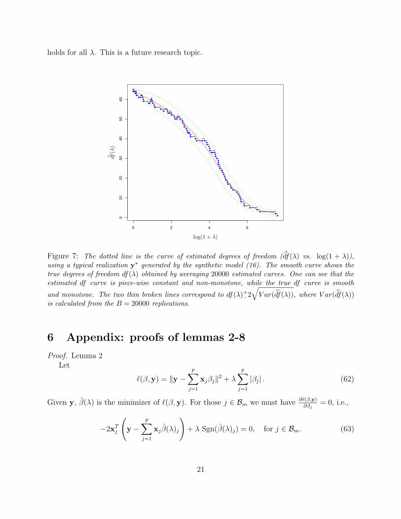
holds for all λ. This is a future research topic.

0 2 4 6

010

2030

4050

60

PS

fragrep

lacemen

ts

df(λ

)

log(1 + λ)

Figure 7: The dotted line is the curve of estimated degrees of freedom (df(λ) vs. log(1 + λ)),using a typical realization y∗ generated by the synthetic model (16). The smooth curve shows thetrue degrees of freedom df(λ) obtained by averaging 20000 estimated curves. One can see that theestimated df curve is piece-wise constant and non-monotone, while the true df curve is smooth

and monotone. The two thin broken lines correspond to df(λ)+−2

√V ar(df(λ)), where V ar(df(λ))

is calculated from the B = 20000 replications.

6 Appendix: proofs of lemmas 2-8

Proof. Lemma 2Let

`(β,y) = ‖y −p∑

j=1

xjβj‖2 + λ

p∑

j=1

|βj| . (62)

Given y, β(λ) is the minimizer of `(β,y). For those j ∈ Bm we must have ∂`(β,y)∂βj

= 0, i.e.,

−2xTj

(y −

p∑

j=1

xjβ(λ)j

)+ λ Sgn(β(λ)j) = 0, for j ∈ Bm. (63)

21

Since β(λ)i = 0 for all i /∈ Bm, then∑p

j=1 xjβ(λ)j =∑

j∈Bλ xjβ(λ)j. Thus equations in (63)become

−2XTBm

(y −XBm β(λ)Bm

)+ λ Sgnm = 0 (64)

which gives (21).

Proof. Lemma 3We adopt the matrix notation used in S : M[i, ] means the i-th row of M. iadd joins Bm

at λm, thenβ(λm)iadd = 0. (65)

Consider β(λ) for λ ∈ (λm+1, λm). Lemma 2 gives

β(λ)Bm =(XTBmXBm

)−1(

XTBmy − λ

2Sgnm

). (66)

By the continuity of β(λ)iadd , taking the limit of the i∗-th element of (66) as λ→ λm− 0, wehave

2

{(XTBmXBm

)−1[i∗, ]XT

Bm

}y = λm

{(XTBmXBm

)−1[i∗, ]Sgnm

}. (67)

The second {·} is a non-zero scalar, otherwise β(λ)iadd = 0 for all λ ∈ (λm+1, λm), whichcontradicts the assumption that iadd becomes a member of the active set Bm. Thus we have

λm =

{2

(XTBmXBm

)−1[i∗, ]

(XTBmXBm

)−1[i∗, ]Sgnm

}XTBmy =: v(Bm, i∗)XT

Bmy, (68)

where v(Bm, i∗) =

{2

(XTBmXBm)

−1[i∗,]

(XTBmXBm)

−1[i∗,]Sgnm

}. Rearranging (68), we get (22).

Similarly, if jdrop is a dropped index at λm+1, we take the limit of the j∗-th element of(66) as λ→ λm+1 + 0 to conclude that

λm+1 =

{2

(XTBmXBm

)−1[j∗, ]

(XTBmXBm

)−1[j∗, ]Sgnm

}XTBmy =: v(Bm, j∗)XT

Bmy, (69)

where v(Bm, j∗) =

{2

(XTBmXBm)

−1[j∗,]

(XTBmXBm)

−1[j∗,]Sgnm

}. Rearranging (69), we get (23).

Proof. Lemma 4Suppose for some y and m, λ = λ(y)m. λ > 0 means m is not the last Lasso step. By

Lemma 3 we haveλ = λm = {v(Bm, i∗)XT

Bm}y =: α(Bm, i∗)y. (70)

Obviously α(Bm, i∗) = v(Bm, i∗)XTBm is a non-zero vector. Now let αλ be the totality of

α(Bm, i∗) by considering all the possible combinations of Bm, i∗ and the sign vector Sgnm.

22

αλ only depends on X and is a finite set, since at most p predictors are available. Thus∀α ∈ αλ, αy = λ defines a hyperplane in Rn. We define

Nλ = {y : αy = λ for some α ∈ αλ} and Gλ = Rn \ Nλ.Then on Gλ (70) is impossible.

Proof. Lemma 5For writing convenience we omit the subscript λ. Let

β(y)ols = (XTX)−1XTy (71)

be the OLS estimates. Note that we always have the inequality

|β(y)|1 ≤ |β(y)ols|1 . (72)

Fix an arbitrary y0 and consider a sequence of {yn} (n = 1, 2, . . .) such that yn → y0.Since yn → y0, we can find a Y such that ‖yn‖ ≤ Y for all n = 0, 1, 2, . . .. Consequently‖β(yn)ols‖ ≤ B for some upper bound B (B is determined by X and Y ). By Cauchy’sinequality and (72), we have

|β(yn)|1 ≤√pB for all n = 0, 1, 2, . . . (73)

(73) implies that to show β(yn) → β(y0), it is equivalent to show for every convergingsubsequence of {β(yn)}, say {β(ynk)}, the subsequence converge to β(y).

Now assume β(ynk) converges to β∞ as nk → ∞. We show β∞ = β(y0). The Lassocriterion `(β,y) is written in (62). Let

∆`(β,y,y′) = `(β,y)− `(β,y′). (74)

By the definition of βnk , we must have

`(β(y0),ynk) ≥ `(β(ynk),ynk). (75)

Then (75) gives

`(β(y0),y0) = `(β(y0),ynk) + ∆`(β(y0),y0,ynk)

≥ `(β(ynk),ynk) + ∆`(β(y0),y0,ynk)

= `(β(ynk),y0) + ∆`(β(ynk),ynk ,y0) + ∆`(β(y0),y0,ynk). (76)

We observe

∆`(β(ynk),ynk ,y0) + ∆`(β(y0),y0,ynk) = 2(y0 − ynk)XT (β(ynk)− β(y0)). (77)

Let nk →∞, the right hand side of (77) goes to zero. Moreover, `(β(ynk),y0)→ `(β∞,y0).Therefore (76) reduces to

`(β(y0),y0) ≥ `(β∞,y0).

However, β(y0) is the unique minimizer of `(β,y0), thus β∞ = β(y0).

23

Proof. Lemma 6Fix an arbitrary y0 ∈ Gλ. Denote Ball(y, r) the n-dimensional ball with center y and

radius r. Note that Gλ is an open set, so we can choose a small enough ε such thatBall(y0, ε) ⊂ Gλ. Fix ε. Suppose yn → y as n → ∞, then without loss of generalitywe can assume yn ∈ Ball(y0, ε) for all n. So λ is not a transition point for any yn.

By definition β(y0)j 6= 0 for all j ∈ B(y0). Then Lemma 5 says that ∃ a N , as long

as n > N1, we have β(yn)j 6= 0 and Sgn(β(yn)) = Sgn(β(yn)), for all j ∈ B(y0). ThusB(y0) ⊆ B(yn) ∀n > N1.

On the other hand, we have the following equiangular conditions (Efron et al. 2004)

λ = 2|xTj (y0 −Xβ(y0))| ∀ j ∈ B(y0), (78)

λ > 2|xTj (y0 −Xβ(y0))| ∀ j /∈ B(y0). (79)

Using Lemma 5 again, we conclude that ∃ a N > N1 such that ∀ j /∈ B(y0) the strictinequalities (79) hold for yn provided n > N . Thus Bc(y0) ⊆ Bc(yn) ∀n > N . Thereforewe have B(yn) = B(y0) ∀n > N . Then the local constancy of the sign vector follows thecontinuity of β(y).

Proof. Lemma 7Suppose at step m, |Wm(y)| ≥ 2. Let iadd and jadd be two of the predictors in Wm(y),

and let i∗add and j∗add be their indices in the current active set A. Note the current active setA is Bm in Lemma 3. Hence we have

λm = v[A, i∗]XTAy, (80)

λm = v[A, j∗]XTAy. (81)

Therefore

0 =

{[v(A, i∗add)− v(A, j∗add)]XT

A

}y =: αaddy. (82)

We claim αadd = [v(A, i∗add)− v(A, j∗add)]XTA is not a zero vector. Otherwise, since {Xj} are

linearly independent, αadd = 0 forces v(A, i∗add)− v(A, j∗add) = 0. Then we have

(XTAXA

)−1[i∗, ]

(XTAXA)

−1[i∗, ]SgnA

=

(XTAXA

)−1[j∗, ]

(XTAXA)

−1[i∗, ]SgnA

, (83)

which contradicts the fact (XTAXA)−1 is a full rank matrix.

Similarly, if idrop and jdrop are dropped predictors, then

0 =

{[v(A, i∗drop)− v(A, j∗drop)]XT

A

}y =: αdropy, (84)

and αdrop = [v(A, i∗drop)− v(A, j∗drop)]XTA is a non-zero vector.

24

Let M0 be the totality of αadd and αdrop by considering all the possible combinations ofA, (iadd, jadd), (idrop, jdrop) and SgnA. Clearly M0 is a finite set and only depends on X. Let

N0 ={y : αy = 0 for some α ∈M0

}. (85)

Then on Rn \ N0 , the conclusion holds.

Proof. Lemma 8First we can choose a sufficiently small ε∗ such that ∀ y′ : ‖y′− y‖ < ε∗, y′ is an interior

point of Rn \ (N0 ∪ N1). Suppose K is the last step of the Lasso solution given y. We showthat for each m ≤ K, there is a εm < ε∗ such that qm−1Vm−1 andWm are locally fixed in theBall(y, εm); also λm and βm are locally continuous in the Ball(y, εm).

We proceed by induction. For m = 0 we only need to verify the local constancy ofW0. Lemma 7 says W0(y) = {j}. By the definition of W , we have |xTj y| > |xTi y| forall i 6= j. Thus the strict inequality holds if y′ is sufficiently close to y, which impliesW0(y′) = {j} =W0(y).

Assuming the conclusion holds for m, we consider points in the Ball(y, εm+1) with εm+1 <min`≤m{ε`}. By the induction assumption, Am(y) is locally fixed since it only depends on{(q`V`,W`), ` ≤ (m − 1)}. qmVm = ∅ is equivalent to γ(y) < γ(y). Once Am and Wm arefixed, both γ(y) and γ(y) are continuous on y. Thus if y′ is sufficiently close to y, the strictinequality still holds, which means qm(y′)Vm(y′) = ∅. If qmVm = Vm, then γ(y) > γ(y)since the possibility of γ(y) = γ(y) is ruled out. By Lemma 7, we let Vm(y) = {j}. Bythe definition of γ(y), we can see that if y′ is sufficiently close to y, Vm(y′) = {j}, andγ(y′) > γ(y′) by continuity. So qm(y′)Vm(y′) = Vm(y′) = Vm(y).

Then βm+1 and λm+1 are locally continuous, because their updates are continuous on yonce Am,Wm and qmVm are fixed. Moreover, since qmVm is fixed, Am+1 is also locally fixed.Let Wm+1(y) = {j} for some j ∈ Ac

m+1. Then we have

|xTj (y −XT βm+1(y))| > |xTi (y −XT βm+1(y)| ∀ i 6= j, i ∈ Acm+1

By the continuity argument, the above strict inequality holds for all y′ provided ‖y′ − y‖ ≤εm+1 for a sufficiently small εm+1. So Wm+1(y′) = {j} = Wm+1(y). In conclusion, we canchoose a small enough εm+1 to make sure that qmVm and Wm+1 are locally fixed, and βm+1

and λm+1 are locally continuous.

7 Acknowledgements

We thank Brad Efron and Yuhong Yang for their helpful comments.

References

Akaike, H. (1973), ‘Information theory and an extension of the maximum likelihood princi-ple’, Second International Symposium on Information Theory pp. 267–281.

25

Efron, B. (1986), ‘How biased is the apparent error rate of a prediction rule?’, Journal ofthe American Statistical Association 81, 461–470.

Efron, B. (2004), ‘The estimation of prediction error: covariance penalties and cross-validation’, Journal of the American Statistical Association 99, 619–632.

Efron, B., Hastie, T., Johnstone, I. & Tibshirani, R. (2004), ‘Least angle regression’, Annalsof Statistics 32, 407–499.

Hastie, T. & Tibshirani, R. (1990), Generalized Additive Models, Chapman and Hall, London.

Hastie, T., Tibshirani, R. & Friedman, J. (2001), The Elements of Statistical Learning; Datamining, Inference and Prediction, Springer Verlag, New York.

Hoerl, A. & Kennard, R. (1988), Ridge regression, in ‘Encyclopedia of Statistical Sciences’,Vol. 8, Wiley, New York, pp. 129–136.

Mallows, C. (1973), ‘Some comments on cp’, Technometrics 15, 661–675.

Meyer, M. & Woodroofe, M. (2000), ‘On the degrees of freedom in shape-restricted regres-sion’, Annals of Statistcs 28, 1083–1104.

Schwartz, G. (1978), ‘Estimating the dimension of a model’, Annals of Statistics 6, 461–464.

Shao, J. (1997), ‘An asymptotic theory for linear model selection (with discussion)’, StatisticaSinica 7, 221–242.

Stein, C. (1981), ‘Estimation of the mean of a multivariate normal distribution’, Annals ofStatistics 9, 1135–1151.

Tibshirani, R. (1996), ‘Regression shrinkage and selection via the lasso’, Journal of the RoyalStatistical Society, Series B 58, 267–288.

Yang, Y. (2003), Can the strengths of AIC and BIC be shared? (submitted.http://www.stat.iastate.edu/preprint/articles/2003-10.pdf).

26