definition of spatial analysis tenenbaum – geog 070 – unc-ch spring 2005 definition of spatial...

David Tenenbaum – GEOG 070 – UNC-CH Spring 2005

Definition of Spatial Analysis• A method of analysis is spatial if the results

depend on the locations of the objects being analyzed• i.e. if you move the objects and the results

change, or the results are not invariant under relocation, spatial analysis is being applied

• To conduct a spatial analysis requires both attributes and locations of objects• Conveniently, GIS has been designed to store

both … we usually assemble geographic information in a GIS so that we might analyze it


Types of Spatial Analysis• There are literally thousands of spatial analysis

techniques, with new ones developed all the time• We will consider six categories of spatial

analyses, each having a distinct conceptual basis:1. Queries and reasoning2. Measurements3. Transformations4. Descriptive summaries5. Optimization6. Hypothesis testing

Chapter 13

Chapter 14


3. Transformations• The category encompassing transformations of

spatial data includes many analytical approaches that can be applied using either the vector or raster spatial data models, or combining bothtogether

• Transformations create new attributes and objects, based on some simple rules:• They involve geometric construction or

calculation• They may also create new fields, either from

existing fields or from discrete objects


Feature in Feature Transformations• These transformations determine whether a feature

lies inside or outside another feature• The most basic of these transformations is point in

polygon analysis, which can be applied in various situations:• The application is usually one of generalization:

Assign many points to containing polygons• For example, this is used to assign crimes to

police precincts, voters to voting districts, accidents to reporting counties, etc.


• Overlay point layer (A) with polygon layer (B)– In which B polygon are A points located?» Assign polygon attributes from B to points in A

A B

Example: Comparing soil mineral content at sample borehole locations (points) with land use (polygons)...

Point in Polygon Analysis


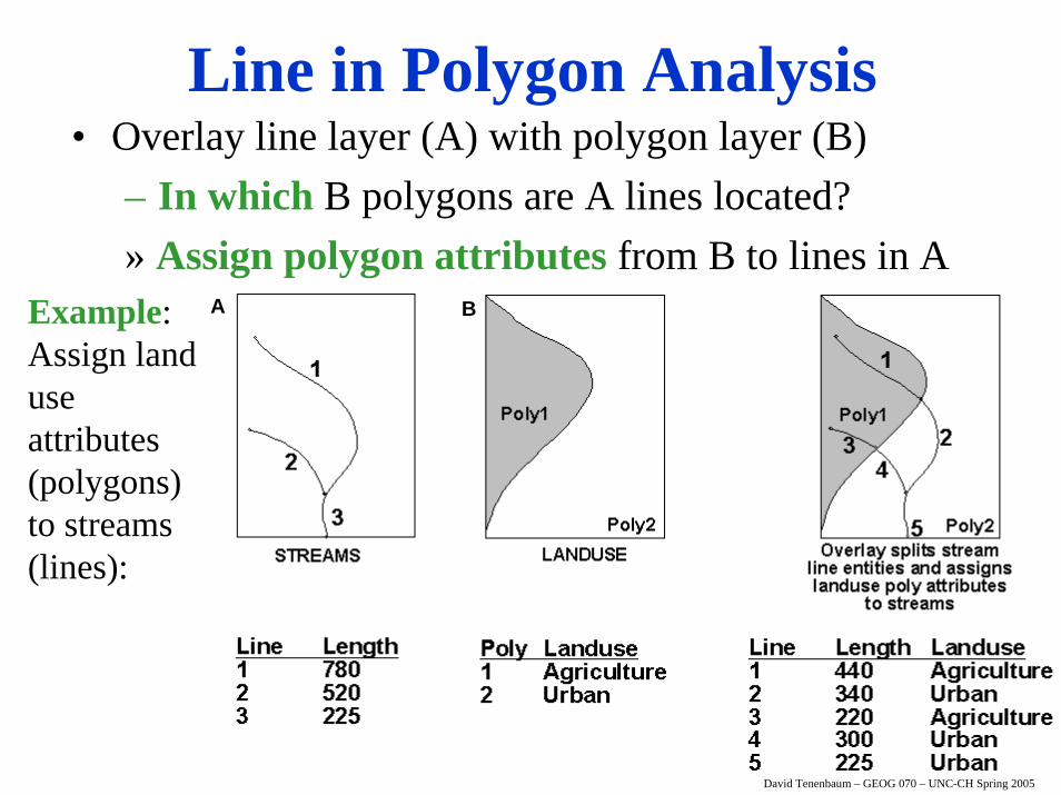
• Overlay line layer (A) with polygon layer (B)– In which B polygons are A lines located?» Assign polygon attributes from B to lines in A

A BExample: Assign land use attributes (polygons) to streams (lines):

Line in Polygon Analysis



Polygon Overlay Analysis• We can consider two different cases of analyses where

we compare two layers of polygons: • We can consider the case of discrete objects, where

individual polygon features make up a layer AND• We can also consider the field case, where a layer of

polygons consists of edge-to-edge polygons that fill the entire area of interest

• In the discrete object case: Find the polygons formed by the intersection of two polygons. There are instances where we might want to use this sort of analysis:• Do two polygons intersect?• Where area is in Polygon A but not in Polygon B?


Polygon Overlay, Discrete Object Case

•In this example, the unionof two polygons is taken to form nine new polygons. One is formed from both input polygons (1); four are formed by Polygon A and not Polygon B (2-5); and four are formed by Polygon B and not Polygon A (6-9)

A B

1

2

3

4

5

6 7

8

9


Polygon Overlay, Field Case• Two layers of edge-to-edge polygons are the

inputs, representing two thematic descriptions of the same area, e.g. soil type and land ownership information

• The two layers are overlaid, and all intersections are computed, creating a new layer:• Each polygon in the new layer has both a soil

type and land ownership information• The two attributes are said to be concatenated

• The task is often performed using the rasterspatial data model, but can use vector map algebra

Owner X

Owner Y

Public

•A layer representing a field of land ownership(symbolized using colors) is overlaid on a layer of soil type (layers offset for emphasis). The result after overlay will be a single layer with 5 polygons, each with land ownership information and a soil type

Polygon Overlay, Field Case


• Overlay polygon layer (A) with polygon layer (B)– What are the spatial polygon combinations of A and B?» Generate a new data layer with combined polygons

• attributes from both layers are included in output

• How are polygons combined (i.e. what geometric rules are used for combination)?– UNION (Boolean OR)– INTERSECTION (Boolean AND)– IDENTITY

• Polygon overlay will generally result in a significant increasein the number of spatial entities in the output– can result in output that is too complex too interpret

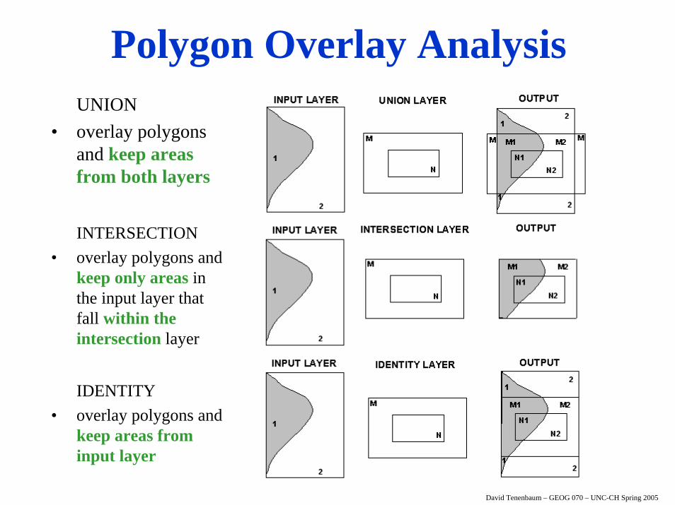
Polygon Overlay Analysis


UNION• overlay polygons

and keep areas from both layers

INTERSECTION• overlay polygons and

keep only areas in the input layer that fall within the intersection layer

IDENTITY• overlay polygons and

keep areas from input layer

Polygon Overlay Analysis


• Overlay analysis using the vector spatial data model is highly computationally intensive:– Complicated input layers can tax even current

processors• There is a tradeoff between the complexity vs.

the interpretability of results– Complex input layers with many polygons can

result in 100s or 1000s of resulting polygon combinations … can we make sense of all those combinations?

Problems with Vector Overlay Analysis (esp. Polygon)


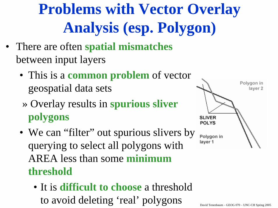
• There are often spatial mismatchesbetween input layers• This is a common problem of vector

geospatial data sets» Overlay results in spurious sliver

polygons• We can “filter” out spurious slivers by

querying to select all polygons with AREA less than some minimum threshold• It is difficult to choose a threshold

to avoid deleting ‘real’ polygons

Problems with Vector Overlay Analysis (esp. Polygon)

A B

The two input data sets are maps of (A) travel time from the urban area shown in black, and (B) county (red indicates County X, white indicates County Y). The output map identifies travel time to areas in County Y only, and might be used to compute average travel time to points in that county in a subsequent step

Overlay of Fields Represented as Rasters


A

•In both Venn probability diagrams and vector overlay analysis, we used UNION & INTERSECTION operations, corresponding to Boolean operations of OR & AND

UNION

INTERSECTION

A BOR B

A BAND A B

Boolean Operations

•We can apply these concepts in the raster spatial data model as well, but on a per cell basis with two input layers that contain true/false or 1/0 data:


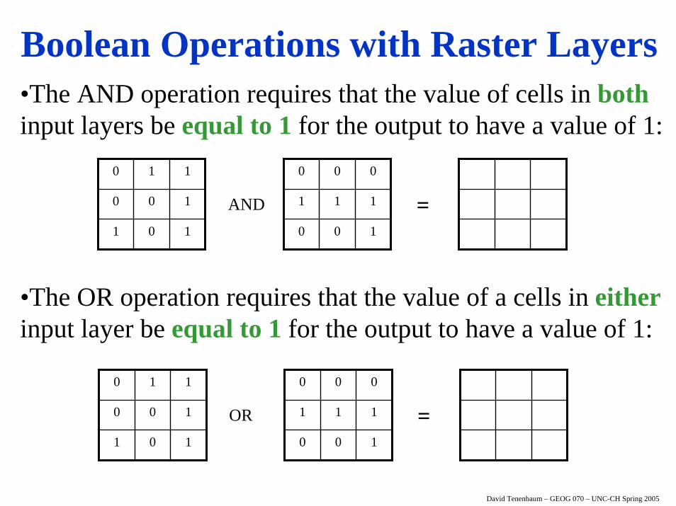
101

100

110

100

111

000

AND =

Boolean Operations with Raster Layers

101

100

110

100

111

000

OR =

•The AND operation requires that the value of cells in bothinput layers be equal to 1 for the output to have a value of 1:

•The OR operation requires that the value of a cells in eitherinput layer be equal to 1 for the output to have a value of 1:


Algebraic Operations w/ Raster Layers•We can extend this concept from Boolean logic to algebra•Map algebra:

•Treats input layers as numeric inputs to mathematical operations (each layer is a separate numeric input)•The result of the operation on the inputs is calculated on a cell-by-cell basis

•This allows for complex overlay analyses that can use as many input layers and operations as necessary•A common application of this approach is suitability analysis where multiple input layers determine suitable sites for a desired purpose by scoring cells in the input layers according to their effect on suitability and combining them, often weighting layers based on their importance


101

100

110

100

111

000

+ =201

211

110

Summation

101

100

110

100

111

000

× =100

100

000

Multiplication

101

100

110

100

111

000

+ =301

322

110

100

111

000

+

Summation of more than two layers

Simple Arithmetic Operations


Raster (Image) Difference

•An application of taking the differences between layers is change detection:

•Suppose we have two raster layers that each show a map of the same phenomenon at a particular location, and each was generated at a different point in time•By taking the difference between the layers, we can detect changes in that phenomenon over that interval of time

•Question: How can the locations where changes have occurred be identified using the difference layer?

517

656

345

723

541

653

- =-2-14

115

-3-12

The difference between two layers


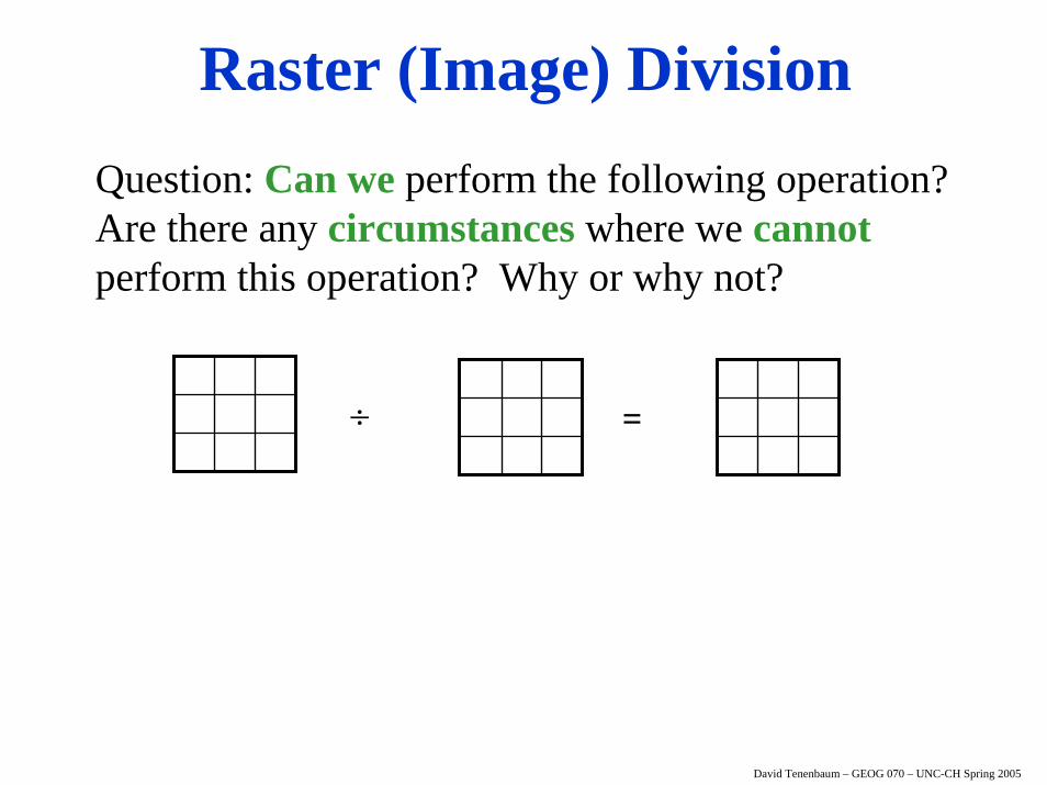
Question: Can we perform the following operation? Are there any circumstances where we cannotperform this operation? Why or why not?

÷ =

Raster (Image) Division


Linear Transformation

235

123

421

102

115

001

+ =100

111

000

+a b c

More Complex Operations

•We can multiply layers by constants (such as a, b, and c in the example above) before summation•This could applied in the context of computing the results of a regression model (e.g. output y = a*x1 + b*x2 + c*x3) using raster layers•Another application is suitability analysis, where individual input layers might be various criteria, and the constants a, b, and c determine the weights associated with those criteria


Spatial Interpolation• Often, we have a geographic phenomenon that we wish to

represent using a field (e.g. elevation), but the values of that field have been measured at sample points

• There is a need to estimate the complete field from the discrete samples, in order to• estimate values at points where the field was not

measured• create a contour map by drawing isolines between the

data points, or a raster digital elevation model which has a value for every cell

• Methods of spatial interpolation are designed to solve this problem


Inverse Distance Weighting (IDW)• A method of interpolation is inverse distance weighting:• The unknown value of a field at a point is estimated by

taking an average over the known values• Each known value is weighted by its distance from

the point, giving the greatest weight to the nearest points (thus the name inverse distance weighting, because as the distance between the point for estimation and the known point becomes greater, the weight is smaller)

• This is an implementation of Tobler’s Law since it is implicit in the inverse weighting scheme that points that are close together will tend to have similar values

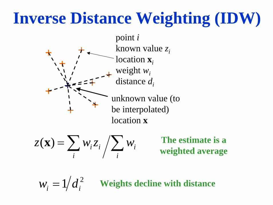
point iknown value zilocation xiweight widistance di

unknown value (to be interpolated)location x

∑∑=i

ii

ii wzwz )(x

21 ii dw =

The estimate is a weighted average

Weights decline with distance

Inverse Distance Weighting (IDW)


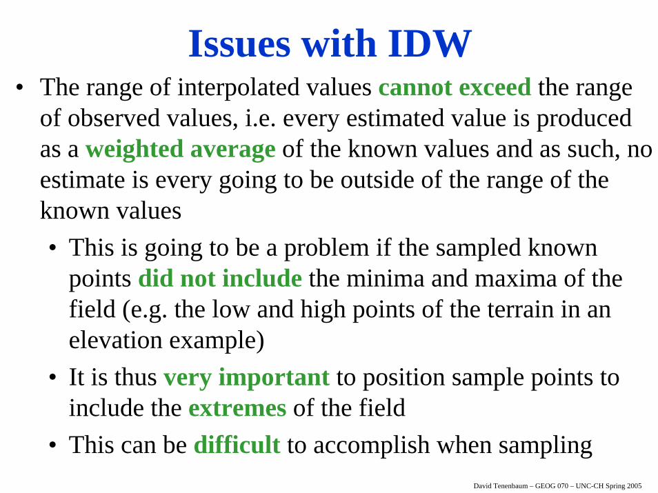
Issues with IDW• The range of interpolated values cannot exceed the range

of observed values, i.e. every estimated value is produced as a weighted average of the known values and as such, no estimate is every going to be outside of the range of the known values • This is going to be a problem if the sampled known

points did not include the minima and maxima of the field (e.g. the low and high points of the terrain in an elevation example)

• It is thus very important to position sample points to include the extremes of the field

• This can be difficult to accomplish when sampling


Issues with IDW•This set of six data points clearly suggests a hill profile (dashed line). But in areas where there is little or no data the interpolator will move towards the overall mean (solid line)•There are other interpolation methodsthat can do better in this situation …


Kriging• Kriging is a technique of spatial interpolation that is

firmly grounded in geostatistical theory• It extends the concept of distance-decay (as we saw used

in inverse distance weighting interpolation) by analyzing how the value of a variable changes with respect to distance using a scatter plot called a semivariogram

• Again we begin with sampled values from a field at known points

• Each possible pair of points is compared, producing:• A distance between the two points• A measure that describes the difference in values at

the two points, called semivariance• These values are then plotted in the semivariogram

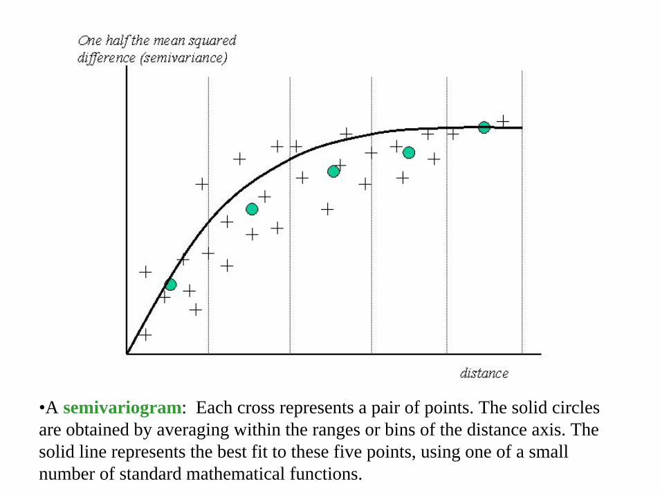
•A semivariogram: Each cross represents a pair of points. The solid circles are obtained by averaging within the ranges or bins of the distance axis. The solid line represents the best fit to these five points, using one of a small number of standard mathematical functions.


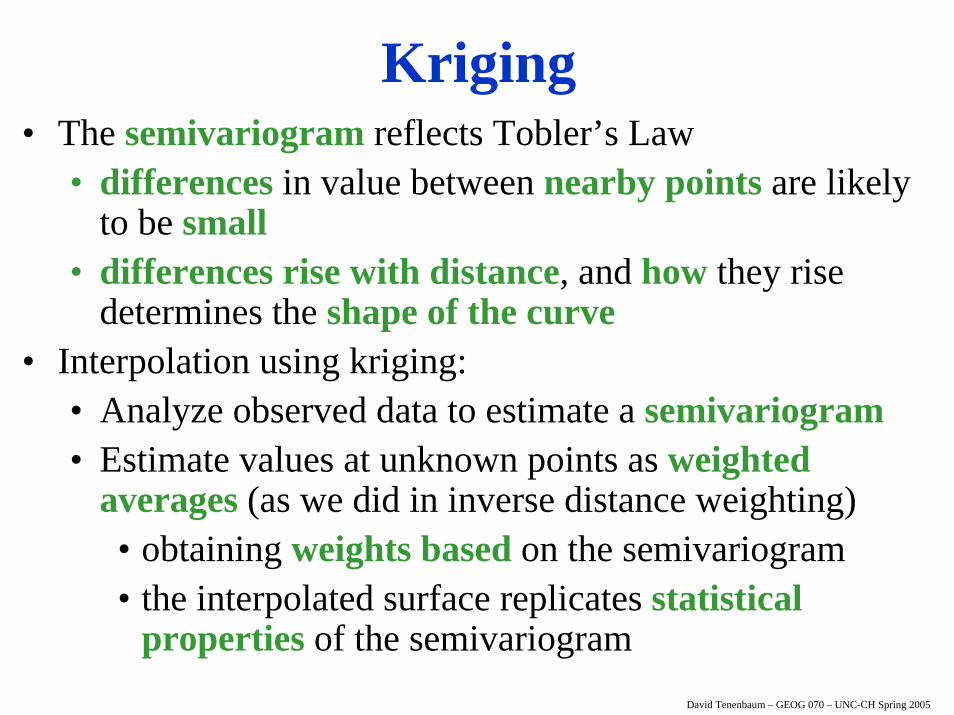
Kriging• The semivariogram reflects Tobler’s Law

• differences in value between nearby points are likely to be small

• differences rise with distance, and how they rise determines the shape of the curve

• Interpolation using kriging:• Analyze observed data to estimate a semivariogram• Estimate values at unknown points as weighted

averages (as we did in inverse distance weighting)• obtaining weights based on the semivariogram• the interpolated surface replicates statistical

properties of the semivariogram

definition of spatial analysis tenenbaum – geog 070 – unc-ch spring 2005 definition of spatial...

Documents