defense spending and fiscal multipliers: it’s all in the
TRANSCRIPT

Munich Personal RePEc Archive
Defense spending and fiscal multipliers:
it’s all in the variance
Rodriguez-Lopez, Jesus and Solis-Garcia, Mario
Universidad Pablo de Olavide, Macalester College
20 May 2018
Online at https://mpra.ub.uni-muenchen.de/86911/
MPRA Paper No. 86911, posted 23 May 2018 19:22 UTC
Defense spending and fiscal multipliers:
it’s all in the variance
Jesus Rodrıguez-Lopez
Universidad Pablo de Olavide de Sevilla
Carretera de Utrera 1
41003 Sevilla (Spain)
Mario Solis-Garcia∗
Macalester College
1600 Grand Avenue
St. Paul, MN 55105 (USA)
May 20, 2018
Abstract
We provide estimates of U.S. government expenditure multipliers for defense and non-defensespending over 1939-2014, using a fairly standard DSGE model that includes anticipated mili-tary spending changes (“war news shocks”), and find the following. First, our model’s war newsshocks compare favorably to Ramey’s (2011) narrative-based “defense news” shocks. Second,war news shocks have little effect on model variables regardless of the period under examina-tion. Unanticipated military expenditure accounts for substantial movements in output, butonly when observations from 1939 to 1954 are considered. Apart from that, movements in out-put are entirely driven by total factor productivity shocks. Third, our structural model cangenerate defense expenditure multipliers above unity under two conditions: (i) the multiplier iscalculated using the peak of the impulse-response function and (ii) a large number of observa-tions before and up to the Korean War are included. When multipliers are calculated accordingto Mountford and Uhlig’s (2009) present-value definition, they never exceed unity, regardless ofthe sample under analysis.
JEL codes: E32, E62, H56.Keywords: business cycles, news shocks, military expenditure, government multipliers.
∗Corresponding author. E-mail: [email protected]. We thank seminar participants at Macalester Col-lege, the 2017 Southern Economic Association meeting, and the 2017 Simposio de Analisis Economico. J. Rodrıguezacknowledges the financial support from the MINECO (Spain) project ECO2016-76818, and from Junta de Andalucıaunder project SEJ-1512.
1
1 Introduction
What portion of output fluctuations can be accounted by discretionary fiscal policy? Do differentkinds of public expenditure have the same impact on output? To what extent can governmentspending be anticipated? And is this anticipation more important for business cycles than fiscalsurprises? In this paper, we address these questions using a dynamic stochastic general equilibrium(DSGE) model for the U.S. economy. We differentiate between non-defense and defense spending,as wars can be taken as a natural experiment that allows to track the effects of transitory publicexpenditures over the economy.
A number of recent papers use military expenditure to explore the effects of fiscal policy onoutput: among others, Hall (2009), Barro and Redlick (2011), and Ramey (2009, 2011). These worksillustrate that defense outlays account for the bulk of the transitory component of U.S. governmentspending. Additionally, this variable can be taken as exogenous. By exploiting this exogeneity,these authors estimate fiscal multipliers both through simple regressions and structural vectorautoregression (SVAR) techniques. Following a narrative approach, Ramey (2009) compiles“defensenews” from Business Week and other newspapers across the 20th century that reflect beliefs aboutbuild-ups in military spending, and constructs an estimate of the change in the expected presentvalue of government spending. Ramey (2011) shows that SVARs generate biased estimates of thefiscal shock unless these defense news are added.
Different from Ramey (2011), we adopt a non-narrative approach to uncover anticipated militaryexpenditure shocks, following the methodology proposed by Beaudry and Portier (2004, 2007) andextended by Schmitt-Grohe and Uribe (2012), who focus on news of forthcoming technologicalprogress. We work upon these studies and consider “war news shocks,” understood as anticipationsof defense spending changes. To our knowledge, we are the first to incorporate this variable withinthe news shock literature. While we share Ramey’s strategy of using defense spending to identifythe shocks, our identification is based on a fairly standard DSGE model with real frictions, nonominal rigidities, and where the war news shocks and structural parameters are estimated withBayesian techniques. Therefore, our impulse response functions and fiscal multipliers are basedupon a structural model and not an SVAR.
Our model also considers a set of fiscal rules for government expenditure and taxes followingLeeper, Plante, and Traum (2010). Both public expenditure and tax rates respond to business cycleconditions (i.e., automatic stabilizers) and to the state of debt. Unlike the contribution of Leeperet al., we extend the fiscal component of our model in two directions. First, public expenditure isdecomposed into defense and non-defense spending, where the former is fully exogenous from outputand debt, and the latter is adjusted when the defense budget is activated.1 Second, the fiscal rulesare augmented by the war news shock, so that military expenditure changes can be anticipated asconflicts and war episodes loom in the horizon, and the effect of anticipation remains orthogonalto other fiscal shocks and allows us to accurately measure the defense spending multiplier.
We use a yearly sample that runs from 1939 to 2014—a period that contains several warepisodes—and this allows us to gauge the effects that defense (and other kinds of) spending has overU.S. aggregate fluctuations. We start by estimating a fiscal multiplier based on defense spending—along the line suggested by Hall (2009), Barro and Redlick (2011), and Ramey (2011)—that relieson the correlation between output growth and defense spending growth. Our results suggest that abreak in the estimate of the multiplier occurs around the onset of the Korean War. This result hasbeen highlighted by Ramey (2011). Guided by this evidence, we decide to split the sample into two
1 Hence, non-defense expenditure is more elastic than its defense counterpart, an assumption consistent with theconduction of fiscal policy during war times. In the model, if military expenditure needs to increase, the governmentbudget automatically reduces non-defense spending.
2
periods: one that spans 1939 to 1954, covering World War II (hereafter, WWII) and the KoreanWar, and another from 1955 to 2014, a period with war episodes whose volume of spending areof minor importance than those in the first one. Section 3 offers additional insights regarding ourdecision to split the sample in two.
Our results can be summarized in three main points. First, we show that our DSGE-basedmodel does a good job in uncovering the war news shocks, relative to the defense news identified bythe narrative approach of Ramey (2011). The correlation coefficient between both series is positiveand moderately high. Comparing them over time, our war news shocks correctly anticipate thegovernment spending increase of WWII, although the Korean War appears as a surprise. For theremaining conflicts, the shocks from both approaches overlap. We conclude that our DSGE modelis a valid framework to identify anticipated changes in defense spending—at least for the U.S.
Second, a variance decomposition exercise suggests that unanticipated military expenditureshocks generate substantial movements in output in the sample that includes WWII and the KoreanWar. For the second sample, fiscal spending shocks play a minor role on model variables; instead, thebulk of the variability of the model variables is mostly accounted by total factor productivity (TFP)shocks. Surprisingly, we find that the war news shock is of secondary importance in both samples.In addition, the simulated moments generally reproduce observed moments in the business cyclecorrelogram for both periods. Interestingly, model simulations imply a decline in the correlationbetween output and defense spending for the second sample relative to the first one, which implya fall in the OLS estimates of the multiplier, a fact also noted by Hall (2009), Barro and Redlick(2011), and Ramey (2011), after the Korean War.
Finally, we calculate a set of multipliers, based on defense and non-defense government expendi-ture, following two alternative definitions. The first definition follows the present-value multipliersproposed by Mountford and Uhlig (2009). We find that these values never exceed unity, regard-less of the expenditure series considered; in the short run, the range is [0.75, 0.81] for non-defenseexpenditure and [0.59, 0.67] for military spending. The second definition of multiplier is based onthe peak of the model’s impulse-response function. In this case, we do find multipliers above unityfor defense spending: 2.19 when the full sample is considered and 6.11 for the sample that runsfrom 1939 to 1954, which includes two major war episodes. We argue that this result is due to amoderation in the variance of the structural fiscal shocks observed after the Korean War, whichmainly affected defense spending. Regardless of the sample or the definition, multipliers based ondefense expenditure are never larger than 0.8.2
The paper is structured as follows. Section 2 briefly surveys related research. Section 3 intro-duces some preliminary evidence concerning U.S. government spending and estimates of the fiscalmultiplier. The DSGE model and the fiscal rules are presented and described in Section 4. Section5 reports our main results: the identified news of war, impulse-responses, variance decompositions,and fiscal multipliers. The last section offers several concluding remarks.
2 Related literature
This paper is connected with three branches of research. The first is related to studies that havehighlighted the role of anticipation on business cycles. The second brand of research deals withassessing how fiscal policy affects economic activity and the estimation of fiscal multipliers. The last
2 As a publicly-provided public good—like street lighting or a well-functioning legal system—defense spending hasa reduced margin for discretional changes, which reduces its usefulness as a fiscal policy tool. While our model isable to generate multipliers above unity when considering defense spending in a sample that includes WWII and theKorean War, this shouldn’t be considered as an endorsement to use war to stimulate the economy.
3
one is focused on anticipation of warfare and conflicts through information content in newspapersor in financial assets and aggregate series, such as defense spending.
News shocks The path-breaking papers by Beaudry and Portier (2004, 2007) set forth a researchprogram that explores how news of forthcoming neutral technological progress affect current deci-sions. This research was later extended by Schmitt-Grohe and Uribe (2012) to incorporate otherkinds of news shocks (e.g., government expenditure, investment-specific technological progress,wage-markup, or preference shocks); they find that news shocks can account for about 50% of thevariance of output, consumption, investment, and hours worked. Born, Peter, and Pfeifer (2013)offer a refinement of Schmitt-Grohe and Uribe by incorporating anticipated changes in capital andlabor tax rates in a New Keynesian DSGE model. While they share Schmitt-Grohe and Uribe’sconclusion that anticipated variables are important determinants of the business cycle, they findthat fiscal shocks (both anticipated and unanticipated) have little impact over real variables.
Another line of research has extended this methodology to focus solely on anticipated changes intaxes and spending. Mertens and Ravn (2011) analyze whether a DSGE model can account for theeffect of anticipated and unanticipated changes in federal tax liability changes; by including habitformation, variable capacity utilization, adjustment costs, and consumer durable spending, they findthat the model can account for most of the empirical responses to a fall in tax liabilities. Whilenot necessarily stressing the role of news shocks, the New Keynesian model in Leeper, Traum, andWalker (2017) allows for anticipation in government expenditure and transfers. After performinga prior predictive analysis3 between different modeling frameworks, they select a New Keynesianspecification that includes government expenditure in the utility. Taking their model to the data,they find evidence supportive of multipliers above unity in the short run, in the range [0.93, 1.41].Ben Zeev and Pappa (2017) calculate a series for defense news shocks following the SVAR-basedidentification approach of Barsky and Sims (2011), and find that expected changes in defensespending have sizable effects on output, hours worked, inflation, and the interest rate. By contrast,as we comment later, we find that military spending (anticipated or not) plays a reduced role inU.S. fluctuations, especially during the last decades.
Expenditure and business cycles The fiscal multiplier can be defined as the output changerelative to a discretionary fiscal variation; i.e., a change in non-automatic fiscal incentives. Theoriginal definition of the multiplier dates back to Keynes’s ideas—later developed by the Keynesianschool—through the concept of marginal propensity to consume (MPC). As is usually explained inintroductory textbooks, since MPC ∈ (0, 1), the multiplier is given by 1/(1−MPC) > 1. However,the literature has not reached a consensus regarding the empirical value of the fiscal multiplier. Forexample, Spilimbergo, Symansky, and Schindler (2009) calculate multipliers for different countriesand find that the values are within the interval [−1.5, 5.2]. Hall (2009) concludes that the multipliermay range from 0.7 to unity for the U.S. economy; he argues that a multiplier value of 1.7 couldbe reached if the nominal interest rate has hit the zero lower bound.
Many authors have estimated the multiplier using SVARs. We count, among many others:Blanchard and Perotti (2002), Galı, Lopez-Salido, and Valles (2007), Perotti (2008), Mountfordand Uhlig (2009), Ramey (2011), Auerbach and Gorodnichenko (2012), and Ramey and Zubairy(2018). Aside from the last three papers in this list, these multiplier estimates are based onorthogonalization conditions that generate a set of structural shocks from forecasting errors. Manyof these SVAR-based studies propose using defense spending as a tool to identify the fiscal shocks,
3 See Geweke (2010, chap. 3).
4
given that it is considered exogenous to output. Under this identification scheme, the impulse-response functions from fiscal shocks are used to estimate the value of the multiplier. These authorsprovide output multipliers that range between 0.3 and 0.9 on impact, and reaching values aboveone for peak impulse-responses after several quarters.
As we have already mentioned, Ramey (2011) warns that a portion of fiscal shocks identifiedusing SVAR tools might be anticipated, so that they cannot be used to assess the fiscal multiplier.Instead, she uses the defense news collected from her narrative approach; as long as the series reflectsbeliefs about future changes in military spending, they allow her to identify unanticipated fiscalshocks. She estimates peak impulse multipliers between 1.1 and 1.2.4 Auerbach and Gorodnichenko(2012) use both the identification strategy of Blanchard and Perotti (2002) and the defense newsseries of Ramey (2011) to calculate multipliers during expansions and recessions; they find thatusing Ramey’s values generates larger values in both cases. Ramey and Zubairy (2018) elaborateon the work of Ramey (2011) by first building a quarterly-frequency GDP series that runs from1889 to 2015. Using this expanded dataset, they ask whether the size of the multiplier depends onslack conditions (e.g., high vs. low unemployment) or the presence zero lower bound. In general,they cannot find evidence for large multipliers in the former scenario, but do find multipliers aboveunity when certain conditions are met in the latter one.
Regarding DSGE models, Cogan, Cwik, Taylor, and Wieland (2010) show that standard NewKeynesian models (e.g., Smets and Wouters 2007) cannot generate multipliers above unity under apermanent increase in government expenditure; they ask whether adding non-Ricardian consumers(Galı et al. 2007) can offer higher values, but find it cannot. Zubairy (2014) uses a model withnominal frictions, deep habits,5 and a rich fiscal policy block with automatic stabilizers to findmultipliers that are above unity in the short run. We should add that neither of these modelsconsiders anticipation effects.
Anticipation of warfare Finally, forecasting conflicts has received increasing attention withinthe fields of economics and political science using, for instance, newspaper texts as in Ramey(2011, see also Chadefaux 2014, Mueller and Rauh 2017, and the references therein). Overall,this literature finds that war episodes are hardly predictable. Other research studies how financialvariables incorporate information about the likelihood of a conflict: Hall (2004) does so for the Swissexchange rate during World War I and Rigobon and Sack (2005) for the Iraq War in 2003. Similarly,Chadefaux (2017) reports evidence that market participants tend to underestimate the risk of war,and react with surprise immediately thereafter. Using long run series of government bond yieldsfrom 1816 through 2007, for France, the UK, and Germany, he finds that market participants havehistorically underestimated the probability of war prior to its outbreak, and the onset typically ledto a large correction. Although our intention is not to predict the onset of warfare, we use thesmoothed shocks from the estimation procedure to identify the news of war implied by our model.
3 Preliminary evidence
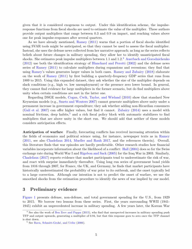
Figure 1 presents defense, non-defense, and total government spending for the U.S., from 1929to 2015. We borrow two lessons from these series. First, the years surrounding WWII (1941-1945) exhibit an unprecedented increase in military spending. A few years later, the Korean War
4 See also the work of Ben Zeev and Pappa (2015), who find that unexpected increases in military spending pushTFP and output upwards, generating a multiplier of 0.94, but that this response goes to zero once the TFP channelis shut down.
5 See Ravn, Schmitt-Grohe, and Uribe (2006).
5
1930 1940 1950 1960 1970 1980 1990 2000 2010 20150
0.05
0.1
0.15
0.2
0.25
0.3
0.35
0.4
0.45
0.5
Year
Perc
ent of G
DP
↓ World War II (1944), 43.3%
Korean War (1953), 15.7%
Vietnam War (1967), 11.0%
Reagan buildup (1982−5), 7.3%Gulf War (1991), 6.7%
War in Afghanistan (2002), 4.2% ↑
Total government spending
Defense
Non−defense
Figure 1: Government expenditure (total, defense, and non-defense), 1929-2015.
brought an increase in defense spending, but of smaller magnitude relative to WWII (the defensespending series peaks a bit over 43% of GDP in 1944; its value in 1953 is considerably lower at16% of GDP). Nonetheless, defense expenditure accounts for the bulk of the transitory componentin total government expenditure. Second, there is a budgetary tradeoff in defense and non-defenseexpenditure—particularly evident in the decades after the Korean War.
A straightforward way to quantify the relation between output and government spending is theregression
∆YtYt−1
= a+mY
∆Mt
Yt−1
+ et, (3.1)
where Yt and Mt denote real GDP and defense expenditure at time t. This specification is used byHall (2009) and Barro and Redlick (2011), who show that the OLS estimator mY can be interpretedas a weighted-value output multiplier
mY =cov(∆Yt/Yt−1,∆Mt/Yt−1)
var(∆Mt/Yt−1)=
∑
t
(
∆Mt
Yt−1
)(
∆Yt
Yt−1
)
∑
t
(
∆Mt
Yt−1
)2=
∑
t
ωt
∆Yt∆Mt
,
with weight ωt ≡(
∆Mt
Yt−1
)2/∑
t
(
∆Mt
Yt−1
)2.
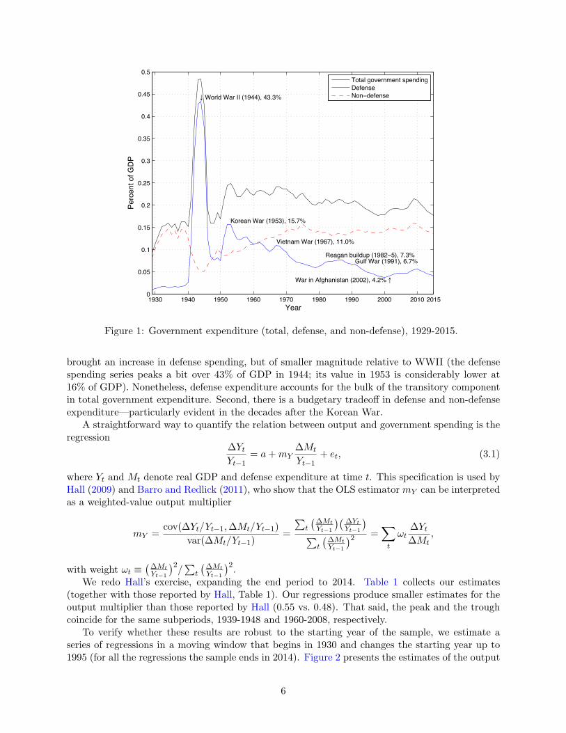
We redo Hall’s exercise, expanding the end period to 2014. Table 1 collects our estimates(together with those reported by Hall, Table 1). Our regressions produce smaller estimates for theoutput multiplier than those reported by Hall (0.55 vs. 0.48). That said, the peak and the troughcoincide for the same subperiods, 1939-1948 and 1960-2008, respectively.
To verify whether these results are robust to the starting year of the sample, we estimate aseries of regressions in a moving window that begins in 1930 and changes the starting year up to1995 (for all the regressions the sample ends in 2014). Figure 2 presents the estimates of the output
6
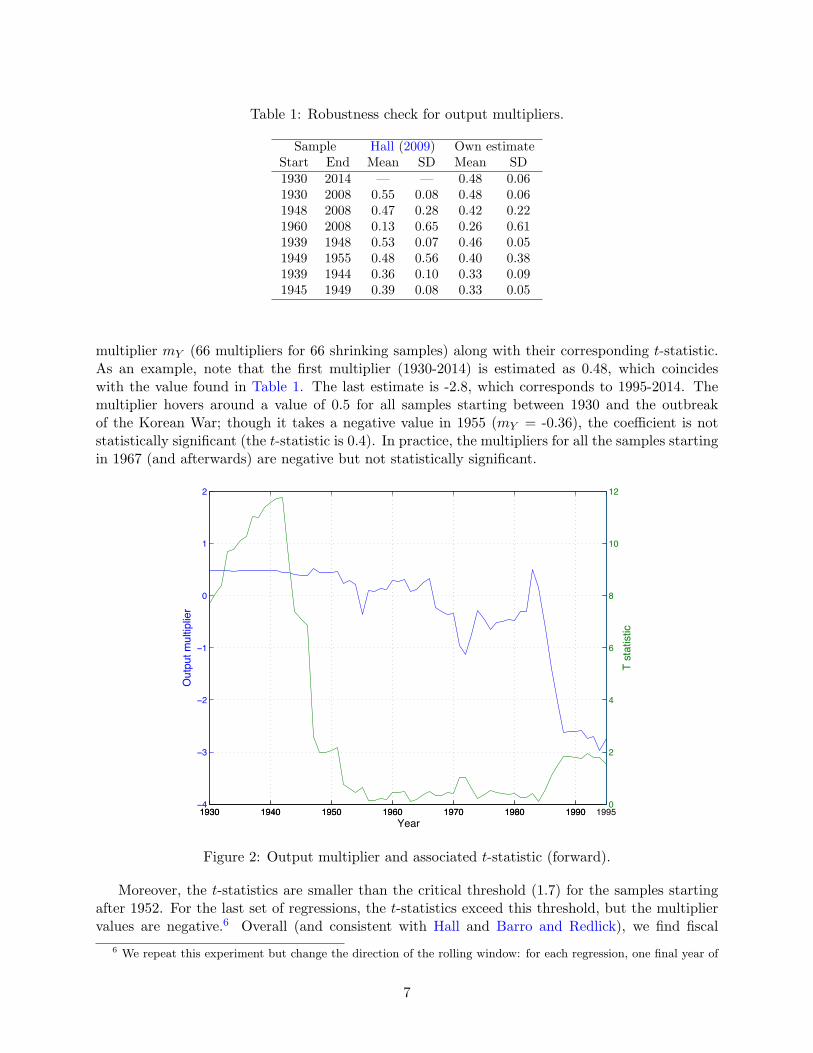
Table 1: Robustness check for output multipliers.
Sample Hall (2009) Own estimateStart End Mean SD Mean SD1930 2014 — — 0.48 0.061930 2008 0.55 0.08 0.48 0.061948 2008 0.47 0.28 0.42 0.221960 2008 0.13 0.65 0.26 0.611939 1948 0.53 0.07 0.46 0.051949 1955 0.48 0.56 0.40 0.381939 1944 0.36 0.10 0.33 0.091945 1949 0.39 0.08 0.33 0.05
multiplier mY (66 multipliers for 66 shrinking samples) along with their corresponding t-statistic.As an example, note that the first multiplier (1930-2014) is estimated as 0.48, which coincideswith the value found in Table 1. The last estimate is -2.8, which corresponds to 1995-2014. Themultiplier hovers around a value of 0.5 for all samples starting between 1930 and the outbreakof the Korean War; though it takes a negative value in 1955 (mY = -0.36), the coefficient is notstatistically significant (the t-statistic is 0.4). In practice, the multipliers for all the samples startingin 1967 (and afterwards) are negative but not statistically significant.
1930 1940 1950 1960 1970 1980 1990 1995−4
−3
−2
−1
0
1
2
Year
Ou
tpu
t m
ultip
lier
1930 1940 1950 1960 1970 1980 19900
2
4
6
8
10
12
T s
tatistic
Figure 2: Output multiplier and associated t-statistic (forward).
Moreover, the t-statistics are smaller than the critical threshold (1.7) for the samples startingafter 1952. For the last set of regressions, the t-statistics exceed this threshold, but the multipliervalues are negative.6 Overall (and consistent with Hall and Barro and Redlick), we find fiscal
6 We repeat this experiment but change the direction of the rolling window: for each regression, one final year of
7

multipliers around 0.5, but only when our sample includes WWII and the Korean War. In oursecond sample, the fiscal multiplier estimates are not statistically significant—so they must betaken as zero. Samples that include recent military episodes, such as the Gulf War or the conflictin Afghanistan, cannot generate fiscal multipliers of the same magnitude reported by Barro andRedlick (2011) or Hall (2009).
Following Ohanian (1997), Ramey (2011) argues that for samples starting after 1954, the declin-ing fiscal multiplier can be attributed to the different fiscal instruments used by the U.S. governmentin both wars. Indeed, Ohanian claims that the distortions resulting from the tax increase in theKorean War were higher than those produced from higher debt in WWII. Guided by this evidenceand Ramey (2011)’s arguments, we split the sample in two: a first sample that considers 1939 to1954—which includes both WWII and the Korean War—and another from 1955 to 2014, a periodwith war episodes whose volume of spending are of minor importance than those of the first one.
4 The benchmark model
The model economy has three kinds of agents: a representative household, a representative firm,and a government. We discuss each of these in turn and then present a notion of equilibrium.
4.1 Household
We assume that the economy is inhabited by a representative household whose utility function de-pends on consumption and hours worked. Household’s decisions are constrained by a budget: grossincome must be distributed between consumption, savings, and taxes. Saving can be done througha government bond or a physical capital. Our model also includes habit formation in consumptionand capital adjustment costs. In particular, the household chooses sequences of consumption ct,labor supply nt, investment xt, utilization rate of capital ut, and bond holdings bt to solve thefollowing problem:
max E0
∞∑
t=0
βt log(ct − µct−1)− φn1+χt
1 + χ(4.1)
s.t. ct + xt + bt = rtutkt + wtnt + rbtbt−1 − ζt (4.2)
ζt = τktrtutkt + τntwtnt + τctct − τt − δ(ut)τktkt (4.3)
kt+1 = (1− δ(ut))kt + xt[1− S(xt/xt−1)]. (4.4)
In the above, β ∈ (0, 1) is a discount factor, µ ∈ [0, 1) is a parameter governing habit persistence,φ > 0 controls the relative weight of consumption and leisure, and χ > 0 denotes the inverse ofthe Frisch elasticity of labor supply. Equation (4.2) represents the household’s budget constraint:the stock of physical capital is denoted by kt, which is rented to the representative firm at a rentalrate rt. The real wage is denoted by wt. In addition, rbt denotes the gross rate of return ongovernment bonds (the rate is fixed in period t− 1) and ζt denotes the fiscal policy component ofthe household budget. Following (4.3), the nonnegative processes {τkt, τnt, τct} represent tax rateslevied over capital income, labor income, and the purchase of consumption goods, respectively, whileτt denotes government lump-sum transfers/taxes. The last term in (4.3) represents a depreciationallowance. Equation (4.4) is the law of motion for capital, where the depreciation rate δ depends
the sample is added, taking the starting period 1930 to 1950 as fixed. In this case, the multiplier hovers around 0.48while the statistical significance of these estimates displays an upward trend (as one year is added at the end of thesample) that is always above the critical threshold.
8
on capital utilization and there are investment adjustment costs parametrized by function S. Weimpose the following functional forms over δ and S:
δ(ut) = δ0 + δ1(ut − 1) +δ22(ut − 1)2 (4.5)
S(xt/xt−1) =κ
2(xt/xt−1 − 1)2. (4.6)
Equation (4.5) shows that the depreciation of physical capital is a (quadratic) function of theutilization rate ut. We normalize the stationary capital utilization rate to u = 1; thus, δ0 ∈ (0, 1)is the steady state depreciation rate of the capital stock and δ1, δ2 ≥ 0 are parameters of thedepreciation function. Finally, equation (4.6) characterizes the (quadratic) adjustment cost ofinstalling new capital.
As usual, we assume that the household behaves competitively and takes the processes for prices{rt, wt, r
bt}
∞
t=0 and fiscal policy {τkt, τnt, τct, τt}∞
t=0 as given when it makes its decisions.
4.2 Firm
The representative firm rents capital KFt and labor services NFt from the household and transformsthem into output yt. We assume that the firm behaves competitively, takes the processes for therental prices {rt, wt}
∞
t=0 as given, and solves the following profit maximization problem:
max AztKαFtN
1−αFt − rtKFt − wtNFt
s.t. KFt, NFt ≥ 0.
In the above, A > 0 is a scaling factor, α ∈ (0, 1) represents the capital share, and zt is a stationarytechnology disturbance. We assume that zt follows
log zt = (1− ρz) log z + ρz log zt−1 + εzt, (4.7)
where z is the steady-state level of zt, ρz ∈ (0, 1) is a persistence parameter, and εzt is an i.i.d. processwith mean zero and standard deviation σz.
4.3 Government and fiscal rules
The government trades bonds Bt with the household and levies taxes over consumption and capitaland labor income. It uses these resources to finance bond payments rbtBt−1 and exogenous sequencesof military purchases mt and non-military consumption gt. Lump-sum transfers τt are positiveif resources are rebated from the public sector to the households and negative otherwise. Thegovernment’s budget constraint is
gt +mt + rbtBt−1 + τt = Bt + τktrtutkt + τntwtnt + τctct − δ(ut)τktkt. (4.8)
We specify a set of fiscal rules for public spending, transfers, and tax rates. In these rules, variableswithout a time subindex denote a stationary position. We assume that defense spending mt doesnot respond to output or the state of public debt—our way of addressing the non-discretionarybehavior of the variable—and require it to follow the law of motion
(mt −m) = ρm (mt−1 −m) + εmt + εwarm,t−1. (4.9)
Equation (4.9) indicates that military spending mt evolves with relative persistency ρm and thatdeviations from its steady state can be due to a pure (non-anticipated) fiscal shock εmt or the war
9
news shock εwarm,t−1, which becomes known one period in advance. The war news shock is key toproperly measuring the effects of military expenditure over the economy, as changes in the variableare often anticipated. Both innovations are i.i.d. processes with mean zero and standard deviationσm and σwar, respectively.
Non-defense expenditure follows an augmented version of the fiscal rule suggested by Leeperet al. (2010):
(gt − g) = ρg (gt−1 − g)− θmg (mt −m)− θyg (yt−1 − y)− θbg (bt−1 − b) + εgt. (4.10)
From (4.10), gt adjusts automatically to past values and in response to defense spending (seeFigure 1), the business cycle, and the state of debt. Hence, there is a systematic correction innon-defense spending when (1) defense spending differs from its steady-state value m, (2) outputfluctuates around its steady state position, or (3) debt accumulates relative to the stationary state.Parameters
{
θmg , θyg , θbg}
are expected to be positive. Finally, non-defense spending is impulsed bya fiscal shock εgt, which is an i.i.d. process with mean zero and standard deviation σg.
The remaining fiscal rules are specified as in Leeper et al.:
(τt − τ) = ρτ (τt−1 − τ)− θyτ (yt−1 − y)− θbτ (bt−1 − b) + ετt, (4.11)
(τkt − τk) = ρk(τk,t−1 − τk) + θyk(yt−1 − y) + θbk(bt−1 − b) + εkt, (4.12)
(τnt − τn) = ρn(τn,t−1 − τn) + θyn(yt−1 − y) + θbn(bt−1 − b) + εnt, (4.13)
(τct − τc) = ρc(τc,t−1 − τc) + εct. (4.14)
Except for the consumption tax rate, there is an automatic response with respect to output fluc-tuations and to the level of debt:
{
θyτ , θbτ , θyk, θ
bk, θ
yn, θbn
}
are expected to be positive. Unlike Leeperet al., we assume that the non-anticipated fiscal shocks are all orthogonal. These fiscal impulsesare i.i.d. processes with mean zero and standard deviation σj for j = {τ, k, n, c}.
Finally, the feasibility constraint of the economy dictates that output must be either consumed(by households or by the government) or invested:
yt = ct + xt + gt +mt. (4.15)
4.4 Equilibrium
Let ξt = (kt, bt) denote the vector of individual state variables. Given a government policy,
{gt,mt, τt, τkt,, τnt, τct} ,
a competitive equilibrium is a set of decision rules {c(ξt), n(ξt), u(ξt), k(ξt−1), b(ξt−1)}, aggregatechoices {C(ξt), NF (ξt),KF (ξt−1), B(ξt−1)}, and prices {w(ξt), r(ξt), r
bt (ξt)}, such that
1. Given the government policy and factor prices, the household’s utility is maximized, subjectto the budget constraint and the state equation for capital.
2. Factors of production (labor and capital) are hired at their marginal productivities.
3. The government satisfies its budget equation given the fiscal rules.
4. Markets clear: labor demand is equal to labor supply, capital demand is equal to capitalsupply, and the aggregate feasibility condition holds.
10
5. The representative agent condition holds; i.e., aggregate choices coincide with individual oneswhen the latter is representative:
C(ξt) = c(ξt)
NF (ξt) = n(ξt)
KF (ξt−1) = u(ξt)k(ξt−1)
B(ξt−1) = b(ξt−1).
5 Results
5.1 Estimation
We first provide some details regarding the parametrization of the model. In an initial step, wecalibrate a subset of parameters and steady state values using sample averages, and then useBayesian techniques to estimate the remaining ones.
Table 2 introduces the set of parameters determined ex-ante, together with the target valuesthat the model aims to reproduce in the steady state. The capital income share is set to α = 1/3for both samples. We normalize steady state output to unity and GDP components are expressedin relative terms, using sample averages of U.S. accounts. Stationary tax rates are calculated asan average of calculated values (see Appendix A for details on data construction). Between thetwo samples, the main difference concerns the composition and magnitude of public expenditure,disaggregated into defense and non-defense spending. Consumption relative to output is stablearound 0.54, while investment moves opposite total government spending.
Table 2: Parameters determined ex-ante and target values.
Before Korean War After Korean War Full sample1939-1954 1955-2014 1939-2014
ParameterCapital income share α 0.333 0.333 0.333Capital income tax rate τk 0.346 0.262 0.279Labor income tax rate τn 0.108 0.189 0.172Consumption tax rate τc 0.052 0.052 0.052TargetNormalized output y 1.000 1.000 1.000Consumption c 0.541 0.543 0.542Investment rate x 0.198 0.250 0.239Non-defense spending g 0.088 0.135 0.125Defense spending m 0.172 0.072 0.093Lump-sum transfers τ -0.148 -0.044 -0.066Debt-to-output b/y 0.770 0.526 0.577Capital utilization u 1.000 1.000 1.000
After log-linearizing the model, we estimate the remaining parameters using Bayesian tech-niques. The following nine series are assumed to be observable: output yt, consumption ct, defenseand non-defense government spending {mt, gt}, transfers τt, tax rates {τkt, τnt, τct}, and debt bt.
11
Table 3 presents the prior and posterior distributions that result from the econometric exercise.The habit persistence parameter µ increases in value for the second sample, from 0.74 to 0.83. Theestimated Frisch elasticity of labor changes from 1.87 in the first sample to 0.67 for the second.7
The estimates for {δ0, δ2, κ} show standard values (see Leeper et al.), while the cost on capitaladjustment κ increases.
Combining the parameters of the first panel in Table 3 with the targets reported in Table 2,the model is calibrated for the U.S. economy for the different samples. Table 4 summarizes theseresults. The annual capital-output ratio is 2.28 on the full sample. The long-run bond treasuryrates are 4.4, 2.4, and 3.0%, which imply a subjective discount rate of β ∈ [0.957, 0.976]. The rentalprice r, the linear component δ1 from the depreciation function, the utility weight φ, and the scalingparameter A in the production function are calculated using the steady state conditions.
Table 5 reports the prior and posterior distributions; we believe that four results are worthnoting. First, the persistency of fiscal rules and the TFP shocks has increased following the end ofthe Korean War. Second, non-defense spending declines in response to military spending build-upas −θmg is negative in both samples. Third, in the post-Korean War sample, the tax rates exhibita higher response to variations in output, but a smaller response to variation in debt.
Finally, as the bottom panel in Table 5 shows, all standard deviations are smaller in the secondperiod. This moderation affects not only the volatility of the TFP shock σz, but also those ofthe the fiscal shocks σj for j = {m, g, τ, k, n, c}. Of major importance is the moderation in thevolatility of military spending σm and that of the war news shock σwar, lower by a factor of 27 and12, respectively. The standard deviations for the tax rates also experience a sensible moderation,becoming between 1.8 and 4.0 times smaller.8
5.2 Identifying the news of war
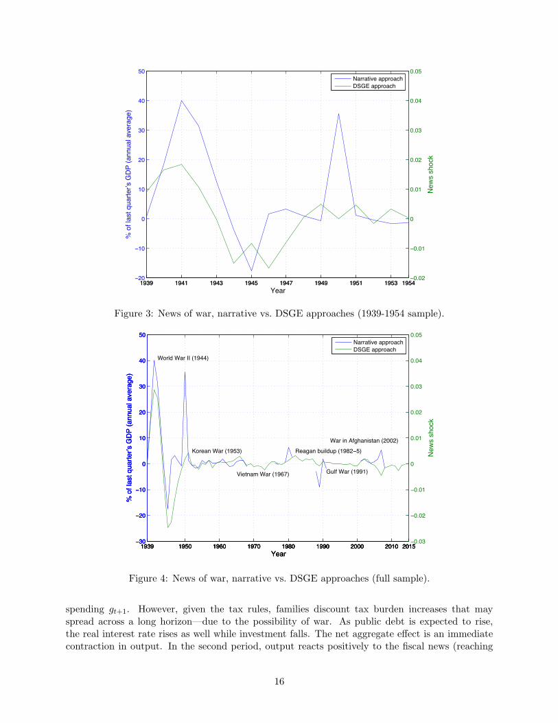
We use the smoothed shocks from the estimation procedure to identify the news of war implied byour model. To this end, Figures 3 and 4 compare the war news shocks obtained from our model tothe defense news derived from the narrative approach of Ramey (2011).
Figure 3 considers the first sample, 1939-1954. The DSGE-based approach does a good job incapturing the dynamics of the defense news of Ramey (2011). Note that for 1946, the narrativeapproach suggests an increase in the defense while our approach shows a fall in the value of thewar news shock; this seems to be consistent with the fact that the war ended by 1945, just a yearbefore. While the DSGE-based shocks reproduce the ones from the narrative approach for WWII,our results suggest that the Korean War was largely unanticipated.9
Figure 4 replicates the results from Figure 3 using the full sample estimation results. (Thisexplains why the values for 1939-1954 are not identical to those in Figure 3.) Even though thenarrative approach series has gaps in the values provided, our estimates track these results fairlywell.10 For the remaining war episodes, our non-narrative approach anticipates a larger fractionof fiscal increases in military spending relative to Ramey’s approach. For instance, our model
7 Heathcote, Storesletten, and Violante (2010) and Chetty, Guren, Manoli, and Weber (2011)—who use a marriedcouple as the notion of household—propose an estimate of 0.72.
8 Fernandez-Villaverde, Guerron-Quintana, Kuester, and Rubio-Ramırez estimate fiscal rules for spending and taxrates with time varying volatility. The do not consider anticipated changes in government spending or the tax rates,though. They report evidence that these shocks to the time varying volatility of fiscal variables can produce adverseeffects on economic activity.
9 Secretary of State Dean Acheson, during his speech in the National Press Club in January 1950, did not considerthe Korean Peninsula to be a part of the all-important “defense perimeter” of the U.S. The Korean War broke outshortly after, on June 25 1950.
10 The correlation coefficients are 0.58 for the first sample and 0.71 for the full sample.
12
Table 3: Prior and posterior distributions for model parameters (household and firm).
Parameter Prior distribution Posterior distribution for sample1939-1954 1955-2014 1939-2014 Relative
Density Mean SD Mean 95% interval Mean 95% interval Mean 95% intervalHours worked n Beta 0.30 0.03 0.30 0.24 0.36 0.30 0.24 0.36 0.30 0.24 0.36 1.00Habit formation µ Beta 0.50 0.20 0.74 0.60 0.89 0.83 0.71 0.99 0.69 0.62 0.75 0.89Frisch elasticity 1/χ Gamma 2.00 0.60 1.87 0.92 2.90 0.67 0.32 1.05 1.92 1.10 2.82 2.80Depreciation δ0 Beta 0.10 0.01 0.10 0.08 0.12 0.10 0.08 0.12 0.10 0.09 0.12 1.02Depreciation δ2 Inverse Gamma 1.00 0.30 0.97 0.52 1.53 0.94 0.53 1.47 0.84 0.49 1.27 1.03Adjustment cost κ Gamma 5.00 0.50 5.17 4.21 6.16 5.65 4.67 6.66 5.70 4.75 6.70 0.92
13
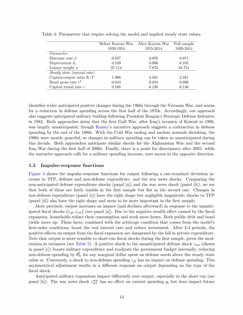
Table 4: Parameters that require solving the model and implied steady state values.
Before Korean War After Korean War Full sample1939-1954 1955-2014 1939-2014
ParameterDiscount rate β 0.957 0.976 0.971Depreciation δ1 0.109 0.096 0.105Leisure weight φ 37.114 7.873 34.751Steady state (annual rate)Capital-output ratio K/Y 1.986 2.561 2.281Bond gross rate rb 0.044 0.024 0.030Capital rental rate r 0.168 0.130 0.146
identifies wider anticipated positive changes during the 1960s through the Vietnam War, and warnsfor a reduction in defense spending across the first half of the 1970s. Accordingly, our approachalso suggests anticipated military buildup following President Reagan’s Strategic Defense Initiativein 1983. Both approaches deem that the first Gulf War, after Iraq’s invasion of Kuwait in 1990,was largely unanticipated, though Ramey’s narrative approach suggests a contraction in defensespending by the end of the 1980s. With the Cold War ending and nuclear arsenals shrinking, the1990s were mostly peaceful, so changes in military spending can be taken as unanticipated duringthis decade. Both approaches anticipate similar shocks for the Afghanistan War and the secondIraq War during the first half of 2000s. Finally, there is a point for discrepancy after 2005: whilethe narrative approach calls for a military spending increase, ours moves in the opposite direction.
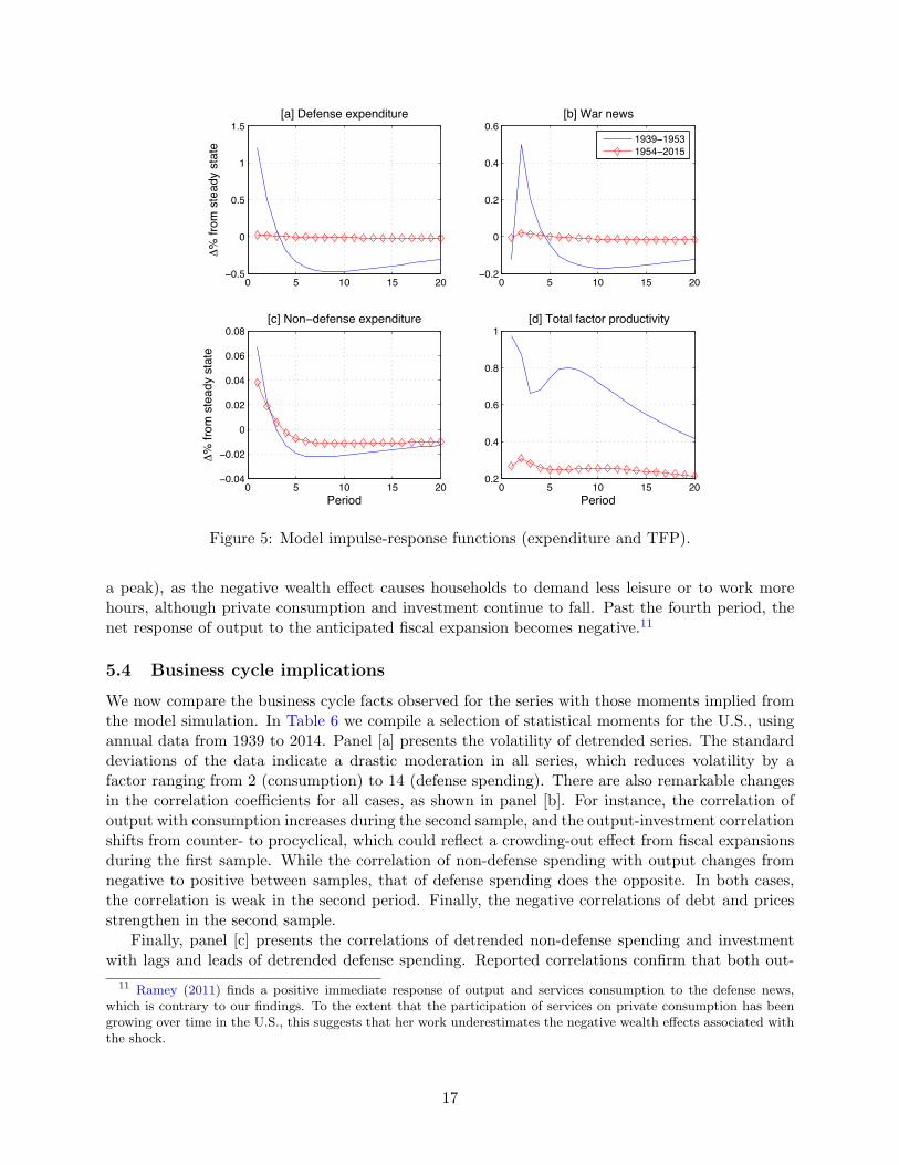
5.3 Impulse-response functions
Figure 5 shows the impulse-response functions for output following a one-standard deviation in-crease in TFP, defense and non-defense expenditure, and the war news shocks. Comparing thenon-anticipated defense expenditure shocks (panel [a]) and the war news shock (panel [b]), we seethat both of these are fairly sizable in the first sample but flat in the second one. Changes innon-defense expenditure (panel [c]) have the right shape but negligible magnitude; shocks to TFP(panel [d]) also have the right shape and seem to be more important in the first sample.
More precisely, output increases on impact (and declines afterward) in response to the unantic-ipated fiscal shocks {εgt, εmt} (see panel [a]). Due to the negative wealth effect caused by the fiscalexpansion, households reduce their consumption and work more hours. Both public debt and bondyields move up. These facts, combined with the arbitrage condition that comes from the model’sfirst-order conditions, boost the real interest rate and reduce investment. After 3-4 periods, thepositive effects on output from the fiscal expansion are dampened by the fall in private expenditure.Note that output is more sensible to short-run fiscal shocks during the first sample, given the mod-eration in variances (see Table 5). A positive shock to the unanticipated defense shock εmt (shownin panel [c]) boosts military expenditure and readjusts the government budget internally, reducingnon-defense spending by θgm for any marginal dollar spent on defense needs above the steady statevalue m. Conversely, a shock to non-defense spending εgt has no impact on defense spending. Thisasymmetrical adjustment results in a different response on output depending on the type of thefiscal shock.
Anticipated military expansions impact differently over output, especially in the short run (seepanel [b]). The war news shock εwarmt has no effect on current spending gt but does impact future
14
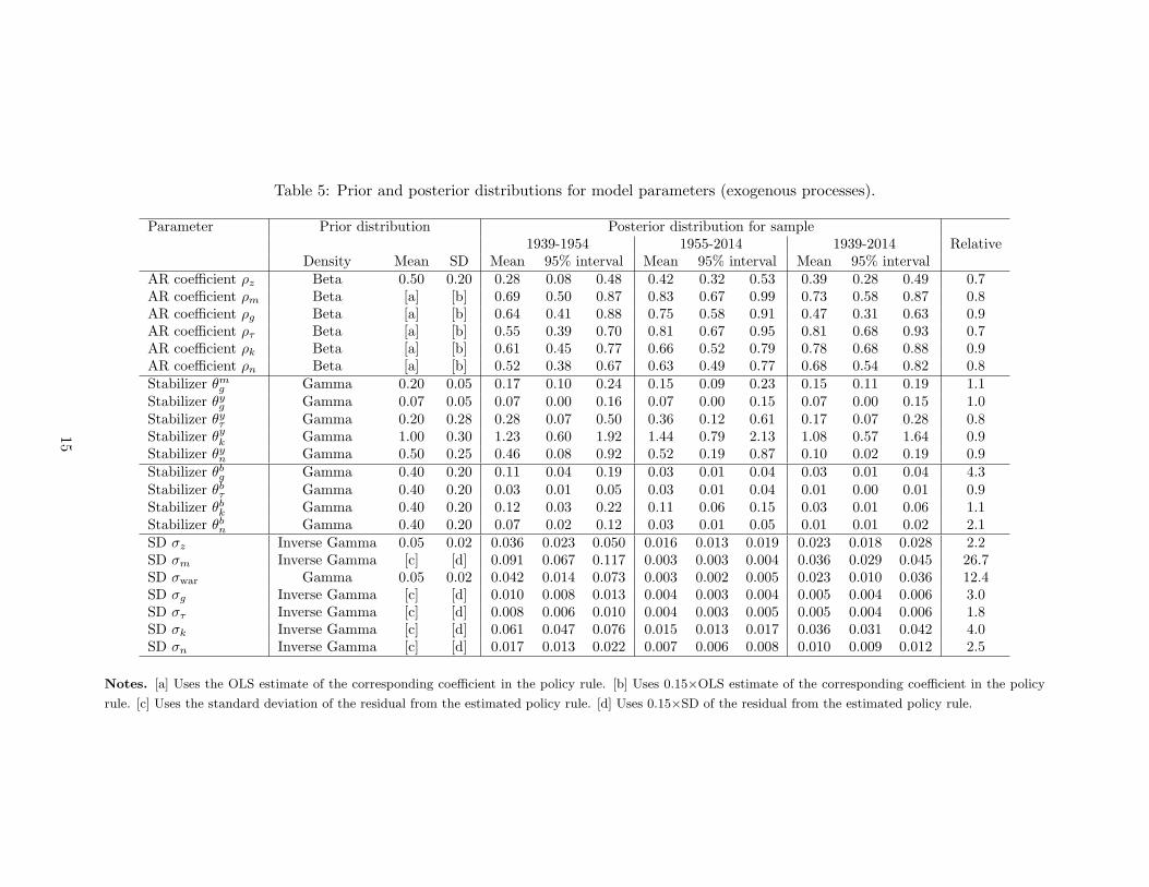
Table 5: Prior and posterior distributions for model parameters (exogenous processes).
Parameter Prior distribution Posterior distribution for sample1939-1954 1955-2014 1939-2014 Relative
Density Mean SD Mean 95% interval Mean 95% interval Mean 95% intervalAR coefficient ρz Beta 0.50 0.20 0.28 0.08 0.48 0.42 0.32 0.53 0.39 0.28 0.49 0.7AR coefficient ρm Beta [a] [b] 0.69 0.50 0.87 0.83 0.67 0.99 0.73 0.58 0.87 0.8AR coefficient ρg Beta [a] [b] 0.64 0.41 0.88 0.75 0.58 0.91 0.47 0.31 0.63 0.9AR coefficient ρτ Beta [a] [b] 0.55 0.39 0.70 0.81 0.67 0.95 0.81 0.68 0.93 0.7AR coefficient ρk Beta [a] [b] 0.61 0.45 0.77 0.66 0.52 0.79 0.78 0.68 0.88 0.9AR coefficient ρn Beta [a] [b] 0.52 0.38 0.67 0.63 0.49 0.77 0.68 0.54 0.82 0.8Stabilizer θmg Gamma 0.20 0.05 0.17 0.10 0.24 0.15 0.09 0.23 0.15 0.11 0.19 1.1Stabilizer θyg Gamma 0.07 0.05 0.07 0.00 0.16 0.07 0.00 0.15 0.07 0.00 0.15 1.0Stabilizer θyτ Gamma 0.20 0.28 0.28 0.07 0.50 0.36 0.12 0.61 0.17 0.07 0.28 0.8Stabilizer θyk Gamma 1.00 0.30 1.23 0.60 1.92 1.44 0.79 2.13 1.08 0.57 1.64 0.9Stabilizer θyn Gamma 0.50 0.25 0.46 0.08 0.92 0.52 0.19 0.87 0.10 0.02 0.19 0.9Stabilizer θbg Gamma 0.40 0.20 0.11 0.04 0.19 0.03 0.01 0.04 0.03 0.01 0.04 4.3Stabilizer θbτ Gamma 0.40 0.20 0.03 0.01 0.05 0.03 0.01 0.04 0.01 0.00 0.01 0.9Stabilizer θbk Gamma 0.40 0.20 0.12 0.03 0.22 0.11 0.06 0.15 0.03 0.01 0.06 1.1Stabilizer θbn Gamma 0.40 0.20 0.07 0.02 0.12 0.03 0.01 0.05 0.01 0.01 0.02 2.1SD σz Inverse Gamma 0.05 0.02 0.036 0.023 0.050 0.016 0.013 0.019 0.023 0.018 0.028 2.2SD σm Inverse Gamma [c] [d] 0.091 0.067 0.117 0.003 0.003 0.004 0.036 0.029 0.045 26.7SD σwar Gamma 0.05 0.02 0.042 0.014 0.073 0.003 0.002 0.005 0.023 0.010 0.036 12.4SD σg Inverse Gamma [c] [d] 0.010 0.008 0.013 0.004 0.003 0.004 0.005 0.004 0.006 3.0SD στ Inverse Gamma [c] [d] 0.008 0.006 0.010 0.004 0.003 0.005 0.005 0.004 0.006 1.8SD σk Inverse Gamma [c] [d] 0.061 0.047 0.076 0.015 0.013 0.017 0.036 0.031 0.042 4.0SD σn Inverse Gamma [c] [d] 0.017 0.013 0.022 0.007 0.006 0.008 0.010 0.009 0.012 2.5
Notes. [a] Uses the OLS estimate of the corresponding coefficient in the policy rule. [b] Uses 0.15×OLS estimate of the corresponding coefficient in the policy
rule. [c] Uses the standard deviation of the residual from the estimated policy rule. [d] Uses 0.15×SD of the residual from the estimated policy rule.
15
1939 1941 1943 1945 1947 1949 1951 1953 1954−20
−10
0
10
20
30
40
50
Year
% o
f la
st
qu
art
er’s G
DP
(a
nn
ua
l a
ve
rag
e)
Narrative approach
DSGE approach
1939 1941 1943 1945 1947 1949 1951 1953 1954−0.02
−0.01
0
0.01
0.02
0.03
0.04
0.05
Ne
ws s
ho
ck
Figure 3: News of war, narrative vs. DSGE approaches (1939-1954 sample).
1939 1950 1960 1970 1980 1990 2000 2010 2015−30
−20
−10
0
10
20
30
40
50
Year
% o
f la
st
qu
art
er’s G
DP
(a
nn
ua
l a
ve
rag
e)
World War II (1944)
Korean War (1953)
Vietnam War (1967)
Reagan buildup (1982−5)
Gulf War (1991)
War in Afghanistan (2002)
Narrative approach
DSGE approach
1939 1950 1960 1970 1980 1990 2000 2010 2015−30
−20
−10
0
10
20
30
40
50
Year
% o
f la
st
qu
art
er’s G
DP
(a
nn
ua
l a
ve
rag
e)
World War II (1944)
Korean War (1953)
Vietnam War (1967)
Reagan buildup (1982−5)
Gulf War (1991)
War in Afghanistan (2002)
Narrative approach
DSGE approach
1939 1950 1960 1970 1980 1990 2000 2010 2015−30
−20
−10
0
10
20
30
40
50
Year
% o
f la
st
qu
art
er’s G
DP
(a
nn
ua
l a
ve
rag
e)
World War II (1944)
Korean War (1953)
Vietnam War (1967)
Reagan buildup (1982−5)
Gulf War (1991)
War in Afghanistan (2002)
Narrative approach
DSGE approach
1939 1950 1960 1970 1980 1990 2000 2010 2015−0.03
−0.02
−0.01
0
0.01
0.02
0.03
0.04
0.05
Ne
ws s
ho
ck
Figure 4: News of war, narrative vs. DSGE approaches (full sample).
spending gt+1. However, given the tax rules, families discount tax burden increases that mayspread across a long horizon—due to the possibility of war. As public debt is expected to rise,the real interest rate rises as well while investment falls. The net aggregate effect is an immediatecontraction in output. In the second period, output reacts positively to the fiscal news (reaching
16
0 5 10 15 20−0.5
0
0.5
1
1.5
[a] Defense expenditure
∆%
fro
m s
teady s
tate
0 5 10 15 20−0.2
0
0.2
0.4
0.6
[b] War news
1939−1953
1954−2015
0 5 10 15 20−0.04
−0.02
0
0.02
0.04
0.06
0.08
[c] Non−defense expenditure
∆%
fro
m s
teady s
tate
Period0 5 10 15 20
0.2
0.4
0.6
0.8
1
[d] Total factor productivity
Period
Figure 5: Model impulse-response functions (expenditure and TFP).
a peak), as the negative wealth effect causes households to demand less leisure or to work morehours, although private consumption and investment continue to fall. Past the fourth period, thenet response of output to the anticipated fiscal expansion becomes negative.11
5.4 Business cycle implications
We now compare the business cycle facts observed for the series with those moments implied fromthe model simulation. In Table 6 we compile a selection of statistical moments for the U.S., usingannual data from 1939 to 2014. Panel [a] presents the volatility of detrended series. The standarddeviations of the data indicate a drastic moderation in all series, which reduces volatility by afactor ranging from 2 (consumption) to 14 (defense spending). There are also remarkable changesin the correlation coefficients for all cases, as shown in panel [b]. For instance, the correlation ofoutput with consumption increases during the second sample, and the output-investment correlationshifts from counter- to procyclical, which could reflect a crowding-out effect from fiscal expansionsduring the first sample. While the correlation of non-defense spending with output changes fromnegative to positive between samples, that of defense spending does the opposite. In both cases,the correlation is weak in the second period. Finally, the negative correlations of debt and pricesstrengthen in the second sample.
Finally, panel [c] presents the correlations of detrended non-defense spending and investmentwith lags and leads of detrended defense spending. Reported correlations confirm that both out-
11 Ramey (2011) finds a positive immediate response of output and services consumption to the defense news,which is contrary to our findings. To the extent that the participation of services on private consumption has beengrowing over time in the U.S., this suggests that her work underestimates the negative wealth effects associated withthe shock.
17
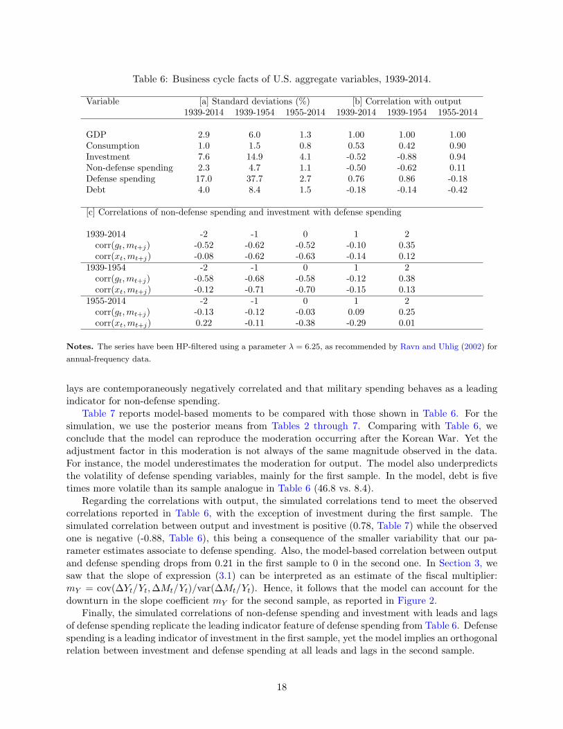
Table 6: Business cycle facts of U.S. aggregate variables, 1939-2014.
Variable [a] Standard deviations (%) [b] Correlation with output1939-2014 1939-1954 1955-2014 1939-2014 1939-1954 1955-2014
GDP 2.9 6.0 1.3 1.00 1.00 1.00Consumption 1.0 1.5 0.8 0.53 0.42 0.90Investment 7.6 14.9 4.1 -0.52 -0.88 0.94Non-defense spending 2.3 4.7 1.1 -0.50 -0.62 0.11Defense spending 17.0 37.7 2.7 0.76 0.86 -0.18Debt 4.0 8.4 1.5 -0.18 -0.14 -0.42
[c] Correlations of non-defense spending and investment with defense spending
1939-2014 -2 -1 0 1 2corr(gt,mt+j) -0.52 -0.62 -0.52 -0.10 0.35corr(xt,mt+j) -0.08 -0.62 -0.63 -0.14 0.12
1939-1954 -2 -1 0 1 2corr(gt,mt+j) -0.58 -0.68 -0.58 -0.12 0.38corr(xt,mt+j) -0.12 -0.71 -0.70 -0.15 0.13
1955-2014 -2 -1 0 1 2corr(gt,mt+j) -0.13 -0.12 -0.03 0.09 0.25corr(xt,mt+j) 0.22 -0.11 -0.38 -0.29 0.01
Notes. The series have been HP-filtered using a parameter λ = 6.25, as recommended by Ravn and Uhlig (2002) for
annual-frequency data.
lays are contemporaneously negatively correlated and that military spending behaves as a leadingindicator for non-defense spending.
Table 7 reports model-based moments to be compared with those shown in Table 6. For thesimulation, we use the posterior means from Tables 2 through 7. Comparing with Table 6, weconclude that the model can reproduce the moderation occurring after the Korean War. Yet theadjustment factor in this moderation is not always of the same magnitude observed in the data.For instance, the model underestimates the moderation for output. The model also underpredictsthe volatility of defense spending variables, mainly for the first sample. In the model, debt is fivetimes more volatile than its sample analogue in Table 6 (46.8 vs. 8.4).
Regarding the correlations with output, the simulated correlations tend to meet the observedcorrelations reported in Table 6, with the exception of investment during the first sample. Thesimulated correlation between output and investment is positive (0.78, Table 7) while the observedone is negative (-0.88, Table 6), this being a consequence of the smaller variability that our pa-rameter estimates associate to defense spending. Also, the model-based correlation between outputand defense spending drops from 0.21 in the first sample to 0 in the second one. In Section 3, wesaw that the slope of expression (3.1) can be interpreted as an estimate of the fiscal multiplier:mY = cov(∆Yt/Yt,∆Mt/Yt)/var(∆Mt/Yt). Hence, it follows that the model can account for thedownturn in the slope coefficient mY for the second sample, as reported in Figure 2.
Finally, the simulated correlations of non-defense spending and investment with leads and lagsof defense spending replicate the leading indicator feature of defense spending from Table 6. Defensespending is a leading indicator of investment in the first sample, yet the model implies an orthogonalrelation between investment and defense spending at all leads and lags in the second sample.
18
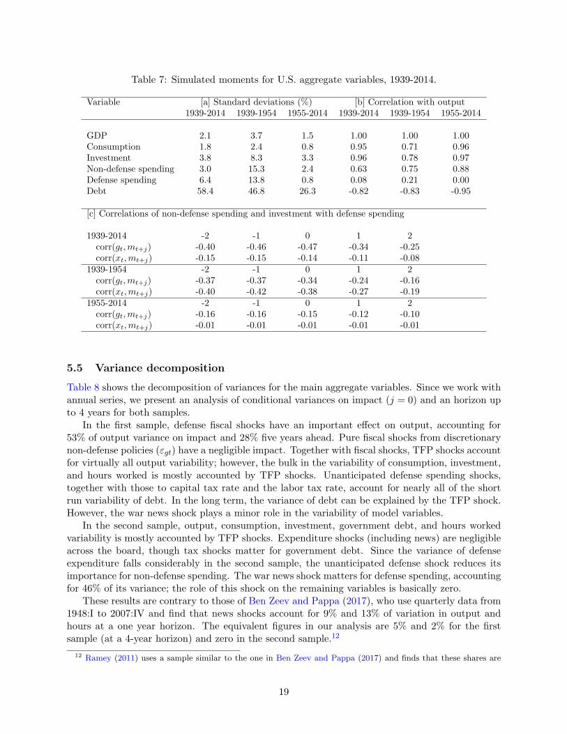
Table 7: Simulated moments for U.S. aggregate variables, 1939-2014.
Variable [a] Standard deviations (%) [b] Correlation with output1939-2014 1939-1954 1955-2014 1939-2014 1939-1954 1955-2014
GDP 2.1 3.7 1.5 1.00 1.00 1.00Consumption 1.8 2.4 0.8 0.95 0.71 0.96Investment 3.8 8.3 3.3 0.96 0.78 0.97Non-defense spending 3.0 15.3 2.4 0.63 0.75 0.88Defense spending 6.4 13.8 0.8 0.08 0.21 0.00Debt 58.4 46.8 26.3 -0.82 -0.83 -0.95
[c] Correlations of non-defense spending and investment with defense spending
1939-2014 -2 -1 0 1 2corr(gt,mt+j) -0.40 -0.46 -0.47 -0.34 -0.25corr(xt,mt+j) -0.15 -0.15 -0.14 -0.11 -0.08
1939-1954 -2 -1 0 1 2corr(gt,mt+j) -0.37 -0.37 -0.34 -0.24 -0.16corr(xt,mt+j) -0.40 -0.42 -0.38 -0.27 -0.19
1955-2014 -2 -1 0 1 2corr(gt,mt+j) -0.16 -0.16 -0.15 -0.12 -0.10corr(xt,mt+j) -0.01 -0.01 -0.01 -0.01 -0.01
5.5 Variance decomposition
Table 8 shows the decomposition of variances for the main aggregate variables. Since we work withannual series, we present an analysis of conditional variances on impact (j = 0) and an horizon upto 4 years for both samples.
In the first sample, defense fiscal shocks have an important effect on output, accounting for53% of output variance on impact and 28% five years ahead. Pure fiscal shocks from discretionarynon-defense policies (εgt) have a negligible impact. Together with fiscal shocks, TFP shocks accountfor virtually all output variability; however, the bulk in the variability of consumption, investment,and hours worked is mostly accounted by TFP shocks. Unanticipated defense spending shocks,together with those to capital tax rate and the labor tax rate, account for nearly all of the shortrun variability of debt. In the long term, the variance of debt can be explained by the TFP shock.However, the war news shock plays a minor role in the variability of model variables.
In the second sample, output, consumption, investment, government debt, and hours workedvariability is mostly accounted by TFP shocks. Expenditure shocks (including news) are negligibleacross the board, though tax shocks matter for government debt. Since the variance of defenseexpenditure falls considerably in the second sample, the unanticipated defense shock reduces itsimportance for non-defense spending. The war news shock matters for defense spending, accountingfor 46% of its variance; the role of this shock on the remaining variables is basically zero.
These results are contrary to those of Ben Zeev and Pappa (2017), who use quarterly data from1948:I to 2007:IV and find that news shocks account for 9% and 13% of variation in output andhours at a one year horizon. The equivalent figures in our analysis are 5% and 2% for the firstsample (at a 4-year horizon) and zero in the second sample.12
12 Ramey (2011) uses a sample similar to the one in Ben Zeev and Pappa (2017) and finds that these shares are
19
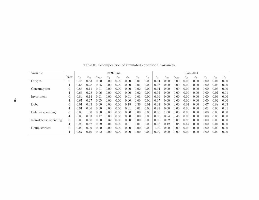
Table 8: Decomposition of simulated conditional variances.
Variable 1939-1954 1955-2014Year εz εm εwar εg ετ εk εn εc εz εm εwar εg ετ εk εn εc
Output 0 0.45 0.53 0.00 0.00 0.00 0.00 0.01 0.00 0.94 0.00 0.00 0.02 0.00 0.00 0.04 0.004 0.66 0.28 0.05 0.00 0.00 0.00 0.01 0.00 0.97 0.00 0.00 0.00 0.00 0.00 0.03 0.00
Consumption 0 0.86 0.11 0.01 0.00 0.00 0.00 0.02 0.00 0.94 0.00 0.00 0.00 0.00 0.00 0.06 0.004 0.63 0.28 0.06 0.00 0.00 0.00 0.02 0.00 0.92 0.00 0.00 0.00 0.00 0.00 0.07 0.01
Investment 0 0.84 0.14 0.01 0.00 0.00 0.01 0.01 0.00 0.96 0.00 0.00 0.00 0.00 0.00 0.03 0.004 0.67 0.27 0.05 0.00 0.00 0.00 0.00 0.00 0.97 0.00 0.00 0.00 0.00 0.00 0.02 0.00
Debt 0 0.01 0.43 0.00 0.00 0.00 0.18 0.36 0.01 0.02 0.00 0.00 0.01 0.00 0.07 0.88 0.034 0.91 0.06 0.00 0.00 0.00 0.01 0.01 0.00 0.92 0.00 0.00 0.00 0.00 0.01 0.06 0.01
Defense spending 0 0.00 1.00 0.00 0.00 0.00 0.00 0.00 0.00 0.00 1.00 0.00 0.00 0.00 0.00 0.00 0.004 0.00 0.83 0.17 0.00 0.00 0.00 0.00 0.00 0.00 0.54 0.46 0.00 0.00 0.00 0.00 0.00
Non-defense spending 0 0.00 0.68 0.00 0.32 0.00 0.00 0.00 0.00 0.00 0.02 0.00 0.98 0.00 0.00 0.00 0.004 0.23 0.62 0.09 0.04 0.00 0.01 0.01 0.00 0.08 0.12 0.08 0.67 0.00 0.00 0.04 0.00
Hours worked 0 0.90 0.09 0.00 0.00 0.00 0.00 0.00 0.00 1.00 0.00 0.00 0.00 0.00 0.00 0.00 0.004 0.87 0.10 0.02 0.00 0.00 0.00 0.00 0.00 0.99 0.00 0.00 0.00 0.00 0.00 0.00 0.00
20
5.6 Expenditure multipliers
As we show below, the definition of the multiplier is critical for its magnitude. We distinguish be-tween present-value multipliers (Mountford and Uhlig 2009) and peak impact multipliers (Blanchardand Perotti 2002 and many others). We find that the former definition cannot yield multipliersabove unity, but the latter can.13
Present value multipliers Following Mountford and Uhlig (2009), we now display present-valuemultipliers. Let ∆yt+i and ∆gst+i denote the impulse-responses of output and government spending(here gs = {g,m}) with respect to fiscal shock εgt or εmt. The present value multiplier generatedby a change in the present value of government spending gs over a j-period horizon is
PV ygs(j) =
∑ji=0∆yt+i ×
∏ji=0 r
−1b,t+i
∑ji=0∆gst+i ×
∏ji=0 r
−1b,t+i
·y
gs, (5.1)
where rb,t+i represents the impulse-response for the bond yield. The multipliers for consumption,investment, non-defense, and defense expenditure are defined accordingly.
Table 9 shows the present value multipliers implied by our model, where we look at both samplesand an horizon up to 4 years. For time horizon j = 0, the multiplier is measured on impact. Asthese multipliers are calculated using the impulse-response functions derived from our structuralDSGE model, the estimate of the multiplier cannot be contaminated by an identification bias.When considering the multiplier implied by defense spending, gs = m, the fiscal adjustment takingplace within government budget (parameter θmg in equation [4.10]) is internalized into the model: apositive fiscal shock εmt boosts defense spending over its steady value m, prompting the governmentto adjust non-defense spending by −θmg .
From Table 9 we draw three conclusions. First, the output present-value multipliers are alwaysbelow unity and the consumption and investment multipliers are negative, consistent with crowdingout.14 Moreover, there are not substantial differences between both periods. The multiplier of non-defense spending has a modest increase and the defense spending multiplier has a modest decrease.Second, non-defense multipliers are slightly higher than defense ones, a result from the asymmetricbudgetary adjustment motivated by θmg . The values of PV g
m show that a change in military spendingis not a free lunch in terms of non-defense outlays, especially during the second sample. Finally,the value of the multiplier decreases as the time horizon increases.
The posterior distributions in Table 3 show three key parameters that change in the secondsample: the Frisch elasticity of labor supply 1/χ (falls), the habit persistence parameter µ, and thecapital adjustment cost κ (both increase). These changes can moderate the response of output whenaffected by fiscal shocks: a more inelastic labor supply cushions the change in hours worked when thehousehold observes a negative income effect due to higher government spending. Similarly, the othertwo parameters induce a higher real rigidity in both consumption (when µ increases, householdssmooth consumption plans), and investment (when κ increases, firms find costlier adjusting capital).However, the multipliers reported in Table 9 indicate that these changes are rather small.
Finally, changes in the fiscal rule volatilities, as shown in Table 5, are unlikely to have alteredfiscal multipliers. The moderation in the structural standard deviations are neutral according to(5.1), given that they increase its numerator and denominator by same scale.15
2% (ouptut) and 4% (hours).13 This issue has also been raised by Zubairy (2014) and Ramey and Zubairy (2018).14 The inability of the neoclassical framework to produce large multipliers has been highlighted by Dyrda and Rıos-
Rull (2012) and Rıos-Rull and Huo (2013), who suggest introducing other frictions to motivate higher multipliers.15 For the rest of fiscal parameters in Table 5, it is not straightforward to infer the effects they produce on the
21
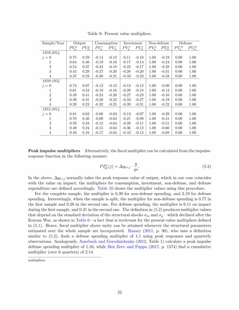
Table 9: Present value multipliers.
Sample/Year Output Consumption Investment Non-defense DefensePV y
g PV ym PV c
g PV cm PV x
g PV xm PV g
g PV gm PV m
g PV mm
1939-2014j = 0 0.75 0.59 -0.14 -0.12 -0.11 -0.10 1.00 -0.19 0.00 1.00j = 1 0.64 0.46 -0.19 -0.16 -0.17 -0.14 1.00 -0.24 0.00 1.00j = 2 0.54 0.37 -0.24 -0.18 -0.22 -0.17 1.00 -0.28 0.00 1.00j = 3 0.45 0.29 -0.27 -0.20 -0.28 -0.20 1.00 -0.31 0.00 1.00j = 4 0.37 0.23 -0.30 -0.21 -0.33 -0.23 1.00 -0.33 0.00 1.001939-1954j = 0 0.74 0.67 -0.13 -0.12 -0.13 -0.12 1.00 -0.09 0.00 1.00j = 1 0.61 0.53 -0.19 -0.16 -0.20 -0.18 1.00 -0.13 0.00 1.00j = 2 0.49 0.41 -0.24 -0.20 -0.27 -0.23 1.00 -0.16 0.00 1.00j = 3 0.39 0.31 -0.28 -0.22 -0.33 -0.27 1.00 -0.19 0.00 1.00j = 4 0.29 0.23 -0.32 -0.25 -0.39 -0.31 1.00 -0.22 0.00 1.001955-2014j = 0 0.81 0.62 -0.06 -0.03 -0.13 -0.07 1.00 -0.29 0.00 1.00j = 1 0.70 0.46 -0.09 -0.04 -0.21 -0.09 1.00 -0.41 0.00 1.00j = 2 0.59 0.34 -0.12 -0.04 -0.29 -0.11 1.00 -0.51 0.00 1.00j = 3 0.49 0.24 -0.15 -0.04 -0.36 -0.12 1.00 -0.60 0.00 1.00j = 4 0.40 0.16 -0.17 -0.04 -0.43 -0.12 1.00 -0.68 0.00 1.00
Peak impulse multipliers Alternatively, the fiscal multiplier can be calculated from the impulse-response function in the following manner:
PIygs(j) = ∆yt+j ·y
gs. (5.2)
In the above, ∆yt+j normally takes the peak response value of output, which in our case coincideswith the value on impact; the multipliers for consumption, investment, non-defense, and defenseexpenditure are defined accordingly. Table 10 shows the multiplier values using this procedure.
For the complete sample, the multiplier is 0.39 for non-defense spending, and 2.19 for defensespending. Interestingly, when the sample is split, the multiplier for non-defense spending is 0.77 inthe first sample and 0.28 in the second one. For defense spending, the multiplier is 6.11 on impactduring the first sample, and 0.21 in the second one. The definition in (5.2) produces multiplier valuesthat depend on the standard deviation of the structural shocks σm and σg—which declined after theKorean War, as shown in Table 6—a fact that is irrelevant for the present-value multipliers definedin (5.1). Hence, fiscal multiplier above unity can be attained whenever the structural parametersestimated over the whole sample are incorporated. Ramey (2011, p. 30), who uses a definitionsimilar to (5.2), finds a defense spending multiplier of 1.1 using peak responses and quarterlyobservations. Analogously, Auerbach and Gorodnichenko (2012, Table 1) calculate a peak impulsedefense spending multiplier of 1.16, while Ben Zeev and Pappa (2017, p. 1574) find a cumulativemultiplier (over 6 quarters) of 2.14.
multipliers.
22
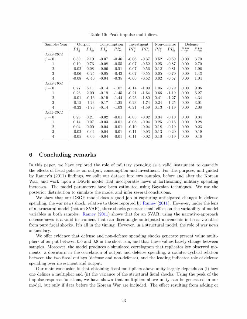
Table 10: Peak impulse multipliers.
Sample/Year Output Consumption Investment Non-defense DefensePIyg PIym PIcg PIcm PIxg PIxm PIgg PIgm PImg PImm
1939-2014j = 0 0.39 2.19 -0.07 -0.46 -0.06 -0.37 0.52 -0.69 0.00 3.70j = 1 0.10 0.76 -0.08 -0.55 -0.07 -0.52 0.25 -0.87 0.00 2.70j = 2 -0.02 0.08 -0.06 -0.51 -0.07 -0.56 0.12 -0.81 0.00 1.96j = 3 -0.06 -0.25 -0.05 -0.43 -0.07 -0.55 0.05 -0.70 0.00 1.43j = 4 -0.08 -0.40 -0.04 -0.35 -0.06 -0.52 0.02 -0.57 0.00 1.041939-1954j = 0 0.77 6.11 -0.14 -1.07 -0.14 -1.09 1.05 -0.79 0.00 9.06j = 1 0.26 2.00 -0.19 -1.45 -0.21 -1.64 0.66 -1.19 0.00 6.27j = 2 -0.01 -0.16 -0.19 -1.44 -0.23 -1.80 0.41 -1.27 0.00 4.34j = 3 -0.15 -1.23 -0.17 -1.25 -0.23 -1.74 0.24 -1.25 0.00 3.01j = 4 -0.22 -1.73 -0.14 -1.03 -0.21 -1.59 0.13 -1.19 0.00 2.081955-2014j = 0 0.28 0.21 -0.02 -0.01 -0.05 -0.02 0.34 -0.10 0.00 0.34j = 1 0.14 0.07 -0.03 -0.01 -0.08 -0.04 0.25 -0.16 0.00 0.28j = 2 0.04 0.00 -0.04 -0.01 -0.10 -0.04 0.18 -0.19 0.00 0.23j = 3 -0.02 -0.04 -0.04 -0.01 -0.11 -0.03 0.13 -0.20 0.00 0.19j = 4 -0.05 -0.06 -0.04 -0.01 -0.11 -0.02 0.10 -0.19 0.00 0.16
6 Concluding remarks
In this paper, we have explored the role of military spending as a valid instrument to quantifythe effects of fiscal policies on output, consumption and investment. For this purpose, and guidedby Ramey’s (2011) findings, we split our dataset into two samples, before and after the KoreanWar, and work upon a DSGE model that incorporates news of forthcoming military spendingincreases. The model parameters have been estimated using Bayesian techniques. We use theposterior distribution to simulate the model and infer several conclusions.
We show that our DSGE model does a good job in capturing anticipated changes in defensespending, the war news shock, relative to those reported by Ramey (2011). However, under the lensof a structural model (not an SVAR), these shocks generate small effect on the variability of modelvariables in both samples. Ramey (2011) shows that for an SVAR, using the narrative-approachdefense news is a valid instrument that can disentangle anticipated movements in fiscal variablesfrom pure fiscal shocks. It’s all in the timing. However, in a structural model, the role of war newsis ancillary.
We offer evidence that defense and non-defense spending shocks generate present value multi-pliers of output between 0.6 and 0.8 in the short run, and that these values barely change betweensamples. Moreover, the model produces a simulated correlogram that replicates key observed mo-ments: a downturn in the correlation of output and defense spending, a counter-cyclical relationbetween the two fiscal outlays (defense and non-defense), and the leading indicator role of defensespending over investment and output.
Our main conclusion is that obtaining fiscal multipliers above unity largely depends on (i) howone defines a multiplier and (ii) the variance of the structural fiscal shocks. Using the peak of theimpulse-response functions, we have shown that multipliers above unity can be generated in ourmodel, but only if data before the Korean War are included. The effect resulting from adding or
23

subtracting these years follows the large moderation that took place after WWII and the KoreanWar, particularly affecting military spending. Hence, multipliers that include data from these yearsare to a large extent influenced by these observations. Once we get rid of these data points, themodel is unable to produce multipliers above unity, regardless of the definition adopted. For thisreason, we recommend using the concept of present value multiplier proposed by Mountford andUhlig (2009), given that it is neutral with respect to the variance of the structural fiscal shocks. Aswe claim in the title of our paper, it’s all in the variances.
References
Alan Auerbach and Yuriy Gorodnichenko. Measuring the output responses to fiscal policy. AmericanEconomic Journal: Economic Policy, 4(2):1–27, 2012.
Robert Barro and Charles Redlick. Macroeconomic effects from government purchases and taxes.Quarterly Journal of Economics, 126(1):51–102, 2011.
Robert Barsky and Eric Sims. News shocks and business cycles. Journal of Monetary Economics,58:273–89, 2011.
Paul Beaudry and Franck Portier. An exploration into Pigou’s theory of cycles. Journal of MonetaryEconomics, 51(6):1183–216, 2004.
Paul Beaudry and Franck Portier. When can changes in expectations cause business cycle fluctua-tions in neo-classical settings? Journal of Economic Theory, 135(1):458–77, 2007.
Nadav Ben Zeev and Evi Pappa. Multipliers of unexpected increases in defense spending: anempirical investigation. Journal of Economic Dynamics and Control, 57:205–26, 2015.
Nadav Ben Zeev and Evi Pappa. Chronicle of a war foretold: the macroeconomic effects of antici-pated defense spending shocks. The Economic Journal, 127(603):1568–97, 2017.
Olivier Blanchard and Roberto Perotti. An empirical characterization of the dynamic effects ofchanges in government spending and taxes on output. Quarterly Journal of Economics, 117(4):1329–68, 2002.
Benjamin Born, Alexandra Peter, and Johannes Pfeifer. Fiscal news and macroeconomic volatility.Journal of Economic Dynamics and Control, 37(12):2582–601, 2013.
Thomas Chadefaux. Early warning signals for war in the news. Journal of Peace Research, 51(1):5–18, 2014.
Thomas Chadefaux. Market anticipations of conflict onsets. Journal of Peace Research, 54(2):313–27, 2017.
Raj Chetty, Adam Guren, Day Manoli, and Andrea Weber. Are micro and macro labor supplyelasticities consistent? A review evidence on the intensive and extensive margins. AmericanEconomic Review, 101(3):471–5, 2011.
John Cogan, Tobias Cwik, John Taylor, and Volker Wieland. New Keynesian versus old Keynesiangovernment spending multipliers. Journal of Economic Dynamics and Control, 34:281–95, 2010.
24
Sebastian Dyrda and Jose-Vıctor Rıos-Rull. Models of government expenditure multipliers. Eco-nomic Policy Paper 12-2, Federal Reserve Bank of Minneapolis, 2012.
Jesus Fernandez-Villaverde, Pablo Guerron-Quintana, Keith Kuester, and Juan Rubio-Ramırez.Fiscal volatility shocks and economic activity. American Economic Review, 105(11):3352–84,2015.
Jordi Galı, David Lopez-Salido, and Javier Valles. Understanding the effects of government spendingon consumption. Journal of the European Economic Association, 5(1):227–70, 2007.
John Geweke. Complete and Incomplete Econometric Models. Princeton University Press, Prince-ton, NJ, 2010.
George Hall. Exchange rates and causalities during the First World War. Journal of MonetaryEconomics, 51(8):1711–42, 2004.
Robert Hall. By how much does GDP rise if the government buys more output? Brookings Paperson Economic Activity, 2:183–231, 2009.
Jonathan Heathcote, Kjetil Storesletten, and Gianluca Violante. The macroeconomic implicationsof rising wage inequality in the United States. Journal of Political Economy, 118(4):681–722,2010.
Eric Leeper, Michael Plante, and Nora Traum. Dynamics of fiscal financing in the United States.Journal of Econometrics, 156(2):304–21, 2010.
Eric Leeper, Nora Traum, and Todd Walker. Clearing up the fiscal multiplier morass. AmericanEconomic Review, 107(8):2409–54, 2017.
Enrique Mendoza, Assaf Razin, and Linda Tesar. Effective tax rates in macroeconomics: Cross-country estimates of tax rates on factor incomes and consumption. Journal of Monetary Eco-nomics, 34(3):297–323, 1994.
Karel Mertens and Morten Ravn. Understanding the aggregate effects of anticipated and unantic-ipated tax policy shocks. Review of Economic Dynamics, 14(1):27–54, 2011.
Andrew Mountford and Harald Uhlig. What are the effects of fiscal policy shocks? Journal ofApplied Econometrics, 24(6):960–92, 2009.
Hannes Mueller and Christopher Rauh. Reading between the lines: predictions of political violenceusing newspaper text. Working Paper 990, Barcelona Graduate School of Economics, 2017.
Lee Ohanian. The macroeconomic effects of war finance in the United States: World War II andthe Korean War. American Economic Review, 87(1):23–40, 1997.
Roberto Perotti. In search of the transmission mechanism of fiscal policy. In NBER MacroeconomicsAnnual 2007, volume 22, pages 169–226. National Bureau of Economic Research, 2008.
Valerie Ramey. Defense news shocks, 1939-2008: an analysis based on news sources. Unpublishedmanuscript, 2009.
Valerie Ramey. Identifying government spending shocks: It’s all in the timing. Quarterly Journalof Economics, 126(1):1–50, 2011.
25
Valerie Ramey and Sarah Zubairy. Government spending multipliers in good times and in bad:evidence from US historical data. Journal of Political Economy, 126(2):850–901, 2018.
Morten Ravn and Harald Uhlig. On adjusting the Hodrick-Prescott filter for the frequency ofobservations. Review of Economics and Statistics, 84(2):371–80, 2002.
Morten Ravn, Stephanie Schmitt-Grohe, and Martın Uribe. Deep habits. Review of EconomicStudies, 73(1):195–218, 2006.
Roberto Rigobon and Brian Sack. The effects of war risk on U.S. financial markets. Journal ofBanking and Finance, 29(7):1769–89, 2005.
Jose-Vıctor Rıos-Rull and Zhen Huo. A realistic neoclassical multiplier. Economic Policy Paper13-5, Federal Reserve Bank of Minneapolis, 2013.
Stephanie Schmitt-Grohe and Martın Uribe. What’s news in business cycles. Econometrica, 80(6):2733–64, 2012.
Frank Smets and Rafael Wouters. Shocks and frictions in US business cycles: a Bayesian DSGEapproach. American Economic Review, 97(3):586–606, 2007.
Antonio Spilimbergo, Steve Symansky, and Martin Schindler. Fiscal multipliers. IMF Staff PositionNote SPN/09/11, International Monetary Fund, 2009.
Sarah Zubairy. On fiscal multipliers: estimates from a medium scale DSGE model. InternationalEconomic Review, 55(1):169–95, 2014.
A Data appendix
Aggregate series come from the Bureau of Economic Analysis (BEA). Given our interest to incor-porate observations that include WWII, our analysis is limited to annual series, as quarterly seriesare only provided by the BEA from 1947 to present. Nominal series are transformed into real seriesby dividing by the GDP implicit deflator (line 1 Table 1.1.4).
Consumption Consumption C is defined as the sum of non durable goods consumption plusservices consumption, CNonDur + CServ (lines 5 and 6 at Table 1.1.5).
Investment Investment X is defined as the sum of durable goods consumption plus gross privatedomestic investment, CDur +GPDI (lines 4 and 7 at Table 1.1.5).
Government expenditure Total government expenditure is divided into non-defense govern-ment expenditure G and defense government expenditure M . Non-defense expenditure consists offederal spending plus state and local public expenditure (Table 1.1.5, lines 25 and 26). Defensegovernment expenditure M is retrieved from Table 1.1.5, line 24. The series of defense governmentexpenditures spans from 1929 through 2014. Table 1.1.6 uses different deflators for governmentspendings: from 1929 to 1947, from 1942 to 1962, from 1962 to 1982, from 1982 to 2002, and from2000 to 2014. For the overlapping years, we take the average of the two measures of the two changes(Hall 2009).
26
Tax rates We follow the methodology proposed by Mendoza, Razin, and Tesar (1994), who deriveaggregate estimates for effective tax rates using national accounts.
The consumption tax rate is computed as the sum of Excise taxes, ExcT , Customs duties,CustDut, and Sales taxes, SalesT , divided by the sum of Personal consumption expenditures Cand total government expenditures G + M (lines 5, 6, and 7 from Table 3.2 and Lines 2 and 22from Table 1.1.5):
τc =ExcT + CustDut+ SalesT
C + (G+M).
The income tax rate is calculated as the ratio of Income tax revenues IncT (federal, state, andlocal, Lines 3 and 9 in Table 3.4) over the sum of Proprietors’ income with inventory valuation andcapital consumption adjustments (PI, Line 9 in Table 2.1), Rental income of persons with capitalconsumption adjustment (RICCA, Line 12 in Table 2.1), Personal income receipts on assets (PIRA,Line 13 in Table 2.1), Wages and salaries (W ) and Supplements to wages and salaries (SW ) (Lines3 and 6 in Table 2.1):
τY =IncT
PI +RICCA+ PIRA+ (W + SW ).
Using the calculated tax rate on income τY , the tax rate on labor income τn is derived as
τn =
(
τY +GSI
W + SW
)
W + SW
CE.
where GSI denotes Contributions for government social insurance (Line 7 in Table 3.1), and CEdenotes Compensation of employees (Line 2 in Table 2.1).
The tax rate on capital income is computed as follows:
τk =τY (PI +RICCA+ PIRA) + PT + TCI
PI + PIRA+ IRA,
where PT denotes Property taxes (Line 11 in Table 3.4), TCI denotes taxes on corporate income(Lines 7 and 10 in Table 3.2), and IRA denotes Income receipts on assets (Line 9 in Table 4.1).
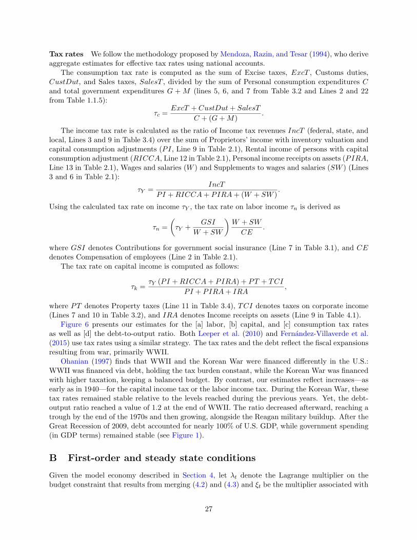
Figure 6 presents our estimates for the [a] labor, [b] capital, and [c] consumption tax ratesas well as [d] the debt-to-output ratio. Both Leeper et al. (2010) and Fernandez-Villaverde et al.(2015) use tax rates using a similar strategy. The tax rates and the debt reflect the fiscal expansionsresulting from war, primarily WWII.
Ohanian (1997) finds that WWII and the Korean War were financed differently in the U.S.:WWII was financed via debt, holding the tax burden constant, while the Korean War was financedwith higher taxation, keeping a balanced budget. By contrast, our estimates reflect increases—asearly as in 1940—for the capital income tax or the labor income tax. During the Korean War, thesetax rates remained stable relative to the levels reached during the previous years. Yet, the debt-output ratio reached a value of 1.2 at the end of WWII. The ratio decreased afterward, reaching atrough by the end of the 1970s and then growing, alongside the Reagan military buildup. After theGreat Recession of 2009, debt accounted for nearly 100% of U.S. GDP, while government spending(in GDP terms) remained stable (see Figure 1).
B First-order and steady state conditions
Given the model economy described in Section 4, let λt denote the Lagrange multiplier on thebudget constraint that results from merging (4.2) and (4.3) and ξt be the multiplier associated with
27
1930 1950 1970 1990 20150
0.05
0.1
0.15
0.2
0.25
[a] Labor income tax rate
Pe
rce
nt
of
GD
P
1930 1950 1970 1990 20150
0.1
0.2
0.3
0.4
0.5
[b] Capital income tax rate
1930 1950 1970 1990 20150.01
0.02
0.03
0.04
0.05
0.06
0.07
[c] Consumption tax rate
Year
Pe
rce
nt
of
GD
P
1930 1950 1970 1990 20150
0.2
0.4
0.6
0.8
1
1.2
1.4
[d] Debt−to−GDP ratio
Year
Figure 6: Selected fiscal variables, 1930-2015.
the law of motion for capital (4.4). Then, the first-order conditions that characterize householdequilibrium are given by the derivatives of the household Lagrangian with respect to consumption,investment, hours worked, utilization, capital, and bonds
λt(1 + τct) = q−1t − βµEtq
−1t+1
λt = ξt − ξt
[
S′
(
xtxt−1
)
xtxt−1
+ S
(
xtxt−1
)]
+ βEtξt+1S′
(
xt+1
xt
)(
xt+1
xt
)2
λt(1− τnt)wt = φnχt
λt(1− τkt)rt = ξtδ′(ut)
ξt = βEtλt+1[(1− τk,t+1)rt+1ut+1 + δ0τk,t+1] + βEtξt+1(1− δ(ut+1))
λt = βEtλt+1rbt+1,
where qt ≡ ct−µct−1. To the equations above we add the budget constraint (4.2), the tax equation(4.3), and the law of motion for capital (4.4). For the firm, we provide a definition for output ytand take the derivatives of the profit function with respect to capital and labor inputs:
yt = AztKαFtn
1−αFt
αyt = rtKFt
(1− α)yt = wtnFt
Finally, the government needs to satisfy its budget constraint (4.8) and the fiscal rules (4.9)-(4.14).Note that combining the household and government budget constraints we get the aggregate feasi-bility constraint (4.15) and that in an equilibrium, KFt = utkt and nFt = nt.
28
In the steady state, we let y = u = z = 1. The equilibrium conditions become
λ(1 + τc) = (1− βµ)q−1
λ = ξ
λ(1− τn)w = φnχ
λ(1− τk)r = ξδ1
ξ = βλ[(1− τk)r + δ0τk] + βξ(1− δ0)
1 = βrb
1 = c+ x+ g +m
k = (1− δ0)k + x
q = (1− µ)c
1 = Akαn1−α
α = rk
(1− α) = wn.
29