DeepCloud: Detecting and Classifying Clouds in Satellite Imagery

by

Joshua Tanke

A THESIS

Presented to the Department of Computer and Information Science

of the University of Oregon in partial fulfillment of the requirements

for the degree of Bachelor of Science

June 2019

© 2019 Joshua Tanke

Abstract Detecting and classifying images of clouds at the pixel level is a crucial operation when

working with satellite imagery. The presence of clouds will distort the data across all wavelengths, and unclassified clouds over extended periods of time will render any conclusions drawn from the data useless. The type of cloud (opaque, cirrus, etc.) is also important as different types of clouds will distort the data is different ways. Many methods have been proposed to detect and classify clouds in satellite images, but they all come short of the consistent performance needed to be used in many industry applications. This paper will present a deep learning approach to detecting and classifying cloud types. Simple dense neural networks on single pixels have been tested by others and have shown improvements over previous methods of cloud detection. We will be exploring the use of time-series analysis when detecting the clouds, rather than only referencing a single image, to show how previous values of a given pixel can help improve model performance. Our experiments show that including time-series information can improve robustness when detecting and classifying clouds, especially on cloud shadows and cirrus clouds.

Acknowledgments I would like to thank Professor Stephen Fickas for his invaluable guidance and feedback during this thesis, and also for being the one who first introduced me to machine learning. His teaching fostered my fascination in getting computers to learn and gave me the tools to go out and explore the domain further. I would also like to thank the team at Google[X] for providing the satellite data used during these experiments, and specifically my manager Jie Yang for discussing the tradeoffs between various models I proposed. Lastly, thank you to all of my friends and family who have supported me throughout my time at the University of Oregon and through the process of this thesis.

Contents Introduction 1

Background Information 1 Feedforward (Dense) Neural Networks 1 Recurrent Neural Networks 2 Convolutional Neural Network 4 Normalization 5 Dropout 7 Skip Connections 7 Sentinel-2 Satellite 8

Related Prior Work 9

A New LSTM Approach 10

Dataset 10 Data Collection and Split 10 Dataset Example 11

Model Architecture & Methods 11 Data Preprocessing 11 Fully Connected Model (Baseline) 11 Fully Connected Model with LSTM Embedding 12

Results 13

Conclusions 14

Future Work 14

Bibliography 16

1

Introduction The use of remote sensing in industry applications has skyrocketed over the last decade.

With the rise of deep learning, models are able to digest large amounts of information, and industry researchers have turned to large-scale remote sensing, such as satellite imagery, to feed these models. One example of this is Planet Labs, which has received over $384M in funding to launch high-res, high-frequency satellites into orbit to support data science projects in many sectors, such as agriculture, energy, and transport [6]. A major blockage encountered when applying satellite imagery to an industry problem is that current cloud masks are not precise enough to be used in production. Many algorithms and models have been explored over the years, but none have proved to be robust enough to cover all cases encountered when launching a product at a global scale.

In this paper, we explore how using temporal data can improve cloud detection by using Long Short Term Memory (LSTM) units prior to feeding the embedding to a dense neural network. The intuition behind using this architecture for cloud detection is that having a reference of what the previous days looked like will give the model more information when classifying the current day’s pixels. We have performed previous experiments that have shown that time-series information alone can be quite useful when detecting clouds, but the method involved simple curve fitting that was not able to capture the complex deviations clouds exhibit in different climates. LSTMs have a much more complex hypothesis space and are thus able to capture a better understanding of the information stored within the raw data.

Background Information

Feedforward (Dense) Neural Networks A feedforward neural network is a model architecture used in machine learning to create

approximation functions that map some training data features (X) to their labels (Y). The model is composed of multiple layers of nodes interconnected to form a non-cyclic graph that feeds information from previous layers forward (see Figure 2.1). The model takes the X data features as input, passes the features through various activation functions to extract information from the features, and finally returns a prediction, called Ŷ. These networks are one of the simplest forms of neural networks and are often considered the main building block in most deep learning networks.

2

Figure 2.1 Feedforward Neural Network [7]

Recurrent Neural Networks An RNN (Recurrent Neural Network) is a neural network that contains a cycle which

allows previous outputs from the network to be used as inputs back into the network. This allows the model to reference old information as it is making new decisions. This model type is very powerful when dealing with sequential data as it can draw on information from earlier in the sequence to help improve its performance on the latter part of the sequence.

Figure 2.2 Recurrent Neural Network [8]

RNNs are able to use previously processed information quite well when that information

is close to the current site. A major issue with the basic version of an RNN is that it struggles to hold information across large sequences, which dramatically hurts the model when the sequence contains long-term dependencies. If an RNN is currently near the end of a large sequence, the output from the most recent step will be retained but the outputs from early in the sequence will

3

mostly be lost, even if the early sequence outputs would benefit the model more than the later outputs. Many variations to the RNN have been proposed to counter this issue.

An LSTM (Long Short Term Memory) network is an RNN introduced by Hochreiter & Schmidhuber that combats the issue of lost information [14]. The main advantage of the LSTM is that it is able to retain information over long sequences using a sort of memory unit, called a cell. This cell is managed via three regulators (gates): an input gate, an output gate, and a forget gate. The cell stores the information across the sequence and maintains the dependencies between the sequence. The state of the cell is updated as follows:

1. The forget gate (ft) regulates the values contained in the cell and their extent over the

sequence.

Figure 2.3: LSTM Forget Gate [2]

2. The input gate (it) determines the scale at which new information will affect the cell.

Figure 2.4: LSTM Input Gate [2]

3. The cell state (Ct) is updated using the forget gate (ft), input gate (it) and the previous cell

state (Ct-1).

Figure 2.5: LSTM Cell State Update [2]

4. The output gate (ot) determines how much the cell affects the prediction at the current site

in the sequence.

Figure 2.6: LSTM Output Gate [2]

4

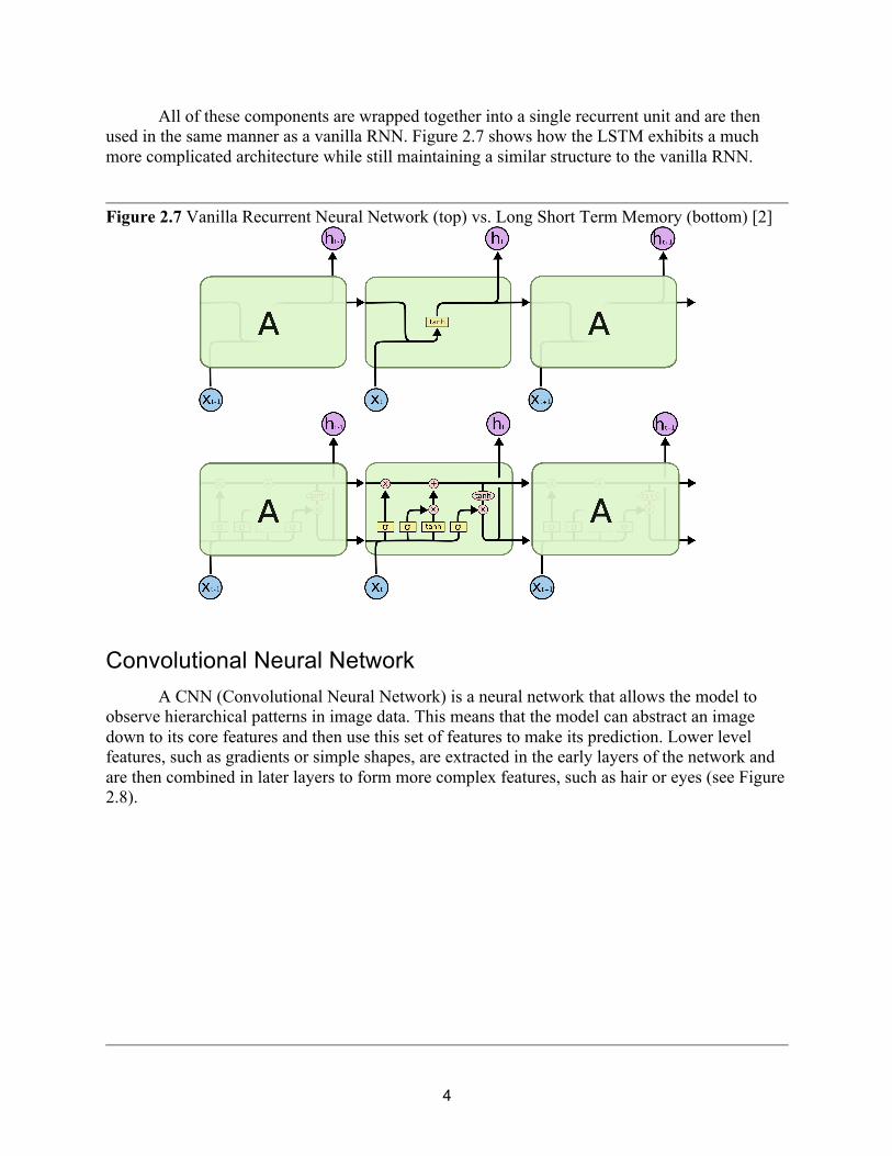
All of these components are wrapped together into a single recurrent unit and are then used in the same manner as a vanilla RNN. Figure 2.7 shows how the LSTM exhibits a much more complicated architecture while still maintaining a similar structure to the vanilla RNN.

Figure 2.7 Vanilla Recurrent Neural Network (top) vs. Long Short Term Memory (bottom) [2]

Convolutional Neural Network A CNN (Convolutional Neural Network) is a neural network that allows the model to observe hierarchical patterns in image data. This means that the model can abstract an image down to its core features and then use this set of features to make its prediction. Lower level features, such as gradients or simple shapes, are extracted in the early layers of the network and are then combined in later layers to form more complex features, such as hair or eyes (see Figure 2.8).

5

Figure 2.8 CNN Features Extracted in Early Layers (left) vs. Later Layers (right) [17]

One of the biggest advantages of using a CNN is that it reduces the number of learned parameters by using a group of shared weights, called a kernel. This allows for deeper models and thus more layers of abstraction to build upon. These kernels act as a sliding window that reduce the size of the next input by extracting the important features, ultimately leading to an embedding which captures the high level information contained in the original image. This embedding can then be passed into a feedforward neural network to perform any final classification/predictions.

Figure 2.9 Feature Map (pink) Derived from a Kernel’s (yellow) Convolution [16]

Normalization Data needs to be normalized prior to being fed into most machine learning models to

speed up training. If the input vectors are not all on the same scale, the model will struggle to find weights that can accommodate for the high variance in the data. The goal of normalization is to change the values of the input data to be commensurate without distorting the relative differences between the data points. The standard way of doing this is to subtract the sample

6

mean from the data and then divide the result by the sample standard deviation. This ensures that all of the training data follows a similar distribution and is weighted roughly the same by the model, leading to significantly faster convergence rates.

Most deep learning models are comprised of many layers, with each previous layer being the input to the following layer. Normalizing the activations in between layers can have a similar effect as normalizing the initial input data. When normalization is performed in between the layers of a deep learning model, it is called batch normalization. Batch normalization was introduced by S. Ioffe and C. Szegedy to speed up training by reducing covariate shift, and accomplished this by normalizing in the same manner as described above (data - mean / standard deviation) with the addition of two parameters that the model can tune. Gamma (𝛾) is used to control how much the activations should be scaled prior to being fed to the next layer and Beta (𝛽) is used to control how much the activations should be shifted.

Figure 2.10: Batch Normalization Equation

These parameters allow the model to learn how much and when normalization should be

performed in-between layers to maximize performance on the training set. In addition to speeding up convergence, batch normalization has also been shown to act as a form of regularization, further improving model performance.

Figure 2.11 Data Before and After Normalization [15]

7

Dropout Dropout is a form of regularization used to ensure a model does not depend too heavily on any given activation, ultimately increasing the robustness of the model’s weights [3]. Dropout accomplishes this by randomly zeroing out weights during training, forcing the model to rely on all of the weights (features) instead of just a handful. This ends up slowing down the convergence of the model, leading to roughly twice the number of training iterations (epochs) to converge, but will result in a model that generalizes across unseen data significantly better.

Figure 2.12 Neural Network Connections with Dropout [9]

Skip Connections Using skip connections in a deep learning model is a powerful method for getting your model to train faster while also trying out complex new architectures. A skip connection in a neural network is an alternate path the model can pass data forward through, providing a way to skip layers within the model (see Figure 2.14). One motivation for skipping over layers is that it provides a way for the model to reuse activations from a previous layer which helps to avoid the vanishing gradients problem, leading to faster convergence. The other main reason for using skip connections is to avoid using model layers that hinder the performance of the model. Just as with other layers, the skip connection becomes an internal function that maps the previous layer’s output to the input for the next layer. It is quite simple for a skip connection to learn the identify function, which would allow the model to essentially ignore all the layers the skip connection passes (see Figure 2.13).

8

Figure 2.13 Skip Connection Identity Function

This is quite nice when you would like to experiment with adding new layers to an existing model and want to ensure the model can perform no worse than it did without the addition. The use of skip connections allows the model to learn not only the weights for each layer, but also what layers should be used.

Figure 2.14 Neural Network with Skip Connections [18]

Sentinel-2 Satellite The Sentinel-2 satellite is a satellite that was launched by the European Space Agency as part of the Copernicus Program. It covers the earth roughly every 5 days and has a resolution of 10 meters. Due to its high resolution and consistent coverage, this satellite is a popular choice for remote sensing, especially for the monitoring of vegetation. The Sentinel-2 satellite produces imagery containing 13 spectral bands representing TOA (Top of the Atmosphere) reflectance, and 3 quality assurance bands, such as a binary cloud mask. Using the dataset described later in this paper, our tests have shown that the cloud mask included with the satellite only captures roughly 9% of all clouds present in an image, showing the need for an improved cloud mask.

9

Figure 2.15 Calculating TOA reflectance via Satellite [10]

Related Prior Work Cloud detection and classification has been studied for many years and the research has produced many approaches with differing tradeoffs. One of the first successful projects was the FMask algorithm created by Woodcock et al. that used deterministic thresholds to classify cloud pixels [12]. It combines the red, blue, green, near infrared, and short-wave infrared bands of the satellite and tests each pixel against an array of thresholds. These thresholds were chosen by the researchers based off of properties of clouds and how they alter light on different wavelengths. A later research project done by Hollstein et al. took a similar approach as the FMask paper, but rather than choosing the thresholds themselves, they used a decision tree to learn the thresholds [13]. Both of these deterministic approaches work well if a rough idea of cloud presence is needed, but their weaknesses make them unsuitable for most industry applications. Their first flaw is that clouds at extreme heights or depths alter the values observed by the infrared wavelengths and cause obvious clouds to remain unmasked. Their second flaw is that because these algorithms run on individual pixels, cloud masks will often appear scattered as no adjacent pixels are referenced during classification. With the rise of deep learning, researchers have begun exploring new methods for building cloud masks. In fact, this has been a strong basis for a new startup Sentinel Hub, which is heavily focused on cloud detection in the Sentinel satellites [11]. They use a dense neural network on each pixel to create a probability that the pixel contains clouds. While the neural network model showed an improvement over the decision tree model, it continued to suffer from the issue with the cloud mask appearing scattered as the model was still run on each individual pixel. We previously performed experiments that showed that time-series information alone can be quite helpful when detecting clouds in satellite images. The experiments involved using

10

various curve fitting methods, such as cubic spline, on a single pixel’s values over time and classifying any values that fell too far from the curve. This process was quite robust and would classify nearly every instance of clouds in an image but the simplicity of the curve fitting allowed for false positives to occur during normal deviations (such as when a field is harvested and the color for that area dramatically shifts).

A New LSTM Approach The current industry standard cloud mask uses a fully connected neural network to classify a satellite image pixel by pixel. This approach works quite well for detecting opaque and cirrus clouds, but suffers to separate the clear pixels from the pixels covered by a cloud’s shadow. Our approach to this problem leverages the existing model architecture to retain the high performance on the cloud detection, while adding an LSTM network to help assist the model detect cloud shadow. The LSTM will take a sequence of the previous pixel values over the last 5 days to create its embedding. The rationale behind this approach is that the model will be able to see when the pixel rapidly darkens, leading to a ‘shadow’ classification. In addition to the LSTM network, a skip connection is added around the LSTM. This skip connection will allow the model to bypass the LSTM network should it end up hindering performance.

In the following sections, we will describe our LSTM approach, starting with the dataset we used for training. We will next look at the models and methods employed. Finally, we will discuss our results and point the way to follow-on work.

Dataset

Data Collection and Split For training our LSTM, we will use a dataset comprised of 1 year of imagery (2018) of

randomly selected agricultural areas from around the world, totaling to 3549 labeled Sentinel-2 satellite images. The images were labeled down to the pixel level by an expert team of labelers, with each pixel being classified as either cloud free, opaque clouds, cirrus clouds, or cloud shadow. The labeled images were commissioned by and generously provided to our group by a team from Google[X] interested in solving this problem, as all the publically available datasets contain no more than 30-50 labeled images. The raw satellite images are publically available through the Google Earth Engine platform, but the labels are proprietary data and thus cannot be released.

There are 39 unique areas evenly represented by the dataset. 31 of these locations were randomly chosen for training and validations sets, while the remaining 8 were used as a test set for calculating the results for each model. The sets remained consistent for each model used during experimentation.

Each satellite image is roughly 750x1000 pixels, and so only a subset of pixels from each image was used during training. This subset was randomly chosen for each image, but it was ensured that each model still received the same pixels when the data format was changed from single to sequential.

11

Dataset Example

Model Architecture & Methods

Data Preprocessing The Sentinel-2 satellite bands contain values between 0-10,000, which differs from the normal 255 RGB scale that most images follow. Furthermore, because of how the TOA reflectance is calculated, the image values could not simply be divided by 10,000 to normalize the values. Instead, it was found that clipping the values to be between 0-2048, and then dividing the band values by 2048 provided the best results when validating using the red, green, and blue bands. To improve the rate of convergence, the clipped satellite images were preprocessed prior to being fed into the models. A random sample of 300 images was used to get the mean pixel value and standard deviation for each band. These band means and standard deviations were then used to normalize any training/testing sets by subtracting the means from the sets’ pixel values and then dividing the result by the standard deviations. Classically, when using machine learning to perform multiple classification problems, the training dataset will contain an equal number of labels for each class. However, there are not many labeled cloud images that are available for public use/research, and so the datasets used for cloud detection in other papers have used all available data they had. This means that their training sets were not evenly split and mostly likely were dominated by ‘clear’ labels. Even though the dataset used for this paper is large enough to drop examples and split the labels evenly, it was decided that sticking with the original distribution would allow for an easier comparison with other techniques. It should be noted that the results presented in the results section are most likely reflecting this bias caused from training imbalance.

Fully Connected Model (Baseline) The Sentinel Hub team showed that using a fully connected (dense) neural network

improved accuracy when compared to the classic FMask algorithm [11]. Their model is known

12

for its robustness and has been the go-to cloud mask for many industry remote sensing tasks. We recreated their model in Keras and used it as a baseline to compare the results of the LSTM model. The model architecture used for comparison can be seen in Figure 5.1. The model takes the band values for a single pixel as input. The band values are then fed through a simple feed forward network with relu activations, with the final layer performing a softmax activation to get the final classification prediction. Dropout layers are used periodically in-between the fully connected layers to help combat overfitting. The model’s hyperparameters were tuned using grid search, and the model’s weights were optimized using the Adam optimizer.

Figure 5.1 Fully Connected Cloud Detection Model Architecture

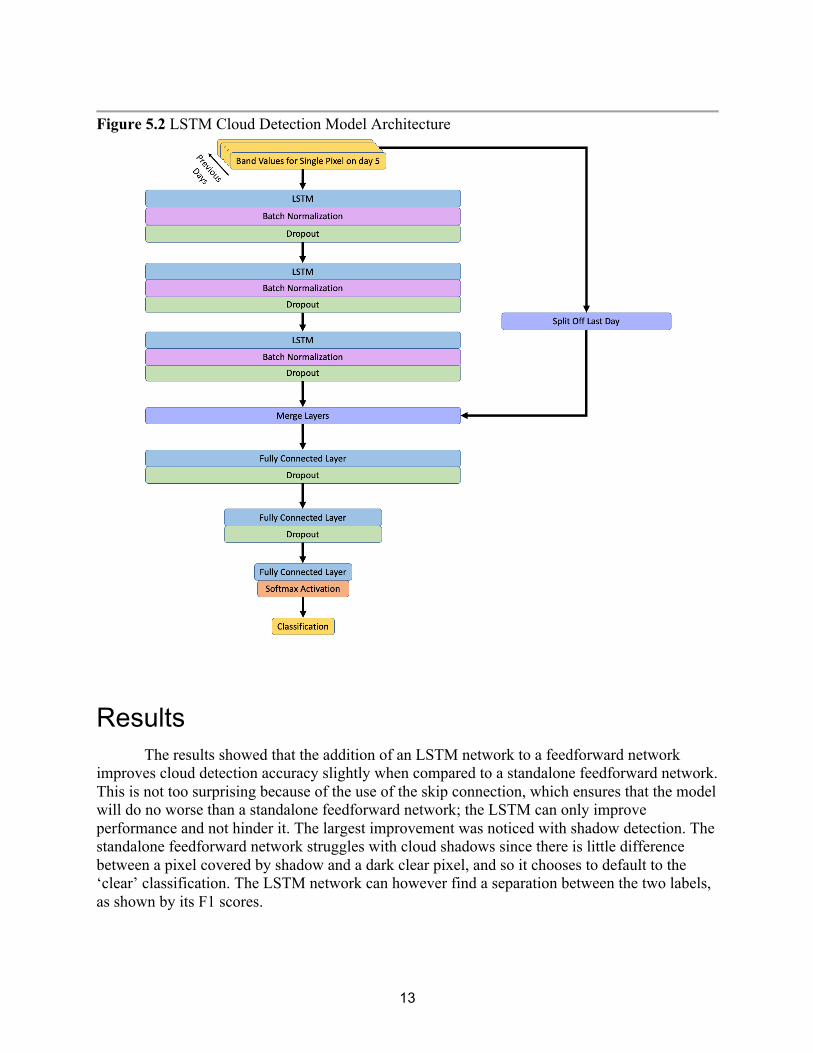
Fully Connected Model with LSTM Embedding The same fully connected network described above was used in the LSTM model for consistency. The only difference in this model is the inclusion of the LSTM layers at the top of the network. With this addition, the fully connected network receives the LSTM embedding and the original band values as input, rather than just the raw band values for the pixel. The LSTM embedding is considered a black box as the exact values are uninterpretable, but one could imagine that this embedding contains how each band’s current values differed from the values observed in previous days. The model takes the band values for a single pixel for the current day and the previous 5 days as input. The sequential band values are passed through the LSTM layers to extract the relationship between them before being merged with the original values for the current day. This skip connection ensures that the LSTM layers cannot hurt the model, but can only add more information via the LSTM embedding, should the network choose to use it. Just as with the baseline network, the model’s hyperparameters were tuned using grid search, and the model’s weights were optimized using the Adam optimizer.

13

Figure 5.2 LSTM Cloud Detection Model Architecture

Results The results showed that the addition of an LSTM network to a feedforward network improves cloud detection accuracy slightly when compared to a standalone feedforward network. This is not too surprising because of the use of the skip connection, which ensures that the model will do no worse than a standalone feedforward network; the LSTM can only improve performance and not hinder it. The largest improvement was noticed with shadow detection. The standalone feedforward network struggles with cloud shadows since there is little difference between a pixel covered by shadow and a dark clear pixel, and so it chooses to default to the ‘clear’ classification. The LSTM network can however find a separation between the two labels, as shown by its F1 scores.

14

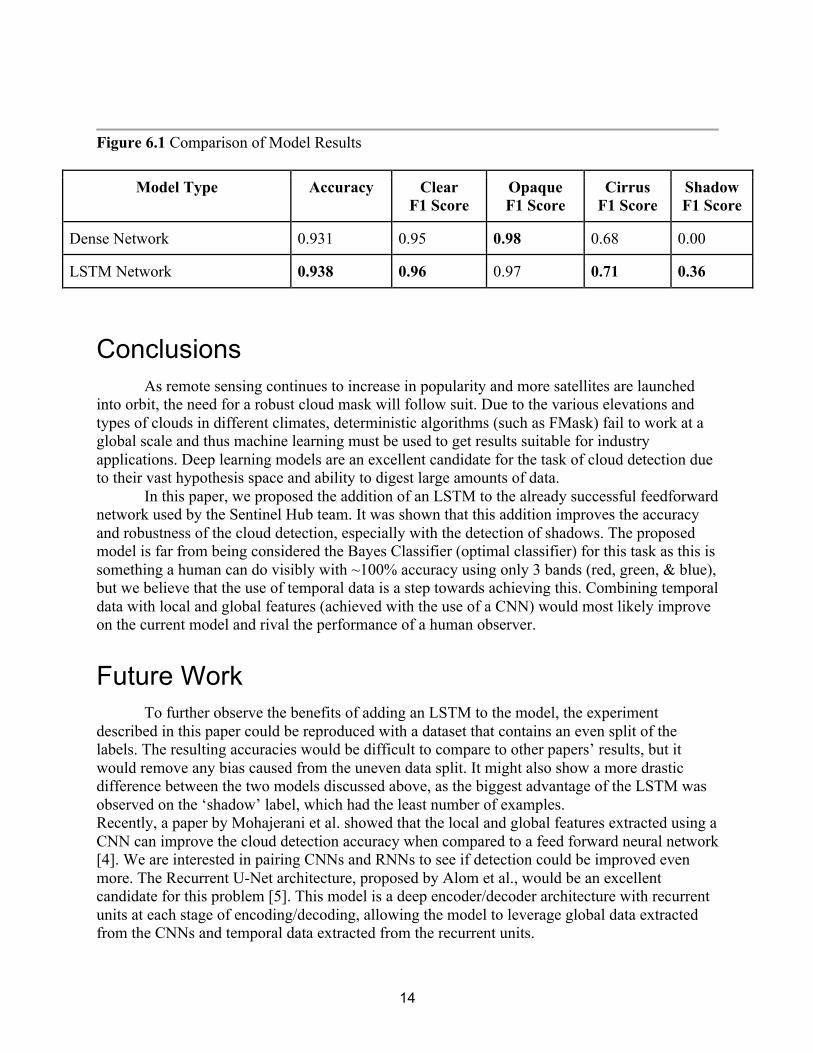
Figure 6.1 Comparison of Model Results

Model Type Accuracy Clear F1 Score

Opaque F1 Score

Cirrus F1 Score

Shadow F1 Score

Dense Network 0.931 0.95 0.98 0.68 0.00

LSTM Network 0.938 0.96 0.97 0.71 0.36

Conclusions As remote sensing continues to increase in popularity and more satellites are launched into orbit, the need for a robust cloud mask will follow suit. Due to the various elevations and types of clouds in different climates, deterministic algorithms (such as FMask) fail to work at a global scale and thus machine learning must be used to get results suitable for industry applications. Deep learning models are an excellent candidate for the task of cloud detection due to their vast hypothesis space and ability to digest large amounts of data. In this paper, we proposed the addition of an LSTM to the already successful feedforward network used by the Sentinel Hub team. It was shown that this addition improves the accuracy and robustness of the cloud detection, especially with the detection of shadows. The proposed model is far from being considered the Bayes Classifier (optimal classifier) for this task as this is something a human can do visibly with ~100% accuracy using only 3 bands (red, green, & blue), but we believe that the use of temporal data is a step towards achieving this. Combining temporal data with local and global features (achieved with the use of a CNN) would most likely improve on the current model and rival the performance of a human observer.

Future Work To further observe the benefits of adding an LSTM to the model, the experiment

described in this paper could be reproduced with a dataset that contains an even split of the labels. The resulting accuracies would be difficult to compare to other papers’ results, but it would remove any bias caused from the uneven data split. It might also show a more drastic difference between the two models discussed above, as the biggest advantage of the LSTM was observed on the ‘shadow’ label, which had the least number of examples. Recently, a paper by Mohajerani et al. showed that the local and global features extracted using a CNN can improve the cloud detection accuracy when compared to a feed forward neural network [4]. We are interested in pairing CNNs and RNNs to see if detection could be improved even more. The Recurrent U-Net architecture, proposed by Alom et al., would be an excellent candidate for this problem [5]. This model is a deep encoder/decoder architecture with recurrent units at each stage of encoding/decoding, allowing the model to leverage global data extracted from the CNNs and temporal data extracted from the recurrent units.

15

Figure 8.1 Recurrent U-Net Architecture [5]

16

Bibliography [1] S. Hochreiter and J. Schmidhuber, Long short-term memory, Neural computation, vol. 9,

no. 8, pp. 17351780, 1997.

[2] Olah, Christopher. Understanding LSTM Networks. http://colah.github.io/posts/2015-08-Understanding-LSTMs/, 2015.

[3] G. E. Hinton, N. Srivastava, A. Krizhevsky, I. Sutskever, and R. R. Salakhutdinov. Improving neural networks by preventing coadaptation of feature detectors. arXiv:1207.0580, 2012.

[4] Sorour Mohajerani: Cloud-Net: An end-to-end Cloud Detection Algorithm for Landsat 8

Imagery. arXiv:1901.10077, 2019.

[5] M. Z. Alom, M. Hasan, C. Yakopcic, T. M. Taha, and V. K. Asari, “Recurrent Residual Convolutional Neural Network based on U-Net (R2U-Net) for Medical Image Segmentation,” arXiv preprint arXiv:1802.06955, 2018.

[6] Planet. Planet Closes $168M Series D Financing. https://www.planet.com/pulse/planet-closes-168m-series-d-financing/, 2019.

[7] Wikipedia. Feedforward Neural Network. https://en.wikipedia.org/wiki/Feedforward_neural_network, 2006.

[8] Wikipedia. Recurrent Neural Network. https://en.wikipedia.org/wiki/Recurrent_neural_network, 2017.

[9] Srivastava, Nitish, et al. Dropout: a simple way to prevent neural networks from overfitting, JMLR, 2014.

[10] United Nations Office for Outer Space Affairs. Top of the Atmosphere. http://www.un-spider.org/node/10958, 2014. [11] Anze Zupanc. Improving Cloud Detection with Machine Learning.

https://medium.com/sentinel-hub/improving-cloud-detection-with-machine-learning-c09dc5d7cf13, 2017.

[12] Zhu, Z. & Woodcock, C. E. Object-based cloud and cloud shadow detection in Landsat imagery. Remote Sens. Environ. 118, 83–94. 2012. [13] Hollstein, A.; Segl, K.; Guanter, L.; Brell, M.; Enesco, M. Ready-to-Use Methods for the Detection of Clouds, Cirrus, Snow, Shadow, Water and Clear Sky Pixels in Sentinel-2 MSI Images. Remote Sens. 8, 666. 2016.

[14] Hochreiter, Sepp & Schmidhuber, Jürgen. Long Short-term Memory. Neural

17

computation. 9. 1735-80. 1997. [15] Joseph Santarcangelo. Data Normalization and Standardization. https://www.mathworks.com/matlabcentral/fileexchange/48677-data-normalization-and-

standardization. 2015. [16] Denny Britz. Understanding Convolutional Neural Networks for NLP. http://www.wildml.com/2015/11/understanding-convolutional-neural-networks-for-nlp. 2015. [17] Evan Shelhamer. Deep Learning for Computer Vision with Caffe and cuDNN. https://devblogs.nvidia.com/deep-learning-computer-vision-caffe-cudnn. 2014. [18] Xavier Giró-i-Nieto. Deep Learning for Speech and Language. https://www.slideshare.net/xavigiro/advanced-deep-architectures-d2l6-deep-learning- for-speech-and-language-upc-2017. 2017.