Deep Reinforcement Learning for Simulated Autonomous Vehicle Control

April Yu, Raphael Palefsky-Smith, Rishi BediStanford University

{aprilyu, rpalefsk, rbedi} @ stanford.edu

Abstract

We investigate the use of Deep Q-Learning to control asimulated car via reinforcement learning. We start by im-plementing the approach of [5] ourselves, and then exper-imenting with various possible alterations to improve per-formance on our selected task. In particular, we experimentwith various reward functions to induce specific driving be-havior, double Q-learning, gradient update rules, and otherhyperparameters.

We find we are successfully able to train an agent to con-trol the simulated car in JavaScript Racer [3] in some re-spects. Our agent successfully learned the turning oper-ation, progressively gaining the ability to navigate largersections of the simulated raceway without crashing. Inobstacle avoidance, however, our agent faced challengeswhich we suspect are due to insufficient training time.

1. IntroductionCurrently, self-driving cars employ a great deal of expen-

sive and complex hardware to achieve autonomous motion.We wanted to explore the possibility of utilizing a cheapeveryday camera to enable a car to drive itself. Our mainquestion was whether we could learn simple driving poli-cies from video alone. Current autonomous driving imple-mentations have shied away from the computer vision tech-niques because of a lack of robustness. The inaccuracieswith vision-based autonomous driving systems lie mostlyin the difficulty of compressing the input image into a com-pact but representative feature vector. There are currentlytwo approaches to this problem: ”mediated perception ap-proaches” parse an entire scene (input image) to make adriving decision and ”behavior reflex approaches” utilize aregressor to directly map an input image to a driving ac-tion. [2]. Neither of these approaches has been resound-ingly successful. Because of this, we ultimately turned toautonomous driving through end-to-end Deep Q-Learning.

However, the ability to test these techniques and the var-ious related experiments with an actual car on real-videodata was out of the question, given the reinforcement-

learning nature of the paradigm. Instead, we turned toJavaScript Racer (a very simple browser-based JavaScriptracing game), which allowed us to easily experiment withvarious modifications to Deep Q-Learning, hyperparame-ters and reward functions.

2. Related WorkQ-Learning (further explained in the Methods section)

was introduced by Chris Watkins in his Ph.D. thesis. [10]Inspired by animal psychology, Watkins sought to developa method which allows for the efficient learning of an opti-mal strategy to accomplish arbitrary tasks which can be for-mulated as Markov Decision Processes. While supervisedlearning can often learn action policies as well, ”sequentialprediction” problems are often better served by reinforce-ment learning approaches, where the model has some levelof interaction during the learning process. [7]

In 2005, Riedmiller introduced the idea of using neu-ral network approximators for the Q function in Q-learning.[6] Mnih et al. introduced the idea of image-based DeepQ-Learning in 2015, when the group at DeepMind success-fully used a convolutional neural network (DQN) to learna Q function which successfully plays various Atari 2600games at or significantly above professional human playerability. The only inputs to their DQN algorithm were im-ages of the game state and reward function values. [5] Mostimpressively, this paper utilizes a single learning paradigmto successfully learn a wide variety of games - the gen-eralizability of the approach (while obviously not a singleset of learned parameters) is powerful, and is what inspiredus to attempt to apply their model to learning a policy forJavaScript Racer.

Since that work, DeepMind and others have publishednumerous extensions to the DQN paradigm. We will sum-marize some of those extensions here, some of which welater choose to implement variations of to seek to improveour agent’s performance.

DQN learning approaches have been successfully lever-aged for continuous control in addition to discrete controltasks. While we ultimately modeled our simulated car driv-ing problem as a discrete learning task, the task of simulated

1

car control has been well-studied as a continuous controlproblem as well. [4]

Some popular DQN modifications we explore includeprioritized experience replay and double DQN, the detailsof which are explained in Methods [9].

State-of-the-art autonomous vehicle control algorithmsare largely orthogonal to DQN approaches, and since thevery simplified game we ended up playing bears few actualsimilarities to real-world autonomous driving, the substan-tial body of literature that exists in that field was not espe-cially relevant to our work here. DQN-based approaches tosimple video games were much more in the vein of the workdone in this paper, and thus form the core body of work onwhich our experiments are based.

3. MethodsWe began our project by re-implementing the Deep Q-

Learning algorithm ourselves [5] as presented by the teamat Google DeepMind, using TensorFlow [1]. Our imple-mentation can be found on GitHub: https://github.com/RaphiePS/cs231n-project. This algorithmextends the general Q-Learning reinforcement learning al-gorithm to adapt to an infinitely larger state space. In vanillaQ-Learning, the algorithm learns an action-value functionthat ultimately gives the expected utility of taking a givenaction in a given state. The implementation of vanilla Q-Learning keeps track of these (state - action - new state)transitions and the respective reward in a table and updatesthese values in the table as it continues to train. With eachtraining point, the Q function estimates the expected rewardfor taking a particular action from a particular state to ar-rive at a new state and picks the action that maximizes thisreward. With the knowledge of the actual observed rewardr and the next state s’, we are able to calculate the relativeerror for that particular state-action-new state transition (us-ing γ as a discount for future rewards):

error = (r + γmaxa′Q(s′, a′))−Q(S, a) (1)

where the minuend is the actual reward and the subtrahendis the reward predicted by our action-value function. Withthis calculated error, we are able to update the transition ta-ble by adding it to the existing Q value for the particularstate-action-new state. These incremental updates gradu-ally transform the Q-function from a table of random noiseto an effective game-playing agent. However, when the in-put to the algorithm is an image, the state space becomesprohibitively large and this transition matrix implementa-tion is no longer practical. Instead, a convolutional neuralnetwork (CNN) is used as the Q-function approximator andthe error is backpropagated to update the network with eachminibatch of training examples, such that the parameters ofthe CNN learn a good non-linear approximation of the Q-function even for states it has not explicitly seen before.

We implemented the same CNN architecture (Figure 1)as proposed by Mnih et al [5], with 3 convolutional layersand 2 fully connected layers.

Figure 1. Convolutional Neural Network Architecture

The naive implementation of Deep Q-Learning is thesimple swapping of a table-based Q function for a CNN.However, this setup is unstable and can lead to a sort of”overfitting,” where updating the neural network from themost recent experiences hurts the agent’s performance inthe immediate future. Thus, Mnih et al [5] propose twomodifications, both of which are designed to prevent the al-gorithm from focusing on the most recent frames and helpit smooth over irregularities. These can be thought of as asort of ”temporal regularization,” and they help the agentconverge much faster.

The first of these methods is called experience replay,and it draws inspiration from learning mechanisms in ac-tual neuroscience. The key idea is to update the net-work using all of its past experiences, not just recentframes. To perform experience replay, we store experienceset = (st, at, rt, st+1) at each time-step t into the expe-rience replay buffer Bt = {e1, ..., et}. During training,we apply Q-learning updates on minibatches of experience(s, a, r, s′) ∼ U(B). Note that these minibatches are drawnuniformly from the buffer. Mnih et al [5] acknowledgesthat this is a shortcoming - every frame is equally likelyto be sampled to update the network, yet it is obvious thatsome frames (e.g. entering a turn) are far more ”influen-tial” than others (say, driving down a straightaway). Therehas since been work aimed at more carefully sampling thereplay buffer, which is called prioritized experience replay.

The second ”regularization” technique applied by Mnihet al [5] is the use of not one, but two Convolutional NeuralNetworks to learn the Q function. In addition to the usualQ-network, they propose a second ”target” Q-network, des-ignated Q. This net is used solely to generate the targetvalues for the Q update - the regular Q-network is still usedto choose actions at each step. Thus, the error equation be-comes

error = (r + γmaxa′Q(s′, a′))−Q(s, a) (2)

2

While error is still backpropagated toQ, Q is never updatedvia backpropagation. Rather, every C frames (10,000 inour experiments), the parameters from Q are simply copiedover to Q. This temporal delay similarly prevents temporal”overfitting”.

Upon feedback we received at the Poster Session, we im-plemented the Double Q-Learning variant proposed by vanHasselt et al. [9] Double DQN is meant to alleviate theproblem of DQNs overestimating the value of a given ac-tion in some circumstances. Double DQN attempts to cor-rect for this by separating the selection and evaluation ofthe max function employed in the calculation of yj . Moreprecisely, Double DQN replaces the original target yj eval-uation function (in the non-trivial case where step j is non-terminal, otherwise yj = rj in both DQN and Double DQNalgorithms), which is

yj = rj + γmaxa′Q(φj+1, a′; θ−) (3)

with the following:

yj = rj + γQ(φj+1, arg maxa

Q(φj+1, a; θ), θ−) (4)

Also upon feedback we received, we replaced our un-clipped loss function with a simplified variant of Huber loss,instead of the original unclipped `2 loss function, with thegoal of improving the DQN’s stability.

loss = min(|∆Y |, |∆Y |2) (5)

As mentioned previously, the original DQN implemen-tation in [5] sampled uniformly from transition memory.The authors noted this as a potential area for improvement,which Schaul et al. attempted to correct. [8] This alter-ation extends the experience replay model by not simplyuniformly sampling transitions from memory, but instead,weighting individual transitions in memory with their ”TD-error”, an attempt to quantify the ”unexpectedness” of agiven transition, with the ultimate goal of allowing the DQNto replay ”important” transitions more frequently and there-fore learn more efficiently. The formula for TD-error (alsousing the Double Q-learning equation) is given as follows -essentially, it computes the difference between yj as com-puted by the Double DQN update and the Q value as com-puted by the other (non-target) network.

δj = rj+γQ(φj+1, arg maxa

Q(φj+1, a; θ); θ−)−Q(φj , a; θ)

(6)We implemented the binary-heap rank-based prioritiza-

tion approach described in appendix B2 of [8], where eachtransition is inserted into a binary heap. This heap is thenused as an approximation for a sorted array, and the array

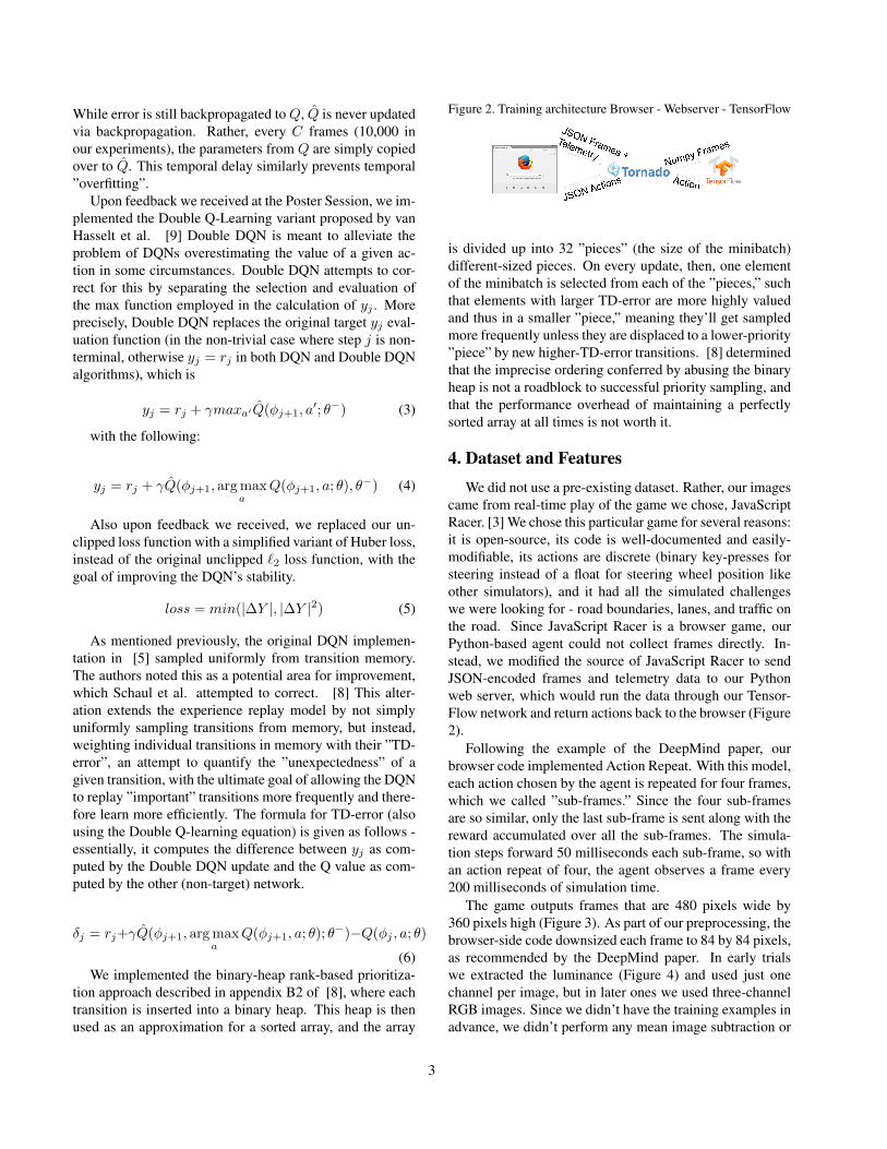
Figure 2. Training architecture Browser - Webserver - TensorFlow

is divided up into 32 ”pieces” (the size of the minibatch)different-sized pieces. On every update, then, one elementof the minibatch is selected from each of the ”pieces,” suchthat elements with larger TD-error are more highly valuedand thus in a smaller ”piece,” meaning they’ll get sampledmore frequently unless they are displaced to a lower-priority”piece” by new higher-TD-error transitions. [8] determinedthat the imprecise ordering conferred by abusing the binaryheap is not a roadblock to successful priority sampling, andthat the performance overhead of maintaining a perfectlysorted array at all times is not worth it.

4. Dataset and Features

We did not use a pre-existing dataset. Rather, our imagescame from real-time play of the game we chose, JavaScriptRacer. [3] We chose this particular game for several reasons:it is open-source, its code is well-documented and easily-modifiable, its actions are discrete (binary key-presses forsteering instead of a float for steering wheel position likeother simulators), and it had all the simulated challengeswe were looking for - road boundaries, lanes, and traffic onthe road. Since JavaScript Racer is a browser game, ourPython-based agent could not collect frames directly. In-stead, we modified the source of JavaScript Racer to sendJSON-encoded frames and telemetry data to our Pythonweb server, which would run the data through our Tensor-Flow network and return actions back to the browser (Figure2).

Following the example of the DeepMind paper, ourbrowser code implemented Action Repeat. With this model,each action chosen by the agent is repeated for four frames,which we called ”sub-frames.” Since the four sub-framesare so similar, only the last sub-frame is sent along with thereward accumulated over all the sub-frames. The simula-tion steps forward 50 milliseconds each sub-frame, so withan action repeat of four, the agent observes a frame every200 milliseconds of simulation time.

The game outputs frames that are 480 pixels wide by360 pixels high (Figure 3). As part of our preprocessing, thebrowser-side code downsized each frame to 84 by 84 pixels,as recommended by the DeepMind paper. In early trialswe extracted the luminance (Figure 4) and used just onechannel per image, but in later ones we used three-channelRGB images. Since we didn’t have the training examples inadvance, we didn’t perform any mean image subtraction or

3

similar normalization.

Figure 3. Full-color, full-sized frame.

Figure 4. After resizing and grayscaling.

In addition to raw frames, the browser also sends overtelemetry data, namely the car’s speed, its position on theroad, and whether a collision had occurred. The agent neverdirectly uses this data as input - it learned to make decisionsbased solely on the pixels in each frame. But JavaScriptRacer doesn’t have a game score, so this telemetry data wasused as input for our reward function, as described in theExperiments section below.

Telemetry Data Field Example ValueSpeed 35Max Speed Attainable 120X Position -0.2Collision Occurred FalseProgress around track 23%

After a forward pass through the Q-network, our algorithmreturned an action to send to the browser. This action con-sisted of four booleans, whether each key - left, right, faster,slower - would be pressed or not. Once we removed ille-gal actions (for instance, pressing left and right at the sametime), we were left with 9 discrete actions, as visualizedin Figure 5. After experimentation, we removed many ofthese actions, leaving us with only three: faster, faster-plus-left, and faster-plus-right. As expected, this led to a muchhigher average speed, as the car was unable to decelerate.

Figure 5. Full action space

As to the size of our dataset, our experiments utilizedbetween 200,000 and 600,000 frames. Since the game playsthe first 50,000 frames completely randomly and uses theseframes as fodder for the experience replay buffer, we wereable to reuse these frames across trials. Otherwise, eachtrial generated novel frames for its own use.

5. ExperimentsOur initial set of experiments used grayscale images

with an agent history length of 4 (i.e., four consecutiveframes fed as input to the DQN). Upon discovering a not-particularly-clear saliency map and less-than-satisfactoryperformance characterized by intermittent stopping of theagent along the racetrack, we suspected our network lackedthe ability to consistently differentiate important features onthe road. To help ameliorate this, we switched to start us-ing three-channel RGB images. To compensate for the in-creased computational cost of this larger input (most sig-nificantly, network traffic time), we reduced agent historylength to 1, so only one frame at a time was being evaluatedby the DQN. This was also at Andrej’s suggestion, who sug-gested debugging our implementation would be easier withthe net viewing single frames at a time.

We utilized multiple evaluation metrics to qualitativelyand quantitatively assess the relative success of a given ex-periment. One consistent challenge was striking a balancebetween confirming experiment reproducibility and tryingnew experiments, given limited time and computational re-sources. Some of our experiments may have resulted in out-lying results that may have been overturned given enoughrepeats. For the most part, however, we erred on the side ofmore, diverse experiments instead of confirming initial re-sults. In this sense, some of our ”quantitative” results havea more anecdotal flavor. On a related note, we chose torun a greater number of shorter-term experiments instead oftraining a single model for a very extended duration. Mostof our experiments terminated after 200,000 frames, withsome continuing to run until 600,000 frames. For context,Mnih et al. trained on 50 million frames for each Atarigame.

For quantitative evaluation of our agent’s performance,

4

we analyzed the average Q-value for a minibatch, the Huberloss associated with each gradient update, and the rollingaverage reward over some number of frames (say, 1000).These continuous metrics, while helpful for debugging andselecting hyperparameters, are often less enlightening thana simple video of the agent controlling the car, the mostsalient qualitative summary of our best model’s driving per-formance. While the increase in average reward may ap-pear relatively smooth, that belies the discrete jump learningwhich often happens (as, for example, the car learns how toround a turn it previously consistently crashed on).

We validate the generalizability of our learned model bytaking some fixed number of random actions before turningthe policy over to the model. This means that the world theDQN agent sees is stochastic and the frames are unlikelyto be identical to those it saw during training. In almostall cases, the agent is able to recover from whatever state itfinds itself in and complete the number of turns it was ableto when started deterministically.

We had greater success using a track with no cars on it(only turns and fixed obstacles), than a car with cars on it.While the agent learned to navigate turns successfully inboth, it exhibited only very sporadic ability to avoid cars,and those successes may have been the result of chancerather than true obstacle avoidance. Given the model’s abil-ity to learn turning successfully, we ascribe this inability toinsufficient training time.

We also had much quicker success by limiting the al-lowable actions. By eliminating slowing-down (i.e., onlyallowing forward, forward+right, forward+left), the agentwas much more quickly able to learn a sensible policy, asthe initial random exploration of the action space containedno frames where the car simply wasn’t moving. When thecar was allowed to choose to slow down / not move at all,it was still able to make turns, but after an equivalent num-ber of training frames (300k), had mastered only one turnwhile its action-limited counterpart was consistently round-ing four or five.

Initial bugs in our DQN implementation led us to exper-iment with alternative gradient update rules as a possiblesolution. We tried Adagrad, RMSProp, and Adam, to findthat our original choice (the same as in the Mnih et al. Deep-Mind paper) of RMSProp with momentum = 0.95 workedbest.

We tested multiple reward functions intended to inducedifferent driving behavior. The variables we considered in-clude: staying in a single driving lane (INLANE), progressaround the track (PROG), speed (S) as a fraction of maxspeed, and going off-road (O) or colliding with other vehi-cles / stationary objects on the course (C). Formally, the twovery different reward functions we tested were as follows:

S =current speed

maximum attainable speed(7)

R1 =

−5 C or O−10 S = 0

min(10, 0.2 + 5S) otherwise(8)

R2 =

−1 C

−0.8 O

−1 S = 0

S INLANE0.8S not INLANE

(9)

At first glance, both reward functions would seem similar -they both penalize collisions and standing still, and rewardacceleration proportional to the car’s speed. However, wefound that the choice of reward function dramatically af-fected our learning performance. When we plotted the av-erage reward per episode vs the update iteration, we foundthat the reward function R2 performed significantly better,as seen in Figure 6 with R1 above R2. In fact, using R1 ouragent didn’t seem to learn anything at all.

Figure 6. Average episode reward, with R1 on top and R2 below.These experiments were conducted with all nine actions allowable(including no-ops and slowing down).

In addition to various reward functions, we tested differ-ent learning rates. Our first model which learned unambigu-ously and convincingly was an RMSProp implementation

5

with a reward function optimized for staying in the lane ona track with no other cars on it. Video of one sample run ofthis agent can be found here: https://www.youtube.com/watch?v=zly8kuaNvsk. We then used this as thebaseline against which to compare alternative models. Theperformance of various learning rates is visualized in Figure7. Upon selecting the reward function and gradient updaterule, we held these as fixed for the remainder of our experi-ments.

Figure 7. Reward function over varying learning rates.

It was immediately clear that a learning rate of 0.001 wastoo steep, but differentiating between the remaining learn-ing rates was less obvious, so we turned to a visualizationof the loss function, which made it clearer that .0001 wasthe preferred option. This choice was validated by viewingthe car driving - the LR=.0001 agent made it around moreturns with greater consistency than any of the other agents.Varying the learning rate was the next most significant de-terminant of qualitative success after reward functions andupdate rules (Figure 8).

Figure 8. Loss function over varying learning rates.

We examined the percentage of actions selected as a san-ity check of the policy the agent learned (Figure 9). Reas-suringly, the selection of left to right turns was almost iden-tical, and the car consistently accelerated.

Figure 9. Actions selected by best model so far

As another qualitative evaluation, we generated a t-SNEembedding of points in our final connected layer. Clearclustering is evident in both action coloring and Q-valuecoloring. Again inspired by [5], we visualized a samplingof some of the states in these distinct clusters. In Figure10A, yellow corresponds to move left, blue corresponds tomove right, and purple corresponds to move straight in thecurrent direction. The frames we visualized justify these la-bels: in the highlighted point which is blue, for example, thecar is clearly veering to the left side of the road and is bestfollowed by a move to the right to correct course. Similarrational labeling is observed in Figure 10B.

Figure 10. t-SNE embedding of 10,000 randomly selected pointsin final connected layer (a) - colored by action selected by agent inthat state, (b) - colored by predicted Q-value of state.

6

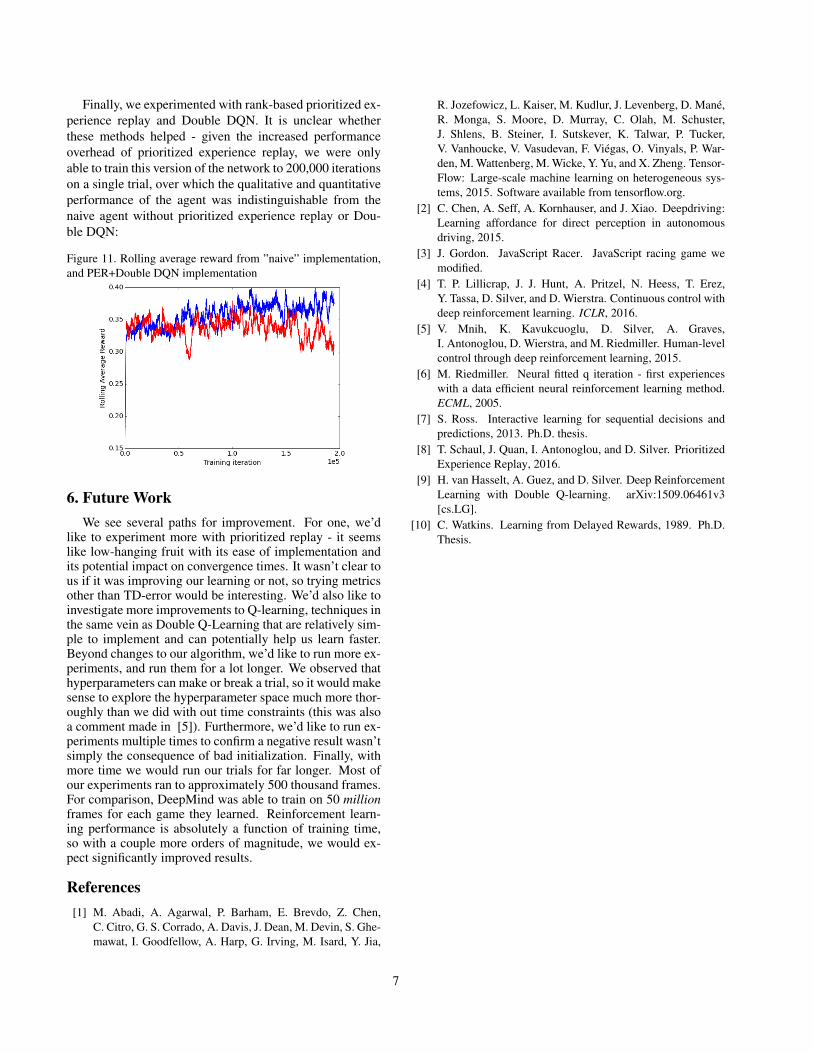
Finally, we experimented with rank-based prioritized ex-perience replay and Double DQN. It is unclear whetherthese methods helped - given the increased performanceoverhead of prioritized experience replay, we were onlyable to train this version of the network to 200,000 iterationson a single trial, over which the qualitative and quantitativeperformance of the agent was indistinguishable from thenaive agent without prioritized experience replay or Dou-ble DQN:

Figure 11. Rolling average reward from ”naive” implementation,and PER+Double DQN implementation

6. Future WorkWe see several paths for improvement. For one, we’d

like to experiment more with prioritized replay - it seemslike low-hanging fruit with its ease of implementation andits potential impact on convergence times. It wasn’t clear tous if it was improving our learning or not, so trying metricsother than TD-error would be interesting. We’d also like toinvestigate more improvements to Q-learning, techniques inthe same vein as Double Q-Learning that are relatively sim-ple to implement and can potentially help us learn faster.Beyond changes to our algorithm, we’d like to run more ex-periments, and run them for a lot longer. We observed thathyperparameters can make or break a trial, so it would makesense to explore the hyperparameter space much more thor-oughly than we did with out time constraints (this was alsoa comment made in [5]). Furthermore, we’d like to run ex-periments multiple times to confirm a negative result wasn’tsimply the consequence of bad initialization. Finally, withmore time we would run our trials for far longer. Most ofour experiments ran to approximately 500 thousand frames.For comparison, DeepMind was able to train on 50 millionframes for each game they learned. Reinforcement learn-ing performance is absolutely a function of training time,so with a couple more orders of magnitude, we would ex-pect significantly improved results.

References[1] M. Abadi, A. Agarwal, P. Barham, E. Brevdo, Z. Chen,

C. Citro, G. S. Corrado, A. Davis, J. Dean, M. Devin, S. Ghe-mawat, I. Goodfellow, A. Harp, G. Irving, M. Isard, Y. Jia,

R. Jozefowicz, L. Kaiser, M. Kudlur, J. Levenberg, D. Mane,R. Monga, S. Moore, D. Murray, C. Olah, M. Schuster,J. Shlens, B. Steiner, I. Sutskever, K. Talwar, P. Tucker,V. Vanhoucke, V. Vasudevan, F. Viegas, O. Vinyals, P. War-den, M. Wattenberg, M. Wicke, Y. Yu, and X. Zheng. Tensor-Flow: Large-scale machine learning on heterogeneous sys-tems, 2015. Software available from tensorflow.org.

[2] C. Chen, A. Seff, A. Kornhauser, and J. Xiao. Deepdriving:Learning affordance for direct perception in autonomousdriving, 2015.

[3] J. Gordon. JavaScript Racer. JavaScript racing game wemodified.

[4] T. P. Lillicrap, J. J. Hunt, A. Pritzel, N. Heess, T. Erez,Y. Tassa, D. Silver, and D. Wierstra. Continuous control withdeep reinforcement learning. ICLR, 2016.

[5] V. Mnih, K. Kavukcuoglu, D. Silver, A. Graves,I. Antonoglou, D. Wierstra, and M. Riedmiller. Human-levelcontrol through deep reinforcement learning, 2015.

[6] M. Riedmiller. Neural fitted q iteration - first experienceswith a data efficient neural reinforcement learning method.ECML, 2005.

[7] S. Ross. Interactive learning for sequential decisions andpredictions, 2013. Ph.D. thesis.

[8] T. Schaul, J. Quan, I. Antonoglou, and D. Silver. PrioritizedExperience Replay, 2016.

[9] H. van Hasselt, A. Guez, and D. Silver. Deep ReinforcementLearning with Double Q-learning. arXiv:1509.06461v3[cs.LG].

[10] C. Watkins. Learning from Delayed Rewards, 1989. Ph.D.Thesis.

7