Deep Network Flow for Multi-Object Tracking

Samuel Schulter Paul Vernaza Wongun Choi Manmohan ChandrakerNEC Laboratories America, Media Analytics Department

Cupertino, CA, USA{samuel,pvernaza,wongun,manu}@nec-labs.com

Abstract

Data association problems are an important componentof many computer vision applications, with multi-objecttracking being one of the most prominent examples. A typi-cal approach to data association involves finding a graphmatching or network flow that minimizes a sum of pair-wise association costs, which are often either hand-craftedor learned as linear functions of fixed features. In thiswork, we demonstrate that it is possible to learn featuresfor network-flow-based data association via backpropaga-tion, by expressing the optimum of a smoothed network flowproblem as a differentiable function of the pairwise associ-ation costs. We apply this approach to multi-object trackingwith a network flow formulation. Our experiments demon-strate that we are able to successfully learn all cost func-tions for the association problem in an end-to-end fashion,which outperform hand-crafted costs in all settings. The in-tegration and combination of various sources of inputs be-comes easy and the cost functions can be learned entirelyfrom data, alleviating tedious hand-designing of costs.

1. IntroductionMulti-object tracking (MOT) is the task of predicting

the trajectories of all object instances in a video sequence.MOT is challenging due to occlusions, fast moving objectsor moving camera platforms, but it is an essential module inmany applications like action recognition, surveillance orautonomous driving. The currently predominant approachto MOT is tracking-by-detection [3, 7, 10, 15, 26, 33, 41],where, in a first step, object detectors like [16, 43, 51] pro-vide potential locations of the objects of interest in the formof bounding boxes. Then, the task of multi-object trackingtranslates into a data association problem where the bound-ing boxes are assigned to trajectories that describe the pathof individual object instances over time.

Bipartite graph matching [25, 35] is often employed inon-line approaches to assign bounding boxes in the currentframe to existing trajectories [22, 37, 38, 52]. Off-line meth-

ods can be elegantly formulated in a network flow frame-work to solve the association problem including birth anddeath of trajectories [27, 29, 54]. Section 2 gives more ex-amples. All these association problems can be solved in alinear programming (LP) framework, where the constraintsare given by the problem. The interplay of all variables inthe LP, and consequently their costs, determines the successof the tracking approach. Hence, designing good cost func-tions is crucial. Although cost functions are hand-crafted inmost prior work, there exist approaches for learning costsfrom data. However, they either do not treat the problem asa whole and only optimize parts of the costs [27, 31, 52, 54]or are limited to linear cost functions [49, 50].

We propose a novel formulation that allows for learningarbitrary parameterized cost functions for all variables ofthe association problem in an end-to-end fashion, i.e., frominput data to the solution of the LP. By smoothing the LP,bi-level optimization [6, 13] enables learning of all the pa-rameters of the cost functions such as to minimize a lossthat is defined on the solution of the association problem,see Section 3.2. The main benefit of this formulation is itsflexibility, general applicability to many problems and theavoidance of tedious hand-crafting of cost functions. Ourapproach is not limited to log-linear models (c.f ., [49]) butcan take full advantage of any differentiable parameterizedfunction, e.g., neural networks, to predict costs. Indeed, ourformulation can be integrated into any deep learning frame-work as one particular layer that solves a linear programin the forward pass and back-propagates gradients w.r.t. thecosts through its solution (see Figure 2).

While our approach is general and can be used formany association problems, we explore its use for multi-object tracking with a network flow formulation (see Sec-tions 3.1 and 3.4). We empirically demonstrate on publicdata sets [17, 28, 32] that: (i) Our approach enables end-to-end learning of cost functions for the network flow problem.(ii) Integrating different types of input sources like bound-ing box information, temporal differences, appearance andmotion features becomes easy and all model parameters canbe learned jointly. (iii) The end-to-end learned cost func-

tions outperform hand-crafted functions without the need tohand-tune parameters. (iv) We achieve encouraging resultswith appearance features, which suggests potential benefitsfrom end-to-end integration of deep object detection andtracking, as enabled by our formulation.

2. Related WorkAssociation problems in MOT: Recent works on multi-object tracking (MOT) mostly follow the tracking-by-detection paradigm [3, 7, 10, 15, 26, 33, 41], where ob-jects are first detected in each frame and then associatedover time to form trajectories for each object instance. On-line methods like [8, 11, 15, 39, 41] associate detectionsof the incoming frame immediately to existing trajectoriesand are thus appropriate for real-time applications1. Tra-jectories are typically treated as state-space models likeKalman [21] or particle filters [18]. The association tobounding boxes in the current frame is often formulated asbipartite graph matching and solved via the Hungarian al-gorithm [25, 35]. While on-line methods only have accessto the past and current observations, off-line (or batch) ap-proaches [3, 9, 20, 1, 40, 54] also consider future frames oreven the whole sequence at once. Although not applicablefor real-time applications, the advantage of batch methodsis the temporal context allowing for more robust and non-greedy predictions. An elegant solution to assign trajecto-ries to detections is the network flow formulation [54] (seeSection 3.1 for details). Both of these association modelscan be formulated as linear program.

Cost functions: Independent of the type of associationmodel, a proper choice of the cost function is crucial forgood tracking performance. Many works rely on care-fully designed but hand-crafted functions. For instance,[29, 33, 41] only rely on detection confidences and spa-tial (i.e., bounding box differences) and temporal distances.Zhang et al. [54] and Zamir et al. [53] include appearanceinformation via color histograms. Other works explicitlylearn affinity metrics, which are then used in their trackingformulation. For instance, Li et al. [31] build upon a hi-erarchical association approach where increasingly longertracklets are combined into trajectories. Affinities betweentracklets are learned via a boosting formulation from vari-ous hand-crafted inputs including length of trajectories andcolor histograms. This approach is extended in [26] bylearning affinities on-line for each sequence. Similarly, Baeand Yoon [2] learn affinities on-line with a variant of lin-ear discriminant analysis. Song et al. [47] train appearancemodels on-line for individual trajectories when they are iso-lated, which can then be used to disambiguate from othertrajectories in difficult situations like occlusions or interac-tions. Leal-Taixe et al. [27] train a Siamese neural network

1In this context, real-time refers to a causal system.

to compare the appearance (raw RGB patches) of two detec-tions and combine this with spatial and temporal differencesin a boosting framework. These pair-wise costs are used in anetwork flow formulation similar to [29]. In contrast to ourapproach, none of these methods consider the actual infer-ence model during the learning phase but rely on surrogateloss functions for parts of the tracking costs.Integrating inference into learning: Similar to our ap-proach, there have been recent works that also include thefull inference model in the training phase. In particular,structured SVMs [48] have recently been used in the track-ing context to learn costs for bipartite graph matching inan on-line tracker [23], a divide-and-conquer tracking strat-egy [46] and a joint graphical model for activity recognitionand tracking [12]. In a similar fashion, [49] present a formu-lation to jointly learn all costs in a network flow graph with astructured SVM, which is the closest work to ours. It showsthat properly learning cost functions for a relatively sim-ple model can compete with complex tracking approaches.However, the employed structured SVM limits the costfunctions to a linear parameterization. In contrast, our ap-proach relies on bi-level optimization [6, 13] and is moreflexible, allowing for non-linear (differentiable) cost func-tions like neural networks. Bi-level optimization has alsobeen used recently to learn costs of graphical models, e.g.,for segmentation [42] or depth map restoration [44, 45].

3. Deep Network Flows for TrackingWe demonstrate our end-to-end formulation for associa-

tion problems with the example of network flows for multi-object tracking. In particular, we consider a tracking-by-detection framework, where potential detections d in everyframe t of a video sequence are given. Each detection con-sists of a bounding box b(d) describing the spatial location,a detection probability p(d) and a frame number t(d). Foreach detection, the tracking algorithm needs to either asso-ciate it with an object trajectory Tk or reject it. A trajectoryis defined as a set of detections belonging to the same ob-ject, i.e., Tk = {d1

k, . . . ,dNk

k }, whereNk defines the size ofthe trajectory. Only bounding boxes from different framescan belong to the same trajectory. The number of trajecto-ries |T | is unknown and needs to be inferred as well.

In this work, we focus on the network flow formulationfrom Zhang et al. [54] to solve the association problem. It isa popular choice [27, 29, 30, 49] that works well in practiceand can be solved via linear programming (LP). Note thatbipartite graph matching, which is typically used for on-linetrackers, can also be formulated as a network flow, makingour learning approach equally applicable.

3.1. Network Flow Formulation

We present the formulation of the directed network flowgraph with an example illustrated in Figure 1. Each de-

t0 t1 t2

S

T

cin

cout

clinkcdet

Figure 1: A network flow graph for tracking 3 frames [54].Each pair of nodes corresponds to a detection. The differentsolid edges are explained in the text, the thick dashed linesillustrate the solution of the network flow.

tection di is represented with two nodes connected by anedge (red). This edge is assigned the flow variable xdet

i . Tobe able to associate two detections, meaning they belongto the same trajectory T , directed edges (blue) from all di(second node) to all dj (first node) are added to the graph ift(di) < t(dj) and |t(di)−t(dj)| < τt. Each of these edgesis assigned a flow variable xlink

i,j . Having edges over multipleframes allows for handling occlusions or missed detections.To reduce the size of the graph, we drop edges between de-tections that are spatially far apart. This choice relies onthe smoothness assumption of objects in videos and doesnot hurt performance but reduces inference time. In orderto handle birth and death of trajectories, two special nodesare added to the graph. A source node (S) is connected withthe first node of each detection di with an edge (black) thatis assigned the flow variable xin

i . Similarly, the second nodeof each detection is connected with a sink node (T) and thecorresponding edge (black) is assigned the variable xout

i .Each variable in the graph is associated with a cost. For

each of the four variable types we define the correspondingcost, i.e., cin, cout, cdet and clink. For ease of explanation later,we differentiate between unary costs cU (cin, cout and cdet)and pairwise costs cP (clink). Finding the globally optimalminimum cost flow can be formulated as the linear program

x∗ = arg minx

c>x

s.t. Ax ≤ b, Cx = 0,(1)

where x ∈ RM and c ∈ RM are the concatenations of allflow variables and costs, respectively, andM is the problemdimension. Note that we already relaxed the actual integerconstraint on x with box constraints 0 ≤ x ≤ 1, modeled byA = [I,−I]> ∈ R2M×M and b = [1,0]> ∈ R2M in (1).The flow conservation constraints, xin

i +∑j x

linkji = xdet

i andxouti +

∑j x

linkij = xdet

i ∀i, are modeled with C ∈ R2K×M ,whereK is the number of detections. The thick dashed linesin Figure 1 illustrate x∗.

The most crucial part in this formulation is to find propercosts c that model the interplay between birth, existence,death and association of detections. The final tracking resultmainly depends on the choice of c.

3.2. End-to-end Learning of Cost Functions

The main contribution of this paper is a flexible frame-work to learn functions that predict the costs of all variablesin the network flow graph. Learning can be done end-to-end, i.e., from the input data all the way to the solution ofthe network flow problem. To do so, we replace the constantcosts c in Equation (1) with parameterized cost functionsc(f ,Θ), where Θ are the parameters to be learned and f isthe input data. For the task of MOT, the input data typicallyare bounding boxes, detection scores, images features, ormore specialized and effective features like ALFD [10].

Given a set of ground truth network flow solutions xgt ofa tracking sequence (we show how to define ground truth inSection 3.3) and the corresponding input data f , we want tolearn the parameters Θ such that the network flow solutionminimizes some loss function. This can be formulated asthe bi-level optimization problem

arg minΘ

L(xgt,x∗

)s.t. x∗ = arg min

xc(f ,Θ)>x

Ax ≤ b, Cx = 0,

(2)

which tries to minimize the loss function L (upper levelproblem) w.r.t. the solution of another optimization prob-lem (lower level problem), which is the network flow in ourcase, i.e., the inference of the tracker. To compute gradientsof the loss function w.r.t. the parameters Θ we require asmooth lower level problem. The box constraints, however,render it non-smooth.

3.2.1 Smoothing the lower level problem

The box constraints in (1) and (2) can be approximated vialog-barriers [5]. The inference problem then becomes

x∗ = arg minx

t · c(f ,Θ)>x−2M∑i=1

log(bi − a>i x)

s.t. Cx = 0,

(3)

where t is a temperature parameter (defining the accuracyof the approximation) and a>i are rows of A. Moreover, wecan get rid of the linear equality constraints with a changeof basis x = x(z) = x0 + Bz, where Cx0 = 0 andB = N (C), i.e., the null space of C, making our objec-tive unconstrained in z (Cx = Cx0 + CBz = Cx0 = 0 =True ∀z). This results in the following unconstrained and

smooth lower level problem

arg minz

t · c(f ,Θ)>x(z) + P (x(z)), (4)

where P (x) = −∑2Mi=1 log(bi − a>i x).

3.2.2 Gradients with respect to costs

Given the smoothed lower level problem (4), we can definethe final learning objective as

arg minΘ

L(xgt,x(z∗

))

s.t. z∗ = arg minz

t · c(f ,Θ)>x(z) + P (x(z)),(5)

which is now well-defined. We are interested in comput-ing the gradient of the loss L w.r.t. the parameters Θ of ourcost function c(·,Θ). It is sufficient to show ∂L

∂c , as gradi-ents for the parameters Θ can be obtained via the chain ruleassuming c(·; Θ) is differentiable w.r.t. Θ.

The basic idea for computing gradients of problem (5)is to make use of implicit differentiation on the optimalitycondition of the lower level problem. For an unclutterednotation, we drop all dependencies of functions in the fol-lowing. We define the desired gradient via chain rule as

∂Lc

=∂z∗

∂c

∂x

∂z∗∂L∂x

=∂z∗

∂cB>

∂L∂x

. (6)

We assume the loss function L to be differentiable w.r.t. x.To compute ∂z∗

∂c , we use the optimality condition of (4)

0 =∂

∂z

[t · c>x + P

]= t · ∂x

∂zc +

∂x

∂z

∂P

∂x= t ·B>c + B>

∂P

∂x

(7)

and differentiate w.r.t. c, which gives

0 =∂

∂c

[t ·B>c

]+

∂

∂c

[B>

∂P

∂x

]= t ·B +

∂z

∂c

∂x

∂z

∂2P

∂x2B = t ·B +

∂z

∂cB>

∂2P

∂x2B

(8)

and which can be rearranged to

∂z

∂c= −t ·B

[B>

∂2P

∂x2B

]−1

. (9)

The final derivative can then be written as

∂Lc

= −t ·B[B>

∂2P

∂x2B

]−1

B>∂L∂x

. (10)

To fully define (10), we provide the second derivative of Pw.r.t. x, which is given as

∂2P

∂x2=

∂2P

∂x∂x>=

2M∑i=1

1(bi − a>i x

)2 · aia>i . (11)

In the supplemental material we show that (10) is equivalentto a generic solution provided in [36] and that B> ∂

2P∂x2 B is

always invertible.

3.2.3 Discussion

Training requires to solve the smoothed linear program (4),which can be done with any convex solver. This is essen-tially one step in a path-following method with a fixed tem-perature t. As suggested in [5], we set t = M

ε , where ε isa hyper-parameter defining the approximation accuracy ofthe log barriers. We tried different values for ε and also anannealing scheme, but the results seem insensitive to thischoice. We found ε = 0.1 to work well in practice.

It is also important to note that our formulation is notlimited to the task of MOT. It can be employed for anyapplication where it is desirable to learn costs functionsfrom data for an association problem, or, more generally,for a linear program with the assumptions given in Sec-tion 3.2.1. Our formulation can also be interpreted as oneparticular layer in a neural network that solves a linear pro-gram. The analogy between solving the smoothed linearprogram (4) and computing the gradients (10) with the for-ward and backward pass of a layer in a neural network isillustrated in Figure 2.

3.3. Defining ground truth and the loss function

To learn the parameters Θ of the cost functions we needto compare the LP solution x∗ with the ground truth solu-tion xgt in a loss function L. Basically, xgt defines whichedges in the network flow graph should be active (xgt

i = 1)and inactive (xgt

i = 0). Training data needs to contain theground truth bounding boxes (with target identities) and thedetection bounding boxes. The detections define the struc-ture of the network flow graph (see Section 3.1).

To generate xgt, we first match each detection withground truth boxes in each frame individually. Similar tothe evaluation of object detectors, we match the highestscoring detection having an intersection-over-union over-lap larger 0.5 to each ground truth bounding box. This di-vides the set of detection into true and false positives andalready defines the ground truth for xdet. In order to provideground truth for associations between detections, i.e., xlink,we iterate the frames sequentially and investigate all edgespointing forward in time for each detection. We activate theedge that points to the closest true positive detection in time,which has the same target identity. All other xlink edges areset to 0. After all ground truth trajectories are identified, itis straightforward to set the ground truth of xin and xout.

As already pointed out in [50], there exist different typesof links that should be treated differently in the loss func-tion. There are edges xlink between two false positives (FP-FP), between true and false positives (TP-FP), and between

t0

t1

cU(di; ΘU)→ cUi

∀i

cP(dij ; ΘP)→ clinkij

∀ij

S

T

{c,x} x∗

∂L∂x∗

∂c∂Θ

∂x∗

∂c

solve LP (1)

gradients via (10)

L (x∗,xgt)

t0

t1

(A) input (B) cost functions (C) network flow graph and LP (D) loss function and ground truth

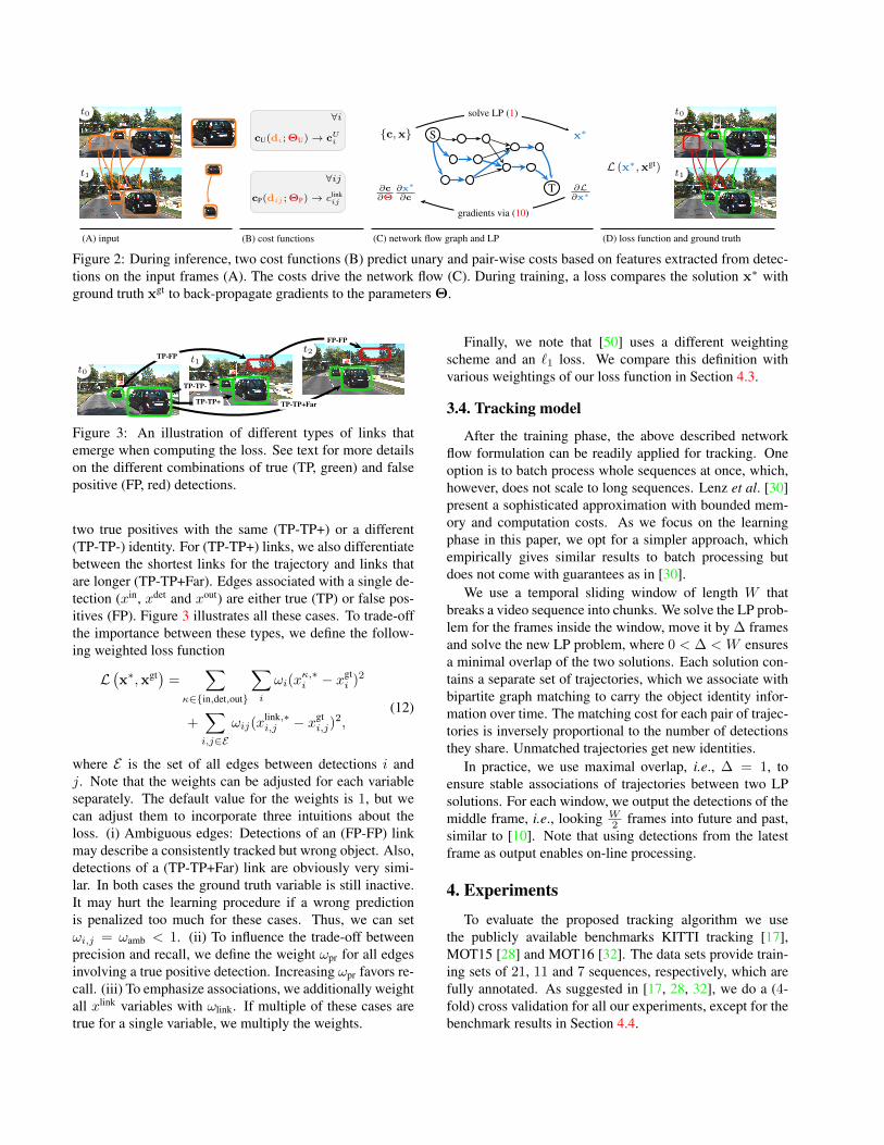
Figure 2: During inference, two cost functions (B) predict unary and pair-wise costs based on features extracted from detec-tions on the input frames (A). The costs drive the network flow (C). During training, a loss compares the solution x∗ withground truth xgt to back-propagate gradients to the parameters Θ.

t0t1

t2FP-FP

TP-FP

TP-TP-

TP-TP+ TP-TP+Far

Figure 3: An illustration of different types of links thatemerge when computing the loss. See text for more detailson the different combinations of true (TP, green) and falsepositive (FP, red) detections.

two true positives with the same (TP-TP+) or a different(TP-TP-) identity. For (TP-TP+) links, we also differentiatebetween the shortest links for the trajectory and links thatare longer (TP-TP+Far). Edges associated with a single de-tection (xin, xdet and xout) are either true (TP) or false pos-itives (FP). Figure 3 illustrates all these cases. To trade-offthe importance between these types, we define the follow-ing weighted loss function

L(x∗,xgt) =

∑κ∈{in,det,out}

∑i

ωi(xκ,∗i − xgt

i )2

+∑i,j∈E

ωij(xlink,∗i,j − xgt

i,j)2,

(12)

where E is the set of all edges between detections i andj. Note that the weights can be adjusted for each variableseparately. The default value for the weights is 1, but wecan adjust them to incorporate three intuitions about theloss. (i) Ambiguous edges: Detections of an (FP-FP) linkmay describe a consistently tracked but wrong object. Also,detections of a (TP-TP+Far) link are obviously very simi-lar. In both cases the ground truth variable is still inactive.It may hurt the learning procedure if a wrong predictionis penalized too much for these cases. Thus, we can setωi,j = ωamb < 1. (ii) To influence the trade-off betweenprecision and recall, we define the weight ωpr for all edgesinvolving a true positive detection. Increasing ωpr favors re-call. (iii) To emphasize associations, we additionally weightall xlink variables with ωlink. If multiple of these cases aretrue for a single variable, we multiply the weights.

Finally, we note that [50] uses a different weightingscheme and an `1 loss. We compare this definition withvarious weightings of our loss function in Section 4.3.

3.4. Tracking model

After the training phase, the above described networkflow formulation can be readily applied for tracking. Oneoption is to batch process whole sequences at once, which,however, does not scale to long sequences. Lenz et al. [30]present a sophisticated approximation with bounded mem-ory and computation costs. As we focus on the learningphase in this paper, we opt for a simpler approach, whichempirically gives similar results to batch processing butdoes not come with guarantees as in [30].

We use a temporal sliding window of length W thatbreaks a video sequence into chunks. We solve the LP prob-lem for the frames inside the window, move it by ∆ framesand solve the new LP problem, where 0 < ∆ < W ensuresa minimal overlap of the two solutions. Each solution con-tains a separate set of trajectories, which we associate withbipartite graph matching to carry the object identity infor-mation over time. The matching cost for each pair of trajec-tories is inversely proportional to the number of detectionsthey share. Unmatched trajectories get new identities.

In practice, we use maximal overlap, i.e., ∆ = 1, toensure stable associations of trajectories between two LPsolutions. For each window, we output the detections of themiddle frame, i.e., looking W

2 frames into future and past,similar to [10]. Note that using detections from the latestframe as output enables on-line processing.

4. Experiments

To evaluate the proposed tracking algorithm we usethe publicly available benchmarks KITTI tracking [17],MOT15 [28] and MOT16 [32]. The data sets provide train-ing sets of 21, 11 and 7 sequences, respectively, which arefully annotated. As suggested in [17, 28, 32], we do a (4-fold) cross validation for all our experiments, except for thebenchmark results in Section 4.4.

To assess the performance of the tracking algorithmswe rely on standard MOT metrics, CLEAR MOT [4] andMT/PT/ML [31], which are also used by both bench-marks [17, 28]. This set of metrics measures recall and pre-cision, both on a detection and trajectory level, counts thenumber of identity switches and fragmentations of trajecto-ries and also provides an overall tracking accuracy (MOTA).

4.1. Learned versus hand-crafted cost functions

The main contribution of this paper is a novel way to au-tomatically learn parameterized cost functions for a networkflow based tracking model from data. We illustrate the effi-cacy of the learned cost functions by comparing them withtwo standard choices for hand-crafted costs. First, we fol-low [29] and define cdet

i = log(1 − p(di)), where p(di) isthe detection probability, and

clinki,j = − log E

(‖b(di)− b(dj)‖

∆t, Vmax

)− log(B∆t−1),

(13)where E(Vt, Vmax) = 1

2 + 12 erf(−Vt+0.5·Vmax

0.25·Vmax) with erf(·) be-

ing the Gauss error function and ∆t is the frame differencebetween i and j. While [29] defines a slightly different net-work flow graph, we keep the graph definition the same (seeSection 3.1) for all methods to ensure a fair comparison ofthe costs. Second, we hand-craft our own cost function anddefine cdet

i = α · p(di) as well as

clinki,j = (1− IoU(b(di),b(dj))) + β · (∆t − 1), (14)

where IoU(·, ·) is the intersection over union. We tuneall parameters, i.e., cin

i = couti = C (we did not observe

any benefit when choosing these parameters separately), B,Vmax, α and β, with grid search to maximize MOTA whilebalancing recall. Note that the exponential growth of thesearch space w.r.t. the number of parameters makes gridsearch infeasible at some point.

With the same source of input information, i.e., bound-ing boxes b(d) and detection confidences p(d), we trainvarious types of parameterized functions with the algorithmproposed in Section 3.2. For unary costs, we use the sameparameterization as for the hand-crafted model, i.e., con-stants for cin and cout and a linear model for cdet. However,for the pair-wise costs, we evaluate a linear model, a one-layer MLP with 64 hidden neurons and a two-layer MLPwith 32 hidden neurons in both layers. The input feature fis the difference between the two bounding boxes, their de-tection confidences, the normalized time difference, as wellas the IoU value. We train all three models for 50k itera-tions using ADAM [24] with a learning rate of 10−4, whichwe decrease by a factor of 10 every 20k iterations.

Table 1 shows that our proposed training algorithm cansuccessfully learn cost functions from data on both KITTI-Tracking and MOT16 data sets. With the same input in-formation given, our approach even slightly outperforms

MOTA REC PREC MT IDS FRAG

Crafted [29] 73.64 83.54 92.99 58.73 121 459Crafted-ours 73.75 83.92 92.65 59.44 89 431

Linear 73.51 83.47 92.99 59.08 132 430MLP 1 74.09 83.93 92.87 59.61 70 371MLP 2 74.19 84.07 92.85 59.96 70 376

(a)

MOTA REC PREC MT IDS FRAG

Crafted [29] 28.28 29.94 95.04 5.80 111 1063Crafted-ours 29.19 34.01 87.88 6.77 142 1272

Linear 28.25 38.01 80.09 9.67 342 1620MLP 1 31.05 37.51 85.81 8.32 282 1553MLP 2 31.10 37.53 85.88 8.51 289 1562

(b)

Table 1: Learned vs. hand-crafted cost functions on a cross-validation on (a) KITTI-Tracking [17] and (b) MOT16 [32].

both hand-crafted baselines in terms of MOTA. In particu-lar, we observe lower identity switches and fragmentationson KITTI-Tracking and higher recall and mostly-tracked onMOT16. While our hand-crafted function (14) is inherentlylimited when objects move fast and IoU becomes 0 (com-pared to (13) [29]), both still achieve similar performance.For both baselines, we did a hierarchical grid search to getgood results. However, an even finer grid search would berequired to achieve further improvements. The attraction ofour method is that it obviates the need for such a tedioussearch and provides a principled way of finding good pa-rameters. We can also observe from the tables that non-linear functions (MLP 1 and MLP 2) perform better thanlinear functions (Linear), which is not possible in [49].

4.2. Combining multiple input sources

Recent works have shown that temporal and appearancefeatures are often beneficial for MOT. Choi [10] presents aspatio-temporal feature (ALFD) to compare two detections,which summarizes statistics from tracked interest points ina 288-dimensional histogram. Leal-Taixe et al. [27] showhow to use raw RGB data with a Siamese network to com-pute an affinity metric for pedestrian tracking. Incorpo-rating such information into a tracking model typically re-quires (i) an isolated learning phase for the affinity metricand (ii) some hand-tuning to combine it with other affinitymetrics and other costs in the model (e.g., cin, cdet, cout). Inthe following, we demonstrate the use of both motion andappearance features in our framework.

Motion-features: In Table 2, we demonstrate the im-pact of the motion feature ALFD [10] compared to purelyspatial features on the KITTI-Tracking data set as in [10].For each source of input, we compare both hand-crafted(C) and learned (L) pair-wise cost functions. First, we use

Inputs MOTA REC PREC MT IDS FRAG

(C) B 73.64 83.54 92.99 58.73 121 459(L) B 73.65 84.55 92.00 61.55 89 422

(C) B+O 73.75 83.92 92.65 59.44 89 431(L) B+O 74.12 84.13 92.69 60.49 55 361

(C) B+O+M 73.07 85.07 90.92 61.73 43 386(L) B+O+M 74.11 84.74 92.05 61.73 29 335

Table 2: We evaluate the influence of different types of inputsources, raw detection inputs (B), bounding box overlaps(O) and the ALFD motion feature [10] (M) for both learned(L) and hand-crafted (C) costs on KITTI-Tracking [17].

only the raw bounding box information (B), i.e., locationand temporal difference and detection score. For the hand-crafted baseline, we use the cost function defined in (13),i.e., [29]. Second, we add the IoU overlap (B+O) and use(14) for the hand-crafted baseline. Third, we incorporateALFD [10] into the cost (B+O+M). To build a hand-craftedbaseline for (B+O+M), we construct a separate training setof ALFD features containing examples for positive and neg-ative matches and train an SVM on the binary classificationtask. During tracking, the normalized SVM scores sA (asigmoid function maps the raw SVM scores into [0, 1]) areincorporated into the cost function

clinki,j = (1−IoU(b(di),b(dj)))+β ·(∆t−1)+γ ·(1− sA),

(15)where γ is another hyper-parameter we also tune with grid-search. For our learned cost functions, we use a 2-layerMLP with 64 neurons in each layer to predict clink

i,j for the(B) and (B+O) options. For (B+O+M), we use a separate 2-layer MLP to process the 288-dimensional ALFD feature,concatenate both 64-dimensional hidden vectors of the sec-ond layers, and predict clink

i,j with a final linear layer.Table 2 again shows that learned cost functions outper-

form hand-crafted costs for all input sources, which is con-sistent with the previous experiment in Section 4.1. The ta-ble also demonstrates the ability of our approach to make ef-fective use of the ALFD motion feature [10], especially foridentity switches and fragmentations. While it is typicallytedious and suboptimal to combine such diverse featuresin hand-crafted cost functions, it is easy with our learningmethod because all parameters can still be jointly trainedunder the same loss function.

Appearance features: Here, we investigate the impactof raw RGB data on both unary and pair-wise costs of thenetwork flow formulation. We use the MOT15 data set [28]and the provided ACF detections [14]. First, we integratethe raw RGB data into the unary cost cdet

i (Au). For eachdetected bounding box b(di), we crop the underlying RGBpatch Ii with a fixed aspect ratio, resize the patch to 128×64

Unary cost MOTA REC PREC MT IDS FRAG

Crafted [29] 30.55 38.54 83.70 11.60 194 853Crafted-ours 30.43 38.98 82.69 11.40 156 825(B+O) 28.94 43.63 75.47 14.00 204 962Au+(B+O) 39.08 46.99 86.71 15.60 285 1062Au+(B+O+Ap) 39.23 47.17 86.50 15.80 233 954

Table 3: Using appearance for unary (Au) and pair-wise(Ap) cost functions clearly improves tracking performance.

0 10k 20k 30k 40k 50k

2

4

6

8

10

Los

s

(B+O)Au+(B+O)Au+(B+O+Ap)

0 10k 20k 30k 40k 50k6

7

8

9

10

Los

s

Figure 4: The difference in the loss on the training (left)and validation set (right) over 50k iterations of training formodels w/ (Au,Ap) and w/o appearance features.

and define the cost

cdeti = cconf(p(di); Θconf) + cAu(Ii; ΘAu), (16)

which consists of one linear function taking the detectionconfidence and one deep network taking the image patch.We choose ResNet-50 [19] to extract features for cAu butany other differentiable function can be used as well.

Second, we use a Siamese network (same as for unaryterm) that compares RGB patches of two detections, sim-ilar to [27] but without optical flow information. As withthe motion features above, we use a two-stream networkto combine spatial information (B+O) with appearance fea-tures (Ap). The hidden feature vector of a 2-layer MLP(B+O) is concatenated with the difference of the hidden fea-tures from the Siamese network. A final linear layer predictsthe costs clink

i,j of the pair-wise terms.Table 3 shows that integrating RGB information into the

detection cost Au+(B+O) improves tracking performancesignificantly over the baselines. Using the RGB informa-tion in the pair-wise cost as well Au+(B+O+Ap) further im-proves results, especially for identity switches and fragmen-tations. Figure 4 visualizes the loss on the training and vali-dation set for the three learning-based methods, which againshows the impact of appearance features. Note, however,that the improvement is limited because we still rely on theunderlying ACF detector and are not able to improve recallover the recall of the detector. But the experiment clearlyshows the potential ability to integrate deep network basedobject detectors directly into an end-to-end tracking frame-work. We plan to investigate this avenue in future work.

Weighting MOTA REC PREC MT IDS FRAG

none 74.07 82.84 93.78 57.67 53 333[49] 73.99 82.90 93.63 57.32 43 331none-`1 73.90 83.43 93.17 58.73 77 362[49]-`1 73.92 83.19 93.38 58.73 71 357

ωbasic = 0.1 74.15 84.11 92.72 60.49 51 360ωbasic = 0.5 74.13 83.90 92.92 59.96 62 363

ωpr = 0.3 66.84 70.68 98.35 28.92 34 216ωpr = 1.5 73.28 85.52 90.85 63.49 80 387

ωlinks = 1.5 74.14 84.53 92.31 61.38 45 357ωlinks = 2.0 74.10 84.80 92.03 61.38 42 358

Table 4: Differently weighting the loss function provides atrade-off between various behaviors of the learned costs.

4.3. Weighting the loss function

For completeness, we also investigate the impact of dif-ferent weighting schemes for the loss function defined inSection 3.3. First, we compare our loss function withoutany weighting (none) with the loss defined in [49]. We alsodo this for an `1 loss. We can see from the first part inTable 4 that both achieve similar results but [49] achievesslightly better identity switches and fragmentations. By de-creasing ωbasic we limit the impact of ambiguous cases (seeSection 3.3) and can observe a slight increase in recall andmostly tracked. Also, we can influence the trade-off be-tween precision and recall with ωpr and we can lower thenumber of identity switches by increasing ωlinks.

4.4. Benchmark results

Finally, we evaluate our learned cost functions on thebenchmark test sets. For KITTI-Tracking [17], we traincost functions equal to the ones described in Section 4.2with ALFD motion features [10], i.e., (B+O+M) in Table 2.We train the models on the full training set and upload theresults on the benchmark server. Table 5 compares ourmethod with other off-line approaches that use RegionLetdetections [51]. While [10] achieves better results on thebenchmark, their approach includes a complex graphicalmodel and a temporal model for trajectories. The fair com-parison is with Wang and Fowlkes [50], which is the mostsimilar approach to ours. While we achieve better MOTA,it is important to note that the comparison needs to be takenwith a grain of salt. We include motion features in the formof ALFD [10]. On the other hand, the graph in [50] is morecomplex as it also accounts for trajectory interactions.

We also evaluate on the MOT15 data set [28], wherewe choose the model that integrates raw RGB data intothe unary costs, i.e., Au+(B+O) in Table 3. We achievean MOTA value of 26.8, compared to 25.2 for [50] (mostsimilar model) and 29.0 for [27] (using RGB data for pair-wise term). We again note that [27] additionally integratesoptical flow into the pair-wise term. The impact of RGB

Method MOTA MOTP MT ML IDS FRAG

[30] 60.84 78.55 53.81 7.93 191 966[10] 69.73 79.46 56.25 12.96 36 225[34] 55.49 78.85 36.74 14.02 323 984[50] 66.35 77.80 55.95 8.23 63 558Ours 67.36 78.79 53.81 9.45 65 574

Table 5: Results on KITTI-Tracking [17] from 11/04/16.

t0

t1

t2

t3

t0

t1

t2

t3

Figure 5: A qualitative example showing a failure case ofthe hand-crafted costs (left) compared to the learned costs(right), which leads to a fragmentation. The green dottedboxes are ground truth, the solid colored are ones trackedobjects. The numbers are the object IDs. Best viewed incolor and zoomed.

features is not as pronounced as in our cross-validation ex-periment in Table 3. The most likely reason we found forthis scenario is over-fitting of the unary terms.

Figure 5 also gives a qualitative comparison betweenhand-crafted and learned cost functions on KITTI [17]. Thesupplemental material contains more qualitative results.

5. ConclusionOur work demonstrates how to learn a parameterized

cost function of a network flow problem for multi-objecttracking in an end-to-end fashion. The main benefit is thegained flexibility in the design of the cost function. We onlyassume it to be parameterized and differentiable, enablingthe use of powerful neural network architectures. Our for-mulation learns the costs of all variables in the networkflow graph, avoiding the delicate task of hand-crafting thesecosts. Moreover, our approach also allows for easily com-bining different sources of input data. Evaluations on threepublic data sets confirm these benefits empirically.

For future works, we plan to integrate object detectorsend-to-end into this tracking model, investigate more com-plex network flow graphs with trajectory interactions andexplore applications to max-flow problems.

References[1] A. Andriyenko, K. Schindler, and S. Roth. Discrete-

Continuous Optimization for Multi-Target Tracking. InCVPR, 2012. 2

[2] S.-H. Bae and K.-J. Yoon. Robust Online Multi-ObjectTracking based on Tracklet Confidence and Online Discrim-inative Appearance Learning. In CVPR, 2014. 2

[3] J. Berclaz, F. Fleuret, E. Turetken, and P. Fua. Multiple Ob-ject Tracking using K-Shortest Paths Optimization. PAMI,33(9):1806–1819, 2011. 1, 2

[4] K. Bernardin and R. Stiefelhagen. Evaluating Multiple Ob-ject Tracking Performance: The CLEAR MOT Metrics.EURASIP Journal on Image and Video Processing, 2008. 6

[5] S. Boyd and L. Vandenberghe. Convex Optimization. Cam-bridge University Press, 2004. 3, 4

[6] J. Bracken and J. T. McGill. Mathematical Programs withOptimization Problems in the Constraints. Operations Re-search, 21:37–44, 1973. 1, 2

[7] M. D. Breitenstein, F. Reichlin, B. Leibe, E. Koller-Meier,and L. Van Gool. Robust Tracking-by-Detection using a De-tector Confidence Particle Filter. In ICCV, 2009. 1, 2

[8] M. D. Breitenstein, F. Reichlin, B. Leibe, E. Koller-Meier,and L. Van Gool. Online Multiperson Tracking-by-Detectionfrom a Single, Uncalibrated Camera. PAMI, 33(9):1820–1833, 2011. 2

[9] A. A. Butt and R. T. Collins. Multi-target Tracking by La-grangian Relaxation to Min-Cost Network Flow. 2013. 2

[10] W. Choi. Near-Online Multi-target Tracking with Aggre-gated Local Flow Descriptor. In ICCV, 2015. 1, 2, 3, 5,6, 7, 8

[11] W. Choi, C. Pantofaru, and S. Savarese. A General Frame-work for Tracking Multiple People from a Moving Camera.PAMI, 35(7):1577–1591, 2013. 2

[12] W. Choi and S. Savarese. A Unified Framework for Multi-Target Tracking and Collective Activity Recognition. InECCV, 2012. 2

[13] B. Colson, P. Marcotte, and G. Savard. An overviewof bilevel optimization. Annals of Operations Research,153(1):235–256, 2007. 1, 2

[14] P. Dollar, R. Appel, S. Belongie, and P. Perona. Fast FeaturePyramids for Object Detection. PAMI, 36(8):1532–1545,2014. 7

[15] A. Ess, B. Leibe, K. Schindler, and L. van Gool. Ro-bust Multi-Person Tracking from a Mobile Platform. PAMI,31(10):1831–1846, 2009. 1, 2

[16] P. F. Felzenszwalb, R. B. Girshick, D. McAllester, and D. Ra-manan. Object Detection with Discriminatively Trained PartBased Models. PAMI, 32(9):1627–1645, 2010. 1

[17] A. Geiger, P. Lenz, and R. Urtasun. Are we ready for Au-tonomous Driving? The KITTI Vision Benchmark Suite. InCVPR, 2012. 1, 5, 6, 7, 8

[18] N. J. Gordon, D. Salmond, and A. Smith. Novel approachto nonlinear/non-Gaussian Bayesian state estimation. IEEProceedings F (Radar and Signal Processing), 140:107–113,1993. 2

[19] K. He, X. Zhang, S. Ren, and J. Sun. Deep Residual Learningfor Image Recognition. In CVPR, 2016. 7

[20] C. Huang, B. Wu, and R. Nevatia. Robust Object Tracking byHierarchical Association of Detection Responses. In ECCV,2008. 2

[21] R. E. Kalman. A new approach to linear filtering and predic-tion problems. Transactions of the ASME–Journal of BasicEngineering, 82(Series D):35–45, 1960. 2

[22] Z. Khan, T. Balch, and F. Dellaert. MCMC-Based ParticleFiltering for Tracking a Variable Number of Interacting Tar-gets. PAMI, 27(11):1805–1819, 2005. 1

[23] S. Kim, S. Kwak, J. Feyereisl, and B. Han. Online Multi-Target Tracking by Large Margin Structured Learning. InACCV, 2012. 2

[24] D. P. Kingma and J. Ba. Adam: A Method for StochasticOptimization. In ICLR, 2015. 6

[25] H. W. Kuhn. The Hungarian Method for the AssignmentProblem. Naval Research Logistics Quarterly, 2:83–97,1955. 1, 2

[26] C.-H. Kuo, C. Huang, and R. Nevatia. Multi-Target Trackingby On-Line Learned Discriminative Appearance Models. InCVPR, 2010. 1, 2

[27] L. Leal-Taixe, C. Canton-Ferrer, and K. Schindler. Learn-ing by tracking: Siamese CNN for robust target association.In DeepVision: Deep Learning for Computer Vision, CVPRWorkshop, 2016. 1, 2, 6, 7, 8

[28] L. Leal-Taixe, A. Milan, I. Reid., S. Roth, and K. Schindler.MOTChallenge 2015: Towards a Benchmark for Multi-Target Tracking. arXiv:1504.01942, 2015. 1, 5, 6, 7, 8

[29] L. Leal-Taixe, G. Pons-Moll, and B. Rosenhahn. Everybodyneeds somebody: Modeling social and grouping behavior ona linear programming multiple people tracker. 2011. 1, 2, 6,7

[30] P. Lenz, A. Geiger, and R. Urtasun. FollowMe: EfficientOnline Min-Cost Flow Tracking with Bounded Memory andComputation. In ICCV, 2015. 2, 5, 8

[31] Y. Li, C. Huang, and R. Nevatia. Learning to Associate:HybridBoosted Multi-Target Tracker for Crowded Scene. InCVPR, 2009. 1, 2, 6

[32] A. Milan, L. Leal-Taixe, I. Reid, S. Roth, and K. Schindler.MOT16: A Benchmark for Multi-Object Tracking.arXiv:1603.00831, 2016. 1, 5, 6

[33] A. Milan, S. Roth, and K. Schindler. Continuous EnergyMinimization for Multitarget Tracking. PAMI, 36(1):58–72,2014. 1, 2

[34] A. Milan, K. Schindler, and S. Roth. Detection- andTrajectory-Level Exclusion in Multiple Object Tracking. InCVPR, 2013. 8

[35] J. Munkres. Algorithms for the Assignment and Transporta-tion Problems. Journal of the Society for Industrial and Ap-plied Mathematics, 5(1):32–38, 1957. 1, 2

[36] P. Ochs, R. Ranftl, T. Brox, and T. Pock. Bilevel Opti-mization with Nonsmooth Lower Level Problems. In SSVM,2015. 4

[37] S. Oh, S. Russell, and S. Sastry. Markov Chain Monte CarloData Association for Multiple-Target Tracking. IEEE Trans-actions on Automatic Control, 54(3):481–497, 2009. 1

[38] K. Okuma, A. Taleghani, N. De Freitas, J. J. Little, and D. G.Lowe. A Boosted Particle Filter: Multitarget Detection andTracking. In ECCV, 2004. 1

[39] S. Pellegrini, A. Ess, K. Schindler, and L. van Gool. YoullNever Walk Alone: Modeling Social Behavior for Multi-target Tracking. In ICCV, 2009. 2

[40] H. Pirsiavash, D. Ramanan, and C. C. Fowlkes. Globally-Optimal Greedy Algorithms for Tracking a Variable Numberof Objects. In CVPR, 2011. 2

[41] H. Possegger, T. Mauthner, P. M. Roth, and H. Bischof.Occlusion Geodesics for Online Multi-Object Tracking. InCVPR, 2014. 1, 2

[42] R. Ranftl and T. Pock. A Deep Variational Model for ImageSegmentation. In GCPR, 2014. 2

[43] S. Ren, K. He, R. Girshick, and J. Sun. Faster R-CNN: To-wards real-time object detection with region proposal net-works. In NIPS, 2015. 1

[44] G. Riegler, R. Ranftl, M. Ruther, T. Pock, and H. Bischof.Depth Restoration via Joint Training of a Global RegressionModel and CNNs. In BMVC, 2015. 2

[45] G. Riegler, M. Ruther, and H. Bischof. ATGV-Net: AccurateDepth Super-Resolution. In ECCV, 2016. 2

[46] F. Solera, S. Calderara, and R. Cucchiara. Learning to Divideand Conquer for Online Multi-Target Tracking. In CVPR,2015. 2

[47] X. Song, J. Cui, H. Zha, and H. Zhao. Vision-based MultipleInteracting Targets Tracking via On-line Supervised Learn-ing. In ECCV, 2008. 2

[48] I. Tsochantaridis, T. Joachims, T. Hofmann, and Y. Altun.Large Margin Methods for Structured and InterdependentOutput Variables. JMLR, 6:1453–1484, 2005. 2

[49] S. Wang and C. Fowlkes. Learning Optimal Parameters ForMulti-target Tracking. In BMVC, 2015. 1, 2, 6, 8

[50] S. Wang and C. Fowlkes. Learning Optimal Parameters forMulti-target Tracking with Contextual Interactions. IJCV,pages 1–18, 2016. 1, 4, 5, 8

[51] X. Wang, M. Yang, S. Zhu, and Y. Lin. Regionlets forGeneric Object Detection. In ICCV, 2013. 1, 8

[52] Y. Xiang, A. Alahi, and S. Savarese. Learning to Track: On-line Multi-Object Tracking by Decision Making. In ICCV,2015. 1

[53] A. R. Zamir, A. Dehghan, and M. Shah. GMCP-Tracker:Global Multi-object Tracking Using Generalized MinimumClique Graphs. In ECCV, 2012. 2

[54] L. Zhang, Y. Li, and R. Nevatia. Global Data Associationfor Multi-Object Tracking Using Network Flows. In CVPR,2008. 1, 2, 3