Full Terms & Conditions of access and use can be found athttps://www.tandfonline.com/action/journalInformation?journalCode=ujqt20

Journal of Quality TechnologyA Quarterly Journal of Methods, Applications and Related Topics

ISSN: (Print) (Online) Journal homepage: https://www.tandfonline.com/loi/ujqt20

Deep multistage multi-task learning for qualityprediction of multistage manufacturing systems

Hao Yan, Nurettin Dorukhan Sergin, William A. Brenneman, Stephen JosephLange & Shan Ba

To cite this article: Hao Yan, Nurettin Dorukhan Sergin, William A. Brenneman, Stephen JosephLange & Shan Ba (2021): Deep multistage multi-task learning for quality prediction of multistagemanufacturing systems, Journal of Quality Technology, DOI: 10.1080/00224065.2021.1903822

To link to this article: https://doi.org/10.1080/00224065.2021.1903822

Published online: 20 Apr 2021.

Submit your article to this journal

Article views: 61

View related articles

View Crossmark data

Deep multistage multi-task learning for quality prediction of multistagemanufacturing systems

Hao Yana , Nurettin Dorukhan Sergina, William A. Brennemanb, Stephen Joseph Langeb�, and Shan Bab�aThe School of Computing, Informatics, and Decision Systems Engineering, Arizona State University, Tempe, Arizona; bProcter andGamble Company, Cincinnati, Ohio

ABSTRACTIn multistage manufacturing systems, modeling multiple quality indices based on the pro-cess sensing variables is important. However, the classic modeling technique predicts eachquality variable one at a time, which fails to consider the correlation within or betweenstages. We propose a deep multistage multi-task learning framework to jointly predict alloutput sensing variables in a unified end-to-end learning framework according to thesequential system architecture in the MMS. Our numerical studies and real case study haveshown that the new model has a superior performance compared to many benchmarkmethods as well as great interpretability through developed variable selection techniques.

KEYWORDSdeep neural network;multistage manufacturingprocess; multi-task learning;quality prediction

1. Introduction

A Multistage Manufacturing System (MMS) refers toa system consisting of multiple stages (e.g., units, sta-tions, or operations) to fabricate a final product. Inmost cases, an MMS has a sequential configurationthat links all stages with a directed flow from the ini-tial part/material to the final product. In an MMS,massive data are collected from the in-situ multivari-ate sensing of process variables and the product qual-ity measurements from intermediate stages and thefinal stage. It is challenging to model the MMS datadue to the following characteristics: 1) Multiple corre-lated output variables: The MMS can have hundredsof output sensing variables at different stages thatmeasure different quality attributes of the product indifferent stages. These quality responses are often cor-related and evolve together with the product in theMMS. 2) High dimensional input variables: In anMMS, there can be hundreds of input variables (e.g.,process sensors) in each stage as well as a large numberof stages/stations. 3) Complex sequential dependencybetween stages and sensor measurements: The productquality from an MMS is determined by complex inter-actions among multiple stages. For example, the qualitycharacteristics of one stage are not only influenced bylocal process variations within that stage, but also bythe variation propagated from upstream stages.

The methodology developed in this paper is moti-vated by a diaper manufacturing system, which iscomposed of several sequential converting processsteps with associated equipment components, whichare controlled through many process factors. The set-points for these factors and their variation may affectthe reliability of the process and the quality of theproduct produced by it. Performance data of the con-verting equipment, as well as in-process product qual-ity measures, are collected and stored by sensors andhigh-speed cameras installed on the production line.The time-series data may be high-frequency data(sampled every several milliseconds over seconds orminutes) and/or low-frequency data (samples collectedon a one-minute frequency over months). Thenumber of variables in this MMS is in the range of500-1000. This data is used to detect abnormal per-formance early enough to prevent machine stops,quality degradation or scrap from rejected defectiveproducts. To model the variation propagation of theentire MMS, the stream of variation (SoV) theory wasproposed to model the variation propagation in anMMS (Shi 2006). For example, when one of the stagesof the multistage system experiences a malfunction,SoV can be used to model the consequence of such achange on the final product (Li and Tsung 2009;Lawless, Mackay, and Robinson 1999; Jin and Tsung

CONTACT Hao Yan haoyan@asu.edu Arizona State University, Tempe, AZ 85287.�At the time of submission, Shan Ba was affiliated with Procter and Gamble Co. in Cincinnati, Ohio, but is now affiliated with LinkedIn Corporation. Also atthe time of submission, Stephen Joseph Lange was affiliated with Procter and Gamble Co. in Cincinnati, Ohio, but is now affiliated with ProcessDev, LLC.� 2021 American Society for Quality

JOURNAL OF QUALITY TECHNOLOGYhttps://doi.org/10.1080/00224065.2021.1903822

2009). However, in modern manufacturing processes,such as semiconductor manufacturing or diaper man-ufacturing process, it is often not easy to define thesystem state explicitly due to the complex systemmechanism. In conclusion, since classic approachesassume the design information and physical law of theprocess to be perfectly known, these classicalapproaches cannot be used for complex systems withunknown engineering or science knowledge.

In industrial practice and literature, to deal withmore complicated types of data and nonlineardependencies, predictive modeling techniques areoften used. However, these models are typicallydesigned based on a single output variable such asdecision tree (Bak Ir et al. 2006; Jemwa and Aldrich2005) or neural network (Zhou et al. 2006; Tam et al.2004; Chang and Jiang 2002) and have the followingmajor limitations: 1) Due to the independent model-ing of each output variable at each stage, the correl-ation between each output variable is not considered.2) Due to the need to have one model for every singlevariable, it lacks a unified way of modeling the MMSand variation propagation throughout the system.Hundreds or even thousands of independent modelsare needed, which is very hard to train and deploy. Inaddition, this greatly increases the number of parame-ters in modeling the entire MMS, which could lead tosevere over-fitting when the number of samples islimited. 3) Due to the need for a unified model forprocess monitoring and control, there may be trade-offs between different output variables (e.g., qualityvariables). A joint modeling framework can be usedfor process optimization of multiple input variables,considering the tradeoffs between different output var-iables simultaneously.

To address the aforementioned challenges, we aimto develop a data-driven approach, namely the deepmultistage multi-task learning (DMMTL) framework,to link all the input and output variables in a sequen-tial MMS. To the best of the authors’ knowledge, thisis the first end-to-end system-level predictive modelingframework in modeling all input and output variablesjointly in an MMS. The proposed framework uses alatent state representation similar to the SoV model,but instead of specifying the hidden state representa-tion manually, the proposed framework aims to learnthe latent state representation and how it propagatesthrough the MMS in an end-to-end fashion throughall the output variables simultaneously. We furthermake many improvements on the model architectureto model the MMS, such as an independent state tran-sition model and the group lasso penalty. Finally, since

model interpretability and diagnostics are also import-ant, we will also demonstrate how the proposedDMMTL is able to rank the most important inputvariables according to each output variable for systemdiagnostics.

To model multiple output variables simultaneously,the proposed DMMTL is also inspired by the recentdevelopment in multi-task learning (MTL). MTL is asub-field of statistical machine learning in which mul-tiple correlated learning tasks are solved at the sametime while exploiting the commonalities across taskswhile modeling their differences (Caruana 1997). Theproposed DMMTL can benefit through incorporatingthe use of MTL to jointly model all output variablesfrom all stages simultaneously since these output vari-ables often measure correlated attributes of the sameproduct in the MMS. However, MTL by itself canonly be used for joint modeling of multiple sensingvariables within the same stage, which fails to modelthe out variables with sequential order.

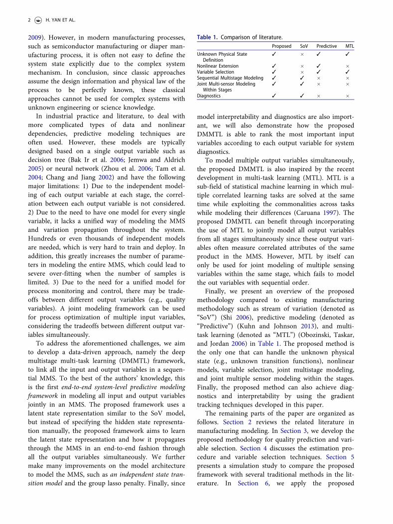
Finally, we present an overview of the proposedmethodology compared to existing manufacturingmethodology such as stream of variation (denoted as“SoV”) (Shi 2006), predictive modeling (denoted as“Predictive”) (Kuhn and Johnson 2013), and multi-task learning (denoted as “MTL”) (Obozinski, Taskar,and Jordan 2006) in Table 1. The proposed method isthe only one that can handle the unknown physicalstate (e.g., unknown transition functions), nonlinearmodels, variable selection, joint multistage modeling,and joint multiple sensor modeling within the stages.Finally, the proposed method can also achieve diag-nostics and interpretability by using the gradienttracking techniques developed in this paper.

The remaining parts of the paper are organized asfollows. Section 2 reviews the related literature inmanufacturing modeling. In Section 3, we develop theproposed methodology for quality prediction and vari-able selection. Section 4 discusses the estimation pro-cedure and variable selection techniques. Section 5presents a simulation study to compare the proposedframework with several traditional methods in the lit-erature. In Section 6, we apply the proposed

Table 1. Comparison of literature.Proposed SoV Predictive MTL

Unknown Physical StateDefinition

� � � �

Nonlinear Extension � � � �Variable Selection � � � �Sequential Multistage Modeling � � � �Joint Multi-sensor Modeling

Within Stages� � � �

Diagnostics � � � �

2 H. YAN ET AL.

framework to model a diaper manufacturing line. InSection 7, we provide concluding remarks and futuredirection. For a more detailed comparison of the pro-posed method with SoV, please refer to Appendix A.

2. Literature review

In this section, we will review the related literature inthe modeling of manufacturing systems. We brieflyclassify existing techniques into two types, single-stagemodeling and multistage modeling.

Single-stage models typically focus on process mon-itoring (Joe Qin 2003; Kourti, Lee, and Macgregor1996; MacGregor and Kourti 1995) and the prediction(Hao et al. 2017; Jin, Li, and Shi 2007) of sensing vari-ables observed in the same stage of the manufacturingsystem. For process monitoring, uni-variate (Shewhart1931), multivariate (Lowry and Montgomery 1995),profile-based (Woodall 2007), multi-channel-profile-based (Paynabar, Jin, and Pacella 2013; Zhang et al.2020), and image-based (Yan, Paynabar, and Shi 2015,2017) process monitoring techniques are developed.For quality prediction, regression and classificationtechniques such as linear regression (Skinner et al.2002), logistic regression (Jin, Li, and Shi 2007), ten-sor learning (Yan, Paynabar, and Pacella 2018), deci-sion trees (Bak Ir et al. 2006; Jemwa and Aldrich2005), and neural network (Zhou et al. 2006; Tamet al. 2004; Chang and Jiang 2002) are applied torelate the input variables (e.g. process sensing varia-bles) with the output variables (e.g. quality sensingvariables). Despite the use of nonlinear methods andthe ability to incorporate heterogeneous high-dimen-sional data, it still lacks a unified framework for mod-eling the variation propagation among stages.

To model multistage systems, SoV has been suc-cessfully implemented in the multistage automotiveassembly process (Jin and Shi 1999; Apley and Shi1998; Ceglarek and Shi 1996; Ding et al. 2005; Shiu,Ceglarek, and Shi 1997) and machining process(Huang, Zhou, and Shi 2002; Liu, Shi, and Hu 2009;Zhou, Huang, and Shi 2003; Abellan-Nebot et al.2012). For example, SoV introduces the state spacerepresentation to quantify the system status. In a trad-itional SoV model, the state variables are definedphysically (e.g., geometry deviation of the product(Ding et al. 2005)). For a more detailed literaturereview on MMS models, please refer to (Shi 2006).There are some other techniques besides SoV thathave been developed for multistage modeling.Bayesian network techniques (Friedman, Geiger, andGoldszmidt 1997; Jensen 1996) have been proposed to

model the complex dependency between multiplemanufacturing stages for both process monitoring(Liu, Zhang, and Shi 2014; Yu and Rashid 2013; Liuand Shi 2013) and quality prediction (Reckhow 1999;Correa et al. 2008). However, these techniques assumethat the complex dependencies between multiple out-put variables are known and require the feature selec-tion techniques to be used beforehand, and thuscannot be applied to a system with unknown transi-tion and dependency. In the literature, reconfiguredpiece-wise linear regression trees are developed (Jinand Shi 2012) to take advantage of intermediate qual-ity variables and model the nonlinear relationshipbetween the sequential order of the input and outputvariables. However, this technique cannot performfeature selection for a large number of sensors and italso assumes the same quality responses are measuredin the intermediate stages. Furthermore, it optimizesthe model in a greedy stage-wise approach, whichmay suffer from local optimality. In conclusion, simi-lar to SoV, most of the techniques in the literaturefocus on either manual selection of important sensors,manual extraction of useful features transformation,and clear definition of system state and transitionbefore the MMS modeling can be applied. But thesetechniques cannot be used for quality prediction ofcomplex systems with unknown architectures (Dinget al. 2005; Apley and Shi 1998; Zhou, Huang, andShi 2003, Zhou, Chen, and Shi 2004; Ceglarek andShi 1996).

3. Methodology development

In this section, we will first define the problem settingand notations in Section 3.1 followed by our proposedDMMTL framework in Section 3.2. We furtherderived a more efficient optimization algorithm tohandle the non-smooth loss function and penalty inSection 3.3.

3.1. Problem setting and notation

We denote xk ¼ ðxk, 1, :::, xk, nx, kÞT is a vector of inputvariables (i.e. process sensing variables) in stage k,where xk, i is the ith sensing variable in stage k, andnx, k is the total number of input sensing variables instage k ¼ 1, :::,K, where K is the number of stages.We denote yk ¼ ðyk, 1, :::, yk, ny, kÞT as the output varia-bles (i.e. product quality sensing variables) in stage k,where yk, j is the jth sensing variable in stage k andny, k is the total number of output sensing variables instage k. To link multiple stages together, we introduce

JOURNAL OF QUALITY TECHNOLOGY 3

the hidden state variable hk, which is a vector to rep-resent the state of the product in stage k. For simpli-city, we assume the hidden state variable hk is of thesame dimension nh across different states. The goal ofthis research is to build a multi-task learning frame-work to predict the quality indices Y ¼ fy1, :::, yKgmeasured at different stages given X ¼ fx1, :::, xKg: Inthis section, we assume that we are only dealing withdata with sample size 1. We will discuss how toextend this to the mini-batch version utilizing mini-batch stochastic gradient descent with multiple sam-ples in Appendix D in detail.

3.2. Proposed framework

We will introduce our proposed DMMTL model tosolve the aforementioned challenges by learning thehidden state representation hk from data. Here, hkshould contain the information not only to predictthe current state output yk but also the future stageoutput yk0 with k0 > k: In kth manufacturing stage, wewill define the transition function to model the statetransition between hk�1 and hk and the emission func-tion to model the relationship between hk and yk aslearnable parametric functions with model parametershhk , h

gk as

hk ¼ fkðhk�1, xk; hhkÞ, yk ¼ gkðhk; hgkÞ þ �yk, (1)

�yk � Nð0, r2Þ: One example of such architecture islisted in (12), which we use a one-layer neural net-work to model the nonlinear state transition andemission function.

hk ¼ rðWxkxk þUhkhk�1 þ bhkÞ, yk¼ Vykhk þ bgk þ �yk, (2)

where rðxÞ ¼ 1=ð1þ exp ð�xÞÞ is the activationfunction. Define the stage transition model parametersas hhk ¼ fUhk,Wxk, bhkg: gkjð�Þ represents the emissionfunction to link the hidden variable to the outputvariable. For example, gkjð�Þ can be a linear functionwith model parameters h

gk ¼ fVyk, bgkg or nonlinear

functions such as neural networks. Here, we denotehk ¼ fhhk , hgkg as the model parameters for stage k.Furthermore, if we use one-layer neural networks forboth transition and emission, the model does sharesome similarity with RNN models. However, themajor limitation of using RNN in MMS is that differ-ent manufacturing stages are inherently different. Theunderlying physics is entirely different for each stagewhich not only results in the different transitionparameters hhk ¼ fUhk,Wxk, bhkg and emission param-eters h

gk ¼ fVyk, bgkg: RNN also assumes the same set

of variables are predicted in each time. However, inMMS, different quality inspection sensors are set upin each manufacturing stage, denoted by yk: Finally,RNN is a complicated model and can not achieveinput and output variable selection as the proposedapproach. More discussion of the relationship and dif-ferences of the one-layer version of the proposedDMMTL and RNN are shown in Appendix B.

The benefit of the proposed method is also itsultimate flexibility of plugging in any differentiablefunctions as fkð�Þ and gkð�Þ: For example, dependingon different applications, we can either use simplermodels (e.g., linear models) or more complicatedmodels (e.g., deep neural networks). As an example,two-layer transition and emission networks are shownas follows:

hk ¼ rðU2hkh

1k þ b2hkÞ, h1k ¼ rðWxkxk þ U1

hkh2k�1 þ b1hkÞ

yk ¼ V2yky

1k þ b2gk þ �yk, y1k ¼ rðV1

ykhk þ b1gkÞ(3)

In this case, the stage transition model parametersare hhk ¼ fU1

hk,U2hk,Wxk, b

1hk, b

2hkg, and the emission

parameters hgk ¼ fV1

yk,V2yk, b

1gk, b

2gkg and hk ¼ fhhk , hgkg:

In general, we can use a neural network with depthD1 to model for the transition function and a neuralnetwork with depth D2 to for the emission function.In this case, the model parameter is hk ¼fWxk, fUd

hk, bdhkgd¼1, :::,D1

, fVdykj , b

dgkgd¼1, :::D2

g: To showthe relationship of the proposed framework and thedeep neural network, we also visualized the architec-ture of the proposed methods in Figure 1. In this fig-ure, we showed a special case where only a singlelayer neural network is used for the transitionbetween the hidden variables. In this case, the numberof transition layers is exactly the number of manufac-turing stages. There are some additional layers modelsthe relationship of the input variables/output variableswith the hidden variables.

In the proposed DMMTL, instead of modelingeach Pðykjjfx1, :::, xkgÞ individually, we assume thatthe hidden state hk is learned through the model suchthat it compresses all the necessary information topredict the current stage output yk and future stageoutput yk0 for k0 > k: There are two benefits of usingthe latent variable hk rather than the original datafx1, :::, xkg : 1) Dimension reduction in the sequentialtransition model: fx1, :::, xkg is typically very high-dimension, especially for the later stages when k islarge. Here the model creates the low-dimensionalhidden state variable hk to compress all the necessaryinformation from fx1, :::, xkg: Therefore, the condi-tional probability can be compactly represented by

4 H. YAN ET AL.

Pðykjjfx1, :::, xkgÞ ¼ PðykjjhkÞ: 2) Shared representationfor multi-task learning: Here hk itself is used to pre-dict all the output variables ykj in stage k, which isespecially helpful when the output variables ykj ineach stage k are correlated. By assuming that differentoutput variables are conditionally independent giventhe hidden state variables hk, the architecture of themodel is shown in Figure 2.

The benefit of introducing this recursive structureand the hidden state representation hk is that thenegative joint log likelihood LðH;X ,YÞ can bedecomposed in each stage k and each sensor j as

LðH;X ,YÞ ¼ �XKk¼1

log Pðykjhk;HÞ

¼ �XKk¼1

Xny, kj¼1

log Pðykjjhk;HÞ

/XKk¼1

Xny, kj¼1

Lkðek;HÞ, (4)

where ekj ¼ ykj � gkjðhk;HÞ and Lkð�Þ is the negativelog-likelihood of the noise distribution. For example,for Gaussian noise, we can set Lkðek;HÞ ¼ jjekjj2: We

will discuss in more detail how to define Lkðek;HÞ inMMS. Finally, to make the model interpretable and toprevent overfitting, we propose to minimize the fol-lowing loss function:

minHLðHÞ þ RðHÞ, (5)

where H ¼ fh1, :::, hKg: LðHÞ ¼ PKk¼1 LkðhkÞ is the

likelihood loss function, RðHÞ ¼ PKk¼1 RkðhkÞ is the

regularization function. Here, RkðhkÞ and LkðhkÞ aredefined as the regularization term and the loss func-tion in stage k, which will be defined in more detaillater. Equation (5) can also be seen as a multi-layerneural network, where the architecture of the neuralnetwork structure depends on the physical layout ofthe manufacturing system. For example, each layer (ora set of layers) represents one stage of the manufac-turing system, with the emission network output theprediction of output sensing variables (i.e., qualityindices measured at each stage), and the transmissionnetwork passes the information to the next stage. Wepropose to combine the process variables xk or qualityvariables yk for all K stages in a multi-task learningframework in order to optimize hk in an end-to-end fashion.

Figure 1. Deep neural network structure for the proposed method.

JOURNAL OF QUALITY TECHNOLOGY 5

It is also interesting to compare the proposedDMMTL in Equation (5) to the independent mod-eling approach, where each output variable ykj atstage k and output j is modeled independently.Because such an independent modeling approachneeds to introduce new model parameters hkj foreach output variable j in each stage k, for a K-stagesystem with ny output sensors and nx input sensorsin each stage, it requires to have OðK2nxnyÞ modelparameters in total. These model parameters arenormally time-consuming to train and can lead tothe over-fitting problem. On the other hand, sinceour proposed framework reduces the hidden statedimension to nh using hhk , k ¼ 1, :::,K withOðKnhðnx þ nyÞÞ number of variables, which is typ-ically much smaller than OðK2nxnyÞ given nh �minðKnx,KnyÞ: Therefore, a shared representationyields a more compact representation with bettermemory efficiency.

Furthermore, we would like to propose the lossfunction Lkð�Þ and regularization RkðhkÞ in Equation(1) that leads to a better engineering interpretation. Inaddition, we use the regularized model to select keyinput variables and output variables. More specifically,we propose the group lasso penalty (Yuan and Lin2006) and robust statistics for a more interpretabletransition model, allowing us to perform input andoutput variable selection.

3.2.1. Group sparsity penaltyIn MMS, many input variables are irrelevant in rela-tion to predicting output variables. Therefore, theseinput variables should not affect the hidden states. Toselect the important sensors in each stage, we proposeto use the L2, 1 nom on WT

xk to encourage the modelto only select the most important sensors. In the lit-

erature, the L2, 1 norm is defined as jjWjj2, 1 ¼

Pi

ffiffiffiffiffiffiffiffiffiffiffiffiffiffiPj W

2ij

q, which penalizes the entire row of the

matrix W to be zero. Here, we propose to add thisL2, 1 norm on the transposed coefficient Wxk on (4),which penalizes the entire column of matrix Wxk tobe zero. In other words, if we define the ith column ofWxk is wi, xk, jjWT

xkjj2, 1 ¼P

j jjwi, xkjj:This penalty not only controls the model flexibility

but also can lead to a more interpretable result due tothe sensor selection power as follows:

RkðhkÞ ¼ kxjjWTxkjj2, 1 þ

k2jjHjj2, (6)

where jj � jj2 is the L2 norm and jjWTxkjj2, 1 tends to

penalize the entire column of Wxk to be 0. Forexample, if the ith column of Wxk is 0, the ith inputvariable of xki in stage k is not selected, which meansthis input variable xki is not important to the predic-tion of any output variables in the following stages.Furthermore, k

2 jjHjj2 is added for the general L2 pen-alty to prevent overfitting. We will discuss how toidentify the most important input variable for eachindividual output variable in Section 4. These regular-ization terms enforce that only some of the input vari-ables or hidden variables are used in the prediction,which models the weakly correlated patterns andimproves the interpretability of the model. Finally, wewill use the validation prediction error to select thebest tuning parameters kx, k and c.

3.2.2. Robust regressionThe most commonly defined loss function is the sumof square error (SSE) loss defined as LkðeÞ ¼ jjejj2:However, the proposed DMMTL is a multi-task learn-ing framework that focuses on predicting multipletasks (i.e., quality variables) simultaneously. In reality,due to the lack of sensing powers, many output varia-bles simply cannot be predicted by the input variables

Figure 2. Architecture of the proposed DMMTL.

6 H. YAN ET AL.

no matter what models we use. Using these non-inform-ative quality variables may not help or even corrupt thetraining results. Here, the goal is to derive the loss func-tion such that the model is robust to these unrelatedtasks or achieve a better balance between tasks.Therefore, we will compare the use of the Huber lossfunction LkðeÞ ¼ qðeÞ as defined in Equation (7) withthe traditional sum of square loss function.

qðeÞ ¼jjejj2 jej � c

2

cjej � c2

4jej > c

2

:

8><>:

(7)

Huber loss can be used instead of the mean-squarederror. The Huber loss function uses a linear functionwhen the difference is large which enables a morerobust estimation. Furthermore, we find that it can alsohelp the model identify and focus more directly on therelated output variables by being more robust to theunrelated output variables. We will discuss how to opti-mize the model parameters efficiently in Section 3.3.

3.3. Optimization algorithm

It is worth noting that problem (5) has a non-smoothloss function penalty such as kxjjWT

xkjj2, 1: In literature,the stochastic sub-gradient algorithm can be used tohandle the non-smooth penalty. However, the conver-gence speed of the stochastic sub-gradient algorithmis typically slow. Therefore, to address the non-smooth loss function, we propose to combine thestochastic proximal gradient algorithm and blockcoordinate algorithm for efficient optimization.

To efficiently optimize the problem, we will discussthe use of the stochastic proximal gradient as follows.First, we will first establish the equivalency of the pro-posed algorithm by introducing another set of outliervariables A ¼ fak, jgk, j: Here, ak, j represents the out-lier in stage k and sensor j. If ak, j ¼ 0, it implies thatthere is no outlier in stage k and sensor j for the cur-rent sample. However, if ak, j 6¼ 0, it implies that theoutlier occurs for this sample.

Proposition 1. Solving H in (5) will give the samesolution as solving H in (8).

minH, fakjgLðH,AÞ þ kxjjWTxkjj2, 1 þ

k2jjHjj2

þ cXk, j

jjak, jjj1, (8)

where LðH,AÞ ¼ Pk, j jjykj � gkjðhk;HÞ � akjjj2 is the

loss function, A ¼ fak, jgk, j:

It worth noting that both ykj and akj are scalar ifonly a single sample is used. However, if multiplesamples are used, ykj and akj are vectors. Please seeAppendix D for more details to generalize the pro-posed methods to the mini-batch version.

The proof relies on the equivalency of the Huberloss function and the sparse outlier decompositionand has been proved in (Mateos and Giannakis 2012).The benefit of using (8) is that RðH,AÞ is continuousand differentiable so that the back-propagation algo-rithm can be used efficiently. We will show how tohandle non-differentiable components of

Pk, j jjakjjj1

and jjWTxkjj2, 1 by using Block Coordinate algorithm to

update each set of variables A,Wxk, and H (excludingWxk) iteratively until convergence. Proposition 2shows how to solve A and Wxk, given the other varia-bles are fixed.

Proposition 2. In the tth iteration, solving akj givenH ¼ HðtÞ in (8) can be derived analytically as

aðtÞkj ¼ Sc=2ðykj � gkjðhk;HðtÞÞÞ:Given H ¼ HðtÞ and AðtÞ, the upper bound of (8),

defined as

minfwi, xkgLðHðt�1Þ,AðtÞÞþXi, k

@LðHðt�1Þ,AðtÞÞ@wi, xk

wi, xk � wðt�1Þi, xk

� �

þ L2

Xi, k

jjwi, xk � wðt�1Þi, xk jj2 þ kx

Xi, k

jjwi, xkjj2

þ k2

Xi, k

jjwi, xkjj2:

in the proximal gradient algorithm, can be solved by

wðtÞi, xk ¼ S kx

Lþkð LLþ k

ðwðt�1Þi, xk � 1

L@LðHðtÞ,AðtÞÞ

@wi, xkÞÞ:

Here, ScðxÞ ¼ sgnðxÞðjxj � cÞþ is the soft threshold-ing operator, in which sgnðxÞ is the sign function and

xþ ¼ maxðx, 0Þ: HðtÞ,AðtÞ, and wðtÞi, xk are the corre-

sponding values of the model parameters in the tth

iterations. L is the Lipschitz constance of the func-tion Lð�Þ:

The proof is given in Appendix C. The gradient@LðHðtÞ,AðtÞÞ

@wi, xkcan be computed from the back-propaga-

tion algorithm, which is detailed in Appendix D.Finally, since the loss function is differential for the

parameter ~H, defined as H excluding W ¼fWi, xkgi, k, the standard stochastic gradient algorithm

can be applied given W ¼ WðtÞ and A ¼ AðtÞ as fol-lows:

JOURNAL OF QUALITY TECHNOLOGY 7

~H ¼ ~H � c@LðH,WðtÞ,AðtÞÞ

@ ~H,

where c is the step length. Finally, the mini-batch ver-sion of the algorithm can also be derived with a sub-set of samples fXn

,Yngn2N t in iteration t. Moredetails of using stochastic optimization algorithm isalso shown in Appendix D.

The algorithm is summarized in Algorithm 1.Given the non-convex formulation of deep neural net-works, there is no guarantee that the algorithm wouldconverge to the the global optimum. However, wefind out that optimization algorithms typically per-form reasonably well. In case the training failed toconverge to a good optimum (measured by the valid-ation accuracy), the training can be restarted with anew random initialization point.

3.4. Tuning parameter selection

In this section, we would like to discuss the selectionof tuning parameters. Overall, we need to decide thefollowing tuning parameters: 1) Number of dimen-sions of the hidden vector hk: For the dimensionalityof the hidden vector hk, in principle, we can vary thenumber of neurons for hk for different stage k. Here,we would like to mention that in this paper, we usethe same dimensionality of the hidden vector hk fordifferent stage k for simplicity. However, we will usethe regularization term to control the amount ofinformation that flows into the network. 2) Tuningparameter kx and k. Here, the kx is used to controlthe sparsity of the input variables. For example,increasing kx will lead to a more sparse selection ofthe input variables at different stages. k is used toregularize the L2 norm of all the parameters. 3) Thedepth of neural network architectures for each stage.Again, in principle, we can use different layer depthsfor different manufacturing stages. For example, if oneparticular manufacturing stage is more complex, wecan actually increase the number of layers for such astage. In our simulation study and case study, we findthat a one-layer neural network for each stage isenough to cover most of the cases.

Finally, to select all these parameters, we proposeto use a set of validation dataset fX val,Yvalg:Furthermore, we will use a randomized search of thetuning parameter space with the prediction accuracyof the validation set jjYval � Y valjj2 as the metric toselect the best combinations of the tuning parameters.

4. Improve model local and globalinterpretability

After the model is derived in Equation (5) and thetransition and emission are defined in Equations (6)and (7), we will discuss how to improve the modelinterpretability by developing novel techniques forinput variables identifications. Moreover, we aim todevelop an interpretation module in this chapter tounderstand what happens exactly in the black-boxmodel. In literature, there are two types of interpret-ability, global interpretability and local interpretability.Global interpretability refers to understand how themodel makes decisions, based on a holistic view of itsfeatures and each of the learned components such asweights, other parameters, and structures, as definedin Chapter 2.3.2 in (Molnar 2020). In the context ofMMS, global interpretability refers to identify import-ant input variables that are important for any outputvariables for all samples. We will discuss how toachieve global interpretability in the proposedDMMTL method in Section 4.1.

Local interpretability refers to understand how themodel makes decisions based on each individual sam-ple. Local interpretability is quite important, giventhat the different output variables for different sam-ples may depend on different sets of input variables,as defined in Chapter 2.3.4 in (Molnar 2020). In thecontext of MMS, local interpretability refers to iden-tify important input variables (e.g., process variables)for each output variable (e.g., quality index) for eachindividual sample (i.e., or a subset of samples). Wewill discuss how to achieve the local interpretability inthe proposed DMMTL method in Section 4.2.

4.1. Improve model local interpretability

In this subsection, we will discuss how to achieve glo-bal model interpretability by identifying the input var-iables contributing to the prediction of the entireMMS systems by examining the model coefficients. Ingeneral, the L2, 1 penalty is able to pick up the mostimportant input variables for each stage automaticallyand the non-zero value of the L2 norm of differentcolumns of Wxk, or namely jjwi, xkjj2, correspond tothe most important input variables in stage k. Theseimportant input variables are selected because theycontribute significantly to the entire MMS systems(i.e., any output variable in the future stages). We willthen discuss how to achieve local interpretation byidentifying important sensing variables with respect toeach individual output sensor (i.e., diagnostics) for asingle sample.

8 H. YAN ET AL.

4.2. Improve model global interpretability

In this subsection, we will discuss how to achieve localmodel interpretability by identifying the importantinput variables that relate the most to one specificquality index for any particular subset of samples.Motivated by (Apley and Zhu 2020), we propose thegradient tracking technique to achieve the input vari-able selection for a selected output variable for a par-ticular sample for local interpretability. This is donethrough tracking back the gradient of the identifiedoutput variable ykj according to each individual inputvariable by back-propagation through the output link-age function ykj ¼ gkjðhk; hgkÞ and the state transition

matrix hk ¼ fkðhk�1, xk, yk�1; hhkÞ: If we choose a linear

function for both gkjð�Þ and fkð�Þ, the relationshipbetween ykj and each individual xk is also linear.However, for a nonlinear output function and statetransition matrix, the exact functional form of each ykjand input variable x can be quite complex. To analyzethe relationship between the input and output varia-bles, we propose to use the Taylor expansion of ykjaccording to the input variable x as follows:

ypqðxþ DxÞ ¼XKk¼1

Xnxki¼1

@ypq@xki

Dxki

þXk

Xk0

Xi

Xi0

Dxki@2ypq

@xki@xk0i0Dxk0i0

þ OðDx3kiÞ(9)

Therefore, the relative importance of a sensor canbe computed by the gradient @ypq

@xki: The first-order gra-

dient information can be computed through the back-propagation through the sequential stages, as

@ypq@xk

¼ @ypq@hk0

@hk0

@hk0�1� � � @hkþ1

@hk

@hk@xk

: (10)

The detailed derivation for each component is

shown in Appendix D. Because the gradient @ypq@xk

also

depends on the value of xk, to obtain the relativeimportance of each input variable, we propose tocompute the sum of squares of the gradient averaging

over either the entire samples as 1Nn

PNnn¼1 ð@ypq@xnk

Þ2 or a

selected number of defective samples for local inter-pretation. It is worth noting that in many applica-tions, the important sensors may not be consistentacross different ranges of xk: In this case, it may beuseful to divide the entire region of xk into differentwindows and compute this average for each window.

5. Simulation

In this section, we simulate a multistage manufactur-ing process with 9 stages. For the kth stage there arenx ¼ 90 input variables, denoted as xk ¼ðxk, 1, :::, xk, nxÞ and ny ¼ 6 output variables, denoted asyk ¼ ðyk, 1, :::, yk, nyÞ: For the input variable we simulatexk, i �i:i:dNð0, 1Þ: We will discuss how to generate theoutput variables in three different scenarios. In allsimulation scenarios, we assume there is a hiddenstate representation hk: We will assume three differenthidden state hk transition scenarios.

Case 1. One Unified MMSIn this case, we generate the MMS with linear hid-

den state transition model as hk ¼ Wxkxk þ Uhkhk�1 þbk: Furthermore, for each output variable yk, i, it isgenerated from the yk ¼ Wykhk þ �ki, where �ki �Nð0, r2Þ and r ¼ 0:5: Each element of Wxk is gener-

ated from normal distribution N 0, 1ffiffiffiffinx

p� �

: Each elem-

ent of bk,Uhk, Wyk is generated from N 0, 1ffiffiffiffinh

p� �

,

where nh is the dimensionality of hk: Furthermore, foreach stage k, we will generate 15 out of nx ¼ 90 asunimportant sensors for each stage by setting the last15 rows of Wxk to be 0.

Case 2. Three Parallel Sensor Groups inone MMS

n this case, we assume that the input variable xkand output variable yk can be divided into three

groups as xk ¼ fxðgÞk , g ¼ 1, 2, 3g and yk ¼ fyðgÞk , g ¼1, 2, 3g: For each group, we generate nðgÞx ¼ 30 input

variables and nðgÞy ¼ 2 output variables. For each

group g, the hidden state hðgÞk follows its own transi-tion and only relates to the corresponding output var-

iables yðgÞk as hðgÞk ¼ WðgÞxk x

ðgÞk þ UðgÞ

hk hðgÞk�1 þ bðgÞk and

yðgÞk ¼ WðgÞyk h

ðgÞk þ �

ðgÞki , g¼ 1, 2, 3. In this case, each

element of WðgÞyk , bðgÞk , and UðgÞ

hk is generated from the

normal distribution Nð0, 1ffiffiffiffiffiffinðgÞh

p Þ, where nðgÞh is the

dimensionality of the hidden state hðgÞk : Each element

of WðgÞyk is generated from Nð0, 1ffiffiffiffiffiffi

nðgÞx

p Þ and �ki �Nð0, r2Þ: Furthermore, for each stage k and group g,we generate 5 unimportant input variables for each

stage by setting the last 5 rows of WðgÞxk to be 0.

Case 3. Three Manufacturing Lines in one MMSIn this case, we assume that the state transition is

only related to the hidden state that is three-stageapart hk ¼ Wxkxk þ Uhkhk�3 þ bk: In other words, thethree groups of output variables in the stage k¼ 1, 4,

JOURNAL OF QUALITY TECHNOLOGY 9

7, k¼ 2, 5, 8, k¼ 3, 6, 9 are correlated within thegroup but independent from each other. However,this relationship is assumed to be unknown. We gen-erate nx ¼ 90 input variables and ny ¼ 6 output varia-bles in each stage. Each element of Wxk is generated

from normal distribution N 0, 1ffiffiffiffinx

p� �

: Each element of

bk,Uhk,Wyk is generated from N 0, 1ffiffiffiffinh

p� �

, where nh is

the dimensionality of hk: Furthermore, for each stagek, we generate 15 unimportant input variables foreach stage by setting the last 15 rows of Wxk to be 0.

In all cases, we assume that the relationshipbetween different stages and different sensing variablesare not known. The goal is to predict each outputvariable ykj, given the input variables up to stage k,denoted by x1, :::, xk without relying on the specificrelationship between stages. Finally, we divide thedata into training (xtr , ytr) and testing (xte, yte) and usethe relative mean of squared error (RMSE)P

k

Pj j ytek, j � ytek, jjj2=jjytek, j � �ytrk, jjj2��� for performance

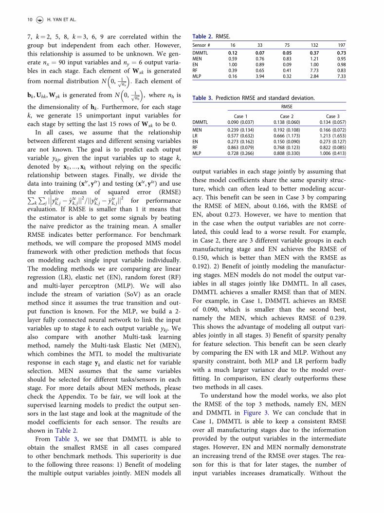
evaluation. If RMSE is smaller than 1 it means thatthe estimator is able to get some signals by beatingthe naive predictor as the training mean. A smallerRMSE indicates better performance. For benchmarkmethods, we will compare the proposed MMS modelframework with other prediction methods that focuson modeling each single input variable individually.The modeling methods we are comparing are linearregression (LR), elastic net (EN), random forest (RF)and multi-layer perceptron (MLP). We will alsoinclude the stream of variation (SoV) as an oraclemethod since it assumes the true transition and out-put function is known. For the MLP, we build a 2-layer fully connected neural network to link the inputvariables up to stage k to each output variable ykj. Wealso compare with another Multi-task learningmethod, namely the Multi-task Elastic Net (MEN),which combines the MTL to model the multivariateresponse in each stage yk and elastic net for variableselection. MEN assumes that the same variablesshould be selected for different tasks/sensors in eachstage. For more details about MEN methods, pleasecheck the Appendix. To be fair, we will look at thesupervised learning models to predict the output sen-sors in the last stage and look at the magnitude of themodel coefficients for each sensor. The results areshown in Table 2.

From Table 3, we see that DMMTL is able toobtain the smallest RMSE in all cases comparedto other benchmark methods. This superiority is dueto the following three reasons: 1) Benefit of modelingthe multiple output variables jointly. MEN models all

output variables in each stage jointly by assuming thatthese model coefficients share the same sparsity struc-ture, which can often lead to better modeling accur-acy. This benefit can be seen in Case 3 by comparingthe RMSE of MEN, about 0.166, with the RMSE ofEN, about 0.273. However, we have to mention thatin the case when the output variables are not corre-lated, this could lead to a worse result. For example,in Case 2, there are 3 different variable groups in eachmanufacturing stage and EN achieves the RMSE of0.150, which is better than MEN with the RMSE as0.192). 2) Benefit of jointly modeling the manufactur-ing stages. MEN models do not model the output var-iables in all stages jointly like DMMTL. In all cases,DMMTL achieves a smaller RMSE than that of MEN.For example, in Case 1, DMMTL achieves an RMSEof 0.090, which is smaller than the second best,namely the MEN, which achieves RMSE of 0.239.This shows the advantage of modeling all output vari-ables jointly in all stages. 3) Benefit of sparsity penaltyfor feature selection. This benefit can be seen clearlyby comparing the EN with LR and MLP. Without anysparsity constraint, both MLP and LR perform badlywith a much larger variance due to the model over-fitting. In comparison, EN clearly outperforms thesetwo methods in all cases.

To understand how the model works, we also plotthe RMSE of the top 3 methods, namely EN, MENand DMMTL in Figure 3. We can conclude that inCase 1, DMMTL is able to keep a consistent RMSEover all manufacturing stages due to the informationprovided by the output variables in the intermediatestages. However, EN and MEN normally demonstratean increasing trend of the RMSE over stages. The rea-son for this is that for later stages, the number ofinput variables increases dramatically. Without the

Table 2. RMSE.Sensor # 16 33 75 132 197

DMMTL 0.12 0.07 0.05 0.37 0.73MEN 0.59 0.76 0.83 1.21 0.95EN 1.00 0.89 0.09 1.00 0.98RF 0.39 0.65 0.41 7.73 0.83MLP 0.16 3.94 0.32 2.84 7.33

Table 3. Prediction RMSE and standard deviation.RMSE

Case 1 Case 2 Case 3DMMTL 0.090 (0.037) 0.138 (0.060) 0.134 (0.057)

MEN 0.239 (0.134) 0.192 (0.108) 0.166 (0.072)LR 0.577 (0.632) 0.666 (1.173) 1.213 (1.653)EN 0.273 (0.162) 0.150 (0.090) 0.273 (0.127)RF 0.863 (0.079) 0.768 (0.123) 0.822 (0.085)MLP 0.728 (0.266) 0.808 (0.330) 1.006 (0.413)

10 H. YAN ET AL.

guidance of the output variables in the intermediatestages, both EN and MEN cannot find the importantvariables easily. In Case 2, the RMSEs of all methodsincrease over the stages due to the decrease independency between the manufacturing stages.However, DMMTL still outperforms others. In Case 3,DMMTL has a slightly larger error compared to MENin the initial stages. The reason for this is that the firstthree stages in Case 3 are actually completely inde-pendent. However, DMMTL is forced to learn adependency between these stages, which could lead toa worse result. When the stages become dependentafter Stage 3 (e.g., stage 4 is related to stage 1, andstage 5 is related to stage 2), DMMTL is able toquickly exploit this dependency and outperform allother benchmark methods.

Furthermore, we would like to compare the inputvariable selection accuracy for Case 2 and Case 3 forthe last output variable in the last stage (Stage 9). It isworth noting that only the proposed method, EN andMEN, are able to perform the feature selection byselecting the non-zero elements of the model due tothe sparsity penalty. Other benchmark models, suchas LR, RF, and MLP cannot perform variable selectionnaively. Recall that the data are already normalized tomean 0 and variance 1. For LR, we will use the abso-lute value of the model coefficient directly for thevariable importance score. For MLP, we will use onlythe norm of the model coefficient of the first layer(connected to the input variables) as the input vari-able importance score. For RF, we propose to use thefeature importance metric computed by the averageaccuracy gain of each split according to each individ-ual variable. The result of the percentage of the inputvariable identification is shown in Table 4.

To evaluate the variable selection accuracy, we canview the input variable identification problem as theclassification problem and we also compute the preci-sion, recall, and AUC score in Table 4. Precision isdefined as the percentage of identified variables thatare actually important. Recall is defined as the

percentage of important variables that are actuallyidentified. AUC is defined as the area under thereceiver operating characteristic curve. The thresholdto determine the important input variable is set tomaintain the false positive rate as 5 percent. FromTable 4, we can conclude that DMMTL is able toaccurately identify the input variables compared toother benchmark methods in both Case 2 and 3 withthe highest precision, recall, and AUC score. MENperforms the second best, due to the ability to useinformation from multiple output sensors jointlywithin each stage. MEN is especially able to achieve amuch higher recall score than the other benchmarkmethods, showing the strength of a multi-task learn-ing framework. To better understand how eachmethod performs feature selection, we also plot thefeature importance score computed by each methodin Figure 4. From Figure 4, we can conclude thatDMMTL is able to use the least number of input vari-ables to achieve the best prediction power comparedto all other benchmark methods due to the grouplasso penalty.

6. Case study

In this case study, we apply DMMTL to model thediaper assembly process introduced in Section 1. Wedivide the whole converting process into five stagesand identify 484 process variables (e.g. temperature,pressure, etc.) as inputs and 200 quality measurements(e.g. product dimensions) as output variables in themodel. Due to the complex physical process involved,

Figure 3. RMSE according to each stage.

Table 4. Input variable identification accuracy.Precision Recall AUCCase 2 Case 3 Case 2 Case 3 Case 2 Case 3

DMMTL 0.795 0.867 0.515 0.871 0.810 0.958MEN 0.677 0.834 0.280 0.671 0.633 0.916LR 0.143 0.724 0.022 0.3511 0.486 0.689EN 0.189 0.752 0.031 0.404 0.465 0.706RF 0.167 0.589 0.027 0.191 0.463 0.599MLP 0.333 0.348 0.071 0.071 0.503 0.526

JOURNAL OF QUALITY TECHNOLOGY 11

it is very hard to derive the physics relationshipbetween the input variables and output variables. Thedetailed information of the number of input and out-put sensors in each stage is shown in Table 5. Due tothe privacy constraint, the name of the stages and thename of the sensors can not be given here.Furthermore, to increase the prediction power of ourmodel, we also use the output measurements from theprevious stage as input variables to the next stage.Because the manufacturing data is very noisy, we useboth the Huber loss function and the traditionalresidual sum of squares for comparison. We also com-pare DMMTL with several benchmark methods,including the multi-task elastic net (MEN), ridgeregression (RR), elastic net (EN), random forest (RF),and multi-layer perception (MLP). We do not includelinear regression (LR) in the comparison because itsparameter estimation is numerically unstable and itcan also be seen as a special case of RR without add-ing penalties.

One interesting phenomenon in the realistic casestudy is that not all output variables can be predictedwell based on the input variables. Given the complex-ity of the manufacturing process, even with 484 inputvariables some of the important characteristics of theunderlying process are still not measured by the sen-sors. Therefore, we try to find a model that canachieve excellent predictive power for most of the out-put variables. Furthermore, even knowing which out-put variables cannot be predicted is usefulinformation. This could guide adding more sensors orincreasing sample frequency. Finally, for more compli-cated cases, we used two-layer neural networks forboth emission and transition functions.

To compare how the methods are able to identifyrelated output variables, we first compute the RMSEof all 200 output variables. Recall that the RMSE isdefined as

Pk

Pj j ytek, j � ytek, jjj2=jjytek, j � �ytrk, jjj2��� and if

its value is smaller than 1 then that indicates the

model can achieve a better prediction than the naivepredictor based on the mean response value. Toevaluate the performance of different methods foridentifying the important variables, we first computethe 20 percent, 40 percent, 50 percent and 70 per-cent quantiles of the 200 RMSE scores in Table 6 for200 output variables for each method. We then choosethresholds on the RMSE ranging from 0.05 to 0.95and define the number of output variables with theRMSE score smaller than the threshold as the numberof identified related output variables. In Figure 5, weplot the number of identified related output variablesfor different thresholds.

Table 6 shows that DMMTL can achieve a lower RMSEover all quantiles 20 percent, 40 percent, 50 percent and70 percent. In particular, for the 20 percent quantile,DMMTL with Huber and mean square error lossfunction achieve the RMSE of 0.29 and 0.39, whichindicates the strong prediction power (i.e., muchsmaller than 1). Furthermore, when comparing themedian of the RMSE, only the proposed methods areable to achieve RMSE lower than 0.9. This can also beseen from Figure 5 that DMMTL outperforms allother benchmark methods due to the ability to com-bine the modeling with multiple output variables in

Figure 4. Identified important sensor for Case 2 and Case 3.

Table 5. Number of input and output variables foreach stage.

Stage 1 Stage 2 Stage 3 Stage 4 Stage 5

Input Variables 110 86 165 120 0Output Variables 20 64 10 90 16

Table 6. Quantiles of Prediction RMSE.Quantile 20% 40% 50% 70%

DMMTL (Huber) 0.29 0.73 0.87 1.01DMMTL (MSE) 0.39 0.71 0.81 0.99Multi-task Elastic Net 0.79 0.88 0.92 0.99Elastic Net 0.60 0.91 0.99 1.00Random Forest 0.53 0.79 0.93 1.11Multi-layer Perception 0.76 1.83 2.59 5.68

12 H. YAN ET AL.

different stages in a unified model. Furthermore, fromTable 6, we see that DMMTL with the Huber lossfunction is able to outperform the mean square errorloss function at the 20 percent and 40 percent quan-tiles or when the threshold is small as shown inFigure 5. The reason is that the Huber loss function ismore robust to outlier sensing variables and therefore,will focus more on reducing the loss functions of theoutput variables which are truly correlated to theinput variables. RF and EN’s performances followimmediately after our proposed method because theyhave the ability to select important variables. MLP, ingeneral, performs worse due to the lack of penaliza-tion and feature selection. MEN performs the worst inthis example since there are many uncorrelated output

Figure 5. Number of identified important output variableswith different threshold on the prediction RMSE.

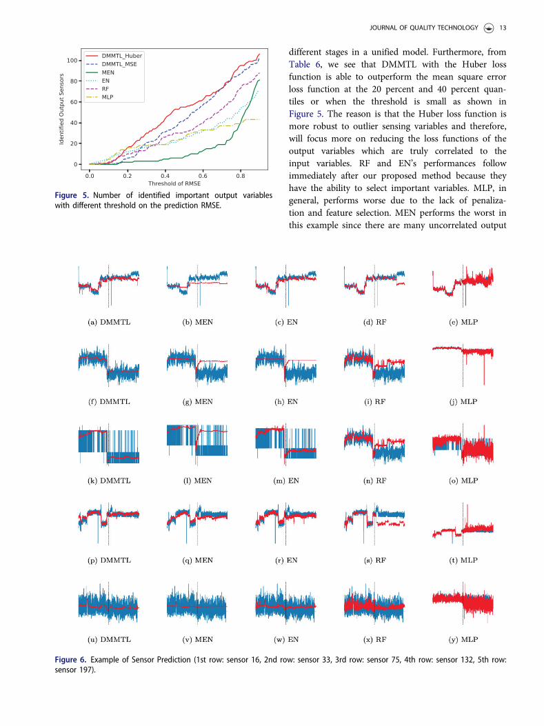
Figure 6. Example of Sensor Prediction (1st row: sensor 16, 2nd row: sensor 33, 3rd row: sensor 75, 4th row: sensor 132, 5th row:sensor 197).

JOURNAL OF QUALITY TECHNOLOGY 13

variables even in the same stage, which violates theassumption of MEN that the sparsity structure for allinput variables in the same stage is the same.

To demonstrate the performance of the predictionaccuracy for all methods, in Figure 6 we plot the pre-dicted signals and the true signal for the output varia-bles for both training and testing data. A dashed blackline is added in each plot to separate the training andtesting data. We select output sensors 16, 33, 75, 132,197 for demonstration in stage 1, 2, 3, 4, 5, respect-ively. The RMSE according to these output sensorsand the selected number of input variables of eachmethod are shown in Tables 3 and 7.

From Figure 6 and Table 7, we first conclude thatthese output variables share similar patterns. Forexample, Output 16 has a meanshift during time 1961and Output 33, 75, and 197 has a meanshift at time2813. Output 132 have meanshifts at both time points.DMMTL is able to achieve the least RMSE among allmethods due to its ability to combine all output sen-sors in a unified model, therefore leading to a bettermodel for all output sensors. EN also achieves goodperformance for Output 16 and 75. For Output 33

and 132, only DMMTL is able to accurately predictthe trend. RF sometimes does not capture the trendcorrectly. MLP typically overfits the data, and there-fore it normally produces much larger noises in thetesting data. MEN typically underfits the data due toits strong assumption that the models for output sen-sors in the same stage must share the same sparsitypatterns. In terms of the number of input sensorsidentified, typically EN is able to identify the leastnumber of input sensors, followed by DMMTL andMEN. MLP is not able to perform feature selection,which leads to severe over-fitting. In conclusion, wesee that DMMTL is able to achieve the least RMSEwith a relatively small number of selectedinput sensors.

Finally, in Figure 7, we also plot the top threeimportant input variables identified for all these fiveoutput variables. Among them, Input 744 can explainthe meanshift at time 2813 for all output variablesand Input 747 can explain some of the other smallmeanshifts for Output 16 and 33. Finally, Input 733and Input 67 are able to explain the small increasingtrend in Output 33 and 197, respectively. We havevalidated that the selected input variables indeed canexplain the variation for the selected output variablefrom the domain knowledge.

7. Conclusion

Modeling complex multistage manufacturing systemsis an important research topic for accurate process

Table 7. Number of input sensors identified.Sensor # 16 33 75 132 197

DMMTL 16 20 21 21 21MEN 35 35 35 35 36EN 18 18 18 16 16RF 21 116 151 30 342MLP 119 225 225 593 682

Figure 7. Top three important input variables identified by DMMTL for Output 16, 33, 75, 132 and 197.

14 H. YAN ET AL.

prediction, monitoring, diagnosis and control. Thispaper proposes a deep transition model with multi-task learning to jointly model all output sensing varia-bles with the input sensing variables according to thesequential production line structure. Furthermore,since the dimensionality of the input sensing variablesand output sensing variables can be very high, we sug-gest reducing the dimensionality by utilizing thesparse regularization and robust Huber loss functionto select the important sensing variables. DMMTL hasbeen tested through several simulated studies and arealistic case study of a real diaper manufacturing sys-tem. The results demonstrate that it achieves a betterprediction accuracy as well as a better local and globalinterpretability by identifying important relationshipbetween input and output sensing variables.

There are several future research directions that wewould like to investigate. One is to extend thismethod to heterogeneous measurements with morestage dependencies (e.g., tree structures) other thanthe production line set up in series. Another extensionis to study the proposed algorithm under the stochas-tic transition of the hidden variables similar to thestream of variation models.

Funding

This work is partially funded by the grants from NSF DMS1830363 and NSF CMMI 1922739. The support is gratefullyacknowledged.

About the authors

Hao Yan received his BS degree in Physics from the PekingUniversity, Beijing, China, in 2011. He also received a MSdegree in Statistics, a MS degree in Computational Scienceand Engineering, and a PhD degree in IndustrialEngineering from Georgia Institute of Technology, Atlanta,in 2015, 2016, 2017, respectively. Currently, he is anAssistant Professor in the School of Computing,Informatics, and Decision Systems Engineering at ASU. Hisresearch interests focus on developing scalable statisticallearning algorithms for large-scale high-dimensional datawith complex heterogeneous structures to extract usefulinformation for the purpose of system performance assess-ment, anomaly detection, intelligent sampling and decisionmaking. Dr. Yan was also the recipient of multiple awardsincluding best paper award in IEEE TASE, IISE Transactionand ASQ Brumbaugh Award. Dr. Yan is a member of IEEE,INFORMS and IIE.

Nurretin Dorukhan Sergin is a doctoral candidate at theIndustrial Engineer program at Arizona State University.His current research is focused on out-of-distributionbehaviors of deep neural networks and spatiotemporal mod-eling of urban mobility. During his master’s, he did research

on agent-based modeling and its application to computa-tional social simulation problems.

William A. Brenneman is a Research Fellow and theGlobal Statistics Discipline Leader at Procter & Gamble inthe Data and Modeling Sciences Department and anAdjunct Professor of Practice at Georgia Tech in theStewart School of Industrial and Systems Engineering. Sincejoining P&G, he has worked on a wide range of projectsthat deal with statistics applications in his areas of expertise:design and analysis of experiments, robust parameterdesign, reliability engineering, statistical process control,computer experiments, machine learning and statisticalthinking. He was also instrumental in the development ofan in-house statistics curriculum. He received a Ph.D. inStatistics from the University of Michigan, an MSin Mathematics from the University of Iowa and a BA inMathematics and Secondary Education from Tabor College.He is a Fellow in both the American Statistical Association(ASA) and the American Society for Quality (ASQ). He hasserved as ASQ Statistics Division Chair, ASA Quality andProductivity Section Chair and as Associate Editor forTechnometrics. William also has seven years of experienceas an educator at the high school and college level.

Stephen Joseph Lange is Managing Member of ProcessDev,LLC, a manufacturing process consultancy, and retired as aResearch Fellow from the Procter & Gamble Company,where he had a 35-year career in Research andDevelopment, developing processes and materials for newproducts and product improvements.

Shan Ba is a data science applied researcher at LinkedIn.He had previously worked as a group data scientist at theProcter & Gamble Company and an assistant professorof statistics at the Fariborz Maseeh Department ofMathematics and Statistics, Portland State University. Hereceived his Ph.D. in Industrial Engineering from GeorgiaInstitute of Technology.

ORCID

Hao Yan http://orcid.org/0000-0002-4322-7323

References

Abellan-Nebot, J. V., J. Liu, F. R. Subiron, and J. Shi. 2012.State space modeling of variation propagation in multi-station machining processes considering machining-induced variations. Journal of Manufacturing Science andEngineering 134 (2):021002. doi: 10.1115/1.4005790.

Apley, D. W., and J. Zhu. 2020. Visualizing the effects ofpredictor variables in black box supervised learningmodels. Journal of the Royal Statistical Society: Series B(Statistical Methodology) 82 (4):1059–1086.

Apley, D., and J. Shi. 1998. Diagnosis of multiple fixturefaults in panel assembly. Journal of ManufacturingScience and Engineering 120 (4):793–801. doi: 10.1115/1.2830222.

Bak Ir, B., _I. Batmaz, F. G€unt€urk€un, _I. _Ipekci, G. K€oksal,and N. €Ozdemirel. 2006. Defect cause modeling with

JOURNAL OF QUALITY TECHNOLOGY 15

decision tree and regression analysis. World Academy ofScience, Engineering and Technology 24:1–4.

Bottou, L. 2010. Large-scale machine learning with stochas-tic gradient descent. In Proceedings of COMPSTAT’2010,177–86. Heidelberg, Germany: Springer.

Caruana, R. 1997. Multitask learning. Machine Learning 28(1):41–75. doi: 10.1023/A:1007379606734.

Ceglarek, D., and J. Shi. 1996. Fixture failure diagnosis forautobody assembly using pattern recognition. Journal ofEngineering for Industry 118 (1):55–66. doi: 10.1115/1.2803648.

Chang, D. S., and S.-T. Jiang. 2002. Assessing quality per-formance based on the on-line sensor measurementsusing neural networks. Computers & IndustrialEngineering 42 (2–4):417–24. doi: 10.1016/S0360-8352(02)00035-9.

Correa, M., C. Bielza, M. d J. Ramirez, and J. R. Alique.2008. A Bayesian network model for surface roughnessprediction in the machining process. InternationalJournal of Systems Science 39 (12):1181–92. doi: 10.1080/00207720802344683.

Ding, Y., J. Jin, D. Ceglarek, and J. Shi. 2005. Process-ori-ented tolerancing for multi-station assembly systems. IIETransactions 37 (6):493–508. doi: 10.1080/07408170490507774.

Friedman, N., D. Geiger, and M. Goldszmidt. 1997.Bayesian network classifiers. Machine Learning 29 (2/3):131–63. doi: 10.1023/A:1007465528199.

Graves, A., and J. Schmidhuber. 2009. Offline handwritingrecognition with multidimensional recurrent neural net-works. In Advances in Neural Information ProcessingSystems, 545–52, Vancouver, Canada. San Francisco:Morgan Kau.

Graves, A., A-R Mohamed, and G. Hinton. 2013a. Speechrecognition with deep recurrent neural networks. In IEEEInternational Conference on Acoustics, Speech and SignalProcessing (ICASSP), 6645–6649. IEEE.

Graves, A., A.-R. Mohamed, and G. Hinton. 2013b. Speechrecognition with deep recurrent neural networks. 2013IEEE International Conference on Acoustics, Speech andSignal Processing, 6645–6649. IEEE.

Hao, L., L. Bian, N. Gebraeel, and J. Shi. 2017. Residual lifeprediction of multistage manufacturing processes withinteraction between tool wear and product quality deg-radation. IEEE Transactions on Automation Science andEngineering 14 (2):1211–24. doi: 10.1109/TASE.2015.2513208.

Huang, Q., S. Zhou, and J. Shi. 2002. Diagnosis of multi-operational machining processes through variation propa-gation analysis. Robotics and Computer-IntegratedManufacturing 18 (3–4):233–9. doi: 10.1016/S0736-5845(02)00014-5.

Jemwa, G. T., and C. Aldrich. 2005. Improving processoperations using support vector machines and decisiontrees. AIChE Journal 51 (2):526–43. doi: 10.1002/aic.10315.

Jensen, F. V. 1996. An introduction to Bayesian networks,Vol. 210. London: UCL press.

Jin, R., J. Li, and J. Shi. 2007. Quality prediction and controlin rolling processes using logistic regression. Transactionsof NAMRI/SME 35:113–20.

Jin, J., and J. Shi. 1999. State space modeling of sheet metalassembly for dimensional control. Journal ofManufacturing Science and Engineering 121 (4):756–62.doi: 10.1115/1.2833137.

Jin, R., and J. Shi. 2012. Reconfigured piecewise linearregression tree for multistage manufacturing process con-trol. IIE Transactions 44 (4):249–61. doi: 10.1080/0740817X.2011.564603.

Jin, M., and F. Tsung. 2009. A chart allocation strategy formultistage processes. IIE Transactions 41 (9):790–803.doi: 10.1080/07408170902789068.

Joe Qin, S. 2003. Statistical process monitoring: basics andbeyond. Journal of Chemometrics 17 (8–9):480–502. doi:10.1002/cem.800.

Kourti, T., J. Lee, and J. F. Macgregor. 1996. Experienceswith industrial applications of projection methods formultivariate statistical process control. Computers &Chemical Engineering 20:S745–S750. doi: 10.1016/0098-1354(96)00132-9.

Kuhn, M., and K. Johnson. 2013. Applied predictive model-ing, Vol. 26. New York: Springer.

Lawless, J., R. Mackay, and J. Robinson. 1999. Analysis ofvariation transmission in manufacturing processes–part I.Journal of Quality Technology 31 (2):131–42. doi: 10.1080/00224065.1999.11979910.

LeCun, Y., B. E. Boser, J. S. Denker, D. Henderson, R. E.Howard, W. E. Hubbard, and L. D. Jackel. 1990.Handwritten digit recognition with a back-propagationnetwork. In Advances in Neural Information ProcessingSystems, 396–404, Denver, CO. San Francisco, CA:Morgan Kaufmann.

Li, Y., and F. Tsung. 2009. False discovery rate-adjustedcharting schemes for multistage process monitoring andfault identification. Technometrics 51 (2):186–205. doi: 10.1198/TECH.2009.0019.

Liu, K., and J. Shi. 2013. Objective-oriented optimal sensorallocation strategy for process monitoring and diagnosisby multivariate analysis in a Bayesian network. IIETransactions 45 (6):630–43. doi: 10.1080/0740817X.2012.725505.

Liu, J., J. Shi, and S. J. Hu. 2009. Quality-assured setupplanning based on the stream-of-variation model formulti-stage machining processes. IIE Transactions 41 (4):323–34. doi: 10.1080/07408170802108526.

Liu, K., X. Zhang, and J. Shi. 2014. Adaptive sensor alloca-tion strategy for process monitoring and diagnosis in abayesian network. IEEE Transactions on AutomationScience and Engineering 11 (2):452–62. doi: 10.1109/TASE.2013.2287101.

Lowry, C. A., and D. C. Montgomery. 1995. A review ofmultivariate control charts. IIE Transactions 27 (6):800–10. doi: 10.1080/07408179508936797.

MacGregor, J. F., and T. Kourti. 1995. Statistical processcontrol of multivariate processes. Control EngineeringPractice 3 (3):403–14. doi: 10.1016/0967-0661(95)00014-L.

Mateos, G., and G. B. Giannakis. 2012. Robust nonparamet-ric regression via sparsity control with application to loadcurve data cleansing. IEEE Transactions on SignalProcessing 60 (4):1571–84. doi: 10.1109/TSP.2011.2181837.

Molnar, C. 2020. Interpretable Machine Learning. Morrisville,NC: Lulu Press.

16 H. YAN ET AL.

Obozinski, G., B. Taskar, and M. Jordan. 2006. Multi-taskfeature selection. Technical report, Department ofStatistics, University of California, Berkeley.

Paynabar, K., J. Jin, and M. Pacella. 2013. Monitoring anddiagnosis of multichannel nonlinear profile variationsusing uncorrelated multilinear principal component ana-lysis. IIE Transactions 45 (11):1235–47. doi: 10.1080/0740817X.2013.770187.

Reckhow, K. H. 1999. Water quality prediction and prob-ability network models. Canadian Journal of Fisheries andAquatic Sciences 56 (7):1150–8. doi: 10.1139/f99-040.

Shewhart, W. A. 1931. Economic control of quality of manu-factured product. ASQ Quality Press.

Shi, J. 2006. Stream of variation modeling and analysis formultistage manufacturing processes. Boca Raton, FL: CRCPress.

Shiu, B., D. Ceglarek, and J. Shi. 1997. Flexible beam-basedmodeling of sheet metal assembly for dimensional con-trol. In Transactions-North American ManufacturingResearch Institution of SME, 24, 49–54.

Skinner, K. R., D. C. Montgomery, G. C. Runger, J. W.Fowler, D. R. McCarville, T. R. Rhoads, and J. D. Stanley.2002. Multivariate statistical methods for modeling andanalysis of wafer probe test data. IEEE Transactions onSemiconductor Manufacturing 15 (4):523–30. doi: 10.1109/TSM.2002.804901.

Tam, C., T. K. Tong, T. C. Lau, and K. Chan. 2004.Diagnosis of prestressed concrete pile defects using prob-abilistic neural networks. Engineering Structures 26 (8):1155–62. doi: 10.1016/j.engstruct.2004.03.018.

Woodall, W. H. 2007. Current research on profile monitor-ing. Production 17 (3):420–5. doi: 10.1590/S0103-65132007000300002.

Yan, H., K. Paynabar, and M. Pacella. 2019. Structuredpoint cloud data analysis via regularized tensor regressionfor process modeling and optimization. Technometrics 61(3):385–395.

Yan, H., K. Paynabar, and J. Shi. 2015. Image-based processmonitoring using low-rank tensor decomposition. IEEETransactions on Automation Science and Engineering 12(1):216–27. doi: 10.1109/TASE.2014.2327029.

Yan, H., K. Paynabar, and J. Shi. 2017. Anomaly detectionin images with smooth background via smooth-sparsedecomposition. Technometrics 59 (1):102–14. doi: 10.1080/00401706.2015.1102764.

Yu, J., and M. M. Rashid. 2013. A novel dynamic bayesiannetwork-based networked process monitoring approachfor fault detection, propagation identification, and rootcause diagnosis. AIChE Journal 59 (7):2348–65. doi: 10.1002/aic.14013.

Yuan, M., and Y. Lin. 2006. Model selection and estimationin regression with grouped variables. Journal of the RoyalStatistical Society: Series B (Statistical Methodology) 68(1):49–67. doi: 10.1111/j.1467-9868.2005.00532.x.

Zhang, C., H. Yan, S. Lee, and J. Shi. 2020. Dynamic multi-variate functional data modeling via sparse subspacelearning. Technometrics, in press.

Zhou, S., Y. Chen, and J. Shi. 2004. Statistical estimationand testing for variation root-cause identification ofmultistage manufacturing processes. IEEE Transactionson Automation Science and Engineering 1 (1):73–83. doi:10.1109/TASE.2004.829427.

Zhou, S., Q. Huang, and J. Shi. 2003. State space modelingof dimensional variation propagation in multistagemachining process using differential motion vectors. IEEETransactions on Robotics and Automation 19 (2):296–309.

Zhou, Q., Z. Xiong, J. Zhang, and Y. Xu. 2006. Hierarchicalneural network based product quality prediction ofindustrial ethylene pyrolysis process. In InternationalSymposium on Neural Networks, 1132–1137. Springer.

Appendix

A. Relationship to stream of variation

The foundation of SoV methodology is a mathematical modelthat links the output variables (e.g., key quality characteristicsof the product) with key input variables (e.g., key processsensing variables) through the state space representation.

hk ¼ Wxkxk þ Uhkhk�1 þ ehk, yk ¼ Vykhk þ eyk (11)

The variable hk is the state vector representing the out-put variables at stage k. ehk and eyk are the modeling errorand measurement error, respectively. The coefficient matri-ces Wxk,Uhk, and Vyk are determined by product and pro-cess design information at stage k. Wxk represents theimpact of the new stage process to the product. Uhk repre-sents the transition from stage k� 1 to stage k. Vyk is themeasurement matrix, which links the hidden state hk andthe output yk:

These mathematical models have achieved great successin MMS modeling by integrating the product and processdesign information and modeling the variation propagationin the MMS. However, the SoV methodology assumes thatthe key output variables yk and key input variables xk havebeen correctly identified. Furthermore, it requires the matri-ces Wxk,Uhk, and Vyk are known in each stage k, which isnot possible if the system is too complex. Finally, it assumesthe linear transition matrix between states which could bean over-simplification in many real cases. However, SoVassumes that the transition between the state variables areknown as the linear stochastic function. The proposedDMMTL assumes that the transition is unknown nonlinearfunctions. Extending the framework to stochastic functionswould be one of our future work.

B. Relationship to recurrent neural network

The formulation of RNN methodology is a neural networkthat links the output variables yk, input variables xk in aneural network. More specifically, at each time k, the outputyk and input xk are linked together via the hidden state hkin (Equation (12)).

hk ¼ rðWxxk þ Uhhk�1 þ bhÞ, yk ¼ Vyhk þ by (12)

In RNN, it is typically assumed that the system is time-invariant, which means the model parameters Wx,Ux,Vy

are independent of k. RNN has achieved great success inmachine translation problems (Graves, Mohamed, andHinton 2013a), handwriting recognition (Graves andSchmidhuber 2009) and speech recognition (Graves,Mohamed, and Hinton 2013b). Furthermore, model param-eters Wx,Ux,Vy can be learned in an end-to-end fashion

JOURNAL OF QUALITY TECHNOLOGY 17

via the combination of back-propagation (LeCun et al.1990) and stochastic gradient descent (Bottou 2010).

However, the major limitation of using RNN in MMS isthat different manufacturing stages are inherently different.The underlying physics is entirely different for each stagewhich not only results in the different transition matrixWx,Uh, and Vy: RNN also assumes the same set of varia-bles are predicted in each time. However, in MMS, differentquality inspection sensors are set up in each manufacturingstage. Finally, RNN is a complicated model and can notachieve input and output variable selection as the pro-posed approach.

C. Proof of Proposition 2

Proof. Considering the loss function

minakjXk, j

jjykj � gkjðhk;HÞ � akjjj2 þ kxXnx, ki¼1

jjwi, xkjj2

þ k2jjHjj2 þ c

Xk, j

jjakjjj1 (13)

Here, the loss function in (13) can be decoupled intoeach pair of (k, j) individually. Therefore, each akj can besolved individually by optimizing

jjykj � gkjðhk;HÞ � akjjj2 þ cjjakjjj1and can be solved by

akj ¼ Sc=2ðykj � gkjðhk;HÞÞ,To optimize the wi, xk, we will follow the derivation of

the proximal gradient algorithm the Taylor expansion ofLðH,AÞ asLðH,AÞ � LðHðt�1Þ,AÞ

þXi

@LðHðt�1Þ,AÞ@wi, xk

wi, xk � wðt�1Þi, xk

� �þ L

2jjwi, xk

� wðt�1Þi, xk jj2

(14)

L is the Lipschitz constance of LðH,AÞ: Therefore, weaim to minimize the upper bound of LðH,AÞ þRðH,AÞas follows:

minfwi, xkgLðHðt�1Þ,AÞ þXi, k

@LðHðt�1Þ,AÞ@wi, xk

wi, xk � wðt�1Þi, xk

� �

þ L2

Xi, k

jjwi, xk � wðt�1Þi, xk jj2 þ kx

Xi, k

jjwi, xkjj2 þk2

Xi, k

jjwi, xkjj2

Here, we find that the optimization can be decoupled toeach individual (i, k) as

minwi, xk

jjwi, xk � LLþ k

ðwðt�1Þi, xk � 1

L@LðHðt�1Þ,AÞ

@wi, xkÞjj2

þ 2kxLþ k

Xnx, ki¼1

jjwi, xkjj2,

and can be solved in closed form as

wðtÞi, xk ¼ S kx

Lþkð LLþ k

ðwðt�1Þi, xk � 1

L@LðHðt�1Þ,AÞ

@wi, xkÞÞ:

D. Back-propagation along the sequential stagesover parameters hk

We will discuss how to efficiently optimize the modelparameters H via stochastic gradient descent. Suppose wedenote Xn,Yn as the nth sample of the entire dataset withn ¼ 1, :::,Nn, then the loss function can be decomposed as

LðH; fXg, fYgÞ ¼ 1Nn

XNn

n¼1

XKk¼1

XNy, k

j¼1

logPðynkjjhk;HÞ: (15)

If the number of samples Nn is large, averaging the gra-dient over the entire dataset is normally slow. To addressthis, we propose to apply the mini-batch stochastic gradientalgorithm, which is widely used to optimize large-scalemachine learning problems. In each iteration t, we canchoose a subset of samples N t 2 f1, :::,Nng, where the gra-dient is only evaluated as the average of the subset of theentire samples in (16):

Hðtþ1Þ ¼ HðtÞ � 1jN tj

Xn2N t

@~LðXn,Yn;HðtÞÞ@H

: (16)

Now we will discuss how to compute the gradientaccording to the model coefficients H: H ¼ fh1, :::hKg:First, the likelihood can be decomposed into different sam-ples, stages, and output variables due to the conditionaldependency of the hidden variables hk0 in (17).

@

@hkLðx, y;HÞ ¼

XNn

n¼1

XKk0¼1

Xny, k0

j¼1

@

@hklogPðynk0 jjhk0 ; hgkÞ (17)

Therefore, we need to compute @@hk

logPðynk0 jjhk0 ; hgkÞ: Fork0 < k, it is obvious that

@@hk

logPðynk0 jjhk0 ; hgkÞ ¼ 0: However, if k0 k, we can

compute the gradient@ log Pðyn

k0 jjhk0 ;hgkÞ

@hkrecursively as

@ log Pðynk0 jjhk0 ;h

gkÞ

@hk¼ @ log Pðyn

k0 jjhk0 ;hgkÞ

@hk0@hk0@hk0�1

� � � @hkþ1@hk

@hk@hk

: By plugging

in this into (17), we can derive the gradient according tothe state transition parameters (18).

@

@hhkLðx, y;HÞ ¼

XKk0¼k

Xny, k0

j¼1

@ log Pðynk0jjhk0 ; hgkÞ@hk0

@hk0

@hk0�1� � � @hkþ1

@hk

@hk@hhk

:

(18)

Finally, to derive the gradient according to output coeffi-cient hgk, we can derive

@

@hgk

Lðx, y;HÞ ¼Xny, kj¼1

@ logPðynkjjhk; hgkÞ@h

gk

: (19)

We would then discuss how to compute the gradient

based for@ log Pðykjjhk;hgkÞ

@hk,

@ log Pðykjjhk;hgkÞ@h

gk

, @hk@hhk

, @hk@hk�1

: The com-

putation is shown as follows:

18 H. YAN ET AL.

Emission layer

@ log Pðykjjhk; hgkÞ@hk

¼ 2ðgkjðhk; hgkÞ � ykÞ@gkjðhk; hgkÞ

@hk@ log Pðykjjhk; hgkÞ

@hgk

¼ 2ðgkjðhk; hgkÞ � ykÞ@gkjðhk; hgkÞ

@hgk

Transition layer

@hk@hk�1

¼ @fkðhk�1, xk; hhkÞ

@hk�1,@hk@hhk

¼ @fkðhk�1, xk; hhkÞ

@hhk,@hk@xk

¼ @fkðhk�1, xk; hhkÞ

@xk

Depending on the different function forms of fkð�Þ andgkð�Þ, the gradient can be computed.

E. Multi-task elastic net

In this section, we will briefly review the multi-task elasticnet methods in the literature. Here, Y 2 R

n�k is the

multivariate output, where n is the number of the samplesand k is the number of tasks. X 2 R

n�p is the input varia-bles and p is the number of feature variables. W 2 R

p�k isthe regression coefficient matrix.

Finally, to impose the similarity between multiple tasks,the following regularization is used as follows.

12n

jjY � XWjj2 þ abjjWjj2, 1 þ12að1� bÞjjWjj2:

Here, jjWjj2, 1 ¼P

i

ffiffiffiffiffiffiffiffiffiffiffiffiffiffiPj W

2ij

qis the sum of norm of

each row of W, where jjWjj2, 1 encourages the samesparsity patterns among all tasks. For example, it is easyto show that when the number of tasks equals to one,the problem MEN reduces to the L1-norm regularizedoptimization problem (or Lasso). When there are mul-tiple tasks, the weights corresponding to the i-th featureare grouped together via the L2-norm of W.Furthermore, jjWjj2 is used to further regularize themodel to avoid the multicollinearity of the task inputmatrix X. a and b are two tuning parameters control thelevel of regularization.

JOURNAL OF QUALITY TECHNOLOGY 19