Deep Lesion Graphs in the Wild: Relationship Learning and Organization ofSignificant Radiology Image Findings in a Diverse Large-scale Lesion Database

Ke Yan, Xiaosong Wang, Le Lu, Ling Zhang, Adam P. HarrisonMohammadhadi Bagheri, Ronald M. Summers

Imaging Biomarkers and Computer-Aided Diagnosis Laboratory,Clinical Image Processing Services, Radiology and Imaging Sciences

National Institutes of Health Clinical Center, 10 Center Drive, Bethesda, MD 20892 {ke.yan, xiaosong.wang, ling.zhang3, mohammad.bagheri, rms}@nih.gov,

{lel, aharrison}@nvidia.com

Abstract

Radiologists in their daily work routinely find and an-notate significant abnormalities on a large number of ra-diology images. Such abnormalities, or lesions, have col-lected over years and stored in hospitals’ picture archivingand communication systems. However, they are basicallyunsorted and lack semantic annotations like type and loca-tion. In this paper, we aim to organize and explore them bylearning a deep feature representation for each lesion. Alarge-scale and comprehensive dataset, DeepLesion, is in-troduced for this task. DeepLesion contains bounding boxesand size measurements of over 32K lesions. To model theirsimilarity relationship, we leverage multiple supervision in-formation including types, self-supervised location coordi-nates, and sizes. They require little manual annotation effortbut describe useful attributes of the lesions. Then, a tripletnetwork is utilized to learn lesion embeddings with a se-quential sampling strategy to depict their hierarchical sim-ilarity structure. Experiments show promising qualitativeand quantitative results on lesion retrieval, clustering, andclassification. The learned embeddings can be further em-ployed to build a lesion graph for various clinically usefulapplications. An algorithm for intra-patient lesion matchingis proposed and validated with experiments.

1. Introduction

Large-scale datasets with diverse images and dense an-notations [9, 12, 22] play an important role in computer vi-sion and image understanding, but often come at the cost ofvast amounts of labeling. In computer vision, this cost hasspurred efforts to exploit weak labels [48, 19, 5], e.g., theenormous amount of weak labels generated everyday on theweb. A similar situation exists in the medical imaging do-main, except that annotations are even more time consum-

ing and require extensive clinical training, which precludesapproaches like crowd-sourcing. Fortunately, like web datain computer vision, a vast, loosely-labeled, and largely un-tapped data source does exist in the form of hospital pic-ture archiving and communication systems (PACS). Thesearchives house patient images and accompanying radiologi-cal reports, markings, and measurements performed duringclinical duties. However, data is typically unsorted, unorga-nized, and unusable in standard supervised machine learn-ing approaches. Developing means to fully exploit PACSradiology database becomes a major goal within the field ofmedical imaging.

This work contributes to this goal of developing an ap-proach to usefully mine, organize, and learn the relation-ships between lesions found within computed tomography(CT) images in PACS. Lesion detection, characterization,and retrieval is an important task in radiology [46, 11, 23,21]. The latest methods based on deep learning and con-volutional neural networks (CNNs) have achieved signifi-cantly better results than conventional hand-crafted imagefeatures [15, 23]. However, large amounts of training datawith high quality labels are often needed. To address thischallenge, we develop a system designed to exploit the rou-tine markings and measurements of significant findings thatradiologists frequently perform [10]. These archived mea-surements are potentially highly useful sources of data forcomputer-aided medical image analysis systems. However,they are basically unsorted and lack semantic labels, e.g.,lung nodule, mediastinal lymph node.

We take a feature embedding and similarity graph ap-proach to address this problem. First, we present a newdataset: DeepLesion, which was collected from the PACSof a major medical institute. It contains 32,120 axial CTslices from 10,594 CT imaging studies of 4,427 unique pa-tients. There are 1–3 lesions in each image with accompa-nying bounding boxes and size measurements. The lesionsare diverse but unorganized. Our goal is to understand them

1

and discover their relationships. In other words, can we or-ganize them so that we are able to (1) know their type andlocation; (2) find similar lesions in different patients, i.e.,content-based lesion retrieval; and (3) find similar lesions inthe same patient, i.e., lesion instance matching for diseasetracking?

As Fig. 1 illustrates, the above problems can be addressedby learning feature representations for each lesion that keepsa proper similarity relationship, i.e., lesions with similar at-tributes should have similar embeddings. To reduce anno-tation workload and leverage the intrinsic structure withinCT volumes, we use three weak cues to describe each le-sion: type, location, and size. Lesion types are obtained bypropagating the labels of a small amount of seed samples tothe entire dataset, producing pseudo-labels. The 3D relativebody location is obtained from a self-supervised body-partregression algorithm. Size is directly obtained by the radio-logical marking. We then define the similarity relationshipbetween lesions based on a hierarchical combination of thecues. A triplet network with a sequential sampling strategyis utilized to learn the embeddings. We also apply a multi-scale multi-crop architecture to exploit both context and de-tail of the lesions, as well as an iterative refinement strategyto refine the noisy lesion-type pseudo-labels.

Qualitative and quantitative experimental results demon-strate the efficacy of our framework for several highly im-portant applications. 1), we show excellent performance oncontent-based lesion retrieval [28, 47, 41, 21]. Effective so-lutions to this problem can help identify similar case his-tories, better understand rare disorders, and ultimately im-prove patient care [23]. We show that our embeddings canbe used to find lesions similar in type, location, and size.Most importantly, the embeddings can match lesions withsemantically similar body structures that are not specifiedin the training labels. 2), the embeddings are also success-fully applied in intra-patient lesion matching. Patients undertherapy typically undergo CT examinations (studies) at in-tervals to assess the effect of treatments. Comparing lesionsin follow-up studies with their corresponding ones in previ-ous studies constitutes a major part of a radiologist’s work-load [25]. We provide an automated tool for lesion match-ing which can significantly save time, especially for patientswith multiple follow-up studies [31].

2. Related work

Deep Metric Learning: Metric learning can be benefi-cial whenever we want to keep certain similarity relationshipbetween samples [2]. The siamese network [3] is a seminalwork in deep metric learning, which minimizes the distancebetween a pair of samples with the same label and pushessamples with different labels apart. It was improved by thetriplet network [29], which considers relative distances. Thetriplet network requires three samples to compute a loss: an

anchor A, a positive sample P with the same label as A,and a negative sample N with a different label. The net-work learns embeddings that respect the following distancerelationship:

‖f(A)− f(P )‖22 + m < ‖f(A)− f(N)‖22, (1)

where f is the embedding function to be learned and m isa predefined margin. Various improvements to the standardtriplet network have been proposed [49, 36, 4, 38, 37]. Threekey aspects in these methods are: how to define similaritybetween images, how to sample images for comparison, andhow to compute the loss function. Zhang et al. [49] gen-eralized the sampling strategy and triplet loss for multiplelabels with hierarchical structures or shared attributes. Sonet al. [37] employed label hierarchy to learn object embed-dings for tracking, where object class is a high-level labeland detection timestamp is low-level. Our sequential sam-pling strategy shares the similar spirit with them, but we lackwell-defined supervision cues in the dataset, so we proposedstrategies to leverage weak cues, e.g. self-supervised body-part regressor and iterative refinement.

Lesion Management: Great efforts have been devoted tolesion detection [40, 46], classification [6, 11], and retrieval[28, 47, 41, 21]. Recently, CNNs have become the methodof choice over handcrafted features due to the former’s su-perior performance [33, 39, 15, 23]. Our work is in line withcontent-based medical image retrieval, which has been sur-veyed in detail by [21]. Existing methods generally focus onone type of lesion (e.g. lung lesion or mammographic mass)and learn the similarity relationship based on manually an-notated labels [47, 41] or radiology reports [28]. To the bestof our knowledge, no work has been done on learning deeplesion embeddings on a large comprehensive dataset withweak cues. Taking a different approach, [16, 44] cluster im-ages or lesions to discover concepts in unlabeled large-scaledatasets. However, they did not leverage multiple cues toexplicitly model the semantic relationship between lesions.Several existing works on intra-patient lesion matching fo-cus on detecting follow-up lesions and matching them pixelby pixel [17, 26, 34, 43], which generally requires organsegmentation or time-consuming nonrigid volumetric regis-tration. Besides, they are designed for certain types of le-sions, whereas our lesion embedding can be used to matchall kinds of lesions.

3. DeepLesion DatasetDeepLesion dataset consists of over 32K clinically sig-

nificant findings mined from a major institute’s PACS. Tothe best of our knowledge, this dataset is the first to automat-ically extract lesions from challenging PACS sources. Im-portantly, the workflow described here can be readily scaledup and applied to multiple institutional PACS, providing ameans for truly massive scales of data.

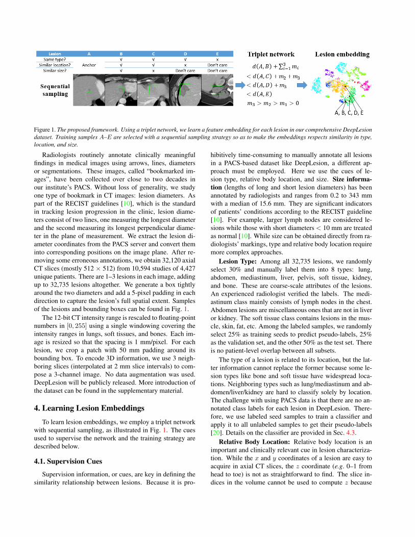
Figure 1. The proposed framework. Using a triplet network, we learn a feature embedding for each lesion in our comprehensive DeepLesiondataset. Training samples A–E are selected with a sequential sampling strategy so as to make the embeddings respects similarity in type,location, and size.

Radiologists routinely annotate clinically meaningfulfindings in medical images using arrows, lines, diametersor segmentations. These images, called “bookmarked im-ages”, have been collected over close to two decades inour institute’s PACS. Without loss of generality, we studyone type of bookmark in CT images: lesion diameters. Aspart of the RECIST guidelines [10], which is the standardin tracking lesion progression in the clinic, lesion diame-ters consist of two lines, one measuring the longest diameterand the second measuring its longest perpendicular diame-ter in the plane of measurement. We extract the lesion di-ameter coordinates from the PACS server and convert theminto corresponding positions on the image plane. After re-moving some erroneous annotations, we obtain 32,120 axialCT slices (mostly 512 × 512) from 10,594 studies of 4,427unique patients. There are 1–3 lesions in each image, addingup to 32,735 lesions altogether. We generate a box tightlyaround the two diameters and add a 5-pixel padding in eachdirection to capture the lesion’s full spatial extent. Samplesof the lesions and bounding boxes can be found in Fig. 1.

The 12-bit CT intensity range is rescaled to floating-pointnumbers in [0, 255] using a single windowing covering theintensity ranges in lungs, soft tissues, and bones. Each im-age is resized so that the spacing is 1 mm/pixel. For eachlesion, we crop a patch with 50 mm padding around itsbounding box. To encode 3D information, we use 3 neigh-boring slices (interpolated at 2 mm slice intervals) to com-pose a 3-channel image. No data augmentation was used.DeepLesion will be publicly released. More introduction ofthe dataset can be found in the supplementary material.

4. Learning Lesion Embeddings

To learn lesion embeddings, we employ a triplet networkwith sequential sampling, as illustrated in Fig. 1. The cuesused to supervise the network and the training strategy aredescribed below.

4.1. Supervision Cues

Supervision information, or cues, are key in defining thesimilarity relationship between lesions. Because it is pro-

hibitively time-consuming to manually annotate all lesionsin a PACS-based dataset like DeepLesion, a different ap-proach must be employed. Here we use the cues of le-sion type, relative body location, and size. Size informa-tion (lengths of long and short lesion diameters) has beenannotated by radiologists and ranges from 0.2 to 343 mmwith a median of 15.6 mm. They are significant indicatorsof patients’ conditions according to the RECIST guideline[10]. For example, larger lymph nodes are considered le-sions while those with short diameters < 10 mm are treatedas normal [10]. While size can be obtained directly from ra-diologists’ markings, type and relative body location requiremore complex approaches.

Lesion Type: Among all 32,735 lesions, we randomlyselect 30% and manually label them into 8 types: lung,abdomen, mediastinum, liver, pelvis, soft tissue, kidney,and bone. These are coarse-scale attributes of the lesions.An experienced radiologist verified the labels. The medi-astinum class mainly consists of lymph nodes in the chest.Abdomen lesions are miscellaneous ones that are not in liveror kidney. The soft tissue class contains lesions in the mus-cle, skin, fat, etc. Among the labeled samples, we randomlyselect 25% as training seeds to predict pseudo-labels, 25%as the validation set, and the other 50% as the test set. Thereis no patient-level overlap between all subsets.

The type of a lesion is related to its location, but the lat-ter information cannot replace the former because some le-sion types like bone and soft tissue have widespread loca-tions. Neighboring types such as lung/mediastinum and ab-domen/liver/kidney are hard to classify solely by location.The challenge with using PACS data is that there are no an-notated class labels for each lesion in DeepLesion. There-fore, we use labeled seed samples to train a classifier andapply it to all unlabeled samples to get their pseudo-labels[20]. Details on the classifier are provided in Sec. 4.3.

Relative Body Location: Relative body location is animportant and clinically relevant cue in lesion characteriza-tion. While the x and y coordinates of a lesion are easy toacquire in axial CT slices, the z coordinate (e.g. 0–1 fromhead to toe) is not as straightforward to find. The slice in-dices in the volume cannot be used to compute z because

CT volumes often have different scan ranges (start, end), notto mention variabilities in body lengths and organ layouts.For this reason, we use the self-supervised body part regres-sor (SSBR), which provides a relative z coordinate based oncontext appearance.

SSBR operates on the intuition that volumetric medicalimages are intrinsically structured, where the position andappearance of organs are relatively aligned. The superior-inferior slice order can be leveraged to learn an appearance-based z. SSBR randomly picks m equidistant slices from avolume, denoted j, j + k, . . . , j + k(m− 1), where j and kare randomly determined. They are passed through a CNNto get a score s for each slice, which is optimized using thefollowing loss function:

LSSBR = Lorder + Ldist;

Lorder = −∑m−2

i=0log h

(sj+k(i+1) − sj+ki

);

Ldist =∑m−3

i=0g(∆i+1 −∆i),

∆i = sj+k(i+1) − sj+ki,

(2)

where h is the sigmoid function, g is the smooth L1 loss[14]. Lorder requires slices with larger indices to have largerscores. Ldist makes the difference between two slice scoresproportional to their physical distance. The order loss anddistance loss terms collaborate to push each slice score to-wards the correct direction relative to other slices. Afterconvergence, slices scores are normalized to [0, 1] to obtainthe z coordinates without having to know which score cor-responds to which body part. The framework of SSBR isshown in Fig. 2.

Figure 2. Framework of the self-supervised body part regressor(SSBR).

In DeepLesion, some CT volumes are zoomed in on aportion of the body, e.g. only the left half is shown. Tohandle them, we train SSBR on random crops of the axialslices. Besides, SSBR does not perform well on body partsthat are rare in the training set, e.g. head and legs. There-fore, we train SSBR on all data first to detect hard volumesby examining the correlation coefficient (r) between sliceindices and slice scores, where lower r often indicates rare

body parts in the volume. Then, SSBR is trained again on aresampled training set with hard volumes oversampled.

4.2. Sequential Sampling

Similar to [49, 37], we leverage multiple cues to describethe relationship between samples. A naıve strategy wouldbe to treat all cues equally, where similarity can be calcu-lated by, for instance, averaging the similarity of each cue.Another strategy assumes a hierarchical structure exists inthe cues. Some high-level cues should be given higher pri-ority. This strategy applies to our task, because intuitivelylesions of the same type should be clustered together first.Within each type, we hope lesions that are closer in locationto be closer in the feature space. If two lesions are similar inboth type and location, they can be further ranked by size.This is a conditional ranking scheme.

To this end, we adopt a sequential sampling strategy toselect a sequence of lesions following the hierarchical re-lationship above. As depicted in Fig. 1, an anchor lesionA is randomly chosen first. Then, we look for lesions withsimilar type, location, and size with A and randomly pickB from the candidates. Likewise, C is a lesion with similartype and location but dissimilar size; D is similar in type butdissimilar in location (its size is not considered); E has a dif-ferent type (its location and size are not considered). Here,two lesions are similar in type if they have the same pseudo-label; they are similar in location (size) if the Euclidean dis-tance between their location (size) vectors is smaller than athreshold Tlow, whereas they are dissimilar if the distance islarger than Thigh. We do not use hard triplet mining as in[29, 27] because of the noisy cues. Fig. 3 presents some ex-amples of lesion sequences. Note that there is label noise inthe fourth row, where lesion D does not have the same typewith A – C (soft tissue versus pelvis).

A selected sequence can be decomposed into threetriplets: ABC, ACD and ADE. However, they are notequal, because we hope two lesions with dissimilar typesto be farther apart than two with dissimilar locations, fol-lowed by size. Hence, we apply larger margins to higher-level triplets [49, 4]. Our loss function is defined as:

L =1

2S

S∑i=1

[max(0, d2AB − d2AC + m1) (3)

+ max(0, d2AC − d2AD + m2)

+ max(0, d2AD − d2AE + m3)].

m3 > m2 > m1 > 0 are the hierarchical margins; Sis the number of sequences in each mini-batch; dij is theEuclidean distance between two samples in the embeddingspace. The idea in sequential sampling resembles that ofSSBR (Eq. 2): ranking a series of samples to make themself-organize and move to the right place in the featurespace.

Figure 3. Sample training sequences. Each row is a sequence.Columns 1–5 are examples of lesions A–E in Fig. 1, respectively.

Figure 4. Network architecture of the proposed triplet network.

4.3. Network Architecture and Training Strategy

VGG-16 [35] is adopted as the backbone of the tripletnetwork. As illustrated in Fig. 4, we input the 50mm-paddedlesion patch, then combine feature maps from 4 stages ofVGG-16 to get a multi-scale feature representation with dif-ferent padding sizes [13, 18]. Because of the variable sizesof the lesions, region of interest (ROI) pooling layers [14]are used to pool the feature maps to 5× 5× num channelseparately. For conv2 2, conv3 3, and conv4 3, the ROI isthe bounding box of the lesion in the patch to focus on itsdetails. For conv5 3, the ROI is the entire patch to capturethe context of the lesion [13, 18]. Each pooled feature mapis then passed through a fully-connected layer (FC), an L2normalization layer (L2), and concatenated together. The fi-nal embedding is obtained after another round of FC and L2normalization layers.

To get the initial embedding of each lesion, we useImageNet [9] pretrained weights to initialize the convolu-tional layers, modify the output size of the ROI pooling lay-ers to 1 × 1 × num channel, and remove the FC layers inFig. 4 to get a 1408D feature vector. We use the labeledseed samples to train an 8-class RBF-kernel support vec-tor machine (SVM) classifier and apply it to the unlabeledtraining samples to get their pseudo-labels. We also triedsemi-supervised classification methods [51, 1] and achievedcomparable accuracy. Seed samples were not used to trainthe triplet network. We then sample sequences according

to Sec. 4.2 and train the triplet network until convergence.With the learned embeddings, we are able to retrain the ini-tial classifier to get cleaner pseudo-labels, then fine-tune thetriplet network with a lower learning rate [44]. In our exper-iments, this iterative refinement improves performance.

5. Lesion Organization

The lesion graph can be constructed after the embeddingsare learned. In this section, our two goals are content-basedlesion retrieval and intra-patient lesion matching. The lesiongraph can be used to directly tackle the first goal by findingnearest neighbors of query lesions. However, the latter onerequires additional techniques to accomplish.

5.1. Intra-patient Lesion Matching

We assume that lesions in all studies have been de-tected by other lesion detection algorithms [40] or markedby radiologists, which is the case in DeepLesion. In thissection, our goal is to match the same lesion instancesand group them for each patient. Potential challenges in-clude appearance changes between studies due to lesiongrowth/shrinkage, movement of organs or measurement po-sitions, and different contrast phases. Note that for one pa-tient not all lesions occur in each study because the scanranges vary and radiologists only mark a few target lesions.In addition, one CT study often contains multiple series(volumes) that are scanned at the same time point but differin image filters, contrast phases, etc. To address these chal-lenges, we design the lesion matching algorithm describedin Algo. 1.

The basic idea is to build an intra-patient lesion graph andremove the edges connecting different lesion instances. TheEuclidean distance of lesion embeddings is adopted as thesimilarity measurement. First, lesion instances from differ-ent series within the same study are merged if their distanceis smaller than T1. They are then treated as one lesion withembeddings averaged. Second, we consider lesions in allstudies of the same patient. If the distance between two le-sions is larger than T2 (T2 > T1), they are not similar andtheir edge is removed. After this step, one lesion in study 1may still connect to multiple lesions in study 2 if they looksimilar, so we only keep the edge with the minimum dis-tance and exclude the others. Finally, the remaining edgesare used to extract the matched lesion groups.

6. Experiments

Our experiments aim to show that the learned lesion em-beddings can be used to produce a semantically meaningfulsimilarity graph for content-based lesion retrieval and intra-patient lesion matching.

Algorithm 1 Intra-patient lesion matchingInput: Lesions of the same patient represented by their embed-

dings; the study index s of each lesion; intra-study thresholdT1; inter-study threshold T2.

Output: Matched lesion groups.1: Compute an intra-patient lesion graph G = 〈V, E〉, where V

are nodes (lesions) and E are edges. Denote dij as the Eu-clidean distance between nodes i, j.

2: Merge nodes i and j if si = sj and dij < T1.3: Threshold: E ← E −D,D = {〈i, j〉 ∈ E|dij > T2}.4: Exclusion: E ← E − C, C = {〈i, j〉 | 〈i, j〉 ∈ E , 〈i, k〉 ∈E , sj = sk, and dij ≥ dik}.

5: Extraction: Each node group with edge connections is con-sidered as a matched lesion group.

6.1. Implementation Details

We empirically choose the hierarchical margins in Eq. 3to be m1 = 0.1,m2 = 0.2,m3 = 0.4. The maximum valueof each dimension of the locations and sizes is normalizedto 1. When selecting sequences for training, the similaritythresholds for location and size are Tlow = 0.02, Thigh = 0.1.We use S = 24 sequences per mini-batch. The networkis trained using stochastic gradient descent (SGD) with alearning rate of 0.002, which is reduced to 0.0002 in iter-ation 2K. After convergence (generally in 3K iterations),we do iterative refinement by updating the pseudo-labelsand fine-tuning the network with a learning rate of 0.0002.This refinement is performed only once because we findthat more iterations only add marginal accuracy improve-ments. For lesion matching, the intra-study threshold T1 is0.1 and we vary the inter-study threshold T2 to compute theprecision-recall curve. Due to space limits, the details ofSSBR are given in the supplementary material.

6.2. Content-based Lesion Retrieval

First, we qualitatively investigate the learned lesion em-beddings in Fig. 5, which shows the Barnes-Hut t-SNE vi-sualization [42] of the 1024D embedding and some samplelesions. The visualization is applied to our manually labeledtest set, where we have lesion-type ground truth. As we cansee, there is a clear correlation between data clusters and le-sion types. It is interesting to find that some types are splitinto several clusters. For example, lung lesions are sepa-rated to left lung and right lung, and so are kidney lesions.Bone lesions are split into 3 small clusters, which are foundto be mainly chest, abdomen, and pelvis ones, respectively.Abdomen, liver, and kidney lesions are close both in real-world location and in the feature space. These observationsdemonstrate the embeddings are organized by both type andlocation. The sample lesions in Fig. 5 are roughly similar intype, location, and size.

Fig. 6 displays several retrieval results using the lesionembeddings. They are ranked by their Euclidean distancewith the query one. We find that the top results are mostly

the same lesion instances of the same patient, as shown inthe first row of Fig. 6. It suggests the potential of the pro-posed embedding on lesion matching, which will be furtherevaluated in the following section. To better exhibit the abil-ity of the embedding in finding semantically similar lesions,rows 2–4 of Fig. 6 depict retrieved lesions from differentpatients. Spiculated nodules in the right lung and left para-aortic lymph nodes are retrieved in rows 2 and 3, respec-tively. Row 4 depicts lesions located on the tail of the pan-creas, and also some failure cases marked in red. Note thatour type labels used in supervision are too coarse to describeeither abdomen lymph nodes or pancreas lesions (both arecovered in the abdomen class). However, the frameworknaturally clusters lesions from the same body structures to-gether due to similarity in type, location, size, and appear-ance, thus discovering these sub-types. Although appear-ance is not used as supervision information, it is intrinsi-cally considered by the CNN-based feature extraction ar-chitecture and strengthened by the multi-scale strategy. Toexplicitly distinguish sub-types and enhance the semanticinformation in the embeddings, we can either enrich thetype labels by mining knowledge from radiology reports[32, 8, 45, 50], or integrate training samples from othermedical image datasets with more specialized annotations[7, 30]. These new labels may be incomplete or noisy, whichfits the setting of our system.

Quantitative experimental results on lesion retrieval,clustering, and classification are listed in Table 1. For re-trieval, the three supervision cues are thoroughly inspected.Because location and size (all normalized to 0–1) are contin-uous labels, we define an evaluation criterion called averageretrieval error (ARE):

ARE =1

K

K∑i=1

‖tQ − tRi ‖2, (4)

where tQ is the location or size of the query lesion and tRiis that of the ith retrieved lesion among the top-K. On theother hand, the ARE of lesion type is simply 1− precision.Clustering and classification accuracy are evaluated onlyon lesion type. Purity and normalized mutual information(NMI) of clustering are defined in [24]. The multi-scaleImageNet feature is computed by replacing the 5×5 ROIpooling to 1×1 and removing the FC layers.

In Table 1, the middle part compares the results of ap-plying different supervision information to train the tripletnetwork. Importantly, when location and size are addedas supervision cues, our network performs best on lesion-type retrieval—even better than when only lesion-type isused as the cue. This indicates that location and size pro-vides important supplementary information in learning sim-ilarity embeddings, possibly making the embeddings moreorganized and acting as regularizers. The bottom part ofthe table shows results of ablation studies, which demon-

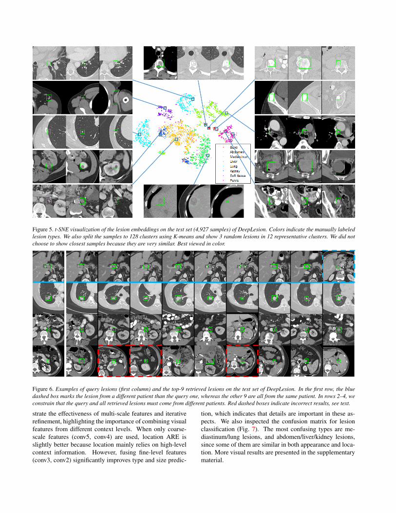
Figure 5. t-SNE visualization of the lesion embeddings on the test set (4,927 samples) of DeepLesion. Colors indicate the manually labeledlesion types. We also split the samples to 128 clusters using K-means and show 3 random lesions in 12 representative clusters. We did notchoose to show closest samples because they are very similar. Best viewed in color.

Figure 6. Examples of query lesions (first column) and the top-9 retrieved lesions on the test set of DeepLesion. In the first row, the bluedashed box marks the lesion from a different patient than the query one, whereas the other 9 are all from the same patient. In rows 2–4, weconstrain that the query and all retrieved lesions must come from different patients. Red dashed boxes indicate incorrect results, see text.

strate the effectiveness of multi-scale features and iterativerefinement, highlighting the importance of combining visualfeatures from different context levels. When only coarse-scale features (conv5, conv4) are used, location ARE isslightly better because location mainly relies on high-levelcontext information. However, fusing fine-level features(conv3, conv2) significantly improves type and size predic-

tion, which indicates that details are important in these as-pects. We also inspected the confusion matrix for lesionclassification (Fig. 7). The most confusing types are me-diastinum/lung lesions, and abdomen/liver/kidney lesions,since some of them are similar in both appearance and loca-tion. More visual results are presented in the supplementarymaterial.

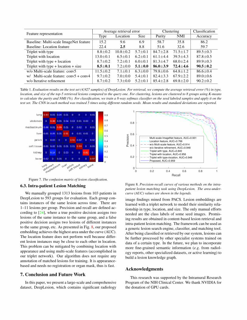
Feature representation Average retrieval error Clustering ClassificationType Location Size Purity NMI Accuracy

Baseline: Multi-scale ImageNet feature 15.2 9.6 6.9 58.7 35.8 86.2Baseline: Location feature 22.4 2.5 8.8 51.6 32.6 59.7Triplet with type 8.8±0.2 10.8±0.2 5.7±0.1 84.7±2.8 71.5±1.7 89.5±0.3Triplet with location 13.0±0.1 6.5±0.1 6.2±0.1 61.1±4.4 39.5±4.3 87.8±0.5Triplet with type + location 8.7±0.2 7.2±0.1 6.0±0.1 81.3±4.7 68.0±2.4 89.9±0.3Triplet with type + location + size 8.5±0.1 7.2±0.0 5.1±0.0 86.0±3.9 72.4±4.6 90.5±0.2w/o Multi-scale feature: conv5 11.5±0.2 7.1±0.1 6.3±0.0 79.8±0.6 64.8±1.2 86.6±0.4w/ Multi-scale feature: conv5 + conv4 9.7±0.2 7.0±0.0 5.4±0.1 82.4±3.3 67.9±2.2 89.0±0.6w/o Iterative refinement 8.7±0.2 7.3±0.0 5.2±0.1 85.4±2.8 69.8±2.0 90.2±0.2

Table 1. Evaluation results on the test set (4,927 samples) of DeepLesion. For retrieval, we compute the average retrieval error (%) in type,location, and size of the top-5 retrieved lesions compared to the query one. For clustering, lesions are clustered to 8 groups using K-meansto calculate the purity and NMI (%). For classification, we train a 8-way softmax classifier on the seed labeled samples and apply it on thetest set. The CNN in each method was trained 5 times using different random seeds. Mean results and standard deviations are reported.

Figure 7. The confusion matrix of lesion classification.

6.3. Intra-patient Lesion Matching

We manually grouped 1313 lesions from 103 patients inDeepLesion to 593 groups for evaluation. Each group con-tains instances of the same lesion across time. There are1–11 lesions per group. Precision and recall are defined ac-cording to [24], where a true positive decision assigns twolesions of the same instance to the same group, and a falsepositive decision assigns two lesions of different instancesto the same group, etc. As presented in Fig. 8, our proposedembedding achieves the highest area under the curve (AUC).The location feature does not perform well because differ-ent lesion instances may be close to each other in location.This problem can be mitigated by combining location withappearance and using multi-scale features (accomplished inour triplet network). Our algorithm does not require anyannotation of matched lesions for training. It is appearance-based and needs no registration or organ mask, thus is fast.

7. Conclusion and Future WorkIn this paper, we present a large-scale and comprehensive

dataset, DeepLesion, which contains significant radiology

0 0.2 0.4 0.6 0.8 1

Recall

0

0.2

0.4

0.6

0.8

1

Pre

cis

ion

Multi-scale ImageNet feature, AUC=0.931

Location feature, AUC=0.766

w/o Multi-scale feature, AUC=0.914

w/o Iterative refinement, AUC=0.948

Triplet with type, AUC=0.840

Triplet with location, AUC=0.958

Triplet with type+location, AUC=0.949

Proposed, AUC=0.959

Figure 8. Precision-recall curves of various methods on the intra-patient lesion matching task using DeepLesion. The area-under-curve (AUC) values are shown in the legends.

image findings mined from PACS. Lesion embeddings arelearned with a triplet network to model their similarity rela-tionship in type, location, and size. The only manual effortsneeded are the class labels of some seed images. Promis-ing results are obtained in content-based lesion retrieval andintra-patient lesion matching. The framework can be used asa generic lesion search engine, classifier, and matching tool.After being classified or retrieved by our system, lesions canbe further processed by other specialist systems trained ondata of a certain type. In the future, we plan to incorporatemore fine-grained semantic information (e.g. from radiol-ogy reports, other specialized datasets, or active learning) tobuild a lesion knowledge graph.

Acknowledgments

This research was supported by the Intramural ResearchProgram of the NIH Clinical Center. We thank NVIDIA forthe donation of GPU cards.

References[1] M. Belkin, P. Niyogi, and V. Sindhwani. Manifold regulariza-

tion: A geometric framework for learning from labeled andunlabeled examples. Journal of machine learning research,7(Nov):2399–2434, 2006. 5

[2] A. Bellet, A. Habrard, and M. Sebban. A survey on met-ric learning for feature vectors and structured data. arXivpreprint arXiv:1306.6709, 2013. 2

[3] J. Bromley, I. Guyon, Y. LeCun, E. Sackinger, and R. Shah.Signature verification using a “siamese” time delay neuralnetwork. In Advances in Neural Information Processing Sys-tems, pages 737–744, 1994. 2

[4] W. Chen, X. Chen, J. Zhang, and K. Huang. Beyond tripletloss: a deep quadruplet network for person re-identification.In CVPR, 2017. 2, 4

[5] X. Chen and A. Gupta. Webly supervised learning of convo-lutional networks. In Proceedings of the IEEE InternationalConference on Computer Vision, pages 1431–1439, 2015. 1

[6] J.-Z. Cheng, D. Ni, Y.-H. Chou, J. Qin, C.-M. Tiu, Y.-C.Chang, C.-S. Huang, D. Shen, and C.-M. Chen. Computer-Aided Diagnosis with Deep Learning Architecture: Applica-tions to Breast Lesions in US Images and Pulmonary Nodulesin CT Scans. Scientific Reports, 6(1):24454, jul 2016. 2

[7] K. Clark, B. Vendt, K. Smith, J. Freymann, J. Kirby, P. Kop-pel, S. Moore, S. Phillips, D. Maffitt, M. Pringle, L. Tarbox,and F. Prior. The Cancer Imaging Archive (TCIA): Maintain-ing and Operating a Public Information Repository. Journalof Digital Imaging, 26(6):1045–1057, dec 2013. 6

[8] S. Cornegruta, R. Bakewell, S. Withey, and G. Mon-tana. Modelling radiological language with bidirec-tional long short-term memory networks. arXiv preprintarXiv:1609.08409, 2016. 6

[9] J. Deng, W. Dong, R. Socher, L. J. Li, K. Li, and L. Fei-Fei. ImageNet: A large-scale hierarchical image database.In 2009 IEEE Conference on Computer Vision and PatternRecognition, pages 248–255, jun 2009. 1, 5

[10] E. Eisenhauer, P. Therasse, J. Bogaerts, L. H. Schwartz,D. Sargent, R. Ford, J. Dancey, S. Arbuck, S. Gwyther,M. Mooney, and Others. New response evaluation criteriain solid tumours: revised RECIST guideline (version 1.1).European journal of cancer, 45(2):228–247, 2009. 1, 3

[11] A. Esteva, B. Kuprel, R. A. Novoa, J. Ko, S. M. Swet-ter, H. M. Blau, and S. Thrun. Dermatologist-level classi-fication of skin cancer with deep neural networks. Nature,542(7639):115–118, 2017. 1, 2

[12] M. Everingham, L. Van Gool, C. K. Williams, J. Winn, andA. Zisserman. The pascal visual object classes (voc) chal-lenge. International journal of computer vision, 88(2):303–338, 2010. 1

[13] S. Gidaris and N. Komodakis. Object detection via a multi-region and semantic segmentation-aware cnn model. In Pro-ceedings of the IEEE International Conference on ComputerVision, pages 1134–1142, 2015. 5

[14] R. Girshick. Fast r-cnn. In Proceedings of the IEEE inter-national conference on computer vision, pages 1440–1448,2015. 4, 5

[15] H. Greenspan, B. van Ginneken, and R. M. Summers. GuestEditorial Deep Learning in Medical Imaging: Overview andFuture Promise of an Exciting New Technique. IEEE Trans-actions on Medical Imaging, 35(5):1153–1159, may 2016. 1,2

[16] J. Hofmanninger, M. Krenn, M. Holzer, T. Schlegl,H. Prosch, and G. Langs. Unsupervised identification ofclinically relevant clusters in routine imaging data. In In-ternational Conference on Medical Image Computing andComputer-Assisted Intervention, pages 192–200. Springer,2016. 2

[17] H. Hong, J. Lee, and Y. Yim. Automatic lung nodule match-ing on sequential CT images. Computers in Biology andMedicine, 38(5):623–634, may 2008. 2

[18] P. Hu and D. Ramanan. Finding Tiny Faces. In CVPR, 2017.5

[19] J. Krause, B. Sapp, A. Howard, H. Zhou, A. Toshev,T. Duerig, J. Philbin, and L. Fei-Fei. The unreasonable ef-fectiveness of noisy data for fine-grained recognition. InEuropean Conference on Computer Vision, pages 301–320.Springer, 2016. 1

[20] D.-H. Lee. Pseudo-label: The simple and efficient semi-supervised learning method for deep neural networks. InWorkshop on Challenges in Representation Learning, ICML,volume 3, page 2, 2013. 3

[21] Z. Li, X. Zhang, H. Muller, and S. Zhang. Large-scale re-trieval for medical image analytics: A comprehensive review.Medical Image Analysis, 43:66–84, jan 2018. 1, 2

[22] T.-Y. Lin, M. Maire, S. Belongie, J. Hays, P. Perona, D. Ra-manan, P. Dollar, and C. L. Zitnick. Microsoft coco: Com-mon objects in context. In European conference on computervision, pages 740–755. Springer, 2014. 1

[23] G. Litjens, T. Kooi, B. E. Bejnordi, A. A. A. Setio, F. Ciompi,M. Ghafoorian, J. A. van der Laak, B. van Ginneken, andC. I. Sanchez. A survey on deep learning in medical imageanalysis. Medical Image Analysis, 42:60–88, dec 2017. 1, 2

[24] C. D. Manning, P. Raghavan, and H. Schutze. Introductionto information retrieval. Cambridge University Press, 2008.6, 8

[25] J. H. Moltz, M. D’Anastasi, A. Kießling, D. P. Dos Santos,C. Schulke, and H.-O. Peitgen. Workflow-centred evaluationof an automatic lesion tracking software for chemotherapymonitoring by CT. European radiology, 22(12):2759–2767,2012. 2

[26] J. H. Moltz, M. Schwier, and H.-O. Peitgen. A general frame-work for automatic detection of matching lesions in follow-up ct. In Biomedical Imaging: From Nano to Macro, 2009.ISBI’09. IEEE International Symposium on, pages 843–846.IEEE, 2009. 2

[27] H. Oh Song, Y. Xiang, S. Jegelka, and S. Savarese. Deepmetric learning via lifted structured feature embedding. InProceedings of the IEEE Conference on Computer Vision andPattern Recognition, pages 4004–4012, 2016. 4

[28] J. Ramos, T. T. J. P. Kockelkorn, I. Ramos, R. Ramos, J. Grut-ters, M. A. Viergever, B. van Ginneken, and A. Campilho.Content-Based Image Retrieval by Metric Learning FromRadiology Reports: Application to Interstitial Lung Dis-

eases. IEEE Journal of Biomedical and Health Informatics,20(1):281–292, jan 2016. 2

[29] F. Schroff, D. Kalenichenko, and J. Philbin. Facenet: A uni-fied embedding for face recognition and clustering. In Pro-ceedings of the IEEE Conference on Computer Vision andPattern Recognition, pages 815–823, 2015. 2, 4

[30] A. A. A. Setio, A. Traverso, T. De Bel, M. S. Berens,C. van den Bogaard, P. Cerello, H. Chen, Q. Dou, M. E. Fan-tacci, B. Geurts, et al. Validation, comparison, and combina-tion of algorithms for automatic detection of pulmonary nod-ules in computed tomography images: the luna16 challenge.Medical Image Analysis, 42:1–13, 2017. 6

[31] M. Sevenster, A. R. Travis, R. K. Ganesh, P. Liu, U. Kose,J. Peters, and P. J. Chang. Improved efficiency in clin-ical workflow of reporting measured oncology lesions viapacs-integrated lesion tracking tool. American Journal ofRoentgenology, 204(3):576–583, 2015. 2

[32] H.-C. Shin, L. Lu, L. Kim, A. Seff, J. Yao, and R. Summers.Interleaved text/image deep mining on a large-scale radiol-ogy database for automated image interpretation. Journal ofMachine Learning Research, 17(1-31):2, 2016. 6

[33] H.-C. Shin, H. R. Roth, M. Gao, L. Lu, Z. Xu, I. Nogues,J. Yao, D. Mollura, and R. M. Summers. Deep ConvolutionalNeural Networks for Computer-Aided Detection: CNN Ar-chitectures, Dataset Characteristics and Transfer Learning.IEEE Transactions on Medical Imaging, 35(5):1285–1298,may 2016. 2

[34] J. S. Silva, J. Cancela, and L. Teixeira. Fast volumetric reg-istration method for tumor follow-up in pulmonary ct exams.Journal of Applied Clinical Medical Physics, 12(2):362–375,2011. 2

[35] K. Simonyan and A. Zisserman. Very deep convolutionalnetworks for large-scale image recognition. In ICLR 2015,2015. 5

[36] K. Sohn. Improved Deep Metric Learning with Multi-classN-pair Loss Objective. In Neural Information ProcessingSystems, pages 1–9, 2016. 2

[37] J. Son, M. Baek, M. Cho, and B. Han. Multi-Object Track-ing with Quadruplet Convolutional Neural Networks. In Pro-ceedings of the IEEE Conference on Computer Vision andPattern Recognition, pages 5620–5629, 2017. 2, 4

[38] H. O. Song, S. Jegelka, V. Rathod, and K. Murphy. Deepmetric learning via facility location. In IEEE CVPR, 2017. 2

[39] N. Tajbakhsh, J. Y. Shin, S. R. Gurudu, R. T. Hurst, C. B.Kendall, M. B. Gotway, and J. Liang. Convolutional Neu-ral Networks for Medical Image Analysis: Full Trainingor Fine Tuning? IEEE Transactions on Medical Imaging,35(5):1299–1312, may 2016. 2

[40] A. Teramoto, H. Fujita, O. Yamamuro, and T. Tamaki. Au-tomated detection of pulmonary nodules in pet/ct images:Ensemble false-positive reduction using a convolutional neu-ral network technique. Medical physics, 43(6):2821–2827,2016. 2, 5

[41] L. Tsochatzidis, K. Zagoris, N. Arikidis, A. Karahaliou,L. Costaridou, and I. Pratikakis. Computer-aided diagnosis ofmammographic masses based on a supervised content-basedimage retrieval approach. Pattern Recognition, 2017. 2

[42] L. van der Maaten. Accelerating t-SNE using Tree-Based Al-gorithms. Journal of Machine Learning Research, 15:3221–3245, 2014. 6

[43] R. Vivanti. Automatic liver tumor segmentation in follow-up ct studies using convolutional neural networks. In Proc.Patch-Based Methods in Medical Image Processing Work-shop, 2015. 2

[44] X. Wang, L. Lu, H.-C. Shin, L. Kim, M. Bagheri, I. Nogues,J. Yao, and R. M. Summers. Unsupervised joint mining ofdeep features and image labels for large-scale radiology im-age categorization and scene recognition. In Applications ofComputer Vision (WACV), 2017 IEEE Winter Conference on,pages 998–1007. IEEE, 2017. 2, 5

[45] X. Wang, Y. Peng, L. Lu, Z. Lu, M. Bagheri, and R. M. Sum-mers. ChestX-ray8: Hospital-scale Chest X-ray Databaseand Benchmarks on Weakly-Supervised Classification andLocalization of Common Thorax Diseases. In CVPR, may2017. 6

[46] Z. Wang, Y. Yin, J. Shi, W. Fang, H. Li, and X. Wang. Zoom-in-Net: Deep Mining Lesions for Diabetic Retinopathy De-tection, pages 267–275. Springer International Publishing,2017. 1, 2

[47] G. Wei, H. Ma, W. Qian, and M. Qiu. Similarity measure-ment of lung masses for medical image retrieval using ker-nel based semisupervised distance metric. Medical Physics,43(12):6259–6269, nov 2016. 2

[48] H. Zhang, X. Shang, W. Yang, H. Xu, H. Luan, and T.-S.Chua. Online collaborative learning for open-vocabulary vi-sual classifiers. In Proceedings of the IEEE Conference onComputer Vision and Pattern Recognition, pages 2809–2817,2016. 1

[49] X. Zhang, F. Zhou, Y. Lin, and S. Zhang. Embedding labelstructures for fine-grained feature representation. In Proceed-ings of the IEEE Conference on Computer Vision and PatternRecognition, pages 1114–1123, 2016. 2, 4

[50] Z. Zhang, Y. Xie, F. Xing, M. McGough, and L. Yang. MD-Net: A Semantically and Visually Interpretable Medical Im-age Diagnosis Network. In CVPR, 2017. 6

[51] X. Zhu and Z. Ghahramani. Learning from labeled and un-labeled data with label propagation. Technical Report CMU-CALD-02-107, Carnegie Mellon University, 2002. 5

Supplementary Material

In this material, we provide some additional illustrationsof the paper. Sec. 1 visualizes the DeepLesion dataset anddescribes some details. Sec. 2 provides implementationdetails of the self-supervised body-part regressor. Morecontent-based lesion retrieval results are presented in Sec. 3.Sec. 4 illustrates the intra-patient lesion matching task andthe intra-patient lesion graph.

1. DeepLesion Dataset: Visualization and De-tails

To provide an overview of the DeepLesion dataset, wedraw a scatter map to show the distribution of the typesand relative body locations of the lesions in Fig. 3. Fromthe lesion types and sample images, one can see that therelative body locations of the lesions are consistent withtheir actual physical positions, proving the validity of thelocation information used in the paper, particularly the self-supervised body-part regressor. Some lesion types like bone

Long diameter = 78.6 mm

Short diameter = 58.8 mm

z = 0.59 (from SSBR)

x = 0.28, y = 0.53 (relative)

Figure 1. Location and size of a sample lesion. The red lines arethe long and short diameters annotated by radiologists during theirdaily work. The green box is the bounding box calculated from thediameters. The yellow dot is the center of the bounding box. Theblue lines indicate the relative x- and y-coordinates of the lesion.The z-coordinate is predicted by SSBR. Best viewed in color.

0 10 20 30 40 50 60 70 80

Long diameter (mm)

0

2000

4000

(a)

0 10 20 30 40 50 60 70 80

Short diameter (mm)

0

2000

4000

(b)

1 1.5 2 2.5 3

Ratio (Long/Short)

0

5000

10000# S

am

ple

s

(c)

Figure 2. Distribution of the lesion-sizes in DeepLesion. For clarity,values greater than the upper bound of the x-axis of each plot aregrouped in the last bin of each histogram.

and soft tissue have widespread locations. Neighboring typessuch as lung/mediastinum and abdomen/liver/kidney havelarge overlap in location due to inter-subject variabilities.Besides, we can clearly see the considerable diversity ofDeepLesion.

Fig. 1 illustrates the approach to obtain the location andsize of a lesion. In order to locate a lesion in the body, wefirst obtain the mask of the body in the axial slice, thencompute the relative position (0–1) of the lesion center to getthe x- and y-coordinates. As for z, the self-supervised body-part regressor (SSBR) is used. We also show the distributionof the lesion-sizes in Fig. 2.

1

a

b

c

d

e

f

g

h i j k l

m

n

o

p

q

r

stuv

Figure 3. Visualization of the DeepLesion dataset (test set). The x- and y-axes of the scatter map correspond to the x- and z-coordinates ofthe relative body location of each lesion, respectively. Therefore, this map is similar to a frontal view of the human body. Colors indicate themanually labeled lesion types. Sample lesions are exhibited to show the great diversity of DeepLesion, including: a. lung nodule; b. lungcyst; c. costophrenic sulcus (lung) mass/fluid; d. breast mass; e. liver lesion; f. renal mass; g. large abdominal mass; h. posterior thigh mass; i.iliac sclerotic lesion; j. perirectal lymph node (LN); k. pelvic mass; l. periportal LN; m. omental mass; n. peripancreatic lesion; o. spleniclesion; p. subcutaneous/skin nodule; q. ground glass opacity; r. axillary LN; s. subcarinal LN; t. vertebral body metastasis; u. thyroid nodule;v. neck mass.

2. Self-Supervised Body-Part Regressor: Im-plementation Details

To train SSBR, we randomly pick 800 unlabeled CT vol-umes of 420 subjects from DeepLesion. Each axial slicein the volumes is resized to 128 × 128 pixels. No furtherpreprocessing or data augmentation was performed. In eachmini-batch, we randomly select 256 slices from 32 volumes(8 equidistant slices in each volume, see Eq. 2 in the paper)for training. The network is trained using stochastic gradientdescent with a learning rate of 0.002. It generally convergesin 1.5K iterations.

The sample lesions in Fig. 3 can be used to qualitativelyevaluate the learned slice scores, or z-coordinates. We alsoconducted a preliminary experiment to quantitatively assessSSBR. A test set including 18,195 slices subsampled from260 volumes of 140 new subjects are collected. They aremanually labeled as one of the 3 classes: chest (5903 slices),abdomen (6744), or pelvis (5548). The abdomen class startsfrom the upper border of the liver and ends at the upperborder of the ilium. Then, we set two thresholds on the slicescores to classify them to the three classes. The classifica-tion accuracy is 95.99%, with all classification errors appear-ing at transition regions (chest-abdomen, abdomen-pelvis)partially because of their ambiguity. The result proves theeffectiveness of SSBR. More importantly, SSBR is trainedon unlabeled volumes that are abundant in every hospital’sdatabase, thus zero annotation effort is needed.

3. Content-based Lesion Retrieval: More Re-sults

More examples of lesion retrieval are shown in Fig. 4. Wetry to exhibit typical examples of all lesion types. The lastrow is a failure case. Most retrieved lesions are similar withthe query ones in type, location, and size. More importantly,most retrieved lesions and the query ones come from seman-tically similar body structures that are not specified in thetraining labels. The failure cases in Fig. 4 have dissimilartypes with the query ones. They were retrieved mainly be-cause they have similar location, size, and appearance withquery ones.

(a)

(b)

(c)

(d)

(e)

(f)

(g)

(h)

(i)

Query

Figure 4. More examples of query lesions (first column) and the top-9 retrieved lesions on the test set of DeepLesion. We constrain that thequery and all retrieved lesions must come from different patients. Red dashed boxes indicate incorrect results. The lesions in each row are:(a) Right axillary lymph nodes; (b) subcarinal lymph nodes; (c) lung masses or nodules near the pleura; (d) liver lesions near the liver dome;(e) right kidney lesions; (f) lesions near the anterior abdomen wall; (g) lesions on pelvic bones except the one in the red box, which is aperipherally calcified mass. (h) inferior pelvic lesions; (i) spleen lesions except the ones in red boxes.

4. Intra-Patient Lesion Matching: An Example

To provide a intuitive illustration of the lesion matchingtask, we show lesions of a sample patient in Fig. 5, with their

lesion graph in Fig. 6 and the final extracted lesion sequencesin Fig. 7. We show that the lesion graph and Algo. 1 in thepaper can be used to accurately match lesions in multiplestudies.

1 1 1

1

2

3

4

Study 1 Study 2 Study 3 Study 4 Study 5

Figure 5. All lesions of a sample patient in DeepLesion. Lesions in each study (CT examination) are listed in a column. Not all lesionsoccur in each study, because the scan ranges of each study vary and radiologists only mark a few target lesions. We group the same lesioninstances to sequences. Four sequences are found and marked in the figure, where the numbers on the connections represent the lesion IDs.

0.320.33

0.36 0.37

0.40

0.310.37 0.32

0.34 0.250.27

0.34

0.21

Figure 6. The intra-patient lesion graph of the patient in Fig. 5. Forclarity, the lesions in Fig. 5 are replaced by nodes in this figure. Thenumbers on the edges are the Euclidean distances between nodes.We only show small distances in the figure. Red, thick edgesindicate smaller distances. Note that some edges may overlap withother edges or nodes.

0.32

0.40

0.31

0.340.27

0.34

0.21

Figure 7. The final lesion sequences found by processing the lesiongraph in Fig. 6 using Algo. 1 in the paper. They are the same withthe ground-truth in Fig. 5.