deep learning - umd department of computer science | · 2017-05-13 · • deep learning...

Deep Learning

CMSC 422

MARINE CARPUAT

[email protected] on slides by Vlad Morariu

mailto:[email protected]

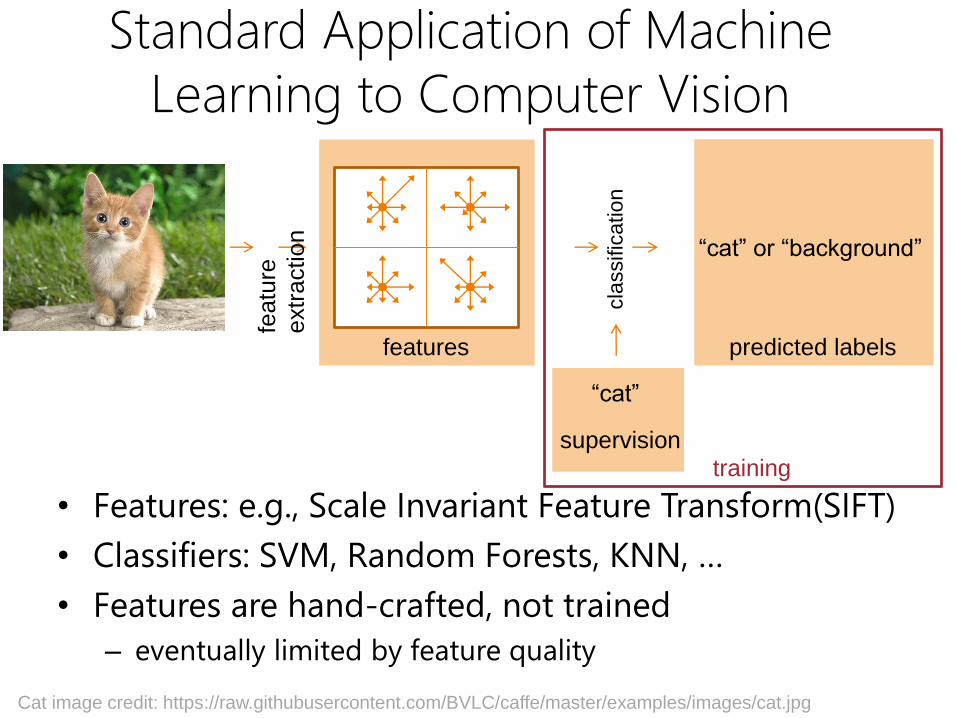
Standard Application of Machine

Learning to Computer Vision

• Features: e.g., Scale Invariant Feature Transform(SIFT)

• Classifiers: SVM, Random Forests, KNN, …

• Features are hand-crafted, not trained

– eventually limited by feature quality

featu

re

extr

action

features

cla

ssific

ation

“cat” or “background”

predicted labels

“cat”

supervisiontraining

Cat image credit: https://raw.githubusercontent.com/BVLC/caffe/master/examples/images/cat.jpg

• Deep learning– multiple layer neural networks

– learn features and classifiers directly (“end-to-end”

training)

– breakthrough in Computer Vision, now in other AI areas

Image credit: LeCun, Y., Bottou, L., Bengio, Y., Haffner, P. “Gradient-based learning applied to

document recognition.” Proceedings of the IEEE, 1998.

training

features classifier

supervision

Speech Recognition

Slide credit: Bohyung Han

Image Classification Performance

Image Classification Top-5 Errors (%)

Slide credit: Bohyung HanFigure from: K. He, X. Zhang, S. Ren, J. Sun. “Deep Residual

Learning for Image Recognition”. arXiv 2015. (slides)

Today’s lecture: key concepts

• Convolutional Neural Networks

• Revisiting Backpropagation and Gradient

Descent for Deep Networks

Multi-Layer Perceptron (MLP)

Image source: http://cs231n.github.io/neural-networks-1/

Neural Networks Applied to VisionLeCun, Y; Boser, B; Denker, J; Henderson, D; Howard, R; Hubbard, W; Jackel, L, “Backpropagation Applied to Handwritten Zip Code Recognition,” in Neural Computation, 1989

– USPS digit recognition, later check reading

– Convolution, pooling (“weight sharing”), fully connected layers



Architecture overview

Components:

– Convolution layers

– Pooling/Subsampling layers

– Fully connected layers



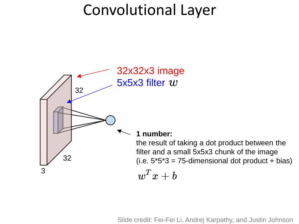
Convolutional Layer

32

32

3

32x32x3 image

width

height

depth

Slide credit: Fei-Fei Li, Andrej Karpathy, and Justin Johnson

11 Jan 201632

32

3

5x5x3 filter

32x32x3 image

Convolve the filter with the image

i.e. “slide over the image spatially,

computing dot products”

Convolutional Layer


11 Jan 201632

32

3

5x5x3 filter

32x32x3 image

Convolve the filter with the image

i.e. “slide over the image spatially,

computing dot products”

Filters always extend the full

depth of the input volume

Convolutional Layer


11 Jan 201632

32

3

32x32x3 image

5x5x3 filter

1 number:

the result of taking a dot product between the

filter and a small 5x5x3 chunk of the image

(i.e. 5*5*3 = 75-dimensional dot product + bias)

Convolutional Layer


11 Jan 201632

32

3

32x32x3 image

5x5x3 filter

convolve (slide) over all

spatial locations

activation map

1

28

28

Convolutional Layer


11 Jan 201632

32

3

32x32x3 image

5x5x3 filter

convolve (slide) over all

spatial locations

activation maps

1

28

28

consider a second, green filter

Convolutional Layer


11 Jan 201632

32

3

Convolution Layer

activation maps

6

28

28

For example, if we had 6 5x5 filters, we’ll get 6 separate activation maps:

We stack these up to get a “new image” of size 28x28x6!

Convolutional Layer


11 Jan 2016

ConvNet is a sequence of Convolutional Layers, interspersed with activation

functions

32

32

3

28

28

6

CONV,

ReLU

e.g. 6

5x5x3

filters

Convolutional Layer


11 Jan 2016

ConvNet is a sequence of Convolutional Layers, interspersed with activation

functions

32

32

3

CONV,

ReLU

e.g. 6

5x5x3

filters 28

28

6

CONV,

ReLU

e.g. 10

5x5x6

filters

CONV,

ReLU

….

10

24

24

Convolutional Layer


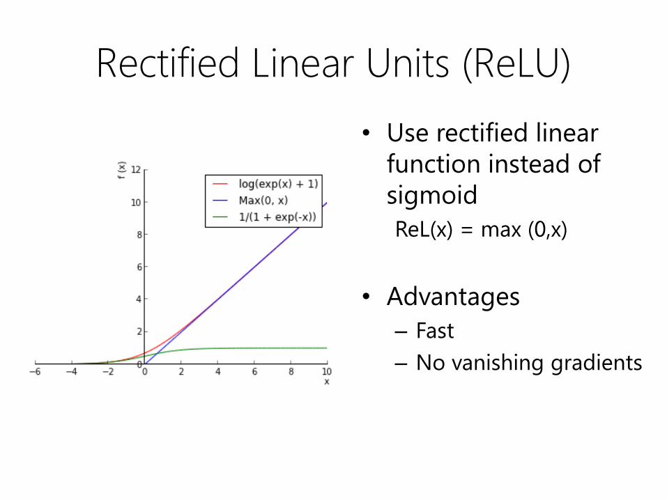
Rectified Linear Units (ReLU)

• Use rectified linear

function instead of

sigmoid

ReL(x) = max (0,x)

• Advantages

– Fast

– No vanishing gradients

11 Jan 2016

- makes the representations smaller and more manageable

- operates over each activation map independently

Pooling Layer


11 Jan 2016

1 1 2 4

5 6 7 8

3 2 1 0

1 2 3 4

Single depth slice

x

y

max pool with 2x2 filters

and stride 2 6 8

3 4

MAX POOLING

Pooling Layer


11 Jan 2016

[From recent

Yann LeCun

slides]

Convolutional filter visualization


11 Jan 2016

example 5x5 filters(32 total)

We call the layer convolutional

because it is related to convolution

of two signals:

elementwise multiplication

and sum of a filter and the

signal (image)

one filter =>

one activation map

Convolutional filter visualization


Today’s lecture: key concepts




Multi-Layer Perceptron (MLP)

Image source: http://cs231n.github.io/neural-networks-1/

Single neuron gradient𝑥1

𝚺Sigmoid

𝑥2

𝑥𝑑

𝑏𝑤1

𝑤2

𝑤𝑑

𝑧 𝑦

𝑧 = 𝑏 +

𝑖

𝑤𝑖𝑥𝑖

𝓛

𝑦

𝐿

𝑦 =1

1 + 𝑒−𝑧𝐿 =

1

2

𝑛

𝑦𝑛 − 𝑦𝑛 2

𝜕𝐿

𝜕 𝑦𝑛 = − 𝑦𝑛 − 𝑦𝑛

𝑛

𝜕 𝑦𝑛

𝜕𝑤𝑖

𝜕𝐿

𝜕 𝑦𝑛=

𝑛

𝜕𝑧𝑛

𝜕𝑤𝑖

𝑑 𝑦𝑛

𝑑𝑧𝑛

𝜕𝐿

𝜕 𝑦𝑛= −

𝑛

𝑥𝑖𝑛 𝑦𝑛 1 − 𝑦𝑛 𝑦𝑛 − 𝑦𝑛

𝑑 𝑦

𝑑𝑧= 𝑦(1 − 𝑦)

𝜕𝑧

𝜕𝑤𝑖= 𝑥𝑖

𝜕𝐿

𝜕𝑤𝑖=

Slide credit: Adapted from Bohyung Han

Chain rule:

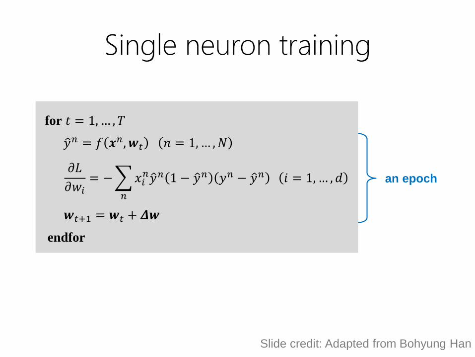
Single neuron training

𝜕𝐿

𝜕𝑤𝑖= −

𝑛

𝑥𝑖𝑛 𝑦𝑛 1 − 𝑦𝑛 𝑦𝑛 − 𝑦𝑛 𝑖 = 1,… , 𝑑

for 𝑡 = 1, … , 𝑇

𝒘𝑡+1 = 𝒘𝑡 + 𝜟𝒘

𝑦𝑛 = 𝑓 𝒙𝑛, 𝒘𝑡 𝑛 = 1,… ,𝑁

endfor

an epoch

Slide credit: Adapted from Bohyung Han

Multi-Layer: Backpropagation

28

Neuron 𝑗Neuron 𝑖

𝑥𝑘 𝚺Sigmoid

𝑤𝑘𝑖 𝑧𝑖𝓛

𝑦

𝐿 𝑦𝑖 𝚺Sigmoid

𝑧𝑗 𝑦𝑗

𝑤𝑖𝑗

𝜕𝐿

𝜕 𝑦𝑖=

𝑗

𝑑𝑧𝑗

𝑑 𝑦𝑖

𝜕𝐿

𝜕𝑧𝑗=

𝑗

𝑤𝑖𝑗

𝜕𝐿

𝜕𝑧𝑗

𝜕𝐿

𝜕𝑤𝑘𝑖=

𝑛

𝜕𝑧𝑖𝑛

𝜕𝑤𝑘𝑖

𝑑 𝑦𝑖𝑛

𝑑𝑧𝑖𝑛

𝜕𝐿

𝜕 𝑦𝑖𝑛

𝜕𝐿

𝜕𝑧𝑗=

𝑑 𝑦𝑗

𝑑𝑧𝑗

𝜕𝐿

𝜕 𝑦𝑗

=

𝑛

𝜕𝑧𝑖𝑛

𝜕𝑤𝑘𝑖

𝑑 𝑦𝑖𝑛

𝑑𝑧𝑖𝑛

𝑗

𝑤𝑖𝑗

𝑑 𝑦𝑗𝑛

𝑑𝑧𝑗𝑛

𝜕𝐿

𝜕 𝑦𝑗𝑛

=

𝑗

𝑤𝑖𝑗

𝑑 𝑦𝑗

𝑑𝑧𝑗

𝜕𝐿

𝜕 𝑦𝑗


Backpropagation in practice

Two passes per iteration:

• Forward pass: compute value of loss function (and intermediate neurons) given inputs

• Backward pass: propagate gradient of loss (error) backwards through the network using the chain rule

Stochastic Gradient Descent (SGD)• Update weights for each sample

• Minibatch SGD: Update weights for a small set of samples

𝐸 =1

2𝑦𝑛 − 𝑦𝑛 2 𝒘𝑖 𝑡 + 1 = 𝒘𝑖 𝑡 − 𝜖

𝜕𝐸𝑛

𝜕𝒘𝑖

𝐸 =1

2

𝑛∈𝐵

𝑦𝑛 − 𝑦𝑛 2 𝒘𝑖 𝑡 + 1 = 𝒘𝑖 𝑡 − 𝜖𝜕𝐸𝐵

𝜕𝒘𝑖

+ Fast, online− Sensitive to noise

+ Fast, online+ Robust to noise


SGD improvements: Momentum

• Remember the previous direction

𝑣𝑖 𝑡 = 𝛼𝑣𝑖 𝑡 − 1 − 𝜖𝜕𝐸

𝜕𝑤𝑖(𝑡)

𝒘 𝑡 + 1 = 𝒘 𝑡 + 𝒗(𝑡)

+ Converge faster+ Avoid oscillation


SGD improvements: Weight Decay

• Penalize the size of the weights

𝑤𝑖 𝑡 + 1 = 𝑤𝑖 𝑡 − 𝜖𝜕𝐶

𝜕𝑤𝑖= 𝑤𝑖 𝑡 − 𝜖

𝜕𝐸

𝜕𝑤𝑖− 𝜆𝑤𝑖

𝐶 = 𝐸 +1

2

𝑖

𝑤𝑖2

+ Improve generalization a lot!


Key concepts




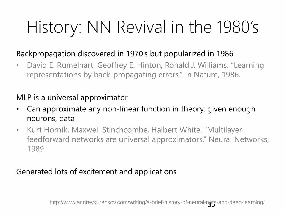
History: NN Revival in the 1980’s

Backpropagation discovered in 1970’s but popularized in 1986

• David E. Rumelhart, Geoffrey E. Hinton, Ronald J. Williams. “Learning

representations by back-propagating errors.” In Nature, 1986.

MLP is a universal approximator

• Can approximate any non-linear function in theory, given enough

neurons, data

• Kurt Hornik, Maxwell Stinchcombe, Halbert White. “Multilayer

feedforward networks are universal approximators.” Neural Networks,

1989

Generated lots of excitement and applications

35http://www.andreykurenkov.com/writing/a-brief-history-of-neural-nets-and-deep-learning/

Neural Networks Applied to Vision

LeNet – vision application– LeCun, Y; Boser, B; Denker, J; Henderson, D; Howard, R; Hubbard,

W; Jackel, L, “Backpropagation Applied to Handwritten Zip Code Recognition,” in Neural Computation, 1989

– USPS digit recognition, later check reading

– Convolution, pooling (“weight sharing”), fully connected layers



Issues in Deep Neural Networks

• Prohibitive training time

– Especially with lots of training data

– Many epochs typically required for optimization

– Expensive gradient computations

• Overfitting

– Learned function fits training data well, but

performs poorly on new data (high capacity

model, not enough training data)

Slide credit: adapted from Bohyung Han

Issues in Deep Neural Networks

Vanishing gradient problem

– Gradients in the lower layers are typically extremely small

– Optimizing multi-layer neural networks takes huge amount of time

𝜕𝐸

𝜕𝑤𝑘𝑖=

𝑛

𝜕𝑧𝑖𝑛

𝜕𝑤𝑘𝑖

𝑑 𝑦𝑖𝑛

𝑑𝑧𝑖𝑛

𝜕𝐸

𝜕 𝑦𝑖𝑛 =

𝑛

𝜕𝑧𝑖𝑛

𝜕𝑤𝑘𝑖

𝑑 𝑦𝑖𝑛

𝑑𝑧𝑖𝑛

𝑗

𝑤𝑖𝑗

𝑑 𝑦𝑗𝑛

𝑑𝑧𝑗𝑛

𝜕𝐸

𝜕 𝑦𝑗𝑛

Sigmoid

𝑧 𝑦

Slide credit: adapted from Bohyung Han

New “winter” and revival in early 2000’s

New “winter” in the early 2000’s due to

• problems with training NNs

• Support Vector Machines (SVMs), Random Forests (RF) – easy

to train, nice theory

Revival again by 2011-2012

• Name change (“neural networks” -> “deep learning”)

• + Algorithmic developments

– unsupervised layer-wise pre-training

– ReLU, dropout, layer normalizatoin

• + Big data + GPU computing =

• Large outperformance on many datasets (Vision: ILSVRC’12)

http://www.andreykurenkov.com/writing/a-brief-history-of-neural-nets-and-deep-learning-part-4/

Big Data• ImageNet Large Scale Visual Recognition Challenge

– 1000 categories w/ 1000 images per category

– 1.2 million training images, 50,000 validation, 150,000 testing

40O. Russakovsky, J. Deng, H. Su, J. Krause, S. Satheesh, S. Ma, Z. Huang, A. Karpathy, A. Khosla,

M. Bernstein, A. C. Berg and L. Fei-Fei. ImageNet Large Scale Visual Recognition Challenge. IJCV, 2015.

AlexNet Architecture

60 million parameters!

Various tricks

• ReLU nonlinearity

• Overlapping pooling

• Local response normalization

• Dropout – set hidden neuron output to 0 with probability .5

• Data augmentation

• Training on GPUs

Alex Krizhevsky, Ilya Sutskeyer, Geoffrey E. Hinton. ImageNet Classification with Deep Convolutional Neural Networks. NIPS, 2012.

Figure credit: Krizhevsky et al, NIPS 2012.

GPU Computing

• Big data and big models require lots of

computational power

• GPUs

– thousands of cores for parallel operations

– multiple GPUs

– still took about 5-6 days to train AlexNet on

two NVIDIA GTX 580 3GB GPUs (much faster

today)

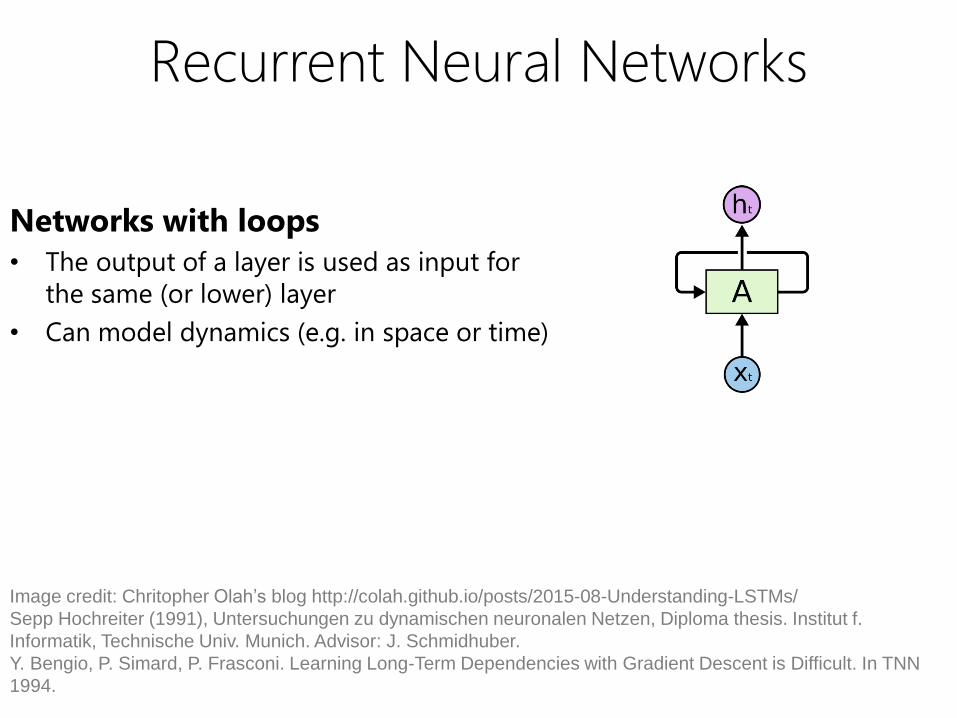
Recurrent Neural Networks

Networks with loops

• The output of a layer is used as input for

the same (or lower) layer

• Can model dynamics (e.g. in space or time)

Image credit: Chritopher Olah’s blog http://colah.github.io/posts/2015-08-Understanding-LSTMs/

Sepp Hochreiter (1991), Untersuchungen zu dynamischen neuronalen Netzen, Diploma thesis. Institut f.

Informatik, Technische Univ. Munich. Advisor: J. Schmidhuber.

Y. Bengio, P. Simard, P. Frasconi. Learning Long-Term Dependencies with Gradient Descent is Difficult. In TNN

1994.

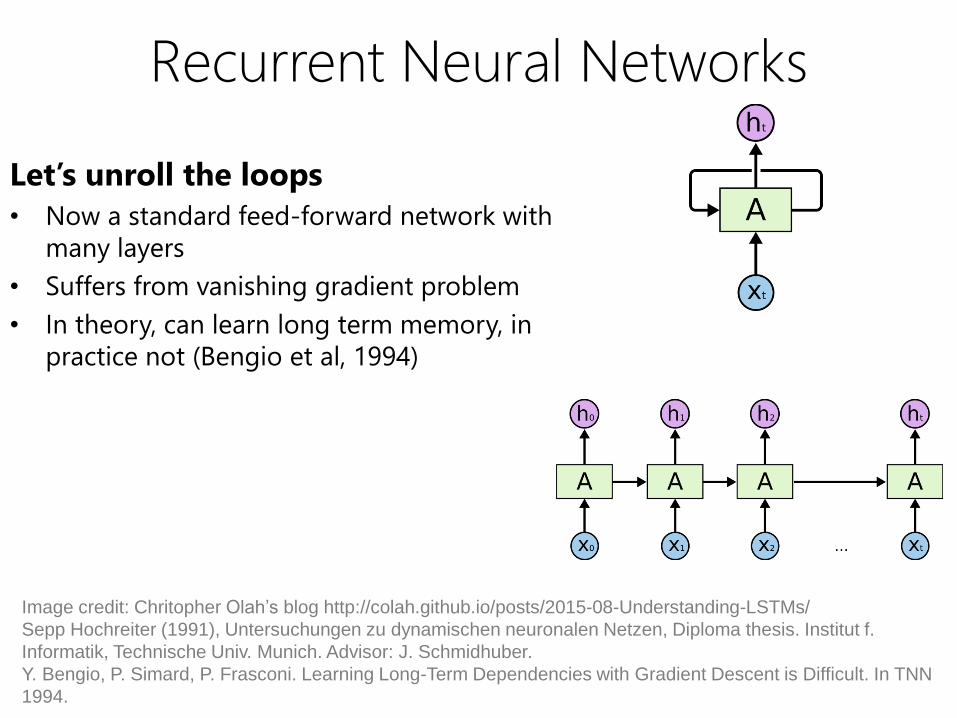
Recurrent Neural Networks

Let’s unroll the loops

• Now a standard feed-forward network with

many layers

• Suffers from vanishing gradient problem

• In theory, can learn long term memory, in

practice not (Bengio et al, 1994)

Image credit: Chritopher Olah’s blog http://colah.github.io/posts/2015-08-Understanding-LSTMs/

Sepp Hochreiter (1991), Untersuchungen zu dynamischen neuronalen Netzen, Diploma thesis. Institut f.

Informatik, Technische Univ. Munich. Advisor: J. Schmidhuber.

Y. Bengio, P. Simard, P. Frasconi. Learning Long-Term Dependencies with Gradient Descent is Difficult. In TNN

1994.

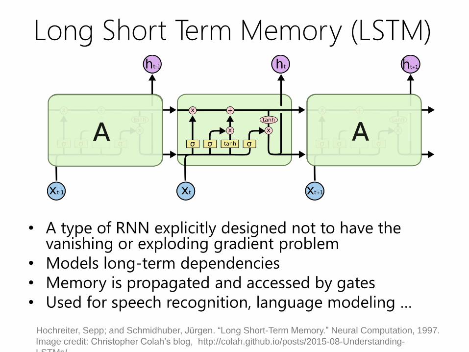
Long Short Term Memory (LSTM)

• A type of RNN explicitly designed not to have the vanishing or exploding gradient problem

• Models long-term dependencies

• Memory is propagated and accessed by gates

• Used for speech recognition, language modeling …

Hochreiter, Sepp; and Schmidhuber, Jürgen. “Long Short-Term Memory.” Neural Computation, 1997.

Image credit: Christopher Colah’s blog, http://colah.github.io/posts/2015-08-Understanding-

LSTMs/

Unsupervised Neural Networks

Autoencoders

• Encode then decode the

same input

• No supervision needed

input x

hidden layer

output x’

H. Bourlard and Y. Kamp. 1988. Auto-association by multilayer perceptrons and singular value decomposition.

Biol. Cybern. 59, 4-5 (September 1988), 291-294.

deep learning - umd department of computer science | · 2017-05-13 · • deep learning...

Documents