A Study On Deep Learning

Abdelrahman HosnyGraduate Student, Master’s

Computer ScienceUniversity of Connecticut

Email: abdelrahman@engr.uconn.edu

Anthony ParzialeUndergraduate Student, Junior

Computer ScienceUniversity of Connecticut

Email: anthony.parziale@uconn.edu

Abstract—With massive amounts of computational power, ma-chines can now recognize objects and translate speech in realtime. Thanks to Deep Learning, Artificial Intelligence is nowgetting smart. Deep Learning models attempt to mimic theactivity of the neocortex. It is understood that the activity ofthese layers of neurons is what constitutes a brain to be ableto ”think.” These models learn to recognize patterns in digitalrepresentations of data in a very similar sense to humans. Inthis survey report, we introduce the most important conceptsof Deep Learning along with the state of the art models thatare now widely adopted in commercial products.

1. Introduction

Machine learning is the science of getting computersto act without being explicitly programmed. It is the mainengine to many of the modern software applications: fromweb searches to content filtering on social networks torecommendations on e-commerce websites and smartphoneapplications. Deep learning is a new area of machine learn-ing research, which has been introduced with the objectiveof moving machine learning closer to one of its originalgoals: Artificial Intelligence. When exploring the field ofdeep learning, it is easy to be overwhelmed with variousmodels and in the process, lose sight of the end objective [1].Researchers aim at utilizing deep learning models to makeprogress toward human-level AI. Many of them view deeplearning is a direct extension to artificial neural networks,that are inspired by how the human brain works.

In this survey, our aim is to provide a brief explanation ofneural networks in addition to a concise explanation of thediffering deep learning architectures, their objectives, andhow they relate. In the next section, we start with the build-ing block of any deep learning architecture: Artificial NeuralNetworks. After that, we explore Deep learning models thatgenerally either consist of a ”deep” neural network (morethan 3 layers), or a stack of neural networks (where eachlayer in the deep architecture is in fact a neural networkitself). In each model introduced, we shed the light on thepurpose of the model and its architecture. At the end, wegive practical tips on using each model and introduce someof the recent commercial applications that are empoweredby deep learning models.

2. Artificial Neural Networks

Artificial neural networks are a family of models thatare inspired by biological neural networks. The idea behindartificial neural network is the observation that babies seeadults moving around and after a few months, the accu-mulated knowledge start to stimulate them to make mini-pushups. This behavior encouraged neuroscientists to studythe activity that happens in their brains to learn withoutbeing explicitly taught. In a similar analogy, computer sci-entists modeled the brain in a mathematical model called:artificial neural network. The question now is: how does thebrain work?

2.1. Background

Brains consist of neural cells. Each cell of these lookslike the one in figure 1. In the body of the neuron, thereis the nucleus that receives pulses of electricity from inputwires (dendrites) and based on these signals, the neurondoes some computation and sends a message (electricalimpulses) to other neurons through output wires (axons).The human brain has billions of these neurons connectedtogether. Different neurons in the brain are responsible fordifferent senses, like the sight, smell and touch senses. Itis scientifically observed that any neuron in the brain netcan learn to do other jobs. For example, experiments onanimals prove that if we disconnect the wires that connectan auditory neuron to the ears and connect it to the eyes, the

Figure 1: Human Brain Neuron

(a) Auditory cortex learns to see (b) Somatosensory cortex learns to see

Figure 2: Neurons learn to do different tasks when original wires are disconnected and reconnected to other senses

neuron will learn to see as in figure 2a. Similar experimentsdisconnect the somatosensory neuron connection to the handand connect it to the eyes, it will eventually learn to see as infigure 2b. Now, let’s switch context to talk about mimickingthis neural network in computers.

In a software environment, we create a similar modelthat has the three major components:

• Cell body that contains the neuron. This neuron isresponsible for doing the computations.

• Input wires that carry out signals as inputs.• Output wire(s) that transfer the output signal to other

neurons.

Figure 3 is a simple artificial (computer-one) neuralnetwork that has only one neuron (the orange circle). x1, x2,and x3 are the inputs to the neuron and they carry numericalvalues. The function h is called the hypothesis function. Itcomputes its value by multiplying the input vector x by awight vector w and then the output is passed through anactivation function that computes the final scalar output

Figure 3: Artificial neural network with one neuron

Figure 4 shows a more advanced neural network. Eachvertical set of neurons is called a layer. Layer 1 contains theneurons that represent inputs. Layer 2 is also called a hiddenlayer. It does the core computation. Layer 3 is called theoutput layer and does a computation on the data receivedfrom layer 2 and then outputs one final result. Now, themissing information in the one-neuron figure is:

1) What is the weight vector to be multiplied by theinput vector?

2) After multiplying the two vectors, what is the acti-vation function that will output the final result?

Besides the number of layers and the number of neurons ineach layer, the answers to the above two questions are goingto define the neural network model. If one could solve, ormodel, a specific mathematical problem by assigning valuesto the weight vector and choosing an appropriate activationfunction, the neural network model would satisfy its goal.

Figure 4: Artificial neural network with two layers

In practice, assigning weights and choosing an activationfunction is the most challenging part in designing a neuralnetwork. Therefore, computerized training procedures havebeen developed to let the software optimize the values of theweights. In the next two subsections, we discuss the back-propagation algorithm; the fundamental technique to train aneural network.

2.2. Activation Functions

As stated in the previous subsection, each layer is com-posed of a set of neurons. The purpose of each neuron isto perform a non-linear transformation on the input. Usingthe network in Figure 3 as an example, input vector x willbe multiplied by weight vector w. If N is the number ofnodes in a layer, vector x will have a shape of [1, N ] andvector w will have a shape of [N, 1]. Multiplying these twovectors will result in a scalar [1, 1] value.

x = [x1, x2, ..., xn] (1)

w =

w1

w2

...wn

(2)

x× w =∑

xi ∗ wj = x1 ∗ w1 + x2 ∗ w2 + ...+ xn ∗ wn

(3a)y = x1 ∗ w1 + x2 ∗ w2 + ...+ xn ∗ wn + bias (3b)

As you can see from equation 3b, y represents a simplelinear equation. Although interesting, this linearity servesno advantage over simple linear regression. If y were tobe passed right onto the next layer’s nodes, we would saythat it had a linear activation function. In fact, one canview a perceptron with a linear activation function as justthat – linear regression! By passing y through non-linearactivation functions, the network is able to truly representany function. The following equations illustrate the mostpopular activation functions:

Identity

Figure 5: Identity: A(y) = y

Binary Step

Figure 6: Binary Step

A(y) =

{0 for y < 01 for y ≥ 0

}

From a biological standpoint, these Activation functionsdetermine whether the neuron propagates a signal forwardto a receiving neuron or not.

Logistic

Figure 7: Logistic

A(y) =1

1 + e−y

TanH

Figure 8: TanH

A(y) = tanh(y) =2

1 + e−2y− 1

SoftsignA(y) =

y

1 + |y|

Figure 9: Softsign

Rectified Linear Unit (ReLU)

Figure 10: ReLU

A(y) =

{0 for y < 0y for y ≥ 0

}

2.3. Backpropagation Algorithm

A neural network is trained with the combination of twosteps. The first step involves propagating the informationforward through the activation functions. The previous sec-tion illustrated some of the most popular activation functionsused for the nodes in a network. Once this first pass iscompleted, the model will produce an output. The error ofthe network represents how close this output was to theexpected value. The second step in the training processinvolves adjusting the weights of the network in an attemptto minimize this error. As one can imagine, in a networkwhere every layer is fully connected to the next, the numberof weights that are produced is exponential. Therefore, min-imizing training error through the use of back propagation isa crucial need. Back propagation can be viewed as a cleveruse of the chain rule [2].

Figure 11: Demonstration of the chain rule

Back Propagation propagates signals in the oppositedirection. Starting at the output layer L, the error derivativeis computed bases on all the input connections coming fromthe previous layer L−1. Stemming from the simple fact thatthe error of the output layer is the Ouput−Target, the errorcan then be ”recursively” defined, enabling fast training ofthe network. In reality, the error is usually defined as shownin the equation below.

Etotal = Σ1

2(target− output)2

As you can see in figure 12, the error derivative of theunactivated input z to each layer is used to compute theerror of the previous layer’s output. With the use of thetrue power of the matrix to perform many calculations inone step, neural networks are able to compute these errorderivatives and update the weight matrices very fast. Backpropagation was the key to finally being able to train andtherefore utilize neural networks. Due to matrix operations,Back propagation can be parallelized to further decrease

Figure 12: Back Propagation Algorithm

training time, making deep neural networks possible. Infact, the emergence of the entire field of Deep Learninghas been made possible with these advances to hardware.Bottom line, without the advent of Back propagation, neuralnetworks would be borderline impossible to train efficiently.

2.4. Constraints of Neural Networks

Although neural networks have proven to be very ef-ficient in many applications, research in cognitive neuro-science has revealed many important differences betweenbrains and computers. Here, we list some of the majordifferences:

• First, brains are analogue while computers are dig-ital. Brains transmit information at a rate that isessentially a continuous variable. Therefore, it isbelieved that to build a model that is absolutelyidentical to brains takes scientists either to build ana-logue computers (changing the whole computationmodel we know), or creatively develop a schemefor mapping continuous brain signals to the existingbinary computing capabilities.

• Second, brains retrieve information by content whilecomputers retrieve them by address. For example,thinking of the word apple automatically stimulateyour activation to think about other related fruits. Ina computer, it is either the word apple is addressableand has a specific value or not. However, similarparadigms can be implemented in computers, mostlyby building massive indices of stored data (like whatGoogle does).

• Third, while artificial neural networks are not ca-pable of storing in memory, processing and memory

are performed by the same components in brains. In-spired by neurons memory, a model of deep learninghas been developed called Long Short Term Memory(LSTM) that address this inability by introducing atechnique to store information for longer time inartificial neurons (see section 3.3 below).

Although the idea of artificial neural networks dates backto 1950s, their applications are now brought back to thetable with the availability of large computational and storagepowers. Computer scientists are continuously improvingthe models of neural networks to address different insuf-ficiencies. The evolving architectures are now called DeepLearning models, which will be the focus of the next section.

3. Deep Learning Models

When exploring differing deep learning models, it iseasy to tune into the ”buzzwords” that are frequently re-peated and lose sight of what the actual objective of thelearning procedure is. It is easiest to divide the types ofmodel into the following two categories:

1) Discriminant Architectures: these models char-acterize patterns based off posterior distributionsof classes. This can be assimilated to techniquessuch as classification/regression. The paradigm ofdiscriminant models is that for an input, producean output. Discriminant models can be viewed asbottom up networks. Inputs are given and theypropagate up through the network to produce out-puts. This is the main difference from its genera-tive counterpart that has no outputs. These modelscan be view as the Supervised Deep Learning.Examples for these models include Deep NeuralNetworks(neural networks with >2 layers), Convo-lutional Neural Networks (section 3.1), RecurrentNeural Networks (section 3.2), and Long ShortTerm Memory (section 3.3).

2) Generative Architectures: these models are em-ployed to discover high-order correlations ina given input. In these models, there are noclasses/value to predict for the input data as seen inclassification/regression techniques. The goal is toextract meaningful relationships between featuresin an effort to learn high-order features. Generativemodels can learn a distribution from training dataand then be able to produce samples. The bottomlayer of these networks generate a vector x. Thegoal is to train the model to give high probabilityto the training data. The reason these models are infact called Generative is because they start from thetop layer and aim to generate the inputs by propa-gating downwards through the network. The maindomain of these architectures is therefore Unsuper-vised Feature Learning. Examples for these modelsinclude Restricted Boltzmann Machines (section3.4), Deep Boltzmann Machines (section 3.6), Deep

Belief Networks (section 3.5), and Auto-encoders(section 3.7).

Figure 13: Common network architectures

In each of the following subsections, we illustrate a deeplearning model and its purpose. In general, discriminantarchitectures are trained with backpropagation whereas gen-erative architectures are trained with a modified free-energymethod. Training procedures tend to vary on the generativeside. Figure 13 illustrates some of the general schemes ofnetwork architectures.

3.1. Convolutional Neural Network (CNN)

3.1.1. Purpose. A CNN is primarily used for processingtwo dimensional data. Therefore, it is a prime candidatefor data such as images and videos. In the area of imageprocessing, a CNN (also called ConvNet) is able to extracthigh-order features from an image (such as horizontal edges,vertical edges, or color contrasts) and can lead to an impres-sive understanding of the content. Convolutional networksproved to be very efficient for learning representations ofdata.

3.1.2. Architecture. For simplicity, we start by describingthe model on one-dimensional data then we move forwardto see how the model is express its effectiveness on two-dimensional data. To classify a sample: x1, x2, x3, ... xnusing a basic neural network, we connect all the inputs to afully-connected layer where each input sample connects toeach neuron in the hidden layer as in figure 14.

Figure 14: Feeding input samples into a fully connectedlayer (denoted by F) in a basic neural network

The architecture of CNNs follows a more sophisticatedapproach that notices a symmetry in the features it is looking

for in the data. Therefore, we can create a group of neuronsbefore the hidden layer that takes a segment of the data as infigure 15. This added layer is called a Convolutional Layer.The output from the convolutional layer is fed into the fully

Figure 15: Adding a convolutional layer. Each A containsa group of neurons that are fully connected to a segment

from the inputs.

connected layer, which we previously added. Convolutionallayer output can be fed into another convolutional layers,hence creating layers of convolutions. The idea of a con-volutional layer is to learn the appropriate feature filters asopposed to hand engineering them.

To get a higher level representation of the data, a PoolingLayer is added after the convolutional layers. A poolinglayer not only learns more abstract representations of thedata, but also reduces the number of parameters that will befed to the fully connected layer. For example, A max-poolinglayer takes the maximum of features over small blocks ofthe the previous convolutional layer. Output from a poolinglayers can also be fed into the input of another convolutionallayer as in figure 16.

Figure 16: Adding a max-pooling layer. The output is fedinto another convolutional layer B.

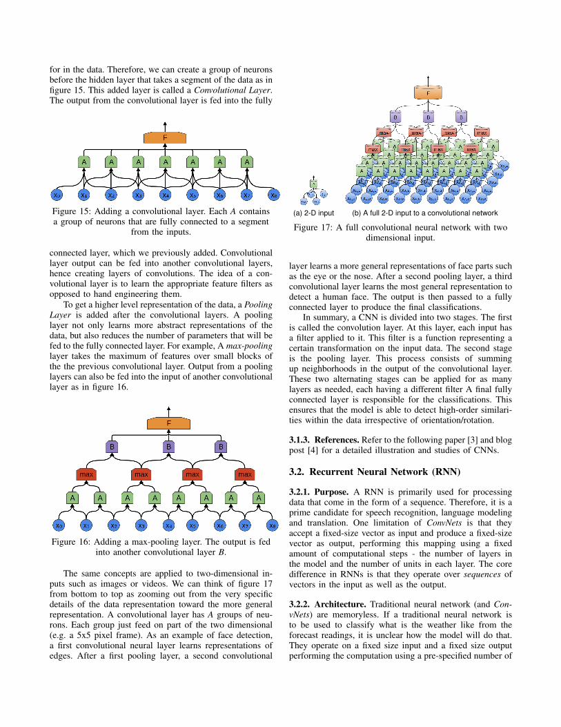
The same concepts are applied to two-dimensional in-puts such as images or videos. We can think of figure 17from bottom to top as zooming out from the very specificdetails of the data representation toward the more generalrepresentation. A convolutional layer has A groups of neu-rons. Each group just feed on part of the two dimensional(e.g. a 5x5 pixel frame). As an example of face detection,a first convolutional neural layer learns representations ofedges. After a first pooling layer, a second convolutional

(a) 2-D input (b) A full 2-D input to a convolutional network

Figure 17: A full convolutional neural network with twodimensional input.

layer learns a more general representations of face parts suchas the eye or the nose. After a second pooling layer, a thirdconvolutional layer learns the most general representation todetect a human face. The output is then passed to a fullyconnected layer to produce the final classifications.

In summary, a CNN is divided into two stages. The firstis called the convolution layer. At this layer, each input hasa filter applied to it. This filter is a function representing acertain transformation on the input data. The second stageis the pooling layer. This process consists of summingup neighborhoods in the output of the convolutional layer.These two alternating stages can be applied for as manylayers as needed, each having a different filter A final fullyconnected layer is responsible for the classifications. Thisensures that the model is able to detect high-order similari-ties within the data irrespective of orientation/rotation.

3.1.3. References. Refer to the following paper [3] and blogpost [4] for a detailed illustration and studies of CNNs.

3.2. Recurrent Neural Network (RNN)

3.2.1. Purpose. A RNN is primarily used for processingdata that come in the form of a sequence. Therefore, it is aprime candidate for speech recognition, language modelingand translation. One limitation of ConvNets is that theyaccept a fixed-size vector as input and produce a fixed-sizevector as output, performing this mapping using a fixedamount of computational steps - the number of layers inthe model and the number of units in each layer. The coredifference in RNNs is that they operate over sequences ofvectors in the input as well as the output.

3.2.2. Architecture. Traditional neural network (and Con-vNets) are memoryless. If a traditional neural network isto be used to classify what is the weather like from theforecast readings, it is unclear how the model will do that.They operate on a fixed size input and a fixed size outputperforming the computation using a pre-specified number of

Figure 18: Recurrent neural network basic component.Left: a chunk of neural network A receives some input x

and outputs a value h. Right: an unrolled RNN.

hidden layers and units. Recurrent neural networks addressthis issue by introducing memory in the network in the formof a loop as in figure 18. You can think of an RNN as a stackof separate neural networks with some parameters of eachnetwork fed from the previous network; these parametersplay the role of a memory.

Inside each repeating module of the recurrent neuralnetwork, the input x at time-step t is concatenated withthe output h at the time-step t-1 and together are passedthrough an activation function to result in the output h at thecurrent time-step t. Figure 19 shows an unrolled illustrationof the this behavior, where the yellow box represents a singleneural network layer with a tanh activation function (otheractivation functions can be used as well).

Figure 19: The repeating module in a RNN with tanh usedas the activation function in the neural network.

Although RNNs are simple in the way that they acceptan input vector x and produce and output vector y, theireffectiveness comes from the fact that the output vector’scontent is influenced not only by the input x, but also bythe entire history of that have been fed to the network inthe past. The RNN has some internal state that gets updatedevery time an input is fed into the network. In the simplestcase, this state is represented as a single hidden vector h.

What happens when there is a long-term dependency?For example, a word in an essay is derived from a wordin the previous paragraph. Unfortunately, the more the gapgrows, RNNs become unable to learn to connect depen-dencies in the sequence. Figure 20 shows the long-termdependency problem in RNNs. Therefore, Long Short TermMemory (LSTM) models have been proposed to overcomethis problem. LSTM are the subject of the next section.

3.2.3. References. Refer to the following paper [5] and blogpost [6] for a detailed illustration and studies of RNNs.

Figure 20: The output h at time t+1 depends on the inputx at times 0 and 1.

3.3. Long Short Term Memory (LSTM)

3.3.1. Purpose. Long Short Term Memory networks areconsidered an improvement to recurrent neural networks thatsolves the problem of long-term dependency. Real-worldimplementations mostly depend on LSTM models ratherthan the basic RNNs.

3.3.2. Architecture. Like RNNs, LSTMs also have a achain-like structure (when unrolled). However, instead ofa single neural network layer in the repeating module as infigure 19, LSTMs have four neural network layers interact-ing in a special harmony as in figure 21.

Figure 21: Four interactive neural network layers insidethe repeating module of LSTM. Each line carries an entire

vector from one node to another.The yellow boxes areneural networks with the indicated activation function. The

pink circles resent point-wise operations like vectoraddition. Lines merging denote concatenation. Lines

forking denote content being cloned to different locations.

The core idea behind LSTMs is the horizontal linepassing through the top of the module. The line representsa cell state that carries information along from one cycleto the next. Addition and multiplication gates control theinformation being stored (or not) in the cell state vector.Each of the four neural network layers is responsible fora specific functionality to be carried out in the cell. Theoperation of cell occurs in three steps as follows:

• First: the first neural network layer from the left (alsocalled forget gate layer) decides what information isgoing to be thrown away from the sate vector. Thesigmoid layer looks at ht−1 and xt, and outputs anumber between 0 and 1 for each number in thecell state vector; that passed through the top line. A

1 represents a ”completely keep this” decision anda 0 represents a ”completely removes this” decision.The output from the first layer is represented as ftbelow:

ft = σ(Wf .[ht−1, xt] + bf )

• Second: the next two layers decide what new in-formation we are going to store in the cell statevector. The sigmoid layer (also called input gatelayer) decides which values will be updated:

it = σ(Wi.[ht−1, xt] + bi)

and the tanh layer creates a vector of new candidatevalues, that could be added to the state:

C̃t = tanh(WC .[ht−1, xt] + bC)

The new cell state vector Ct is computed as follows:

Ct = ft ∗ Ct−1 + ti ∗ C̃t

• Third: the last layer in the cell computes the actualoutput ht. The output value is influenced by the lastsigmoid layer as well as the new cell state vectorthat was just computed.

ot = σ(Wo.[ht−1, x] + bo)

ht = ot ∗ tanh(Ct)

Although what is described so far is a normal LSTM, everypaper involving LSTMs uses a slightly different architecture.A common variation is to let the above functions ft, it andot consider the previous cell state vector Ct; a techniqueknown as peephole connections. Other variations exist de-pending on the training task. Yet, all variations depend onthe idea of the cell state vector that can carry informationfor long time, hence allowing long-term dependencies to betaken in consideration for prediction.

3.3.3. References. Refer to the following papers [7], [8]and generous blog post [9] for a detailed illustration andstudies of LSTMs.

3.4. Restricted Boltzmann Machine (RBM)

3.4.1. Purpose. The first Generative architecture we willexplore is the Restricted Boltzmann Machine. This is notto be confused with the Boltzmann Machine. Figure 22illustrates the difference and the next section will explainthe subtlty. A RBM is commonly utilized in UnsupervisedLearning tasks such as Dimensionality Reduction, FeatureLearning, and Collaborative Filtering.

3.4.2. Architecture. An RBM is composed of two layers,an input layer and a hidden layer. These layers have undi-rected connections between them. The restriction placed ona RBM is that no two nodes in the same layer can have aconnection. This is the differentiator between a BoltzmannMachine and a Restricted Boltzmann Machine. The formerhas existed for many years but it was not until this slight

Figure 22: As you can see, the Boltzmann Machineincludes intra-layer connections whereas the RBM is

limited to only having inter-layer connections.

modification created the latter that this theoretical modelwas utilizable. Without the restriction of having any intra-layer connections, a Boltzmann Machine is completely un-trainable and essentially folds into chaos. We can thereforedefine an RBM formally as a two layer neural networkwith many inter-layer, but no intra-layer connections. Eachconnection bears a weight that is trained during the learningprocedure. By adjusting these weights, an RBM can fit itsparameters(hidden layer nodes) to represent the distributionof the training data. Once this hidden layer is trained, onecan generate samples that fit the distribution of the trainingdata. This technique has been used to compensate for ascarce amount of available data in certain fields.

Figure 23: The architecture of a RBM. The shaded nodesrepresent the visible input layer and the white nodes

represent the hidden layer.

3.4.3. Training. The training procedure for a RBM has afew differentiators over the methods used for Discriminantmodels. While the final step in the procedure entails per-forming stochastic gradient descent to decrease the errorrate, the means by which the error is computed differs. Inan RBM, a procedure called Contrastive Divergence is used.In simplest terms, each iteration can be broken down into3 phases. The hidden layer is created from the input layerbased on probabilities minimizing the free energy of the

model. This will create a hidden layer with certain activa-tions based on that minimization function. This is called thePositive Phase. The next phase is called the Negative Phase.The input layer is the reconstructed based on this hiddenlayer. This newly constructed layer is then propagated backto the hidden layer to create a new set of activations. Thethird phase is the Update phase where the hidden layer inthe Positive phase, and both the reconstructed input andsecond created hidden layer in the Negative phase, are usedto determine the error and update the weights to minimizethis term.

All in all, this learning procedure requires hands-onexperience to master. There are many hyper-parameters suchas the learning rate, momentum, weight-cost, sparsity target,initial values of the weights, number of hidden units, andsize of each batch [10].

For each specific application, a specific set of hyper-parameters must be set. This is the art of training RBM’sand there is no right or wrong way to set them, and onlythrough trial and error can one determine the correct set.

3.4.4. References. Refer to the following papers [11], [12],[13] for a detailed illustration and studies of RBMs.

3.5. Deep Belief Network (DBN)

3.5.1. Purpose. Deep Belief Networks are utilized for learn-ing a representation of some input data. Their purpose isvery similar to the RBM and in practice, researchers rarelyuse RBMs anymore. The DBN can be viewed as the logicalnext step in the timeline of the development of the RBM.It is the next iteration and improvement to this type ofmodel and has been widely accepted as a replacement forthe RBM. Some have argued that since RBM’s have therepresentational power for any function approximation, whatis the use of DBNs? Further research has only been able toconclude that by adding an additional layer, the informationgain must be positive over a more shallow one. This impliesthat there is no harm in adding an additional layer andfrom our understanding, it is to able to detect higher levelabstractions in the data.

3.5.2. Architecture. A Deep Belief Networks is a stack offeedforward RBMs. The output of layer k, which is thehidden layer of an RBM, is the input of the next layer’sRBM. The motivation of this architecture is the idea that anefficient way to learn a complicated model is to combinea set of simpler models that are learned sequentially. Webelieve that by adding layers to the DBN as opposed toadding nodes to the hidden layer of a RBM allows themodel to become more flexible, more representable, andless dependent on the number of nodes in each hidden layer.This requires less manual feature engineering and allows theNeural Net to ”work its magic.” We believe this makes theDBN a more preferable model over the RBM.

3.5.3. Training. The study of training DBNs has filled manyresearch papers and cannot be properly explained to the

Figure 24: This network represents the architecture of aDeep Belief Net. Each pair of layers represents a RBM.As explained, each RBM’s hidden layer is fed into the

input layer of the next RBM.

extent required in the scope of this paper. But more gen-erally, training is performed in a greedy layer-wise fashion.To summarize, all of the learning involved is localized. Byperforming a greedy-layer wise procedure, the network cantrain iteratively and the complexity becomes manageable.This layer-by-layer unsupervised learning algorithm consistsof learning a stack of RBM’s, one RBM at a time, and isillustrated in Figure 25. The first step consists of trainingthe first layer as an RBM that models the input. This firstlayer is used as the input layer for the second layer. Thispart is general modified by choosing only mean activationsor by sampling. This process is repeated for as many layersas desired, each time propagating forward the hidden layerof the previously trained RBM. The parameters(weights)of the model are then updated on this deep architecturewith respect to the log-likelihood. In supervised trainingscenarios, a target output can be substituted for the errorterm instead of the log-likelihood.

3.5.4. References. Refer to the following paper [14] for adetailed illustration and studies of DBNs.

3.6. Deep Boltzmann Machine (DBM)

3.6.1. Purpose. Deep Boltzmann Machines can be views asmulti-layer RBM’s. In contrast to the RBM network beinglimited to one hidden layer, Deep Boltzmann Machines canhave many. This allows the weights to be visible to other lay-ers and forms a more complex version of the RBM. DBM’shave the potential of learning increasingly complex internal

Figure 25: This figure represents the layer-wise trainingprocedure of a Deep Belief Network. Each RBM is

trained, stacked, and their hidden layer is fed to the inputlayer of the next RBM.

representations of the data, which is needed in the fieldsof speech recognition and object assimilation. In practice,however, a DBM is rarely used and often is substituted withthe more promising, and trainable, DBN. We include this ex-planation of the architecture purely as a reference so readerscan differentiate the terms and understand the difference inarchitectures between Deep Boltzmann Machine and DeepBelief Networks.

3.6.2. Architecture. Although very similar to the archi-tecture of a DBN, the architecture of a Deep BoltzmannMachine has one striking difference. Instead of having di-rected connections between each stacked RBM, a DBM hasundirected connections between each layer. This implies thatweights are shared throughout the entire model as opposedto the more layer-wise approach of a DBN. The differenceis illustrated in Figure 26 A DBN is a stacked of connectedRBMs. A Deep Boltzmann Machine is a RBM with multiplehidden layers. This implies a fundamental difference in thetraining procedure. We will not cover the training procedurefor a DBM because it is out of the scope of this literaturesurvey, but bear in mind that it entails factoring in theweights of not just one direction of inputs because signalscan be propagating from both directions of the network.When comparing the two models, DBNs can be viewed asa stack of RBMs whereas the DBM is a hybrid version ofthe RBM.

3.6.3. References. Refer to the following paper [15] for adetailed illustration and studies of DBMs.

3.7. Auto-encoders

3.7.1. Purpose. Auto-encoders are neural networks that aimto learn a compressed representation, or encoding, of theinput data. The model is considered Generative because itis trained to recreate the input data from its hidden layer.Auto-encoders are great for Dimensionality Reduction andare have spawned serious interest recently.

Figure 26: Although each layer is a stacked RBM, thedirection of the connections between layers in Deep Belief

Networks and Deep Boltzmann Machines differ.

3.7.2. Architecture. Auto-encoders have a unique architec-ture. They are designed to have three layers. The first is theinput layer. The third layer is the output layer. This is shownin Figure 27. The middle hidden layer between these two iscalled the Feature layer. The input and output layers of anAuto-encoder are intended to be same after training. Thismiddle layer that serves as an encoder of the input data.This middle layer’s dimensionality can be greater than orless than to the input layer depending on application. In thecase of the feature layer having a dimensionality less thanthe input layer, this model is excellent at performing dimen-sionality reduction. The real focus on these models is theFeature layer that is created during training. Since the inputand output layers will be the same, they are of no interestbesides for training purposes. The middle layer representsan encoding of the data. Architectures such as stacked Auto-Encoders link these Feature Layers in a stacked fashion tocreate higher level abstractions of the data as well. Thismethodology of stacking neural networks to create high levelunderstanding of the data is the key to Deep Learning. Byallowing the network to have more representations, morecorrelations are able to be automatically detected. This iswhy this model is called an Auto-Encoder.

3.7.3. Training. Training can be conceptualized as the net-work trying to ”recreate” the data. The network receivesits inputs and feeds this to the Feature layer. The firstpart of the training process is called the encoding phase.The input data from the first layer is encoded into theFeature layer through adjustable weights. Each node in theFeature layer then propagates a signal forward and, withthe assistance of adjustable weights and biases, maps thisencoded representation back to its original un-encoded state.This is referred to as the decoding phase. To summarize,data is fed into the input layer, encoded in the feature layer,then decoded into the output layer. Error is determined bycomparing this output value to the inputted value, as they

Figure 27: The architecture of a Auto-Encoder. As you cansee, the first and last layers are the same. The middle layerrepresents the Features(encoding) learned during training

should be exactly the same.

3.7.4. References. Refer to the following paper [16] for adetailed illustration and studies of Auto-encoders.

4. Choosing a Model

With the growing number of variations of deep learningmodels, it is important to choose a model that is suitablefor the task in hand. Many factors contribute to choosing amodel that can effectively represent a solution to the task inhand.

• First, study the dataset in hand.• Second, decide whether you want to do a classifica-

tion, a prediction, or learn about data representation.• Third, choose a model and try out different varia-

tions of it until you reach the desired objective.

In table 1, we summarize decision factors for the surveyedmodels in this study. These models cover a wide varietyof domains. Other models fall in one of these generalarchitectures.

5. Applications

At the time we do this extensive survey over deeplearning models, researchers from different labs are utilizingthese approaches in a myriad of real world applications andachieve state of the art performance. In this section, we shedthe light on some of the trending projects being sponsoredby large tech companies.

5.1. Facebook’s DeepFace

Uploading a picture with your friends to Facebook au-tomatically suggests tagging your friends in the picture byrecognizing their faces. Closing the gap to a human-levelperformance in face verification is the main research focusat Facebook’s DeepFace. They derive face representationfrom a nine-layer deep neural network that involves morethan 120 million parameters using several locally connectedlayers without weight sharing. The model was trained ona four million facial images belonging to more than 4000entities, and the result is: the most powerful face recognitionmodule we see in the largest social network in the world!

5.2. Google’s DeepMind

Founded in London in 2010 and acquired by Googlein early 2014, DeepMind algorithms are capable of learningfor themselves directly from raw experience or data, and aregeneral in that they can perform well across a wide varietyof tasks straight out of the box. Their team consists of manyrenowned experts in their respective fields, including but notlimited to deep neural networks, reinforcement learning andsystems neuroscience-inspired models. One recent remark-able achievement is AlphaGo – the first computer programto ever beat a professional player of Go. It was a tremendousmilestone when we have seen a computer brain, powered bydeep learning models, beats a human brain.

create a probabilistic reconstruction of datafeature detectors

5.3. Apple’s Siri

Siri (Speech Interpretation and Recognition Interface)is Apple’s intelligent personal assistant that comes pre-installed with their iPhone devices. Siri’s primary technicalareas focus on a conversational interface, personal contextawareness and service delegation. In the core of the conver-sational interface resides a strong speech recognition engine,powered by deep learning models, that learns a user’s accentand adapts itself to it to respond with better results. Thepower of Siri comes not only from the speech recognitionengine, but also from other machine learning models thatcan carry a full conversation between the user and the devicerelying on a set of web services.

Model CNN RNN LSTM RBM DBN Auto-encoder

Type Discriminative Discriminative Discriminative Generative Generative Generative

Purpose Classification Prediction Prediction Unsupervised Feature Unsupervised Feature Dimensionality

Learning Learning Reduction

Suitable for Processing two- Processing sequence Processing long Learning distributions Creating a probabilistic Creating a compact

dimensional data data sequence data of data reconstruction of data representation of data

Example Images/Videos Language models Language models Generate samples from Trained layer used PCA-like

and Speech and Speech learned hidden representations as feature detectors tasks

TABLE 1: Summary of the surveyed deep learning models

5.4. Microsoft’s Cortana

Analogous to Siri, Cortana is the clever personal as-sistant developed by Microsoft that helps you find thingson your PC, manage your calendar, track packages, findfiles, chat with you, and tell jokes. Cortana learns the userbehavior through a deep learning model in the sense thatthe more you use Cortana, the more personalized your ex-perience will be. Cortana depends heavily on understandinga user’s query and takes actions based on this request. A setof deep learning language models enable setting reminders,making calls, sending emails and answering questions whenrequested by the user. Cortana is a massive improvementin the field of artificial intelligence in human-computerinteraction.

6. Current Research Directions

As demonstrated, deep learning is a vast field [3], [17].Following the theoretical claim that -with enough hiddennodes- a model can be trained to represent any functionor distribution, we are seeing a re-emergence of manyclassical techniques of machine learning, especially with theincreasing improvements in computational resources.

On the discriminant side of models, there is an aggres-sive push towards memory-based models. As shown, onesuccessful model is the LSTM. But in no way is that allthat has been proposed. Memory Networks, Neural TuringNetworks, and Hierarchical Temporal Memory are all similarmemory-based deep neural networks. The advantage of thisdirection is that the networks are able to retain state through-out their lifetimes. The goal of these networks is to enabletasks such as sequence learning and reinforcement learningto be representable and trainable. These tasks require the useof memory to be able to utilize previously seen inputs andcorrelations in future models. In our opinion, reinforcementlearning will be the heavy focus of deep learning in the nextfew years. We are seeing paradigm shift occurring as datascientists are now realizing that deep neural networks can beused as function approximations in reinforcement learningalgorithms. We believe this has a lot of potential and willbe pursuing research in this area in the future.

On the generative side of models, there has been a re-emerging interest in the past few years. Hinton has dropped

a bomb and ignited the entire field of deep learning in hisinfluential paper [14] about a generative architecture. Thefocus then shifted to the more shiny side of unsupervisedlearning. With the explosion of unlabeled data spouting fromthe various sources of big data, the need to improve theseunsupervised deep learning models has been growing. Thefocus on these models varies from being a pre-training stepto be fed forward to a discriminant model to more ”all-in-one” hybrid solutions. There is some past research in thearea of discriminant RBM’s and it’s variations highlightedin Bengio’s paper [18] that we believe will be useful intruly harnessing the representational power of these typicallygenerative models.

7. Conclusion

This concludes our survey of the field of deep learning.To summarize in one statement, we believe deep learningcan be viewed as the art of utilizing deep neural networkstructures to represent any machine learning task. Althoughsome of the theoretical strengths of neural networks has beenclaimed since the 50’s, the recent advancement of computerhardware have made these hypothesis’ verifiable. What weare now seeing a complete redefinition of the tasks that havebeen stapled in the field of machine learning, and the broaderdomain of artificial intelligence.

We view these recent advancements as the beginning ofthe era of truly thinking computers. Whereas old machinelearning techniques such as SVMs, clustering, PCA, ect.are each based on certain statistical characteristics of thedata, neural networks can be viewed as a digital muscle thatcan be strengthen in a certain manner to represent any ofthose models. In our own opinion, old ML techniques can beviewed as discrete learning methods whereas deep learningis more of a continuous learning method. A simple exampleof this is when comparing a stack of linear regressions ontop of each other as opposed to a deep neural network.Ultimately, a stack of linear regressions is still going to belinear no matter what. The equation may have a completelydifferent slope and bias, and be able to represent an arbitraryfunction, but the capabilities are limited. As demonstrated,neural networks are not bound by this linearity. The usageof a nonlinear activation function boosts the representationalpower of certain models so high that there are theoretical

claims that deep learning architectures can be learned to rep-resent any distribution or function [19]. This representationalpower stems from the differentiation of network structuresinto discriminant and generative architectures.

To state that the emergence of the field of deep learninghas correlated with the rise of performance of computerhardware does not illustrate the dependence quite enough.If one thing was clear from our research, it was that thetechniques of deep learning are the most computationallyintensive problems that computers have been introducedto. It is no understatement that deep learning is a fieldthat models its methods based on the world’s most powerprocessor – the human brain. With a strong rooted foun-dation in neuroscience, we have no doubt that the modelsdeveloped by deep learning researchers will aid and pushthe sister field. There is an innate link between the researchneuroscientists are performing on the brain to understandhow the human mind works and the work deep learningexperts are undergoing to emulate this process. We be-lieve that only by the further integration of the fields ofdeep learning and neuroscience, seen in models such asHierarchical Temporal Memory, true general intelligencecan be realized. As such computationally intensive softwaremethods are created, hardware will continue to push theboundaries of what is considered possible.

References

[1] Y. Bengio, “Learning deep architectures for AI,” Foundations andTrends in Machine Learning, vol. 2, no. 1, pp. 1–127, 2009, alsopublished as a book. Now Publishers, 2009.

[2] ——, “Practical recommendations for gradient-based train-ing of deep architectures,” 06 2012. [Online]. Available:http://arxiv.org/abs/1206.5533

[3] I. Arel, D. C. Rose, and T. P. Karnowski, “Deep machine learning -a new frontier in artificial intelligence research [research frontier],”IEEE Computational Intelligence Magazine, vol. 5, no. 4, pp. 13–18,Nov 2010.

[4] O. Christopher, “Conv nets: A modular perspective.”

[5] I. Sutskever, “Training recurrent neural networks,” Ph.D. dissertation,Toronto, Ont., Canada, Canada, 2013, aAINS22066.

[6] K. Andrej, “The unreasonable effectiveness of recurrent neural net-works.”

[7] S. Hochreiter and J. Schmidhuber, “Long short-term memory,”Neural Comput., vol. 9, no. 8, pp. 1735–1780, Nov. 1997. [Online].Available: http://dx.doi.org/10.1162/neco.1997.9.8.1735

[8] K. Greff, R. K. Srivastava, J. Koutnı́k, B. R. Ste-unebrink, and J. Schmidhuber, “LSTM: A search spaceodyssey,” CoRR, vol. abs/1503.04069, 2015. [Online]. Available:http://arxiv.org/abs/1503.04069

[9] O. Christopher, “Understanding lstm networks.”

[10] G. E. Hinton, Neural Networks: Tricks of the Trade: Second Edition.Berlin, Heidelberg: Springer Berlin Heidelberg, 2012, ch. A PracticalGuide to Training Restricted Boltzmann Machines, pp. 599–619.

[11] ——, “Deterministic boltzmann learning performs steepest descent inweight-space,” Neural Comput., vol. 1, no. 1, pp. 143–150, Mar. 1989.[Online]. Available: http://dx.doi.org/10.1162/neco.1989.1.1.143

[12] N. Le Roux and Y. Bengio, “Representational power of restrictedboltzmann machines and deep belief networks,” Neural Comput.,vol. 20, no. 6, pp. 1631–1649, Jun. 2008. [Online]. Available:http://dx.doi.org/10.1162/neco.2008.04-07-510

[13] R. Salakhutdinov and G. Hinton, “Deep Boltzmann machines,” inProceedings of the International Conference on Artificial Intelligenceand Statistics, vol. 5, 2009, pp. 448–455.

[14] G. E. Hinton, S. Osindero, and Y.-W. Teh, “A fastlearning algorithm for deep belief nets,” Neural Comput.,vol. 18, no. 7, pp. 1527–1554, Jul. 2006. [Online]. Available:http://dx.doi.org/10.1162/neco.2006.18.7.1527

[15] R. Salakhutdinov and G. Hinton, “An efficient learning procedurefor deep boltzmann machines,” Neural Comput., vol. 24, no. 8, pp.1967–2006, Aug. 2012.

[16] Y. LeCun, Y. Bengio, and G. Hinton, “Deep learning,” Nature,vol. 521, no. 7553, pp. 436–444, 05 2015. [Online]. Available:http://dx.doi.org/10.1038/nature14539

[17] J. Schmidhuber, “Deep learning in neural networks: An overview,”04 2014. [Online]. Available: http://arxiv.org/abs/1404.7828

[18] H. Larochelle and Y. Bengio, “Classification using discriminativerestricted Boltzmann machines,” in Proceedings of the Twenty-fifthInternational Conference on Machine Learning (ICML’08), W. W.Cohen, A. McCallum, and S. T. Roweis, Eds. ACM, 2008, pp.536–543.

[19] Y. Bengio, A. Courville, and P. Vincent, “Representation learning:A review and new perspectives,” 06 2012. [Online]. Available:http://arxiv.org/abs/1206.5538

[20] W. W. Cohen, A. McCallum, and S. T. Roweis, Eds., Proceedingsof the Twenty-fifth International Conference on Machine Learning(ICML’08). ACM, 2008.

[21] S. Bengio, O. Vinyals, N. Jaitly, and N. Shazeer, “Scheduledsampling for sequence prediction with recurrent neural networks,”06 2015. [Online]. Available: http://arxiv.org/abs/1506.03099

[22] R. Sun, “Introduction to sequence learning,” in SequenceLearning - Paradigms, Algorithms, and Applications. London,UK, UK: Springer-Verlag, 2001, pp. 1–10. [Online]. Available:http://dl.acm.org/citation.cfm?id=647073.713884

[23] J. Snoek, H. Larochelle, and R. P. Adams, “Practical Bayesian Opti-mization of Machine Learning Algorithms,” ArXiv e-prints, Jun. 2012.

[24] S. Rifai, Y. N. Dauphin, P. Vincent, Y. Bengio, and X. Muller,“The manifold tangent classifier,” in Advances in Neural InformationProcessing Systems 24, J. Shawe-Taylor, R. S. Zemel, P. L. Bartlett,F. Pereira, and K. Q. Weinberger, Eds. Curran Associates, Inc., 2011,pp. 2294–2302. [Online]. Available: http://papers.nips.cc/paper/4409-the-manifold-tangent-classifier.pdf

[25] G. E. Hinton, N. Srivastava, A. Krizhevsky, I. Sutskever, andR. Salakhutdinov, “Improving neural networks by preventing co-adaptation of feature detectors,” CoRR, vol. abs/1207.0580, 2012.[Online]. Available: http://arxiv.org/abs/1207.0580

[26] Y. Bengio, Y. Bengio, and S. Bengio, “Modeling high-dimensionaldiscrete data with multi-layer neural networks,” ADVANCES IN NEU-RAL INFORMATION PROCESSING SYSTEMS 12, pp. 400–406,2000.

[27] Y. Lecun, L. Bottou, Y. Bengio, and P. Haffner, “Gradient-basedlearning applied to document recognition,” Proceedings of the IEEE,vol. 86, no. 11, pp. 2278–2324, Nov 1998.