1

Li Deng and Dong Yu Microsoft Research

One Microsoft Way

Redmond, WA 98052

NOW PUBLISHERS, 2014

DEEP LEARNING: METHODS AND APPLICATIONS

2

Table of Contents Chapter 1 Introduction .................................................................................................................... 5

1.1 Definitions and Background............................................................................................. 5

1.2 Organization of This Book ............................................................................................... 8

Chapter 2 Some Historical Context of Deep Learning ................................................................ 11

Chapter 3 Three Classes of Deep Learning Networks ................................................................. 18

3.1 A Three-Way Categorization ......................................................................................... 18

3.2 Deep Networks for Unsupervised or Generative Learning ............................................ 21

3.3 Deep Networks for Supervised Learning ....................................................................... 24

3.4 Hybrid Deep Networks................................................................................................... 26

Chapter 4 Deep Autoencoders --- Unsupervised Learning ........................................................... 29

4.1 Introduction .................................................................................................................... 29

4.2 Use of Deep Autoencoders to Extract Speech Features ................................................. 30

4.3 Stacked Denoising Autoencoders................................................................................... 35

4.4 Transforming Autoencoders ........................................................................................... 35

Chapter 5 Pre-Trained Deep Neural Networks --- A Hybrid ...................................................... 37

5.1 Restricted Boltzmann Machines..................................................................................... 37

5.2 Unsupervised Layer-wise Pretraining ............................................................................ 40

5.3 Interfacing DNNs with HMMs ...................................................................................... 42

Chapter 6 Deep Stacking Networks and Variants --- Supervised Learning ................................ 44

6.1 Introduction .................................................................................................................... 44

6.2 A Basic Architecture of the Deep Stacking Network .................................................... 45

6.3 A Method for Learning the DSN Weights ..................................................................... 46

6.4 The Tensor Deep Stacking Network .............................................................................. 48

6.5 The Kernelized Deep Stacking Network ........................................................................ 50

Chapter 7 Selected Applications in Speech and Audio Processing ............................................. 53

7.1 Acoustic Modeling for Speech Recognition................................................................... 53

7.1.1 Back to primitive spectral features of speech................................................................. 54

7.1.2 The DNN-HMM architecture vs. use of DNN-derived features .................................... 56

7.1.3 Noise robustness by deep learning ................................................................................. 59

7.1.4 Output representations in the DNN ................................................................................ 60

7.1.5 Adaptation of the DNN-based speech recognizers ........................................................ 62

7.1.6 Better architectures and nonlinear units ......................................................................... 63

7.1.7 Better optimization and regularization …………………………………………………67

7.2 Speech Synthesis ............................................................................................................ 70

3

7.3 Audio and Music Processing .......................................................................................... 71

Chapter 8 Selected Applications in Language Modeling and Natural Language Processing ...... 73

8.1 Language Modeling........................................................................................................ 73

8.2 Natural Language Processing ......................................................................................... 77

Chapter 9 Selected Applications in Information Retrieval .......................................................... 84

9.1 A Brief Introduction to Information Retrieval ............................................................... 84

9.2 Semantic Hashing with Deep Autoencoders for Document Indexing and Retrieval ..... 85

9.3 Deep-Structured Semantic Modeling for Document Retrieval ...................................... 86

9.4 Use of Deep Stacking Networks for Information Retrieval ........................................... 91

Chapter 10 Selected Applications in Object Recognition and Computer Vision ........................ 92

10.1 Unsupervised or Generative Feature Learning............................................................... 92

10.2 Supervised Feature Learning and Classification ............................................................ 94

Chapter 11 Selected Applications in Multi-modal and Multi-task Learning ............................. 101

11.1 Multi-Modalities: Text and Image ............................................................................... 101

11.2 Multi-Modalities: Speech and Image ........................................................................... 104

11.3 Multi-Task Learning within the Speech, NLP or Image Domain ................................ 106

Chapter 12 Epilogues ................................................................................................................. 110

BIBLIOGRAPHY ....................................................................................................................... 114

4

Abstract

This book is aimed to provide an overview of general deep learning methodology and its

applications to a variety of signal and information processing tasks. The application areas are

chosen with the following three criteria: 1) expertise or knowledge of the authors; 2) the

application areas that have already been transformed by the successful use of deep learning

technology, such as speech recognition and computer vision; and 3) the application areas that have

the potential to be impacted significantly by deep learning and that have gained concentrated

research efforts, including natural language and text processing, information retrieval, and

multimodal information processing empowered by multi-task deep learning.

In Chapter 1, we provide the background of deep learning, as intrinsically connected to the use of

multiple layers of nonlinear transformations to derive features from the sensory signals such as

speech and visual images. In the most recent literature, deep learning is embodied also as

representation learning, which involves a hierarchy of features or concepts where higher-level

representations of them are defined from lower-level ones and where the same lower-level

representations help to define higher-level ones. In Chapter 2, a brief historical account of deep

learning is presented. In particular, selected chronological development of speech recognition is

used to illustrate the recent impact of deep learning that has become a dominant technology in

speech recognition industry within only a few years since the start of a collaboration between

academic and industrial researchers in applying deep learning to speech recognition. In Chapter 3,

a three-way classification scheme for a large body of work in deep learning is developed. We

classify a growing number of deep learning techniques into unsupervised, supervised, and hybrid

categories, and present qualitative descriptions and a literature survey for each category. From

Chapter 4 to Chapter 6, we discuss in detail three popular deep networks and related learning

methods, one in each category. Chapter 4 is devoted to deep autoencoders as a prominent example

of the unsupervised deep learning techniques. Chapter 5 gives a major example in the hybrid deep

network category, which is the discriminative feed-forward neural network for supervised learning

with many layers initialized using layer-by-layer generative, unsupervised pre-training. In Chapter

6, deep stacking networks and several of the variants are discussed in detail, which exemplify the

discriminative or supervised deep learning techniques in the three-way categorization scheme.

In Chapters 7-11, we select a set of typical and successful applications of deep learning in diverse

areas of signal and information processing and of applied artificial intelligence. In Chapter 7, we

review the applications of deep learning to speech and audio processing, with emphasis on speech

recognition organized according to several prominent themes. In Chapters 8, we present recent

results of applying deep learning to language modeling and natural language processing. Chapter

9 is devoted to selected applications of deep learning to information retrieval including Web search.

In Chapter 10, we cover selected applications of deep learning to image object recognition in

computer vision. Selected applications of deep learning to multi-modal processing and multi-task

learning are reviewed in Chapter 11. Finally, an epilogue is given in Chapter 12 to summarize

what we presented in earlier chapters and to discuss future challenges and directions.

5

CHAPTER 1

INTRODUCTION

1.1 Definitions and Background

Since 2006, deep structured learning, or more commonly called deep learning or hierarchical

learning, has emerged as a new area of machine learning research (Hinton et al., 2006; Bengio,

2009). During the past several years, the techniques developed from deep learning research have

already been impacting a wide range of signal and information processing work within the

traditional and the new, widened scopes including key aspects of machine learning and artificial

intelligence; see overview articles in (Bengio, 2009; Arel et al., 2010; Yu and Deng, 2011; Deng,

2011, 2013; Hinton et al., 2012; Bengio et al., 2013a), and also the media coverage of this progress

in (Markoff, 2012; Anthes, 2013). A series of workshops, tutorials, and special issues or

conference special sessions in recent years have been devoted exclusively to deep learning and its

applications to various signal and information processing areas. These include:

2008 NIPS Deep Learning Workshop;

2009 NIPS Workshop on Deep Learning for Speech Recognition and Related Applications;

2009 ICML Workshop on Learning Feature Hierarchies;

2011 ICML Workshop on Learning Architectures, Representations, and Optimization for

Speech and Visual Information Processing;

2012 ICASSP Tutorial on Deep Learning for Signal and Information Processing;

2012 ICML Workshop on Representation Learning;

2012 Special Section on Deep Learning for Speech and Language Processing in IEEE

Transactions on Audio, Speech, and Language Processing (T-ASLP, January);

2010, 2011, and 2012 NIPS Workshops on Deep Learning and Unsupervised Feature

Learning;

2013 NIPS Workshops on Deep Learning and on Output Representation Learning;

6

2013 Special Issue on Learning Deep Architectures in IEEE Transactions on Pattern

Analysis and Machine Intelligence (T-PAMI, September).

2013 International Conference on Learning Representations;

2013 ICML Workshop on Representation Learning Challenges;

2013 ICML Workshop on Deep Learning for Audio, Speech, and Language Processing;

2013 ICASSP Special Session on New Types of Deep Neural Network Learning for Speech

Recognition and Related Applications.

The authors have been actively involved in deep learning research and in organizing or providing

several of the above events, tutorials, and editorials. In particular, they gave tutorials and invited

lectures on this topic at various places. Part of this book is based on their tutorials and lecture

material.

Before embarking on describing details of deep learning, let’s provide necessary definitions. Deep

learning has various closely related definitions or high-level descriptions:

Definition 1: A class of machine learning techniques that exploit many layers of non-linear

information processing for supervised or unsupervised feature extraction and transformation,

and for pattern analysis and classification.

Definition 2: “A sub-field within machine learning that is based on algorithms for learning

multiple levels of representation in order to model complex relationships among data.

Higher-level features and concepts are thus defined in terms of lower-level ones, and such a

hierarchy of features is called a deep architecture. Most of these models are based on

unsupervised learning of representations.” (Wikipedia on “Deep Learning” around March

2012.)

Definition 3: “A sub-field of machine learning that is based on learning several levels of

representations, corresponding to a hierarchy of features or factors or concepts, where higher-

level concepts are defined from lower-level ones, and the same lower-level concepts can help

to define many higher-level concepts. Deep learning is part of a broader family of machine

learning methods based on learning representations. An observation (e.g., an image) can be

represented in many ways (e.g., a vector of pixels), but some representations make it easier

to learn tasks of interest (e.g., is this the image of a human face?) from examples, and research

in this area attempts to define what makes better representations and how to learn them.”

(Wikipedia on “Deep Learning” around February 2013.)

Definition 4: “Deep learning is a set of algorithms in machine learning that attempt to learn

in multiple levels, corresponding to different levels of abstraction. It typically uses artificial

7

neural networks. The levels in these learned statistical models correspond to distinct levels

of concepts, where higher-level concepts are defined from lower-level ones, and the same

lower-level concepts can help to define many higher-level concepts.” See Wikipedia

http://en.wikipedia.org/wiki/Deep_learning on “Deep Learning” as of this most recent update

in October 2013.

Definition 5: “Deep Learning is a new area of Machine Learning research, which has been

introduced with the objective of moving Machine Learning closer to one of its original goals:

Artificial Intelligence. Deep Learning is about learning multiple levels of representation and

abstraction that help to make sense of data such as images, sound, and text.” See

https://github.com/lisa-lab/DeepLearningTutorials

Note that the deep learning that we discuss in this book is about learning in deep architectures for

signal and information processing. It is not about deep understanding of the signal or information,

although in many cases they may be related. It should also be distinguished from the overloaded

term in educational psychology: “Deep learning describes an approach to learning that is

characterized by active engagement, intrinsic motivation, and a personal search for meaning.”

http://www.blackwellreference.com/public/tocnode?id=g9781405161251_chunk_g97814051612

516_ss1-1

Common among the various high-level descriptions of deep learning above are two key aspects:

1) models consisting of multiple layers or stages of nonlinear information processing; and 2)

methods for supervised or unsupervised learning of feature representation at successively higher,

more abstract layers. Deep learning is in the intersections among the research areas of neural

networks, artificial intelligence, graphical modeling, optimization, pattern recognition, and signal

processing. Three important reasons for the popularity of deep learning today are the drastically

increased chip processing abilities (e.g., general-purpose graphical processing units or GPGPUs),

the significantly lowered cost of computing hardware, and the recent advances in machine learning

and signal/information processing research. These advances have enabled the deep learning

methods to effectively exploit complex, compositional nonlinear functions, to learn distributed and

hierarchical feature representations, and to make effective use of both labeled and unlabeled data.

Active researchers in this area include those at University of Toronto, New York University,

University of Montreal, Stanford University, Microsoft Research (since 2009), Google (since

about 2011), IBM Research (since about 2011), Baidu (since 2012), Facebook (since 2013), UC-

Berkeley, UC-Irvine, IDIAP, IDSIA, University College London, University of Michigan,

Massachusetts Institute of Technology, University of Washington, and numerous other places; see

http://deeplearning.net/deep-learning-research-groups-and-labs/ for a more detailed list. These

researchers have demonstrated empirical successes of deep learning in diverse applications of

computer vision, phonetic recognition, voice search, conversational speech recognition, speech

and image feature coding, semantic utterance classification, natural language understanding, hand-

writing recognition, audio processing, information retrieval, robotics, and even in the analysis of

molecules that may lead to discovery of new drugs as reported recently by Markoff (2012).

8

In addition to the reference list provided at the end of this book, which may be outdated not long

after the publication of this book, there are a number of excellent and frequently updated reading

lists, tutorials, software, and video lectures online at:

http://deeplearning.net/reading-list/

http://ufldl.stanford.edu/wiki/index.php/UFLDL_Recommended_Readings

http://www.cs.toronto.edu/~hinton/

http://deeplearning.net/tutorial/

http://ufldl.stanford.edu/wiki/index.php/UFLDL_Tutorial

1.2 Organization of This Book

The rest of the book is organized as follows:

In Chapter 2, we provide a brief historical account of deep learning, mainly from the perspective

of how speech recognition technology has been hugely impacted by deep learning, and how the

revolution got started and has gained and sustained immense momentum.

In Chapter 3, a three-way categorization scheme for a majority of the work in deep learning is

developed. They include unsupervised, supervised, and hybrid deep learning networks, where in

the latter category unsupervised learning (or pre-training) is exploited to assist the subsequent stage

of supervised learning when the final tasks pertain to classification. The supervised and hybrid

deep networks often have the same type of architectures or the structures in the deep networks, but

the unsupervised deep networks tend to have different architectures from the others.

Chapters 4-6 are devoted, respectively, to three popular types of deep architectures, one from each

of the classes in the three-way categorization scheme reviewed in Chapter 3. In Chapter 4, we

discuss in detail deep autoencoders as a prominent example of the unsupervised deep learning

networks. No class labels are used in the learning, although supervised learning methods such as

back-propagation are cleverly exploited when the input signal itself, instead of any label

information of interest to possible classification tasks, is treated as the “supervised” signal.

In Chapter 5, as a major example in the hybrid deep network category, we present in detail the

deep neural networks with unsupervised and largely generative pre-training to boost the

effectiveness of supervised training. This benefit is found critical when the training data are limited

and no other appropriate regularization ways (i.e., dropout) are exploited. The particular pre-

9

training method based on restricted Boltzmann machines and the related deep belief networks

described in this chapter has been historically significant as it ignited the intense interest in the

early applications of deep learning to speech recognition and other information processing tasks.

In addition to this retrospective review, subsequent development and different paths from the more

recent perspective are discussed.

In Chapter 6, the basic deep stacking networks and their several extensions are discussed in detail,

which exemplify the discriminative, supervised deep learning networks in the three-way

classification scheme. This group of deep networks operate in many ways that are distinct from

the deep neural networks. Most notably, they use target labels in constructing each of many layers

or modules in the overall deep networks. Assumptions made about part of the networks, such as

linear output units in each of the modules, simplify the learning algorithms and enable a much

wider variety of network architectures to be constructed and learned than the networks discussed

in Chapters 4 and 5.

In Chapters 7-11, we select a set of typical and successful applications of deep learning in diverse

areas of signal and information processing. In Chapter 7, we review the applications of deep

learning to speech recognition, speech synthesis, and audio processing. Subsections surrounding

the main subject of speech recognition are created based on several prominent themes on the topic

in the literature.

In Chapters 8, we present recent results of applying deep learning to language modeling and natural

language processing, where we highlight the key recent development in embedding symbolic

entities such as words into low-dimensional, continuous-valued vectors.

Chapter 9 is devoted to selected applications of deep learning to information retrieval including

web search.

In Chapter 10, we cover selected applications of deep learning to image object recognition in

computer vision. The chapter is divided to two main classes of deep learning approaches: 1)

unsupervised feature learning, and 2) supervised learning for end-to-end and joint feature learning

and classification.

Selected applications to multi-modal processing and multi-task learning are reviewed in Chapter

11, divided into three categories according to the nature of the multi-modal data as inputs to the

deep learning systems. For single-modality data of speech, text, or image, a number of recent

multi-task learning studies based on deep learning methods are reviewed in the literature.

Finally, an epilogue is given in Chapter 12 to summarize the book and to discuss future challenges

and directions.

This short monograph contains the material expanded from two tutorials that the authors gave, one

at APSIPA in October 2011 and the other at ICASSP in March 2012. Substantial updates have

been made based on the literature up to January 2014 (including the materials presented at NIPS-

10

2013 and at IEEE-ASRU-2013 both held in December of 2013), focusing on practical aspects in

the fast development of deep learning research and technology during the interim years.

11

CHAPTER 2

SOME HISTORICAL CONTEXT OF DEEP

LEARNING

Until recently, most machine learning and signal processing techniques had exploited shallow-

structured architectures. These architectures typically contain at most one or two layers of

nonlinear feature transformations. Examples of the shallow architectures are Gaussian mixture

models (GMMs), linear or nonlinear dynamical systems, conditional random fields (CRFs),

maximum entropy (MaxEnt) models, support vector machines (SVMs), logistic regression, kernel

regression, multi-layer perceptrons (MLPs) with a single hidden layer including extreme learning

machines (ELMs). For instance, SVMs use a shallow linear pattern separation model with one or

zero feature transformation layer when the kernel trick is used or otherwise. (Notable exceptions

are the recent kernel methods that have been inspired by and integrated with deep learning; e.g.

Cho and Saul, 2009; Deng et al., 2012; Vinyals et al., 2012; Aslan et al., 2013). Shallow

architectures have been shown effective in solving many simple or well-constrained problems, but

their limited modeling and representational power can cause difficulties when dealing with more

complicated real-world applications involving natural signals such as human speech, natural sound

and language, and natural image and visual scenes.

Human information processing mechanisms (e.g., vision and audition), however, suggest the need

of deep architectures for extracting complex structure and building internal representation from

rich sensory inputs. For example, human speech production and perception systems are both

equipped with clearly layered hierarchical structures in transforming the information from the

waveform level to the linguistic level (Baker et al., 2009, 2009a; Deng, 1999, 2003). In a similar

vein, the human visual system is also hierarchical in nature, mostly in the perception side but

interestingly also in the “generation” side (George, 2008; Bouvrie, 2009; Poggio, 2007). It is

natural to believe that the state-of-the-art can be advanced in processing these types of natural

signals if efficient and effective deep learning algorithms can be developed.

Historically, the concept of deep learning originated from artificial neural network research.

(Hence, one may occasionally hear the discussion of “new-generation neural networks”.) Feed-

forward neural networks or MLPs with many hidden layers, which are often referred to as deep

neural networks (DNNs), are good examples of the models with a deep architecture. Back-

propagation (BP), popularized in 1980’s, has been a well-known algorithm for learning the

parameters of these networks. Unfortunately back-propagation alone did not work well in practice

then for learning networks with more than a small number of hidden layers (see a review and

analysis in (Bengio, 2009; Glorot and Bengio, 2010). The pervasive presence of local optima and

other optimization challenges in the non-convex objective function of the deep networks are the

main source of difficulties in the learning. Back-propagation is based on local gradient information,

and starts usually at some random initial points. It often gets trapped in poor local optima when

the batch-mode or even stochastic gradient descent BP algorithm is used. The severity increases

12

significantly as the depth of the networks increases. This difficulty is partially responsible for

steering away most of the machine learning and signal processing research from neural networks

to shallow models that have convex loss functions (e.g., SVMs, CRFs, and MaxEnt models), for

which the global optimum can be efficiently obtained at the cost of reduced modeling power,

although there had been continuing work on neural networks with limited scale and impact (e.g.,

Hochreiter and Schmidhuber, 1997; LeCun et al., 1998; Bourlard and Morgan, 1993; Deng et al.,

1994s; Bridle et al., 1998; Robinson, 1994; Morgan, et al., 2005).

The optimization difficulty associated with the deep models was empirically alleviated when a

reasonably efficient, unsupervised learning algorithm was introduced in the two seminar papers

(Hinton et al., 2006; Hinton and Salakhutdinov, 2006). In these papers, a class of deep generative

models, called deep belief network (DBN), was introduced. A DBN is composed of a stack of

restricted Boltzmann machines (RBMs). A core component of the DBN is a greedy, layer-by-layer

learning algorithm which optimizes DBN weights at time complexity linear to the size and depth

of the networks. Separately and with some surprise, initializing the weights of an MLP with a

correspondingly configured DBN often produces much better results than that with the random

weights. As such, MLPs with many hidden layers, or deep neural networks (DNN), which are

learned with unsupervised DBN pre-training followed by back-propagation fine-tuning is

sometimes also called DBNs in the literature (e.g., Dahl et al., 2011; Mohamed et al., 2010, 2012).

More recently, researchers have been more careful in distinguishing DNNs from DBNs (Dahl et

al., 2012; Hinton et al., 2012), and when DBN is used to initialize the training of a DNN, the

resulting network is sometimes called the DBN-DNN (Hinton et al., 2012).

Independently of the RBM development, in 2006 two alternative, non-probabilistic, non-

generative, unsupervised deep models were published. One is an autoencoder variant with greedy

layer-wise training much like the DBN training (Bengio et al., 2006). Another is an energy-based

model with unsupervised learning of sparse over-complete representations (Ranzato et al., 2006).

They both can be effectively used to pre-train a deep neural network, much like the DBN.

In addition to the supply of good initialization points, the DBN comes with additional attractive

properties. First, the learning algorithm makes effective use of unlabeled data. Second, it can be

interpreted as Bayesian probabilistic generative model. Third, the over-fitting problem, which is

often observed in the models with millions of parameters such as DBNs, and the under-fitting

problem, which occurs often in deep networks, can be effectively addressed by the generative pre-

training step. An insightful analysis on what speech information DBNs can capture is provided in

(Mohamed et al. 2012a).

Using hidden layers with many neurons in a DNN significantly improves the modeling power of

the DNN and creates many closely optimal configurations. Even if parameter learning is trapped

into a local optimum, the resulting DNN can still perform quite well since the chance of having a

poor local optimum is lower than when a small number of neurons are used in the network. Using

deep and wide neural networks, however, would cast great demand to the computational power

during the training process and this is one of the reasons why it is not until recent years that

researchers have started exploring both deep and wide neural networks in a serious manner.

13

Better learning algorithms and different nonlinearities also contributed to the success of DNNs.

Stochastic gradient descend (SGD) algorithms are the most efficient algorithm when the training

set is large and redundant as is the case for most applications (Bottou and LeCun, 2004). Recently,

SGD is shown to be effective for parallelizing over many machines with an asynchronous mode

(Dean et al., 2012) or over multiple GPUs through pipelined BP (Chen et al., 2012). Further, SGD

can often allow the training to jump out of local optima due to the noisy gradients estimated from

a single or a small batch of samples. Other learning algorithms such as Hessian free (Martens 2010,

Kingsbury et al., 2012) or Krylov subspace methods (Vinyals and Povey, 2011) have shown a

similar ability.

For the highly non-convex optimization problem of DNN learning, it is obvious that better

parameter initialization techniques will lead to better models since optimization starts from these

initial models. What was not obvious, however, is how to efficiently and effectively initialize DNN

parameters and how the use of very large amounts of training data can alleviate the learning

problem until more recently (Hinton et al. 2006; Hinton and Salakhutdinov, 2006; Bengio, 2009;

Vincent et al., 2010; Deng et al., 2010; Yu et al., 2010c; Dahl et al., 2010, 2012; Seide et al. 2011;

Hinton et al., 2012). The DNN parameter initialization technique that attracted the most attention

is the unsupervised pretraining technique proposed in (Hinton et al. 2006; Hinton and

Salakhutdinov, 2006) discussed earlier.

The DBN pretraining procedure is not the only one that allows effective initialization of DNNs.

An alternative unsupervised approach that performs equally well is to pretrain DNNs layer by layer

by considering each pair of layers as a de-noising autoencoder regularized by setting a random

subset of the input nodes to zero (Bengio, 2009; Vincent et al., 2010). Another alternative is to use

contractive autoencoders for the same purpose by favoring representations that are more robust to

the input variations, i.e., penalizing the gradient of the activities of the hidden units with respect

to the inputs (Rifai et al., 2011). Further, Ranzato et al. (2007) developed the Sparse Encoding

Symmetric Machine (SESM), which has a very similar architecture to RBMs as building blocks

of a DBN. The SESM may also be used to effectively initialize the DNN training. In addition to

unsupervised pretraining using greedy layer-wise procedures (Hinton and Salakhutdinov, 2006;

Bengio et al., 2006; Ranzato et al., 2007), the supervised pretraining, or sometimes called

discriminative pretraining, has also been shown to be effective (Seide et al., 2011; Yu et al., 2011;

Hinton et al., 2012) and in cases where labeled training data are abundant performs better than the

unsupervised pretraining techniques. The idea of the discriminative pretraining is to start from a

one-hidden-layer MLP trained with the BP algorithm. Every time when we want to add a new

hidden layer we replace the output layer with a randomly initialized new hidden and output layer

and train the whole new MLP (or DNN) using the BP algorithm. Different from the unsupervised

pretraining techniques, the discriminative pretraining technique requires labels.

Researchers who apply deep learning to speech and vision analyzed what DNNs capture in speech

and images. For example, Mohamed et al. (2012a) applied a dimensionality reduction method to

visualize the relationship among the feature vectors learned by the DNN. They found that the

DNN’s hidden activity vectors preserve the similarity structure of the feature vectors at multiple

scales, and that this is especially true for the filterbank features. A more elaborated visualization

method, based on a top-down generative process in the reverse direction of the classification

network, was recently developed by Zeiler and Fergus (2013) for examining what features the deep

14

convolutional networks capture from the image data. The power of the deep networks is shown to

be their ability to extract appropriate features and do discrimination jointly (LeCun, 2012).

As another way to concisely introduce the DNN, we can review the history of artificial neural

networks using a “Hype Cycle”, which is a graphic representation of the maturity, adoption and

social application of specific technologies. The 2012 version of the Hype Cycles graph compiled

by Gartner is shown in Figure 2.1. It intends to show how a technology or application will evolve

over time (according to five phases: technology trigger, peak of inflated expectations, trough of

disillusionment, slope of enlightenment, and plateau of production), and to provide a source of

insight to manage its deployment.

Figure 2.1. Gartner Hyper Cycle graph representing five phases of a technology

(http://en.wikipedia.org/wiki/Hype_cycle)

Applying the Gartner Hyper Cycle to the artificial neural network development, we created Figure

2.2 to align different generations of the neural network with the various phases designated in the

Hype Cycle. The peak activities (“expectations” or “media hype” on the vertical axis) occurred in

late 1980’s and early 1990’s, corresponding to the height of what is often referred to as the “second

generation” of neural networks. The deep belief network (DBN) and a fast algorithm for training

it were invented in 2006 (Hinton and Salakhudinov, 2006; Hinton et al., 2006). When the DBN

was used to initialize the DNN, the learning became highly effective and this has inspired the

subsequent fast growing research (“enlightenment” phase shown in Figure 2.2). Applications of

the DBN and DNN to industry-scale speech feature extraction and speech recognition started in

2009 when leading academic and industrial researchers with both deep learning and speech

expertise collaborated; see reviews in (Hinton et al., 2012; Deng et al., 2013b). This collaboration

fast expanded the work of speech recognition using deep learning methods to increasingly larger

successes (Yu et al., 2010c; Seide et al., 2011; Hinton et al., 2012; Deng et al., 2013a), many of

which will be covered in the remainder of this book. The height of the “plateau of productivity”

phase, not yet reached in our opinion, is expected to be higher than in the stereotypical curve

(circled with a question mark in Figure 2.2), and is marked by the dashed line that moves straight

up.

15

Figure 2.2: Applying Gartner Hyper Cycle graph to analyzing the history of artificial neural

network technology (We thank our colleague John Platt during 2012 for bringing this type of

“Hyper Cycle” graph to our attention for concisely analyzing the neural network history).

We show in Figure 2.3 the history of speech recognition, which has been compiled by NIST,

organized by plotting the word error rate (WER) as a function of time for a number of increasingly

difficult speech recognition tasks. Note all WER results were obtained using the GMM-HMM

technology. When one particularly difficult task (Switchboard) is extracted from Figure 2.3, we

see a flat curve over many years using the GMM-HMM technology but after the DNN technology

is used the WER drops sharply (marked by the red star in Figure 2.4).

16

Figure 2.3: The famous NIST plot showing the historical speech recognition error rates achieved

by the GMM-HMM approach for a number of increasingly difficult speech recognition tasks. Data

source: http://itl.nist.gov/iad/mig/publications/ASRhistory/index.html

Figure 2.4. Extracting WERs of one task from Figure 2.3 and adding the significantly lower WER

(marked by the star) achieved by the DNN technology approach.

17

In the next Chapter, an overview is provided on the various architectures of deep learning, followed

by more detailed expositions of a few widely studied architectures and methods and by selected

applications in signal and information processing including speech and audio, natural language,

information retrieval, vision, and multi-modal processing.

18

CHAPTER 3

THREE CLASSES OF DEEP LEARNING

NETWORKS

3.1 A Three-Way Categorization

As described earlier, deep learning refers to a rather wide class of machine learning techniques

and architectures, with the hallmark of using many layers of non-linear information processing

that are hierarchical in nature. Depending on how the architectures and techniques are intended for

use, e.g., synthesis/generation or recognition/classification, one can broadly categorize most of the

work in this area into three major classes:

1) Deep networks for unsupervised or generative learning, which are intended to capture

high-order correlation of the observed or visible data for pattern analysis or synthesis

purposes when no information about target class labels is available. Unsupervised feature

or representation learning in the literature refers to this category of the deep networks.

When used in the generative mode, may also be intended to characterize joint statistical

distributions of the visible data and their associated classes when available and being

treated as part of the visible data. In the latter case, the use of Bayes rule can turn this type

of generative networks into a discriminative one for learning.

2) Deep networks for supervised learning, which are intended to directly provide

discriminative power for pattern classification purposes, often by characterizing the

posterior distributions of classes conditioned on the visible data. Target label data are

always available in direct or indirect forms for such supervised learning. They are also

called discriminative deep networks.

3) Hybrid deep networks, where the goal is discrimination which is assisted, often in a

significant way, with the outcomes of generative or unsupervised deep networks. This can

be accomplished by better optimization or/and regularization of the deep networks in

category 2). The goal can also be accomplished when discriminative criteria for supervised

learning are used to estimate the parameters in any of the deep generative or unsupervised

deep networks in category 1) above.

Note the use of “hybrid” in 3) above is different from that used sometimes in the literature, which

refers to the hybrid systems for speech recognition feeding the output probabilities of a neural

network into an HMM (Bengio, 1991; Bengio et al., 1992; Bourlard and Morgan, 1993; Morgan,

2012).

19

By the commonly adopted machine learning tradition (e.g., Chapter 28 in Murphy, 2012; Deng

and Li, 2013), it may be natural to just classify deep learning techniques into deep discriminative

models (e.g., deep neural networks or DNNs, recurrent neural networks or RNNs, convolutional

neural networks or CNNs, etc.) and generative/unsupervised models (e.g., restricted Boltzmann

machine or RBMs, deep belief networks or DBNs, deep Boltzmann machines (DBMs), regularized

autoencoders, etc.). This two-way classification scheme, however, misses a key insight gained in

deep learning research about how generative or unsupervised-learning models can greatly improve

the training of DNNs and other deep discriminative or supervised-learning models via better

regularization or optimization. Also, deep networks for unsupervised learning may not necessarily

need to be probabilistic or be able to meaningfully sample from the model (e.g., traditional

autoencoders, sparse coding networks, etc.). We note here that more recent studies have

generalized the traditional denoising autoencoders so that they can be efficiently sampled from

and thus have become generative models (Alain and Bengio, 2013; Bengio et al., 2013, 2013b).

Nevertheless, the traditional two-way classification indeed points to several key differences

between deep networks for unsupervised and supervised learning. Compared between the two,

deep supervised-learning models such as DNNs are usually more efficient to train and test, more

flexible to construct, and more suitable for end-to-end learning of complex systems (e.g., no

approximate inference and learning such as loopy belief propagation). On the other hand, the deep

unsupervised-learning models, especially the probabilistic generative ones, are easier to interpret,

easier to embed domain knowledge, easier to compose, and easier to handle uncertainty, but they

are typically intractable in inference and learning for complex systems. These distinctions are

retained also in the proposed three-way classification which is hence adopted throughout this book.

Below we review representative work in each of the above three categories, where several basic

definitions are summarized in Table 3.1. Applications of these deep architectures, with varied ways

of learning including supervised, unsupervised, or hybrid, are deferred to Chapters 7-11.

20

TABLE 3.1. BASIC DEEP LEARNING TERMINOLOGIES

Deep Learning: a class of machine learning techniques, where many layers of information

processing stages in hierarchical architectures are exploited for unsupervised feature learning and

for pattern analysis/classification. The essence of deep learning is to compute hierarchical

features or representations of the observational data, where the higher-level features or factors

are defined from lower-level ones. The family of deep learning methods have been growing

increasingly richer, encompassing those of neural networks, hierarchical probabilistic models,

and a variety of unsupervised and supervised feature learning algorithms.

Deep belief network (DBN): probabilistic generative models composed of multiple layers of

stochastic, hidden variables. The top two layers have undirected, symmetric connections between

them. The lower layers receive top-down, directed connections from the layer above.

Boltzmann machine (BM): a network of symmetrically connected, neuron-like units that make

stochastic decisions about whether to be on or off.

Restricted Boltzmann machine (RBM): a special type of BM consisting of a layer of visible

units and a layer of hidden units with no visible-visible or hidden-hidden connections.

Deep neural network (DNN): a multilayer perceptron with many hidden layers, whose weights

are fully connected and are often initialized using either an unsupervised or a supervised

pretraining technique. (In the literature prior to 2012, a DBN was often used incorrectly to mean

a DNN.)

Deep autoencoder: a “discriminative” DNN whose output targets are the data input itself rather

than class labels; hence an unsupervised learning model. When trained with a denoising criterion,

a deep autoencoder is also a generative model and can be sampled from.

Distributed representation: an internal representation of the observed data in such a way that

they are modeled as being explained by the interactions of many hidden factors. A particular

factor learned from configurations of other factors can often generalize well to new

configurations. Distributed representations naturally occur in a “connectionist” neural network,

where a concept is represented by a pattern of activity across a number of many units and where

at the same time a unit typically contributes to many concepts. One key advantage of such many-

to-many correspondence is that they provide robustness in representing the internal structure of

the data in terms of graceful degradation and damage resistance. Another key advantage is that

they facilitate generalizations of concepts and relations, thus enabling reasoning abilities.

21

3.2 Deep Networks for Unsupervised or Generative

Learning

Unsupervised learning refers to no use of task specific supervision information (e.g., target class

labels) in the learning process. Many deep networks in this category can be used to meaningfully

generate samples by sampling from the networks, with examples of RBMs, DBNs, DBMs, and

generalized denoising autoencoders (Bengio et al., 2013), and are thus generative models. Some

networks in this category, however, cannot be easily sampled, with examples of sparse coding

networks and the original forms of deep autoencoders, and are thus not generative in nature.

Among the various subclasses of generative or unsupervised deep networks, the energy-based deep

models are the most common (e.g., Bengio at al., 2006; LeCun et al., 2007; Ngiam et al., 2011;

Bengio, 2009). The original form of the deep auto encoder (Hinton and Salakhutdinov, 2006;

Bengio at al., 2006; Deng et al., 2010), which we will give more detail about in Chapter 4, is a

typical example of this unsupervised model category. Most other forms of deep autoencoders are

also unsupervised in nature, but with quite different properties and implementations. Examples are

transforming autoencoders (Hinton et al., 2011), predictive sparse coders and their stacked version,

and de-noising autoencoders and their stacked versions (Vincent et al., 2010).

Specifically, in de-noising autoencoders, the input vectors are first corrupted by, for example,

randomly selecting a percentage of the inputs and setting them to zeros or adding Gaussian noise

to them. Then the parameters are adjusted for the hidden encoding nodes to reconstruct the original,

uncorrupted input data using criteria such as mean square reconstruction error and KL divergence

between the original inputs and the reconstructed inputs. The encoded representations transformed

from the uncorrupted data are used as the inputs to the next level of the stacked de-noising

autoencoder.

Another prominent type of deep unsupervised models with generative capability is the deep

Boltzmann machine or DBM (Salakhutdinov and Hinton, 2009, 2012; Srivastava and

Salakhutdinov, 2012; Goodfellow et al., 2013). A DBM contains many layers of hidden variables,

and has no connections between the variables within the same layer. This is a special case of the

general Boltzmann machine (BM), which is a network of symmetrically connected units that are

on or off based on a stochastic mechanism. While having a simple learning algorithm, the general

BMs are very complex to study and very slow to train. In a DBM, each layer captures complicated,

higher-order correlations between the activities of hidden features in the layer below. DBMs have

the potential of learning internal representations that become increasingly complex, highly

desirable for solving object and speech recognition problems. Further, the high-level

representations can be built from a large supply of unlabeled sensory inputs and very limited

labeled data can then be used to only slightly fine-tune the model for a specific task at hand.

When the number of hidden layers of DBM is reduced to one, we have restricted Boltzmann

machine (RBM). Like DBM, there are no hidden-to-hidden and no visible-to-visible connections

in the RBM. The main virtue of RBM is that via composing many RBMs, many hidden layers can

be learned efficiently using the feature activations of one RBM as the training data for the next.

22

Such composition leads to deep belief network (DBN), which we will describe in more detail,

together with RBMs, in Chapter 5.

The standard DBN has been extended to the factored higher-order Boltzmann machine in its

bottom layer, with strong results for phone recognition obtained (Dahl et. al., 2010). This model,

called the mean-covariance RBM or mcRBM, recognizes the limitation of the standard RBM in

its ability to represent the covariance structure of the data. However, it is difficult to train mcRBMs

and to use them at the higher levels of the deep architecture. Further, the strong results published

are not easy to reproduce. In the architecture described by Dahl et al. (2010), the mcRBM

parameters in the full DBN are not fine-tuned using the discriminative information, which is used

for fine tuning the higher layers of RBMs, due to the high computational cost.

Another representative deep generative network that can be used for unsupervised (as well as

supervised) learning is the sum-product network or SPN (Poon and Domingo, 2011; Gens and

Domingo, 2012). An SPN is a directed acyclic graph with the observed variables as leaves, and

with sum and product operations as internal nodes in the deep network. The “sum” nodes give

mixture models, and the “product” nodes build up the feature hierarchy. Properties of

“completeness” and “consistency” constrain the SPN in a desirable way. The learning of SPNs is

carried out using the EM algorithm together with back-propagation. The learning procedure starts

with a dense SPN. It then finds an SPN structure by learning its weights, where zero weights

indicate removed connections. The main difficulty in learning SPNs is that the learning signal (i.e.,

the gradient) quickly dilutes when it propagates to deep layers. Empirical solutions have been

found to mitigate this difficulty as reported in (Poon and Domingo, 2011). It was pointed out in

that early paper that despite the many desirable generative properties in the SPN, it is difficult to

fine tune the parameters using the discriminative information, limiting its effectiveness in

classification tasks. However, this difficulty has been overcome in the subsequent work reported

in (Gens and Domingo, 2012), where an efficient backpropagation-style discriminative training

algorithm for SPN was presented. Importantly, the standard gradient descent, based on the

derivative of the conditional likelihood, suffers from the same gradient diffusion problem well

known in the regular DNNs. The trick to alleviate this problem in learning SPNs is to replace the

marginal inference with the most probable state of the hidden variables and to propagate gradients

through this “hard” alignment only. Excellent results on small-scale image recognition tasks were

reported by Gens and Domingo (2012).

Recurrent neural networks (RNNs) can be considered as another class of deep networks for

unsupervised (as well as supervised) learning, where the depth can be as large as the length of the

input data sequence. In the unsupervised learning mode, the RNN is used to predict the data

sequence in the future using the previous data samples, and no additional class information is used

for learning. The RNN is very powerful for modeling sequence data (e.g., speech or text), but until

recently they had not been widely used partly because they are difficult to train to capture long-

term dependencies, giving rise to gradient vanishing or gradient explosion problems. These

problems can now be dealt with more easily (Bengio et al., 2013a; Pascanu et al., 2013; Chen and

Deng, 2013). Recent advances in Hessian-free optimization (Martens, 2010) have also partially

overcome this difficulty using approximated second-order information or stochastic curvature

estimates. In the more recent work (Martens and Sutskever, 2011), RNNs that are trained with

Hessian-free optimization are used as a generative deep network in the character-level language

23

modeling tasks, where gated connections are introduced to allow the current input characters to

predict the transition from one latent state vector to the next. Such generative RNN models are

demonstrated to be well capable of generating sequential text characters. More recently, Bengio et

al. (2013) and Sutskever (2013) have explored variations of stochastic gradient descent

optimization algorithms in training generative RNNs and shown that these algorithms can

outperform Hessian-free optimization methods. Molotov et al. (2010) have reported excellent

results on using RNNs for language modeling. More recently, Mesnil et al. (2013) and Yao et al.

(2013) reported the success of RNNs in spoken language understanding. We will review this set

of work in Chapter 8.

There has been a long history in speech recognition research where human speech production

mechanisms are exploited to construct dynamic and deep structure in probabilistic generative

models; for a comprehensive review, see the book by Deng (2006). Specifically, the early work

described in (Deng 1992, 1993; Deng et al., 1994; Ostendorf et al., 1996, Deng and Sameti, 1996;

Deng and Aksmanovic, 1997) generalized and extended the conventional shallow and

conditionally independent HMM structure by imposing dynamic constraints, in the form of

polynomial trajectory, on the HMM parameters. A variant of this approach has been more recently

developed using different learning techniques for time-varying HMM parameters and with the

applications extended to speech recognition robustness (Yu and Deng, 2009; Yu et al., 2009a).

Similar trajectory HMMs also form the basis for parametric speech synthesis (Zen et al., 2011;

Zen et al., 2012; Ling et al., 2013; Shannon et al., 2013). Subsequent work added a new hidden

layer into the dynamic model to explicitly account for the target-directed, articulatory-like

properties in human speech generation (Deng and Ramsay, 1997; Deng, 1998; Bridle et al., 1998;

Deng, 1999; Picone et al., 1999; Deng, 2003; Minami et al., 2002; Deng and Huang, 2004; Deng

and Ma, 2000; Ma and Deng, 2000, 2003, 2004). More efficient implementation of this deep

architecture with hidden dynamics is achieved with non-recursive or finite impulse response (FIR)

filters in more recent studies (Deng et. al., 2006, 2006a, Deng and Yu, 2007). The above deep-

structured generative models of speech can be shown as special cases of the more general dynamic

network model and even more general dynamic graphical models (Bilmes and Bartels, 2005;

Bilmes, 2010). The graphical models can comprise many hidden layers to characterize the complex

relationship between the variables in speech generation. Armed with powerful graphical modeling

tool, the deep architecture of speech has more recently been successfully applied to solve the very

difficult problem of single-channel, multi-talker speech recognition, where the mixed speech is the

visible variable while the un-mixed speech becomes represented in a new hidden layer in the deep

generative architecture (Rennie et al., 2010; Wohlmayr et al., 2011). Deep generative graphical

models are indeed a powerful tool in many applications due to their capability of embedding

domain knowledge. However, they are often used with inappropriate approximations in inference,

learning, prediction, and topology design, all arising from inherent intractability in these tasks for

most real-world applications. This problem has been addressed in the recent work of Stoyanov et

al. (2011), which provides an interesting direction for making deep generative graphical models

potentially more useful in practice in the future. An even more drastic way to deal with this

intractability was proposed recently by Bengio et al. (2013b), where the need to marginalize latent

variables is avoided altogether.

The standard statistical methods used for large-scale speech recognition and understanding

combine (shallow) hidden Markov models for speech acoustics with higher layers of structure

24

representing different levels of natural language hierarchy. This combined hierarchical model can

be suitably regarded as a deep generative architecture, whose motivation and some technical detail

may be found in Chapter 7 of the recent book (Kurzweil, 2012) on “Hierarchical HMM” or HHMM.

Related models with greater technical depth and mathematical treatment can be found in (Fine et

al., 1998) for HHMM and (Oliver et al., 2004) for Layered HMM. These early deep models were

formulated as directed graphical models, missing the key aspect of “distributed representation”

embodied in the more recent deep generative networks of the DBN and DBM discussed earlier in

this chapter. Filling in this missing aspect would help improve these generative models.

Finally, dynamic or temporally recursive generative models based on neural network architectures

can be found in (Taylor et al., 2007) for human motion modeling, and in (Socher et al., 2011, 2012)

for natural language and natural scene parsing. The latter model is particularly interesting because

the learning algorithms are capable of automatically determining the optimal model structure. This

contrasts with other deep architectures such as DBN where only the parameters are learned while

the architectures need to be pre-defined. Specifically, as reported in (Socher et al., 2011), the

recursive structure commonly found in natural scene images and in natural language sentences can

be discovered using a max-margin structure prediction architecture. It is shown that the units

contained in the images or sentences are identified, and the way in which these units interact with

each other to form the whole is also identified.

3.3 Deep Networks for Supervised Learning

Many of the discriminative techniques for supervised learning in signal and information processing

are shallow architectures such as HMMs (e.g., Juang et al., 1997; Chengalvarayan and Deng, 1998;

Povey and Woodland, 2002; Yu et al., 2007; He et al., 2008; Jiang and Li, 2010; Xiao and Deng,

2010; Gibson and Hain, 2010) and conditional random fields (CRFs) (e.g., Yang and Furui, 2009;

Yu et al., 2010; Hifny and Renals, 2009; Heintz et al., 2009; Zweig and Nguyen, 2009; Peng et al.,

2009). A CRF is intrinsically a shallow discriminative architecture, characterized by the linear

relationship between the input features and the transition features. The shallow nature of the CRF

is made most clear by the equivalence established between the CRF and the discriminatively

trained Gaussian models and HMMs (Heigold et al., 2011). More recently, deep-structured CRFs

have been developed by stacking the output in each lower layer of the CRF, together with the

original input data, onto its higher layer (Yu et al., 2010a). Various versions of deep-structured

CRFs are successfully applied to phone recognition (Yu and Deng, 2010), spoken language

identification (Yu et al., 2010a), and natural language processing (Yu et al., 2010). However, at

least for the phone recognition task, the performance of deep-structured CRFs, which are purely

discriminative (non-generative), has not been able to match that of the hybrid approach involving

DBN, which we will take on shortly.

Morgan (2012) gives an excellent review on other major existing discriminative models in speech

recognition based mainly on the traditional neural network or MLP architecture using back-

propagation learning with random initialization. It argues for the importance of both the increased

width of each layer of the neural networks and the increased depth. In particular, a class of deep

neural network models forms the basis of the popular “tandem” approach (Morgan et al., 2005),

where the output of the discriminatively learned neural network is treated as part of the observation

25

variable in HMMs. For some representative recent work in this area, see (Pinto et al., 2011;

Ketabdar and Bourlard, 2010).

In the most recent work of (Deng et. al, 2011; Deng et al., 2012a; Tur et al., 2012; Lena et al.,

2012; Vinyals et al., 2012), a new deep learning architecture, sometimes called Deep Stacking

Network (DSN), together with its tensor variant (Hutchinson et al, 2012, 2013) and its kernel

version (Deng et al., 2012), are developed that all focus on discrimination with scalable,

parallelizable learning relying on little or no generative component. We will describe this type of

discriminative deep architecture in detail in Chapter 6.

As discussed in the preceding section, recurrent neural networks (RNNs) have been used as a

generative model; see also the neural predictive model (Deng et al., 1994a) with a similar

“generative” mechanism. RNNs can also be used as a discriminative model where the output is a

label sequence associated with the input data sequence. Note that such discriminative RNNs or

sequence models were applied to speech a long time ago with limited success. In (Bengio, 1991),

an HMM was trained jointly with the neural networks, with a discriminative probabilistic training

criterion. In (Robinson, 1994), a separate HMM was used to segment the sequence during training,

and the HMM was also used to transform the RNN classification results into label sequences.

However, the use of the HMM for these purposes does not take advantage of the full potential of

RNNs.

A set of new models and methods were proposed more recently in (Graves et al., 2006; Graves,

2012, Graves et al., 2013, 2013a) that enable the RNNs themselves to perform sequence

classification while embedding the long-short-term memory into the model, removing the need for

pre-segmenting the training data and for post-processing the outputs. Underlying this method is

the idea of interpreting RNN outputs as the conditional distributions over all possible label

sequences given the input sequences. Then, a differentiable objective function can be derived to

optimize these conditional distributions over the correct label sequences, where the segmentation

of the data is performed automatically by the algorithm. The effectiveness of this method has been

demonstrated in handwriting recognition tasks and in a small speech task (Graves et al., 2013,

2013a) to be discussed in more detail in Chapter 7 of this book.

Another type of discriminative deep architecture is the convolutional neural network (CNN), in

which each module consists of a convolutional layer and a pooling layer. These modules are often

stacked up with one on top of another, or with a DNN on top of it, to form a deep model. The

convolutional layer shares many weights, and the pooling layer subsamples the output of the

convolutional layer and reduces the data rate from the layer below. The weight sharing in the

convolutional layer, together with appropriately chosen pooling schemes, endows the CNN with

some “invariance” properties (e.g., translation invariance). It has been argued that such limited

“invariance” or equi-variance is not adequate for complex pattern recognition tasks and more

principled ways of handling a wider range of invariance may be needed (Hinton et al., 2011).

Nevertheless, CNNs have been found highly effective and been commonly used in computer vision

and image recognition (Bengio and LeCun, 1995; LeCun et al., 1998; Ciresan et al., 2010, 2011,

2012, 2012a; Le et al., 2012; Dean et al., 2012; Krizhevsky et al., 2012, Zeiler, 2014). More

recently, with appropriate changes from the CNN designed for image analysis to that taking into

26

account speech-specific properties, the CNN is also found effective for speech recognition (Abdel-

Hamid et al., 2012, 2013, 2013a; Sainath et al., 2013; Deng et al., 2013). We will discuss such

applications in more detail in Chapter 7 of this book.

It is useful to point out that the time-delay neural network (TDNN, Lang et al., 1990; Waibel et al.,

1989) developed for early speech recognition is a special case and predecessor of the CNN when

weight sharing is limited to one of the two dimensions, i.e., time dimension, and there is no pooling

layer. It was not until recently that researchers have discovered that the time-dimension invariance

is less important than the frequency-dimension invariance for speech recognition (Abdel-Hamid

et al., 2012, 2013; Deng et al., 2013). A careful analysis on the underlying reasons is described in

(Deng et al., 2013), together with a new strategy for designing the CNN’s pooling layer

demonstrated to be more effective than all previous CNNs in phone recognition.

It is also useful to point out that the model of hierarchical temporal memory (HTM, Hawkins and

Blakeslee, 2004; Hawkins et al., 2010; George, 2008) is another variant and extension of the CNN.

The extension includes the following aspects: 1) Time or temporal dimension is introduced to serve

as the “supervision” information for discrimination (even for static images); 2) Both bottom-up

and top-down information flows are used, instead of just bottom-up in the CNN; and 3) A Bayesian

probabilistic formalism is used for fusing information and for decision making.

Finally, the learning architecture developed for bottom-up, detection-based speech recognition

proposed in (Lee, 2004) and developed further since 2004, notably in (Yu et al., 2012a; Siniscalchi

et al., 2013, 2013a) using the DBN-DNN technique, can also be categorized in the discriminative

or supervised-learning deep architecture category. There is no intent and mechanism in this

architecture to characterize the joint probability of data and recognition targets of speech attributes

and of the higher-level phone and words. The most current implementation of this approach is

based on the DNN, or neural networks with many layers using back-propagation learning. One

intermediate neural network layer in the implementation of this detection-based framework

explicitly represents the speech attributes, which are simplified entities from the “atomic” units of

speech developed in the early work of (Deng and Sun, 1994; Sun and Deng, 2002). The

simplification lies in the removal of the temporally overlapping properties of the speech attributes

or articulatory-like features. Embedding such more realistic properties in the future work is

expected to improve the accuracy of speech recognition further.

3.4 Hybrid Deep Networks

The term “hybrid” for this third category refers to the deep architecture that either comprises or

makes use of both generative and discriminative model components. In the existing hybrid

architectures published in the literature, the generative component is mostly exploited to help with

discrimination, which is the final goal of the hybrid architecture. How and why generative

modeling can help with discrimination can be examined from two viewpoints (Erhan et al., 2010):

The optimization viewpoint where generative models trained in an unsupervised fashion can

provide excellent initialization points in highly nonlinear parameter estimation problems

27

(The commonly used term of “pre-training” in deep learning has been introduced for this

reason); and/or

The regularization perspective where the unsupervised-learning models can effectively

provide a prior on the set of functions representable by the model.

The study reported in (Erhan et al., 2010) provided an insightful analysis and experimental

evidence supporting both of the viewpoints above.

The DBN, a generative, deep network for unsupervised learning discussed in Chapter 3.2, can be

converted to and used as the initial model of a DNN for supervised learning with the same network

structure, which is further discriminatively trained or fine-tuned using the target labels provided.

When the DBN is used in this way we consider this DBN-DNN model as a hybrid deep model,

where the model trained using unsupervised data helps to make the discriminative model effective

for supervised learning. We will review details of the discriminative DNN for supervised learning

in the context of RBM/DBN generative, unsupervised pre-training in Chapter 5.

Another example of the hybrid deep network is developed in (Mohamed et al., 2010), where the

DNN weights are also initialized from a generative DBN but are further fine-tuned with a

sequence-level discriminative criterion, which is the conditional probability of the label sequence

given the input feature sequence, instead of the frame-level criterion of cross-entropy commonly

used. This can be viewed as a combination of the static DNN with the shallow discriminative

architecture of CRF. It can be shown that such a DNN-CRF is equivalent to a hybrid deep

architecture of DNN and HMM whose parameters are learned jointly using the full-sequence

maximum mutual information (MMI) criterion between the entire label sequence and the input

feature sequence. A closely related full-sequence training method designed and implemented for

much larger tasks is carried out more recently with success for a shallow neural network

(Kingsbury, 2009) and for a deep one (Kingsbury et al., 2012; Su et al., 2013). We note that the

origin of the idea for joint training of the sequence model (e.g., the HMM) and of the neural

network came from the early work of (Bengio, 1991; Bengio et al., 1992), where shallow neural

networks were trained with small amounts of training data and with no generative pre-training.

Here, it is useful to point out a connection between the above pretraining/fine-tuning strategy

associated with hybrid deep networks and the highly popular minimum phone error (MPE) training

technique for the HMM (Povey and Woodland, 2002; and He et al., 2008 for an overview). To

make MPE training effective, the parameters need to be initialized using an algorithm (e.g., Baum-

Welch algorithm) that optimizes a generative criterion (e.g., maximum likelihood). This type of

methods, which uses maximum-likelihood trained parameters to assist in the discriminative HMM

training can be viewed as a “hybrid” approach to train the shallow HMM model.

Along the line of using discriminative criteria to train parameters in generative models as in the

above HMM training example, we here discuss the same method applied to learning other hybrid

deep networks. In (Larochelle and Bengio, 2008), the generative model of RBM is learned using

the discriminative criterion of posterior class-label probabilities. Here the label vector is

concatenated with the input data vector to form the combined visible layer in the RBM. In this

28

way, RBM can serve as a stand-alone solution to classification problems and the authors derived

a discriminative learning algorithm for RBM as a shallow generative model. In the more recent

work by Ranzato et al. (2011), the deep generative model of DBN with gated Markov random field

(MRF) at the lowest level is learned for feature extraction and then for recognition of difficult

image classes including occlusions. The generative ability of the DBN facilitates the discovery of

what information is captured and what is lost at each level of representation in the deep model, as

demonstrated in (Ranzato et al., 2011). A related study on using the discriminative criterion of

empirical risk to train deep graphical models can be found in (Stoyanov et al., 2011).

A further example of hybrid deep networks is the use of generative models of DBNs to pre-train

deep convolutional neural networks (deep CNNs) (Lee et al., 2009, 2010, 2011). Like the fully

connected DNN discussed earlier, pre-training also helps to improve the performance of deep

CNNs over random initialization. Pre-training DNNs or CNNs using a set of regularized deep

autoencoders (Bengio et al., 2013a), including denoising autoencoders, contractive autoencoders,

and sparse autoencoders, is also a similar example of the category of hybrid deep networks.

The final example given here for hybrid deep networks is based on the idea and work of (Ney,

1999; He and Deng, 2011), where one task of discrimination (e.g., speech recognition) produces

the output (text) that serves as the input to the second task of discrimination (e.g., machine

translation). The overall system, giving the functionality of speech translation – translating speech

in one language into text in another language – is a two-stage deep architecture consisting of both

generative and discriminative elements. Both models of speech recognition (e.g., HMM) and of

machine translation (e.g., phrasal mapping and non-monotonic alignment) are generative in nature,

but their parameters are all learned for discrimination of the ultimate translated text given the

speech data. The framework described in (He and Deng, 2011) enables end-to-end performance

optimization in the overall deep architecture using the unified learning framework initially

published in (He et al., 2008). This hybrid deep learning approach can be applied to not only speech

translation but also all speech-centric and possibly other information processing tasks such as

speech information retrieval, speech understanding, cross-lingual speech/text understanding and

retrieval, etc. (e.g., Yamin et al., 2008; Tur et al., 2012; He and Deng, 2012, 2013; Deng et al.,

2012; Deng et al., 2013a; He et al., 2013).

In the next three chapters, we will elaborate on three prominent types of models for deep learning,

one from each of the three classes reviewed in this chapter. These are chosen to serve the tutorial

purpose, given their simplicity of the architectural and mathematical descriptions. The three

architectures described in the following three chapters may not be interpreted as the most

representative and influential work in each of the three classes.

29

CHAPTER 4

DEEP AUTOENCODERS ---

UNSUPERVISED LEARNING

This chapter and the next two will each select one prominent example deep network for each of

the three categories outlined in Chapter 3. Here we begin with the category of the deep models

designed mainly for unsupervised learning.

4.1 Introduction

The deep autoencoder is a special type of the DNN (with no class labels), whose output vectors

have the same dimensionality as the input vectors. It is often used for learning a representation or

effective encoding of the original data, in the form of input vectors, at hidden layers. Note that the

autoencoder is a nonlinear feature extraction method without using class labels. As such, the

features extracted aim at conserving and better representing information instead of performing

classification tasks, although sometimes these two goals are correlated.

An autoencoder typically has an input layer which represents the original data or input feature

vectors (e.g., pixels in image or spectra in speech), one or more hidden layers that represent the

transformed feature, and an output layer which matches the input layer for reconstruction. When

the number of hidden layers is greater than one, the autoencoder is considered to be deep. The

dimension of the hidden layers can be either smaller (when the goal is feature compression) or

larger (when the goal is mapping the feature to a higher-dimensional space) than the input

dimension.

An autoencoder is often trained using one of the many back-propagation variants, typically the

stochastic gradient descent method. Though often reasonably effective, there are fundamental

problems when using back-propagation to train networks with many hidden layers. Once the errors

get back-propagated to the first few layers, they become minuscule, and training becomes quite

ineffective. Though more advanced back-propagation methods help with this problem to some

degree, it still results in slow learning and poor solutions, especially with limited amounts of

training data. As mentioned in the previous chapters, the problem can be alleviated by pre-training

each layer as a simple autoencoder (Hinton et al, 2006; Bengio et al., 2006). This strategy has been

applied to construct a deep autoencoder to map images to short binary code for fast, content-based

image retrieval, to encode documents (called semantic hashing), and to encode spectrogram-like

speech features which we review below.

30

4.2 Use of Deep Autoencoders to Extract Speech

Features

Here we review a set of work, some of which was published in (Deng et al., 2010), in developing

an autoencoder for extracting binary speech codes using unlabeled speech data only. The discrete

representations in terms of a binary code extracted by this model can be used in speech information

retrieval or as bottleneck features for speech recognition.

A deep generative model of patches of spectrograms that contain 256 frequency bins and 1, 3, 9,

or 13 frames is illustrated in Figure 4.1. An undirected graphical model called a Gaussian-

Bernoulli RBM is built that has one visible layer of linear variables with Gaussian noise and one

hidden layer of 500 to 3000 binary latent variables. After learning the Gaussian- Bernoulli RBM,

the activation probabilities of its hidden units are treated as the data for training another Bernoulli-

Bernoulli RBM. These two RBM’s can then be composed to form a deep belief net (DBN) in

which it is easy to infer the states of the second layer of binary hidden units from the input in a

single forward pass. The DBN used in this work is illustrated on the left side of Figure 4.1, where

the two RBMs are shown in separate boxes. (See more detailed discussions on RBM and DBN in

Chapter 5).

Figure 4.1. The architecture of the deep autoencoder used in (Deng et al., 2010) for extracting

binary speech codes from high-resolution spectrograms. [after (Deng et. al., 2010), @Elsevier]

31

The deep autoencoder with three hidden layers is formed by “unrolling” the DBN using its weight

matrices. The lower layers of this deep autoencoder use the matrices to encode the input and the

upper layers use the matrices in reverse order to decode the input. This deep autoencoder is then

fine-tuned using error back-propagation to minimize the reconstruction error, as shown on the right

side of Figure 4.1. After learning is complete, any variable-length spectrogram can be encoded and

reconstructed as follows. First, N consecutive overlapping frames of 256-point log power spectra

are each normalized to zero-mean and unit-variance across samples per feature to provide the input

to the deep autoencoder. The first hidden layer then uses the logistic function to compute real-

valued activations. These real values are fed to the next, coding layer to compute “codes”. The

real-valued activations of hidden units in the coding layer are quantized to be either zero or one

with 0.5 as the threshold. These binary codes are then used to reconstruct the original spectrogram,

where individual fixed-frame patches are reconstructed first using the two upper layers of network

weights. Finally, the standard overlap-and-add technique in signal processing is used to reconstruct

the full-length speech spectrogram from the outputs produced by applying the deep autoencoder

to every possible window of N consecutive frames. We show some illustrative encoding and

reconstruction examples below.

At the top of Figure 4.2 is the original, un-coded speech, followed by the speech utterances

reconstructed from the binary codes (zero or one) at the 312 unit bottleneck code layer with

encoding window lengths of N=1, 3, 9, and 13, respectively. The lower reconstruction errors for

N=9 and N=13 are clearly seen.

Figure 4.2. Top to Bottom: The original

spectrogram; reconstructions using input window

sizes of N= 1, 3, 9, and 13 while forcing the coding

units to take values of zero or one (i.e., a binary

code). [after (Deng et. al., 2010), @Elsevier]

32

Encoding error of the deep autoencoder is qualitatively examined in comparison with the more

traditional codes via vector quantization (VQ). Figure 3 shows various aspects of the encoding

errors. At the top is the original speech utterance’s spectrogram. The next two spectrograms are

the blurry reconstruction from the 312-bit VQ and the much more faithful reconstruction from the

312-bit deep autoencoder. Coding errors from both coders, plotted as a function of time, are shown

below the spectrograms, demonstrating that the autoencoder (red curve) is producing lower errors

than the VQ coder (blue curve) throughout the entire span of the utterance. The final two

spectrograms show detailed coding error distributions over both time and frequency bins.

Figures 4.4 to 4.10 show additional examples (unpublished) for the original un-coded speech

spectrograms and their reconstructions using the deep autoencoder. They give a diverse number of

binary codes for either a single or three consecutive frames in the spectrogram samples.

Figure 4.3. Top to bottom: The original

spectrogram from the test set; reconstruction

from the 312-bit VQ coder; reconstruction from

the 312-bit autoencoder; coding errors as a

function of time for the VQ coder (blue) and

autoencoder (red); spectrogram of the VQ

coder residual; spectrogram of the deep

autoencoder’s residual. [after (Deng et. al.,

2010), @Elsevier]

33

Figure 4.4. The original speech spectrogram and the reconstructed counterpart. A total of 312

binary codes are with one for each single frame.

Figure 4.5. Same as Figure 4.4 but with a different TIMIT speech utterance.

Figure 4.6. The original speech spectrogram and the reconstructed counterpart. A total of 936

binary codes are used for three adjacent frames.

34

Figure 4.7. Same as Figure 4.6 but with a different TIMIT speech utterance.

Figure 4.8. Same as Figure 4.6 but with yet another TIMIT speech utterance.

Figure 4.9. The original speech spectrogram and the reconstructed counterpart. A total of 2000

binary codes with one for each single frame.

Figure 4.10. Same as Figure 4.9 but with a different TIMIT speech utterance.

35

4.3 Stacked Denoising Autoencoders

In early years of autoencoder research, the encoding layer had smaller dimensions than the input

layer. However, in some applications, it is desirable that the encoding layer is wider than the input

layer, in which case techniques are needed to prevent the neural network from learning the trivial

identity mapping function. One of the reasons for using a higher dimension in the hidden or

encoding layers than the input layer is that it allows the autoencoder to capture a rich input

distribution.

The trivial mapping problem discussed above can be prevented by methods such as using

sparseness constraints, or using the “dropout” trick by randomly forcing certain values to be zero

and thus introducing distortions at the input data (Vincent, et al., 2010; Vincent, 2011) or at the

hidden layers (Hinton et al., 2012a). For example, in the stacked denoising autoencoder detailed

in (Vincent, et al., 2010), random noises are added to the input data. This serves several purposes.

First, by forcing the output to match the original undistorted input data the model can avoid

learning the trivial identity solution. Second, since the noises are added randomly, the model

learned would be robust to the same kind of distortions in the test data. Third, since each distorted

input sample is different, it greatly increases the training set size and thus can alleviate the

overfitting problem.

It is interesting to note that when the encoding and decoding weights are forced to be the transpose

of each other, such denoising autoencoder with a single sigmoidal hidden layer is strictly

equivalent to a particular Gaussian RBM, but instead of training it by the technique of contrastive

divergence (CD) or persistent CD, it is trained by a score matching principle, where the score is

defined as the derivative of the log-density with respect to the input (Vincent, 2011). Furthermore,

Alain and Bengio (2013) generalized this result to any parameterization of the encoder and decoder

with squared reconstruction error and Gaussian corruption noise. They show that as the amount of

noise approaches zero, such models estimate the true score of the underlying data generating

distribution. Finally, Bengio et al (2013b) show that any denoising autoencoder is a consistent

estimator of the underlying data generating distribution within some family of distributions. This

is true for any parameterization of the autoencoder, for any type of information-destroying

corruption process with no constraint on the noise level except being positive, and for any

reconstruction loss expressed as a conditional log-likelihood. The consistency of the estimator is

achieved by associating the denoising autoencoder with a Markov chain whose stationary

distribution is the distribution estimated by the model, and this Markov chain can be used to sample

from the denoising autoencoder.

4.4 Transforming Autoencoders

The deep autoencoder described above can extract faithful codes for feature vectors due to many

layers of nonlinear processing. However, the code extracted in this way is transformation-variant.

36

In other words, the extracted code would change in ways chosen by the learner when the input

feature vector is transformed. Sometimes, it is desirable to have the code change predictably to

reflect the underlying transformation-invariant property of the perceived content. This is the goal

of the transforming autoencoder proposed in (Hinton et al., 2011) for image recognition.

The building block of the transforming autoencoder is a “capsule”, which is an independent sub-

network that extracts a single parameterized feature representing a single entity, be it visual or

audio. A transforming autoencoder receives both an input vector and a target output vector, which

is transformed from the input vector through a simple global transformation mechanism; e.g.

translation of an image and frequency shift of speech (the latter due to the vocal tract length

difference). An explicit representation of the global transformation is assumed known. The coding

layer of the transforming autoencoder consists of the outputs of several capsules.

During the training phase, the different capsules learn to extract different entities in order to

minimize the error between the final output and the target.

In addition to the deep autoencoder architectures described here, there are many other types of

generative architectures in the literature, all characterized by the use of data alone (i.e., free of

classification labels) to automatically derive higher-level features.

37

CHAPTER 5

PRE-TRAINED DEEP NEURAL

NETWORKS --- A HYBRID

In this chapter, we present the most widely used hybrid deep architecture – the pre-trained deep

neural network (DNN), and discuss the related techniques and building blocks including the RBM

and DBN. We discuss the DNN example here in the category of hybrid deep networks before the

examples in the category of deep networks for supervised learning (Chapter 6). This is partly due

to the natural flow from the unsupervised learning models to the DNN as a hybrid model. The

discriminative nature of artificial neural networks for supervised learning has been widely known,

and thus would not be required for understanding the hybrid nature of the DNN that uses

unsupervised pre-training to facilitate the subsequent discriminative fine tuning.

Part of the review in this chapter is based on recent publications in (Hinton et al., 2012), (Yu and

Deng, 2011), and (Dahl et al., 2012).

5.1 Restricted Boltzmann Machines

An RBM is a special type of Markov random field that has one layer of (typically Bernoulli)

stochastic hidden units and one layer of (typically Bernoulli or Gaussian) stochastic visible or

observable units. RBMs can be represented as bipartite graphs, where all visible units are

connected to all hidden units, and there are no visible-visible or hidden-hidden connections.

In an RBM, the joint distribution p(𝐯, 𝐡; θ) over the visible units 𝐯 and hidden units 𝐡, given the

model parameters θ, is defined in terms of an energy function E(𝐯, 𝐡; θ) of

p(𝐯, 𝐡; θ) =𝑒𝑥𝑝 (−E(𝐯, 𝐡; θ))

𝑍,

where 𝑍 = ∑ ∑ 𝑒𝑥𝑝(−E(𝐯, 𝐡; θ))𝐡𝐯 is a normalization factor or partition function, and the

marginal probability that the model assigns to a visible vector 𝐯 is

p(𝐯; θ) =∑ 𝑒𝑥𝑝(−E(𝐯, 𝐡; θ))𝒉

𝑍.

For a Bernoulli (visible)-Bernoulli (hidden) RBM, the energy function is defined as

38

E(𝐯, 𝐡; θ) = −∑∑𝑤𝑖𝑗

𝐽

𝑗=1

𝑣𝑖ℎ𝑗

𝐼

𝑖=1

−∑𝑏𝑖𝑣𝑖

𝐼

𝑖=1

−∑𝑎𝑗ℎ𝑗

𝐽

𝑗=1

,

where 𝑤𝑖𝑗 represents the symmetric interaction term between visible unit 𝑣𝑖 and hidden unit ℎ𝑗 , 𝑏𝑖

and 𝑎𝑗 the bias terms, and 𝐼 and 𝐽 are the numbers of visible and hidden units. The conditional

probabilities can be efficiently calculated as

𝑝(ℎ𝑗 = 1|𝐯; θ) = 𝜎 (∑𝑤𝑖𝑗

𝐼

𝑖=1

𝑣𝑖 + 𝑎𝑗),

𝑝(𝑣𝑖 = 1|𝐡; θ) = 𝜎(∑𝑤𝑖𝑗

𝐽

𝑗=1

ℎ𝑗 + 𝑏𝑖),

where 𝜎(𝑥) = 1 (1 + 𝑒𝑥𝑝(−𝑥))⁄ .

Similarly, for a Gaussian (visible)-Bernoulli (hidden) RBM, the energy is

E(𝐯, 𝐡; θ) = −∑∑𝑤𝑖𝑗

𝐽

𝑗=1

𝑣𝑖ℎ𝑗

𝐼

𝑖=1

−1

2∑(𝑣𝑖 − 𝑏𝑖)

2

𝐼

𝑖=1

−∑𝑎𝑗ℎ𝑗

𝐽

𝑗=1

,

The corresponding conditional probabilities become

𝑝(ℎ𝑗 = 1|𝐯; θ) = 𝜎 (∑𝑤𝑖𝑗

𝐼

𝑖=1

𝑣𝑖 + 𝑎𝑗),

𝑝(𝑣𝑖|𝐡; θ) = 𝒩(∑𝑤𝑖𝑗

𝐽

𝑗=1

ℎ𝑗 + 𝑏𝑖, 1),

where 𝑣𝑖 takes real values and follows a Gaussian distribution with mean ∑ 𝑤𝑖𝑗𝐽𝑗=1 ℎ𝑗 + 𝑏𝑖 and

variance one. Gaussian-Bernoulli RBMs can be used to convert real-valued stochastic variables to

binary stochastic variables, which can then be further processed using the Bernoulli-Bernoulli

RBMs.

The above discussion used two of the most common conditional distributions for the visible data

in the RBM – Gaussian (for continuous-valued data) and binomial (for binary data). More general

39

types of distributions in the RBM can also be used. See (Welling et al., 2005) for the use of general

exponential-family distributions for this purpose.

Taking the gradient of the log likelihood log 𝑝(𝐯; θ) we can derive the update rule for the RBM

weights as:

∆𝑤𝑖𝑗 = 𝐸𝑑𝑎𝑡𝑎(𝑣𝑖ℎ𝑗) − 𝐸𝑚𝑜𝑑𝑒𝑙(𝑣𝑖ℎ𝑗),

where 𝐸𝑑𝑎𝑡𝑎(𝑣𝑖ℎ𝑗) is the expectation observed in the training set (with ℎ𝑗 sampled given

𝑣𝑖 according to the model), and 𝐸𝑚𝑜𝑑𝑒𝑙(𝑣𝑖ℎ𝑗) is that same expectation under the distribution

defined by the model. Unfortunately, 𝐸𝑚𝑜𝑑𝑒𝑙(𝑣𝑖ℎ𝑗) is intractable to compute. The contrastive

divergence (CD) approximation to the gradient was the first efficient method proposed to

approximate this expected value, where 𝐸𝑚𝑜𝑑𝑒𝑙(𝑣𝑖ℎ𝑗) is replaced by running the Gibbs sampler

initialized at the data for one or more steps. The steps in approximating 𝐸𝑚𝑜𝑑𝑒𝑙(𝑣𝑖ℎ𝑗) is

summarized as follows:

Initialize 𝐯𝟎 at data

Sample 𝐡𝟎 ∼ 𝒑(𝐡|𝐯𝟎)

Sample 𝐯𝟏 ∼ 𝒑(𝐯|𝐡𝟎)

Sample 𝐡𝟏 ∼ 𝒑(𝐡|𝐯𝟏)

Here, (𝐯𝟏, 𝐡𝟏) is a sample from the model, as a very rough estimate of 𝐸𝑚𝑜𝑑𝑒𝑙(𝑣𝑖ℎ𝑗). The use of

(𝐯𝟏, 𝐡𝟏) to approximate 𝐸𝑚𝑜𝑑𝑒𝑙(𝑣𝑖ℎ𝑗) gives rise to the algorithm of CD-1. The sampling process

can be pictorially depicted in Figure 5.1 below.

Figure 5.1. A pictorial view of sampling from a RBM during RBM learning (courtesy of Geoff

Hinton).

40

Note that CD-k generalizes this to more steps of the Markov chain. There are other techniques for

estimating the log-likelihood gradient of RBMs, in particular the stochastic maximum likelihood

or persistent contrastive divergence (PCD) (Younes 1999; Tieleman, 2008). Both work better than

CD when using the RBM as a generative model.

Careful training of RBMs is essential to the success of applying RBM and related deep learning

techniques to solve practical problems. See Technical Report (Hinton 2010) for a very useful

practical guide for training RBMs.

The RBM discussed above is both a generative and an unsupervised model, which characterizes

the input data distribution using hidden variables and there is no label information involved.

However, when the label information is available, it can be used together with the data to form the

concatenated “data” set. Then the same CD learning can be applied to optimize the approximate

“generative” objective function related to data likelihood. Further, and more interestingly, a

“discriminative” objective function can be defined in terms of conditional likelihood of labels.

This discriminative RBM can be used to “fine tune” RBM for classification tasks (Larochelle and

Bengio, 2008).

Ranzato et al. (2007) proposed an unsupervised learning algorithm called Sparse Encoding

Symmetric Machine (SESM), which is quite similar to RBM. They both have a symmetric encoder

and decoder, and a logistic non-linearity on the top of the encoder. The main difference is that

whereas the RBM is trained using (very approximate) maximum likelihood, SESM is trained by

simply minimizing the average energy plus an additional code sparsity term. SESM relies on the

sparsity term to prevent flat energy surfaces, while RBM relies on an explicit contrastive term in

the loss, an approximation of the log partition function. Another difference is in the coding strategy

in that the code units are “noisy” and binary in the RBM, while they are quasi-binary and sparse

in SESM.

5.2 Unsupervised Layer-wise Pre-training

Here we describe how to stack up RBMs just described to form a DBN as the basis for DNN’s pre-

training. Before delving into details, we first note that this procedure, proposed by Hinton and

Salakhutdinov (2006) is a more general technique of unsupervised layer-wise pretraining. That is,

not only RBMs can be stacked to form deep generative (or discriminative) networks, but other

types of networks can also do the same, such as autoencoder variants as proposed by Bengio et al.

(2006).

Stacking a number of the RBMs learned layer by layer from bottom up gives rise to a DBN, an

example of which is shown in Figure 5.2. The stacking procedure is as follows. After learning a

Gaussian-Bernoulli RBM (for applications with continuous features such as speech) or Bernoulli-

Bernoulli RBM (for applications with nominal or binary features such as black-white image or

coded text), we treat the activation probabilities of its hidden units as the data for training the

Bernoulli-Bernoulli RBM one layer up. The activation probabilities of the second-layer Bernoulli-

Bernoulli RBM are then used as the visible data input for the third-layer Bernoulli-Bernoulli RBM,

41

and so on. Some theoretical justification of this efficient layer-by-layer greedy learning strategy is

given in (Hinton et al., 2006), where it is shown that the stacking procedure above improves a

variational lower bound on the likelihood of the training data under the composite model. That is,

the greedy procedure above achieves approximate maximum likelihood learning. Note that this

learning procedure is unsupervised and requires no class label.

Figure 5.2. An illustration of the DBN-DNN architecture.

When applied to classification tasks, the generative pre-training can be followed by or combined

with other, typically discriminative, learning procedures that fine-tune all of the weights jointly to

improve the performance of the network. This discriminative fine-tuning is performed by adding

a final layer of variables that represent the desired outputs or labels provided in the training data.

Then, the back-propagation algorithm can be used to adjust or fine-tune the network weights in

the same way as for the standard feed-forward neural network. What goes to the top, label layer of

this DNN depends on the application. For speech recognition applications, the top layer, denoted

by “l1, l2,… lj,… lL,” in Figure 5.2, can represent either syllables, phones, sub-phones, phone states,

or other speech units used in the HMM-based speech recognition system.

The generative pre-training described above has produced better phone and speech recognition

results than random initialization on a wide variety of tasks, which will be surveyed in Chapter 7.

Further research has also shown the effectiveness of other pre-training strategies. As an example,

greedy layer-by-layer training may be carried out with an additional discriminative term to the

generative cost function at each level. And without generative pre-training, purely discriminative

training of DNNs from random initial weights using the traditional stochastic gradient decent

method has been shown to work very well when the scales of the initial weights are set carefully

and the mini-batch sizes, which trade off noisy gradients with convergence speed, used in

42

stochastic gradient decent are adapted prudently (e.g., with an increasing size over training epochs).

Also, randomization order in creating mini-batches needs to be judiciously determined.

Importantly, it was found effective to learn a DNN by starting with a shallow neural network with

a single hidden layer. Once this has been trained discriminatively (using early stops to avoid

overfitting), a second hidden layer is inserted between the first hidden layer and the labeled

softmax output units and the expanded deeper network is again trained discriminatively. This can

be continued until the desired number of hidden layers is reached, after which a full

backpropagation “fine tuning” is applied. This discriminative “pre-training” procedure is found to

work well in practice (e.g., Seide et al., 2011; Yu et al., 2011), especially with a reasonably large

amount of training data. When the amount of training data is increased even more, then some

carefully designed random initialization methods can work well also without using the above pre-

training schemes.

In any case, pre-training based on the use of RBMs to stack up in forming the DBN has been found

to work well in most cases, regardless of a large or small amount of training data. It is useful to

point out that there are other ways to perform pre-training in addition to the use of RBMs and

DBNs. For example, denoising autoencoders have now been shown to be consistent estimators of

the data generating distribution (Bengio et al., 2013b). Like RBMs, they are also shown to be

generative models from which one can sample. Unlike RBMs, however, an unbiased estimator of

the gradient of the training objective function can be obtained by the denoising autoencoders,

avoiding the need for MCMC or variational approximations in the inner loop of training. Therefore,

the greedy layer-wise pre-training may be performed as effectively by stacking the denoising

autoencoders as by stacking the RBMs each as a single-layer learner.

Further, a general framework for layer-wise pre-training can be found in many deep learning

papers; e.g., Section 2 of (Bengio, 2012). This includes, as a special case, the use of RBMs as the

single-layer building block as discussed in this section. The more general framework can cover the

RBM/DBN as well as any other unsupervised feature extractor. It can also cover the case of

unsupervised pre-training of the representation only followed by a separate stage of learning a

classifier on top of the unsupervised, pre-trained features (Lee et al., 2009, 2010, 2011).

5.3 Interfacing DNNs with HMMs

The pre-trained DNN as a prominent example of the hybrid deep networks discussed so far in this

chapter is a static classifier with input vectors having a fixed dimensionality. However, many

practical pattern recognition and information processing problems, including speech recognition,

machine translation, natural language understanding, video processing and bio-information

processing, require sequence recognition. In sequence recognition, sometimes called classification

with structured input/output, the dimensionality of both inputs and outputs are variable.

43

Figure 5.3. Interface between DBN/DNN and HMM to form a DNN-HMM. This architecture,

developed at Microsoft, has been successfully used in speech recognition experiments reported in

(Dahl et al., 2011, 2012). [after (Dahl et. al., 2011, 2012), @IEEE]

The HMM, based on dynamic programing operations, is a convenient tool to help port the strength

of a static classifier to handle dynamic or sequential patterns. Thus, it is natural to combine feed-

forward neural networks and HMMs to bridge the gap between the static and sequence pattern

recognition, as was done in the early days of neural networks for speech recognition (Bengio, 1991;

Bengio et al., 1992; Bourlard and Morgan, 1993). A popular architecture to fulfill this role with

the use of the DNN is shown in 5.3. This architecture has been successfully used in speech

recognition experiments as reported in (Dahl et al., 2011, 2012).

It is important to note that the unique elasticity of temporal dynamics of speech as elaborated in

(Deng et al., 1997; Bridle et al., 1998; Deng, 1998, 2006) would require temporally-correlated

models more powerful than HMMs for the ultimate success of speech recognition. Integrating such

dynamic models that have realistic co-articulatory properties with the DNN and possibly other

deep learning models to form the coherent dynamic deep architecture is a challenging new research

direction.

44

CHAPTER 6

DEEP STACKING NETWORKS AND

VARIANTS --- SUPERVISED LEARNING

6.1 Introduction

While the DNN just reviewed has been shown to be extremely powerful in connection with

performing recognition and classification tasks including speech recognition and image

classification, training a DNN has proven to be difficult computationally. In particular,

conventional techniques for training DNNs at the fine tuning phase involve the utilization of a

stochastic gradient descent learning algorithm, which is difficult to parallelize across machines.

This makes learning at large scale non-trivial. For example, it has been possible to use one single,

very powerful GPU machine to train DNN-based speech recognizers with dozens to a few

hundreds or thousands of hours of speech training data with remarkable results. It is less clear,

however, to scale up this success with many thousands or more hours of training data. See (Dean

et al., 2012) for recent work in this direction.

Here we describe a new deep learning architecture, the deep stacking network (DSN), which was

originally designed with the learning scalability problem in mind. This chapter is based in part on

the recent publications of (Deng and Yu, 2011; Deng et al., 2012a; Hutchinson et al., 2012, 2013)

with expanded discussions.

The central idea of the DSN design relates to the concept of stacking, as proposed originally in

(Wolpert, 1992), where simple modules of functions or classifiers are composed first and then they

are “stacked” on top of each other in order to learn complex functions or classifiers. Various ways

of implementing stacking operations have been developed in the past, typically making use of

supervised information in the simple modules. The new features for the stacked classifier at a

higher level of the stacking architecture often come from concatenation of the classifier output of

a lower module and the raw input features. In (Cohen and de Carvalho, 2005), the simple module

used for stacking was a conditional random field (CRF). This type of deep architecture was further

developed with hidden states added for successful natural language and speech recognition

applications where segmentation information in unknown in the training data (Yu et al., 2010).

Convolutional neural networks, as in (Jarrett, et al., 2009), can also be considered as a stacking

architecture but the supervision information is typically not used until in the final stacking module.

The DSN architecture was originally presented in (Deng and Yu, 2011) and was referred as deep

convex network or DCN to emphasize the convex nature of a major portion of the algorithm used

for learning the network. The DSN makes use of supervision information for stacking each of the

basic modules, which takes the simplified form of multilayer perceptron. In the basic module, the

output units are linear and the hidden units are sigmoidal nonlinear. The linearity in the output

45

units permits highly efficient, parallelizable, and closed-form estimation (a result of convex

optimization) for the output network weights given the hidden units’ activities. Due to the closed-

form constraints between the input and output weights, the input weights can also be elegantly

estimated in an efficient, parallelizable, batch-mode manner, which we will describe in some detail

in Section 6.3.

The name “convex” used in (Deng and Yu, 2011) accentuates the role of convex optimization in

learning the output network weights given the hidden units’ activities in each basic module. It also

points to the importance of the closed-form constraints, derived from the convexity, between the

input and output weights. Such constraints make the learning of the remaining network parameters

(i.e., the input network weights) much easier than otherwise, enabling batch-mode learning of the

DSN that can be distributed over CPU clusters. And in more recent publications, the DSN was

used when the key operation of stacking is emphasized.

6.2 A Basic Architecture of the Deep Stacking

Network

A DSN, as shown in Figure 6.1, includes a variable number of layered modules, wherein each

module is a specialized neural network consisting of a single hidden layer and two trainable sets

of weights. In Figure 6.1, only four such modules are illustrated, where each module is shown with

a separate color. In practice, up to a few hundreds of modules have been efficiently trained and

used in image and speech classification experiments.

The lowest module in the DSN comprises a linear layer with a set of linear input units, a hidden

non-linear layer with a set of non-linear units, and a second linear layer with a set of linear output

units. A sigmoidal nonlinearity is typically used in the hidden layer. However, other nonlinearities

can also be used. If the DSN is utilized in connection with recognizing an image, the input units

can correspond to a number of pixels (or extracted features) in the image, and can be assigned

values based at least in part upon intensity values, RGB values, or the like corresponding to the

respective pixels. If the DSN is utilized in connection with speech recognition, the set of input

units may correspond to samples of speech waveform, or the extracted features from speech

waveforms, such as power spectra or cepstral coefficients. The output units in the linear output

layer represent the targets of classification. For instance, if the DSN is configured to perform digit

recognition, then the output units may be representative of the values 0, 1, 2, 3, and so forth up to

9 with a 0-1 coding scheme. If the DSN is configured to perform speech recognition, then the

output units may be representative of phones, HMM states of phones, or context-dependent HMM

states of phones.

The lower-layer weight matrix, which we denote by W, connects the linear input layer and the

hidden nonlinear layer. The upper-layer weight matrix, which we denote by U, connects the

nonlinear hidden layer with the linear output layer. The weight matrix U can be determined through

a closed-form solution given the weight matrix W when the mean square error training criterion is

used.

46

As indicated above, the DSN includes a set of serially connected, overlapping, and layered

modules, wherein each module has the same architecture – a linear input layer followed by a

nonlinear hidden layer, which is connected to a linear output layer. Note that the output units of a

lower module are a subset of the input units of an adjacent higher module in the DSN. More

specifically, in a second module that is directly above the lowest module in the DSN, the input

units can include the output units of the lowest module and optionally the raw input feature.

This pattern of including output units in a lower module as a portion of the input units in an adjacent

higher module and thereafter learning a weight matrix that describes connection weights between

hidden units and linear output units via convex optimization can continue for many modules. A

resultant learned DSN may then be deployed in connection with an automatic classification task

such as frame-level speech phone or state classification. Connecting the DSN’s output to an HMM

or any dynamic programming device enables continuous speech recognition and other forms of

sequential pattern recognition.

Figure 6.1. A DSN architecture using input-output stacking. Four modules are illustrated, each

with a distinct color. Dashed lines denote copying layers. [after (Tur et. al., 2012), @IEEE]

6.3 A Method for Learning the DSN Weights

... ...

... ...

...

W2

U2

... ...

... ...

...

W1

U1

Wrand

... ... ...

... ...

...

W3Wrand

U3

...... ... ...

... ...

...

WrandW4

U4

47

Here, we provide some technical detail on how the use of linear output units in the DSN facilitates

the learning of the DSN weights. A single module is used to illustrate the advantage for simplicity

reasons. First, it is clear that the upper layer weight matrix U can be efficiently learned once the

activity matrix H over all training samples in the hidden layer is known. Let’s denote the training

vectors by 𝑿 = [𝒙1, ⋯ , 𝒙𝑖 , ⋯ , 𝒙𝑁], in which each vector is denoted by 𝒙𝑖 = [𝑥1𝑖, ⋯ , 𝑥𝑗𝑖 , ⋯ , 𝑥𝐷𝑖]𝑇

where D is the dimension of the input vector, which is a function of the block, and 𝑁 is the total

number of training samples. Denote by 𝐿 the number of hidden units and by 𝐶 the dimension of

the output vector. Then the output of a DSN block is 𝒚𝑖 = 𝑼𝑇𝒉𝑖, where 𝒉𝑖 = 𝜎(𝑾

𝑇𝒙𝑖) is the

hidden-layer vector for sample i, 𝑼 is an 𝐿 × 𝐶 weight matrix at the upper layer of a block. 𝑾 is a

𝐷 × 𝐿 weight matrix at the lower layer of a block, and σ(∙) is a sigmoid function. Bias terms are

implicitly represented in the above formulation if 𝒙𝑖 and 𝒉𝑖 are augmented with ones.

Given target vectors in the full training set with a total of N samples, 𝑻 = [𝒕1, ⋯ , 𝒕𝑖, ⋯ , 𝒕𝑁], where

each vector is 𝒕𝑖 = [𝑡1𝑖, ⋯ , 𝑡𝑗𝑖 , ⋯ , 𝑡𝐶𝑖]𝑇, the parameters 𝑼 and 𝑾 are learned so as to minimize the

average of the total square error below:

E =1

2∑||𝒚𝑖 −

𝑖

𝒕𝑖||2 =1

2Tr[(𝐘 − 𝐓)(𝐘 − 𝐓)T],

where the output of the network is

𝒚𝑖 = 𝑼𝑇𝒉𝑖 = 𝑼

𝑇𝜎(𝑾𝑇𝒙𝑖) = 𝐺𝑖(𝑼, 𝑾)

which depends on both weight matrices, as in the standard neural net. Assuming 𝑯 =[𝒉1, ⋯ , 𝒉𝑖, ⋯ , 𝒉𝑁] is known, or equivalently, 𝑾 is known. Then, setting the error derivative with

respective to U to zero gives

𝑼 = (𝑯𝑯𝑻)−1𝑯𝑻𝑇 = F(𝑾), where 𝒉𝑖 = 𝜎(𝑾𝑇𝒙𝑖).

This provides an explicit constraint between 𝑼 and 𝑾which were treated independently in the

conventional backpropagation algorithm.

Now, given the equality constraint 𝑼 = F(𝑾), let’s use Lagrangian multiplier method to solve

the optimization problem in learning 𝑾. Optimizing the Lagrangian:

𝐸 =1

2∑ ||𝐺𝑖(𝑼, 𝑾) −𝑖 𝒕𝑖||

2 + 𝜆 ||U − F(𝑾)||

we can derive batch-mode gradient descent learning algorithm where the gradient takes the

following form (Deng and Yu, 2011; Yu and Deng, 2012):

𝜕𝐸

𝜕𝑾= 𝟐𝑿 [𝑯𝑇 ∘ (𝟏 − 𝑯)𝑇 ∘ [𝑯†(𝑯𝑻𝑇)(𝑻𝑯†) − 𝑻𝑇(𝑻𝑯†)]]

48

where 𝑯† = 𝑯𝑇(𝑯𝑯𝑇)−𝟏 is pseudo-inverse of 𝑯 and symbol ∘ denotes element-wise

multiplication.

Compared with conventional backpropagation, the above method has less noise in gradient

computation due to the exploitation of the explicit constraint 𝑼 = F(𝑾). As such, it was found

experimentally that, unlike backpropagation, batch training is effective, which aids parallel

learning of the DSN.

6.4 The Tensor Deep Stacking Network

The above DSN architecture has recently been generalized to its tensorized version, which we call

the tensor DSN (TDSN) (Hutchinson et al., 2012, 2013). It has the same scalability as the DSN in

terms of parallelizability in learning, but it generalizes the DSN by providing higher-order feature

interactions missing in the DSN.

The architecture of the TDSN is similar to that of the DSN in the way that stacking operation is

carried out. That is, modules of the TDSN are stacked up in a similar way to form a deep

architecture. The differences between the TDSN and the DSN lie mainly in how each module is

constructed. In the DSN, we have one set of hidden units forming a hidden layer, as denoted at the

left panel of Figure 6.2. In contrast, each module of a TDSN contains two independent hidden

layers, denoted as “Hidden 1” and “Hidden 2” in the middle and right panels of Figure 6.2. As a

result of this difference, the upper-layer weights, denoted by “U” in Figure 6.2, changes from a

matrix (a two dimensional array) in the DSN to a tensor (a three dimensional array) in the TDSN,

shown as a cube labeled by “U” in the middle panel.

Figure 6.2. Comparisons of a single module of a DSN (left) and that of a tensor DSN (TDSN).

Two equivalent forms of a TDSN module are shown to the right. [after (Hutchinson et. al., 2012),

@IEEE]

The tensor U has a three-way connection, one to the prediction layer and the remaining to the two

separate hidden layers. An equivalent form of this TDSN module is shown in the right panel of

Figure 6.2, where the implicit hidden layer is formed by expanding the two separate hidden layers

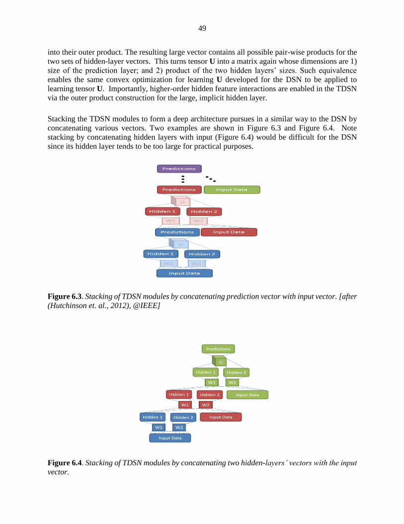
49

into their outer product. The resulting large vector contains all possible pair-wise products for the

two sets of hidden-layer vectors. This turns tensor U into a matrix again whose dimensions are 1)

size of the prediction layer; and 2) product of the two hidden layers’ sizes. Such equivalence

enables the same convex optimization for learning U developed for the DSN to be applied to

learning tensor U. Importantly, higher-order hidden feature interactions are enabled in the TDSN

via the outer product construction for the large, implicit hidden layer.

Stacking the TDSN modules to form a deep architecture pursues in a similar way to the DSN by

concatenating various vectors. Two examples are shown in Figure 6.3 and Figure 6.4. Note

stacking by concatenating hidden layers with input (Figure 6.4) would be difficult for the DSN

since its hidden layer tends to be too large for practical purposes.

Figure 6.3. Stacking of TDSN modules by concatenating prediction vector with input vector. [after

(Hutchinson et. al., 2012), @IEEE]

Figure 6.4. Stacking of TDSN modules by concatenating two hidden-layers’ vectors with the input

vector.

50

6.5 The Kernelized Deep Stacking Network

The DSN architecture has also recently been generalized to its kernelized version, which we call

the kernel-DSN (K-DSN) (Deng et al., 2012; Huang et al, 2013). The motivation of the extension

is to increase the size of the hidden units in each DSN module, yet without increasing the size of

the free parameters to learn. This goal can be easily accomplished using the kernel trick, resulting

in the K-DSN which we describe below.

In the DSN architecture reviewed above optimizing the weight matrix U given the hidden layers’

outputs in each module is a convex optimization problem. However, the problem of optimizing

weight matrix 𝑾 and thus the whole network is non-convex. In a recent extension of DSN, a tensor

structure was imposed, shifting most of the non-convex learning burden for 𝑾 to the convex

optimization of U (Hutchinson et al, 2012; 2013). In the new K-DSN extension, we completely

eliminate non-convex learning for 𝑾 using the kernel trick.

To derive the K-DSN architecture and the associated learning algorithm, we first take the bottom

module of DSN as an example and generalize the sigmoidal hidden layer 𝒉𝑖 = 𝜎(𝑾𝑇𝒙𝑖) in the

DSN module into a generic nonlinear mapping function 𝑮(𝑿) from the raw input feature 𝑿, with

high dimensionality in 𝑮(𝑿) (possibly infinite) determined only implicitly by a kernel function to

be chosen. Second, we formulate the constrained optimization problem of

minimize 1

2Tr[𝑬𝑬T] +

𝐶

2 𝑼T𝑼

subject to 𝐓-𝑼𝑇𝑮(𝑿) = E

Third, we make use of dual representations of the above constrained optimization problem to

obtain U = 𝐆T𝒂, where vector 𝒂 takes the following form

a = (𝐶𝑰 + 𝑲)−1𝑻

and 𝑲 = 𝑮(𝑿)𝑮T(𝑿) is a symmetric kernel matrix with elements Knm = gT(xn)𝑔(xm).

Finally, for each new input vector x in the test or dev set, we obtain the K-DSN (bottom) module’s

prediction as

y(x) = UT𝒈(𝒙) = 𝐚T𝑮(𝑿) 𝒈(𝒙)= 𝒌T(𝒙)(𝐶 𝑰 + 𝑲)−1𝑻

where the kernel vector 𝒌(𝒙) is so defined that its elements have values of 𝑘𝑛(𝒙) = 𝑘(𝒙𝑛, 𝒙) in

which 𝒙𝑛 is a training sample and 𝒙 is the current test sample.

For l-th module in K-DCN where 𝑙 ≥ 2, the kernel matrix is modified to

𝑲 = 𝑮 ([𝑿| 𝒀(𝑙−1)| 𝒀

(𝑙−2)|. . 𝒀(1)]) 𝑮T ([𝑿| 𝒀

(𝑙−1)| 𝒀(𝑙−2)|. . 𝒀

(1)]).

51

The key advantages of K-DSN can be analyzed as follows. First, unlike DSN which needs to

compute hidden units’ output, the K-DSN does not need to explicitly compute hidden units’ output

𝑮(𝑿) or 𝑮([𝑿| 𝒀(𝑙−1)| 𝒀

(𝑙−2)|. . 𝒀(1)]). When Gaussian kernels are used, kernel trick equivalently

gives us an infinite number of hidden units without the need to compute them explicitly. Further,

we no longer need to learn the lower-layer weight matrix 𝑾 in DSN as described in (Deng et al,

2012) and the kernel parameter (e.g., the single variance parameter 𝜎 in the Gaussian kernel)

makes K-DSN much less subject to overfitting than DSN. Figure 6.5 illustrates the basic

architecture of a K-DSN using the Gaussian kernel and using three modules.

Figure 6.5. An example architecture of the K-DSN with three modules each of which uses a

Gaussian kernel with different kernel parameters. [after (Deng. al., 2012), @IEEE]

The entire K-DSN with Gaussian kernels is characterized by two sets of module-dependent hyper-

parameters: 𝜎(𝑙) and 𝐶(𝑙) , the kernel smoothing parameter and regularization parameter,

respectively. While both parameters are intuitive and their tuning (via line search or leave-one-out

cross validation) is straightforward for a single bottom module, tuning the full network with all the

modules is more difficult. For example, if the bottom module is tuned too well, then adding more

modules would not benefit much. In contrast, when the lower modules are loosely tuned (i.e.,

relaxed from the results obtained from straightforward methods), the overall K-DSN often

performs much better. The experimental results reported by Deng et al. (2012) are obtained using

a set of empirically determined tuning schedules to adaptively regularize the K-DSN from bottom

to top modules.

The K-DSN described here has a set of highly desirable properties from the machine learning and

pattern recognition perspectives. It combines the power of deep learning and kernel learning in a

principled way and unlike the basic DSN there is no longer non-convex optimization problem

(1)

(2)

( ) = ( ( )) T( ( ))

( ) = ( ) T( );

(1)

(1)

(2)

(2) = ( (2)) T( (2))

(1) ( )

(1)

(2)

(2)

( )

( )

52

involved in training the K-DSN. The computation steps make the K-DSN easier to scale up for

parallel computing in distributed servers than the DSN and tensor-DSN. There are many fewer

parameters in the K-DSN to tune than in the DSN, T-DSN, and DNN, and there is no need for pre-

training. It is found in the study of (Deng et al., 2012) that regularization plays a much more

important role in the K-DSN than in the basic DSN and Tensor-DSN. Further, effective

regularization schedules developed for learning the K-DSN weights can be motivated by intuitive

insight from useful optimization tricks such as the heuristic in Rprop or resilient backpropagation

algorithm (Riedmiller and Braun, 1993).

However, as inherent in any kernel method, the scalability becomes an issue also for the K-DSN

as the training and testing samples become very large. A solution is provided in the study by Huang

et al. (2013), based on the use of random Fourier features, which possess the strong theoretical

property of approximating the Gaussian kernel while rendering efficient computation in both

training and evaluation of the K-DSN with large training samples. It is empirically demonstrated

that just like the conventional K-DSN exploiting rigorous Gaussian kernels, the use of random

Fourier features also enables successful stacking of kernel modules to form a deep architecture.

53

CHAPTER 7

SELECTED APPLICATIONS IN SPEECH

AND AUDIO PROCESSING

7.1 Acoustic Modeling for Speech Recognition As discussed in Chapter 2, speech recognition is the very first successful application of deep

learning methods at an industry scale. This success is a result of close academic-industrial

collaboration, initiated at Microsoft Research, with the involved researchers identifying and

acutely attending to the industrial need for large-scale deployment (Deng et al., 2009; Yu et al.,

2010c; Seide et al., 2011; Hinton et al, 2012; Dahl et al., 2012; Deng et al., 2013b). It is also a

result of carefully exploiting the strengths of the deep learning and the then-state-of-the-art speech

recognition technology, including notably the highly efficient decoding techniques.

Speech recognition has long been dominated by the GMM-HMM method, with an underlying

shallow or flat generative model of context-dependent GMMs and HMMs (e.g., Rabiner, 1989;

Juang et al., 1986; Deng et al., 1990, 1991). Neural networks once were a popular approach but

had not been competitive with the GMM-HMM (Waibel et al., 1989; Bourlard and Morgan, 1993;

Deng et al., 1994; Morgan, 2012). Generative models with deep hidden dynamics likewise have

also not been clearly competitive (e.g., Picone et al., 1999; Deng, 1998; Bridle et al. 1998; Deng

et al., 2006).

Deep learning and the DNN started making their impact in speech recognition in 2010, after close

collaborations between academic and industrial researchers; see reviews in (Hinton et al., 2012;

Deng et al., 2013c). The collaborative work started in phone recognition tasks (Mohamed et al.,

2009, 2010, 2012; Deng et al., 2010, 2013; Sivaram and Hermansky, 2012; Graves et al., 2013,

2013a; Sainath et al., 2011, 2013), demonstrating the power of hybrid DNN architectures discussed

in Chapter 5 and of subsequent new architectures with convolutional and recurrent structure. The

work also showed the importance of raw speech features of spectrogram --- back from the long-

popular MFCC features toward but not yet reaching the raw speech-waveform level (e.g.,

Sheikhzadeh and Deng, 1994; Jaitly and Hinton, 2011). The collaboration continued to large

vocabulary tasks with more convincing, highly positive results (Yu et al., 2010c; Dahl et al., 2011,

2012; Seide et al., 2011; Kubo et al., 2012; Hinton et al., 2012; Kingsbury et al., 2012; Deng et al.,

2013a, 2013b; Su et al., 2013; Yan et al., 2013; Liao et al., 2013). The success in large vocabulary

speech recognition is in large part attributed to the use of a very large DNN output layer structured

in the same way as the GMM-HMM speech units (senones), motivated initially by the speech

researchers’ desires to take advantage of the context-dependent phone modeling techniques that

have been proven to work well in the GMM-HMM framework, and to keep the change of the

already highly efficient decoder software’s infrastructure developed for the GMM-HMM systems

to a minimum. In the meantime, this body of work also demonstrated the possibility to reduce the

need for the DBN-like pre-training in effective learning of DNNs when a large amount of labeled

54

data is available. A combination of three factors helped to quickly spread the success of deep

learning in speech recognition to the entire speech industry and academia: 1) minimal decoder

changes required to deploy the new DNN-based speech recognizer due to the use of senones as the

DNN output; 2) significantly lowered errors compared with the then-state-of-the-art GMM-HMM

systems; and 3) reduced system complexity empowered by the DNN’s strong modeling power. By

the ICASSP-2013 timeframe, at least 15 major speech recognition groups worldwide confirmed

experimentally the success of DNNs with very large tasks and with the use of raw speech spectral

features other than MFCCs. The most notable groups include major industrial speech labs

worldwide: Microsoft (Seide et al, 2011; Chen et al., 2012; Deng et al., 2013b, 2013c; Yan et al.

2013; Yu et al., 2013b), IBM (Sainath et al., 2011, 2013, 2013b; Kingsbury et al., 2012; Saon et

al., 2013), Google (Jaitly et al., 2012; Dean et al., 2012; Heigold et al., 2013; Liao et al., 2013),

iFlyTek, and Baidu. Their results represent a new state-of-the-art in speech recognition widely

deployed in these companies’ voice products and services with extensive media coverage in recent

years.

In the remainder of this chapter, we review a wide range of speech recognition work based on deep

learning methods according to several major themes expressed in the section titles.

7.1.1 Back to primitive spectral features of speech

Deep learning, also referred as representation learning or (unsupervised) feature learning, sets an

important goal of automatic discovery of powerful features from raw input data independent of

application domains. For speech feature learning and for speech recognition, this goal is condensed

to the use of primitive spectral or possibly waveform features. Over the past 30 years or so, largely

“hand-crafted” transformations of speech spectrogram have led to significant accuracy

improvements in the GMM-based HMM systems, despite the known loss of information from the

raw speech data. The most successful transformation is the non-adaptive cosine transform, which

gave rise to Mel-frequency cepstral coefficients (MFCC) features. The cosine transform

approximately de-correlates feature components, which is important for the use of GMMs with

diagonal covariance matrices. However, when GMMs are replaced by deep learning models such

as DNNs, deep belief nets (DBNs), or deep autoencoders, such de-correlation becomes irrelevant

due to the very strength of the deep learning methods in modeling data correlation. As discussed

in detail in Chapter 4, early work of (Deng et al., 2010) demonstrated this strength and in particular

the benefit of spectrograms over MFCCs in effective coding of bottleneck speech features using

autoencoders in an unsupervised manner.

The pipeline from speech waveforms (raw speech features) to MFCCs and their temporal

differences goes through intermediate stages of log-spectra and then (Mel-warped) filter-banks,

with learned parameters based on the data. An important character of deep learning is to move

away from separate design of feature representations and of classifiers. This idea of jointly learning

classifier and feature transformation for speech recognition was already explored in early studies

on the GMM-HMM based systems; e.g., (Chengalvarayan and Deng, 1997; 1997a; Rathinavalu

and Deng, 1997). However, greater speech recognition performance gain is obtained only recently

in the recognizers empowered by deep learning methods. For example, Li et al., (2012) and Deng

et al., (2013a) showed significantly lowered speech recognition errors using large-scale DNNs

55

when moving from the MFCC features back to more primitive (Mel-scaled) filter-bank features.

These results indicate that DNNs can learn a better transformation than the original fixed cosine

transform from the Mel-scaled filter-bank features.

Compared with MFCCs, “raw” spectral features not only retain more information, but also enable

the use of convolution and pooling operations to represent and handle some typical speech

invariance and variability --- e.g., vocal tract length differences across speakers, distinct speaking

styles causing formant undershoot or overshoot, etc. --- expressed explicitly in the frequency

domain. For example, the convolutional neural network (CNN) can only be meaningfully and

effectively applied to speech recognition (Abdel-Hamid et al., 2012; 2013, 2013a; Deng et al.,

2013) when spectral features, instead of MFCC features, are used.

More recently, Sainath et al. (2013b) went one step further toward raw features by learning the

parameters that define the filter-banks on power spectra. That is, rather than using Mel-warped

filter-bank features as the input features as in (Abdel-Hamid et al., 2012; 2013; Li et al., 2012;

Chengalvarayan and Deng, 1997), the weights corresponding to the Mel-scale filters are only used

to initialize the parameters, which are subsequently learned together with the rest of the deep

network as the classifier. The overall architecture of the jointly learned feature generator and

classifier is shown in Figure 7.1. Substantial speech recognition error reduction is reported in

(Sainath et al., 2013b).

Figure 7.1. Illustration of the joint learning of filter parameters and the rest of the deep network.

Adopted from [after (Sainath et al., 2013b), @IEEE].

56

It has been shown that not only learning the spectral aspect of the features are beneficial for speech

recognition, learning the temporal aspect of the features is also helpful (Siniscalchi et al. 2013).

Further, Yu et al. (2013a) carefully analyzed the properties of different layers in the DNN as the

layer-wise extracted features starting from the lower raw filter-bank features. They found that the

improved speech recognition accuracy achieved by the DNNs partially attributes to DNN’s ability

to extract discriminative internal representations that are robust to the many sources of variability

in speech signals. They also show that these representations become increasingly insensitive to

small perturbations in the input at higher layers, which helps to achieve better speech recognition

accuracy.

To the extreme end, deep learning would promote to use the lowest level of raw features of speech,

i.e., speech sound waveforms, for speech recognition, and learn the transformation automatically.

As an initial attempt toward this goal the study carried out by Jaitly and Hinton (2011) makes use

of speech sound waves as the raw input feature to an RBM with a convolutional structure as the

classifier. With the use of rectified linear units in the hidden layer (Glorot et al., 2011), it is possible,

to a limited extent, to automatically normalize the amplitude variation in the waveform signal.

Although the final results are disappointing, the work shows that much work is needed along this

direction. For example, just as demonstrated by Sainath et al. (2013b) that the use of raw spectra

as features requires additional attention in normalization than MFCCs, the use of speech

waveforms demands even more attention (e.g., Sheikhzadeh and Deng, 1994). This is true for both

GMM-based and deep learning based methods.

7.1.2 The DNN-HMM architecture vs. use of DNN-derived

features

Another major theme in the recent studies reported in the literature on applying deep learning

methods to speech recognition is two disparate ways of using the DNN: 1) Direct applications of

the DNN-HMM architecture as discussed in Chapter 5.3 to perform speech recognition; and 2)

The use of DNNs to extract or derive features, which are then fed into a separate sequence classifier.

In the speech recognition literature (e.g., Bourlard and Morgan, 1993), a system, in which a neural

network’s output is directly used to estimate the emission probabilities of an HMM, is often called

an ANN/HMM hybrid system. This should be distinguished from the use of “hybrid” in Chapter

5 and throughout this book, where a hybrid of unsupervised pre-training and of supervised fine

tuning is exploited to learn the parameters of DNNs.

The DNN-HMM architecture as a recognizer

An early DNN-HMM architecture (Mohamed et al., 2009) was presented at the NIPS Workshop

(Deng, Yu, Hinton, 2009), developed, analyzed, and assisted by University of Toronto and MSR

speech researchers. In this work, a five-layer DNN (called the DBN in the paper) was used to

replace the Gaussian mixture models in the GMM-HMM system, and the monophone state was

used as the modeling unit. Although monophones are generally accepted as a weaker phonetic

representation than triphones, the DNN-HMM approach with monophones was shown to achieve

higher phone recognition accuracy than the state-of-the-art triphone GMM-HMM systems. Further,

57

the DNN results were found to be slightly superior to the then-best-performing single system based

on the generative hidden trajectory model (HTM) in the literature (Deng et al., 2006, 2007)

evaluated on the same, commonly used TIMIT task by many speech researchers (e.g., Ostendorf

et al., 1996; Deng et al., 2006; Sainath et al., 2011a). At MSR, Redmond, the error patterns

produced by these two separate systems (the DNN vs. the HTM) were carefully analyzed and

found to be very different, reflecting distinct core capabilities of the two approaches and igniting

intensive further studies on the DNN-HMM approach described below.

MSR and University of Toronto researchers (Yu et al., 2010c; Dahl et al., 2011, 2012) extended

the DNN-HMM system from the monophone phonetic representation of the DNN outputs to the

triphone or context-dependent counterpart and from phone recognition to large vocabulary speech

recognition. Experiments conducted at MSR on the 24-hr and 48-hr Bing mobile voice search

datasets collected under the real usage scenario demonstrate that the context-dependent DNN-

HMM significantly outperforms the state-of-the-art HMM system. Three factors, in addition to the

use of the DNN, contribute to the success: the use of triphones as the DNN modeling units, the use

of the best available tri-phone GMM-HMM to generate the tri-phone state alignment, and the

effective exploitation of a long window of input features. Experiments also indicate that the

decoding time of a five-layer DNN-HMM is almost the same as that of the state-of-the-art triphone

GMM-HMM.

The success was quickly extended to large vocabulary speech recognition tasks with hundreds and

even thousands of hours of training set and with thousands of tri-phone states, including the

Switchboard and Broadcast News databases, and Google’s voice search and YouTube tasks (Seide

et al., 2011; Sainath et al., 2011; Jaitly et al., 2012; Hinton et al., 2012; Deng et al., 2013a; Sainath

et al, 2013). For example, on the Switchboard benchmark, the context-dependent DNN-HMM

(CD-DNN-HMM) is shown to cut error by one third compared to the state-of-the-art GMM-HMM

system (Seide et al., 2011). As a summary, we show in Table 7.1 some quantitative recognition

error rates produced by the DNN-HMM architecture in comparison with those by the previous

state of the art systems based on the generative models. Note from sub-tables A to D, the training

data are increased approximately one order of magnitude from one task to the next. Not only the

computation scales up well (i.e., almost linearly) with the training size, but most importantly the

relative error rate reduction increases substantially with increasing amounts of training data ---

from approximately 10% to 20%, and then to 30%. This set of results highlight the strongly

desirable properties of the DNN-based methods, despite the conceptual simplicity of the overall

DNN-HMM architecture and some known weaknesses.

58

Table 7.1. Comparisons of the DNN-HMM architecture with the generative model (e.g., the GMM-

HMM) in terms of phone or word recognition error rates. From sub-tables A to D, the training

data are increased approximately three orders of magnitudes.

The use of DNN-derived features in a separate recognizer

One clear weakness of the above DNN-HMM architecture for speech recognition is that much of

the highly effective techniques for the GMM-HMM systems, including discriminative training (in

both feature space and model space), unsupervised speaker adaptation, noise robustness, and

scalable batch training tools for big training data, developed over the past 20 some years may not

be directly applicable to the new systems although similar techniques have been recently

developed for DNN-HMMs. To remedy this problem, the “tandem” approach, developed

originally by Hermansky et al. (2000), has been adopted, where the output of the neural networks

in the form of posterior probabilities of the phone classes, are used, often in conjunction with the

acoustic features to form new augmented input features, in a separate GMM-HMM system.

This tandem approach is used by Vinyals and Ravuri (2011) where a DNN’s outputs are extracted

to serve as the features for mismatched noisy speech. It is reported that DNNs outperform the

neural networks with a single hidden layer under the clean condition, but the gains slowly diminish

as the noise level is increased. Furthermore, using MFCCs in conjunction with the posteriors

computed from DNNs outperforms using the DNN features alone in low to moderate noise

conditions with the tandem architecture. Comparisons of such tandem approach with the direct

DNN-HMM approach are made by Tüske et al. (2012) and Imseng et al. (2013).

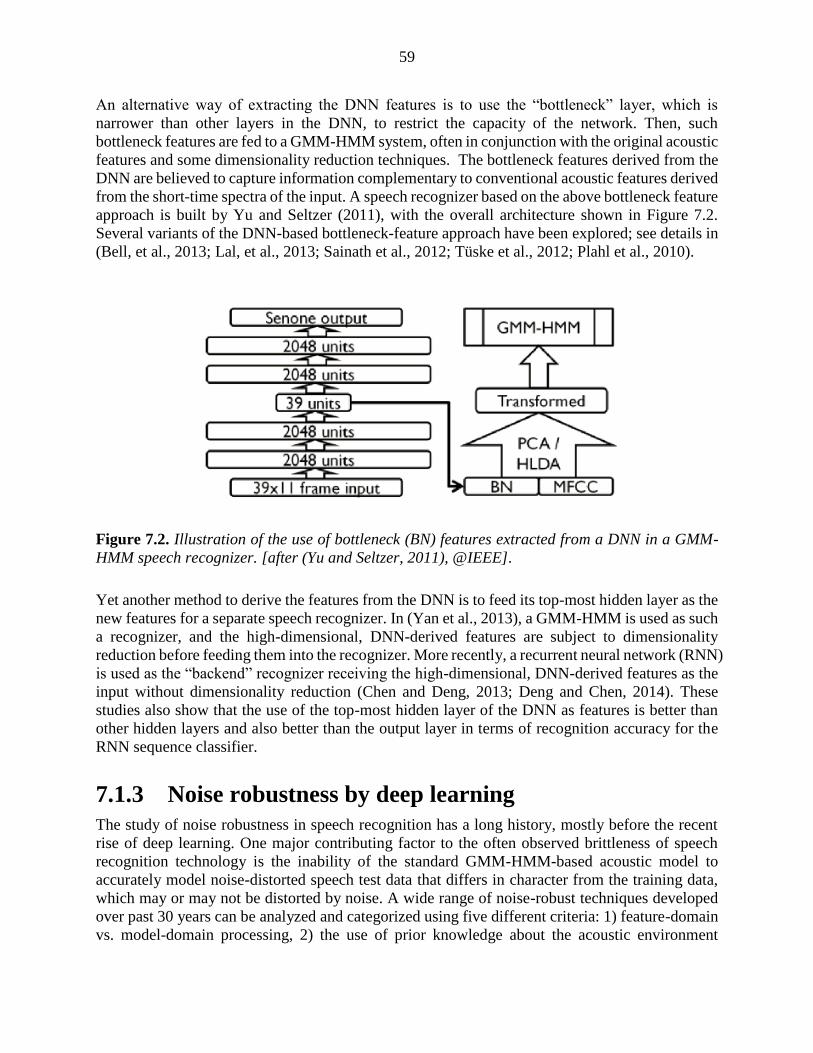
59

An alternative way of extracting the DNN features is to use the “bottleneck” layer, which is

narrower than other layers in the DNN, to restrict the capacity of the network. Then, such

bottleneck features are fed to a GMM-HMM system, often in conjunction with the original acoustic

features and some dimensionality reduction techniques. The bottleneck features derived from the

DNN are believed to capture information complementary to conventional acoustic features derived

from the short-time spectra of the input. A speech recognizer based on the above bottleneck feature

approach is built by Yu and Seltzer (2011), with the overall architecture shown in Figure 7.2.

Several variants of the DNN-based bottleneck-feature approach have been explored; see details in

(Bell, et al., 2013; Lal, et al., 2013; Sainath et al., 2012; Tüske et al., 2012; Plahl et al., 2010).

Figure 7.2. Illustration of the use of bottleneck (BN) features extracted from a DNN in a GMM-

HMM speech recognizer. [after (Yu and Seltzer, 2011), @IEEE].

Yet another method to derive the features from the DNN is to feed its top-most hidden layer as the

new features for a separate speech recognizer. In (Yan et al., 2013), a GMM-HMM is used as such

a recognizer, and the high-dimensional, DNN-derived features are subject to dimensionality

reduction before feeding them into the recognizer. More recently, a recurrent neural network (RNN)

is used as the “backend” recognizer receiving the high-dimensional, DNN-derived features as the

input without dimensionality reduction (Chen and Deng, 2013; Deng and Chen, 2014). These

studies also show that the use of the top-most hidden layer of the DNN as features is better than

other hidden layers and also better than the output layer in terms of recognition accuracy for the

RNN sequence classifier.

7.1.3 Noise robustness by deep learning

The study of noise robustness in speech recognition has a long history, mostly before the recent

rise of deep learning. One major contributing factor to the often observed brittleness of speech

recognition technology is the inability of the standard GMM-HMM-based acoustic model to

accurately model noise-distorted speech test data that differs in character from the training data,

which may or may not be distorted by noise. A wide range of noise-robust techniques developed

over past 30 years can be analyzed and categorized using five different criteria: 1) feature-domain

vs. model-domain processing, 2) the use of prior knowledge about the acoustic environment

60

distortion, 3) the use of explicit environment-distortion models, 4) deterministic vs. uncertainty

processing, and 5) the use of acoustic models trained jointly with the same feature enhancement

or model adaptation process used in the testing stage. See a comprehensive review in (Li et al.,

2014) and some additional review literature or original work in (Gales, 2011; Lu et al., 2013;

Yoshioka and Nakatani, 2013; Wang and Gales, 2012; Zhao and Juang, 2012; Hain et al., 2012;

van Dalen, et al., 2011; Yu et al., 2009; Acero et al., 2000; Deng et al., 2000).

Many of the model-domain techniques developed for GMM-HMMs (e.g., model-domain noise

robustness techniques surveyed by Li et al. (2014) and Gales (2011)), are not directly applicable

to the new deep learning models for speech recognition. The feature-domain techniques, however,

can be directly applied to the DNN system. A detailed investigation of the use of DNNs for noise

robust speech recognition in the feature domain is reported by Seltzer et al. (2013), who apply the

C-MMSE (Yu et al., 2008) feature enhancement algorithm on the input feature used in the DNN.

By processing both the training and testing data with the same algorithm, any consistent errors or

artifacts introduced by the enhancement algorithm can be learned by the DNN-HMM recognizer.

This study also successfully explores the use of the noise aware training paradigm for training the

DNN, where each observation is augmented with an estimate of the noise. Strong results are

obtained on the Aurora4 task. More recently, Kashiwagi et al. (2013) applies the SPLICE feature

enhancement technique (Deng et al., 2000, 2001) to a DNN speech recognizer. In that study the

DNN’s output layer is determined on the clean data instead of the noisy data as in the study by

Seltzer et al. (2013).

Besides DNN, other deep architectures have also been proposed to perform feature enhancement

and noise-robust speech recognition. For example, Mass et al. (2012) applied a deep recurrent auto

encoder neural network to remove noise in the input features for robust speech recognition. The

model is trained on stereo (noisy and clean) speech features to predict clean features given noisy

input, similar to the SPLICE setup but using a deep model instead of a GMM. Vinyals and Ravuri

(2011) investigated the tandem approaches to noise-robust speech recognition, where DNNs are

trained directly with noisy speech to generate posterior features.

7.1.4 Output representations in the DNN

Most deep learning methods for speech recognition and other information processing applications

have focused on learning representations from input acoustic features without paying attention to

output representations. The recent 2013 NIPS Workshop on Learning Output Representations

(http://nips.cc/Conferences/2013/Program/event.php?ID=3714) was dedicated to bridging this gap.

For example, the Deep Visual-Semantic Embedding Model described in (Frome et al., 2013, to be

discussed more in Chapter 11) exploits continuous-valued output representations obtained from

the text embeddings to assist in the branch of the deep network for classifying images. For speech

recognition, importance of designing effective linguistic representations for the output layers of

deep networks is highlighted in (Deng, 2013).

Most current DNN systems use a high-dimensional output representation to match the

context-dependent phonetic states in the HMMs. For this reason, the output layer evaluation

can cost 1/3 of the total computation time. To improve the decoding speed, techniques such

as low-rank approximation is typically applied to the output layer. In (Sainath et al., 2013c)

61

and (Xue et al., 2013), the DNN with high-dimensional output layer was trained first. The singular

value decomposition (SVD)-based dimension reduction technique was then performed on the large

output-layer matrix. The resulting matrices are further combined and as the result the original

large weight matrix is approximated by a product of two much smaller matrices. This technique

in essence converts the original large output layer to two layers – a bottleneck linear layer and a

nonlinear output layer --- both with smaller weight matrices. The converted DNN with reduced

dimensionality in is further refined. The experimental results show that no speech recognition

accuracy reduction was observed even when the size is cut to 1/3, while the run-time

computation is significantly reduced.

The output representations for speech recognition can benefit from the structured design of the

symbolic or phonological units of speech as presented in (Deng, 2013). The rich phonological

structure of symbolic nature in human speech has been well known for many years. Likewise, it

has also been well understood for a long time that the use of phonetic or its finer state sequences,

even with contextual dependency, in engineering speech recognition systems, is inadequate in

representing such rich structure (e.g., Deng and Erler, 1992; Ostendorf, 1999; Sun and Deng, 2002),

and thus leaving a promising open direction to improve the speech recognition systems’

performance. Basic theories about the internal structure of speech sounds and their relevance to

speech recognition technology in terms of the specification, design, and learning of possible output

representations of the underlying speech model for speech target sequences are surveyed in (Deng

and O’Shaughnessy, 2003) and more recently in (Deng, 2013).

There has been a growing body of deep learning work in speech recognition with their focus placed

on designing output representations related to linguistic structure. In (Wang and Sim, 2013; 2014),

a limitation of the output representation design, based on the context-dependent phone units as

proposed by Dahl et al. (2012), is recognized and a solution is offered. The root cause of this

limitation is that all context-dependent phone states within a cluster created by the decision tree

share the same set of parameters and this reduces its resolution power for fine-grained states during

the decoding phase. The solution proposed formulates output representations of the context-

dependent DNN as an instance of the canonical state modeling technique, making use of broad

phonetic classes. First, triphones are clustered into multiple sets of shorter bi-phones using broad

phone contexts. Then, the DNN is trained to discriminate the bi-phones within each set. Logistic

regression is used to transform the canonical states into the detailed triphone state output

probabilities. That is, the overall design of the output representation of the context-dependent DNN

is hierarchical in nature, solving both the data sparseness and low-resolution problems at the same

time.

Related work on designing the output linguistic representations for speech recognition can be

found in (Ko and Mak, 2013) and in (McGraw et al., 2013). While the designs are in the context

of GMM-HMM-based speech recognition systems, they both can be extended to deep learning

models.

62

7.1.5 Adaptation of the DNN-based speech recognizers

The DNN-HMM is an advanced version of the artificial neural network and HMM hybrid system

developed in 1990s, for which several adaptation techniques have been developed. Most of these

techniques are based on linear transformation of the network weights of either input or output

layers. Some initial work on DNN adaptation makes use of the same or related linear

transformation methods (e.g., Yao et al., 2012; 2013a). However, compared with the earlier

narrower and shallower neural network systems, the DNN-HMM has significantly more

parameters due to wider and deeper hidden layers used and the much larger output layer designed

to model context dependent phones and states. This difference casts additional challenges to

adapting the DNN-HMM, especially when the adaptation data is small. Here we discuss three

recent studies on overcoming such challenges in adapting the large-sized DNN weights in three

distinct ways.

Yu et al. (2013b) proposed a regularized adaptation technique for DNNs. It adapts the DNN

weights conservatively by forcing the distribution estimated from the adapted model to be close to

that estimated from those before the adaptation. This constraint is realized by adding Kullback–

Leibler divergence (KLD) regularization to the adaptation criterion. This type of regularization is

shown to be equivalent to a modification of the target distribution in the conventional

backpropagation algorithm and thus the training of the DNN remains largely unchanged. The new

target distribution is derived to be a linear interpolation of the distribution estimated from the

model before adaptation and the ground truth alignment of the adaptation data. This interpolation

prevents overtraining by keeping the adapted model from straying too far from the speaker-

independent model. This type of adaptation differs from L2 regularization which constrains the

model parameters themselves rather than the output probabilities.

In (Siniscalchi et al., 2013a), adaptation of the DNN is applied not on the conventional network

weights by on the hidden activation functions. In this way, the main limitation of current adaptation

techniques based on adaptable linear transformation of the network weights in either the input or

the output layer is effectively overcome, since the new method only needs to adapt limited hidden

activation function.

Most recently, Saon et al. (2013) explore a new and highly effective method in adapting DNNs for

speech recognition. The method combines I-vector features with fMLLR (feature-domain Max-

Likelihood Linear Regression) features as the input into a DNN. I-vectors or (speaker) identity

vectors are commonly used for speaker verification and speaker recognition applications, as they

encapsulate relevant information about a speaker’s identity in a low-dimensional feature vector.

The fMLLR is an effective adaptation technique developed for GMM-HMM systems. Since I-

vectors do not obey locality in frequency, they must be combined carefully with the fMLLR

features that obey locality. The architecture of multi-scale CNN-DNN is shown to be effective for

the combination of these two different types of features. During both training and decoding, the

speaker-specific I-vector is appended to the frame-based fMLLR features.

63

7.1.6 Better architectures and nonlinear units

Over recent years, since the success of the (fully-connected) DNN-HMM hybrid system was

demonstrated in (Mohamed et al., 2009, 2012; Deng et al., 2009; Yu et al., 2010; Dahl et al., 2011,

2012; Seide et al., 2011; Sainath et al., 2011, 2012; Hinton et al., 2012), many new architectures

and nonlinear units have been proposed and evaluated for speech recognition. Here we provide an

overview of this progress, extending the overview provided in (Deng et al., 2013b).

The tensor version of the DNN is reported by Yu et al. (2012c, 2013), which extends the

conventional DNN by replacing one or more of its layers with a double-projection layer and a

tensor layer. In the double-projection layer, each input vector is projected into two nonlinear

subspaces. In the tensor layer, two subspace projections interact with each other and jointly predict

the next layer in the overall deep architecture. An approach is developed to map the tensor layers

to the conventional sigmoid layers so that the former can be treated and trained in a similar way to

the latter. With this mapping the tensor version of the DNN can be treated as the DNN augmented

with double-projection layers so that the backpropagation learning algorithm can be cleanly

derived and relatively easily implemented.

A related architecture to the above is the tensor version of the DSN described in Chapter 6, also

usefully applied to speech classification and recognition (Hutchinson et al., 2012, 2013). The same

approach applies to mapping the tensor layers (i.e., the upper layer in each of the many modules

in the DSN context) to the conventional sigmoid layers. Again, this mapping simplifies the training

algorithm so that it becomes not so far apart from that for the DSN.

As discussed in Chapter 3.2, the concept of convolution in time was originated in the TDNN (time-

delay neural network) as a shallow neural network (Lang et al., 1990; Waibel et al., 1989)

developed during early days of speech recognition. Only recently and when deep architectures (e.g.

deep Convolutional Neural Network or deep CNN) were used, it has been found that frequency-

dimension weight sharing is more effective for high-performance phone recognition, when the

HMM is used to handle the time variability, than time-domain weight sharing as in the previous

TDNN in which the HMM was not used (Abdel-Hamid et al., 2012, 2013, 2013a; Deng et al.,

2013). These studies also show that designing the pooling in the deep CNN to properly trade-off

between invariance to vocal tract length and discrimination between speech sounds, together with

a regularization technique of “dropout” (Hinton et al., 2012a), leads to even better phone

recognition performance. This set of work further points to the direction of trading-off between

trajectory discrimination and invariance expressed in the whole dynamic pattern of speech defined

in mixed time and frequency domains using convolution and pooling. Moreover, the most recent

studies reported in (Sainath et al., 2013, 2013a; 2013e) show that CNNs also benefit large

vocabulary continuous speech recognition. They further demonstrate that multiple convolutional

layers provide even more improvement when the convolutional layers use a large number of

convolution kernels or feature maps. In particular, Sainath et al. (2013e) extensively explored

many variants of the deep CNN. In combination with several novel methods the deep CNN is

shown to produce state of the art results in a few large vocabulary speech recognition tasks.

In addition to the DNN, CNN, and DSN, as well as their tensor versions, other deep models have

also been developed and reported in the literature for speech recognition. For example, the deep-

64

structured CRF, which stacks many layers of CRFs, have been usefully applied to the task of

language identification (Yu et al., 2010), phone recognition (Yu and Deng, 2010), sequential

labeling in natural language processing (Yu et al., 2010a), and confidence calibration in speech

recognition (Yu et al., 2010b). More recently, Demuynck and Triefenbach (2013) developed the

deep GMM architecture, where the aspects of DNNs that lead to strong performance are extracted

and applied to build hierarchical GMMs. They show that by going “deep and wide” and feeding

windowed probabilities of a lower layer of GMMs to a higher layer of GMMs, the performance of

the deep-GMM system can be made comparable to a DNN. One advantage of staying in the GMM

space is that the decades of work in GMM adaptation and discriminative learning remains

applicable.

Perhaps the most notable deep architecture among all is the recurrent neural network (RNN) as

well as its stacked or deep version (Graves et al., 2013, 2013a; Hermans and Schrauwen, 2013).

While the RNN saw its early success in phone recognition (Robinson, 1994), it was not easy to

duplicate due to the intricacy in training, let alone to scale up for larger speech recognition tasks.

Learning algorithms for the RNN have been dramatically improved since then, and much better

results have been obtained recently using the RNN (Graves, et al, 2006; Maas et al., 2012; Chen

and Deng, 2013), especially when the bi-directional LSTM (long short-term memory) is used

(Graves et al., 2013, 2013a). The basic information flow in the bi-directional RNN and a cell of

LSTM is shown in Figures 7.3 and 7.4 respectively.

Figure 7.3. Information flow in the bi-directional RNN, with both diagrammatic and mathematical

descriptions. W’s are weight matrices, not shown but can be easily inferred in the diagram. [after

(Graves et al., 2013), @IEEE].

65

Figure 7.4. Information flow in an LSTM unit of the RNN, with both diagrammatic and

mathematical descriptions. W’s are weight matrices, not shown but can easily be inferred in the

diagram. [after (Graves et al., 2013), @IEEE].

Learning the RNN parameters is known to be difficult due to vanishing or exploding gradients

(Pascanu et al., 2013). Chen and Deng (2013) and Deng and Chen (2014) developed a primal-dual

training method that formulates the learning of the RNN as a formal optimization problem, where

cross entropy is maximized subject to the condition that the infinity norm of the recurrent matrix

of the RNN is less than a fixed value to guarantee the stability of RNN dynamics. Experimental

results on phone recognition demonstrate: 1) the primal-dual technique is highly effective in

learning RNNs, with superior performance to the earlier heuristic method of truncating the size of

the gradient; 2) The use of a DNN to compute high-level features of speech data to feed into the

RNN gives much higher accuracy than without using the DNN; and 3) The accuracy drops

progressively as the DNN features are extracted from higher to lower hidden layers of the DNN.

A special case of the RNN is reservoir models or echo state networks, where the output layers are

fixed to be linear instead of nonlinear as in the regular RNN, and where the recurrent matrices are

carefully designed but not learned. The input matrices are also fixed and not learned, due partly to

the difficulty of learning. Only the weight matrices between the hidden and output layers are

learned. Since the output layer is linear, the learning is very efficient and with global optimum

66

achievable by a closed-form solution. But due to the fact that many parameters are not learned, the

hidden layer needs to be very large in order to obtain good results. Triefenbach et al. (2013) applied

such models to phone recognition, with reasonably good accuracy obtained.

Palangi et al. (2013a) presented an improved version of the reservoir model by learning both the

input and recurrent matrices which were fixed in the previous model that makes use of the linear

output (or readout) units to simplify the learning of only the output matrix in the RNN. Rather, a

special technique is devised that takes advantage of the linearity in the output units in the reservoir

model to learn the input and recurrent matrices. Compared with the backpropagation through time

(BPTT) algorithm commonly used in learning the general RNNs, the proposed technique makes

use of the linearity in the output units to provide constraints among various matrices in the RNN,

enabling the computation of the gradients as the learning signal in an analytical form instead of by

recursion as in the BPTT.

In addition to the recent innovations in better architectures of deep learning models for speech

recognition reviewed above, there is also a growing body of work on developing and implementing

better nonlinear units. Although sigmoidal and tanh functions are the most commonly used

nonlinear types in DNNs their limitations are well known. For example, it is slow to learn the

whole network due to weak gradients when the units are close to saturation in both directions.

Jaitly and Hinton (2011) appear to be the first to apply the rectified linear units (ReLU) in the

DNNs to speech recognition to overcome the weakness of the sigmoidal units. ReLU refers to the

units in a neural network that use the activation function of𝑓(𝑥) = max(0, 𝑥). Dahl et al. (2013)

and Mass et al. (2013) successfully applied ReLU to large vocabulary speech recognition, with the

best accuracy obtained when combining ReLU with the “Dropout” regularization technique.

Another new type of DNN units demonstrated more recently to be useful for speech recognition is

the “maxout” units, which were used for forming the deep maxout network as described in (Miao

et al., 2013). A deep maxout network consists of multiple layers which generate hidden activations

via the maximum or “maxout” operation over a fixed number of weighted inputs called a “group”.

This is the same operation as the max pooling used in the CNN as discussed earlier for both speech

recognition and computer vision. The maximal value within each group is taken as the output from

the previous layer. Most recently, Zheng et al. (2014) generalize the above “maxout” units to two

new types. The “soft-maxout” type of units replace the original max operation with the soft-max

function. The second, p-norm type of units used the nonlinearity of y = ||x||p . It is shown

experimentally that the p-norm units with p=2 perform consistently better than the maxout, tanh,

and ReLU units.

Finally, Srivastava et al. (2013) propose yet another new type of nonlinear units, called winner-

take-all units. Here, local competition among neighboring neurons are incorporated into the

otherwise regular feed-forward architecture, which is then trained via backpropagation with

different gradients than the normal one. Winner-take-all is an interesting new form of nonlinearity,

and it forms groups of (typically two) neurons where all the neurons in a group are made zero-

valued except the one with the largest value. Experiments show that the network does not forget

as much as networks with standard sigmoidal nonlinearity. This new type of nonlinear units are

yet to be evaluated in speech recognition tasks.

67

7.1.7 Better optimization and regularization

Another area where significant advances are made recently in applying deep learning to acoustic

model for speech recognition is on optimization criteria and methods, as well as on the related

regularization techniques to help prevent overfitting during the deep network training.

One of the early studies on DNNs for speech recognition, conducted at Microsoft Research and

reported in (Mohamed et al., 2010), first recognizes the mismatch between the desired error rate

and the cross-entropy training criterion in the conventional DNN training. The solution is provided

by replacing the frame-based, cross-entropy training criterion with the full-sequence-based

maximum mutual information optimization objective. Equivalently, this amounts to putting the

model of conditional random field (CRF) at the top of the DNN, replacing the original softmax

layer which naturally leads to cross entropy. (Note the DNN was called the DBN in the paper).

This new sequential discriminative learning technique is developed to jointly optimize the DNN

weights, CRF transition weights, and bi-phone language model. Importantly, the speech task is

defined in TIMIT, with the use of a simple bi-phone-gram “language” model. The simplicity of

the bi-gram language model enables the full-sequence training to carry out without the need to use

lattices, drastically reducing the training complexity.

As another way to motivate the full-sequence training method of (Mohamed et al., 2010), we note

that the earlier DNN phone recognition experiments made use of the standard frame-based

objective function in static pattern classification, cross-entropy, to optimize the DNN weights. The

transition parameters and language model scores were obtained from an HMM and were trained

independently of the DNN weights. However, it has been known during the long history of the

HMM research that sequence classification criteria can be very helpful in improving speech and

phone recognition accuracy. This is because the sequence classification criteria are more directly

correlated with the performance measure (e.g., the overall word or phone error rate) than frame-

level criteria. More specifically, the use of frame-level cross entropy to train the DNN for phone

sequence recognition does not explicitly take into account the fact that the neighboring frames

have smaller distances between the assigned probability distributions over phone class labels. To

overcome this deficiency, one can optimize the conditional probability of the whole sequence of

labels, given the whole visible feature utterance or equivalent the hidden feature

sequence extracted by DNN. To optimize the log conditional probability on the training data, the

gradient can be taken over the activation parameters, transition parameters and lower-layer weights,

and then pursue back-propagation of the error defined at the sentence level. We remark that in a

much earlier study (LeCun et al., 1998), combining a neural network with a CRF-like structure

was done, where the mathematical formulation appears to include CRFs as a special case. Also,

the benefit of using the full-sequence classification criteria was shown earlier on shallow neural

networks in (Kingsbury 2009; Prabhavalkar and Fosler-Lussier, 2010).

In implementing the above full-sequence learning algorithm for the DNN system as described in

(Mohamed et al., 2010), the DNN weights are initialized using the frame-level cross entropy as

the objective. The transition parameters are initialized from the combination of the HMM

transition matrices and the “bi-phone language” model scores, and are then further optimized by

tuning the transition features while fixing the DNN weights before the joint optimization. Using

68

joint optimization with careful scheduling to reduce overfitting, it is shown that the full-sequence

training outperforms the DNN trained with frame-level cross entropy by approximately 5%

relative (Mohamed et al., 2010). Without the effort to reduce overfitting, it is found that the DNN

trained with MMI is much more prone to overfitting than that trained with frame-level cross

entropy. This is because the correlations across frames in speech tend to be different among the

training, development, and test data. Importantly, such differences do not show when frame-based

objective functions are used for training.

For large vocabulary speech recognition where more complex language models are in use, the

optimization methods for full-sequence training of the DNN-HMM are much more sophisticated.

Kingsbury et al. (2012) reported the first success of such training using parallel, second-order,

Hessian-free optimization techniques, which are carefully implemented for large vocabulary

speech recognition. Sainath et al. (2013d) improved and speeded up the Hessian-free techniques

by reducing the number of Krylov subspace solver iterations (Vinyals and Povey, 2012), which

are used for implicit estimation of the Hessian. They also use sampling methods to decrease the

amount of training data to speed up the training. While the batch-mode, second-order Hessian-free

techniques prove successful for full-sequence training of large-scale DNN-HMM systems, the

success of the first-order stochastic gradient descent methods is also reported recently (Su et al.,

2013). It is found that heuristics are needed to handle the problem of lattice sparseness. That is,

the DNN must be adjusted to the updated numerator lattices by additional iterations of frame-based

cross-entropy training. Further, artificial silence arcs need to be added to the denominator lattices,

or the maximum mutual information objective function needs to be smoothed with the frame-based

cross entropy objective. The conclusion is that for large vocabulary speech recognition tasks with

sparse lattices, the implementation of the sequence training requires much greater engineering

skills than the small tasks such as reported in (Mohamed et al., 2010), although the objective

function as well as the gradient derivation are essentially the same. Similar conclusions are reached

by Vesely et al. (2013) when carrying out full-sequence training of DNN-HMMs for large-

vocabulary speech recognition. However, different heuristics from (Su et al., 2013) are shown to

be effective in the training. Separately, Wiesler et al. (2013) investigated the Hessian-free

optimization method for training the DNN with the cross-entropy objective and empirically

analyzed the properties of the method. And finally, Dognin and Goel (2013) combined stochastic

average gradient and Hessian-free optimization for sequence training of deep neural networks with

success in that the training procedure converges in about half the time compared with the full

Hessian-free sequence training.

For large DNN-HMM systems with either frame-level or sequence-level optimization objectives,

speeding up the training is essential to take advantage of large amounts of training data and of

large model sizes. In addition to the methods described above, Dean et al. (2012) reported the use

of the asynchronous stochastic gradient descent (ASGD) method, the adaptive gradient descent

(Adagrad) method, and the large-scale limited-memory BFGS (L-BFGS) method for very large

vocabulary speech recognition. Sainath et al. (2013) provided a review of a wide range of

optimization methods for speeding up the training of DNN-based systems for large speech

recognition tasks.

In addition to the advances described above focusing on optimization with the fully supervised

learning paradigm, where all training data contain the label information, the semi-supervised

69

training paradigm is also exploited for learning DNN-HMM systems for speech recognition. Liao

et al. (2013) reported the exploration of using semi-supervised training on the DNN-HMM system

for the very challenging task of recognizing YouTube speech. The main technique is based on the

use of “island of confidence” filtering heuristics to select useful training segments. Separately,

semi-supervised training of DNNs is explored by Vesely et al. (2013), where self-training

strategies are used as the basis for data selection using both the utterance-level and frame-level

confidences. Frame-selection based on per-frame confidences derived from confusion in a lattice

is found beneficial. Huang et al. (2013) reported another variant of semi-supervised training

technique in which multi-system combination and confidence recalibration is applied to select the

training data. Further, Thomas et al. (2013) overcome the problem of lacking sufficient training

data for acoustic modeling in a number of low-resource scenarios. They make use of transcribed

multilingual data and semi-supervised training to build the proposed feature front-ends for

subsequent speech recognition.

Finally, we see important progress in deep learning based speech recognition in recent years with

the introduction of new regularization methods based on “dropout” originally proposed by Hinton

et al., (2012a). Overfitting is very common in DNN training and co-adaptation is prevalent within

the DNN with multiple activations adapting together to explain input acoustic data. Dropout is a

technique to limit co-adaptation. It operates as follows. On each training instance, each hidden unit

is randomly omitted with a fixed probability (e.g., p=0.5). Then, decoding is done normally except

with straightforward scaling of the DNN weights (by a factor of 1-p). Alternatively, the scaling

of the DNN weights can be done during training [by a factor of 1/(1-p)] rather than in decoding.

The benefits of dropout regularization for training DNNs are to make a hidden unit in the DNN

act strongly by itself without relying on others, and to serve a way to do model averaging of

different networks. These benefits are most pronounced when the training data is limited, or when

the DNN size is disproportionally large with respect to the size of the training data. Dahl et al.

(2013) applied dropout in conjunction with the ReLU units and to only the top few layers of a

fully-connected DNN. Seltzer and Yu (2013) applied it to noise robust speech recognition. Deng

et al. (2013), on the other hand, applied dropout to all layers of a deep convolutional neural network,

including both the top fully-connected DNN layers and the bottom locally-connected CNN layer

and the pooling layer. It is found that the dropout rate need to be substantially smaller for the

convolutional layer.

Subsequent work on applying dropout includes the study by Miao and Metze (2013), where DNN-

based speech recognition is constrained by low resources with sparse training data. Most recently,

Sainath et al. (2013e) combined dropout with a number of novel techniques described in this

section (including the use of deep CNNs, Hessian-free sequence learning, the use of ReLU units,

and the use of joint fMLLR and filterbank features, etc.) to obtain state of the art results on several

large vocabulary speech recognition tasks.

As a summary, the initial success of deep learning methods for speech analysis and recognition

reported around 2010 has come a long way over the past three years. An explosive growth in the

work and publications on this topic has been observed, and huge excitement has been ignited

within the speech recognition community. We expect that the growth in the research on deep

learning based speech recognition will continue, at least in the near future. It is also fair to say that

the continuing large-scale success of deep learning in speech recognition as surveyed in this

70

chapter (up to the ASRU-2013 time frame) is a key stimulant to the large-scale exploration and

applications of the deep learning methods to other areas, which we will survey in Chapters 8-11.

7.2 Speech Synthesis In addition to speech recognition, the impact of deep learning has recently spread to speech

synthesis, aimed to overcome the limitations of the conventional approach in statistical parametric

synthesis based on Gaussian-HMM and decision-tree-based model clustering. The goal of speech

synthesis is to generate speech sounds directly from text and possibly with additional information.

The first set of papers appeared at ICASSP, May 2013, where four different deep learning

approaches are reported to improve the traditional HMM-based statistical parametric speech

synthesis systems built based on “shallow” speech models, which we briefly review here after

providing appropriate background information.

Statistical parametric speech synthesis emerged in the mid-1990s, and is currently the dominant

technology in speech synthesis. See a recent overview in (Tokuda et al., 2013). In this approach,

the relationship between texts and their acoustic realizations are modeled using a set of stochastic

generative acoustic models. Decision tree-clustered context-dependent HMMs with a Gaussian

distribution as the output of an HMM state are the most popular generative acoustic model used.

In such HMM-based speech synthesis systems, acoustic features including the spectra, excitation

and segment durations of speech are modeled simultaneously within a unified context-dependent

HMM framework. At the synthesis time, a text analysis module extracts a sequence of contextual

factors including phonetic, prosodic, linguistic, and grammatical descriptions from an input text to

be synthesized. Given the sequence of contextual factors, a sentence-level context-dependent

HMM corresponding to the input text is composed, where its model parameters are determined by

traversing the decision trees. The acoustic features are predicted so as to maximize their output

probabilities from the sentence HMM under the constraints between static and dynamic features.

Finally, the predicted acoustic features are sent to a waveform synthesis module to reconstruct the

speech waveforms. It has been known for many years that the speech sounds generated by this

standard approach are often muffled compared with natural speech. The inadequacy of acoustic

modeling based on the shallow-structured HMM is conjectured to be one of the reasons. Several

very recent studies have adopted deep learning approaches to overcome such deficiency. One

significant advantage of deep learning techniques is their strong ability to represent the intrinsic

correlation or mapping relationship among the units of a high-dimensional stochastic vector using

a generative (e.g., the RBM and DBN discussed in Chapter 3.2) or discriminative (e.g., the DNN

discussed in Chapter 3.3) modeling framework. The deep learning techniques are thus expected to

help the acoustic modeling aspect of speech synthesis in overcoming the limitations of the

conventional shallow modeling approach.

A series of studies are carried out recently on ways of overcoming the above limitations using deep

learning methods, inspired partly by the intrinsically hierarchical processes in human speech

production and the successful applications of a number of deep learning methods in speech

recognition as reviewed earlier in this chapter. In Ling et al. (2013, 2013a), the RBM and DBN as

generative models are used to replace the traditional Gaussian models, achieving significant

quality improvement, in both subjective and objective measures, of the synthesized voice. In the

approach developed in (Kang et al., 2013), the DBN as a generative model is used to represent

71

joint distribution of linguistic and acoustic features. Both the decision trees and Gaussian models

are replaced by the DBN. The method is very similar to that used for generating digit images by

the DBN, where the issue of temporal sequence modeling specific to speech (non-issue for image)

is by-passed via the use of the relatively large, syllable-sized units in speech synthesis. On the

other hand, in contrast to the generative deep models (RBMs and DBNs) exploited above, the

study reported in (Zen et al., 2013) makes use of the discriminative model of the DNN to represent

the conditional distribution of the acoustic features given the linguistic features. Finally, in

(Fernandez et al., 2013), the discriminative model of the DNN is used as a feature extractor that

summarizes high-level structure from the raw acoustic features. Such DNN features are then used

as the input for the second stage for the prediction of prosodic contour targets from contextual

features in the full speech synthesis system.

The application of deep learning to speech synthesis is in its infancy, and much more work is

expected from that community in the near future.

7.3 Audio and Music Processing

Similar to speech recognition but to a less extent, in the area of audio and music processing, deep

learning has also become of intense interest but only quite recently. As an example, the first major

event of deep learning for speech recognition took place in 2009, followed by a series of events

including a comprehensive tutorial on the topic at ICASSP-2012 and with the special issue at IEEE

Transactions on Audio, Speech, and Language Processing, the premier publication for speech

recognition, in the same year. The first major event of deep learning for audio and music processing

appears to be the special session at ICASSP-2014, titled Deep Learning for Music (Battenberg et

al., 2014).

In the general field of audio and music processing, the impacted areas by deep learning include

mainly music signal processing and music information retrieval (e.g., Bengio et al., 2013;

Humphrey et al., 2012, 2012a, 2013; Battenberg and Wessel, 2012; Schmidt and Kim, 2011;

Hamel and Eck, 2010). Deep learning presents a unique set of challenges in these areas. Music

audio signals are time series where events are organized in musical time, rather than in real time,

which changes as a function of rhythm and expression. The measured signals typically combine

multiple voices that are synchronized in time and overlapping in frequency, mixing both short-

term and long-term temporal dependencies. The influencing factors include musical tradition, style,

composer and interpretation. The high complexity and variety give rise to the signal representation

problems well-suited to the high levels of abstraction afforded by the perceptually and biologically

motivated processing techniques of deep learning.

In the early work on audio signals as reported by Lee et al. (2009) and their follow-up work, the

convolutional structure is imposed on the RBM while building up a DBN. Convolution is made

in time by sharing weights between hidden units in an attempt to detect the same “invariant” feature

over different times. Then a max-pooling operation is performed where the maximal activations

over small temporal neighborhoods of hidden units are obtained, inducing some local temporal

invariance. The resulting convolutional DBN is applied to audio as well as speech data for a

72

number of tasks including music artist and genre classification, speaker identification, speaker

gender classification, and phone classification, with promising results presented.

The RNN has also been recently applied to music processing applications (Bengio et al., 2013;

Boulanger-Lewandowski, et al., 2013), where the use of ReLU hidden units instead of logistic or

tanh nonlinearities are explored in the RNN. As reviewed in Chapter 7.2, ReLU units compute y

= max(x, 0), and lead to sparser gradients, less diffusion of credit and blame in the RNN, and faster

training. The RNN is applied to the task of automatic recognition of chords from audio music, an

active area of research in music information retrieval. The motivation of using the RNN

architecture is its power in modeling dynamical systems. The RNN incorporates an internal

memory, or hidden state, represented by a self-connected hidden layer of neurons. This property

makes them well suited to model temporal sequences, such as frames in a magnitude spectrogram

or chord labels in a harmonic progression. When well trained, the RNN is endowed with the power

to predict the output at the next time step given the previous ones. Experimental results show that

the RNN-based automatic chord recognition system is competitive with existing state-of-the-art

approaches (e.g., Oudre et al., 2011). The RNN is capable of learning basic musical properties

such as temporal continuity, harmony and temporal dynamics. It can also efficiently search for the

most musically plausible chord sequences when the audio signal is ambiguous, noisy or weakly

discriminative.

A recent review article by Humphrey et al. (2013) provides a detailed analysis on content-based

music informatics, and in particular on why the progress is decelerating throughout the field. The

analysis concludes that hand-crafted feature design is sub-optimal and unsustainable, that the

power of shallow architectures is fundamentally limited, and that short-time analysis cannot

encode musically meaningful structure. These conclusions motivate the use of deep learning

methods aimed at automatic feature learning. By embracing feature learning, it becomes possible

to optimize a music retrieval system’s internal feature representation or discovering it directly,

since deep architectures are especially well-suited to characterize the hierarchical nature of music.

Finally, we review the very recent work by van den Oord, et al. (2013) on content-based music

recommendation using deep learning methods. Automatic music recommendation has become an

increasingly significant and useful technique in practice. Most recommender systems rely on

collaborative filtering, suffering from the cold start problem where it fails when no usage data is

available. Thus, collaborative filtering is not effective for recommending new and unpopular songs.

Deep learning methods power the latent factor model for recommendation, which predicts the

latent factors from music audio when they cannot be obtained from usage data. A traditional

approach using a bag-of-words representation of the audio signals is compared with deep CNNs

with rigorous evaluation made. The results show highly sensible recommendations produced by

the predicted latent factors using deep CNNs. The study demonstrates that a combination of

convolutional neural networks and richer audio features lead to such promising results for content-

based music recommendation.

Like speech recognition and speech synthesis, much more work is expected from the music and

audio signal processing community in the near future.

73

CHAPTER 8

SELECTED APPLICATIONS IN

LANGUAGE MODELING AND NATURAL

LANGUAGE PROCESSING

Research in language, document, and text processing has seen increasing popularity recently in the

signal processing community, and has been designated as one of the main focus areas by the IEEE

Signal Processing Society’s Speech and Language Processing Technical Committee. Applications

of deep learning to this area started with language modeling (LM), where the goal is to provide a

probability to any arbitrary sequence of words or other linguistic symbols (e.g., letters, characters,

phones, etc.). Natural language processing (NLP) or computational linguistics also deals with

sequences of words or other linguistic symbols, but the tasks are much more diverse (e.g.,

translation, parsing, text classification, etc.), not focusing on providing probabilities for linguistic

symbols. The connection is that LM is often an important and very useful component of NLP

systems. Applications to NLP is currently one of the most active areas in deep learning research,

and deep learning is also considered as one promising direction by the NLP research community.

However, the intersection between the deep learning and NLP researchers is so far not nearly as

large as that for the application areas of speech or vision. This is partly because the hard evidence

for the superiority of deep learning over the current state of the art NLP methods has not been as

strong as speech or visual object recognition.

8.1 Language Modeling Language models (LMs) are crucial part of many successful applications, such as speech

recognition, text information retrieval, statistical machine translation and other tasks of NLP.

Traditional techniques for estimating the parameters in LMs are based on N-gram counts. Despite

known weaknesses of N-grams and huge efforts of research communities across many fields, N-

grams remained the state-of-the-art until neural network and deep learning based methods were

shown to significantly lower the perplexity of LMs, one common (but not ultimate) measure of the

LM quality, over several standard benchmark tasks (Mikolov, 2012; Mikolov et al., 2010, 2011).

Before we discuss neural network based LMs, we note the use of hierarchical Bayesian priors in

building up deep and recursive structure for LMs (Huang and Renals, 2010). Specifically, Pitman-

Yor process is exploited as the Bayesian prior, from which a deep (four layers) probabilistic

generative model is built. It offers a principled approach to LM smoothing by incorporating the

power-law distribution for natural language. As discussed in Chapter 3, this type of prior

knowledge embedding is more readily achievable in the generative probabilistic modeling setup

than in the discriminative neural network based setup. The reported results on LM perplexity

reduction are not nearly as strong as that achieved by the neural network based LMs, which we

discuss next.

74

There has been a long history (e.g., Bengio et al., 2001; 2003; Zamora et al., 2009) of using

(shallow) feed-forward neural networks in LMs, called the NNLM. An LM is a function that

captures the salient statistical characteristics of the distribution of sequences of words in natural

language. It allows one to make probabilistic predictions of the next word given preceding ones.

An NNLM is one that exploits the neural network’s ability to learn distributed representations in

order to reduce the impact of the curse of dimensionality. The original NNLM, with a feed-forward

neural network structure works as follows: the input of the N-gram NNLM is formed by using a

fixed length history of N-1 words. Each of the previous N-1 words is encoded using the very sparse

1-of-V coding, where V is the size of the vocabulary. Then, this 1-of-V orthogonal representation

of words is projected linearly to a lower dimensional space, using the projection matrix shared

among words at different positions in the history. After the projection layer, a hidden layer with

non-linear activation function, which is either a hyperbolic tangent or a logistic sigmoid, is used.

An output layer of the neural network then follows the hidden layer, with the number of output

units equal to the size of the full vocabulary. After the network is trained, the output layer

activations represent the “N-gram” LM’s probability distribution.

The main advantage of NNLMs over the traditional counting-based N-gram LMs is that history is

no longer seen as exact sequence of N-1 words, but rather as a projection of the entire history into

some lower dimensional space. This leads to a reduction of the total number of parameters in the

model that have to be trained, resulting in automatic clustering of similar histories. Compared with

the class-based N-gram LMs, the NNLMs are different in that they project all words into the same

low dimensional space, in which there can be many degrees of similarity between words. On the

other hand, NNLMs have much larger computational complexity than N-gram LMs.

Let’s look at the strengths of the NNLMs again from the viewpoint of distributed representations.

A distributed representation of a symbol is a vector of features which characterize the meaning of

the symbol. Each element in the vector participates in representing the meaning. With an NNLM,

one relies on the learning algorithm to discover meaningful, continuous-valued features. The basic

idea is to learn to associate each word in the dictionary with a continuous-valued vector

representation, which in the literature is called a word embedding, where each word corresponds

to a point in a feature space. One can imagine that each dimension of that space corresponds to a

semantic or grammatical characteristic of words. The hope is that functionally similar words get

to be closer to each other in that space, at least along some directions. A sequence of words can

thus be transformed into a sequence of these learned feature vectors. The neural network learns to

map that sequence of feature vectors to the probability distribution over the next word in the

sequence. The distributed representation approach to LMs has the advantage that it allows the

model to generalize well to sequences that are not in the set of training word sequences, but that

are similar in terms of their features, i.e., their distributed representation. Because neural networks

tend to map nearby inputs to nearby outputs, the predictions corresponding to word sequences with

similar features are mapped to similar predictions.

The above ideas of NNLMs have been implemented in various studies, some involving deep

architectures. In (Mnih and Hinton, 2007), the temporally factored RBM was used for language

modeling. Unlike the traditional N-gram model, the factored RBM uses distributed representations

75

not only for context words but also for the words being predicted. This approach is generalized to

deeper structures as reported in (Mnih and Hinton, 2008).

Subsequent work on NNLM with “deep” architectures can be found in (Le et al., 2010, 2011, 2013;

Mikolov et al., 2010; Mikolov et al., 2011; Mikolov, 2012). As an example, Le et al. (2013)

describes an NNLM with structured output layer (SOUL-NNLM) where the processing depth in

the LM is focused in the neural network’s output representation. Figure 1 illustrates the SOUL-

NNLM architecture with hierarchical structure in the output layers of the neural network, which

shares the same architecture with the conventional NNLM up to the hidden layer. The hierarchical

structure for the network’s output vocabulary is in the form of a clustering tree, shown to the right

of Figure 8.1, where each word belongs to only one class and ends in a single leaf node of the tree.

As a result of the hierarchical structure, the SOUL-NNLM enables the training of the NNLM with

a full, very large vocabulary. This gives advantages over the traditional NNLM which requires

shortlists of words in order to carry out the efficient computation in training.

Figure 8.1. The SOUL-NNLM architecture with hierarchical structure in the output layers of the

neural network [after (Le et al., 2013), @IEEE].

As another example neural-network-based LMs, the work described in (Mikolov et al., 2010, 2011)

and (Mikolov, 2012) makes use of RNNs to build large scale language models, called RNNLMs.

The main difference between the feed-forward and the recurrent architecture for LMs is different

ways of representing the word history. For feed-forward NNLM, the history is still just previous

several words. But for the RNNLM, an effective representation of history is learned from the data

during training. The hidden layer of RNN represents all previous history and not just N-1 previous

words, thus the model can theoretically represent long context patterns. A further important

advantage of the RNNLM over the feed-forward counterpart is the possibility to represent more

advanced patterns in the word sequence. For example, patterns that rely on words that could have

occurred at variable positions in the history can be encoded much more efficiently with the

recurrent architecture. That is, the RNNLM can simply remember some specific word in the state

76

of the hidden layer, while the feed-forward NNLM would need to use parameters for each specific

position of the word in the history.

The RNNLM is trained using the algorithm of back-propagation through time; see details in

(Mikolov, 2012), which provided Figure 8.2 to show during training how the RNN unfolds as a

deep feed-forward network (with three time steps back in time).

Figure 8.2. During the training of RNNLMs, the RNN unfolds into a deep feed-forward network;

based on Figure 3.2 of (Mikolov, 2012).

The training of the RNNLM achieves stability and fast convergence, helped by capping the

growing gradient in training RNNs. Adaptation schemes for the RNNLM are also developed by

sorting the training data with respect to their relevance and by training the model during processing

of the test data. Empirical comparisons with other state-of-the-art counting-based N-gram LMs

show much better performance of RNNLM in the perplexity measure, as reported in (Mikolov et

al., 2010, 2011) and (Mikolov, 2012).

A separate work on applying RNN as an LM on the unit of characters instead of words can be

found in (Sutskever et al., 2011; Hermans et al., 2013). Many interesting properties such as

predicting long-term dependencies (e.g., making open and closing quotes in a paragraph) are

demonstrated. However, the usefulness of characters instead of words as units in practical

applications is not clear because the word is such a powerful representation for natural language.

77

Changing words to characters in LMs may limit most practical application scenarios and the

training become more difficult. Word-level models currently remain superior.

In the most recent work, Mnih and Teh (2012) and Mnih and Kavukcuoglu (2013) have developed

a fast and simple training algorithm for NNLMs. Despite their superior performance, NNLMs have

been used less widely than standard N-gram LMs due to the much longer training time. The

reported algorithm makes use of a method called noise-contrastive estimation or NCE (Gutmann

and Hyvarinen, 2012) to achieve much faster training for NNLMs, with time complexity

independent of the vocabulary size; hence a flat instead of tree-structured output layer in the

NNLM is used. The idea behind NCE is to perform nonlinear logistic regression to discriminate

between the observed data and some artificially generated noise. That is, to estimate parameters in

a density model of observed data, we can learn to discriminate between samples from the data

distribution and samples from a known noise distribution. As an important special case, NCE is

particularly attractive for unnormalized distributions (i.e., free from partition functions in the

denominator). In order to apply NCE to train NNLMs efficiently, Mnih and Teh (2012) and Mnih

and Kavukcuoglu (2013) first formulate the learning problem as one which takes the objective

function as the distribution of the word in terms of a scoring function. The NNLM then can be

viewed as a way to quantify the compatibility between the word history and a candidate next word

using the scoring function. The objective function for training the NNLM thus becomes

exponentiation of the scoring function, normalized by the same constant over all possible words.

Removing the costly normalization factor, NCE is shown to speed up the NNLM training over an

order of magnitude.

A similar concept to NCE is used in the recent work of (Mikolov et al., 2013), which is called

negative sampling. This is applied to a simplified version of an NNLM, for the purpose of

constructing word embedding instead of computing probabilities of word sequences. Word

embedding is an important concept for NLP applications, which we discuss next.

8.2 Natural Language Processing

Machine learning has been a dominant tool in NLP for many years. However, the use of machine

learning in NLP has been mostly limited to numerical optimization of weights for human designed

representations and features from the text data. The goal of deep or representation learning is to

automatically develop features or representations from the raw text material appropriate for a wide

range of NLP tasks.

Recently, neural network based deep learning methods have been shown to perform well on

various NLP tasks such as language modeling, machine translation, part-of-speech tagging, named

entity recognition, sentiment analysis, and paraphrase detection. The most attractive aspect of deep

learning methods is their ability to perform these tasks without external hand-designed resources

or time-intensive feature engineering. To this end, deep learning develops and makes use an

important concept called “embedding”, which refers to the representation of symbolic information

in natural language text at word-level, phrase-level, and even sentence-level in terms of

continuous-valued vectors.

78

The early work highlighting the importance of word embedding came from (Collobert and Weston,

2008), (Turian et al., 2010), and (Collobert et al., 2011), although the original form came from

(Bengio et al., 2000) as a side product of language modeling. Raw symbolic word representations

are transformed from the sparse vectors via 1-of-V coding with a very high dimension (i.e., the

vocabulary size V or its square or even its cubic) into low-dimensional, real-valued vectors via a

neural network and then used for processing by subsequent neural network layers. The key

advantage of using the continuous space to represent words (or phrases) is its distributed nature,

which enables sharing or grouping the representations of words with a similar meaning. Such

sharing is not possible in the original symbolic space, constructed by 1-of-V coding with a very

high dimension, for representing words. Unsupervised learning is used where “context” of the

word is used as the learning signal in neural networks. Excellent tutorials were recently given by

Socher et al. (2012-2013) to explain how the neural network is trained to perform word embedding.

More recent work proposes new ways of learning word embeddings that better capture the

semantics of words by incorporating both local and global document contexts and better account

for homonymy and polysemy by learning multiple embeddings per word (Huang et al., 2012).

Also, there is strong evidence that the use of RNNs can also provide empirically good performance

in learning word embeddings (Mikolov, 2012). While the use of NNLMs, whose aim is to predict

the future words in context, also induces word embeddings as its by-product, much simpler ways

of achieving the embeddings are possible without the need to do word prediction. As shown by

Collobert and Weston (2008), the neural networks used for creating word embeddings need much

smaller output units than the huge size typically required for NNLMs.

In the same early paper on word embedding, Collobert and Weston (2008) developed and

employed a convolutional network as the common model to simultaneously solve a number of

classic problems including part-of-speech tagging, chunking, named entity tagging, semantic role

identification, and similar word identification. More recent work reported in (Collobert, 2011)

further developed a fast, purely discriminative approach for parsing based on the deep recurrent

convolutional architecture. Collobert et al., (2011) provide a comprehensive review on ways of

applying unified neural network architectures and related deep learning algorithms to solve NLP

problems from “scratch”, meaning that no traditional NLP methods are used to extract features.

The theme of this line of work is to avoid task-specific, “man-made” feature engineering while

providing versatility and unified features constructed automatically from deep learning applicable

to all natural language processing tasks. The systems described in (Collobert et al., 2011)

automatically learn internal representations or word embedding from vast amounts of mostly

unlabeled training data while performing a wide range of NLP tasks.

The recent work by Mikolov et al. (2013a) derives word embeddings by simplifying the NNLM

described in Section 8.1 of this chapter. It is found that the NNLM can be successfully trained in

two steps. First, continuous word vectors are learned using a simple model which eliminates the

nonlinearity in the upper neural network layer and share the projection layer for all words. And

second, the N-gram NNLM is trained on top of the word vectors. So, after removing the second

step in the NNLM, the simple model is used to learn word embeddings, where the simplicity allows

the use of very large amount of data. This gives rise to a word embedding model called Continuous

Bag-of-Words Model (CBOW), as shown in Fig. 8.3a. Further, since the goal is no longer

computing probabilities of word sequences as in LMs, the word embedding system here is made

more effective by not only to predict the current word based on the context but also to perform

79

inverse prediction known as “Skip-gram” model, as shown in Fig. 8.3b. In the follow-up work

(Mikolov et al., 2013) by the same authors, this word embedding system including the Skip-gram

model is extended by a much faster learning method called negative sampling, similar to NCE

discussed in Chapter 8.1.

Figure 8.3. The CBOW architecture (a) on the left, and the Skip-gram architecture (b) on the right.

[after (Mikolov et al., 2013a), @ICLR].

In parallel with the above development, Mnih and Kavukcuoglu (2013) demonstrate that NCE

training of lightweight word embedding models is a highly efficient way of learning high-quality

word representations, much like the somewhat earlier lightweight LMs developed by Mnih and

Teh (2012) described in Section 8.1. Consequently, results that used to require very considerable

hardware and software infrastructure can now be obtained on a single desktop with minimal

programming effort and using less time and data. This most recent work also shows that for

representation learning, only five noise samples in NCE can be sufficient for obtaining strong

results for word embedding, much fewer than that required for LMs. The authors also used an

“inversed language model” for computing word embeddings, similar to the way in which the Skip-

gram model is used in (Mikolov et al., 2013).

Huang et al. (2012) recognized the limitation of the earlier work on word embeddings in that these

models were built with only local context and one representation per word. They extended the

local context models to one that can incorporate global context from full sentences or the entire

document. This extended models accounts for homonymy and polysemy by learning multiple

80

embeddings for each word. An illustration of this model is shown in Figure 8.4. In the earlier work

by the same research group (Socher et al., 2011), a recursive neural network with local context

was developed to build a deep architecture. The network, despite missing global context, was

already shown to be capable of successful merging of natural language words based on the learned

semantic transformations of their original features. This deep learning approach provided an

excellent performance on natural language parsing. The same approach was also demonstrated to

be reasonably successful in parsing natural scene images. In related studies, a similar recursive

deep architecture is used for paraphrase detection (Socher et al., 2011a), and for predicting

sentiment distributions from text (Socher et al., 2011b).

Figure 8.4. The extended word-embedding model using a recursive neural network that takes into

account not only local context but also global context. The global context is extracted from the

document and put in the form of a global semantic vector, as part of the input into the original

word-embedding model with local context. Taken from Figure 1 of (Huang et al., 2012). [after

(Huang et al., 2012), @ACL].

We now turn to selected applications of deep learning methods including the use of neural network

architectures and word embeddings to practically useful NLP tasks. Machine translation is one of

such tasks, pursued by NLP researchers for many years based typically on shallow statistical

models. The work described in (Schwenk, et al., 2012) are perhaps the first comprehensive report

on the successful application of neural-network-based language models with word embeddings,

trained on a GPU, for large machine translation tasks. They address the problem of high

computation complexity, and provide a solution that allows training 500 million words with 20

hours. Strong results are reported, with perplexity down from 71 to 60 in LMs and the

corresponding BLEU score gained by 1.8 points using the neural-network-based language models

with word embeddings compared with the best back-off LM.

A more recent study on applying deep learning methods to machine translation appears in (Gao et

al., 2013), where the phrase-translation component, rather than the LM component in the machine

translation system is replaced by the neural network models with semantic word embeddings. As

shown in Figure 8.5 for the architecture of this approach, a pair of source (denoted by f) and target

(denoted by e) phrases are projected into continuous-valued vector representations in a low-

dimensional latent semantic space (denoted by the two y vectors).Then their translation score is

81

computed by the distance between the pair in this new space. The projection is performed by two

deep neural networks (not shown here) whose weights are learned on parallel training data. The

learning is aimed to directly optimize the quality of end-to-end machine translation results.

Experimental evaluation has been performed on two standard Europarl translation tasks used by

the NLP community, English-French and German-English. The results show that the new

semantic-based phrase translation model significantly improves the performance of a state-of-the-

art phrase-based statistical machine translation system, leading to a gain close to1.0 BLEU point.

Figure 8.5. Illustration of the basic approach reported in (Gao et al., 2013) for machine

translation. Parallel pairs of source (denoted by f) and target (denoted by e) phrases are projected

into continuous-valued vector representations (denoted by the two y vectors), and their translation

score is computed by the distance between the pair in this continuous space. The projection is

performed by deep neural networks (denoted by the two arrows) whose weights are learned on

parallel training data. [after (Gao et al., 2013), @NIPS].

A related approach to machine translation was developed by Schwenk (2012). The estimation of

the translation model probabilities of a phrase-based machine translation system is carried out

using neural networks. The translation probability of phrase pairs is learned using continuous-

space representations induced by neural networks. A simplification is made that decomposes the

translation probability of a phrase or a sentence to a product of n-gram probabilities as in a standard

n-gram language model. No joint representations of a phrase in the source language and the

translated version in the target language are exploited as in the approach reported by Gao et al.

(2013).

Yet another deep learning approach to machine translation appeared in (Mikolov et al., 2013b). As

in other approaches, a corpus of words in one language are compared with the same corpus of

words translated into another, and words and phrases in such bilingual data that share similar

statistical properties are considered equivalent. A new technique is proposed that automatically

generates dictionaries and phrase tables that convert one language into another. It does not rely on

versions of the same document in different languages. Instead, it uses data mining techniques to

model the structure of a source language and then compares it to the structure of the target

82

language. The technique is shown to translate missing word and phrase entries by learning

language structures based on large monolingual data and mapping between languages from small

bilingual data. It is based on vector-valued word embeddings as discussed earlier in this chapter

and it learns a linear mapping between vector spaces of source and target languages.

An earlier study on applying deep learning techniques with DBNs was provided in (Deselaers et

al., 2009) to attack a machine transliteration problem, a much easier task than machine translation.

This type of deep architectures and learning may be generalized to the more difficult machine

translation problem but no follow-up work has been reported. As another early NLP application,

Sarikaya et al. (2011) applied DNNs (called DBNs in the paper) to perform a natural language

call–routing task. The DNNs use unsupervised learning to discover multiple layers of features that

are then used to optimize discrimination. Unsupervised feature discovery is found to make DBNs

far less prone to overfitting than the neural networks initialized with random weights.

Unsupervised learning also makes it easier to train neural networks with many hidden layers.

DBNs are found to produce better classification results than several other widely used learning

techniques, e.g., maximum entropy and boosting based classifiers.

One most interesting NLP task recently tackled by deep learning methods is that of knowledge

base (ontology) completion, which is instrumental in question-answering and many other NLP

applications. An early work in this space came from (Bordes et al., 2011), where a process is

introduced to automatically learn structured distributed embeddings of knowledge bases. The

proposed representations in the continuous-valued vector space are compact and can be efficiently

learned from large-scale data of entities and relations. A specialized neural network architecture,

a generalization of “Siamese” network, is used. In the follow-up work that focuses on multi-

relational data (Bordes et al., 2013), the semantic matching energy model is proposed to learn

vector representations for both entities and relations. More recent work (Socher et al., 2013) adopts

an alternative approach, based on the use of neural tensor networks, to attack the problem of

reasoning over a large joint knowledge graph for relation classification. The knowledge graph is

represented as triples of a relation between two entities, and the authors aim to develop a neural

network model suitable for inference over such relationships. The model they presented is a neural

tensor network, with one layer only. The network is used to represent entities in a fixed-

dimensional vectors, which are created separately by averaging pre-trained word embedding

vectors. It then learn the tensor with the newly added relationship element that describes the

interactions among all the latent components in each of the relationships. The neural tensor

network can be visualized in Figure 8.6, where each dashed box denotes one of the two slices of

the tensor. Experimentally, the paper of (Socher et al., 2013) shows that this tensor model can

effectively classify unseen relationships in WordNet and FreeBase.

83

Figure 8.6. Illustration of the neural tensor network described in (Socher et al., 2013), with two

relationships shown as two slices in the tensor. The tensor is denoted by W[1:2] . The network

contains a bilinear tensor layer that directly relates the two entity vectors (shown as e1 and e2 )

across three dimensions. Each dashed box denotes one of the two slices of the tensor. [after

(Socher et al., 2013), @NIPS].

As the final example of deep learning applied successfully to NLP, we discuss here sentiment

analysis applications based on recursive deep models published recently by Socher et al. (2013a).

Sentiment analysis is a task that is aimed to estimate the positive or negative opinion by an

algorithm based on input text information. As we discussed earlier in this chapter, word

embeddings in the semantic space achieved by neural network models have been very useful but

it is difficult for them to express the meaning of longer phrases in a principled way. For sentiment

analysis with the input data from typically many words and phrases, the embedding model requires

the compositionality properties. To this end, Socher et al. (2013a) developed the recursive neural

tensor network, where each layer is constructed similarly to that of the neural tensor network

described in (Socher et al., 2013) with an illustration shown in Figure 8.6. The recursive

construction of the full network exhibiting properties of compositionality follows that of (Socher

et al., 2011) for the regular, non-tensor network. When trained on a carefully constructed sentiment

analysis database, the recursive neural tensor network is shown to outperform all previous methods

on several metrics. The new model pushes the state of the art in single sentence positive/negative

classification from 80% up to 85.4%. The accuracy of predicting fine-grained sentiment labels for

all phrases reaches 80.7%, an improvement of 9.7% over bag-of-features baselines.

84

CHAPTER 9

SELECTED APPLICATIONS IN

INFORMATION RETRIEVAL

9.1 A Brief Introduction to Information Retrieval

Information retrieval (IR) is a process whereby a user enters a query into the automated computer

system that contains a collection of many documents with the goal of obtaining a set of most

relevant documents. Queries are formal statements of information needs, such as search strings in

web search engines. In IR, a query does not uniquely identify a single document in the collection.

Instead, several documents may match the query with different degrees of relevancy.

A document, sometimes called an object as a more general term which may include not only a text

document but also an image, audio (music or speech), or video, is an entity that contains

information and represented as an entry in a database. In this chapter, we limit the “object” to only

text documents. User queries in IR are matched against the documents’ representation stored in

the database. Documents themselves often are not kept or stored directly in the IR system. Rather,

they are represented in the system by metadata. Typical IR systems compute a numeric score on

how well each document in the database matches the query, and rank the objects according to this

value. The top-ranking documents from the system are then shown to the user. The process may

then be iterated if the user wishes to refine the query.

Based partly on (Manning et al., 2009), common IR methods consist of several categories:

Boolean retrieval, where a document either matches a query or it does not.

Algebraic approaches to retrieval, where models are used to represent documents and

queries as vectors, matrices, or tuples. The similarity of the query vector and document

vector is represented as a scalar value. This value can be used to produce a list of documents

that are rank-ordered for a query. Common models and methods include vector space

model, topic-based vector space model, extended Boolean model, and latent semantic

analysis.

Probabilistic approaches to retrieval, where the process of IR is treated as a probabilistic

inference. Similarities are computed as probabilities that a document is relevant for a given

query, and the probability value is then used as the score in ranking documents. Common

models and methods include binary Independence model, probabilistic relevance model

with the BM25 relevance function, methods of inference with uncertainty, probabilistic,

language modeling, and the technique of latent Dirichlet allocation.

85

Feature-based approaches to retrieval, where documents are viewed as vectors of values of

feature functions. Principled methods of “learning to rank” are devised to combine these

features into a single relevance score. Feature functions are arbitrary functions of document

and query, and as such Feature-based approaches can easily incorporate almost any other

retrieval model as just yet another feature.

Deep learning applications to IR are rather recent. The approaches in the literature so far belong

mostly to the category of feature-based approaches. The use of deep networks is mainly for

extracting semantically meaningful features for subsequent document ranking stages. We will

review selected studies in the recent literature in the remainder of this chapter below.

9.2 Semantic Hashing with Deep Autoencoders for

Document Indexing and Retrieval

Here we discuss the “semantic hashing” approach for the application of deep autoencoders to

document indexing and retrieval as published in (Salakhutdinov and Hinton, 2007; Hinton and

Salakhutdinov, 2010). It is shown that the hidden variables in the final layer of a DBN not only

are easy to infer after using an approximation based on feed-forward propagation, but they also

give a better representation of each document, based on the word-count features, than the widely

used latent semantic analysis and the traditional TF-IDF approach for information retrieval. Using

the compact code produced by deep autoencoders, documents are mapped to memory addresses in

such a way that semantically similar text documents are located at nearby addresses to facilitate

rapid document retrieval. The mapping from a word-count vector to its compact code is highly

efficient, requiring only a matrix multiplication and a subsequent sigmoid function evaluation for

each hidden layer in the encoder part of the network.

A deep generative model of DBN is exploited for the above purpose as discussed in (Hinton and

Salakhutdinov, 2010). Briefly, the lowest layer of the DBN represents the word-count vector of a

document and the top layer represents a learned binary code for that document. The top two layers

of the DBN form an undirected associative memory and the remaining layers form a Bayesian

(also called belief) network with directed, top-down connections. This DBN, composed of a set of

stacked RBMs as we reviewed in Chapter 5, produces a feed-forward “encoder” network that

converts word-count vectors to compact codes. By composing the RBMs in the opposite order, a

“decoder” network is constructed that maps compact code vectors into reconstructed word-count

vectors. Combining the encoder and decoder, one obtains a deep autoencoder (subject to further

fine-tuning as discussed in Chapter 4) for document coding and subsequent retrieval.

After the deep model is trained, the retrieval process starts with mapping each query into a 128-bit

binary code by performing a forward pass through the model with thresholding. Then the

Hamming distance between the query binary code and all the documents’ 128-bit binary codes,

especially those of the “neighboring” documents defined in the semantic space, are computed

extremely efficiently. The efficiency is accomplished by looking up the neighboring bit vectors in

the hash table. The same idea as discussed here for coding text documents for information retrieval

86

has been explored for audio document retrieval and speech feature coding problems with some

initial exploration reported in (Deng et al., 2010), discussed in Chapter 4 in detail.

9.3 Deep-Structured Semantic Modeling (DSSM) for

Document Retrieval

Here we discuss the more advanced and recent approach to large-scale document retrieval (Web

search) based on a specialized deep architecture, called deep-structured semantic model or deep

semantic similarity model (DSSM), as published in (Huang et al., 2013), and its convolutional

version (C-DSSM), as published in (Shen et al., 2014).

Modern search engines retrieve Web documents mainly by matching keywords in documents with

those in a search query. However, lexical matching can be inaccurate due to the fact that a concept

is often expressed using different vocabularies and language styles in documents and queries.

Latent semantic models are able to map a query to its relevant documents at the semantic level

where lexical-matching often fails (Manning et al., 2009). These models address the language

discrepancy between Web documents and search queries by grouping different terms that occur in

a similar context into the same semantic cluster. Thus, a query and a document, represented as two

vectors in the lower-dimensional semantic space, can still have a high similarity even if they do

not share any term. Probabilistic topic models such as probabilistic latent semantic models and

latent Dirichlet allocation models have been proposed for semantic matching to partially overcome

such difficulties. However, the improvement on IR tasks has not been as significant as originally

expected because of two main factors: 1) most state-of-the-art latent semantic models are based on

linear projection, and thus are inadequate in capturing effectively the complex semantic properties

of documents; and 2) these models are often trained in an unsupervised manner using an objective

function that is only loosely coupled with the evaluation metric for the retrieval task. In order to

improve semantic matching for IR, two lines of research have been conducted to extend the above

latent semantic models. The first is the semantic hashing approach reviewed in Section 9.1 above

in this chapter based on the use of deep autoencoders (Salakhutdinov and Hinton, 2007; Hinton

and Salakhutdinov, 2010). While the hierarchical semantic structure embedded in the query and

the document can be extracted via deep learning, the deep learning approach used for their models

still adopts an unsupervised learning method where the model parameters are optimized for the re-

construction of the documents rather than for differentiating the relevant documents from the

irrelevant ones for a given query. As a result, the deep neural network models do not significantly

outperform strong baseline IR models that are based on lexical matching. In the second line of

research, click-through data, which consists of a list of queries and the corresponding clicked

documents, is exploited for semantic modeling so as to bridge the language discrepancy between

search queries and Web documents in recent studies (Gao et al., 2010, 2011). These models are

trained on click-through data using objectives that tailor to the document ranking task. However,

these click-through-based models are still linear, suffering from the issue of expressiveness. As a

result, these models need to be combined with the keyword matching models (such as BM25) in

order to obtain a significantly better performance than baselines.

87

The DSSM approach reported in (Huang et al., 2013) aims to combine the strengths of the above

two lines of work while overcoming their weaknesses. It uses the DNN architecture to capture

complex semantic properties of the query and the document, and to rank a set of documents for a

given query. Briefly, a non-linear projection is performed first to map the query and the documents

to a common semantic space. Then, the relevance of each document given the query is calculated

as the cosine similarity between their vectors in that semantic space. The DNNs are trained using

the click-through data such that the conditional likelihood of the clicked document given the query

is maximized. Different from the previous latent semantic models that are learned in an

unsupervised fashion, the DSSM is optimized directly for Web document ranking, and thus gives

superior performance. Furthermore, to deal with large vocabularies in Web search applications, a

new word hashing method is developed, through which the high-dimensional term vectors of

queries or documents are projected to low-dimensional letter based n-gram vectors with little

information loss.

Figure 9.1 illustrates the DNN part in the DSSM architecture. The DNN is used to map high-

dimensional sparse text features into low-dimensional dense features in a semantic space. The first

hidden layer, with 30k units, accomplishes word hashing. The word-hashed features are then

projected through multiple layers of non-linear projections. The final layer’s neural activities in

this DNN form the feature in the semantic space.

Figure 9.1. The DNN component of the DSSM architecture for computing semantic features. The

DNN uses multiple layers to map high-dimensional sparse text features, for both Queries and

Documents into low-dimensional dense features in a semantic space. [after (Huang et al., 2013),

@CIKM]

To show the computational steps in the various layers of the DNN in Figure 9.1, we denote 𝑥 as

the input term vector, 𝑦 as the output vector, 𝑙𝑖, 𝑖 = 1, … , 𝑁 − 1, as the intermediate hidden layers,

𝑊𝑖 as the i-th projection matrix, and 𝑏𝑖 as the 𝑖-th bias vector, we have

88

𝑙1 = 𝑊1𝑥,

𝑙𝑖 = 𝑓(𝑊𝑖𝑙𝑖−1 + 𝑏𝑖), 𝑖 > 1

𝑦 = 𝑓(𝑊𝑁𝑙𝑁−1 + 𝑏𝑁)

where 𝑡𝑎𝑛ℎ function is used at the output layer and the hidden layers 𝑙𝑖, 𝑖 = 2,… ,𝑁 − 1:

𝑓(𝑥) =1 − 𝑒−2𝑥

1 + 𝑒−2𝑥

The semantic relevance score between a query 𝑄 and a document 𝐷 can then be computed as the

consine distance

𝑅(𝑄, 𝐷) = cosine(𝑦𝑄 , 𝑦𝐷) =𝑦𝑄𝑇𝑦𝐷

‖𝑦𝑄‖‖𝑦𝐷‖

where 𝑦𝑄 and 𝑦𝐷 are the concept vectors of the query and the document, respectively. In Web

search, given the query, the documents can be sorted by their semantic relevance scores.

Learning of the DNN weights 𝑊𝑖 and 𝑏𝑖 shown in Figure 9.1 is an important contribution of the

study of (Huang et al., 2013). Compared with the DNNs used in speech recognition where the

targets or labels of the training data are readily available, the DNN in the DSSM does not have

such label information well defined. That is, rather than using the common cross entropy or mean

square errors as the training objective function, IR-centric loss functions need to be developed in

order to train the DNN weights in the DSSM using the available data such as click-through logs.

The click-through logs consist of a list of queries and their clicked documents. A query is typically

more relevant to the documents that are clicked on than those that are not. This weak supervision

information can be exploited to train the DSSM. More specifically, the weight matrices in the

DSSM, 𝑊𝑖, is learned to maximize the posterior probability of the clicked documents given the

queries

𝑃(𝐷|𝑄) =exp(𝛾𝑅(𝑄, 𝐷))

∑ exp(𝛾𝑅(𝑄, 𝐷′))𝐷′ 𝑫

defined on the semantic relevance score 𝑅(𝑄, 𝐷) between the Query (Q) and the Document (D),

where 𝛾 is a smoothing factor set empirically on a held-out data set, and 𝑫 denotes the set of

candidate documents to be ranked. Ideally, 𝑫 should contain all possible documents, as in the

maximum mutual information training for speech recognition where all possible negative

candidates may be considered (He and Deng, 2008). However in this case 𝑫 is of Web scale and

thus is intractable in practice. In the implementation of DSSM learning described in (Huang et al.,

2013), a subset of the negative candidates are used, following the common practice adopted in

MCE (Minimum Classification Error) training in speech recognition (Chengalvarayan and Deng,

1998; Yu and Deng, 2007; Yu et al., 2008; Fu et al., 2007). In other words, for each query and

clicked-document pair, denoted by (𝑄, 𝐷+) where 𝑄 is a query and 𝐷+ is the clicked document,

the set of D is approximated by including 𝐷+ and only four randomly selected unclicked

89

documents, denote by {𝐷𝑗−; 𝑗 = 1,… ,4} . In the study reported in (Huang et al., 2013), no

significant difference was found when different sampling strategies were used to select the

unclicked documents.

With the above simplification the DSSM parameters are estimated to maximize the approximate

likelihood of the clicked documents given the queries across the training set

𝐿(Λ) = log ∏ 𝑃(𝐷+|𝑄)

(𝑄,𝐷+,𝐷𝑗−)

where Λ denotes the parameter set of the DNN weights {𝑊𝑖} in the DSSM. In Figure 9.2, we show

the overall DSSM architecture that contains several DNNs. All these DNNs share the same weights

but take different documents (one positive and several negatives) as inputs when training the

DSSM parameters. Details of the gradient computation of this approximate loss function with

respect to the DNN weights tied across documents and queries can be found in (Huang et al., 2013)

and are not elaborated here.

Figure 9.2. Architectural illustration of the DSSM for document retrieval (from Huang et al.,

2013). All DNNs shown have shared weights. A set of n documents are shown here to illustrate the

random negative sampling discussed in the text for simplifying the training procedure for the

DSSM. [after (Huang et al., 2013), @CIKM]

Most recently, the DSSM described above has been extended to its convolutional version, or C-

DSSM (Shen et al., 2014). In the C-DSSM, semantically similar words within context are projected

to vectors that are close to each other in the contextual feature space through a convolutional

structure. The overall semantic meaning of a sentence is found to be determined by a few key

words in the sentence, and thus the C-DSSM uses an additional max pooling layer to extract the

most salient local features to form a fixed-length global feature vector. The global feature vector

90

is then fed to the remaining nonlinear DNN layer(s) to map it to a point in the shared semantic

space.

The convolutional neural network component of the C-DSSM is shown in Figure 9.3, where a

window size of three is illustrated for the convolutional layer. The overall C-DSSM architecture

is similar to the DSSM architecture shown in Figure 9.2 except that the fully-connected DNNs are

replaced by the convolutional neural networks with locally-connected tied weights and additional

max-pooling layers. The model component shown in Figure 9.3 contains 1) a word hashing layer

to transform words into letter-tri-gram count vectors in the same way as the DSSM; 2) a

convolutional layer to extract local contextual features for each context window; 3) a max-pooling

layer to extract and combine salient local contextual features to form a global feature vector; and

4) a semantic layer to represent the high-level semantic information of the input word sequence.

The main motivation for using the convolutional structure in the C-DSSM is its ability to map a

variable-length word sequence to a low-dimensional vector in a latent semantic space. Unlike most

previous models that treat a query or a document as a bag of words, a query or a document in the

C-DSSM is viewed as a sequence of words with contextual structures. By using the convolutional

structure, local contextual information at the word n-gram level is modeled first. Then, salient local

features in a word sequence are combined to form a global feature vector. Finally, the high-level

semantic information of the word sequence is extracted to form a global vector representation.

Like the DSSM just described, the C-DSSM is also trained on click-through data by maximizing

the conditional likelihood of the clicked documents given a query using the back-propagation

algorithm.

30k 30k 30k 30k 30k

300 300 300

max max

...

...

... max

300

...

...

128

Word hashing layer: ft

Convolutional layer: ht

Max pooling layer: v

Semantic layer: y

<s> w1 w2 … wT <s>Word sequence: xt

Word hashing matrix: Wf

Convolution matrix: Wc

Max pooling operation

Affine projection matrix: Ws

... ...

Figure 9.3. The convolutional neural network component of the C-DSSM, with the window size of

three is illustrated for the convolutional layer. [after (Shen et al., 2014), @WWW].

91

9.4 Use of Deep Stacking Networks for Information

Retrieval

In parallel with the IR studies reviewed above, the deep stacking network (DSN) discussed in

Chapter 6 has also been explored recently for IR with insightful results (Deng et al., 2013c). The

experimental results suggest that the classification error rate using the binary decision of “relevant”

vs. “non-relevant” from the DSN, which is closely correlated with the DSN training objective, is

also generally correlated well with the NDCG (normalized discounted cumulative gain) as the

most common IR quality measure. The exception is found in the region of high IR quality.

As described in Chapter 6, the simplicity of the DSN’s training objective, the mean square error

(MSE), drastically facilitates its successful applications to image recognition, speech recognition,

and speech understanding. The MSE objective and classification error rate have been shown to be

well correlated in these speech or image applications. For information retrieval (IR) applications,

however, the inconsistency between the MSE objective and the desired objective (e.g., NDCG) is

much greater than that for the above classification-focused applications. For example, the NDCG

as a desirable IR objective function is a highly non-smooth function of the parameters to be

learned, with a very different nature from the nonlinear relationship between MSE and

classification error rate. Thus, it is of interest to understand to what extent the NDCG is reasonably

well correlated with classification rate or MSE where the relevance level in IR is used as the DSN

prediction target. Further, can the advantage of learning simplicity in the DSN be applied to

improve IR quality measures such as the NDCG? Our experimental results presented in (Deng et

al., 2013c) provide largely positive answers to both of the above questions. In addition, special

care that need to be taken in implementing DSN learning algorithms when moving from

classification to IR applications are addressed.

The IR task in the experiments of (Deng et al., 2013c) is the sponsored search related to ad

placement. In addition to the organic web search results, commercial search engines also provide

supplementary sponsored results in response to the user’s query. The sponsored search results are

selected from a database pooled by advertisers who bid to have their ads displayed on the search

result pages. Given an input query, the search engine will retrieve relevant ads from the database,

rank them, and display them at the proper place on the search result page; e.g., at the top or right

hand side of the web search results. Finding relevant ads to a query is quite similar to common

web search. For instance, although the documents come from a constrained database, the task

resembles typical search ranking that targets on predicting document relevance to the input query.

The experiments conducted for this task are the first with the use of deep learning techniques

(based on the DSN architecture) on the ad-related IR problem. The preliminary results from the

experiments are the close correlation between the MSE as the DSN training objective with the

NDCG as the IR quality measure over a wide NDCG range.

92

CHAPTER 10

SELECTED APPLICATIONS IN OBJECT

RECOGNITION AND COMPUTER VISION

Over the past two years or so, tremendous progress has been made in applying deep learning

techniques to computer vision, especially in the field of object recognition. The success of deep

learning in this area is now commonly accepted by the computer vision community. It is the second

area in which the application of deep learning techniques is successful, following the speech

recognition area as we reviewed and analyzed in Chapters 2 and 7.

Excellent surveys on the recent progress of deep learning for computer vision are available in the

NIPS-2013 tutorial (https://nips.cc/Conferences/2013/Program/event.php?ID=4170 with video

recording at http://research.microsoft.com/apps/video/default.aspx?id=206976&l=i ) and slides at

http://cs.nyu.edu/~fergus/presentations/nips2013_final.pdf, and also in the CVPR-2012 tutorial

(http://cs.nyu.edu/~fergus/tutorials/deep_learning_cvpr12). The reviews provided in this chapter

below are based partly on these tutorials, in connection with the earlier deep learning material in

this book. Another excellent source which this chapter draws upon is the most recent Ph.D. thesis

on the topic of deep learning for computer vision (Zeiler, 2014).

Over many years, object recognition in computer vision has been relying on hand-designed

features such as SIFT (Scale Invariant Feature Transform) and HOG (Histogram of Oriented

Gradients), akin to the reliance of speech recognition on hand-designed features such as MFCC

and PLP. However, features like SIFT and HOG only capture low-level edge information. The

design of features to effectively capture mid-level information such as edge intersections or high-

level representation such as object parts becomes much more difficult. Deep learning aims to

overcome such challenges by automatically learning hierarchies of visual features in both

unsupervised and supervised manners directly from data. The review below categorizes the many

deep learning methods applied to computer vision into two classes: 1) unsupervised feature

learning where the deep learning is used to extract features only, which may be subsequently fed

to relatively simple machine learning algorithm for classification or other tasks; and 2) supervised

learning methods where end-to-end learning is adopted to jointly optimize feature extractor and

classifier components of the full system when large amounts of labeled training data are available.

10.1 Unsupervised or Generative Feature Learning

When labeled data are relatively scarce, unsupervised learning algorithms have been shown to

learn useful visual feature hierarchies. In fact, prior to the demonstration of remarkable successes

of CNN architectures with supervised learning in the 2012 ImageNet competition, much of the

work in applying deep learning methods to computer vision had been on unsupervised feature

learning. The original unsupervised deep autoencoder that exploits DBN pre-training was

93

developed and demonstrated by Hinton and Salakhutdinov (2006) with success on the image

recognition and dimensionality reduction (coding) tasks of MNIST with only 60,000 samples in

the training set; see details of this task in http://yann.lecun.com/exdb/mnist/ and an analysis in

(Deng, 2012). It is interesting to note that the gain of coding efficiency using the DBN-based

autoencoder on the image data over the conventional method of principal component analysis as

demonstrated in (Hinton and Salakhutdinov, 2006) is very similar to the gain reported in (Deng et

al., 2010) and described in Chapter 4 of this book on the speech data over the traditional technique

of vector quantization. Also, Nair and Hinton (2009) developed a modified DBN where the top-

layer model uses a third-order Boltzmann machine. This type of DBN is applied to the NORB

database – a three-dimensional object recognition task. An error rate close to the best published

result on this task is reported. In particular, it is shown that the DBN substantially outperforms

shallow models such as SVMs. In (Tang and Eliasmith, 2010), two strategies to improve the

robustness of the DBN are developed. First, sparse connections in the first layer of the DBN are

used as a way to regularize the model. Second, a probabilistic de-noising algorithm is developed.

Both techniques are shown to be effective in improving robustness against occlusion and random

noise in a noisy image recognition task. DBNs have also been successfully applied to create

compact but meaningful representations of images (Tarralba et al., 2008) for retrieval purposes.

On this large collection image retrieval task, deep learning approaches also produced strong results.

Further, the use of a temporally conditional DBN for video sequence and human motion synthesis

were reported in (Taylor et al., 2007). The conditional RBM and DBN make the RBM and DBN

weights associated with a fixed time window conditioned on the data from previous time steps.

The computational tool offered in this type of temporal DBN and the related recurrent networks

may provide the opportunity to improve the DBN-HMMs towards efficient integration of

temporal-centric human speech production mechanisms into DBN-based speech production model.

Deep learning methods have a rich family, including hierarchical probabilistic and generative

models (neural networks or otherwise). One most recent example of this type developed and

applied to facial expression datasets is the stochastic feed-forward neural networks that can be

learned efficiently and that can induce a rich multiple-mode distribution in the output space not

possible with the standard, deterministic neural networks (Tang and Salakhutdinov, 2013). In

Figure 10.1, we show the architecture of a typical stochastic feed-forward neural network with

four hidden layers with mixed deterministic and stochastic neurons (left) used to model multi-

mode distributions illustrated on the right. The stochastic network here is a deep, directed graphical

model, where the generation process starts from input x, a neural face, and generates the output y,

the facial expression. In face expression classification experiments, the learned unsupervised

hidden features generated from this stochastic network are appended to the image pixels and helped

to obtain superior accuracy to the baseline classifier based on the conditional RBM/DBN (Taylor

et al., 2007).

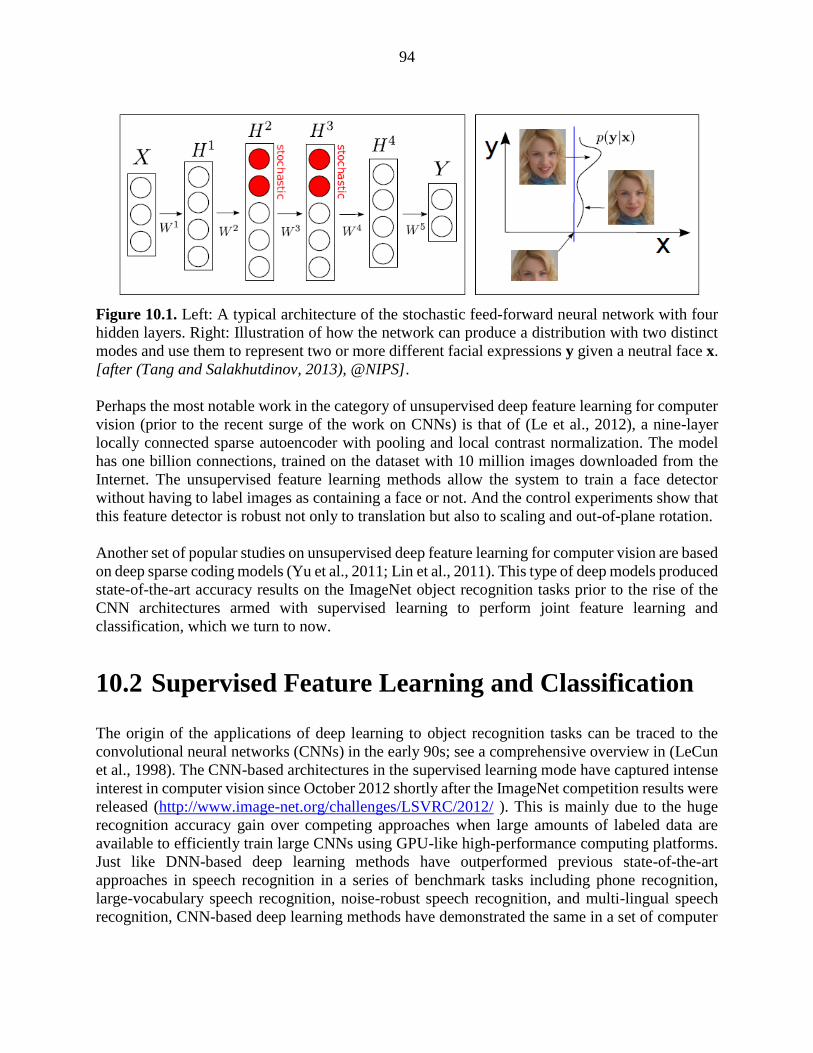
94

Figure 10.1. Left: A typical architecture of the stochastic feed-forward neural network with four

hidden layers. Right: Illustration of how the network can produce a distribution with two distinct

modes and use them to represent two or more different facial expressions y given a neutral face x.

[after (Tang and Salakhutdinov, 2013), @NIPS].

Perhaps the most notable work in the category of unsupervised deep feature learning for computer

vision (prior to the recent surge of the work on CNNs) is that of (Le et al., 2012), a nine-layer

locally connected sparse autoencoder with pooling and local contrast normalization. The model

has one billion connections, trained on the dataset with 10 million images downloaded from the

Internet. The unsupervised feature learning methods allow the system to train a face detector

without having to label images as containing a face or not. And the control experiments show that

this feature detector is robust not only to translation but also to scaling and out-of-plane rotation.

Another set of popular studies on unsupervised deep feature learning for computer vision are based

on deep sparse coding models (Yu et al., 2011; Lin et al., 2011). This type of deep models produced

state-of-the-art accuracy results on the ImageNet object recognition tasks prior to the rise of the

CNN architectures armed with supervised learning to perform joint feature learning and

classification, which we turn to now.

10.2 Supervised Feature Learning and Classification

The origin of the applications of deep learning to object recognition tasks can be traced to the

convolutional neural networks (CNNs) in the early 90s; see a comprehensive overview in (LeCun

et al., 1998). The CNN-based architectures in the supervised learning mode have captured intense

interest in computer vision since October 2012 shortly after the ImageNet competition results were

released (http://www.image-net.org/challenges/LSVRC/2012/ ). This is mainly due to the huge

recognition accuracy gain over competing approaches when large amounts of labeled data are

available to efficiently train large CNNs using GPU-like high-performance computing platforms.

Just like DNN-based deep learning methods have outperformed previous state-of-the-art

approaches in speech recognition in a series of benchmark tasks including phone recognition,

large-vocabulary speech recognition, noise-robust speech recognition, and multi-lingual speech

recognition, CNN-based deep learning methods have demonstrated the same in a set of computer

95

vision benchmark tasks including category-level object recognition, object detection, and semantic

segmentation.

The basic architecture of the CNN described in (LeCun et al., 1998) is shown in Figure 10.1. To

incorporate the relative invariance of the spatial relationship in typical image pixels with respect

to the location, the CNN uses a convolutional layer with local receptive fields and with tied filter

weights, much like 2-dimensional FIR filters in image processing. The output of the FIR filters is

then passed through a nonlinear activation function to create activation maps, followed by another

nonlinear pooling (labeled as “subsampling” in Figure 10.2) layer that reduces the data rate while

providing invariance to slightly different input images. The output of the pooling layer are subject

to a few fully-connected layers as in the DNN discussed in earlier chapters. The whole architecture

above is also called the deep CNN in the literature.

Figure 10.2. The original convolutional neural network that is composed of multiple alternating

convolution and pooling layers followed by fully connected layers. [after (LeCun, et al., 1998),

@IEEE].

Deep models with convolution structure such as CNNs have been found effective and have been

in use in computer vision and image recognition since 90’s (Bengio and LeCun, 1995; LeCun et

al., 1998; Jarrett et al., 2009; Kavukcuoglu et al., 2010; Ciresan et al., 2012; Krizhevsky et al.,

2012). The most notable advance was achieved in the 2012 ImageNet LSVRC competition, in

which the task is to train a model with 1.2 million high-resolution images to classify unseen images

to one of the 1000 different image classes. On the test set consisting of 150k images, the deep

CNN approach described in (Krizhevsky et al., 2012) achieved the error rates considerably lower

than the previous state-of-the-art. Very large deep-CNNs are used, consisting of 60 million weights,

and 650,000 neurons, and five convolutional layers together with max-pooling layers. Additional

two fully-connected layers as in the DNN described previously are used on top of the CNN layers.

Although all the above structures were developed separately in earlier work, their best combination

accounted for major part of the success. See the overall architecture of the deep CNN system in

Figure 10.3. Two additional factors contribute to the final success. The first is a powerful

regularization technique called “dropout”; see details in (Hinton et al., 2012a) and a series of

further analysis and improvement in (Baldi and Sadowski, 2013; McAllester, 2013; Frey and Ba,

2013; Wager et al., 2013). Applications of the same “dropout” techniques are also successful for

some speech recognition tasks (Deng et al., 2013; Dahl et al., 2013). The second factor is the use

of non-saturating neurons or rectified linear units (ReLU) that compute 𝑓(𝑥) = max(𝑥, 0), which

96

significantly speeds up the overall training process especially with efficient GPU implementation.

This deep-CNN system achieved a winning top-5 test error rate of 15.3% using extra training data

from ImageNet Fall 2011 release, or 16.4% using only supplied training data in ImageNet-2012,

significantly lower than 26.2% achieved by the second-best system which combines scores from

many classifiers using a set of hand-crafted features such as SIFT and Fisher vectors. See details

in http://www.image-net.org/challenges/LSVRC/2012/oxford_vgg.pdf about the best competing

method. It is noted, however, that the Fisher-vector-encoding approach has recently been extended

by Simonyan et al. (2013) via stacking in multiple layers to form deep Fisher networks, which

achieve competitive results with deep CNNs at a smaller computational learning cost.

Figure 10.3. The architecture of the deep-CNN system which won the 2012 ImageNet competition

by a large margin over the second-best system and the state of the art by 2012. [after (Krizhevsky

et al., 2012), @NIPS].

The state of the art performance demonstrated in (Krizhevsky et al., 2012) using the deep-CNN

approach is further improved by another significant margin during 2013, using a similar approach

but with bigger models and larger amounts of training data. A summary of top-5 test error rates

from 11 top-performing teams participating in the 2013 ImageNet ILSVRC competition is shown

in Figure 10.4, with the best result of the 2012 competition shown to the right most as the baseline.

Here we see rapid error reduction on the same task from the lowest pre-2012 error rate of 26.2%

(non-neural networks) to 15.3% in 2012 and further to 11.2% in 2013, both achieved with deep-

CNN technology. It is also interesting to observe that all major entries in the 2013 ImageNet

ILSVRC competition is based on deep learning approaches. For example, the Adobe system shown

in Figure 10.4 is based on the deep-CNN reported in (Krizhevsky et al., 2012) including the use

of dropout. The network architecture is modified to include more filters and connections. At test

time, image saliency is used to obtain 9 crops from original images, which are combined with the

standard five multiview crops. The NUS system uses a non-parametric, adaptive method to

combine the outputs from multiple shallow and deep experts, including deep-CNN, kernel, and

GMM methods. The VGG system is described in (Simonyan et al., 2013) and uses a combination

of the deep Fisher vector network and the deep-CNN. The ZF system is based on a combination

of a large CNN with a range of different architectures. The choice of architectures was assisted by

visualization of model features using a deconvolutional network as described by Zeiler et al. (2011),

97

Zeiler and Fergus (2013), and Zeiler (2014). The CognitiveVision system uses an image

classification scheme based on a DNN architecture. The method is inspired by cognitive

psychophysics about how the human vision system first learns to classify the basic-level categories

and then learns to classify categories at the subordinate level for fine-grained object recognition.

Finally, the best-performing system called Clarifai in Figure 10.4 is based on a large and deep

CNN with dropout regularization. It augments the amount of training data by down-sampling

images to 256 pixels. The system contains a total of 65M parameters. Multiple such models were

averaged together to further boost performance. The main novelty is to use the visualization

technique based on the deconvolutional networks as described in (Zeiler et. al, 2011; Zeiler,

2014) to identify what makes the deep model perform well, based on which a powerful deep

architecture was chosen. See more details of these systems in http://www.image-

net.org/challenges/LSVRC/2013/results.php .

Figure 10.4. Summary results of ImageNet Large Scale Visual Recognition Challenge 2013

(ILSVRC2013), representing the state-of-the-are performance of object recognition systems. Data

source: http://www.image-net.org/challenges/LSVRC/2013/results.php

While the deep CNN has demonstrated remarkable classification performance on object

recognition tasks, there has been no clear understanding of why they perform so well until recently.

Zeiler and Fergus (2013) conducted research to address just this issue, and then used the gained

understanding to further improve the CNN systems, which yielded excellent performance as shown

in Figure 10.4 with labels “ZF” and “Clarifai”. A novel visualization technique is developed that

gives insight into the function of intermediate feature layers of the deep CNN. The technique also

sheds light onto the operation of the full network acting as a classifier. The visualization technique

is based on a deconvolutional network, which maps the neural activities in intermediate layers of

98

the original convolutional network back to the input pixel space. This allows the researchers to

example what input pattern originally caused a given activation in the feature maps. Figure 10.5

(the top portion) illustrates how a deconvolutional network is attached to each of its layers, thereby

providing a closed loop back to image pixels as the input to the original CNN. The information

flow in this closed loop is as follows. First, an input image is presented to the deep CNN in a feed-

forward manner so that the features at all layers are computed. To examine a given CNN activation,

all other activations in the layer are set to zero and the feature maps are passed as input to the

attached deconvolutional network’s layer. Then, successive operations, opposite to the feed-

forward computation in the CNN, are carried out including unpooling, rectifying, and filtering.

This allows the reconstruction of the activity in the layer beneath that gave rise to the chosen

activation. These operations are repeated until input layer is reached. During unpooling, non-

invertibility of the max pooling operation in the CNN is resolved by an approximate inverse, where

the locations of the maxima within each pooling region are recorded in a set of “switch” variables.

These switches are used to place the reconstructions from the layer above into appropriate locations,

preserving the structure of the stimulus. This procedure is shown at the bottom portion of Figure

10.5.

In addition to the deep-CNN architecture described above, the DNN architecture has also been

shown to be highly successful in a number of computer vision tasks (Ciresan, et al., 2010, 2011,

2012, 2012a). We have not found in the literature on direct comparisons among the CNN, DNN,

and other related architectures on the identical tasks.

99

Figure 10.5. The top portion shows how a deconvolutional network’s layer (left) is attached to a

corresponding CNN’s layer (right). The deconvolutional network reconstructs an approximate

version of the CNN features from the layer below. The bottom portion is an illustration of the

unpooling operation in the deconvolutional network, where “Switches” are used to record the

location of the local max in each pooling region during pooling in the CNN. [after (Zeiler and

Fergus, 2013), @arXiv].

Finally, the most recent study on supervised learning for computer vision shows that the deep CNN

architecture is not only successful for object/image classification discussed earlier in this section

but also successful for objection detection in the whole images (Girshick et al., 2013). The

detection task is substantially more complex than the classification task.

As a brief summary of this chapter, deep learning has made huge inroads into computer vision,

soon after its success in speech recognition discussed in Chapter 7. So far, it is the supervised

learning paradigm based on the deep CNN architecture and the related classification techniques

that are making the greatest impact, showcased by the ImageNet competition results from 2012

100

and 2013. These methods can be used for not only objection recognition but also many other

computer vision tasks. There has been some debate as to the reasons for the success of these CNN-

based deep learning methods, and about their limitations. Many questions are still open as to how

these methods can be tailored to certain computer vision applications and how to scale up the

models and training data. Finally, we discussed a number of studies on unsupervised and

generative approaches of deep learning to computer vision and image modeling problems in the

earlier part of this chapter. Their performance has not been competitive with the supervised

learning approach on object recognition tasks with ample training data. To achieve long term and

ultimate success in computer vision, it is likely that unsupervised learning will be needed. To this

end, many open problems in unsupervised feature learning and deep learning need to be addressed

and much more research need to be carried out.

101

CHAPTER 11

SELECTED APPLICATIONS IN MULTI-

MODAL AND MULTI-TASK LEARNING

Multi-task learning is a machine learning approach that learns to solve several related problems at

the same time, using a shared representation. It can be regarded as one of the two major classes of

transfer learning or learning with knowledge transfer, which focuses on generalizations across

distributions, domains, or tasks. The other major class of transfer learning is adaptive learning,

where knowledge transfer is carried out in a sequential manner, typically from a source task to a

target task (Deng and Li, 2013). Multi-modal learning is a closely related concept to multi-task

learning, where the learning domains or “tasks” cut across several modalities for human-computer

interactions or other applications embracing a mixture of textual, audio/speech, touch, and visual

information sources.

The essence of deep learning is to automate the process of discovering effective features or

representations for any machine learning task, including automatically transferring knowledge

from one task to another concurrently. Multi-task learning is often applied to conditions where no

or very little training data are available for the target task domain, and hence is sometimes called

zero-shot or one-shot learning. It is evident that difficult multi-task leaning naturally fits the

paradigm of deep learning or representation learning where the shared representations and

statistical strengths across tasks (e.g., those involving separate modalities of audio, image, touch,

and text) is expected to greatly facilitate many machine learning scenarios under low- or zero-

resource conditions. Before deep learning methods were adopted, there had been numerous efforts

in multi-modal and multi-task learning. For example, a prototype called MiPad for multi-modal

interactions involving capturing, leaning, coordinating, and rendering a mix of speech, touch, and

visual information was developed and reported in (Huang et al., 2001; Deng et al., 2002). And in

(Zheng et al., 2004; Subramanya et al., 2005), mixed sources of information from multiple-sensory

microphones with separate bone-conductive and air-born paths were exploited to de-noise speech.

These early studies all used shallow models and learning methods and achieved worse than desired

performance. With the advent of deep learning, it is hopeful that the difficult multi-modal learning

problems can be solved with eventual success to enable a wide range of practical applications. In

this chapter, we will review selected applications in this area, organized according to different

combinations of more than one modalities or learning tasks. Much of the work reviewed here is

on-going research, and readers should expect follow-up publications in the future.

11.1 Multi-Modalities: Text and Image

The underlying mechanism for potential effectiveness of multi-modal learning involving text and

image is the common semantics associated with the text and image. The relationship between the

102

text and image may come, for example, from the text annotations of an image (as the training data

for a multi-modal learning system). If the related text and image share the same representation in

a common semantic space, the system can generalize to the unseen situation where either text or

image is unavailable. It can thus be naturally used for zero-shot learning for image or text. In other

words, multi-modality learning can use text information to help image/visual recognition, and vice

versa. Exploiting text information for image/visual recognition constitutes most of the work done

in this space, which we review in this section below.

The deep architecture, called DeViSE (Deep Visual-Semantic Embedding) and developed by

Frome et al. (2013), is a typical example of the multi-modal learning where text information is

used to improve the image recognition system, especially for performing zero-shot learning. Image

recognition systems are often limited in their ability to scale to large number of object categories,

due in part to the increasing difficulty of acquiring sufficient training data with text labels as the

number of image categories grows. The multi-modal DeViSE system is aimed to leverage text data

to train the image models. The joint model is trained to identify image classes using both labeled

image data and the semantic information learned from unannotated text. An illustration of the

DeViSE architecture is shown in the center portion of Figure 10.1. It is initialized with the

parameters pre-trained at the lower layers of two models: the deep-CNN for image classification

in the left portion of the figure and the text embedding model in the right portion of the figure. The

part of the deep CNN, labeled “core visual model” in Figure 10.1, is further learned to predict the

target word-embedding vector using a projection layer labeled “transformation” and using a

similarity metric. The loss function used in training adopts a combination of dot-product similarity

and max-margin, hinge rank loss. The former is the un-normalized version of the cosine loss

function used for training the DSSM model in (Huang et al., 2013) as described in Chapter 9.3.

The latter is similar to the earlier joint image-text model called WSABIE (Web Scale Annotation

by Image Embedding developed by Weston, et al. (2010, 2011)). The results show that the

information provided by text improves zero-shot image predictions, achieving good hit rates (close

to 15%) across thousands of the labels never seen by the image model.

Figure 11.1. Illustration of the multi-modal DeViSE architecture. The left portion is an image

recognition neural network with a softmax output layer. The right portion is a skip-gram text model

103

providing word embedding vectors; see Chapter 8.2 and Figure 8.3 for details. The center is the

joint deep image-text model of DeViSE, with the two Siamese branches initialized by the image

and word embedding models below the softmax layers. The layer labeled “transformation” is

responsible for mapping the outputs of the image (left) and text (right) branches into the same

semantic space. [after (Frome, et al., 2013), @NIPS].

The earlier WSABIE system as described in (Weston, et al. 2010, 2011) adopted a shallow

architecture and trained a joint embedding model of both images and labels. Rather than using

deep architectures to derive the highly nonlinear image (as well as text-embedding) feature vectors

as in DeViSE, the WSABIE uses simple image features and a linear mapping to arrive at the joint

embedding space. Further, it uses an embedding vector for each possible label. Thus, unlike

DeViSE, WSABIE could not generalize to new classes.

It is also interesting to compare the DeViSE architecture of Figure 11.1 with the DSSM

architecture of Figure 9.2 in Chapter 9. The branches of “Query” and “Documents” in DSSM are

analogous to the branches of “image” and “text-label” in DeViSE. Both DeViSE and DSSM use

the objective function related to cosine distance between two vectors for training the network

weights in an end-to-end fashion. One key difference, however, is that the two sets of inputs to the

DSSM are both text (i.e., “Query” and “Documents” designed for IR), and thus mapping “Query”

and “Documents” to the same semantic space is conceptually more straightforward compared with

the need in DeViSE for mapping from one modality (image) to another (text). Another key

difference is that the generalization ability of DeViSE to unseen image classes comes from

computing text embedding vectors for many unsupervised text sources (i.e., with no image

counterparts) that would cover the text labels corresponding to the unseen classes. The

generalization ability of the DSSM over unseen words, however, is derived from a special coding

scheme for words in terms of their constituent letters.

The DeViSE architecture has inspired a more recent method, which maps images into the semantic

embedding space via convex combination of embedding vectors for the text label and the image

classes (Norouzi et al., 2013). Here is the main difference. DeViSE replaces the last, softmax layer

of a CNN image classifier with a linear transformation layer. The new transformation layer is then

trained together with the lower layers of the CNN. The method in (Norouzi et al., 2013) is much

simpler --- keeping the softmax layer of the CNN while not training the CNN. For a test image,

the CNN first produces top N-best candidates. Then, the convex combination of the corresponding

N embedding vectors in the semantic space is computed. This gives a deterministic transformation

from the outputs of the softmax classifier into the embedding space. This simple multi-modal

learning method is shown to work very well on the ImageNet zero-shot learning task.

Another thread of studies separate from but related to the above work on multi-modal learning

involving text and image have centered on the use of multi-modal embeddings, where data from

multiple sources with separate modalities of text and image are projected into the same vector

space. For example, Socher and Fei-Fei (2010) project words and images into the same space using

kernelized canonical correlation analysis. Socher et al. (2013b) map images to single-word vectors

so that the constructed multi-modal system can classify images without seeing any examples of

the class, i.e., zero-shot learning similar to the capability of DeViSE. The most recent work by

Socher et al. (2013c) extends their earlier work from single-word embeddings to those of phrases

104

and full-length sentences. The mechanism for mapping sentences instead of the earlier single

words into the multi-modal embedding space is derived from the power of the recursive neural

network described in Socher et al. (2013a) as summarized in Chapter 8.2, and its extension with

dependency tree.

In addition to mapping text to image (or vice versa) into the same vector space or to creating the

joint image/text embedding space, multi-modal learning for text and image can also be cast in the

framework of language models. In (Kiros, et al., 2013), a model of natural language is made

conditioned on other modalities such as image as the focus of the study. This type of multi-modal

language model is used to 1) retrieve images given complex description queries, 2) retrieve phrase

descriptions given image queries, and 3) generate text conditioned on images. Word

representations and image features are jointly learned by training the multi-modal language model

together with a convolutional network. An illustration of the multi-modal language model is shown

in Figure 11.2.

Figure 11.2. A multi-modal language model (of the type of log-bilinear) which predicts a word

conditioned not only on the previous words in the sentence but also on images. The model operates

on word embedding vectors. [after (Kiros et al., 2013), @NIPS].

11.2 Multi-Modalities: Speech and Image Ngiam et al. (2011) propose and evaluate an application of deep networks to learn features over

audio/speech and image/video modalities. They demonstrate cross-modality feature learning,

where better features for one modality (e.g., image) is learned when multiple modalities (e.g.,

speech and image) are present at feature learning time. A bi-modal deep autoencoder architecture

for separate audio/speech and video/image input channels are shown in Figure 11.3. The essence

of this architecture is to use a shared, middle layer to represent both types of modalities. This is a

straightforward generalization from the single-modal deep autoencoder for speech shown in Figure

4.1 of Chapter 4 to bi-modal counterpart. The authors further show how to learn a shared audio

and video representation, and evaluate it on a fixed task, where the classifier is trained with audio-

only data but tested with video-only data and vice versa. The work concludes that deep learning

105

architectures are generally effective in learning multimodal features from unlabeled data and in

improving single modality features through cross modality information transfer. One exception is

the cross-modality setting using the CUAVE dataset. The results presented in (Ngiam et al., 2011)

show that learning video features with both video and audio outperforms that with only video data.

However, the same paper also shows that a model of (Papandreou, 2009) in which a sophisticated

signal processing technique for extracting visual features, together with the uncertainty-

compensation method developed originally from robust speech recognition (Deng et al., 2005),

gives the best classification accuracy in the cross-modal learning task, beating the features derived

from the generative deep architecture designed for this task.

Figure 11.3. The architecture of a deep denoising autoencoder for multi-modal audio/speech and

visual features. [after (Ngiam et al., 2011), @ICML].

While the deep generative architecture for multimodal learning described in (Ngiam et al., 2011)

is based on non-probabilistic autoencoder neural nets, a probabilistic version based on deep

Boltzmann machine (DBM) has appeared more recently for the same multimodal application. In

(Srivastava and Salakhutdinov, 2012), a DBM is used to extract a unified representation integrating

separate modalities, useful for both classification and information retrieval tasks. Rather than using

the “bottleneck” layers in the deep autoencoder to represent multimodal inputs, here a probability

density is defined on the joint space of multimodal inputs, and states of suitably defined latent

variables are used for the representation. The advantage of this probabilistic formulation, possibly

lacking in the traditional deep autoencoder, is that the missing modality’s information can be filled

in naturally by sampling from its conditional distribution. More recent work on autoencoders

(Bengio et al., 2013, 2013b) shows the capability of generalized denoising autoencoders in

carrying out sampling, thus they may overcome the earlier problem of filling-in the missing

modality’s information. For the bi-modal data consisting of image and text, the multimodal DBM

106

was shown to slightly outperform the traditional version of the deep multimodal autoencoder as

well as multimodal DBN in classification and information retrieval tasks. No results on the

comparisons with the generalized version of deep autoencoders has been reported but may appear

soon.

The several architectures discussed so far in this chapter for multi-modal processing and learning

can be regarded as special cases of more general multi-task learning and transfer learning (Caruana,

1997; Bengio et al., 2013). Transfer learning, encompassing both adaptive and multi-task learning,

refers to the ability of a learning architecture and technique to exploit common hidden explanatory

factors among different learning tasks. Such exploitation permits sharing of aspects of diverse

types of input data sets, thus allowing the possibility of transferring knowledge across seemingly

different learning tasks. As argued in (Bengio et al., 2013), the learning architecture shown in

Figure 11.4 and the associated learning algorithms have an advantage for such tasks because they

learn representations that capture underlying factors, a subset of which may be relevant for each

particular task. We will discuss a number of such multi-task learning applications in the remainder

of this chapter that are confined with a single modality of speech, natural language processing, or

image domain.

Figure 11.4. A DNN architecture for multitask learning that is aimed to discover hidden

explanatory factors shared among three tasks A, B, and C. [after (Bengio, 2013), @IEEE].

11.3 Multi-Task Learning within the Speech, NLP or

Image Domain

Within the speech domain, one most interesting application of multi-task learning is multi-lingual

or cross-lingual speech recognition, where speech recognition for different languages is considered

as different tasks. Various approaches have been taken to attack this rather challenging acoustic

modeling problem for speech recognition, where the difficulty lies in the lack of transcribed speech

data due to economic considerations in developing speech recognition systems for all languages

in the world. Cross-language data sharing and data weighing are common and useful approaches

for the GMM-HMM system (Lin et al., 2009). Another successful approach for the GMM-HMM

107

is to map pronunciation units across languages either via knowledge-based or data-driven methods

(Yu et al., 2009b). But they are much inferior to the DNN-HMM approach which we now

summarize.

In recent papers of (Huang et al., 2013; Deng et al., 2013a) and (Heigold et al., 2013), two research

groups independently developed closely related DNN architectures with multi-task learning

capabilities for multilingual speech recognition. See Figure 11.5 for an illustration of this type of

architecture. The idea behind these architectures is that the hidden layers in the DNN, when learned

appropriately, serve as increasingly complex feature transformations sharing common hidden

factors across the acoustic data in different languages. The final softmax layer representing a log-

linear classifier makes use of the most abstract feature vectors represented in the top-most hidden

layer. While the log-linear classifier is necessarily separate for different languages, the feature

transformations can be shared across languages. Excellent multilingual speech recognition results

are reported, far exceeding the earlier results using the GMM-HMM based approaches (e.g., Lin

et al., 2009; Yu et al., 2009b). The implication of this set of work is significant and far reaching.

It points to the possibility of quickly building a high-performance DNN-based system for a new

language from an existing multilingual DNN. This huge benefit would require only a small amount

of training data from the target language, although having more data would further improve the

performance. This multitask learning approach can reduce the need for the unsupervised pre-

training stage, and can train the DNN with much fewer epochs. Extension of this set of work would

be to efficiently build a language-universal speech recognition system. Such a system cannot only

recognize many languages and improve the accuracy for each individual language, but also expand

the languages supported by simply stacking softmax layers on the DNN for new languages.

Figure 11.5. A DNN architecture for multilingual speech recognition. [after (Huang et al., 2013),

@IEEE].

108

A closely related DNN architecture, as shown in Figure 11.6, with multitask learning capabilities

was also recently applied to another acoustic modeling problem --- learning joint representations

for two separate sets of acoustic data (Li et al., 2012; Deng et al., 2013a). The set that consists of

the speech data with 16kHz sampling rate is of wideband and high quality, which is often collected

from increasingly popular smart phones under the voice search scenario. Another, narrowband

data set has a lower sampling rate of 8kHz, often collected using the telephony speech recognition

systems.

Figure 11.6. A DNN architecture for speech recognition trained with mixed-bandwidth acoustic

data with 16-kHz and 8-kHz sampling rates; [after (Li et al., 2012), @IEEE].

As a final example of multi-task learning within the speech domain, let us consider phone

recognition and word recognition as separate “tasks”. That is, phone recognition results are used

not for producing text outputs but for language-type identification or for spoken document retrieval.

Then, the use of pronunciation dictionary in almost all speech systems can be considered as multi-

task learning that share the tasks of phone recognition and word recognition. More advanced

frameworks in speech recognition have pushed this direction further by advocating the use of even

finer units of speech than phones to bridge the raw acoustic information of speech to semantic

content of speech via a hierarchy of linguistic structure. These atomic speech units include “speech

attributes” in the detection-based and knowledge-rich modeling framework for speech recognition,

whose accuracy has been significantly boosted recently by the use of deep learning methods (Yu

et al., 2012a; Siniscalchi et al., 2013, 2013a).

Within the natural language processing domain, the best known example of multi-task learning is

the comprehensive studies reported in (Collobert and Weston, 2008; Collobert et al., 2011), where

a range of separate “tasks” of part-of-speech tagging, chunking, named entity tagging, semantic

role identification, and similar-word identification in natural language processing are attacked

109

using a common representation of words and a unified deep learning approach. A summary of

these studies can be found in Chapter 8.2.

Finally, within the domain of image/vision as a single modality, deep learning has also been found

effective in multi-task learning. Srivastava and Salakhutdinov (2013) present a multi-task learning

approach based on hierarchical Bayesian priors in a DNN system applied to various image

classification data sets. The priors are combined with a DNN, which improves discriminative

learning by encouraging information sharing among tasks and by discovering similar classes

among which knowledge is transferred. More specifically, methods are developed to jointly learn

to classify images and a hierarchy of classes, such that “poor classes”, for which there are relatively

few training examples, can benefit from similar “rich classes”, for which more training examples

are available. This work can be considered as an excellent instance of learning output

representations, in addition to learning input representation of the DNN as the focus of nearly all

deep learning work reported in the literature.

As another example of multi-task learning within the single-modality domain of image, Ciresan et

al. (2012b) applied the architecture of deep CNNs to character recognition tasks for Latin and for

Chinese. The deep CNNs trained on Chinese characters are shown to be easily capable of

recognizing uppercase Latin letters. Further, learning Chinese characters is accelerated by first pre-

training a CNN on a small subset of all classes and then continuing to train on all classes.

110

CHAPTER 12

EPILOGUES

This book first presented a brief history of deep learning (focusing on speech recognition) and

developed a categorization scheme to analyze the existing deep networks in the literature into

unsupervised (many of which are generative), supervised, and hybrid classes. The deep

autoencoder, the DSN (as well as many of its variants), and the DBN-DNN or pre-trained DNN

architectures, one in each of the three classes, are discussed and analyzed in detail, as they appear

to be popular and promising approaches based on the authors’ personal research experiences.

Applications of deep learning in five broad areas of information processing are also reviewed,

including speech and audio (Chapter 7), natural language modeling and processing (Chapter 8),

information retrieval (Chapter 9), object recognition and computer vision (Chapter 10), and multi-

modal and multi-task learning (Chapter 11). There are other interesting yet non-mainstream

applications of deep learning, which are not covered in this book. For interested readers, please

consult recent papers on the applications of deep learning to optimal control in (Levine, 2013), to

reinforcement learning in (Mnih, et al, 2013), to malware classification in (Dahl et al., 2013a), to

compressed sensing in (Palangi et al., 2013), to recognition confidence prediction in (Huang et al.,

2013a), to acoustic-articulatory inversion mapping in (Uria et al., 2011), to emotion recognition

from video in (Kahou et al., 2013), to emotion recognition from speech in (Li et al., 2013; Le and

Mower, 2013), to spoken language understanding in (Mesnil et al., 2013; Yao et al., 2013; Tur et

al., 2012), to speaker recognition in (Vasilakakis et al., 2013; Stafylakis et al., 2012), to language-

type recognition in (Diez, 2013), to dialogue state tracking for spoken dialogue systems in

(Henderson et al., 2013; Deng et al., 2013a), to automatic voice activity detection in (Zhang and

Wu, 2013), to speech enhancement in (Xu et al., 2014), to voice conversion in (Nakashika et al.,

2013), and to single-channel source separation in (Grais et al., 2013; Weng et al.. 2014).

The literature on deep learning is vast, mostly coming from the machine learning community. The

signal processing community embraced deep learning only within the past four years or so (starting

around end of 2009) and the momentum is growing fast ever since. This book is written mainly

from the signal processing perspective. Beyond just surveying the existing deep learning work, a

classificatory scheme based on the architectures and on the nature of the learning algorithms is

developed, and an analysis and discussion with concrete examples are presented. This will

hopefully provide insight for readers to better understand the capability of the various deep

learning systems discussed in the book, the connection among different but similar deep learning

methods, and how to design proper deep learning algorithms under different circumstances.

Throughout this review, the important message is conveyed that building and learning deep

hierarchies of features are highly desirable. We have discussed the difficulty of learning

parameters in all layers of deep networks in one shot due to optimization difficulties that need to

be better understood. The unsupervised pre-training method in the hybrid architecture of the DBN-

DNN, which we reviewed in detail in Chapter 5, appears to have offered a useful, albeit empirical,

solution to poor local optima in optimization and to regularization for the deep model containing

111

massive parameters even though a solid theoretical foundation is still lacking. The effectiveness

of the pre-training method, which was one factor stimulating the interest in deep learning by the

signal processing community in 2009 via collaborations between academic and industrial

researchers, is most prominent when the supervised training data are limited.

Deep learning is an emerging technology. Despite the empirical promising results reported so far,

much more work needs to be carried out. Importantly, it has not been the experience of deep

learning researchers that a single deep learning technique can be successful for all classification

tasks. For example, while the popular learning strategy of generative pre-training followed by

discriminative fine-tuning seems to work well empirically for many tasks, it failed to work for

some other tasks that have been explored (e.g., language identification or speaker recognition;

unpublished by the authors of this book). For these tasks, the features extracted at the generative

pre-training phase seem to describe the underlying speech variations well but do not contain

sufficient information to distinguish between different languages. A learning strategy that can

extract discriminative yet also invariant features is expected to provide better solutions. This idea

has also been called “disentangling” and is developed further in (Bengio et al., 2013a). Further,

extracting discriminative features may greatly reduce the model size needed in many of the current

deep learning systems. Domain knowledge such as what kind of invariance is useful for a specific

task in hand (e.g., vision, speech, or natural language) and what kind of regularization in terms of

parameter constraints is key to the success of applying deep learning methods. Moreover, new

types of DNN architectures and learning beyond the several popular ones discussed in this book

are currently under active development by the deep learning research community (e.g., Bengio et

al., 2013a; Deng et al., 2013b), holding the promise to improve the performance of deep learning

models in more challenging applications in signal processing and in artificial intelligence.

Recent published work showed that there is vast room to improve the current optimization

techniques for learning deep architectures (Martens, 2010; Le et al., 2011; Martens and Sutskever,

2011; Dean et al., 2012; Sutskever, 2013; Sainath et al., 2013; Wright et al., 2013). To what extent

pre-training is essential to learning the full set of parameters in deep architectures is currently

under investigation, especially when very large amounts of labeled training data are available,

reducing or even obliterating the need for model regularization. Some preliminary results have

been discussed in this book and in (Ciresan et al., 2010; Yu et al. 2010; Seide et al. 2011; Hinton

et al., 2012).

In recent years, machine learning is becoming increasingly dependent on large-scale data sets. For

instance, many of the recent successes of deep learning as discussed in this book have relied on

the access to massive data sets and massive computing power. It would become increasingly

difficult to explore the new algorithmic space without the access to large, real-world data sets and

without the related engineering expertise. How well deep learning algorithms behave would

depend heavily on the amount of data and computing power available. As we showed with speech

recognition examples, a deep learning algorithm that appears to be performing not so remarkably

on small data sets can begin to perform considerably better when these limitations are removed,

one of main reasons for the recent resurgence in neural network research. As an example, the DBN

pre-training that ignited a new era of (deep) machine learning research appears unnecessary if

enough data and computing power are used.

112

As a consequence, effective and scalable parallel algorithms are critical for training deep models

with large data sets, as in many common information processing applications such as speech

recognition and machine translation. The popular mini-batch stochastic gradient technique is

known to be difficult to parallelize over computers. The common practice nowadays is to use

GPGPUs to speed up the learning process, although recent advance in developing asynchronous

stochastic gradient descent learning has shown promises by using large-scale CPU clusters (e.g.

Le et al., 2012; Dean et al., 2012) and GPU clusters (Coates et al., 2013). In this interesting

computing architecture, many different replicas of the DNN compute gradients on different subsets

of the training data in parallel. These gradients are communicated to a central parameter server

that updates the shared weights. Even though each replica typically computes gradients using

parameter values not immediately updated, stochastic gradient descent is robust to the slight errors

this has introduced. To make deep learning techniques scalable to very large training data,

theoretically sound parallel learning and optimization algorithms together with novel architectures

need to be further developed (e.g., Bottou and LeCun, 2004; Chen et al., 2012; Seide et al., 2014;

Dean et al., 2012; Hutchinson et al., 2013; Sutskever, 2013; Bengio et al., 2013). Optimization

methods specific to speech recognition problems may need to be taken into account in order to

push speech recognition advances to the next level (e.g., Wright et al., 2013; Cardinal et al., 2013;

Heigold et al., 2013a).

One major barrier to the application of DNNs and related deep models is that it currently requires

considerable skill and experience to choose sensible values for hyper-parameters such as the

learning rate schedule, the strength of the regularizer, the number of layers and the number of units

per layer, etc. Sensible values for one hyper-parameter may depend on the values chosen for other

hyper-parameters and hyper-parameter tuning in DNNs is especially expensive. Some interesting

methods for solving the problem have been developed recently, including random sampling

(Bergstra et al., 2012) and Bayesian optimization procedure (Snoek et al., 2012). Further research

is needed in this important area.

This book, mainly in Chapters 8 and 11 on natural language and multi-modal applications, has

touched on some recent work on using deep learning methods to do reasoning, moving beyond the

topic of more straightforward pattern recognition using supervised, unsupervised or hybrid

learning methods to which much of this book has been devoted to. In principle, since deep

networks are naturally equipped with distributed representations (rf. Table 3.1) using their layer-

wise collections of units for coding relations and coding entities, concepts, events, topics, etc., they

can potentially perform powerful reasoning over structures, as argued in various historical

publications as well as recent essays (e.g., Hinton, 1990; Smolensky, 1990; Pollack, 1990; Plate,

1995; Prince and Smolensky, 1997; Bottou, 2013). While initial explorations on this capability of

deep networks have recently appeared in the literature, as reviewed in Chapters 8 and 11, much

research is needed. If successful, this new type of deep learning “machine” will open up many

novel and exciting applications in applied artificial intelligence as a “thinking brain”. We expect

growing work of deep learning in this area, full of new challenges, in the future.

Further, solid theoretical foundations of deep learning need to be established in a myriad of aspects.

As an example, the success of deep learning in unsupervised learning has not been demonstrated

as much as for supervised learning; yet the essence and major motivation of deep learning lie right

in unsupervised learning for automatically discovering data representation. The issues involve

113

appropriate objectives for learning effective feature representations and the right deep learning

architectures/algorithms for distributed representations to effectively disentangle the hidden

explanatory factors of variation in the data. Unfortunately, a majority of the successful deep

learning techniques have so far dealt with unstructured or “flat” classification problems. For

example, although speech recognition is a sequential classification problem by nature, in the most

successful and large-scale systems, a separate HMM is used to handle the sequence structure and

the DNN is only used to produce the frame-level, unstructured posterior distributions. Recent

proposals have called for and investigated moving beyond the “flat” representations and

incorporating structures in both the deep learning architectures and input and output

representations (Socher, 2012; Deng, 2013; Srivastava and Salakhutdinov, 2013; Graves et al.,

2013).

Finally, deep learning researchers have been advised by neuroscientists to seriously consider a

broader set of issues and learning architectures so as to gain insight into biologically plausible

representations in the brain that may be useful for practical applications (e.g., Olshausen, 2012).

How can computational neuroscience models about hierarchical brain structure help improve

engineering deep learning architectures? How may the biologically feasible learning styles in the

brain (e.g., Hinton, 2003; Xie and Seung, 2003) help design more effective and more robust deep

learning algorithms? All these issues and those discussed in this chapter will need intensive

research in order to further push the frontier of deep learning.

114

BIBLIOGRAPHY

Abdel-Hamid, O., Mohamed, A., Jiang, H., and G. Penn, “Applying convolutional neural networks

concepts to hybrid NN-HMM model for speech recognition,” Proc. ICASSP, 2012.

Abdel-Hamid, O., Deng, L., and Yu. D. “Exploring convolutional neural network structures and

optimization for speech recognition,” Interspeech, 2013.

Abdel-Hamid, O., Deng, L., Yu. D., Jiang, H. “Deep segmental neural networks for speech

recognition,” Proc. Interspeech, 2013a.

Acero, A., Deng, L., Kristjansson, T., and Zhang, J. “HMM adaptation using vector Taylor series

for noisy speech recognition,” Proc. Interspeech, 2000.

Alain, G. and Bengio, Y. “What Regularized Autoencoders Learn from the Data Generating

Distribution,” Proc. International Conference on Learning Representations (ICLR), 2013.

Anthes, G. “Deep learning comes of age,” Communications of the ACM, Vol. 56 No. 6, pp. 13-

15, June 2013.

Arel, I., Rose, C., and Karnowski, T. “Deep Machine Learning - A New Frontier in Artificial

Intelligence,” IEEE Computational Intelligence Mag., vol. 5, pp. 13-18, November, 2010.

Aslan, O., Cheng, H., Schuurmans, D., and Zhang, X. “Convex two-layer modeling,” Proc. NIPS,

2013.

Ba, J. and Frey, B. “Adaptive dropout for training deep neural networks,” Proc. NIPS, 2013.

Baker, J., Deng, L., Glass, J., Khudanpur, S., Lee, C.-H., Morgan, N., and O’Shaughnessy, D.

“Research developments and directions in speech recognition and understanding,” IEEE Sig.

Proc. Mag., vol. 26, no. 3, May 2009, pp. 75-80.

Baker, J., Deng, L., Glass, J., Khudanpur, S., Lee, C.-H., Morgan, N., and O’Shaughnessy, D.

“Updated MINS report on speech recognition and understanding,” IEEE Sig. Proc. Mag., vol.

26, no. 4, July 2009a.

Baldi, P. and Sadowski, P. “Understanding Dropout,” Proc. NIPS, 2013.

Battenberg, E., Schmidt, E., and Bello, J. Deep learning for music, special session at ICASSP

(http://www.icassp2014.org/special_sections.html#SS8), 2014.

Batternberg, E. and Wessel, D. “Analyzing drum patterns using conditional deep belief networks,”

Proc. ISMIR, 2012.

Bell, P., Swietojanski, P., and Renals, S. “Multi-level adaptive networks in tandem and hybrid

ASR systems”, Proc. ICASSP, 2013.

Bengio, Y., Yao, L., Alain, G., and Vincent, P. “Generalized denoising autoencoders as generative

models,” Proc. NIPS, 2013.

Bengio, Y. “Deep learning of representations: Looking forward,” in: Statistical Language and

Speech Processing, pp. 1--37, Springer, 2013.

Bengio, Y., Boulanger, N., and Pascanu, R. “Advances in optimizing recurrent networks,” Proc.

ICASSP, 2013.

Bengio, Y., Courville, A., and Vincent, P. “Representation learning: A review and new

perspectives,” IEEE Trans. PAMI, vol. 38, pp. 1798-1828, 2013a.

Bengio, Y., Thibodeau-Laufer, E., and Yosinski, J. “Deep generative stochastic networks trainable

by backprop,” arXiv 1306:1091, 2013b.

Bengio, Y. “Deep Learning of Representations for Unsupervised and Transfer Learning,” JMLR

Workshop and Conference Proceedings, vol. 27, pp. 17-37, 2012.

115

Bengio, Y. “Learning deep architectures for AI,” in Foundations and Trends in Machine Learning,

Vol. 2, No. 1, 2009, pp. 1-127.

Bengio, Y., Lamblin, P., Popovici, D., and Larochelle, H. “Greedy Layer-Wise Training of Deep

Networks,” Proc. NIPS, 2006.

Bengio, Y., Ducharme, R., Vincent, P., and Jauvin, C. “A Neural Probabilistic Language Model,”

Journal of Machine Learning Research, vol. 3, pp. 1137-1155, 2003.

Bengio, Y., Ducharme, R., Vincent, P. and Jauvin, C. “A neural probabilistic language model,”

Proc. NIPS, 2000.

Bengio, Y., De Mori, R., Flammia, G., and Kompe, R. “Global Optimization of a Neural Network-

Hidden Markov Model Hybrid,” IEEE Transactions on Neural Networks, vol. 3, pp. 252-259,

1992.

Bengio, Y. Artificial Neural Networks and Their Application to Sequence Recognition, Ph.D.

Thesis, McGill University, Montreal, Canada, 1991.

Bergstra, J. and Bengio, Y. “Random search for hyper-parameter optimization,” J. Machine

Learning Research,” Vol. 3, pp. 281-305, 2012.

Bottou, L. and LeCun. Y. “Large scale online learning,” Proc. NIPS, 2004.

Bilmes, J. “Dynamic graphical models,” IEEE Signal Processing Mag., vol. 33, pp. 29–42, 2010.

Bilmes, J. and Bartels, C. “Graphical model architectures for speech recognition,” IEEE Signal

Processing Mag., vol. 22, pp. 89–100, 2005.

Bordes, A., Weston, J., Collobert, R., and Bengio, Y. “Learning Structured Embeddings of

Knowledge Bases,” Proc. AAAI, 2011.

Bordes, A., Weston, J., Collobert, R., and Bengio, Y. “Learning Structured Embeddings of

Knowledge Bases,” Proc. AAAI, 2011.

Bordes, A., Glorot, X., Weston, J., and Bengio, Y. “A semantic matching energy function for learning with multi-relational data --- Application to word-sense disambiguation,” Machine

Learning, May, 2013.

Boulanger-Lewandowski, N., Bengio, Y., and Vincent, P. “Audio Chord Recognition with

Recurrent Neural Networks,” Proc. ISMIR, 2013.

Bourlard, H. and Morgan, N., Connectionist Speech Recognition: A Hybrid Approach, Norwell,

MA: Kluwer, 1993.

Bottou, L. “From machine learning to machine reasoning: an essay,” Journal of Machine Learning

Research, Vol. 14, pp. 3207-3260, 2013.

Bouvrie, J. “Hierarchical Learning: Theory with Applications in Speech and Vision,” Ph.D. thesis,

MIT, 2009.

Bridle, J., Deng, L., Picone, J., Richards, H., Ma, J., Kamm, T., Schuster, M., Pike, S., and Reagan,

R. “An investigation of segmental hidden dynamic models of speech coarticulation for

automatic speech recognition,” Final Report for 1998 Workshop on Language Engineering,

CLSP, Johns Hopkins, 1998.

Cardinal, P.; Dumouchel, P.; Boulianne, G., "Large Vocabulary Speech Recognition on Parallel

Architectures," IEEE Transactions on Audio, Speech, and Language Processing, vol.21, no.11,

pp.2290,2300, Nov. 2013.

Caruana, R. “Multitask Learning,” Machine Learning, Vol. 28, pp. 41-75, 1997.

Chen, J. and Deng, L. “A Primal-Dual Method for Training Recurrent Neural Networks

Constrained by the Echo-State Property”, arXiv:1311.6091, pp. 1-16, 2013.

Chen, X., Eversole, A., Li, G., Yu, D. and Seide, F., “Pipelined Back-Propagation for Context-

Dependent Deep Neural Networks”, Proc. Interspeech 2012.

116

Chengalvarayan, R. and Deng, L. “Speech Trajectory Discrimination using the Minimum

Classification Error Learning,” IEEE Transactions on Speech and Audio Processing, vol. 6,

no. 6, pp. 505-515, 1998.

Chengalvarayan R. and Deng, L. “HMM-based speech recognition using state-dependent,

discriminatively derived transforms on Mel-warped DFT features,” IEEE Transactions on

Speech and Audio Processing, pp. 243-256, 1997.

Chengalvarayan R. and Deng, L. “Use of generalized dynamic feature parameters for speech

recognition,” IEEE Transactions on Speech and Audio Processing, pp. 232-242, 1997a.

Cho, Y. and Saul, L. “Kernel methods for deep learning,” Proc. NIPS, pp. 342–350, 2009.

Ciresan, D., Meier, U., and Schmidhuber, J. “Multi-column deep neural networks for image

classification.” Proc. CVPR, 2012.

Ciresan, D., Giusti, A., Gambardella, L., and Schmidhuber, J. “Deep neural networks segment

neuronal membranes in electron microscopy images,” Proc. NIPS, 2012a.

Ciresan, D. C., Meier, U., & Schmidhuber, J. “Transfer learning for Latin and Chinese characters

with deep neural networks,” Proc. IJCNN, 2012b.

Ciresan, D., Meier, U., Masci, J., and Schmidhuber, J. “A committee of neural networks for traffic

sign classification,” Proc. IJCNN, 2011.

Ciresan, D., Meier, U., Gambardella, L., and Schmidhuber, J. “Deep, Big, Simple Neural Nets for

Handwritten Digit Recognition,” Neural Computation, December 2010.

Coates, A., Huval, B., Wang, T., Wu, D., Ng, A., and Catanzaro, B. “Deep Learning with COTS

HPC,” Proc. ICML, 2013.

Cohen, W. and R. V. de Carvalho. “Stacked sequential learning,” Proc. IJCAI, pp. 671–676, 2005.

Collobert, R. “Deep learning for efficient discriminative parsing,” Proc. AISTATS, 2011.

Collobert, R. and Weston J. “A unified architecture for natural language processing: Deep neural

networks with multitask learning,” Proc. ICML, 2008.

Collobert, R., Weston, J., Bottou, L., Karlen, M., Kavukcuoglu, K., and Kuksa, P. “Natural

language processing (almost) from scratch,” J. Machine Learning Research, Vo. 12, pp. 2493-

2537, 2011.

Dahl, G, Sainath, T., and Hinton, G. “Improving deep neural networks for LVCSR using rectified

linear units and dropout,” Proc. ICASSP, 2013.

Dahl, G., Stokes, J., Deng, L., and Yu, D. “Large-Scale Malware Classification Using Random

Projections and Neural Networks,” Proc. ICASSP, 2013a.

Dahl, G., Yu, D., Deng, L., and Acero, A. “Context-dependent, pre-trained deep neural networks

for large vocabulary speech recognition,” IEEE Trans. Audio, Speech, & Language Proc., Vol.

20 (1), pp. 30-42, January 2012.

Dahl, G., Yu, D., Deng, L., and Acero, A. “Context-dependent DBN-HMMs in large vocabulary

continuous speech recognition,” Proc. ICASSP, 2011.

Dahl, G., Ranzato, M., Mohamed, A. and Hinton, G. “Phone recognition with the mean-covariance

restricted Boltzmann machine,” Proc. NIPS, vol. 23, 2010, 469-477.

Dean, J., Corrado, G., R. Monga, K. Chen, M. Devin, Q. Le, M. Mao, M. Ranzato, A. Senior, P.

Tucker, Yang, K., and Ng, A. “Large Scale Distributed Deep Networks,” Proc. NIPS, 2012.

Demuynck, K. and Triefenbach, F. “Porting concepts from DNNs back to GMMs,” Proc. ASRU

2013.

Deng, L. and Chen, J. “Sequence Classification Using the High-Level Features Extracted from

Deep Neural Networks,” Proc. ICASSP, 2014.

117

Deng, L. “Design and Learning of Output Representations for Speech Recognition,” NIPS

Workshop on Learning Output Representations, December 2013.

Deng, L. “A tutorial survey of architectures, algorithms, and applications for deep learning,”

APSIPA Transactions on Signal and Information Processing, 2013.

Deng, L. and Li, X. “Machine learning paradigms in speech recognition: An overview,” IEEE

Trans. Audio, Speech, & Language, vol. 21, pp. 1060 – 1089, May 2013.

Deng, L., Abdel-Hamid, O., and Yu, D. “A deep convolutional neural network using

heterogeneous pooling for trading acoustic invariance with phonetic confusion,” Proc.

ICASSP, 2013.

Deng, L., Li, J., Huang, K., Yao, D. Yu, F. Seide, M. Seltzer, G. Zweig, X. He, J. Williams, Y.

Gong, and A. Acero. “Recent advances in deep learning for speech research at Microsoft,”

Proc. ICASSP, 2013a.

Deng, L., Hinton, G., and Kingsbury, B. “New types of deep neural network learning for speech

recognition and related applications: An overview,” Proc. ICASSP, 2013b.

Deng, L., He, X., and Gao, J. “Deep stacking networks for information retrieval,” Proc. ICASSP,

2013c.

Deng, L. “The MNIST database of handwritten digit images for machine learning research,” IEEE

Signal Processing Magazine, no. 141-142, November 2012.

Deng, L., Tur, G, He, X, and Hakkani-Tur, D. “Use of kernel deep convex networks and end-to-

end learning for spoken language understanding,” Proc. IEEE Workshop on Spoken Language

Technologies, December 2012.

Deng, L., Yu, D., and Platt, J. “Scalable stacking and learning for building deep architectures,”

Proc. ICASSP, 2012a.

Deng, L., Hutchinson, B., and Yu, D. “Parallel training of deep stacking networks,” Proc.

Interspeech, 2012b.

Deng, L. “An Overview of Deep-Structured Learning for Information Processing,” Proceedings of

Asian-Pacific Signal & Information Processing Annual Summit and Conference (APSIPA-

ASC), October 2011.

Deng, L. and Yu, D. “Deep Convex Network: A scalable architecture for speech pattern

classification,” Proc. Interspeech, 2011.

Deng, L., Seltzer, M., Yu, D., Acero, A., Mohamed, A., and Hinton, G. “Binary coding of speech

spectrograms using a deep autoencoder,” Proc. Interspeech, 2010.

Deng, L., Yu, D., and Hinton, G. “Deep Learning for Speech Recognition and Related

Applications” NIPS Workshop, 2009.

Deng, L. and Yu, D. “Use of differential cepstra as acoustic features in hidden trajectory modeling

for phonetic recognition,” Proc. ICASSP, 2007.

Deng, L. Dynamic Speech Models – Theory, Algorithm, and Application, Morgan & Claypool,

December 2006.

Deng, L., Yu, D. and Acero, A. “Structured speech modeling,” IEEE Trans. on Audio, Speech and

Language Processing, vol. 14, no. 5, pp. 1492-1504, September 2006

Deng, L., Yu, D. and Acero, A. “A bidirectional target filtering model of speech coarticulation:

Two-stage implementation for phonetic recognition,” IEEE Transactions on Audio and Speech

Processing, vol. 14, no. 1, pp. 256-265, January 2006a.

Deng, L., Wu, J., Droppo, J., and Acero, A. “Dynamic Compensation of HMM Variances Using

the Feature Enhancement Uncertainty Computed From a Parametric Model of Speech

118

Distortion,” IEEE Transactions on Speech and Audio Processing, vol. 13, no. 3, pp. 412–421,

2005.

Deng, L. and Huang, X.D. “Challenges in Adopting Speech Recognition, Communications of the

ACM, vol. 47, no. 1, pp. 11-13, January 2004.

Deng, L. and O'Shaughnessy, D. SPEECH PROCESSING – A Dynamic and Optimization-

Oriented Approach, Marcel Dekker, 2003.

Deng, L. “Switching dynamic system models for speech articulation and acoustics,” in

Mathematical Foundations of Speech and Language Processing, pp. 115–134. Springer-

Verlag, New York, 2003.

Deng, L., Wang, K., Acero, A., Hon, Droppo, J., Boulis, C., Wang, Y., Jacoby, D., Mahajan, M.,

Chelba, C., and Huang, X. “Distributed speech processing in MiPad's multimodal user

interface,” IEEE Transactions on Speech and Audio Processing, vol. 10, no. 8, pp. 605–619,

2002.

Deng, L., Acero, A., Jiang, L., Droppo, J., and Huang, X. “High performance robust speech

recognition using stereo training data,” Proc. ICASSP, 2001.

Deng, L. and Ma, J. “Spontaneous speech recognition using a statistical coarticulatory model for

the vocal tract resonance dynamics,” J. Acoust. Soc. Am., vol. 108, pp. 3036-3048, 2000.

Deng, L. “Computational Models for Speech Production,” in Computational Models of Speech

Pattern Processing, pp. 199-213, Springer Verlag, 1999.

Deng, L. “A dynamic, feature-based approach to the interface between phonology and phonetics

for speech modeling and recognition,’ Speech Communication, vol. 24, no. 4, pp. 299-323,

1998.

Deng L. and Aksmanovic, M. “Speaker-independent phonetic classification using hidden Markov

models with state-conditioned mixtures of trend functions,” IEEE Trans. Speech and Audio

Processing, vol. 5, pp. 319-324, 1997.

Deng, L., Ramsay, G., and Sun, D. “Production models as a structural basis for automatic speech

recognition,” Speech Communication, vol. 33, no. 2-3, pp. 93–111, Aug 1997.

Deng, L. and Sameti, H. “Transitional speech units and their representation by regressive Markov

states: Applications to speech recognition,” IEEE Transactions on speech and audio

processing, vol. 4, no. 4, pp. 301–306, July 1996.

Deng, L., Aksmanovic, M., Sun, D., and Wu, J. “Speech recognition using hidden Markov models

with polynomial regression functions as nonstationary states,” IEEE Transactions on Speech

and Audio Processing, vol. 2, no. 4, pp. 507-520, 1994.

Deng L. and Sun, D. “A statistical approach to automatic speech recognition using the atomic

speech units constructed from overlapping articulatory features,” Journal of the Acoustical

Society of America, vol. 85, no. 5, pp. 2702-2719, 1994.

Deng, L., Hassanein, K., and Elmasry, M. “Analysis of correlation structure for a neural predictive

model with application to speech recognition,” Neural Networks, vol. 7, no. 2, pp. 331-339,

1994a.

Deng, L. “A stochastic model of speech incorporating hierarchical nonstationarity,” IEEE

Transactions on Speech and Audio Processing, vol. 1, no. 4, pp. 471-475, 1993.

Deng, L. “A generalized hidden Markov model with state-conditioned trend functions of time for

the speech signal,” Signal Processing, vol. 27, no. 1, pp. 65–78, 1992.

Deng. L. and Erler, K. “Structural design of a hidden Markov model based speech recognizer using

multi-valued phonetic features: Comparison with segmental speech units,” Journal of the

Acoustical Society of America, vol. 92, no. 6, pp. 3058-3067, 1992.

119

Deng, L. Lennig, M. Gupta, V., Seitz, F., and Mermelstein, P., and Kenny, P. “Phonemic hidden

Markov models with continuous mixture output densities for large vocabulary word

recognition,” IEEE Transactions on Signal Processing, vol. 39, no. 7, pp. 1677-1681, 1991.

Deng, L. Lennig, M., Seitz, F., and Mermelstein, P. “Large vocabulary word recognition using

context-dependent allophonic hidden Markov models,” Computer Speech and Language, vol.

4, no. 4, pp. 345-357, 1990.

Deselaers, T., Hasan, S., Bender, O. and Ney, H. “A deep learning approach to machine

transliteration,” Proc. 4th Workshop on Statistical Machine Translation , pp. 233–241, Athens,

Greece, March 2009.

Diez, A. “Automatic language recognition using deep neural networks,” Thesis, Universidad

Autonoma de Madrid, SPAIN, September 2013.

Dognin, P. and Goel, V. “Combining stochastic average gradient and Hessian-free optimiztion for

sequence training of deep neural networks,” Proc. ASRU, 2013.

Erhan, D., Bengio, Y., Courvelle, A., Manzagol, P., Vencent, P., and Bengio, S. “Why does

unsupervised pre-training help deep learning?” J. Machine Learning Research, pp. 201-208,

2010.

Fernandez, R., Rendel, A., Ramabhadran, B., and Hoory, R. “F0 contour prediction with a deep

belief network-Gaussian process hybrid Model,” Proc. ICASSP, pp. 6885-6889, 2013.

Fine, S., Singer, Y. and Tishby, N. “The hierarchical hidden Markov model: Analysis and

applications,” Machine Learning, vol. 32, p. 41-62, 1998.

Frome, A., Corrado, G., Shlens, J., Bengio, S., Dean, J., Ranzato, M., and Mikolov, T. “DeViSE:

A Deep Visual-Semantic Embedding Model,” Proc. NIPS, 2013.

Fu, Q., He, X., and Deng, L. “Phone-Discriminating Minimum Classification Error (P-MCE)

Training for Phonetic Recognition,” Proc. Interspeech, 2007.

Gales, M. “Model-based approaches to handling uncertainty,” in Robust Speech Recognition of

Uncertain or Missing Data: Theory and Application, pp. 101–125. Springer, 2011.

Gao, J., He, X., Yih, W. and Deng, L. “Learning semantic representations for the phrase translation

model,” Proc. NIPS Workshop on Deep Learning, December, 2013.

Gao, J., He, X., Yih, W. and Deng, L. “Learning Semantic Representations for the Phrase

Translation Model,” MSR-TR-2013-88, September 2013.

Gao, J., Toutanova, K., Yih., W-T. “Clickthrough-based latent semantic models for web search,”

Proc. SIGIR, 2011.

Gao, J., He, X., and Nie, J-Y. “Clickthrough-based translation models for web search: From word

models to phrase models,” Proc. CIKM, 2010.

Gens, R. and Domingo, P. “Discriminative learning of sum-product networks,” NIPS, 2012.

George, D. “How the Brain Might Work: A Hierarchical and Temporal Model for Learning and

Recognition,” Ph.D. thesis, Stanford University, 2008.

Gibson, M. and Hain, T. “Error approximation and minimum phone error acoustic model

estimation,” IEEE Trans. Audio, Speech, and Language Proc., vol. 18, no. 6, August 2010, pp.

1269-1279.

Girshick, R., Donahue, J., Darrell, T., and Malik, J. “Rich feature hierarchies for accurate object

detection and semantic segmentation,” arXiv:1311.2524v1, 2013.

Glorot, X., Bordes, A., and Bengio, Y. “Deep sparse rectifier neural networks,” Proc. AISTAT,

April 2011.

Glorot, X. and Bengio, Y. “Understanding the difficulty of training deep feed-forward neural

networks” Proc. AISTAT, 2010.

120

Goodfellow, I., Mirza, M., Courville, A., and Bengio, Y. “Multi-Prediction Deep Boltzmann

Machines,” Proc. NIPS, 2013.

Grais, E., Sen, M., and Erdogan, H. “Deep neural networks for single channel source separation,”

arXiv:1311.2746v1, 2013.

Graves, A., Fernandez, S., Gomez, F., and Schmidhuber, J. “Connectionist temporal classification:

Labeling unsegmented sequence data with recurrent neural networks,” Proc. ICML, 2006.

Graves, A. “Sequence Transduction with Recurrent Neural Networks,” Representation Learning

Workshop, ICML 2012.

Graves, A., Mohamed, A., and Hinton, G. “Speech recognition with deep recurrent neural

networks,” Proc. ICASSP, 2013.

Graves, A., Jaitly, N., and Mahamed, A. “Hybrid speech recognition with deep bidirectional

LSTM,” Proc. ASRU, 2013a.

Gutmann, M. and Hyvarinen, A. “Noise-contrastive estimation of unnormalized statistical models,

with applications to natural image statistics,” Journal of Machine Learning Research, vol. 13,

pp. 307–361, 2012.

Hain, T., Burget, L., Dines, J., Garner, P., Grezl, F., Hannani, A., Huijbregts, M., Karafiat, M.,

Lincoln, M., and Wan, V. “Transcribing meetings with the AMIDA systems,” IEEE

Transactions on Audio, Speech, and Language Processing, vol. 20, pp. 486-498, 2012.

Hamel, P. and Eck, D. “Learning Features from Music Audio with Deep Belief Networks,” Proc.

ISMIR, 2010.

Hawkins, J. and Blakeslee, S. On Intelligence: How a New Understanding of the Brain will lead

to the Creation of Truly Intelligent Machines, Times Books, New York, 2004.

Hawkins, G., Ahmad, S. and Dubinsky, D. “Hierarchical Temporal Memory Including HTM

Cortical Learning Algorithms,” Numenta Tech. Report, December 10, 2010.

He, X., Deng, L., Chou, W. “Discriminative learning in sequential pattern recognition – A unifying

review for optimization-oriented speech recognition,” IEEE Sig. Proc. Mag., vol. 25, 2008, pp.

14-36.

He, X. and Deng, L. “Speech recognition, machine translation, and speech translation – A unifying

discriminative framework,” IEEE Sig. Proc. Magazine, Vol. 28, November, 2011.

He, X. and Deng, L. “Optimization in speech-centric information processing: Criteria and

techniques,” Proc. ICASSP, 2012.

He, X. and Deng, L. “Speech-centric information processing: An optimization-oriented approach,”

Proc. of the IEEE, 2013.

Heigold, G., Vanhoucke, V., Senior, A. Nguyen, P., Ranzato, M., Devin, M., and Dean, J.

“Multilingual acoustic models using distributed deep neural networks,” Proc. ICASSP, 2013.

Heigold, G., Ney, H., and Schluter, R., “Investigations on an EM-Style Optimization Algorithm

for Discriminative Training of HMMs,” IEEE Transactions on Audio, Speech, and Language

Processing, vol.21, no.12, pp. 2616-2626, Dec. 2013a.

Heigold, G., Ney, H., Lehnen, P., Gass, T., Schluter, R. “Equivalence of generative and log-liner

models,” IEEE Trans. Audio, Speech, and Language Proc., vol. 19, no. 5, February 2011, pp.

1138-1148.

Heintz, I., Fosler-Lussier, E., and Brew, C. “Discriminative input stream combination for

conditional random field phone recognition,” IEEE Trans. Audio, Speech, and Language Proc.,

vol. 17, no. 8, Nov. 2009, pp. 1533-1546.

Henderson, M., Thomson, B., and Young, S. “Deep Neural Network Approach for the Dialog State

Tracking Challenge,” Proc. SIGDIAL, 2013.

121

Hermans, M. and Schrauwen, B. “Training and Analysing Deep Recurrent Neural Networks,”

Proc. NIPS, 2013.

Hermansky, H., Ellis, D., and Sharma, S. “Tandem connectionist feature extraction for

conventional HMM systems”, Proc. ICASSP, 2000.

Hifny, Y. and Renals, S. “Speech recognition using augmented conditional random fields,” IEEE

Trans. Audio, Speech, and Language Proc., vol. 17, no. 2, February 2009, pp. 354-365.

Hinton, G. and Salakhutdinov, R. “Discovering binary codes for documents by learning deep

generative models,” Topics in Cognitive Science, pp. 1-18, 2010.

Hinton, G., Deng, L., Yu, D., Dahl, G., Mohamed, A., Jaitly, N., Senior, A., Vanhoucke, V.,

Nguyen, P., Sainath, T., and Kingsbury, B., “Deep Neural Networks for Acoustic Modeling in

Speech Recognition,” IEEE Signal Processing Magazine, vol. 29, no. 6, pp. 82-97, November

2012.

Hinton, G., Srivastava, N., Krizhevsky, A., Sutskever, I., and Salakhutdinov, R. “Improving neural

networks by preventing co-adaptation of feature detectors,” arXiv: 1207.0580v1, 2012a.

Hinton, G. “A better way to learn features,” Communications of the ACM,” Vol. 54, No. 10,

October, 2011.

Hinton, G., Krizhevsky, A., and Wang, S. “Transforming autoencoders,” Proc. Intern. Conf.

Artificial Neural Networks, 2011.

Hinton, G. “A practical guide to training restricted Boltzmann machines,” UTML Tech Report

2010-003, Univ. Toronto, August 2010.

Hinton, G., Osindero, S., and Teh, Y. “A fast learning algorithm for deep belief nets,” Neural

Computation, vol. 18, pp. 1527-1554, 2006.

Hinton, G. and Salakhutdinov, R. “Reducing the dimensionality of data with neural networks,”

Science, vol. 313. no. 5786, pp. 504 - 507, July 2006.

Hinton, G. “The ups and downs of Hebb synapses,” Canadian Psychology, vol. 44, pp 10-13,

2003.

Hinton, G. “Mapping part-whole hierarchies into connectionist networks,” Artificial Intelligence,

Vol. 46, pp. 47-75, 1990.

Hinton, G. “Preface to the special issue on connectionist symbol processing,” Artificial

Intelligence, Vol. 46, pp. 1-4, 1990a.

Hochreiter, S., and Schmidhuber, J. “Long Short-Term Memory.” Neural Computation, vol. 9, pp.

1735-1780, 1997.

Huang, J., Li, J., Deng, L., and Yu, D. “Cross-language knowledge transfer using multilingual

deep neural networks with shared hidden layers,” Proc. ICASSP, 2013.

Huang, P., Kumar, K., Liu, C., Gong, Y., and Deng, L. “Predicting speech recognition confidence

using deep learning with word identity and score features,” Proc. ICASSP, 2013a.

Huang, P., Deng, L., Hasegawa-Johnson, M., and He, X. “Random Features for Kernel Deep

Convex Network,” Proc. ICASSP, 2013.

Huang, S. and Renals, S. “Hierarchical Bayesian language models for conversational speech

recognition,” IEEE Trans. Audio, Speech, and Language Proc., vol. 18, no. 8, November 2010,

pp. 1941-1954.

Huang, E., Socher, R., Manning, C, and Ng, A. “Improving word representations via global context

and multiple word prototypes,” Proc. ACL, 2012.

Huang, P., He, X., Gao, J., Deng, L., Acero, A., and Heck, L. “Learning Deep Structured Semantic

Models for Web Search using Clickthrough Data,” ACM Intern. Conf. Information and

Knowledge Management (CIKM), 2013.

122

Huang, X., Acero, A., Chelba, C., Deng, L., Droppo, J., Duchene, D., Goodman, J., and Hon, H.

“MiPad: A multimodal interaction prototype,” Proc. ICASSP, 2001.

Huang, Y., Yu, D., Gong, Y., and Liu, C. "Semi-Supervised GMM and DNN Acoustic Model

Training with Multi-system Combination and Confidence Re-calibration", Proc. Interspeech

2013, pp. 2360-2364.

Humphrey, E., Bello, J., and LeCun, Y. “Feature learning and deep architectures: New directions

for music informatics,” Journal of Intelligent Information Systems, 2013.

Humphrey, E., Bello, J., and LeCun, Y. “Moving beyond feature design: Deep architectures and

automatic feature learning in music informatics,” Proc. ISMIR, 2012.

Humphrey, E. and Bello, J. “Rethinking automatic chord recognition with convolutional neural

networks,” Proc. ICMLA, 2012a.

Hutchinson, B., Deng, L., and Yu, D. “A deep architecture with bilinear modeling of hidden

representations: Applications to phonetic recognition,” Proc. ICASSP, 2012.

Hutchinson, B., Deng, L., and Yu, D. “Tensor deep stacking networks,” IEEE Trans. Pattern

Analysis and Machine Intelligence, vol. 35, pp. 1944 – 1957, 2013.

Imseng, D., Motlicek, P., Garner, P., and Bourlard, H. “Impact of deep MLP architecture on

different modeling techniques for under-resourced speech recognition,” Proc. ASRU, 2013.

Jaitly, N. and Hinton, G. “Learning a better representation of speech sound waves using restricted

Boltzmann machines,” Proc. ICASSP, 2011.

Jaitly, N., Nguyen, P., and Vanhoucke, V. “Application of pre-trained deep neural networks to

large vocabulary speech recognition,” Proc. Interspeech, 2012.

Jarrett, K., Kavukcuoglu, K. and LeCun, Y. “What is the best multistage architecture for object

recognition?” Proc. Intl. Conf. Computer Vision, pp. 2146–2153, 2009.

Jiang, H. and Li, X. “Parameter estimation of statistical models using convex optimization: An

advanced method of discriminative training for speech and language processing,” IEEE Signal

Processing Magazine, vol. 27, no. 3, pp. 115–127, 2010.

Juang, B.-H., Chou, W., and Lee, C.-H. “Minimum classification error rate methods for speech

recognition,” IEEE Trans. On Speech and Audio Processing, vol. 5, pp. 257–265, 1997.

Juang, B., Levinson, S. and Sondhi, M. “Maximum likelihood estimation for multivariate mixture

observations of Markov chains,” IEEE Trans. Inform. Theory, vol. 32, pp. 307–309, 1986.

Kahou, S. et al. “Combining modality specific deep neural networks for emotion recognition in

video,” Proc. ICMI, 2013.

Kang, S., Qian, X., and Meng, H. “Multi-distribution deep belief network for speech synthesis,”

Proc. ICASSP, 2013, pp. 8012-8016.

Kashiwagi, Y., Saito, D., Minematsu, N., and Hirose, K. “Discriminative piecewise linear

transformation based on deep learning for noise robust automatic speech recognition,” Proc.

ASRU, 2013.

Kavukcuoglu, K., Sermanet, P., Boureau, Y., Gregor, K., Mathieu M., and LeCun, Y. “Learning

Convolutional Feature Hierarchies for Visual Recognition,” Proc. NIPS, 2010.

Ketabdar, H. and Bourlard, H. “Enhanced phone posteriors for improving speech recognition

systems,” IEEE Trans. Audio, Speech, and Language Proc., vol. 18, no. 6, August 2010, pp.

1094-1106.

Kingsbury, B. “Lattice-based optimization of sequence classification criteria for neural-network

acoustic modeling,” Proc. ICASSP, 2009.

123

Kingsbury, B., Sainath, T., and Soltau, H. “Scalable minimum Bayes risk training of deep neural

network acoustic models using distributed Hessian-free optimization,” Proc. Interspeech,

2012.

Kiros, R., Zemel, R., and Salakhutdinov, R. “Multimodal Neural Language Models,” Proc. NIPS

Deep Learning Workshop, 2013.

Ko, T. and Mak, B. “Eigentriphones for Context-Dependent Acoustic Modeling,” IEEE

Transactions on Audio, Speech, and Language Processing, vol.21, no. 6, pp. 1285-1294, 2013.

Krizhevsky, A., Sutskever, I. and Hinton, G. “ImageNet classification with deep convolutional

neural Networks,” Proc. NIPS 2012.

Kubo, Y., Hori, T., and Nakamura, A. “Integrating deep neural networks into structural

classification approach based on weighted finite-state transducers,” Proc. Interspeech, 2012.

Kurzweil R. How to Create a Mind. Viking Books, Dec., 2012.

Lal, P.; King, S. “Cross-Lingual Automatic Speech Recognition Using Tandem Features,” IEEE

Transactions on Audio, Speech, and Language Processing, vol.21, no.12, pp. 2506-2515, Dec.

2013.

Lang, K., Waibel, A., and Hinton, G. “A time-delay neural network architecture for isolated word

recognition,” Neural Networks, Vol. 3(1), pp. 23-43, 1990.

Larochelle, H. and Bengio, Y. “Classification using discriminative restricted Boltzmann

machines,” Proc. ICML, 2008.

Le, H., Oparin, I., Allauzen, A., Gauvain, J.-L., and Yvon, F. “Structured Output Layer Neural

Network Language Models for Speech Recognition,” IEEE Transactions on Audio, Speech,

and Language Processing, vol.21, no.1, pp.197-206, Jan. 2013.

Le, H., Oparin, I., Allauzen, A., Gauvain, J., and Yvon, F. “Structured output layer neural network

language model,” Proc. ICASSP, 2011.

Le, H., Allauzen, A., Wisniewski, G., and Yvon, F. “Training continuous space language models:

Some practical issues,” Proc. EMNLP, 2010, pp. 778–788.

Le, D. and Mower P. “Emotion recognition from spontaneous speech using Hidden Markov

models with deep belief networks," Proc. ASRU, 2013.

Le, Q., Ranzato, M., Monga, R., Devin, M., Corrado, G., Chen, K., Dean, J., Ng, A. “Building

High-Level Features Using Large Scale Unsupervised Learning,” Proc. ICML 2012.

Le, Q., Ngiam, J., Coates, A., Lahiri, A., Prochnow, B., and Ng, A. “On optimization methods for

deep learning,” Proc. ICML, 2011.

LeCun, Y. “Learning invariant feature hierarchies,” Proc. ECCV, 2012.

LeCun, Y., Chopra S., Ranzato, M., and Huang, F. “Energy-based models in document recognition

and computer vision,” Proc. Intern. Conf. Document Analysis and Recognition (ICDAR),

2007.

LeCun, Y., Bottou, L., Bengio, Y., and Haffner, P. “Gradient-based learning applied to document

recognition,” Proceedings of the IEEE, Vol. 86, pp. 2278-2324, 1998.

LeCun, Y. and Bengio, Y. “Convolutional networks for images, speech, and time series," in The

Handbook of Brain Theory and Neural Networks (M. Arbib, ed.), pp. 255- 258, Cambridge,

Massachusetts: MIT Press, 1995.

Lee, C.-H. “From knowledge-ignorant to knowledge-rich modeling: A new speech research

paradigm for next-generation automatic speech recognition,” Proc. ICSLP, 2004, p. 109-111.

Lee, H., Grosse, R., Ranganath, R., and Ng, A. “Unsupervised learning of hierarchical

representations with convolutional deep belief networks,” Communications of the ACM,” Vol.

54, No. 10, October, 2011, pp. 95-103.

124

Lee, H., Grosse, R., Ranganath, R., and Ng, A. “Convolutional Deep Belief Networks for Scalable

Unsupervised Learning of Hierarchical Representations,” Proc. ICML, 2009.

Lee, H., Largman, Y., Pham, P., Ng, A. “Unsupervised feature learning for audio classification

using convolutional deep belief networks,” Proc. NIPS, 2010.

Lena, P., Nagata, K., and Baldi, P. “Deep spatiotemporal architectures and learning for protein

structure prediction,” Proc. NIPS, 2012.

Levine, S. “Exploring deep and recurrent architectures for optimal control”, arXiv:1311.1761v1.

Li, L., Zhao, Y., Jiang, D., Zhang, Y., etc. “Hybrid Deep Neural Network--Hidden Markov Model

(DNN-HMM) Based Speech Emotion Recognition,” Proc. Conf. Affective Computing and

Intelligent Interaction (ACII), pp.312-317, Sept. 2013.

Li, J., Deng, L., Gong, Y., and Haeb-Umbach, R. “An Overview of Noise-Robust Automatic

Speech Recognition,” IEEE/ACM Transactions on Audio, Speech, and Language Processing,

pp. 1-33, 2014.

Li, J., Yu, D., Huang, J., and Gong, Y. “Improving wideband speech recognition using mixed-

bandwidth training data in CD-DNN-HMM,” Proc. IEEE SLT 2012.

Liao, H., McDermott, E., and Senior, A. “Large scale deep neural network acoustic modeling with

semi-supervised training data for YouTube video transcription,” Proc. ASRU, 2013.

Lin, H., Deng, L., Yu, D., Gong, Y., Acero, A., and C-H Lee, “A study on multilingual acoustic

modeling for large vocabulary ASR.” Proc. ICASSP, 2009.

Lin, Y., Lv, F., Zhu, S., Yang, M., Cour, T, Yu, K., Cao, L., and Huang, T. “Large-scale Image

Classification: Fast Feature Extraction and SVM Training,” Proc. CVPR, 2011.

Ling, Z., Richmond, K., and Yamagishi, J. “Articulatory control of HMM-based parametric speech

synthesis using feature-space-switched multiple regression,” IEEE Trans. Audio, Speech, and

Language Proc., Vol. 21, Jan, 2013.

Ling, Z., Deng, L. and Yu, D. “Modeling spectral envelopes using restricted Boltzmann machines

for statistical parametric speech synthesis,” in ICASSP, 2013, pp. 7825–7829.

Ling, Z., Deng, L. and Yu, D. “Modeling spectral envelopes using restricted Boltzmann machines

and deep belief networks for statistical parametric speech synthesis,” IEEE Trans. Audio

Speech Lang. Process., vol. 21, no. 10. pp. 2129-2139, 2013a.

Lu, L., Chin, K., Ghoshal, A., and Renals, S. “Joint uncertainty decoding for noise robust subspace

Gaussian mixture models,” IEEE Trans. Audio, Speech, and Language Processing, vol. 21, no.

9, pp. 1791–1804, 2013.

Ma, J. and Deng, L. “Target-Directed Mixture Dynamic Models for Spontaneous Speech

Recognition,” IEEE Trans. Speech and Audio Processing, vol. 12, no. 1, pp. 47-58, 2004.

Ma, J. and Deng, L. “Efficient Decoding Strategies for Conversational Speech Recognition Using

a Constrained Nonlinear State-Space Model,” IEEE Trans. Speech and Audio Processing, vol.

11, no. 6, pp. 590-602, 2003.

Ma, J. and Deng, L. “A Path-Stack Algorithm for Optimizing Dynamic Regimes in a Statistical

Hidden Dynamical Model of Speech,” Computer, Speech and Language, 2000.

Manning, C., Raghavan, P., and Schütze, H. Introduction to Information Retrieval, Cambridge

University Press. 2009.

Maas, A., Hannun, A., and Ng, A. “Rectifier nonlinearities improve neural network acoustic

models,” ICML Workshop on Deep Learning for Audio, Speech, and Language Processing,

2013.

Maas, A., Le, Q., O'Neil, T., Vinyals, O., Nguyen, P., and Ng, P. “Recurrent Neural Networks for

Noise Reduction in Robust ASR,” Proc. Interspeech, 2012.

125

Markoff, J. “Scientists See Promise in Deep-Learning Programs,” New York Times, Nov 24, 2012.

Martens, J. “Deep learning with Hessian-free optimization,” Proc. ICML, 2010.

Martens, J. and Sutskever, I. “Learning recurrent neural networks with Hessian-free optimization,”

Proc. ICML, 2011.

McAllester, D. “A PAC-Bayesian Tutorial with a Dropout Bound,” ArXive1307.2118, July, 2013.

McGraw, I.; Badr, I.; Glass, J.R., "Learning Lexicons From Speech Using a Pronunciation Mixture

Model," IEEE Transactions on Audio, Speech, and Language Processing, vol.21, no.2,

pp.357,366, Feb. 2013.

Mesnil, G., He, X., Deng, L. and Bengio, Y. “Investigation of Recurrent-Neural-Network

Architectures and Learning Methods for Spoken Language Understanding,” Proc. Interspeech

2013.

Miao, Y. and Metze, F. “Improving Low-Resource CD-DNN-HMM using Dropout and

Multilingual DNN Training,” Proc. Interspeech, 2013.

Miao, Y., Rawat, S., and Metze, F. “Deep maxout networks for low resource speech recognition,”

Proc. ASRU 2013.

Mikolov, T., Sutskever, I., Chen, K., Corrado, G., and Dean, J. “Distributed Representations

ofWords and Phrases and their Compositionality,” Proc. NIPS, 2013.

Mikolov, T., Chen, K., Corrado, G., and Dean, J. “Efficient estimation of word representations in

vector space,” Proc. ICLR, 2013a.

Mikolov, T., Le, Q., and Sutskever, I. “Exploiting Similarities among Languages for Machine

Translation,” arXiv:1309.4168v1, 2013b.

Mikolov, T. “Statistical Language Models based on Neural Networks,” PhD thesis, Brno

University of Technology, 2012.

Mikolov, T., Deoras, A., Povey, D., Burget, L., and Cernocky, J. “Strategies for training large

scale neural network language models,” Proc. IEEE ASRU, 2011.

Mikolov, T., Karafiat, M., Burget, L., Cernocky, J., and Khudanpur, S. “Recurrent neural network

based language model,” Proc. ICASSP, 2010, 1045–1048.

Minami, Y., McDermott, E. Nakamura, A. and Katagiri, S. “A recognition method with parametric

trajectory synthesized using direct relations between static and dynamic feature vector time

series,” Proc. ICASSP, pp. 957-960, 2002.

Mnih, V., Kavukcuoglu, K. Silver, D., Graves, A., Antonoglou, I., Wierstra, D., and Riedmiller,

M. “Playing Arari with deep reinforcement learning,” NIPS Deep Learning Workshop, 2013,

also arXiv:1312.5602v1.

Mnih, A. and Kavukcuoglu, K. “Learning word embeddings efficiently with noise-contrastive

estimation,” Proc. NIPS, 2013.

Mnih, A. and Teh, W.-T. “A fast and simple algorithm for training neural probabilistic language

Models,” Proc. ICML, pp. 1751–1758, 2012.

Mnih, A. and Hinton G. “A scalable hierarchical distributed language model” Proc. NIPS, 2008,

pp. 1081-1088.

Mnih, A. and Hinton G. “Three new graphical models for statistical language modeling,” Proc.

ICML, 2007, pp. 641-648.

Mohamed, A., Dahl, G. and Hinton, G. “Acoustic modeling using deep belief networks”, IEEE

Trans. Audio, Speech, & Language Proc. Vol. 20 (1), January 2012.

Mohamed, A., Hinton, G., and Penn, G., “Understanding how deep belief networks perform

acoustic modelling,” Proc. ICASSP, 2012a.

126

Mohamed, A., Yu, D., and Deng, L. “Investigation of full-sequence training of deep belief

networks for speech recognition,” Proc. Interspeech, 2010.

Mohamed, A., Dahl, G., and Hinton, G. “Deep belief networks for phone recognition,” in Proc.

NIPS Workshop Deep Learning for Speech Recognition and Related Applications, 2009.

Morgan, N. “Deep and Wide: Multiple Layers in Automatic Speech Recognition,” IEEE Trans.

Audio, Speech, & Language Proc. Vol. 20 (1), January 2012.

Morgan, N., Q. Zhu, A. Stolcke, K. Sonmez, S. Sivadas, T. Shinozaki, M. Ostendorf, P. Jain, H.

Hermansky, D. Ellis, G. Doddington, B. Chen, O. Cretin, H. Bourlard, , and M. Athineos,

“Pushing the envelope - aside [speech recognition],” IEEE Signal Processing Magazine, vol.

22, no. 5, pp. 81–88, Sep 2005.

Murphy, K. Machine Learning – A Probabilistic Perspective, the MIT Press, 2012.

Nair, V. and Hinton, G. “3-d object recognition with deep belief nets,” Proc. NIPS, 2009.

Nakashika, T., Takashima, R., Takiguchi, T., and Ariki, Y. “Voice conversion in high-order eigen

space using deep belief nets,” Proc. Interspeech, 2013.

Ney, H. “Speech translation: Coupling of recognition and translation,” Proc. ICASSP, 1999.

Ngiam, J., Khosla, A., Kim, M., Nam, J., Lee, H., and Ng, A. “Multimodal deep learning,” Proc.

ICML, 2011.

Ngiam, J., Chen, Z., Koh, P., and Ng, A. “Learning deep energy models,” Proc. ICML, 2011.

Norouzi, M., Mikolov, T., Bengio, S., Shlens, J., Frome, A., Corrado, G. and Dean, J. “Zero-shot

learning by convex combination of semantic embeddings,” arXiv:1312.5650v2, 2013.

Oliver, N., Garg, A., and Horvitz, E. “Layered Representations for Learning and Inferring Office

Activity from Multiple Sensory Channels,” Computer Vision and Image Understanding,” vol.

96, pp. 163-180, 2004.

Olshausen, B. “Can ‘Deep Learning’ offer deep insights about Visual Representation?” NIPS

Workshop on Deep Learning and Unsupervised Feature Learning, 2012.

Ostendorf, M. “Moving beyond the 'beads-on-a-string'model of speech,” Proc. ASRU, 1999.

Ostendorf, M., Digalakis, V., and O. Kimball, “From HMMs to segment models: A unified view

of stochastic modeling for speech recognition,” IEEE Trans. Speech and Audio Proc., vol. 4,

no. 5, September 1996.

Oudre, L., Fevotte, C., and Grenier, Y. “Probabilistic Template-Based Chord Recognition,” IEEE

Transactions on Audio, Speech, and Language Processing, , vol.19, no.8, pp.2249-2259, Nov.

2011.

Palangi, H., Ward, R., Deng, L. “Using deep stacking network to improve structured compressive

sensing with multiple measurement vectors,” Proc. ICASSP, 2013.

Palangi, H., Deng, L. and Ward, R. “Learning Input and Recurrent Weight Matrices in Echo State

Networks,” NIPS Deep Learning Workshop, December 2013a.

Papandreou, G., Katsamanis, A., Pitsikalis, V., and Maragos, P. “Adaptive multimodal fusion by

uncertainty compensation with application to audiovisual speech recognition,” IEEE Trans.

Audio, Speech, and Lang. Processing, Vol.17, pp. 423-435, 2009.

Pascanu, R., Mikolov, T., and Bengio, Y. “On the difficulty of training recurrent neural networks,”

Proc. ICML, 2013.

Peng, J., Bo, L., and Xu, J. “Conditional neural fields,” Proc. NIPS, 2009.

Picone, P., S. Pike, R. Regan, T. Kamm, J. bridle, L. Deng, Z. Ma, H. Richards, and M. Schuster,

“Initial evaluation of hidden dynamic models on conversational speech,” Proc. ICASSP, 1999.

127

Pinto, J., Garimella, S., Magimai-Doss, M., Hermansky, H., and Bourlard, H. “Analysis of MLP-

based hierarchical phone posterior probability estimators,” IEEE Trans. Audio, Speech, and

Language Proc., vol. 19, no. 2, Feb. 2011.

Plahl, C., Schlüter, R., and Ney, H. “Hierarchical Bottleneck Features for LVCSR,” Proc.

Interspeech, 2010.

Plate, T. “Holographic reduced representations,” IEEE Transactions on Neural Networks, Vol. 6,

No. 3, pp. 623-641, May 1995.

Poggio. T. “How the Brain Might Work: The Role of Information and Learning in Understanding

and Replicating Intelligence,” In: Information: Science and Technology for the New Century,

Editors: G. Jacovitt, A. Pettorossi, R. Consolo and V. Senni, Lateran University Press, pp. 45-

61, 2007.

Pollack, J. “Recursive Distributed Representations,” Artificial Intelligence, vol. 46, pp. 77-105,

1990.

Poon, H. and Domingos, P. “Sum-product networks: A new deep architecture,” Proc. UAI, 2011.

Povey, D. and Woodland, P. “Minimum phone error and I-smoothing for improved discriminative

training,” Proc. ICASSP, 2002.

Prabhavalkar, R. and Fosler-Lussier, E. “Backpropagation training for multilayer conditional

random field based phone recognition”, Proc. ICASSP, 2010.

Prince, A. and Smolensky, P. “Optimality: From neural networks to universal grammar,” Science,

vol. 275, pp. 1604-1610, 1997.

Rabiner, L. “A tutorial on hidden Markov models and selected applications in speech recognition,”

Proceedings of the IEEE, pp. 257-286, 1989.

Ranzato, M., Susskind, J., Mnih, V., and Hinton, G. “On deep generative models with applications

to recognition,” Proc. CVPR, 2011.

Ranzato, M., Chopra, S. and LeCun, Y., and Huang, F.-J. “Energy-based models in document

recognition and computer vision,” Proc. International Conference on Document Analysis and

Recognition (ICDAR), 2007.

Ranzato, M., Boureau, Y., and LeCun, Y. “Sparse Feature Learning for Deep Belief Networks,”

Proc. NIPS, 2007.

Ranzato, M., Poultney, C., Chopra, S., and LeCun, Y. “Efficient Learning of Sparse

Representations with an Energy-Based Model,” Proc. NIPS, 2006.

Rathinavalu C. and Deng, L. “Construction of state-dependent dynamic parameters by maximum

likelihood: Applications to speech recognition,” Signal Processing, vol. 55, no. 2, pp. 149-165,

1997.

Rennie, S., Hershey, H., and Olsen, P. “Single-channel multi-talker speech recognition —

Graphical modeling approaches,” IEEE Signal Processing Mag., vol. 33, pp. 66–80, 2010.

Riedmiller, M. and Braun, H. “A Direct Adaptive Method for Faster Backpropagation Learning:

The RPROP Algorithm,” Proc. IEEE International Conf. Neural Networks, 1993.

Rifai, S., Vincent, P., X. Muller, X. Glorot, and Y. Bengio, “Contractive autoencoders: Explicit

invariance during feature extraction,” Proc. ICML, 2011, pp. 833-840.

Robinson, A. “An application of recurrent nets to phone probability estimation,” IEEE Trans.

Neural Networks, Vol. 5, pp. 298-305, 1994.

Sainath, T., Kingsbury, B., Soltau, H., and Ramabhadran, B. “Optimization Techniques to Improve

Training Speed of Deep Neural Networks for Large Speech Tasks,” IEEE Transactions on

Audio, Speech, and Language Processing, vol.21, no.11, pp.2267-2276, Nov. 2013.

128

Sainath, T., Mohamed, A., Kingsbury, B., and Ramabhadran, B. “Convolutional neural networks

for LVCSR,” Proc. ICASSP, 2013a.

Sainath, T., Kingsbury, B., Mohamed, A., and Ramabhadran, B. “Learning filter banks within a

deep neural network framework,” Proc. ASRU, 2013b.

Sainath, T., Kingsbury, B., Sindhwani, Arisoy, E., and Ramabhadran, B. “Low-rank matrix

factorization for deep neural network training with high-dimensional output targets,” Proc.

ICASSP, 2013c.

Sainath, T., Horesh, L., Kingsbury, B., Aravkin, A., and B. Ramabhadran. “Accelerating Hessian-

free optimization for deep neural networks by implicit pre-conditioning and sampling,” arXiv:

1309.1508v3, 2013d.

Sainath, T., Kingsbury, Mohamed, A., Dahl, G., Saon, G., Soltau, H., Beran, T., Aravkin, A., and

B. Ramabhadran. “Improvements to deep convolutional neural networks for LVCSR,” Proc.

ASRU, 2013e.

Sainath, T., Kingsbury, B., and Ramabhadran, B. “Autoencoder Bottleneck Features Using Deep

Belief Networks,” Proc. ICASSP, 2012.

Sainath, T., Kingsbury, B., Ramabhadran, B., Novak, P., and Mohamed, A. “Making deep belief

networks effective for large vocabulary continuous speech recognition,” Proc. ASRU, 2011.

Sainath, T., Ramabhadran, B., Picheny, M., Nahamoo, D., and Kanevsky, D., “Exemplar-Based

Sparse Representation Features: From TIMIT to LVCSR,” IEEE Transactions on Speech and

Audio Processing, November 2011a.

Salakhutdinov R. and Hinton, G. “Semantic hashing,” Proc. SIGIR Workshop on Information

Retrieval and Applications of Graphical Models, 2007.

Salakhutdinov R. and Hinton, G. “Deep Boltzmann machines,” Proc. AISTATS, 2009.

Salakhutdinov R. and Hinton, G. “A better way to pretrain deep Boltzmann machines,” Proc.

NIPS, 2012.

Saon, G., Soltau, H., Nahamoo, D., and Picheny, M. “Speaker adaptation of neural network

acoustic models using i-vecors,” Proc. ASRU, 2013.

Sarikaya, R., Hinton, G., Ramabhadran, B. “Deep belief nets for natural language call-routing,”

Proc. ICASSP, pp. 5680-5683, 2011.

Schmidt, E. and Kim, Y. “Learning emotion-based acoustic features with deep belief networks,”

Proc. IEEE Applications of Signal Processing to Audio and Acoustics, 2011. Schwenk, H. “Continuous space translation models for phrase-based statistical machine translation,” Proc.

COLING, 2012.

Schwenk, H., Rousseau, A., and Mohammed A. “Large, pruned or continuous space language

models on a GPU for statistical machine translation,” NAACL-HLT 2012 Workshop on the

future of language modeling for HLT, pp. 11-19.

Seide, F., Li, G., Chen, X., and Yu, D. “Feature engineering in context-dependent deep neural

networks for conversational speech transcription,” Proc. ASRU 2011, pp. 24-29.

Seide, F., Li, G., and Yu, D. “Conversational Speech Transcription Using Context-Dependent

Deep Neural Networks,” Proc. Interspeech, 2011, pp. 437-440.

Seide, F., Fu, H., Droppo, J., Li, G., Yu, D. “On Parallelizability of Stochastic Gradient Descent

for Speech DNNs,” Proc. ICASSP, 2014.

Seltzer, M., Yu, D. and Wang, E. “An Investigation of Deep Neural Networks for Noise Robust

Speech Recognition,” Proc. ICASSP, 2013.

Shannon, M., Zen, H., and Byrne W. “Autoregressive models for statistical parametric speech

synthesis,” IEEE Trans. Audio, Speech, Language Proc., Vol. 21, No. 3, 2013, pp. 587-597.

129

Sheikhzadeh, H. and Deng, L. “Waveform-based speech recognition using hidden filter models:

Parameter selection and sensitivity to power normalization,” IEEE Trans. on Speech and Audio

Processing, Vol. 2, pp. 80-91, 1994.

Shen, Y., He, X., Gao, J., Deng, L., and Mesnel, G. “Learning semantic representations using

convolutional neural networks for Web search,” Proc. WWW, 2014.

Simonyan, K., Vedaldi, A., and Zisserman, A. “Deep Fisher networks for large-scale image

classification,” Proc. NIPS, 2013.

Siniscalchi, M., Yu, D., Deng, L., and Lee, C.-H. “Exploiting deep neural networks for detection-

based speech recognition,” Neurocomputing, Vol 106, 148-157, 2013.

Siniscalchi, M., Li, J., and Lee, C. “Hermitian Polynomial for Speaker Adaptation of Connectionist

Speech Recognition Systems,” IEEE Transactions on Audio, Speech, and Language

Processing, Vol. 21, No. 10, pp. 2152-2161, 2013a.

Siniscalchi, M., Yu, D., Deng, L., and Lee, C.-H. “Speech Recognition Using Long-Span

Temporal Patterns in a Deep Network Model,” IEEE Signal Processing Letters, vol. 20, no. 3,

pp. 201-204, March 2013a.

Siniscalchi, M., Svendsen, T., and Lee, C.-H. “A bottom-up modular search approach to large

vocabulary continuous speech recognition,” IEEE Trans. Audio, Speech, Language Proc., Vol.

21, 2013a.

Sivaram G. and Hermansky, H. “Sparse multilayer perceptron for phoneme recognition,” IEEE

Trans. Audio, Speech, & Language Proc. Vol. 20 (1), January 2012.

Smolensky, P. “Tensor Product Variable Binding and the Representation of Symbolic Structures

in Connectionist Systems,” Artificial Intelligence,” Vol. 46, pp. 159-216, 1990.

Snoek, J., Larochelle, H., and Adams, R. “Practical Bayesian Optimization of Machine Learning

Algorithms,” Proc. NIPS, 2012.

Socher, R., Chen, D., Manning, C., and Ng, A. “Reasoning With Neural Tensor Networks for

Knowledge Base Completion,” Proc. NIPS, 2013.

Socher, R., Perelygin, A., Wu, J., Chuang, J., Manning, C., Ng A., and Potts. C. “Recursive Deep

Models for Semantic Compositionality Over a Sentiment Treebank,” Proc. EMNLP, 2013a.

Socher, R., Ganjoo, M, Sridhar, H., Bastani, O., Manning, C. and Ng, A. “Zero-shot learning

through cross-modal transfer,” Proc. NIPS, 2013b.

Socher, R., Le, Q., Manning, C. and Ng, A. “Grounded Compositional Semantics for Finding and

Describing Images with Sentences,” NIPS Deep Learning Workshop, 2013c.

Socher, R., Bengio, Y., and Manning, C. “Deep learning for NLP,” Tutorial at ACL, 2012, and

NAACL, 2013: http://www.socher.org/index.php/DeepLearningTutorial

Socher, R. “New Directions in Deep Learning: Structured Models, Tasks, and Datasets,” NIPS

Workshop on Deep Learning and Unsupervised Feature Learning, 2012.

Socher, R., Lin, C., Ng, A., and Manning, C. “Learning continuous phrase representations and

syntactic parsing with recursive neural networks,” Proc. ICML, 2011.

Socher, R., Pennington, J., Huang, E., Ng, A., and Manning, C. “Semi-Supervised Recursive

Autoencoders for Predicting Sentiment Distributions,” Proc. EMNLP, 2011a.

Socher, R., Pennington, J., Huang, E., Ng, A., and Manning, C. “Dynamic Pooling and Unfolding

Recursive Autoencoders for Paraphrase Detection, Proc. NIPS 2011b.

Socher, R. and Fei-Fei, L. “Connecting modalities: Semi-supervised segmentation and annotation

of images using unaligned text corpora,” Proc. CVPR, 2010.

130

Stoyanov, V., Ropson, A. and Eisner, J. “Empirical Risk Minimization of Graphical Model

Parameters Given Approximate Inference, Decoding, and Model Structure,” Proc. AISTAT,

2011.

Srivastava, N. and Salakhutdinov, R. “Discriminative Transfer Learning with Tree-based Priors,”

Proc. NIPS, 2013.

Srivastava, N. and Salakhutdinov R. “Multimodal learning with deep Boltzmann machines,” Proc.

NIPS, 2012.

Stafylakis, T., Kenny, P., Senoussaoui, M., and Dumouchel, P. “Preliminary investigation of

Boltzmann Machine classifiers for speaker recognition,” Proc. Odyssey 2012, pp. 109–116,

2012.

Su, H., Li, G., Yu, D., and Seide, F. “Error Back Propagation For Sequence Training Of Context-

Dependent Deep Networks For Conversational Speech Transcription,” Proc. ICASSP, 2013.

Subramanya, A., Deng, L., Liu, Z. and Zhang, Z. “Multi-sensory speech processing: Incorporating

automatically extracted hidden dynamic information,” Proc. IEEE Intern. Conf. Multimedia &

Expo (ICME), Amsterdam, July 2005.

Sun, J. and Deng, L. “An overlapping-feature based phonological model incorporating linguistic

constraints: Applications to speech recognition,” J. Acoust. Society of America, vol. 111, no.

2, pp. 1086-1101, 2002.

Sutskever. I. “Training Recurrent Neural Networks,” Ph.D. Thesis, University of Toronto, 2013.

Sutskever, I., Martens J., and Hinton, G. “Generating text with recurrent neural networks,” Proc.

ICML, 2011.

Taylor, G., Hinton, G. E., and Roweis, S. “Modeling human motion using binary latent variables.”

Proc. NIPS, 2007.

Tang, Y. and Eliasmith, C. “Deep networks for robust visual recognition,” Proc. ICML, 2010.

Tarralba, A, Fergus R, and Weiss, Y. “Small codes and large image databases for recognition,”

Proc. CVPR, 2008.

Thomas, S., Seltzer, M., Church, K., and Hermansky, H. “Deep neural network features and sei-

supervised training for low resource speech recognition,” Proc. Interspeech, 2013.

Tieleman, T. “Training Restricted Boltzmann Machines using Approximations to the Likelihood

Gradient,” Proc. ICML, 2008.

Tokuda, K., Nankaku, Y., Toda, T. Zen, H., Yamagishi, H., and Oura, K. “Speech synthesis based

on hidden Markov models,” Prooceedings of the IEEE, vol. 101, no. 5, pp. 1234–1252, 2013.

Triefenbach, F.; Jalalvand, A.; Demuynck, K.; Martens, J.-P., "Acoustic Modeling With

Hierarchical Reservoirs," IEEE Transactions on Audio, Speech, and Language Processing,

vol.21, no.11, pp.2439,2450, Nov. 2013.

Tur, G., Deng, L., Hakkani-Tür, D., and X. He. “Towards deep understanding: Deep convex

networks for semantic utterance classification,” Proc. ICASSP, 2012.

Turian, J., Ratinov, L., and Bengio, Y. “Word representations: A simple and general method for

semi-supervised learning,” Proc. ACL, 2010.

Tüske, Z., Sundermeyer, M., Schlüter, R., and Ney. H. “Context-Dependent MLPs for LVCSR:

TANDEM, Hybrid or Both?” Proc. Interspeech, 2012.

Uria, B., Renals, S., and Richmond, K. “A deep neural network for acoustic-articulatory speech

inversion,” NIPS Workshop on Deep Learning and Unsupervised Feature Learning, 2011.

van Dalen, R. and Gales, M. “Extended VTS for noise-robust speech recognition,” IEEE Trans.

Audio, Speech, and Language Processing, vol. 19, no. 4, pp. 733–743, 2011.

131

van den Oord, A., Dieleman, S., Schrauwen, B. “Deep content-based music recommendation,”

Proc. NIPS, 2013.

Vasilakakis,V., Cumani, S., and Laface, P. “Speaker recognition by means of Deep Belief

Networks,” Proc. Biometric Technologies in Forensic Science, 2013.

Vesely, K., Hannemann, M., and Burget, L. “Semi-supervised training of deep neural networks,”

Proc. ASRU, 2013.

Vesely, K., Ghoshal, A., Burget, L., and Povey, D. “Sequence-discriminative training of deep

neural networks”, Proc. Interspeech, 2013a.

Vincent, P. “A connection between score matching and denoising autoencoder”, Neural

Computation, Vol. 23, No. 7, pp. 1661-1674, 2011.

Vincent, P., Larochelle, H., Lajoie, I., Bengio, Y., and Manzagol, P. “Stacked denoising

autoencoders: Learning useful representations in a deep network with a local denoising

criterion,” J. Machine Learning Research, Vol. 11, 2010, pp. 3371-3408.

Vinyals, O., & Povey, D. “Krylov Subspace Descent for Deep Learning,” Proc. AISTAT, 2012.

Vinyals, O., Jia, Y., Deng, L., and Darrell, T. “Learning with recursive perceptual representations,”

Proc. NIPS, 2012.

Vinyals O., and Ravuri, S. “Comparing multilayer perceptron to deep belief network tandem

features for robust ASR,” Proc. ICASSP, 2011.

Wager, S., Wang, S., and Liang, P. “Dropout Training as Adaptive Regularization,” Proc. NIPS,

2013.

Waibel, A., Hanazawa, T., Hinton, G., Shikano, K., and Lang, K. “Phoneme recognition using

time-delay neural networks,” IEEE Trans. ASSP, vol. 37, pp. 328-339, 1989.

Welling, M., Rosen-Zvi, M., and Hinton, G. “Exponential family harmoniums with an application

to information retrieval,” Proc. NIPS, Vol. 20, 2005.

Weng, C., Yu, D., Seltzer, M., and Droppo, J. "Single-channel Mixed Speech Recognition Using

Deep Neural Networks", Proc. ICASSP 2014.

Wang, G. and Sim, K. “Context-dependent modelling of deep neural network using logistic

regression,” Proc. ASRU, 2013.

Wang, G. and Sim, K. “Regression-based context-dependent modeling of deep neural networks

for speech recognition,” IEEE/ACM Trans. Audio, Speech, and Language Processing, 2014.

Weston, J., Bengio, S., and Usunier, N. “Wsabie: Scaling up to large vocabulary image

annotation,” Proc. IJCAI, 2011.

Weston, J., Bengio, S., and Usunier, N. “Large scale image annotation: learning to rank with joint

word-image embeddings,” Machine Learning, vol. 81(1), pp. 21–35, 2010.

Wiesler, S., Li, J., and Xue, J. “Investigations on Hessian-Free Optimization for Cross-Entropy

Training of Deep Neural Networks,” Proc. Interspeech, 2013.

Wohlmayr, M., Stark, M., Pernkopf, F. “A probabilistic interaction model for multi-pitch tracking

with factorial hidden Markov model,” IEEE Trans. Audio, Speech, and Language Proc., vol.

19, no. 4, May. 2011.

Wolpert, D. “Stacked generalization,” Neural Networks, vol. 5, no. 2, pp. 241-259, 1992.

Wright, S.J.; Kanevsky, D.; Deng, L.; He, X.; Heigold, G.; Li, H., "Optimization Algorithms and

Applications for Speech and Language Processing," IEEE Transactions on Audio, Speech, and

Language Processing, vol.21, no.11, pp.2231-2243, Nov. 2013.

Xiao, L. and Deng, L. “A geometric perspective of large-margin training of Gaussian models,”

IEEE Signal Processing Magazine, vol. 27, no. 6, pp. 118-123, IEEE, November 2010.

132

Xie, X. and Seung, S. “Equivalence of backpropagation and contrastive Hebbian learning in a

layered network,” Neural computation, Vol. 15, pp. 441-454, 2003.

Xu, Y., Du, J., Dai, L., and Lee, C. “An experimental study on speech enhancement based on deep

neural networks,” IEEE Signal Processing Letters, vol. 21, no. 1, pp. 65–68, 2014.

Xue, J., Li, J., and Gong, Y. “Restructuring of Deep Neural Network Acoustic Models with

Singular Value Decomposition,” Proc. Interspeech, 2013.

Yamin, S., Deng, L., Wang, Y., and Acero, A. “An integrative and discriminative technique for

spoken utterance classification,” IEEE Trans. Audio, Speech, and Language Proc., Vol 16,

1207-1214, 2008.

Yan, Z., Huo Q., Xu, J. “A Scalable Approach to Using DNN-Derived Features in GMM-HMM

Based Acoustic Modeling For LVCSR,” Proc. Interspeech, 2013.

Yang, D., Furui, S. “Combining a two-step CRF model and a joint source channel model for

machine transliteration,” Proc. ACL, 2010, pp. 275-280.

Yao, K., Zweig, G., Hwang, M., Shi, Y., and Yu, D. “Recurrent Neural Networks for Language

Understanding,” Proc. Interspeech, 2013.

Yao, K., Yu, D., Deng, L., and Gong, Y. “A Fast Maximum Likelihood Nonlinear Feature

Transformation Method for GMM-HMM Speaker Adaptation,” Neurocomputing, 2013a.

Yao, K., Yu, D., Seide, F., Su, H., Deng, L., and Gong, Y. “Adaptation of context-dependent deep

neural networks for automatic speech recognition,” Proc. ICASSP, 2012.

Yoshioka, T. and Nakatani, T. “Noise model transfer: Novel approach to robustness against

nonstationary noise,” IEEE Trans. Audio, Speech, and Language Processing, vol. 21, no. 10,

pp. 2182–2192, 2013.

Younes, L. “On the convergence of Markovian stochastic algorithms with rapidly decreasing

ergodicity rates,” Stochastics and Stochastic Reports, vol. 65(3), pp. 177-228, 1999.

Yu, K., Gales, M., and Woodland, P. “Unsupervised adaptation with discriminative mapping

transforms,” IEEE Trans. Audio, Speech, and Language Processing, vol. 17, no.4, pp. 714–

723, 2009.

Yu, D., Deng, L., and Seide, F. “The Deep Tensor Neural Network with Applications to Large

Vocabulary Speech Recognition,” IEEE Transactions on Audio, Speech, and Language

Processing, vol. 21, no. 2, pp. 388-396, 2013.

Yu, D., Seltzer, M., Li, J., Huang, J.-T., and Seide, F. “Feature Learning in Deep Neural Networks

- Studies on Speech Recognition,” Proc. ICLR, 2013a.

Yu, D., Yao, K., Su, H., Li, G., and Seide, F. “KL-Divergence Regularized Deep Neural Network

Adaptation For Improved Large Vocabulary Speech Recognition,” Proc. ICASSP 2013b.

Yu, D. and Deng, L. “Efficient and effective algorithms for training single-hidden-layer neural

networks,” Pattern Recognition Letters, Vol. 33, 554-558, 2012.

Yu, D., Seide, F., Li, G., Deng, L. “Exploiting sparseness in deep neural networks for large

vocabulary speech recognition,” Proc. ICASSP 2012.

Yu, D., Siniscalchi, S., Deng, L., and Lee, C. “Boosting attribute and phone estimation accuracies

with deep neural networks for detection-based speech recognition”, Proc. ICASSP 2012a.

Yu, D., Chen, X., and Deng, L., “Factorized deep neural networks for adaptive speech

recognition,” International Workshop on Statistical Machine Learning for Speech Processing,

March 2012b.

Yu, D., Deng, L. and Seide, F. “Large Vocabulary Speech Recognition Using Deep Tensor Neural

Networks”, Proc. Interspeech 2012c.

133

Yu, D. and Seltzer, M. “Improved bottleneck features using pre-trained deep neural networks,”

Proc. Interspeech 2011.

Yu, D. and Deng, L. “Deep learning and its applications to signal and information processing,”

IEEE Signal Processing Magazine, January 2011, pp. 145-154.

Yu, D. and Deng, L. “Accelerated parallelizable neural networks learning algorithms for speech

recognition,” Proc. Interspeech 2011.

Yu, D., Deng, L., Li, G., and F. Seide. “Discriminative pretraining of deep neural networks,” U.S.

Patent Filing, Nov. 2011.

Yu, D. and Deng, L. “Deep-structured hidden conditional random fields for phonetic recognition,”

Proc. Interspeech, Sept. 2010.

Yu, D., Wang, S., Karam, Z., Deng, L. “Language recognition using deep-structured conditional

random fields,” Proc. ICASSP, 2010, pp. 5030-5033.

Yu, D., Wang, S., Deng, L., “Sequential labeling using deep-structured conditional random fields”,

J. of Selected Topics in Signal Processing, vol.4, pp. 965 – 973, 2010a.

Yu, D., Li, J.-Y., and Deng, L. “Calibration of confidence measures in speech recognition,” IEEE

Trans. Audio, Speech and Language, vol 19, 2461–2473, 2010b.

Yu, D., Deng, L., and Dahl, G.E., “Roles of Pre-Training and Fine-Tuning in Context-Dependent

DBN-HMMs for Real-World Speech Recognition,” NIPS 2010 Workshop on Deep Learning

and Unsupervised Feature Learning, Dec. 2010c.

Yu, D., Deng, D., Wang, S., “Learning in the Deep-Structured Conditional Random Fields,” NIPS

2009 Workshop on Deep Learning for Speech Recognition and Related Applications, 2009.

Yu, D, Deng, L., Gong, Y. and Acero, A. “A novel framework and training algorithm for variable-

parameter hidden Markov models,” IEEE Transactions on Audio, Speech and Language

Processing, vol. 17, no. 7, pp. 1348-1360, 2009a.

Yu, D., Deng, L., Liu, P., Wu, J., Gong, Y., and Acero, A. “Cross-lingual speech recognition under

runtime resource constraints,” Proc. ICASSP, 2009b.

Yu, D. and Deng, L. “Solving nonlinear estimation problems using Splines,” IEEE Signal

Processing Magazine, vol. 26, no. 4, pp. 86-90, July 2009.

Yu, D., Deng, L., Droppo, J., Wu, J., Gong, Y., Acero, A. “Robust speech recognition using

cepstral minimum-mean-square-error noise suppressor,” IEEE Trans. Audio, Speech, and

Language Processing, vol. 16, no. 5, July 2008.

Yu, D., Deng, L., He, X., and Acero, X. “Large-Margin Minimum Classification Error Training

for Large-Scale Speech Recognition Tasks,” Proc. ICASSP, 2007.

Yu, D., Deng, L., He, X., and Acero, A. “Large-Margin Minimum Classification Error Training:

A Theoretical Risk Minimization Perspective,” Computer Speech and Language, vol. 22, no.

4, pp. 415-429, October 2008.

Yu, D. and Deng, L. “Large-Margin Discriminative Training of Hidden Markov Models for

Speech Recognition,” Proc. ICASSP, 2007.

Yu, K., Lin, Y., and Lafferty, H. “Learning Image Representations from the Pixel Level via

Hierarchical Sparse Coding,” Proc. CVPR, 2011.

Zamora-Martínez, F., Castro-Bleda, M., España-Boquera, S. “Fast evaluation of connectionist

language models,” Intern. Conf. Artificial Neural Networks, 2009, pp. 144-151.

Zeiler, M. Hierarchical Convolutional Deep Learning in Computer Vision, Ph.D. Thesis, New

York University, January 2014.

Zeiler, M. and Fergus, R. “Visualizing and understanding convolutional networks,”

arXiv:1311.2901, pp. 1-11, 2013.

134

Zeiler M. and Fergus. R. “Stochastic pooling for regularization of deep convolutional neural

networks,” Proc. ICLR, 2013.

Zeiler, M., Taylor, G., and Fergus, R. “Adaptive deconvolutional networks for mid and high level

feature learning,” Proc. ICCV, 2011.

Zen, H., Senior, A., and Schuster, M. “Statistical parametric speech synthesis using deep neural

networks,” Proc. ICASSP, pp. 7962-7966, 2013.

Zen, H. Gales, M. J. F. Nankaku, Y. Tokuda, K. “Product of experts for statistical parametric

speech synthesis,” IEEE Trans. Audio, Speech, and Language Proc., vol. 20, no. 3, March,

2012, pp. 794-805.

Zen, H., Nankaku, Y., and Tokuda, K. “Continuous stochastic feature mapping based on trajectory

HMMs,” IEEE Trans. Audio, Speech, and Language Proc., vol. 19, no. 2, Feb. 2011, pp. 417-

430.

Zhang, X. and Wu, J. “Deep belief networks based voice activity detection,” IEEE Transactions

on Audio, Speech, and Language Processing, vol. 21, no. 4, pp. 697–710, 2013.

Zhang, X., Trmal, J., Povey, D., and Khudanpur, S. “Improving deep neural network acoustic

models using generalized maxout networks,” Proc. ICASSP, 2014.

Zhang, Z., Liu, Z., Sinclair, M., Acero, A., Deng, L., Droppo, J., Huang, X., and Zheng, Y. “Multi-

sensory microphones for robust speech detection, enhancement and recognition.” Proc.

ICASSP, 2004.

Zhao, Y. and Juang, B. “Nonlinear compensation using the Gauss-Newton method for noise-robust

speech recognition,” IEEE Trans. Audio, Speech, and Language Processing, vol. 20, no. 8, pp.

2191–2206, 2012.

Zou, W., Socher, R., Cer, D., and Manning, C. “Bilingual Word Embeddings for Phrase-Based

Machine Translation,” Proc. EMNLP, 2013.

Zweig, G. and Nguyen, P. “A segmental CRF approach to large vocabulary continuous speech

recognition,” Proc. ASRU, 2009.