University of Texas at El PasoDigitalCommons@UTEP

Open Access Theses & Dissertations

2018-01-01

Deep Learning Models For Scoring Protein-LigandInteraction EnergiesMd Mahmudulla HassanUniversity of Texas at El Paso, hassan.mahmudulla@gmail.com

Follow this and additional works at: https://digitalcommons.utep.edu/open_etdPart of the Computer Sciences Commons

This is brought to you for free and open access by DigitalCommons@UTEP. It has been accepted for inclusion in Open Access Theses & Dissertationsby an authorized administrator of DigitalCommons@UTEP. For more information, please contact lweber@utep.edu.

Recommended CitationHassan, Md Mahmudulla, "Deep Learning Models For Scoring Protein-Ligand Interaction Energies" (2018). Open Access Theses &Dissertations. 1447.https://digitalcommons.utep.edu/open_etd/1447

DEEP LEARNING MODELS FOR SCORING PROTEIN-LIGAND

INTERACTION ENERGIES

MD MAHMUDULLA HASSAN

Master’s Program in Computer Science

APPROVED:

Olac Fuentes, Ph.D., Chair

Suman Sirimulla, Ph.D., Co-Chair

Vladik Kreinovich, Ph.D.

Charles Ambler, Ph.D.Dean of the Graduate School

c©Copyright

by

Md Mahmudulla Hassan

2018

to my

MOTHER and FATHER

with love

DEEP LEARNING MODELS FOR SCORING PROTEIN-LIGAND

INTERACTION ENERGIES

by

MD MAHMUDULLA HASSAN

THESIS

Presented to the Faculty of the Graduate School of

The University of Texas at El Paso

in Partial Fulfillment

of the Requirements

for the Degree of

MASTER OF SCIENCE

Department of Computer Science

THE UNIVERSITY OF TEXAS AT EL PASO

August 2018

Acknowledgements

At first, I would like to thank my advisor, Dr. Olac Fuentes and my co-advisor, Dr. Suman

Sirimulla for everything they have done for me. I am a graduate student with a very limited

research experience in Deep Learning and drug discovery. It was not an easy journey for

me to perform this thesis work without their help. Most of my attempts to solve the

problems failed and that was depressing for me. But they listened to my work and result

with patience and, suggested valuable feedback.

I also want to thank my other committee member, Dr. Vladik Kreinovich for his help

and feedback. His guidance and constructive criticism helped me improve my thesis. Ad-

ditionally, I want to thank my colleague Daniel Castaneda Mogollon. He helped me to

evaluate the performances of the neural networks used in this work and analyze the results.

I want to thank my wife, Sharmin Akter for her constant support and motivation. She

always encourages me to walk an extra mile. I am forever in debt to her.

Finally, I am indebted to my mother for all the sacrifices she made for me. She is the

one who guided me when I was lost, motivated me when I was depressed and inspired me

to walk this far in my life.

v

Abstract

In recent years, the cheminformatics community has seen an increased success with machine

learning-based scoring functions for estimating binding affinities. The prediction of protein-

ligand binding affinities is crucial for drug discovery research. Many physics-based scoring

functions have been developed over the years. Lately, machine learning approaches are

proven to boost the performance of traditional scoring functions. In this study, two scoring

functions were developed; one is based on the Convolutional Neural Networks and the other

one, called DLSCORE, is based on an ensemble of fully connected neural networks. Both

the models were trained on the refined PDBbind (v.2016) dataset using different types of

features. The results obtained from the CNN model was analyzed to show that nearest

neighbor features are better than the distributed features. Moreover, canonically oriented

molecular structures were proved to be better than the randomly oriented structures. The

DLSCORE model which is an ensemble of 10 different networks, yielded a Pearson correla-

tion coefficient of 0.82, a Spearman Rho coefficent of 0.90, Kendall Tau coefficient of 0.74,

an RMSE of 1.15 kcal/mol, and an MAE of 0.86 kcal/mol for the test set, outperforming

two very popular scoring functions.

vi

Table of Contents

Page

Acknowledgements . . . . . . . . . . . . . . . . . . . . . . . . . . . . . . . . . . . . v

Abstract . . . . . . . . . . . . . . . . . . . . . . . . . . . . . . . . . . . . . . . . . . vi

Table of Contents . . . . . . . . . . . . . . . . . . . . . . . . . . . . . . . . . . . . . vii

List of Tables . . . . . . . . . . . . . . . . . . . . . . . . . . . . . . . . . . . . . . . x

List of Figures . . . . . . . . . . . . . . . . . . . . . . . . . . . . . . . . . . . . . . xi

Chapter

1 Introduction . . . . . . . . . . . . . . . . . . . . . . . . . . . . . . . . . . . . . . 1

1.1 Motivation . . . . . . . . . . . . . . . . . . . . . . . . . . . . . . . . . . . . 1

1.2 Basic Concepts . . . . . . . . . . . . . . . . . . . . . . . . . . . . . . . . . 3

1.2.1 Protein . . . . . . . . . . . . . . . . . . . . . . . . . . . . . . . . . . 3

1.2.2 Ligand . . . . . . . . . . . . . . . . . . . . . . . . . . . . . . . . . . 4

1.2.3 Protein-Ligand Complex . . . . . . . . . . . . . . . . . . . . . . . . 4

1.2.4 Molecular Docking . . . . . . . . . . . . . . . . . . . . . . . . . . . 5

1.2.5 Virtual Screening . . . . . . . . . . . . . . . . . . . . . . . . . . . . 6

1.2.6 Scoring Function . . . . . . . . . . . . . . . . . . . . . . . . . . . . 7

1.3 Contributions . . . . . . . . . . . . . . . . . . . . . . . . . . . . . . . . . . 8

1.4 Outline . . . . . . . . . . . . . . . . . . . . . . . . . . . . . . . . . . . . . . 8

2 Related Work . . . . . . . . . . . . . . . . . . . . . . . . . . . . . . . . . . . . . 10

2.1 Scoring Functions Based on “Shallow” Machine Learning Models . . . . . . 10

2.2 Deep Learning Based Scoring Functions . . . . . . . . . . . . . . . . . . . . 12

3 Neural Networks . . . . . . . . . . . . . . . . . . . . . . . . . . . . . . . . . . . 15

3.1 Introduction . . . . . . . . . . . . . . . . . . . . . . . . . . . . . . . . . . . 15

3.1.1 Neurons . . . . . . . . . . . . . . . . . . . . . . . . . . . . . . . . . 15

3.2 Feed-Forward Neural Network . . . . . . . . . . . . . . . . . . . . . . . . . 17

vii

3.3 Convolutional Neural Networks . . . . . . . . . . . . . . . . . . . . . . . . 18

4 A Scoring Function Based on Convolutional Neural Networks . . . . . . . . . . . 20

4.1 Introduction . . . . . . . . . . . . . . . . . . . . . . . . . . . . . . . . . . . 20

4.2 Materials and Methods . . . . . . . . . . . . . . . . . . . . . . . . . . . . . 20

4.2.1 Dataset . . . . . . . . . . . . . . . . . . . . . . . . . . . . . . . . . 20

4.2.2 Data Splitting . . . . . . . . . . . . . . . . . . . . . . . . . . . . . . 21

4.2.3 Feature Selection . . . . . . . . . . . . . . . . . . . . . . . . . . . . 21

4.2.4 Dataset Generation . . . . . . . . . . . . . . . . . . . . . . . . . . . 23

4.2.5 Model Architecture . . . . . . . . . . . . . . . . . . . . . . . . . . . 24

4.3 Results and Discussions . . . . . . . . . . . . . . . . . . . . . . . . . . . . 28

4.4 Concluding Remarks . . . . . . . . . . . . . . . . . . . . . . . . . . . . . . 32

5 DLSCORE – A Scoring Function Based on Feed-Forward Networks . . . . . . . 33

5.1 Introduction . . . . . . . . . . . . . . . . . . . . . . . . . . . . . . . . . . . 33

5.2 Materials and Methods . . . . . . . . . . . . . . . . . . . . . . . . . . . . . 33

5.2.1 Dataset . . . . . . . . . . . . . . . . . . . . . . . . . . . . . . . . . 33

5.2.2 Protein-Ligand Preparation . . . . . . . . . . . . . . . . . . . . . . 33

5.2.3 Intermolecular Features (descriptors) . . . . . . . . . . . . . . . . . 34

5.2.4 Model Architecture . . . . . . . . . . . . . . . . . . . . . . . . . . . 34

5.3 Evaluation metrics . . . . . . . . . . . . . . . . . . . . . . . . . . . . . . . 36

5.4 Results and Discussions . . . . . . . . . . . . . . . . . . . . . . . . . . . . 37

5.5 Concluding Remarks . . . . . . . . . . . . . . . . . . . . . . . . . . . . . . 41

6 Conclusions and Future Work . . . . . . . . . . . . . . . . . . . . . . . . . . . . 42

6.1 Concluding Remarks . . . . . . . . . . . . . . . . . . . . . . . . . . . . . . 42

6.2 Future Work . . . . . . . . . . . . . . . . . . . . . . . . . . . . . . . . . . . 42

References . . . . . . . . . . . . . . . . . . . . . . . . . . . . . . . . . . . . . . . . . 44

Appendix

A . . . . . . . . . . . . . . . . . . . . . . . . . . . . . . . . . . . . . . . . . . . . . 50

A.1 PDB IDs (PDBBind-2016) . . . . . . . . . . . . . . . . . . . . . . . . . . . 50

viii

A.1.1 Training and Validation set . . . . . . . . . . . . . . . . . . . . . . 50

A.1.2 Test Set . . . . . . . . . . . . . . . . . . . . . . . . . . . . . . . . . 59

Curriculum Vitae . . . . . . . . . . . . . . . . . . . . . . . . . . . . . . . . . . . . . 60

ix

List of Tables

4.1 Pearson correlation coefficients achieved by the model on the training and

the test set for different datasets. . . . . . . . . . . . . . . . . . . . . . . . 31

5.1 Training parameters . . . . . . . . . . . . . . . . . . . . . . . . . . . . . . 35

5.2 Main statistics of binding affinity predictions of DLSCORE, NNScore 2.0

and Vina after testing it with 300 refined protein-ligand complexes. . . . . 38

x

List of Figures

1.1 The biopharmaceutical research and development process. Source: Pharma-

ceutical Research and Manufacturers of America (http://phrma.org) . . . 2

1.2 A protein structure (pdb id: 1a1e) . . . . . . . . . . . . . . . . . . . . . . . 3

1.3 A ligand structure (pdb id: 1a4k) . . . . . . . . . . . . . . . . . . . . . . . 4

1.4 A protein-ligand complex (pdb id: 1a0q) . . . . . . . . . . . . . . . . . . . 5

1.5 Schematic illustration of docking a small molecule ligand (green) to a protein

target (black) producing a stable complex (source: Wikipedia) . . . . . . . 5

1.6 Virtual screening for new ligands. [37] . . . . . . . . . . . . . . . . . . . . 6

3.1 A Neuron . . . . . . . . . . . . . . . . . . . . . . . . . . . . . . . . . . . . 16

3.2 Multi-layer feed-forward network . . . . . . . . . . . . . . . . . . . . . . . 17

3.3 CNN architecture 1 . . . . . . . . . . . . . . . . . . . . . . . . . . . . . . . 18

4.1 Graphical feature representations [24] (a) Hydrophobic, (b) Aromatic, (c)

Positive Ionizable, (d) Hydrogen Bond Acceptor, (e) Hydrogen Bond Donor,

(f) Negative Ionizable, (g) Metal, (h) Occupancy . . . . . . . . . . . . . . . 22

4.2 Generated datasets . . . . . . . . . . . . . . . . . . . . . . . . . . . . . . . 24

4.3 CNN model architecture (part 1/3) . . . . . . . . . . . . . . . . . . . . . . 25

4.4 CNN model architecture (part 2/3) . . . . . . . . . . . . . . . . . . . . . . 26

4.5 CNN model architecture (part 3/3) . . . . . . . . . . . . . . . . . . . . . . 27

4.6 Training and validation losses when trained with nearest neighbor features. 29

4.7 Training and validation losses when trained with distributed features. . . . 30

xi

5.1 Plots displaying the statistical values of DLSCORE as a function of the

number of networks. The first plot (above) shows the correlation coefficient

values of Spearman, Pearson, and Kendall. The second plot (below) shows

the RMSE and MAE values in terms of kcal/mol . . . . . . . . . . . . . 37

5.2 Graphs showing the predicted values within 1 kcal/mol (dotted line) and

2 kcal/mol (solid line) range. Green dots represent a predicted score less

than 1 kcal/mol away from the experimental value. Yellow dots represent

a predicted score between 1 kcal/mol and 2 kcal/mol of the experimental

value. Red dots represent a predicted score greater than 2 kcal/mol away

from the experimental value. . . . . . . . . . . . . . . . . . . . . . . . . . . 39

5.3 Graphs showing the absolute difference between the predicted and the ex-

perimental values in terms of ∆G (kcal/mol) given three scoring functions

(DLSCORE, NNScore 2.0 and Vina). Figure 5.3a displays the density plot

behavior. Figure 5.3b shows the skewness, variability and normality in a

side by side box-plot representation. . . . . . . . . . . . . . . . . . . . . . 40

xii

Chapter 1

Introduction

1.1 Motivation

Recent years have seen a significant improvement in the field of drug discovery because of

the advancements in computer science, genomics, and medicine. The use of information

technology along with artificial intelligence in the drug discovery field has become critical

over the past years. The use of biochemical high-throughput protein-ligand assays (the

testing of a protein-ligand complex to determine its ingredients and quality) has the ad-

vantage of providing accurate results, however, these methods are usually expensive and

time-consuming. Finding safe and efficient drugs that will be promising in medical treat-

ment is an expensive procedure that takes several years and billions of dollars. Even after

spending that amount of time and money, the failure rate is huge.

A drug discovery project consists of several steps:

• Finding a drug target (the protein that acts as a receptor) and a suitable compound.

• Testing both the compound and the receptor in the laboratory to see if they bind

together.

• Conducting clinical trials to test the effectiveness of the drug.

• Getting the approval and offering the drug to the market.

The most time consuming and expensive step of this process is to find the receptor and

the compound. In the wet-lab it takes years to understand biology and find new biomarker

(protein) for a particular disease, a compound that binds to that protein and have them

1

Figure 1.1: The biopharmaceutical research and development process. Source: Pharma-

ceutical Research and Manufacturers of America (http://phrma.org)

ready for the clinical trials. This is where cheminformatics has an important role in drug

discovery. One scope of cheminformatics focuses on ligand identification and discovery

of potential compound candidates. Furthermore, virtual screening (Section 1.2.5) with an

appropriate molecular docking system (Section 1.2.4) of potential protein-ligand candidates

helps by not only saving valuable time but also reducing the cost of the research as well.

In drug discovery, it is important to understand the protein-ligand interaction in order

to find novel drugs. There are computational methods available that helps to investigate

the protein-ligand interactions. Molecular docking is one of them. But, the techniques

that are used to predict protein-ligand interactions in the docking programs are not always

reliable.

Recent advent of artificial intelligence and machine learning methods has enabled the

researchers in drug discovery to build more accurate techniques. Now it is possible to predict

2

not only the protein-ligand interactions but also the other pharmacokinetic properties as

well.

1.2 Basic Concepts

In order to understand the work described here, it is important to understand the termi-

nologies used. Following are the basic concepts of some terminologies.

1.2.1 Protein

Proteins are macro-molecules that consists of a precise sequence of amino acids (Figure

1.2). Amino acids are small molecules composed of an amino group (NH2), carboxyl group

(COOH), and a hydrogen atom attached to a carbon. There are 20 groups of amino acids

that construct all proteins. Proteins are folded into a three-dimensional structure called

conformation. They are not rigid lumps of material, rather, they can have moving parts

whose mechanical actions are coupled to chemical events. The amino acid chains are flexible

[4]

Figure 1.2: A protein structure (pdb id: 1a1e)

3

Figure 1.3: A ligand structure (pdb id: 1a4k)

1.2.2 Ligand

The term “ligand” refers a small organic molecule that usually binds to a receptor (protein).

It came from the Latin word ligare, meaning “to bind” [4]. Figure 1.3 shows a ligand

structure.

1.2.3 Protein-Ligand Complex

When a ligand binds to a protein/receptor, the resulting structure is called a protein-ligand

complex.

The ability of a protein to bind selectively and with high affinity to a ligand depends on

the formation of a set of weak, noncovalent bonds, hydrogen bonds, ionic bonds, and Van

der Waals attractions plus favorable hydrophobic interactions. Since the bonds are weak, in

order to have an effective binding interaction, these bonds need to form simultaneously. In

protein-ligand complexes, the surface of the ligand molecule fits very closely to the protein

which enables the ligand to bind to the protein like a hand in a glove [4]

The protein changes its conformation to help the ligand fitting to the binding site.

A successful fitting is possible if the interaction between the protein and the ligand is

strong enough. The interaction is measured by binding affinity which is affected by the

4

Figure 1.4: A protein-ligand complex (pdb id: 1a0q)

intermolecular forces between the protein and the ligand. Strong intermolecular forces

result in high-affinity protein-ligand binding.

1.2.4 Molecular Docking

Molecular docking is a technique that helps to predict the effective orientation of one

molecule to another when they come close to each other to form a bond and make a stable

complex [29].

Figure 1.5: Schematic illustration of docking a small molecule ligand (green) to a protein

target (black) producing a stable complex (source: Wikipedia)

5

The researchers in drug discovery use docking for different purposes. Using virtual

screening of large databases to find desired drug compounds is one of them.

1.2.5 Virtual Screening

In drug discovery, the most popular technique for identifying a new compound is the phys-

ical screening of large libraries of chemicals against a biological target (high-throughput-

screening). The compounds are tested against the target to see if they bind together or

not. An alternative approach is to use a computation technique called Virtual Screening

(VS) to screen large libraries of chemicals [37].

Figure 1.6: Virtual screening for new ligands. [37]

There are two types of virtual screening techniques: ligand-based and structure-based.

The scoring functions described in this work are used only for structure-based virtual

6

screening. This type of virtual screening required docking (see Section 1.2.4) of candidate

ligands into a target and apply a scoring function to estimate the probability that the

ligand will bind to the protein. The scoring function computes the probability based on

structure-based calculations and considers the molecular structures of both the protein and

ligand. Nowadays, machine learning models are being used to build such scoring functions

that are fast enough to help perform the virtual screening quicker than before.

1.2.6 Scoring Function

Scoring functions are mathematical methods used to predict the binding affinity between

two molecules after they have been attached to each other. In drug discovery, one of the

molecules is ligand and the second is the target such as a protein/receptor [23].

There are four general classes of scoring functions [3]:

1. Force Field. It uses the sum of Van der Waals interactions and electrostatic interac-

tions between all atoms of the molecules to predict the affinities.

2. Empirical. It counts different types of interactions between the molecules in order

to estimate the affinities. The interactions terms include hydrophobic/hydrophilic

contacts, number of hydrogen bonds, number of rotateable bonds etc. The number of

ligand and protein atoms in contact with each other are counted. Usually, multiple

regression methods are used to fit the scoring functions.

3. Knowledge-based. It estimates the affinities based on the statistical observations of

intermolecular close-contacts in 3D databases.

4. Machine-learning. This are machine-learning-based scoring functions that are trained

to form a functional relationship between the structural features and the binding

affinities. Later, the functions are used to predict the binding affinities of unknown

samples.

7

Scoring functions are widely used in drug discovery and other molecular modeling ap-

plications that includes:

• Virtual screening (see Section 1.2.5)

• De novo design (design from “scratch”) of novel small molecules that bind to a protein

target [10].

• Lead optimization of screening hits to optimize their affinity and selectivity [26].

1.3 Contributions

The goal of this thesis is to propose two different types of scoring function to predict

protein-ligand binding affinities of protein-ligand complexes. The first one is based on

Convolutional Neural Networks (see Section 3.3) and the second one is based on an ensemble

of feed-forward neural networks (see Section 3.2).

The contributions of this thesis are summarized as follows:

• An approach to use Convolutional Neural Network is shown to build a scoring function

for predicting protein-ligand binding affinities.

• Two different types of features, nearest neighbor and distributed, are proposed. These

are used to generate voxel descriptors of the protein-ligand complexes..

• A novel ensemble of feed-forward neural networks is proposed. It is found that, using

this type of ensemble to build scoring functions for binding affinity prediction works

better than the other machine learning techniques.

1.4 Outline

Related works are described in Chapter 2. Chapter 3 describes different types of neural

networks. Methodologies along with the results and discussions for both the proposed

8

scoring functions in this thesis are described in Chapter 4 and Chapter 5 respectively.

Finally, Chapter 6 has the concluding remarks.

9

Chapter 2

Related Work

Nowadays, many researchers in both cheminformatics and bioinformatics are using differ-

ent approaches of AI to mimic the experimental biochemical high-throughput results of a

protein-ligand interaction, aiming to evaluate the binding geometries of a putative ligand

with a known protein target. One of the most recurrent approaches for binding affinity

prediction is employing machine learning techniques.

Recent developments in machine-learning based scoring functions are discussed below.

2.1 Scoring Functions Based on “Shallow” Machine

Learning Models

A typical application of generic scoring functions would identify chemical compounds that

would bind to a target protein. Performance of such a scoring function affects the lead

optimization directly which is measured by correlation and error metrics between predicted

and original binding affinities on a test set.

One of the first attempts to build a machine-learning scoring function was by Deng et al.

[14] for scoring protein-ligand interactions. They adopted quantitative structure-activity

relationship (QSAR) approach [13] that considers that the strength of ligand binding is cor-

related with the nature of specific ligand/binding site atoms pairs in a distance-dependent

manner. In this technique, atom pair occurrence and distance-dependent atoms pair fea-

tures are used to generate an interaction score. They used a genetic algorithm-based feature

selection method and obtained the results using a regression model based on Kernel Par-

10

tial Least Squares (K-PLS) [39]. The model was trained on small datasets of 61 and 105

protein-ligand complexes. It was able to accurately predict the binding affinities of some

complexes in the test set. In 2006, Zhang et al. [43] used the k-nearest neighbors algorithm

on a diverse set of 517 X-ray characterized protein-ligand complexes. They used electroneg-

ativities of ligand and protein atom types instead of geometrical properties as features by

mapping every four neighboring atoms to one quadruplet. Their model achieved a coeffi-

cient of determinaion (R2) of 0.83 for the test set. The first use of neural networks (NN)

to build a scoring function was in 2008 by Artemenko [6]. The scoring function includes

a small number of physicohemical descriptors and a large number of quasi-fragmental de-

scriptors. The first group of descriptors is chosen from the following set: (1) the number of

close nonbonded contacts, (2) a score for ‘metal-atom’ interactions, (3) the number of flex-

ible bonds, (4) van der Waals interaction energy, and (5) electrostatic interaction energy.

A training set of 288 ‘protein-ligand’ complexes was used to develop the scoring function.

The best model achieved an average correlation coefficient (Rav) of 0.847 on the test set.

In 2009, a comparative study of 16 widely used scoring functions on the same test set

[12] was done. This benchmark is known as the PDBbind benchmark [8] which provided

an idea of the state-of-the-art scoring functions. X-Score [12] was discovered as the best

scoring function. In 2010, use of Random Forest (RF) was proposed for building machine-

learning scoring functions [8] that achieved a better performance compared to other classical

scoring functions in predicting binding affinities. The RF model, called RF-Score, obtained

a Pearson Correlation Coefficient (R) of 0.776 where other 16 classical scoring functions

shown a lower performance.

Ballester [7] introduced SVR-Score which was trained using the same data and features

as RF-Score [8]. Li et al. [30] also used SVR to model ID-Score. Both these SVR-based

scoring functions outperformed all others except RF-Score on the PDBbind benchmark.

Even though these two scoring functions used very different feature sets, their performance

was similar. B2BScore [31] used a more precise data representation and 131 structure-based

features. SFC-Score [44] outperformed RF-Score which used only 66 features and shown

11

very good performance (R = 0.79) on PDBbind dataset.

After all these studies, it was assumed that more feature improves the prediction per-

formance of scoring functions. In order to verify this assumption, Ballester et al. [9] tested

the impact of the number of features of the protein-ligand complex on the prediction per-

formance and, surprisingly they found that more features do not generally contribute to the

model performance. They reported that binding affinity prediction depends mostly on the

error introduced by the model assumptions, dependence of representation and regression

and conformational heterogeneity in data.

2.2 Deep Learning Based Scoring Functions

Deep Learning (DL) has shown great success in multiple fields, such as computer vision,

speech and image recognition, natural language processing, and now in the development

of potential ligands for novel drug discovery [11, 34]. The salient feature of DL is building

higher-level representations of the data progressively that reduces the need for carefully

hand-crafted features in contrast with the shallow machine learning models that have a

single layer of feature transformation, limiting the modeling and representational power

when applied to more complex data. Working with DL models enables the researchers to

shift their focus from feature engineering to building more efficient model architecture.

One of the first neural-network-based scoring functions was proposed by Jacob Durrant

[16]. The scoring function was known as NNScore that uses inter-molecular interactions

used by AutoDock Vina [40] and BINANA descriptors [16]. It was developed mostly for vir-

tual screening (see Section 1.2.5), a method that identifies the potential drug compounds.

In 2013, Merck posted a machine-learning challenge in drug discovery for predicting differ-

ent properties of compounds. The winner team used a DL network that has an accuracy

improvement of 14% over the Merck’s system. Hsin et al. [19] combined multiple docking

tools and two machine-learning scoring functions to predict the binding affinity of docked

ligand poses. They considered using physicochemical properties of the ligand as additional

12

features along with the intermolecular interactions. The PDBbind v.2007 refined set was

used as the training and test set by splitting (85% and 15% respectively). The combination

of two machine-learning models achieved an average R of 0.82 where RF-Score obtained

and average R of 0.60-0.64 on the same docked poses.

Most recently, Convolutional Neural Networks (CNN) have become very popular in

image recognition and object detection tasks. In 2012, a deep CNN won the ILSVRC

image recognition challenge [28]. After that, CNNs started dominating that competition. It

also got attention from the drug discovery community and has been applied to a number of

different studies [33, 5, 21]. Duvenaud et al. [17] introduced a convolutional neural network

that operates directly on graphs and allows end-to-end learning of prediction pipelines.

The network generalizes standard molecular feature extraction methods based on circular

fingerprints [36].

Gomes et al. [18] developed a CNN model for learning atomic-level chemical interac-

tions directly from atomic coordinates and demonstrated its application to structure-based

bioactivity prediction. The model was trained to predict the experimentally determined

binding affinity of protein-ligand complexes by direct calculation of the energies associated

with the complex, given the crystal structure of the protein-ligand complex. They found

that their models either outperform or perform competitively with the cheminformatics

based methods.

Jimenez et al. [25] used CNN in the development of KDEEP model and obtained a

Pearson Correlation Coefficient of 0.82, with a Root Mean Squared Error (RMSE) of 1.27

in pK1 units between the predicted affinities and the experimental values [25].

All these studies produced a number of machine-learning based scoring functions that

performed well compared to the cheminformatics based methods. But it is hard to compare

the performances of these machine learning models by looking at the performance metrics

reported in the papers since they were evaluated on different sets/samples. It would be a

1pK = log10K, where K is a dissociation constant. The dissociation constant is usually defined for a

simplified reaction equation and, it represents a quantitative measure of the strength of an acid in solution.

13

very good study to benchmark all the models on the same dataset that would allow the

community to have a comparative view at these models.

14

Chapter 3

Neural Networks

3.1 Introduction

Neural networks are a set of learning algorithms designed to recognize patterns. The

recognized patterns are numerical data which can be used to make predictions. When the

data is unlabeled, the pattern is used to find the similar groups among the example inputs

and, if the data is labeled, then it can classify. Neural networks are also used to extract

features from inputs.

Neural Networks map inputs to outputs. If x and y are the input and output of a

function f then a neural network can approximate f after a process of learning.

Following are some of the basic concepts that are necessary to understand the mecha-

nism of neural networks.

3.1.1 Neurons

A neuron is the basic unit of an artificial neural network. For a set of inputs received from

another set of neurons, it computes the output. Each neuron has an associated weight (w)

based on its importance compared to the other neurons. Figure 3.1 shows a neuron that

takes inputs x1 and x2 and has the weight w1 and w2 associated with the inputs. There

is another weight b, known as the bias that provides every node with a trainable constant

value in addition to the inputs that the node receives.

15

Figure 3.1: A Neuron

The output of the node is defined by a function f as below:

Output, y = f(x1 · w1 + x2 · w2 + b) (3.1)

where x1, x2 are the inputs and b is the bias term. The function f is non-linear and is called

activation function that introduces non-linearity into the output of a neuron. The pur-

pose of using this non-linear function is to let the neurons learn non-linear representations

as most of the real world data is non-linear. There are several activation functions such as

Sigmoid, tanh, ReLU etc.

Sigmoid functions take real-valued input and provide an output that ranges from 0

to 1.

σ(x) =1

1 + e−x(3.2)

tanh converts the input to a value between −1 and 1.

tanh(x) =2

1 + e−2x− 1 (3.3)

ReLU stands for Rectified Linear Unit. It takes a real valued input and outputs the

maximum of zero and the input value.

f(x) = max(0, x) (3.4)

16

3.2 Feed-Forward Neural Network

The feed-forward neural network is one of the basic neural network architectures wherein

connections between the nodes do not form a cycle. The information moves in only one

direction, from input nodes to output nodes. It contains multiple neurons/nodes in lay-

ers. The nodes of the adjacent layers are connected by edges. These edges have weights

associated with them.

Figure 3.2: Multi-layer feed-forward network

The nodes in a neural network can be divided into three groups: inputs nodes, hidden

nodes and output nodes. The input layer of a network consists of input nodes that provides

information from outside. No computation are done on the input layer as they are used

only to pass on the information to the next layer. The number of nodes used in the input

layer is equal to the number of features used to represent the input object. Hidden nodes

build the hidden layers. They are called “hidden” as they have no direct connections to

the output nodes. These nodes are used to perform computations and transfer information

from the input nodes to the output nodes. There could be more than one hidden layers

in a neural network. Output nodes are used build the output layers that are responsible

for transferring information from inside of the network to the outside after performing pre-

17

defined calculations. For a classification task, the output layer consists of multiple output

nodes equal to the number of classes. In case of regression task, the output layer has only

one node. Figure 3.2 shows a multi-layer feed-forward-neural network.

3.3 Convolutional Neural Networks

Convolutional Neural Networks (CNNs) are different than the feed-forward networks. Like

the feed-forward networks, CNNs consist of neurons that have learnable weights and biases.

They also have a loss function (mean squared error or categorical cross entropy). But the

difference is CNNs assume that the inputs are images. So, the input types are different.

Unlike the inputs for regular neural networks, CNN inputs are generally multi-dimensional.

For examples, RGB images are 3-dimensional matrices (length, width and channels) as

shown in Figure 3.3. Every layer of CNN transforms the 3D input volume to a 3D output

volume. In the figure, the red input layer is the image where the height and width would

be the dimensions of it and the depth would be the channels (red, green and blue).

Figure 3.3: CNN architecture 1

However, the final output could be the same as regular neural networks, a single value

or a list of probabilities of the classes.

Other than the input and the output layer, there could be another type of layers in

between. In most of the cases, they are convolutional layers, activation layers, pooling

1Source: http://cs231n.github.io/convolutional-networks/

18

layers or fully connected layers (usually before the output layer).

Convolutional layer computes the output of neurons that are connected to local regions.

It uses a number of filters to compute different types of spatial features. In that case, the

output of the convolutional layer is still a 3D matrix but the number of channels would be

equal to the number of filters used.

Pooling layers are used to down-sample the matrix along the spatial dimensions. Usu-

ally, it is done by taking the maximum value of a local region or by taking the average value

of that region. The first operation is done in max-pooling layers, and the second operation

is done in average-pooling layers.

Before the output layer, a fully-connected layer or a set of such layers are used to

compute the class score or the overall output value.

19

Chapter 4

A Scoring Function Based on

Convolutional Neural Networks

4.1 Introduction

Jimenez et al. [25] developed a Convolutional Neural Network (CNN) based scoring func-

tion to predict protein-ligand binding affinity. The architecture of the model is inspired by

SqueezeNet [22]. In this thesis work, the model developed by Jimenez et al. was trained on

several datasets to see what type of features works better in order to predict protein-ligand

binding affinities.

4.2 Materials and Methods

4.2.1 Dataset

The PDBbind dataset (v. 2016) [41] was used to train, validate and test the CNN model.

The dataset is divided into 3 subsets: general, refined and core set. Only the refined set

was used in this study as it has better samples than the general set in terms of quality and

experimental precision of binding measurements. The core set is more diverse and contains

only a few samples, which are not sufficient to train the network. The PDB IDs used in

this study are available in the Appendix A.1.

20

4.2.2 Data Splitting

For this work, the entire refined-set was divided into 3 parts: training, test and, validation.

Using a random sampling method, 80% of the samples are chosen for the training set, 10%

for the test set and the remaining 10% for the validation set.

4.2.3 Feature Selection

Jimenez et al. [24] proposed a set of descriptors for both proteins and ligands that can be

used to represent the properties of atoms in the protein-ligand complexes. In this study,

a 3D voxel representation of those descriptors for both protein and ligand using Van der

Waals radius (rvdw) for each atom type was used as the input of the CNN network. The

potential energies computed by the formula 4.1 were assigned to each of the voxels if those

contain atoms and/or are neighbors of atoms that have the following properties:

• Hydrophobic (aliphatic or aromatic C)

• Aromatic (aromatic C)

• Hydrogen bond acceptor (acceptor 1 H-bond or S spherical N; acceptor 2 H-bonds or

S spherical O; acceptor 2 H-bonds S)

• Hydrogen bond donor (donor 1 H-bond or donor S spherical H with either O or N

partner).

• Positive ionizable (Gasteiger positive charge)

• Gasteiger negative charge (Gasteiger negative charge)

• Metallic (Mg, Zn, Mn, Ca, or Fe)

• Excluded volume (All atom type)

21

Figure 4.1: Graphical feature representations [24] (a) Hydrophobic, (b) Aromatic, (c) Pos-

itive Ionizable, (d) Hydrogen Bond Acceptor, (e) Hydrogen Bond Donor, (f) Negative

Ionizable, (g) Metal, (h) Occupancy

22

The descriptor values assigned to the voxels depend on the distances between the centers

of those and the atoms (r) according to equation 4.1

n(r) = 1− exp

(−(rvdw

r

)12)(4.1)

where n(r) is the atomic potential energy at distance r, rvdw is the Van der Waal’s radius.

To account for both the proteins and the ligands in the voxel descriptors, a total of 16

channels were used. The protein-ligand complexes were represented by a subgrid with sides

of 48 A. Each side of the cubic voxels is 2 A long.

4.2.4 Dataset Generation

In total, 12 different datasets were generated using the descriptors mentioned earlier. These

datasets were generated using the following two methods:

Nearest Neighbor Features: For each of the atoms, the descriptor values are assigned

to the nearest voxel. The descriptor values are calculated using Eq. 4.1.

Distributed Features: Unlike assigning all the descriptor values to a single voxel, those

are assigned to the neighboring voxels of the atoms. Including these where the center of

the atom is; a total of 27 voxels were chosen to assign the descriptor values. The assigned

values vary depending on the distances between the voxel centers and the center of the

atoms, according to Eq. 4.1

Six different datasets were generated using each of the methods above (a total of 12) as

in Figure 4.2.

23

Figure 4.2: Generated datasets

Among these 6 datasets, 3 of them were canonically oriented. That means the protein-

ligand complexes were reoriented to a common structure. A 3D coordinate system was

chosen in such a way that its origin sits in the center of the ligand and the positive x-axis

is directed to where most of the ligand atoms are. The y-axis is perpendicular to the x-axis

but it is directed towards the center of the protein structure. The z-axis is perpendicular

to both the x and y-axis. The coordinates of the proteins and the ligands were transformed

using the new axes system.

Both the original and the canonically oriented dataset were augmented by performing

24 90◦-rotation and 32 random rotation of the voxel structures.

4.2.5 Model Architecture

The CNN model (Fig. 4.3) has 7 building blocks between the initial convolutional layer

and the dense layer at the end.

24

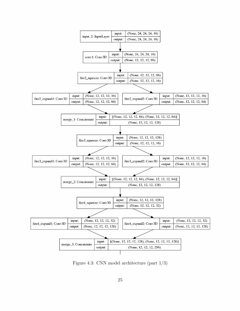
Figure 4.3: CNN model architecture (part 1/3)

25

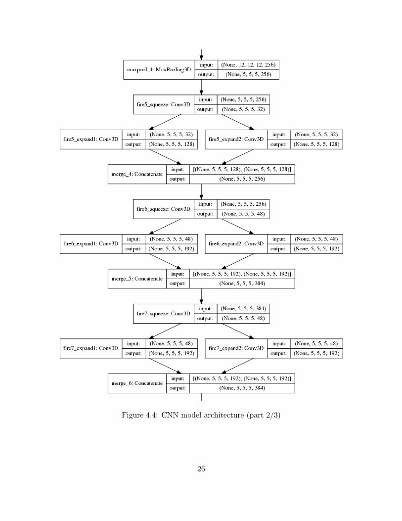
Figure 4.4: CNN model architecture (part 2/3)

26

Figure 4.5: CNN model architecture (part 3/3)

Each of these building blocks has a “squeeze” layer that consists of a convolutional layer,

an expansion layer consisting of two convolutional layers and a concatenation layer that

merges the expansion layers back together. There is a max pooling layer followed by the

third building block and an average-pooling layer followed by the last building block. The

output layer is the only dense layer of the model. The total number of learnable parameters

of the model add up to 1,340,769. Adam optimizer was used for optimizing the model and

Glorot uniform weight initialization method was used to initialize the layers.

Implementation

The model was implemented using Keras [1]. The ODDT toolkit [42] and rdkit [2] were

used to read the PDBbind files and molecular manipulations. Training and testing were

27

carried out using two machines (chanti00.utep.edu and chanti01.utep.edu). Each of the

machines have two Intel(R) Xeon(R) CPU E5-2680 v4 @ 2.40 GHz processors, 128 GB of

RAM and 8 GeForce GTX 1080Ti GPUs.

4.3 Results and Discussions

The model was trained on 12 datasets in 12 different training sessions. Each training was

carried out for 100 epochs with a learning rate of 10−4. While training, the model weights

were saved only when a better validation performance was achieved. Figure 4.6 and Figure

4.7 shows the training and the validation loss curves for both the nearest neighbor features

and distributed features respectively.

Even though the training was done for 100 epochs on each of the datasets, the model

achieved its best performances on the validation set within first few epochs in most of

the cases. As shown in the Figure 4.6a, the validation performance on the original (with-

out augmentation) nearest neighbor features was saturated during the early stages of the

training and did not show any further improvements. In fact, the validation performance

on the augmented dataset (90◦ rotated) was decreasing with more training (Figure 4.6b).

A similar pattern was observed when the model was trained on the canonically oriented

dataset except for the one which was randomly rotated (Figure 4.6f). For this dataset, it

took a considerable amount of time to have the loss saturated.

For the distributed features, a similar pattern in the loss curves was observed; the

training loss was decreasing but the validation loss was saturated during the early stages

of the training. Moreover, a rough pattern was observed in the validation loss curves.

Choosing a tiny batch size is the reason for having such patterns. The model’s performance

on the training and the test set is documented in Table 4.1.

28

(a) Original (b) Augmented (90-degree rotation)

(c) Augmented (random rotation) (d) Canonically oriented

(e) Canonically oriented and augmented

(90-degree rotation)

(f) Canonically oriented and augmented

(random rotation)

Figure 4.6: Training and validation losses when trained with nearest neighbor features.

29

(a) Original (b) Augmented (90-degree rotation)

(c) Augmented (random rotation) (d) Canonically oriented

(e) Canonically oriented and augmented

(90-degree rotation)

(f) Canonically oriented and augmented

(random rotation)

Figure 4.7: Training and validation losses when trained with distributed features.

According to the results on the test set, it can be claimed that the nearest neighbor

features were better than the distributed features. The values of R2 were better in case of

30

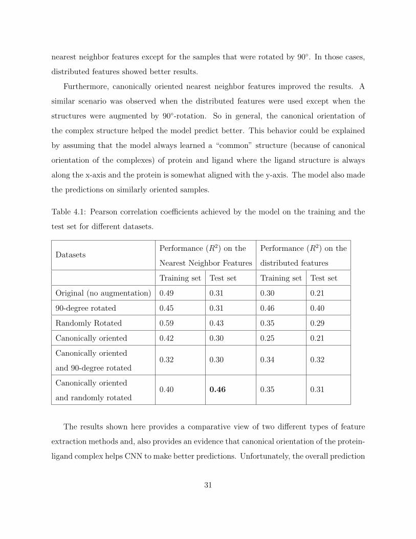
nearest neighbor features except for the samples that were rotated by 90◦. In those cases,

distributed features showed better results.

Furthermore, canonically oriented nearest neighbor features improved the results. A

similar scenario was observed when the distributed features were used except when the

structures were augmented by 90◦-rotation. So in general, the canonical orientation of

the complex structure helped the model predict better. This behavior could be explained

by assuming that the model always learned a “common” structure (because of canonical

orientation of the complexes) of protein and ligand where the ligand structure is always

along the x-axis and the protein is somewhat aligned with the y-axis. The model also made

the predictions on similarly oriented samples.

Table 4.1: Pearson correlation coefficients achieved by the model on the training and the

test set for different datasets.

DatasetsPerformance (R2) on the

Nearest Neighbor Features

Performance (R2) on the

distributed features

Training set Test set Training set Test set

Original (no augmentation) 0.49 0.31 0.30 0.21

90-degree rotated 0.45 0.31 0.46 0.40

Randomly Rotated 0.59 0.43 0.35 0.29

Canonically oriented 0.42 0.30 0.25 0.21

Canonically oriented

and 90-degree rotated0.32 0.30 0.34 0.32

Canonically oriented

and randomly rotated0.40 0.46 0.35 0.31

The results shown here provides a comparative view of two different types of feature

extraction methods and, also provides an evidence that canonical orientation of the protein-

ligand complex helps CNN to make better predictions. Unfortunately, the overall prediction

31

performance of the model was not satisfactory and there are some strong reasons behind it.

First of all, CNN models are very good at image classification and object detection tasks.

Training a CNN model on images is easier than training it on the voxel descriptors. An

image is a 3D matrix (length, width, number of channels), which becomes 4D for a batch.

On the other side, a voxel descriptor is a 4D object (length, width, height, number of

voxel features) that becomes a 5D matrix for a batch. The extra dimension of the training

samples makes the learning of the model much harder compared to when it learns from

images.

Second, the voxel representations of protein-ligand complexes are usually sparse. For

example, the training samples used for this study were more than 99% sparse, which has

a negative effect on the model’s performance. If most of the neurons of a model are zeros,

then it becomes hard for the model to learn and predict the samples. Sparsity occurs in

the voxel descriptors mainly because of two reasons. First, the protein-ligand complexes

are irregularly shaped. Since the model used here is not a fully convolutional network (a

CNN with only convolutional layers), the input shape needs to be the same. In order to

do that, smaller voxel descriptors were padded with zeros which increased the sparsity.

Second, there is a considerable amount of atoms in each protein-ligand structure that do

not have all the attributes, and that resulted in having a lot of zeros in the inputs.

4.4 Concluding Remarks

Using CNNs as scoring functions to predict protein-ligand binding affinities is still a daunt-

ing task as the network needs to deal with very sparse inputs and added dimensions. Rather

than building a new CNN model, this study compared the performances of the model on

different feature types. It was shown that canonically oriented features help the model

learn better. It was also shown that nearest neighbor features are better than distributed

features. A future work on the network architecture would probably be done to increase

the performance of the model.

32

Chapter 5

DLSCORE – A Scoring Function

Based on Feed-Forward Networks

5.1 Introduction

The previous chapter described an attempt to use a Convolutional Neural Network as a

scoring function to predict protein-ligand binding affinities. Since the performance of the

model was not promising, another study was done to investigate the performance of an

ensemble of feed-forward neural networks as a scoring function. This chapter describes the

method of building such an ensemble of networks, called DLSCORE.

5.2 Materials and Methods

5.2.1 Dataset

This study used the same PDBbind (v. 2016) dataset that was used to train the CNN

model. One of its subsets, the refined set was used due to its high-quality data obtained

after applying different filters regarding its binding features and resolution [35, 27].

5.2.2 Protein-Ligand Preparation

The protein-ligand complexes were downloaded from the PDBbind website and then con-

verted from .pdb to a .pdbqt format, which contains additional properties of the complex,

such as partial charges, and atom types. This conversion was necessary in order to obtain

33

the BINding ANAlyzer (BINANA) features [15] that were used to train DLSCORE.

5.2.3 Intermolecular Features (descriptors)

The BINANA algorithm [15] was implemented in NNScore 2.0 [16] in order to characterize

the binding of ligand-receptor complexes and extract the features. These descriptors are

used as the input in the DLSCORE model. BINANA identifies ligand and protein atoms

within a distance of 2.5 A - 4.0 A between them, as well as electrostatic interactions,

binding pocket flexibility, hydrogen bonds, salt bridges, rotatable bonds, π interactions,

among others [15]. A total of 348 features were considered for each protein-ligand complex.

5.2.4 Model Architecture

For the DLSCORE model, only the fully-connected layers were used to build a set of feed-

forward neural networks. The networks in the model consist of multiple hidden layers with

a different number of neurons. Each hidden layer has a weight matrix (W ) with a dimension

ruled by the input size and the number of neurons in that layer. The size of the output

layer is 1 since DLSCORE predicts a value.

Each protein-ligand complex is represented by a feature vector (f = f1, f2, f3 . . . fn) of

size 348. The input layer takes the feature vector, performs a matrix multiplication with

the weight matrix (W1) and then it propagates the information after applying a non-linear

activation function (Rectified Linear Unit (ReLU) [32] in this case) to it. The next hidden

layer takes these values and performs the same operation before propagating these values to

the next layer. It is worth to mention that the probability of each of the neurons information

to be propagated depends on the dropout probability [38]. Here, the dropout probability

was 20% for the input layer and 50% for the hidden layers. The network architecture can

be expressed mathematically as follows:

34

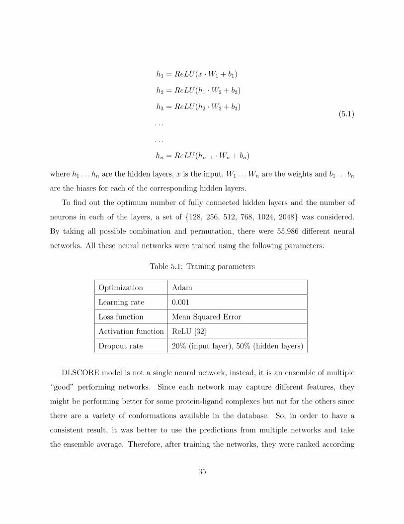
h1 = ReLU(x ·W1 + b1)

h2 = ReLU(h1 ·W2 + b2)

h3 = ReLU(h2 ·W3 + b3)

. . .

. . .

hn = ReLU(hn−1 ·Wn + bn)

(5.1)

where h1 . . . hn are the hidden layers, x is the input, W1 . . .Wn are the weights and b1 . . . bn

are the biases for each of the corresponding hidden layers.

To find out the optimum number of fully connected hidden layers and the number of

neurons in each of the layers, a set of {128, 256, 512, 768, 1024, 2048} was considered.

By taking all possible combination and permutation, there were 55,986 different neural

networks. All these neural networks were trained using the following parameters:

Table 5.1: Training parameters

Optimization Adam

Learning rate 0.001

Loss function Mean Squared Error

Activation function ReLU [32]

Dropout rate 20% (input layer), 50% (hidden layers)

DLSCORE model is not a single neural network, instead, it is an ensemble of multiple

“good” performing networks. Since each network may capture different features, they

might be performing better for some protein-ligand complexes but not for the others since

there are a variety of conformations available in the database. So, in order to have a

consistent result, it was better to use the predictions from multiple networks and take

the ensemble average. Therefore, after training the networks, they were ranked according

35

to their performances on the validation set (see section 5.4) and only the top performing

networks were chosen for the ensemble.

5.3 Evaluation metrics

The networks were evaluated using statistical metrics, including, mean square error (MSE),

mean absolute error (MAE), root mean squared error (RMSE), Pearson (R), Spearman rho

(ρ) and Kendall Tau (τ) correlation coefficients. The mathematical formulae for the metrics

are given below:

MSE =1

n

n∑j=1

(yi − yi)2 (5.2)

MAE =1

n

n∑j=1

|yj − yj| (5.3)

RMSE =

√√√√ 1

n

n∑j=1

(yj − yj)2 (5.4)

R =

∑nj=1(xj − x)(yj − y)√∑n

j=1(xj − x)2√∑n

j=1(yj − y)2(5.5)

where yj and yj represent the experimental and the predicted binding affinity, respectively.

ρ = 1− 6∑d2i

n(n2 − 1)(5.6)

where di is the rank difference for the i-th sample and n is the sample size.

τ =C −DC +D

(5.7)

where C is the number of concordant points and D is the number of discordant points.

The MAE measures the average magnitude of the errors in their binding affinity pre-

dictions, while the RMSE measures the ability of DLSCORE to properly identify a small

prediction range of the predicted vs the experimental values. A confidence limit of 1-2

kcal/mol was chosen to test the scoring functions overall performance.

36

5.4 Results and Discussions

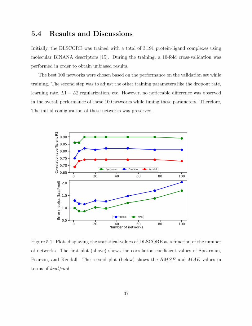
Initially, the DLSCORE was trained with a total of 3,191 protein-ligand complexes using

molecular BINANA descriptors [15]. During the training, a 10-fold cross-validation was

performed in order to obtain unbiased results.

The best 100 networks were chosen based on the performance on the validation set while

training. The second step was to adjust the other training parameters like the dropout rate,

learning rate, L1− L2 regularization, etc. However, no noticeable difference was observed

in the overall performance of these 100 networks while tuning these parameters. Therefore,

The initial configuration of these networks was preserved.

0 20 40 60 80 1000.65

0.70

0.75

0.80

0.85

0.90

Correlation coefficient R2

Spearman Pearson Kendall

0 20 40 60 80 1000.5

1.0

1.5

2.0

Error metrics (kcal/mol)

RMSE MAE

Number of networks

Figure 5.1: Plots displaying the statistical values of DLSCORE as a function of the number

of networks. The first plot (above) shows the correlation coefficient values of Spearman,

Pearson, and Kendall. The second plot (below) shows the RMSE and MAE values in

terms of kcal/mol

37

Since getting a prediction from an ensemble of 100 networks is time-consuming, ensem-

bles of different sizes were analyzed to come up with a smaller ensemble that would show an

optimum performance. The comparative statistics (Pearson, Spearman, Kendall, RMSE,

and MAE) for different size of ensembles (Fig. 5.1) was done and it was noticed that the

optimal performance (highest correlation coefficients and lowest RMSE and MAE) is pos-

sible with the top 10 networks. Moreover, choosing this subset of networks over a hundred

resulted in 10x speedup of the program. Based on the Pearson correlation coefficient, the

default number of networks for the model was chosen to be 10.

When the test set was evaluated using DLSCORE, NNScore 2.0, and Vina, it was

observed that DLSCORE outperformed NNScore 2.0 and Vina (Table 5.2, Fig. 5.2).

Table 5.2: Main statistics of binding affinity predictions of DLSCORE, NNScore 2.0 and

Vina after testing it with 300 refined protein-ligand complexes.

Statistical value DLSCORE NNScore 2.0 Vina

N (sample size) 300 300 300

RMSE (kcal/mol) 1.15 2.78 3.17

MAE (kcal/mol) 0.86 2.03 2.50

Max possible correlation 0.98 0.98 0.98

Pearson Correlation Coefficient 0.82 0.21 0.15

Spearman rho 0.90 0.47 0.39

Kendall tau 0.74 0.33 0.27

When compared the three scoring functions (DLSCORE, NNScore 2.0, and Vina) with

PDBbind (v.2016) refined set, DLSCORE had the optimal performance, getting the closest

values to the experimental data (Fig. 5.3a) in terms of ∆G (The change in free energy

in a chemical reaction) values. Vina obtained 88 protein-ligand complexes (29.33% of the

total data) with a difference less than 1 kcal/mol of the experimental values, 52 data

points (17.33%) within 1-2 kcal/mol boundaries, and 160 (53.34%) were greater than 2

38

12 11 10 9 8 7 6

Experimental G (kcal/mol)

12

11

10

9

8

7

6Pre

dic

ted

G (

kcal/m

ol)

N = 300

<1 1-2 >2

G Error (kcal/mol)

0.0

0.1

0.2

0.3

0.4

0.5

Norm

alized C

ount

(a) Vina

12 11 10 9 8 7 6

Experimental G (kcal/mol)

12

11

10

9

8

7

6

Pre

dic

ted

G (

kcal/m

ol)

N = 300

<1 1-2 >2

G Error (kcal/mol)

0.00

0.05

0.10

0.15

0.20

0.25

0.30

0.35

0.40

Norm

alized C

ount

(b) NNScore 2.0

12 11 10 9 8 7 6

Experimental G (kcal/mol)

12

11

10

9

8

7

6

Pre

dic

ted

G (

kcal/m

ol)

N = 300

<1 1-2 >2

G Error (kcal/mol)

0.0

0.1

0.2

0.3

0.4

0.5

0.6

0.7

Norm

alized C

ount

(c) DLSCORE

Figure 5.2: Graphs showing the predicted values within 1 kcal/mol (dotted line) and 2

kcal/mol (solid line) range. Green dots represent a predicted score less than 1 kcal/mol

away from the experimental value. Yellow dots represent a predicted score between 1

kcal/mol and 2 kcal/mol of the experimental value. Red dots represent a predicted score

greater than 2 kcal/mol away from the experimental value.

39

0 2 4 6 8

0.0

0.2

0.4

0.6

Absolute ∆G difference pred−exp (kcal/mol)

De

nsity

DLSCORE

NNScore 2.0

Vina

(a)

DLSCORE NNScore 2.0 Vina

02

46

81

0

Scoring function

Ab

so

lute

∆G

diffe

ren

ce

pre

d−

exp

(kca

l/m

ol)

(b)

Figure 5.3: Graphs showing the absolute difference between the predicted and the ex-

perimental values in terms of ∆G (kcal/mol) given three scoring functions (DLSCORE,

NNScore 2.0 and Vina). Figure 5.3a displays the density plot behavior. Figure 5.3b shows

the skewness, variability and normality in a side by side box-plot representation.

kcal/mol. NNScore 2.0 got 114 values (38%) less than 1 kcal/mol, 71 (23.67%) between 1-

2 kcal/mol and 115 (38.33%) were higher than 2 kcal/mol. On the other hand, DLSCORE

outperformed the other scoring functions, where 203 data points (67.67% of the total data)

were less than 1 kcal/mol away from the experimental values, 71 (23.67%) were within 1-2

kcal/mol, and the 26 (8.66%) remaining were found outside the 2 kcal/mol boundaries.

Moreover, DLSCORE appears to have less variability, but a bigger number of outliers

(Fig 5.3b), while NNScore 2.0 showed a greater standard deviation, but fewer outliers.

Likewise, Vina displays slightly similar variability with NNScore 2.0, but fewer outliers.

Both NNScore 2.0 and Vina have a max value of approximately 10.17 kcal/mol and 10.36

kcal/mol (respectively) between the predicted and experimental values, while DLSCORE

has a max value of 4.43 kcal/mol.

40

5.5 Concluding Remarks

DLSCORE has proven to be a suitable ensemble of neural networks for making better

predictions of binding affinities of crystalized structures, outperforming NNScore 2.0 and

Autodock Vina. Furthermore, DLSCORE has proven to show more consistency in its

results. The key reason behind its success is using an ensemble of neural networks where the

network architectures are different from each other, enabling those to learn the randomness

of the atomic properties in the molecular structure. Taking an average of the outputs

from 10 different neural networks helped DLSCORE to provide an output that is similar

to the experimental value. So, DLSCORE is a simple (less complicated neural network

architecture) yet more accurate scoring function compared to other popular ones.

41

Chapter 6

Conclusions and Future Work

6.1 Concluding Remarks

This thesis work described the methods of using Convolutional Neural Networks (CNNs)

and feed-forward neural networks in order to build scoring functions for predicting protein-

ligand binding affinities. A comparative result was shown for the CNN model that was

trained with different types of features. It was observed that the nearest neighbor features

were better than the distributed features when they were used to train a CNN model. The

results were further improved by reorienting the molecular structures using a canonical

transformation.

The ensemble of neural networks, DLSCORE, performed reasonably well in predicting

binding affinities. In fact, it outperformed two popular scoring functions NNScore 2.0

and Vina. This study concludes that feed-forward networks are capable enough to predict

binding affinities when used an ensemble of those are used.

6.2 Future Work

In future, following experiments can be carried out for further improvement of the scoring

functions.

• The CNN model used in this study was borrowed from Gomes et al. [18]. But the

feature extraction methods were different than theirs. It would be interesting to see

if a CNN model with a completely different network architecture trained on these

features could make better predictions.

42

• In order to improve the performance of DLSCORE, the ensemble needs to be more

diverse in identifying the molecular structures. The rank-score characteristic function

[20] can be used to select more diverse networks for the ensemble.

• PDBbind refined set was used to train and test the models. There is another dataset,

called DUD-E (http://dude.docking.org/) which is very large and diverse. It would

be interesting to see if the models can make better predictions when trained with a

subset of the DUD-E dataset.

A scoring function is a small part of the virtual screening process in drug discovery.

Those can be used for de novo (starting from the scratch) design of drug molecules as well.

The scoring functions developed in this work will be used to produce novel drug compounds

in the future.

43

References

[1] Keras: The python deep learning library. https://keras.io/. Accessed: 2018-07-31.

[2] Rdkit: Open-source cheminformatics software. https://www.rdkit.org/. Accessed:

2018-07-31.

[3] Ain, Q. U., Aleksandrova, A., Roessler, F. D., and Ballester, P. J. (2015). Machine-

learning scoring functions to improve structure-based binding affinity prediction and

virtual screening. Wiley Interdiscip Rev Comput Mol Sci, 5(6):405–424.

[4] Alberts, B., Johnson, A., Lewis, J., Raff, M., Roberts, K., and Wal-

ter, P. (2002). Molecular Biology of the Cell. Garland Science,

https://www.ncbi.nlm.nih.gov/books/NBK26911/, 4 edition.

[5] Alipanahi, B., Delong, A., Weirauch, M. T., and Frey, B. J. (2015). Predicting the

sequence specificities of dna- and rna-binding proteins by deep learning. Nature Biotech-

nology, 33:831 EP –.

[6] Artemenko, N. (2008). Distance dependent scoring function for describing proteinligand

intermolecular interactions. Journal of Chemical Information and Modeling, 48(3):569–

574. PMID: 18290639.

[7] Ballester, P. J. (2012). Machine learning scoring functions based on random forest and

support vector regression. In Shibuya, T., Kashima, H., Sese, J., and Ahmad, S., editors,

Pattern Recognition in Bioinformatics, pages 14–25, Berlin, Heidelberg. Springer Berlin

Heidelberg.

[8] Ballester, P. J. and Mitchell, J. B. O. (2010). A machine learning approach to predicting

protein-ligand binding affinity with applications to molecular docking. Bioinformatics

(Oxford, England), 26(9):1169–1175.

44

[9] Ballester, P. J., Schreyer, A., and Blundell, T. L. (2014). Does a more precise chemical

description of proteinligand complexes lead to more accurate prediction of binding affin-

ity? Journal of Chemical Information and Modeling, 54(3):944–955. PMID: 24528282.

[10] Bohm, H.-J. (1998). Prediction of binding constants of protein ligands: A fast method

for the prioritization of hits obtained from de novo design or 3d database search programs.

Journal of Computer-Aided Molecular Design, 12(4):309–309.

[11] Chen, H., Engkvist, O., Wang, Y., Olivecrona, M., and Blaschke, T. (2018). The rise

of deep learning in drug discovery. Drug Discovery Today.

[12] Cheng, T., Li, X., Li, Y., Liu, Z., and Wang, R. (2009). Comparative assessment of

scoring functions on a diverse test set. Journal of Chemical Information and Modeling,

49(4):1079–1093. PMID: 19358517.

[13] Cherkasov, A., Muratov, E. N., Fourches, D., Varnek, A., Baskin, I. I., Cronin, M.,

Dearden, J., Gramatica, P., Martin, Y. C., Todeschini, R., Consonni, V., Kuz’min, V. E.,

Cramer, R., Benigni, R., Yang, C., Rathman, J., Terfloth, L., Gasteiger, J., Richard, A.,

and Tropsha, A. (2014). Qsar modeling: Where have you been? where are you going to?

J Med Chem, 57(12):4977–5010. 24351051[pmid].

[14] Deng, W., Breneman, C., and Embrechts, M. J. (2004). Predicting protein-ligand bind-

ing affinities using novel geometrical descriptors and machine-learning methods. Journal

of Chemical Information and Computer Sciences, 44(2):699–703. PMID: 15032552.

[15] Durrant, J. D. and McCammon, J. A. (2011a). BINANA: a novel algorithm for ligand-

binding characterization. J Mol Graph Model, 29(6):888–893.

[16] Durrant, J. D. and McCammon, J. A. (2011b). NNScore 2.0: A Neural-Network

Receptor-Ligand Scoring Function. Journal of Chemical Information and Modeling,

51(11):2897–2903.

45

[17] Duvenaud, D. K., Maclaurin, D., Aguilera-Iparraguirre, J., Gomez-Bombarelli, R.,

Hirzel, T., Aspuru-Guzik, A., and Adams, R. P. (2015). Convolutional networks on

graphs for learning molecular fingerprints. In NIPS.

[18] Gomes, J., Ramsundar, B., N Feinberg, E., and Pande, V. S. (2017). Atomic Convo-

lutional Networks for Predicting Protein-Ligand Binding Affinity.

[19] Hsin, K.-Y., Ghosh, S., and Kitano, H. (2014). Combining machine learning systems

and multiple docking simulation packages to improve docking prediction reliability for

network pharmacology. PLOS ONE, 8(12):1–9.

[20] Hsu, D. F., Kristal, B. S., and Schweikert, C. (2010). Rank-score characteristics (rsc)

function and cognitive diversity. In Yao, Y., Sun, R., Poggio, T., Liu, J., Zhong, N., and

Huang, J., editors, Brain Informatics, pages 42–54, Berlin, Heidelberg. Springer Berlin

Heidelberg.

[21] Hughes, T. B., Miller, G. P., and Swamidass, S. J. (2015). Modeling epoxidation of

drug-like molecules with a deep machine learning network. ACS Cent Sci, 1(4):168–180.

27162970[pmid].

[22] Iandola, F. N., Moskewicz, M. W., Ashraf, K., Han, S., Dally, W. J., and Keutzer, K.

(2016). Squeezenet: Alexnet-level accuracy with 50x fewer parameters and <1mb model

size. CoRR, abs/1602.07360.

[23] Jain, A. N. (2006). Scoring functions for protein-ligand docking. Current Protein

Peptide Science, 7(5):407–420.

[24] Jimenez, J., Doerr, S., Martınez-Rosell, G., Rose, A. S., and De Fabritiis, G. (2017).

Deepsite: protein-binding site predictor using 3d-convolutional neural networks. Bioin-

formatics, 33(19):3036–3042.

46

[25] Jimenez, J., Skalic, M., Martınez-Rosell, G., and De Fabritiis, G. (2018). KDEEP: Pro-

teinLigand Absolute Binding Affinity Prediction via 3D-Convolutional Neural Networks.

Journal of Chemical Information and Modeling, 58(2):287–296.

[26] Joseph-McCarthy, D., Baber, J., Feyfant, E., Thompson, D., and Humblet, C. (2007).

Lead optimization via high-throughput molecular docking. 10:264–74.

[27] Khamis, M. A. and Gomaa, W. (2015). Comparative assessment of machine-learning

scoring functions on PDBbind 2013. Engineering Applications of Artificial Intelligence,

45:136–151.

[28] Krizhevsky, A., Sutskever, I., and Hinton, G. E. (2012). Imagenet classification with

deep convolutional neural networks. In Proceedings of the 25th International Conference

on Neural Information Processing Systems - Volume 1, NIPS’12, pages 1097–1105, USA.

Curran Associates Inc.

[29] Lengauer, T. and Rarey, M. (1996). Computational methods for biomolecular docking.

Current Opinion in Structural Biology, 6(3):402 – 406.

[30] Li, G.-B., Yang, L.-L., Wang, W.-J., Li, L.-L., and Yang, S.-Y. (2013). Id-score: A

new empirical scoring function based on a comprehensive set of descriptors related to

proteinligand interactions. Journal of Chemical Information and Modeling, 53(3):592–

600. PMID: 23394072.

[31] Liu, Q., Kwoh, C. K., and Li, J. (2013). Binding affinity prediction for proteinli-

gand complexes based on contacts and b factor. Journal of Chemical Information and

Modeling, 53(11):3076–3085.

[32] Nair, V. and Hinton, G. E. (2010). Rectified linear units improve restricted boltzmann

machines.

[33] Park, Y. and Kellis, M. (2015). Deep learning for regulatory genomics. Nature Biotech-

nology, 33:825 EP –.

47

[34] Pereira, J. C., Caffarena, E. R., and dos Santos, C. N. (2016). Boosting Docking-Based

Virtual Screening with Deep Learning. Journal of Chemical Information and Modeling,

56(12):2495–2506.

[35] Renxiao, W. (2017). Beginner’s Guide to the PDBbind Database (v.2017).

[36] Rogers, D. and Hahn, M. (2010). Extended-connectivity fingerprints. Journal of

Chemical Information and Modeling, 50(5):742–754. PMID: 20426451.

[37] Shoichet, B. (2004). Virtual screening of chemical libraries. Nature, 432(7019):862–865.

15602552[pmid].

[38] Srivastava, N., Hinton, G., Krizhevsky, A., Sutskever, I., and Salakhutdinov, R. (2014).

Dropout: a simple way to prevent neural networks from overfitting. J. Mach. Learn. Res.,

15(1):1929–1958.

[39] Stefan, R., Fredrik, L., Paul, G., and Svante, W. A PLS kernel algorithm for data

sets with many variables and fewer objects. part 1: Theory and algorithm. Journal of

Chemometrics, 8(2):111–125.

[40] Trott, O. and Olson, A. J. (2010). AutoDock Vina: improving the speed and accuracy

of docking with a new scoring function, efficient optimization, and multithreading. J

Comput Chem, 31(2):455–461.

[41] Wang, R., Fang, X., Lu, Y., and Wang, S. (2004). The pdbbind database: collection of

binding affinities for proteinligand complexes with known three-dimensional structures.

Journal of Medicinal Chemistry, 47(12):2977–2980. PMID: 15163179.

[42] Wojcikowski, M., Zielenkiewicz, P., and Siedlecki, P. (2015). Open drug discovery

toolkit (oddt): a new open-source player in the drug discovery field. Journal of Chem-

informatics, 7(1):26.

48

[43] Zhang, S., Golbraikh, A., and Tropsha, A. (2006). Development of quantitative struc-

turebinding affinity relationship models based on novel geometrical chemical descriptors

of the proteinligand interfaces. Journal of Medicinal Chemistry, 49(9):2713–2724. PMID:

16640331.

[44] Zilian, D. and Sotriffer, C. A. (2013). Sfcscorerf: A random forest-based scoring

function for improved affinity prediction of proteinligand complexes. Journal of Chemical

Information and Modeling, 53(8):1923–1933. PMID: 23705795.

49

Appendix A

A.1 PDB IDs (PDBBind-2016)

A.1.1 Training and Validation set

4cwo, 2w9h, 2xg9, 2drc, 1hmr, 4gr0, 4qy3, 1oe8, 3f3d, 2vpn, 4q9y, 1zdp, 4u6w,

1tpw, 4djw, 2zz1, 1j17, 4oc2, 1r0p, 3jdw, 3sus, 4o04, 4m3p, 1oxr, 3ime, 4ibf,

1iih, 2q54, 3uxd, 3ljz, 4q09, 1ogz, 1ws4, 1adl, 3fvn, 4agl, 4cst, 3t1a, 2yfe,

4aje, 2iw4, 4z0k, 3nw3, 2qbu, 3n1c, 1w5y, 2r23, 4omc, 1o3l, 1uvt, 3cl0, 1q8u,

4zow, 2bpv, 2i4d, 1bp0, 3ohi, 1bv9, 3sue, 3rlb, 2rkd, 4zx1, 4da5, 3slz, 5upj,

2q2a, 3ujc, 1lbf, 2xef, 2x8z, 2g5u, 2y81, 1add, 3fv3, 2xd9, 2fxs, 4ddh, 4det,

3u90, 3gy3, 1ikt, 3rlr, 2wed, 4ysl, 3m40, 2oi2, 4bqh, 4dff, 1ssq, 2ya8, 2b07,

2izl, 4k6i, 1m7d, 4ck3, 3bug, 2yfa, 4b35, 4muv, 1ydk, 4c52, 3su0, 3u8j, 1hee,

4rd3, 1ctt, 4bt5, 2v8w, 2j79, 1pph, 4rsk, 3nzk, 4abe, 5cas, 3ov1, 1qf0, 3qaa,

1mtr, 1os0, 3ebi, 4cg8, 2aqu, 1nny, 4zba, 3oim, 3fvh, 1yq7, 4qtl, 1g3d, 4a4q,

1g74, 2yay, 3gqz, 4xt2, 2zmm, 2wzf, 3zt3, 3tsk, 2zcr, 5c28, 2vmc, 2cli, 1f4x,

5bv3, 4q3t, 4bf1, 1f73, 2nsj, 1oss, 2jiw, 2wos, 2d3z, 4nj9, 4bkt, 3bpc, 4luz,

4q3u, 3mxd, 3b4p, 2q64, 2uwl, 1hlk, 2vpe, 4k3h, 1sl3, 4b5t, 4o0x, 3g5k, 4bf6,

1kuk, 3ip5, 4ogj, 1v2s, 4rvr, 1mrs, 2rio, 1ydr, 2xyf, 3ddg, 4pf5, 3tfn, 1dy4,

4nze, 1hyo, 3f5j, 4kow, 1koj, 1nhz, 1utl, 3wtl, 3igp, 2qwd, 1v7a, 3exe, 4ryd,

3qfy, 1dud, 3ujd, 1qji, 4g0q, 1egh, 3sio, 4p6w, 3cyz, 3gvb, 2sim, 3h5b, 2wuf,

2wly, 1bcu, 4ury, 3o75, 1xkk, 2w47, 4lps, 1c87, 1bn1, 3rv4, 4rqv, 4tkb, 1met,

5c5t, 3p8p, 2iuz, 4kfq, 3ifl, 4p6c, 1oyt, 4ibg, 3uri, 3t01, 1o5e, 3qgy, 3kgu,

2h21, 3agl, 3n7a, 1qkt, 1o2j, 1azm, 1afk, 1g54, 3nu3, 2yhw, 4mme, 2f94, 3vha,

3tf6, 2pvj, 1fkb, 1n0s, 2vsl, 2ewa, 2bqv, 3drg, 3vvy, 1bhx, 1ezq, 3ucj, 1xd0,

50

3iub, 3g2z, 4m8x, 1bq4, 3t84, 1n1m, 1yvm, 3ccz, 4h81, 2v88, 3s75, 3iss, 4bt4,

3ldq, 3zlr, 3t82, 3ao2, 2hnx, 1ypj, 4gj3, 3qw5, 1qbs, 3ppr, 3v4t, 3g0w, 3old,

4k7o, 1cet, 2oxx, 4nbk, 1bn4, 5d1r, 4abf, 3k5v, 4dy6, 3ccw, 1tkb, 1y3p, 2qwf,

3ai8, 3ckb, 1h22, 2qpu, 2wk6, 3k00, 1bzc, 3pyy, 1oar, 2zkj, 4rdn, 4e7r, 1sdv,

3f78, 3fqe, 1ndw, 1if8, 4ufm, 1usn, 4jyt, 4j48, 1qan, 3tt4, 4nja, 2r2w, 3o8p,

4q7v, 3oil, 4g0y, 3zv7, 3m37, 1sw2, 3zso, 1eb2, 3elc, 1hbv, 1ppk, 3hkt, 1duv,

1t5f, 1a1e, 4rr6, 1hsl, 1v0l, 3hzk, 1d3d, 3ttp, 3kek, 1tcx, 1c5s, 1c4u, 3hkn,

4lvt, 1bxq, 1nc3, 2xdl, 4c1u, 3iph, 4djp, 2bpy, 1nvr, 2cbu, 2zym, 4riu, 3oku,

4np9, 3zhx, 4zb8, 4oc0, 4hwo, 2ceq, 4jne, 3f5k, 1jvu, 1b52, 4fev, 3arp, 2j95,

2iko, 1pkx, 4en4, 3kyq, 4llj, 2csn, 2xii, 3pww, 2vw1, 2e2r, 2pov, 3r7o, 2ihj,

4dmw, 3d9z, 2vwm, 3g1v, 4a6l, 1g36, 3std, 4ksy, 1v2o, 4g0z, 3gy2, 3qwc, 4io7,

4zzy, 1kug, 4xit, 2py4, 4btk, 2p7z, 2gz2, 3b68, 4io6, 4phu, 1w5w, 4ymx, 2vvs,

1olu, 3p9m, 2fgu, 4hw3, 3dcc, 2on6, 4zzz, 1g2k, 5tmn, 4oeu, 2wzm, 1pz5, 2ovv,

4fm8, 2glp, 3t6b, 1i9p, 4euo, 4b74, 3zqe, 3p5o, 4q7s, 3mmf, 1y3v, 2wn9, 3mf5,

2gv7, 3f19, 4wkp, 4k4j, 1sqa, 1jsv, 2pgz, 3gi5, 4ezx, 4o07, 3b25, 4hdf, 3el5,

4w9k, 2qd8, 3rz5, 4g5f, 1ro6, 3ip8, 2j77, 1dhi, 1usi, 4oc5, 4iif, 3b27, 2ri9,

2idw, 4do5, 3gbb, 3ovn, 4e5w, 3s71, 3vf5, 2fle, 2f6t, 4hfp, 4h3j, 3hf8, 3nq9,

2q5k, 4gue, 4w9l, 1bzj, 2xbv, 3i7e, 4qd6, 2xb8, 2i19, 3npc, 1fkw, 4w9d, 1v2k,

4o3c, 1lbk, 1fh7, 5aml, 1ec2, 3ehx, 1bai, 3su1, 3ap4, 4isi, 3tkw, 1k1i, 4g0p,

4q4q, 3fx6, 2r43, 3n9s, 4crf, 4loo, 3ekv, 3nex, 4nxv, 3arx, 2azr, 2hmv, 4aji,

1izh, 1ec0, 1uho, 4cu7, 4cg9, 3zll, 3ouj, 4wa9, 3egt, 2z4o, 4i9h, 2weo, 3d1y,

2ewb, 2d0k, 4b0b, 4tqn, 2gv6, 4kxb, 2rd6, 3d52, 4cwf, 2vh0, 3sur, 1afl, 3hk1,

4eoh, 4m2u, 3m35, 4qsv, 4u73, 2gh9, 4dbm, 1hpx, 3u5j, 4deu, 3fed, 4tkh, 1elc,

1cny, 4h7q, 3m3c, 2cbv, 3g1d, 1gar, 4lch, 3wz7, 1fh9, 3mhi, 2j47, 1rpj, 2rfh,

1ql9, 4lzr, 4np2, 4m0f, 3cs7, 4cj4, 4efk, 4ef6, 4ad2, 1oif, 4m2w, 3aid, 4arw,

2xej, 1tnh, 3mhl, 3f6g, 4uye, 1s39, 1enu, 2dri, 3rf4, 1tjp, 5er2, 3qx5, 4ty6,

4uoh, 4daf, 1zoh, 4bcn, 3su4, 1k21, 1ony, 3l4z, 4a6b, 4hj2, 3a2o, 1b6l, 4z93,

2v57, 1f4f, 1hi4, 1fkh, 1d9i, 4bs0, 1iiq, 3pgl, 4lov, 4bco, 1y0l, 3cct, 1e3g,

51

1k1m, 5byi, 3n7o, 3p8o, 4b73, 4b9k, 1qf2, 4m0r, 4or6, 2xab, 1qxk, 3gs6, 2al5,

4myd, 3si3, 2q63, 3dsz, 4k55, 4abd, 3ozt, 3suw, 5a5q, 1zea, 2yaz, 3st5, 3sug,

1om1, 1grp, 1g3e, 3ijh, 1l83, 4tjz, 3tif, 5cbm, 4ygf, 2zdl, 3mz6, 3g0i, 4pin,

3bgz, 1utj, 2qi1, 3ewc, 1ogg, 3dzt, 3s78, 4gzt, 1lyx, 1hxw, 4bah, 4yes, 4ab9,

3b26, 1xgi, 1yp9, 3su3, 4f9y, 3ikg, 2qnn, 4dhl, 5e2p, 1sdt, 1tmn, 4z84, 4iie,

1ajv, 2ojg, 2hzl, 3ivc, 2pu1, 3r16, 1t32, 4xe1, 3m1k, 1r1j, 3h1x, 4ih6, 4o05,

5amd, 3r1v, 4u69, 2q38, 3pcg, 3bvb, 3jzh, 3umq, 4f6w, 3zq9, 2v2q, 3l4y, 3dk1,

3f6e, 1vso, 4mdn, 3lpk, 3dri, 3s8n, 3hku, 2xj1, 1thz, 1mmq, 3vhd, 4epy, 2p15,

4azg, 1fiv, 3o9a, 4y0a, 3eqr, 3vjc, 2usn, 4zx0, 1uou, 3ed0, 1a69, 1yfz, 3suf,

3be9, 2yk1, 1fzq, 2o4r, 2vot, 1fzj, 3l3l, 3i6o, 2qhz, 2cle, 3su5, 4w9i, 1pxo,

4xtv, 2vvc, 3k02, 3ao4, 1yet, 4dv8, 3dx1, 3rr4, 3ozj, 1fh8, 2ayr, 5aba, 4bc5,

4l19, 4qb3, 2f80, 3v5t, 4io4, 3o4k, 1hi5, 3sr4, 1odi, 4nbl, 1zc9, 1gaf, 3th9,

4ll3, 3ibi, 2ha6, 1xt8, 5fl4, 2brb, 1o2w, 1bwa, 3wz8, 3ao5, 3ekr, 4qxo, 4d4d,

3d78, 2r38, 1o5r, 1bty, 3gi4, 3e3c, 5acy, 3suu, 1igb, 4xip, 3nu5, 1q8t, 3rm9,

4lhv, 4jsa, 5cs3, 1dif, 2qm9, 3ffp, 4ymg, 3s8l, 4dkr, 3zi8, 4abb, 4j47, 4mmm,

2ans, 3bra, 4hla, 3lgs, 2o4l, 4q7w, 3fat, 2uy4, 3d7k, 1g45, 4kiu, 4omk, 2f7o,

3upv, 3s0e, 1i7z, 2zda, 5dgw, 1k9s, 4p3h, 1b8o, 3r24, 5bry, 3fv2, 2aoe, 4tz2,

3djq, 4emf, 1sqo, 4qfn, 1m5w, 3q6w, 4cwt, 4qfl, 2d3u, 966c, 1syi, 4kp8, 1xpz,

5cep, 1w5v, 4zo5, 3c39, 3ryv, 2hkf, 3v2q, 4nh8, 4x5z, 2zfs, 4ovh, 2a8g, 2x00,

4xaq, 4nwc, 4x8v, 1msm, 4keq, 4avh, 3zns, 2fqy, 3kjd, 4omj, 4clj, 4tun, 4abh,

2fxu, 3uu1, 1rp7, 1br6, 4ewn, 4j21, 4b5d, 3juo, 1f0s, 1ajx, 4l4z, 1vzq, 1o2z,

4fp1, 2i80, 5ahw, 2pwc, 4jh0, 1ndy, 4bt3, 1a9m, 2b1g, 3m36, 2e9u, 2reg, 4yo8,

3bfu, 4tln, 4cwp, 2qrl, 3qfd, 1f5k, 3kr4, 2o4j, 1xq0, 1q72, 3ejp, 5efc, 1g7v,

1dar, 1trd, 3dnd, 1xr9, 3d4y, 4y8x, 1n5r, 1ppi, 4gzw, 3vtr, 4mr6, 2pk6, 3ebp,

2fzg, 3sv2, 3fuz, 1ua4, 4djx, 3c2f, 4i3z, 1m0b, 4jkw, 4gr8, 3jvr, 2we3, 2p4j,

3wha, 1w4o, 1bnt, 4ih7, 2zwz, 2wm0, 3nu9, 1lgw, 4jyc, 4ejl, 2pbw, 4alx, 3lp7,

2qci, 2x95, 2xbx, 1dmp, 1dqn, 2wyf, 3qxt, 4f7v, 5cbs, 2xxx, 1ew8, 4unp, 1t7d,

2pyy, 4jz1, 3p3g, 1c1v, 4ymh, 3isj, 5cap, 1w13, 4lzs, 3lpl, 4j45, 4rww, 4ipn,

52

3pe1, 2pu2, 5fl6, 1ppl, 4pop, 1k27, 1mfa, 3gba, 1gjc, 4zvi, 3kmy, 4jfm, 1lpg,

3f1a, 4gid, 1n4k, 1b8y, 3v2p, 1qaw, 4i5c, 3qx9, 1m1b, 4ek9, 3h89, 3mof, 1g2l,

3rz7, 4rd6, 3s43, 4psb, 1aj7, 1gai, 2yi0, 3hww, 4w9o, 4mc6, 2v3d, 1p1o, 4ykj,

3ms9, 3ekt, 3k4d, 3pb7, 4b7p, 1k4g, 3fl5, 2zxd, 1r9l, 2fmb, 2r0z, 2wjg, 4xy8,

3ueu, 4rqk, 4i71, 184l, 2wc4, 3u81, 2qtg, 3dne, 3mi3, 2qdt, 4ts1, 2o4s, 4hws,

3vhk, 2h15, 2bt9, 4ajl, 5dwr, 2zcs, 3tzm, 3twp, 2clh, 3wjw, 2hzy, 1h1s, 4azc,

4iue, 3ffg, 4az6, 2xc4, 2qbp, 1fcz, 4m2r, 1bxr, 1sb1, 4f39, 5am6, 4ca6, 2jkh,

3vw2, 2w8w, 1bdq, 2qbr, 1o5g, 5boj, 1c5p, 4kif, 3mss, 3zyu, 1ogx, 3iww, 4io3,

3kmx, 2vwn, 3oaf, 4iic, 3uug, 3nee, 4qpd, 4elg, 4ks4, 4k3n, 4att, 4ei4, 3ljo,

10gs, 1o0n, 2exm, 1fkf, 4gkm, 3b67, 2zb1, 1gx8, 2v2v, 1sbg, 2web, 3p3r, 2vwc,

5egm, 4ynl, 3wgg, 4ndu, 3bkl, 2hnc, 1pro, 1m2x, 1y6r, 2vuk, 4mo4, 4wiv, 3r4m,

2r1y, 1d7i, 2a4m, 1ocq, 4loh, 3pn1, 2pog, 1d7j, 4yml, 3w9r, 4io5, 2qtn, 3mdz,

2p3i, 4gu6, 4g8v, 1f0u, 3l4x, 5afv, 1avn, 3ts4, 2w4x, 3dx2, 3dp9, 1c5t, 4cs9,

1jgl, 4kzu, 4qge, 3fcq, 4msa, 4aqh, 4c9x, 2uy0, 4dew, 1fki, 2vrj, 1c5x, 4ish,

1x8d, 5tmp, 1nm6, 4ezr, 2jjb, 2xjj, 3r5t, 2p4y, 3s77, 4o0b, 3el9, 4n8q, 3fee,

3oe4, 2j34, 1ik4, 4elh, 4lko, 4q08, 4q7p, 3ppq, 4q1w, 1jao, 1pbq, 2afx, 4yth,

1h2k, 1q1g, 4bup, 4x6n, 2r58, 1qbn, 1td7, 1nfx, 3cyw, 3d7z, 1nvs, 1o2r, 4er1,

2v2c, 4fl2, 2p4s, 3d6p, 1cbx, 2euk, 2w8j, 1g48, 1fpc, 4dkp, 1fkn, 2xm1, 4h42,

4zeb, 3r6u, 3g19, 1rr6, 2y7x, 3sjf, 4hpi, 4xu1, 4e1k, 3mhc, 4fai, 3spf, 4knm,

2pvk, 1h46, 2jh5, 4whs, 3ge7, 3uod, 3hmp, 4m7j, 4dq2, 3cd7, 4eb8, 4x6m, 2zdm,

4qf7, 3b7j, 1ohr, 4aq6, 1sv3, 1xug, 1o2n, 2qd7, 1laf, 2vc9, 1hk4, 1jcx, 3tza,

4hzm, 3qlm, 1uml, 1xh9, 4b6p, 1ws1, 2xmy, 1fcy, 3zdv, 2z94, 1v2n, 4dsy, 4na9,

3alt, 3cda, 1d2e, 3fhb, 4lm2, 1c84, 4lm0, 3i4b, 3b24, 1h6h, 1jaq, 1li2, 2hjb,

3ru1, 3bva, 2xp7, 3lka, 3daz, 2ygf, 3v5p, 4e6d, 2bvd, 1nvq, 4zei, 2ojj, 4mgd,

2fqo, 2p7a, 4lj5, 3iob, 3d4z, 1c5y, 1g7g, 3ebh, 4m14, 3bv9, 2wlz, 2zx8, 3o5x,

3lvw, 1d4i, 3m3z, 1o36, 4ozj, 3t8v, 3rbu, 4nuc, 5cau, 3d50, 3vf7, 4ij1, 3t0x,

3tz0, 2w5g, 2xb7, 1e1x, 2vkm, 1ebw, 2cf8, 1stc, 4n6z, 4cws, 1p1n, 1x38, 456c,

1pfu, 1uv6, 3zsy, 4q0k, 3n35, 2zy1, 2p53, 1kjr, 3rf5, 2p16, 4b2i, 3tfp, 4ruy,

53

2yel, 1bjv, 4fzj, 3nox, 2b7d, 2ax9, 1e5j, 1m2q, 2flr, 4agp, 2i3h, 3b4f, 1kv5,

1g85, 2wca, 3v7x, 1l8g, 3ejq, 4gr3, 3iqu, 1y6q, 3k4q, 4je7, 3tb6, 2jew, 2x0y,

2r75, 4zji, 3f7h, 3hfb, 2x7t, 1bnw, 1f8c, 4cwr, 5efa, 3ikd, 3oy8, 3k8q, 1srg,

1f4g, 1sln, 1nfy, 1ec3, 2r5p, 1nki, 4qfp, 2bfr, 1syh, 4cga, 1w3j, 1v2r, 1lag,

2wer, 1ghy, 3pd9, 1zs0, 1qbt, 4iva, 3h30, 2qbq, 4pnu, 1e6s, 4z2b, 1yds, 1k1n,

1m2p, 3s8o, 4lkq, 4b9z, 4qgd, 2isw, 2bys, 3zcl, 3ps1, 7std, 3ml5, 3fas, 2bvs,

1hvi, 1txr, 1jak, 4j3l, 1owh, 4r4t, 1ghv, 4f3c, 3o99, 4ahs, 3p5l, 4c6u, 2cn0,

4ad6, 1fao, 2wzs, 4kb9, 1flr, 1k6t, 3n86, 3m6r, 3bqc, 4r4i, 4ge1, 5aol, 3bgq,

5am7, 3v78, 2ylc, 1hps, 3sww, 2h3e, 1w9u, 3ove, 4xmb, 3fql, 4ag8, 1w7g, 1v48,

2pcp, 3str, 3gc5, 3d8z, 4cpw, 3p2e, 4k5p, 4ua8, 3gst, 3cyx, 3g30, 4c2v, 3hek,

4oma, 2y5h, 2qe4, 4qpl, 3gr2, 2yxj, 4bcm, 3e6y, 3uxk, 3sut, 3f7i, 2pk5, 2j2u,

3f70, 2jds, 3cj2, 1v2t, 1wvj, 4owv, 1nwl, 2ez7, 1utn, 4aj4, 3l0v, 4d8z, 4a4w,

2cbj, 3own, 2v7a, 4q8y, 1z1h, 2xht, 2evl, 3upk, 2r9w, 4cgi, 5cqu, 4djq, 3b92,

1qhc, 2a14, 4hdb, 1nja, 3hit, 2qg0, 1c5n, 4b3c, 2xj2, 3ckp, 3nes, 5dqe, 4ruz,

4r4c, 3mhw, 4k7n, 1z9y, 2vk2, 3gc4, 5d21, 2cht, 2buv, 4zwz, 3g31, 4fxp, 2hu6,

3veh, 1z6s, 3uw5, 4hym, 2r9x, 3l4w, 1nt1, 1tng, 1kc7, 3ppp, 4jfk, 1np0, 1g53,

1kui, 1aaq, 2pwr, 2q8h, 3lk8, 1tq4, 3nsn, 4efs, 1hsh, 3nu4, 3g0e, 1bzy, 4erf,

1gi4, 4bks, 2e2p, 4kqp, 5bs4, 1c83, 4djy, 2h4k, 5e8f, 3c4h, 2pq9, 3n8k, 2xn5,

1hvl, 4f9w, 1km3, 2zxg, 1bju, 3l3m, 4w52, 4r76, 2zft, 3lzz, 4br3, 2wej, 4fys,

2aog, 3p8z, 4llk, 2xog, 4cig, 3tfu, 3fj7, 3ekx, 1u1b, 2uz9, 2vo4, 4a6s, 4bam,

4lkk, 3s9e, 4r5t, 1h5v, 2fqt, 3wtm, 3acx, 4k0o, 2i0a, 4lbu, 1mq5, 2ra6, 2xn3,

2xxt, 2yi7, 4eu0, 2qrk, 3a1c, 1v1m, 2ypi, 4tu4, 2cgr, 2vxn, 1ado, 4owm, 4ai5,

1q84, 3eax, 4rd0, 1w5x, 3lpp, 2i3i, 3b66, 3s45, 4db7, 3jvs, 2vk6, 2jdm, 2wc3,

2bza, 3tk2, 5aut, 3djp, 2ogy, 3pn4, 3ipq, 3u10, 1bnq, 4itp, 2y7z, 3lxk, 4xmr,

1hp5, 1qin, 4cps, 4des, 2gst, 3qkd, 4oak, 3re4, 2qzr, 5a7b, 3mfw, 1fch, 1tx7,

2zc9, 1nw7, 1gno, 1k1l, 2hb3, 3f8c, 1p19, 4hf4, 4n3l, 2amt, 1o1s, 1v2u, 2ews,

2nnd, 1zp8, 4ayu, 1igj, 3n76, 3rt8, 4eo8, 1pyn, 1hxb, 2r3t, 2wyj, 4b7r, 3fvk,

2bak, 4llp, 4do4, 3n2u, 2z1w, 4f5y, 1mfi, 3ta1, 1moq, 4gqr, 2cf9, 2f7i, 2ole,

54

3ioc, 1d4y, 2whp, 3q6z, 1hih, 3mxe, 1q5k, 1o3j, 2wec, 3q71, 2psu, 4u70, 3uz5,

3nuo, 3fzn, 1fhd, 2hhn, 4w9c, 4ymq, 1bn3, 3fh7, 3oyw, 1wn6, 3sha, 4mmp, 2hl4,

1f8e, 4gg7, 4ibb, 1ax0, 2v2h, 4og4, 4ciw, 3jya, 3c8a, 1j4r, 4uin, 3u9q, 4q19,

2vwo, 1b55, 2qwb, 4eor, 4lm4, 3ta0, 3v2n, 1mes, 2zfp, 1g52, 1lnm, 4rak, 4b6r,

3zdh, 4jxs, 4zbi, 4tte, 4f3k, 1u33, 2vo5, 2xib, 2vfk, 1mu6, 1m48, 1hii, 2uwo,

1ypg, 4wkn, 1ie9, 3dx3, 5bwc, 2fqx, 4agm, 3kdc, 4qem, 3q1x, 3djx, 1jyq, 2xys,

1kav, 5e2o, 3po1, 3uev, 4pmm, 2zx6, 4tkj, 2jfz, 1kv1, 2std, 1q65, 3zyf, 1njc,

3uex, 3rz1, 1jys, 4hwp, 1xka, 3a5y, 4fnn, 4lm3, 3k99, 3su2, 1zhy, 4jyb, 4fht,

5a2i, 4g8m, 3pe2, 1fzm, 3lq2, 1g1d, 3myg, 4loi, 2f81, 4oiv, 2g94, 4arb, 2r5a,

2xde, 1x39, 1xh4, 1pxn, 3le9, 4b7j, 2zz2, 4mnp, 2qtt, 1li6, 1uwt, 4rlt, 3bgb,

1u1w, 4j46, 4o2b, 1j36, 4q99, 4w9j, 1qb1, 3p58, 4ha5, 1ghz, 1zoe, 1a28, 4r5a,

1swg, 1z71, 3iw6, 2j4g, 3g3r, 2h6b, 3b3s, 4ago, 1c5q, 4jx9, 1ols, 4gfo, 4mrz,

1ctu, 4cpr, 2xdk, 2bo4, 4kwo, 3gbe, 3ggu, 1f5l, 1x8r, 4p5z, 3su6, 2p95, 1ndz,

4l6t, 2ydt, 4q81, 1hi3, 4uof, 3hvj, 4ynb, 1g7f, 2dw7, 4iwz, 1yei, 3huc, 4x8u,

4std, 3t70, 3hs4, 4m8h, 1d4k, 2ce9, 2epn, 4nxu, 4f0c, 4rlw, 4kz7, 3i73, 4dst,

3d8w, 2rkf, 3b65, 3g32, 1lvu, 4f1l, 2wnc, 2c1p, 3cf8, 2o4p, 1nf8, 3p8n, 3m8u,

4wko, 1t4v, 4isu, 1gwv, 4b2l, 2r2m, 1lf2, 3cj4, 2wyg, 1rjk, 2wor, 1m0o, 4l4v,

2qi6, 1gnn, 2x97, 2xj7, 1b8n, 1njs, 4knj, 1ta6, 3l59, 3el4, 4cpt, 1a94, 5dq8,

3n3j, 4poh, 3pgu, 1drj, 4kmz, 4i74, 4r59, 2zq2, 2jdu, 3dx4, 3e5a, 3bft, 1xap,

2zjw, 3uo4, 1lkk, 4agq, 3w9k, 3dbu, 3bxg, 1cnw, 1zsf, 3ocp, 1atr, 3hkw, 1c86,

2uy3, 3b7r, 3ng4, 1g32, 2ces, 1u0g, 3ni5, 1aid, 3gy7, 3hll, 2xhm, 2cbz, 3d1x,

1apv, 4gqp, 2cgf, 3x00, 4fk6, 2ihq, 3u6h, 4cd0, 4crl, 1o0h, 2afw, 1bxo, 2a5s,

3p3s, 3hky, 3ok9, 1q54, 4gj2, 3e5u, 4dfg, 3zsq, 1k22, 1w0z, 4uyf, 4gbd, 4ra1,

2xeg, 1b57, 4jal, 4flp, 4de5, 1ele, 2pqz, 1j14, 4xty, 4ly9, 3evd, 5c3p, 2ydw,

2x4z, 1alw, 4rrf, 3wmc, 1c5c, 4gql, 1ps3, 4zl4, 1fq5, 2f8g, 3d83, 4mss, 2pym,

4x50, 2nmx, 3q44, 4s1g, 3utu, 4io2, 2v59, 3gk1, 4knn, 4y79, 2hoc, 3ldp, 4h85,

2wky, 1if7, 2v54, 1ydt, 1pa9, 3b2q, 4i8n, 4qj0, 5c8n, 4qf8, 2wnj, 3p7i, 4l9i,

1yej, 1onz, 1d3p, 2pqb, 3imc, 4z1k, 2xyd, 4nbn, 4bao, 2d1n, 2vb8, 4x5y, 2ypo,

55

4dko, 3qbc, 4i7k, 1o2o, 3vfa, 1s5z, 4q4r, 3wz6, 4cmo, 3rv8, 1ft7, 1vyg, 4etz,

4i7j, 3fv1, 3vje, 4urz, 2cej, 1jq8, 4qp2, 4egk, 4ykk, 4mrg, 3t60, 2gss, 3qqs,

2aoc, 3hmo, 3wzn, 1ciz, 4de0, 2q7q, 2yfx, 1e1v, 2i2c, 2vj8, 1ftm, 2xc0, 2zcq,

3kmc, 1bhf, 1n4h, 4ih3, 2q8z, 3cj5, 2j78, 1g7q, 4fz3, 4nku, 3arq, 3prs, 4n7u,

2rcn, 4ipi, 2jg0, 1gpk, 3rlp, 3td4, 5c1w, 4ahr, 2wvt, 1hmt, 2y80, 3djo, 4xu0,

1nfu, 3b1m, 1fcx, 2b1i, 3uew, 1njd, 4app, 1o3d, 1m7y, 4fsl, 1nc1, 2p3a, 2j7f,

4crb, 4i72, 2o4n, 2fw6, 4k18, 1b38, 2vw5, 4e9u, 2avs, 3aho, 2i4x, 3b7i, 1eoc,

1tni, 4x5q, 4qij, 1bma, 2w08, 3pd8, 3a1e, 3ipu, 3cdb, 2wb5, 4x3k, 5c2a, 3ubd,

2b9a, 1zog, 1j01, 3lzs, 1o0m, 1k6p, 2fpz, 1x8t, 4zec, 3ekw, 3m3x, 3shc, 4ddk,

1efy, 2zn7, 4iuo, 4u43, 4u54, 1c70, 3aaq, 3dhv, 4jss, 3u8k, 3qto, 1jlr, 4u8w,

1rtf, 3oe5, 1dzk, 1xhy, 1zfq, 4zyf, 1o38, 4ezz, 3hb4, 1eld, 4qll, 4pv5, 3lir,

3tay, 4cc5, 4zme, 3cfn, 1jqy, 1hpo, 3pwk, 4exs, 4og3, 4qgi, 2p3b, 3zm9, 1a4k,

3vbd, 1i9n, 4m2v, 3u93, 2vzr, 1o30, 3bl0, 3acl, 1ur9, 3ml2, 1e2l, 2gvv, 1ui0,

3uil, 3d1z, 3rz0, 1i37, 1lpz, 2w67, 2yge, 4poj, 3p9l, 4qrh, 1hvr, 1f8b, 3dgo,

2j75, 3rm4, 4ceb, 1siv, 4ytc, 4rpn, 1ksn, 4jfs, 2uy5, 1os5, 1mq6, 4h75, 2vwl,

4hy1, 4nue, 3n0n, 1yda, 2aac, 4q8x, 4x6o, 1hn4, 3f15, 1bv7, 2doo, 1nl9, 4mc1,

1a4r, 2yix, 3f18, 4nnr, 4ej8, 3pcf, 2qpq, 1n3i, 4y2q, 2ra0, 3nim, 2byr, 1f0t,

1rd4, 2v58, 4av4, 4leq, 3i60, 3n2p, 3qtv, 4csd, 4o9w, 185l, 2jkp, 2qhy, 4e4l,

1ql7, 4riv, 1hdq, 2fvd, 1uwu, 3zbx, 1lan, 5e1s, 4non, 4fs4, 1z9g, 3hkq, 4nh7,

3ip9, 2vnp, 1hos, 2o4z, 4qfo, 1bnu, 2wq5, 4pp5, 3ui7, 3kv2, 3zln, 3rux, 1qb6,

1v11, 3c79, 4ql1, 4b33, 1i5r, 4cfl, 4er2, 1uz1, 4x5p, 3u92, 2j62, 3gi6, 2qi4,

4e0x, 4idn, 4ggz, 4i7m, 2psv, 4czs, 5aoi, 187l, 4kz4, 3exh, 3iw5, 1lpk, 4e6q,

1m0q, 3pcj, 1w3l, 4wn5, 3fuc, 4b34, 1gvw, 1olx, 2oxn, 4z0q, 3kgq, 3g34, 3neo,

1dhj, 3ejr, 4ty7, 3f5l, 4kwg, 1w11, 2oc2, 4d3h, 4ucc, 5caq, 1s89, 5cc2, 3a9i,

4zb6, 1b6j, 4xya, 4g90, 4ara, 4ivb, 3f17, 4o0a, 3iod, 4umc, 2hxm, 5ct2, 4rlu,

1ew9, 3tu7, 4q6e, 1pgp, 1uz8, 4m0y, 2wr8, 4ieh, 4nkt, 3dp4, 2rcb, 4r74, 3fzy,

4km2, 3l4v, 1n51, 2qi5, 1tom, 4ih5, 4gny, 5ceq, 2wl0, 1qy1, 4jpy, 3nht, 3hv8,

1hvs, 4bcp, 4gzx, 4ljh, 1nh0, 1bwb, 4pb2, 1fm9, 4q1x, 3fur, 2qnq, 2o4k, 4oag,

56

4q46, 4c1y, 4qac, 4oks, 3hl7, 3iue, 2ot1, 1lah, 4ban, 5std, 3arw, 4xu3, 3ctt,

3pwm, 3t83, 3d0e, 2vvp, 1o2q, 1drk, 3b50, 3b5r, 4f9u, 3ppm, 3gx0, 2qbs, 3m8t,

3n4b, 4ibd, 1x1z, 4pow, 1f74, 1xws, 3c2o, 4emr, 1ex8, 4ido, 3oy0, 1sqt, 4qjw,

1ydb, 1ndv, 3ryy, 1owe, 4aoi, 3zps, 3rz8, 3r4p, 4heg, 4acc, 4nl1, 1v2l, 4pft,

1lee, 2pwd, 3rsx, 3w07, 2zgx, 1mai, 4a4v, 1iy7, 1zgi, 2nn7, 4q1y, 1lhu, 3ttm,

3d6o, 4u6z, 4r0a, 4z1e, 1w4p, 4n9c, 4jym, 2cet, 2p09, 1ii5, 2v00, 1lke, 4rpo,

1bnn, 1mfd, 4n9a, 1e3v, 4p6x, 3b3w, 4igt, 4tt2, 2jgs, 1v16, 2x2r, 1f0r, 3mho,

4z83, 2j4i, 1r5y, 4pfu, 1jmg, 6std, 3lzu, 4zls, 4cl6, 3o56, 2rke, 4xar, 4aia,

4avs, 4xu2, 3pb9, 4gq4, 3qfz, 3ug2, 3pck, 2hmu, 4xir, 3uyr, 4ibk, 1mue, 4e3g,

3o9i, 2yme, 3nhi, 2xm2, 4n6g, 4fl1, 1bcd, 1nq7, 1gi7, 2rk8, 1lgt, 3lxe, 4g95,

4bi6, 3ozg, 4ibj, 2ccb, 1w3k, 4l50, 3bxf, 4o09, 4a6c, 2a5c, 4qew, 3kqr, 2avq,

3ibn, 4x8o, 8a3h, 4m12, 3c89, 3uxl, 3pbb, 2zq0, 4ly1, 2qnp, 1nhu, 2p7g, 2avm,

2a5b, 1a99, 3ryz, 4uac, 1hwr, 1ec9, 4hdp, 3d0b, 3fvl, 2bz6, 3pcn, 3hcm, 1sld,

4qlk, 1g30, 2pwg, 3o7u, 4v24, 1qk4, 2j94, 5aoj, 3wtj, 3iae, 3gss, 4b3d, 3t1m,

1rbp, 4b1j, 3vh9, 4bcs, 3mhm, 1msn, 1kzn, 3d91, 1wm1, 2vvv, 5a81, 1mrn, 1o3f,

1zpa, 4cwn, 1fv0, 4dsu, 3o9d, 4gih, 4bqg, 4auj, 3liw, 4kwf, 4pp0, 3sw8, 4r73,

3ff3, 2oxy, 2x09, 4i9u, 2j7h, 2fzk, 2xyt, 2o8h, 3ahn, 2xnb, 4cp7, 3c2r, 1sh9,

2i4w, 4aci, 2bet, 1wcq, 3sm2, 3ckz, 1d09, 3sk2, 3gcs, 4b76, 3g2y, 4kp5, 4bb9,

1lkl, 4o61, 1pxp, 2wvz, 3s0b, 4ufh, 4kni, 4re4, 1qy2, 1y3n, 4kcx, 1z6e, 2vyt,

2y82, 1rnm, 2vmd, 3nyx, 4u0w, 3sxf, 2pvu, 1wht, 1oyq, 6cpa, 4cjp, 2xda, 1kel,

2b4l, 1g35, 3p4v, 3po6, 4q6d, 4u1b, 2gzl, 2pvm, 3u8n, 3nik, 4axd, 1j16, 2f9k,

3bu1, 3s76, 1ydd, 3rlq, 2fzc, 4b3b, 1m0n, 3c56, 2xei, 3myq, 3t2w, 2qi0, 4v27,

2j7d, 2nn1, 4j7d, 4km0, 4ko8, 4wk1, 4de2, 5yas, 4ivd, 3ip6, 4pp3, 1qxl, 4m8y,

4z1j, 1pr5, 4gqq, 3w37, 4bck, 4mo8, 2qg2, 4duh, 3nyd, 3ebl, 1a9q, 4qnb, 3p17,

3b3x, 1o5a, 1lyb, 3cd5, 1okl, 2qwc, 4mc2, 4mjp, 1m2r, 3vx3, 2v3u, 4h3g, 2haw,

1g2o, 2aj8, 4crc, 3mi2, 3t3u, 3sfg, 3hig, 3s54, 2baj, 3vhc, 2j27, 3k2f, 1d4h,

3k8c, 1nz7, 4rn4, 2r0h, 1h4w, 4de1, 3gkz, 1elr, 3q2j, 1qft, 4tpw, 2za0, 3pfp,

5alb, 5er1, 3mjl, 4oc1, 2za5, 2brm, 3pwd, 4jzi, 1hvh, 2yb0, 2v77, 4fm7, 4q87,

57

3pce, 3jrx, 1xow, 3usx, 1e2k, 3ekp, 4azi, 4lxd, 4b8y, 2br1, 2pow, 4l51, 3zze,

4ht0, 4m0e, 1ogd, 2cen, 3c88, 1f57, 3qps, 4rhx, 4buq, 2pvl, 2fu8, 3s5y, 1dgm,

188l, 4or4, 2ha3, 3coy, 1b6k, 1rql, 4ax9, 2vhj, 3aas, 3zt2, 5azf, 5cp9, 4sga,

2xye, 4pg9, 4e4n, 4xas, 3zj6, 2zdk, 2zx7, 1w4q, 3gm0, 3hp9, 3zsx, 4qhc, 3gdt,

1xjd, 4qyy, 1mh5, 1n46, 3g35, 3bgs, 3zpu, 2fqw, 1vyf, 2bvr, 1utm, 4bqs, 1nfw,

3ozp, 1d4j, 3hvi, 2nmz, 2fxv, 1d4l, 3bzf, 2y5f, 3bkk, 2erz, 2gyi, 3nuj, 4jsz,

1k4h, 2yek, 1oz0, 3kdb, 1f8d, 1uz4, 4msn, 4ocq, 4ual, 3hl5, 3f16, 5e2r, 1qbv,

1str, 2vvn, 2j7g, 3wtn, 4zwx, 3m5e, 1cgl, 1j37, 3lmk, 2jdp, 3dln, 4o6w, 2qta,

2i4z, 3up2, 2pql, 2c3i, 1k1j, 3gta, 4mc9, 4msc, 1qyg, 4xiq, 4ufl, 4qf9, 1epo,

3pb8, 3dc3, 1ecq, 2vw2, 4wrb, 2uxi, 2ymd, 4g4p, 1loq, 3a6t, 2bes, 4yrd, 2zdn,

1o2h, 1no6, 3gnw, 1f4e, 3u6i, 4afg, 3si4, 4lrr, 2vba, 1ugx, 3d51, 1hpv, 3bxh,

1w9v, 2p3c, 5c2h, 2w66, 4q90, 3gtc, 4p5d, 3dd0, 1gj6, 6upj, 3fjg, 4qev, 2q55,

4djv, 1ejn, 1s19, 4ca8, 3kgt, 2v25, 4rrg, 2clk, 3ddf, 1yqy, 3mam, 2ptz, 2ctc,

3gcu, 4ymb, 3f80, 1e4h, 4ht2, 8cpa, 1x8j, 2qmg, 4q4p, 4rux, 3kwa, 3qt6, 4q83,

1bm7, 1jn4, 4ufk, 3wto, 1szd, 5cjf, 2yki, 1ela, 1g98, 3eko, 2vt3, 1wdn, 3rdo,

4gfm, 3fwv, 3tao, 4nvp, 4cwq, 3iof, 3nq3, 1h2t, 1wc1, 4bj8, 4umb, 3vw1, 4v01,

2c3l, 1o33, 3zk6, 4lk7, 1elb, 4lxz, 3bxe, 4avj, 1o5c, 1gi1, 4y5d, 2d1o, 4rfm,

4b6s, 1bgq, 1rpf, 2q88, 1odj, 2c94, 3mfv, 4abg, 3dd8, 4i54, 2pqc, 3czv, 4llx,

3nkk, 1izi, 4a95, 3ryj, 4rfc, 3nb5, 4gii, 4cjq, 2y8c, 1sr7, 3zi0, 2hs1, 1uwf,

4lhm, 3ozr, 4tim, 2bmk, 4wt2, 3c2u, 2xbw, 3cke, 4i8z, 4lar, 1f3e, 1pot, 4m8e,

1pzp, 3cow, 4yzu, 4zip, 1s38, 4i8w, 3f8f, 1eby, 2nsl, 1oba, 2xpk, 3gsm, 2vh6,

2nta, 5dgu, 4baq, 1o7o, 1ebz, 1qbu, 1i2s, 2qu6, 4ea2, 4loy, 2r3w, 2wbg, 1df8,

1od8, 2boj, 4rwj, 3wvm, 2wf5, 3axz, 1fjs, 1m4h, 3eeb, 4q9o, 4x48, 4zek, 2hb1,

4i8x, 2j7e, 4j44, 1atl, 3u5l, 3gjw, 4ca7, 4o0y, 2vpo, 4b5w, 2oi0, 4i7p, 3tmk,

1yqj, 2jh0, 2qwe, 3vfb, 3ebo, 5cbr, 2qi3, 3znr, 2j7b, 2xxr, 3udh, 3bbb, 1m83,

2pvh, 3i9g, 4kn0, 3lea, 3suv, 4twp, 3a1d, 2y5g, 2uyn, 3qxv, 1u71, 1pme, 1fzk,

4trc, 4j22, 5fl5, 2xdx, 4a7i, 4ngm, 1drv, 1zvx, 4b6o, 2bq7, 1lst, 1q91, 4azb,

4kz6, 3t64, 4k0y, 3cd0, 3ehy, 3acw, 4ase, 2tpi, 3kdd, 2qi7, 4f2w, 4d1j, 1a30,

58

3t3c, 4qer, 4kyh, 3bwj, 4djr, 4ayp, 3b3c, 2w8y, 1ivp, 3eb1, 4rj8, 1qk3, 4nyf,

2c92, 4ipj, 4p58, 3ewj, 3c8b, 4qsu

A.1.2 Test Set

3o9p, 1pzi, 3djv, 4pzv, 1pb9, 3mna, 1d4p, 3tvc, 3lp4, 2nt7, 1p57, 3f3c, 2f35,

4hu1, 3buh, 2wkz, 1z4o, 4ngn, 1m7i, 4gu9, 2gl0, 2ves, 3cft, 1det, 3m96, 1swr,

2f7p, 1v0k, 1wur, 1a4w, 4nra, 1d6v, 2r59, 3q7q, 1v1j, 3aau, 4aba, 3uj9, 1c3x,

1mmr, 3i4y, 1fd0, 4x24, 186l, 1gpn, 2rkg, 3ozs, 4kyk, 4j93, 3cm2, 1ype, 2p2a,

4zae, 2bok, 1tsy, 1kyv, 1kpm, 1ppc, 2pyn, 1q8w, 4w97, 2x91, 1vfn, 2jxr, 4fxq,

2uxz, 3s2v, 3jup, 3f48, 4mrw, 1xff, 4ovf, 1hms, 4cp5, 2i6b, 3ryx, 4b32, 4gzp,

1cnx, 4r5b, 4ibe, 1nw4, 2oym, 1qf1, 4fcq, 2vvu, 3lpi, 4zbf, 2bfq, 3iog, 1lzq,

4dkq, 2ya6, 2jh6, 1gvx, 1nli, 2uwd, 4av5, 3kiv, 3o84, 3n9r, 4mhy, 4np3, 1v2w,

4ufj, 1h0a, 3bgc, 1tlp, 1o0f, 3owj, 4hp0, 4g8y, 4cra, 3uw4, 4ad3, 3oyq, 1gfy,

3nx7, 4u0f, 3buf, 3pju, 1usk, 3c52, 2oxd, 4o3f, 3gcp, 1qb9, 1t7j, 1gnm, 4zzd,

3bex, 3f7g, 2f34, 3da9, 1fzo, 3m67, 3h78, 1lrh, 1w96, 3kku, 3t5u, 1k1o, 1xbo,

1nw5, 1lcp, 1ghw, 3ivx, 1qbo, 4lyw, 4ffs, 1c88, 3mzc, 2aod, 4bny, 2bal, 4css,

3eft, 1bnv, 2pou, 1fo0, 4rra, 1g4o, 3roc, 3f8e, 3drf, 3i51, 3bl1, 1h23, 4cjr,

3f68, 3r4n, 1c1r, 4rfd, 4r3w, 2e7f, 4mr3, 4n07, 2f1g, 2i4j, 3p3t, 3rwp, 1g46,

1pb8, 1t31, 1y20, 3k37, 2avo, 1kdk, 1e6q, 4wov, 3s6t, 4aq4, 3jzj, 1v2j, 3v51,

2y7i, 4m6u, 4zzx, 1rmz, 3ag9, 3i5z, 2uwp, 2h6t, 3gy4, 4j7e, 4ovg, 1mjj, 4je8,

4n5d, 1i1e, 3gvu, 4ks1, 3ljg, 3kgp, 3l4u, 1mu8, 3s73, 1fkg, 3brn, 1r1h, 3miy,

4m13, 1q7a, 2x7u, 4del, 3w5n, 1mrw, 3kdm, 3r17, 4ddm, 4pox, 4bi7, 1erb, 2oiq,

4ncn, 2gsu, 1y1z, 3s72, 2uyq, 4ahu, 5dit, 4k77, 4o2p, 4f6u, 3el1, 4bak, 3ies,

4ibi, 4kzq, 2w26, 4dju, 5amg, 1upf, 3f3e, 4c5d, 4der, 3r88, 4oc3, 2cer, 5btx,

2rin, 4y59, 4in9, 4w9p, 4djo, 3qdd, 1mrx, 4hbm, 1hvk, 4ayq, 2ya7, 3gv9, 2h4n,

2h4g, 1pvn, 4mpn, 1sdu, 4kax, 4pcs, 4xxh, 4jia, 4ivc, 2i4u, 1hvj, 4ew3, 3k8o,

2xjx, 4ibc, 2fgv, 1sgu, 3o9e, 1y3x, 2q6f, 4asj, 4pee, 4ehz, 4ou3, 3cz1, 4kz3,

4tmn

59

Curriculum Vitae

Md Mahmudulla Hassan grew up in a small town near Dhaka, the capital of Bangladesh.

He graduated from the University of Dhaka with a Bachelor of Science degree in Physics in

2011. He came to the University of Texas at El Paso in 2014 for pursuing a Masters degree

in Physics. He decided to change his field of study after the graduation and got admitted

to the Computer Science department for pursuing a Master of Science degree leading to the

Ph.D. program. He worked as a Teaching Assistant at the Computer Science department

and as a Research Assistant at the Sirimulla Research Lab in the Department of Pharmacy.

He will be continuing his research as a Ph.D. student of the Vision and Learning Lab and

the Sirimulla Research Lab.

Permanent Address: H#39/D, Mizmizi, Mouchak Road

Shiddhirganj, Narayanganj, Bangladesh

60