deep learning for mind reading: using neural networks to
TRANSCRIPT

Deep Learning for Mind Reading:
Using Neural Networks to Forecast
Neural Signals
Theodor Marcu
Submitted to Princeton University
Department of Computer Science
In Partial Fulfillment of the Requirements for the A.B. Degree
Advisor: Professor Brian W. Kernighan
June 2020

c© Copyright by Theodor Marcu, 2020.
All rights reserved.

Abstract
Brain-computer interfaces have seen unprecedented advances during the past decade.
A particularly interesting area of research is related to speech neuroprostheses: devices
that can translate thoughts directly into speech or text. This work contributes to
the development of speech neuroprostheses by attempting to forecast brain signals
recorded using electrocorticography (ECoG). The applications of this work include
speech forecasting, the modeling of speech producing areas in the brain, and providing
context to models used for brain-to-speech decoding. We use different neural network
models and find that ECoG forecasting is possible with mixed results. While neural
network models can predict a trend associated with the data, modeling the specific
amplitudes proved more difficult. We finish by suggesting a few models that could be
used to improve speech neuroprosthesis research.
iii

Acknowledgements
I would like to express my deep gratitude to Professor Brian W. Kernighan, my
advisor and mentor, for his patient guidance, enthusiastic encouragement, and useful
feedback.
I would like to express my very great appreciation to Professor Uri Hasson and
Professor Karthik Narasimhan for their valuable and constructive suggestions dur-
ing the development of this research work. Their willingness to give their time so
generously has been truly appreciated.
I am particularly grateful for the assistance given by Dr. Ariel Goldstein, Zaid
Zada, Eric Ham, Gina Choe, Catherine Kim, Jimmy Yang, and Bobbi Aubrey, for
their help with preprocessing, analysis, and general guidance with regard to the
project and the data used in it.
I also wish to thank Kate Northrop, my parents, and my family for their unwa-
vering love, support, and encouragement throughout my Princeton undergraduate
experience and beyond.
Finally, I want to thank my friends for the inspiration, energy, and support they
offer me every day.
The author is pleased to acknowledge that the work reported on in this paper
was substantially performed using the Princeton Research Computing resources at
Princeton University which is consortium of groups including the Princeton Institute
for Computational Science and Engineering and the Princeton University Office of
Information Technology’s Research Computing department.
iv

I pledge my honor that this paper represents my own work in accordance with
University regulations.
v

To my family.
vi

Contents
Abstract . . . . . . . . . . . . . . . . . . . . . . . . . . . . . . . . . . . . . iii
Acknowledgements . . . . . . . . . . . . . . . . . . . . . . . . . . . . . . . iv
List of Tables . . . . . . . . . . . . . . . . . . . . . . . . . . . . . . . . . . ix
List of Figures . . . . . . . . . . . . . . . . . . . . . . . . . . . . . . . . . . x
1 Introduction 1
2 Related Work 10
3 Data Collection and Preprocessing 16
3.1 Collection . . . . . . . . . . . . . . . . . . . . . . . . . . . . . . . . . 16
3.2 Preprocessing . . . . . . . . . . . . . . . . . . . . . . . . . . . . . . . 19
3.3 Data Normalization and Binning . . . . . . . . . . . . . . . . . . . . 20
4 Methods and Results 24
4.1 Problem Definition . . . . . . . . . . . . . . . . . . . . . . . . . . . . 24
4.1.1 Time Series Modeling . . . . . . . . . . . . . . . . . . . . . . . 25
4.1.2 Evaluation Metrics . . . . . . . . . . . . . . . . . . . . . . . . 28
4.2 Data Generator . . . . . . . . . . . . . . . . . . . . . . . . . . . . . . 31
4.2.1 Data Batches and Samples . . . . . . . . . . . . . . . . . . . . 32
4.2.2 Data Sampling . . . . . . . . . . . . . . . . . . . . . . . . . . 33
4.3 Models and Experiments . . . . . . . . . . . . . . . . . . . . . . . . . 36
vii

4.3.1 Prediction Task . . . . . . . . . . . . . . . . . . . . . . . . . . 37
4.3.2 Electrode Selection . . . . . . . . . . . . . . . . . . . . . . . . 37
4.3.3 Baseline Approach . . . . . . . . . . . . . . . . . . . . . . . . 38
4.3.4 Linear Regression . . . . . . . . . . . . . . . . . . . . . . . . . 40
4.3.5 Neural Networks . . . . . . . . . . . . . . . . . . . . . . . . . 42
4.3.6 Encoder-Decoder Framework . . . . . . . . . . . . . . . . . . . 49
4.3.7 Temporal Convolutional Network . . . . . . . . . . . . . . . . 51
4.3.8 WaveNet . . . . . . . . . . . . . . . . . . . . . . . . . . . . . . 54
4.4 Complete Results . . . . . . . . . . . . . . . . . . . . . . . . . . . . . 57
4.5 Limitations . . . . . . . . . . . . . . . . . . . . . . . . . . . . . . . . 59
5 Discussion, Future Work, and Conclusion 61
5.1 Discussion and Future Work . . . . . . . . . . . . . . . . . . . . . . . 61
5.2 Conclusion . . . . . . . . . . . . . . . . . . . . . . . . . . . . . . . . . 63
A Code Availability 65
Bibliography 66
viii

List of Tables
4.1 Top 5 Electrodes by MAE (Baseline One-to-One Task). . . . . . . . . 38
4.2 Top 5 Electrodes by MAE (Linear Regression One-to-One Task). . . . 38
4.3 One-to-one Validation and Testing Results . . . . . . . . . . . . . . . 57
4.4 Many-to-one Validation and Testing Results . . . . . . . . . . . . . . 58
ix

List of Figures
1.1 Electrocorticography (ECoG) Diagram . . . . . . . . . . . . . . . . . 3
1.2 Many-to-one electrode prediction example using a simple model. . . . 6
1.3 WaveNet Many-to-one Forecasting (50s). . . . . . . . . . . . . . . . . 9
4.1 Kernel Density Estimate of the Pearson r correlation coefficients for
an LSTM Encoder-Decoder model validation batch. . . . . . . . . . . 30
4.2 LSTM EncoderDecoder Modelgenerated graph of predictions vs. targets. 31
4.3 Window-based sequence prediction diagram. . . . . . . . . . . . . . . 31
4.4 Batch-to-file mapping diagram. . . . . . . . . . . . . . . . . . . . . . 35
4.5 Baseline Prediction Example (6 seconds) . . . . . . . . . . . . . . . . 39
4.6 Baseline Prediction Example (6 seconds, Poor Performance) . . . . . 39
4.7 Baseline Prediction Example (50s Sequence, Validation Set) . . . . . 40
4.8 Baseline Prediction Example (50s Sequence, Test Set) . . . . . . . . . 41
4.9 Linear Regression Prediction Example (50s Sequence, Validation Set) 41
4.10 Linear Regression Prediction Example (50s Sequence, Test Set) . . . 42
4.11 Artificial Neuron . . . . . . . . . . . . . . . . . . . . . . . . . . . . . 43
4.12 Neural Network Architecture with Two Hidden Layers . . . . . . . . 44
4.13 Training vs. Validation Loss for Baseline One-to-one Neural Network
Model . . . . . . . . . . . . . . . . . . . . . . . . . . . . . . . . . . . 46
4.14 Baseline Neural Network Prediction Example (50s Sequence, Valida-
tion Set) . . . . . . . . . . . . . . . . . . . . . . . . . . . . . . . . . . 46
x

4.15 Baseline Neural Network Prediction Example (50s Sequence, Test Set) 47
4.16 Baseline Neural Network Many-to-one Prediction Example (50s Se-
quence, Validation Set) . . . . . . . . . . . . . . . . . . . . . . . . . . 48
4.17 Baseline Neural Network Many-to-one Prediction Example (50s Se-
quence, Test Set) . . . . . . . . . . . . . . . . . . . . . . . . . . . . . 48
4.18 LSTM Encoder-Decoder Neural Network One-to-one Prediction Ex-
ample (50s Sequence, Validation Set) . . . . . . . . . . . . . . . . . . 50
4.19 LSTM Encoder-Decoder Neural Network One-to-one Prediction Ex-
ample (50s Sequence, Test Set) . . . . . . . . . . . . . . . . . . . . . 50
4.20 TCN Neural Network One-to-one Prediction Example (50s Sequence,
Validation Set) . . . . . . . . . . . . . . . . . . . . . . . . . . . . . . 53
4.21 TCN Neural Network One-to-one Prediction Example (50s Sequence,
Test Set) . . . . . . . . . . . . . . . . . . . . . . . . . . . . . . . . . . 53
4.22 TCN Neural Network Many-to-one Prediction Example (50s Sequence,
Validation Set) . . . . . . . . . . . . . . . . . . . . . . . . . . . . . . 54
4.23 TCN Neural Network Many-to-one Prediction Example (50s Sequence,
Test Set) . . . . . . . . . . . . . . . . . . . . . . . . . . . . . . . . . . 54
4.24 WaveNet One-to-one Prediction Example (50s Sequence, Validation Set) 55
4.25 WaveNet One-to-one Prediction Example (50s Sequence, Test Set) . . 56
4.26 WaveNet Many-to-one Prediction Example (50s Sequence, Validation
Set) . . . . . . . . . . . . . . . . . . . . . . . . . . . . . . . . . . . . 56
4.27 WaveNet Many-to-one Prediction Example (50s Sequence, Test Set) . 57
xi

Chapter 1
Introduction
Brain-computer interfaces (BCI) represent devices or processes that allow the brain
and central nervous system (CNS) to transmit and receive information directly from
an external device [1, 2, 3, 4, 5]. BCIs allow neuroscientists and neuroengineers to
study the human brain and improve the quality of life for people suffering from motor
speech disorders or neurodegenerative diseases [6, 7, 8, 9, 10, 11]. In addition to
health-related applications, BCIs have also been of interest to computer scientists
and researchers interested in artificial intelligence because of their applications in
enhancing human intelligence with the help of computers [12, 13].
BCIs have a wide range of uses today: neuroprosthetic applications, neurofeed-
back, closed- and open-loop brain stimulation, pathophysiology, neuroplasticity, and
neural coding [1]. Neuroprosthetic applications refer to tools and devices that can
augment or enhance the functions performed by the neural system. These range from
devices that are widely-used, like cochlear implants, to applications that are still
undergoing research and development, such as speech prostheses and robotic limbs
[14].
1

Neuroprosthetics and Speech
Research in the past decade has shown incredible advances in neuroprosthetics. The
goal of neuroprosthetics is to bypass intermediaries and directly connect a patient’s
brain to a computer in order to facilitate communication, mobility, and other functions
that might have been lost as a result of disease or illness [15]. For instance, Nuyujukian
et al. created a system that allows paralyzed individuals to control a commercial-grade
tablet and navigate the user interface together with all the available applications
using a Bluetooth-based cursor [16]. The real-time aspect of this task showcases
the incredible advances made in the creation of brain-computer interfaces in the last
decade.
A particularly interesting area of research is related to speech prostheses. Current
state-of-the art devices rely on eye tracking or modified computer peripherals [17].
These technologies provide a low bandwidth medium and might not work for those
suffering from serious cases of total paralysis with loss of speech. For example, most
users of current assistive technologies can barely attain a transmission rate of 10 words
per minute, which is far slower than the average 150 words per minute for natural
speech [17]. Furthermore, typed speech carries a limited emotional and contextual
load when compared to spoken speech, which reduces the subjects’ ability to express
themselves fully. While current technologies allow paralyzed individuals to use a
commercial device in real-time, the bandwidth for such devices is limited to each
individual’s ability to move a cursor on a screen [18]. As many of us are aware, trying
to use a cursor to compose text can be a daunting task. This is because our ability
to think and speak far outpaces our ability to quickly move a pointer on the screen
across a keyboard.
An interesting solution to this problem is creating a speech neuroprosthesis. A
speech neuroprosthesis allows subjects to speak or type with the help of recordings of
brain activity rather than modified computer peripherals [19]. By translating neural
2

signals directly into speech and text, the prosthesis would drastically improve the
communication rate of speech prostheses.
Some of the early work on speech synthesis focused on prediction frequencies
in the human brain associated with the production of vowels, phoneme classifica-
tion using intracortical microelectrode arrays, and decoding vowels and consonants
[20, 21, 22]. More recently, studies have been done on predicting words and sentences
using intracortical brain activity [23, 17, 24, 25]. These studies rely on electrocor-
ticography (ECoG) signals in order to predict speech using techniques from automatic
speech recognition (ASR), neural networks, principal component analysis (PCA), and
encoder-decoder frameworks, among others. For reference, the placement of an ECoG
array is shown in Figure 1.1.
Figure 1.1: Diagram that shows the placement of an electrocorticography (ECoG)sensor array. Not the grid-like pattern of the sensors. Image credits: Blaus (2014)
The Limitations of Current Work
One of the limitations of current work in the area of speech neuroprostheses is related
to the limited datasets used in the studies. Most research relies on restrictive sentence
3

and question-and-answer datasets like the MOCHA-Timit database [27]. For example,
the work done by Angrick et al. relies on 6 participants who read between 244 and
372 words, which represents a limited dataset for analytic and practical purposes.
The paper written by Anumanchipalli et al. relies on 5 participants who read sets of
sentences from the MOCHA-Timit [29] database, scene descriptions, and free-response
interviews. Each participant had about 1000 sentences each. While Anumanchipalli
et al.’s paper uses considerably more data than the work done by Angrick et al., the
fact that it relies mostly on participants reading texts aloud rather than free-form
conversations reduces the real-world applicability of the results.
Another limitation of current work in this area is related to understanding how
speech is modeled and represented in the brain. While performing brain-to-text and
brain-to-speech conversions is now possible thanks to the work of Anumanchipalli
et al., Angrick et al., Makin et al., among others, their approach is closer to building
a classifier than can match brain signals to speech rather than understanding the
mechanisms that lead to the production of speech. One application of neural networks
in cognitive science and neuroscience is comparing the internal representations of
artificial models to those of real brains [30]. Applied to brain-to-speech applications,
leveraging neural network models to understand the representations of speech could
provide insight into the production of speech in the brain, allowing us to build models
that not only use brain signals to classify specific sounds, but can extract complex
sentences and even full thoughts.
Last but not least, word production is heavily reliant on context. More specifically,
a word at time t is going to be produced by a human with knowledge of words (and
thoughts) at times {t−1, t−2, t−3, ...}, but also at times {t+1, t+2, t+3, ...}. Current
work on synthesizing speech or text from ECoG recordings either ignores future time
steps ([25], [28]), or uses target words from the future in order to synthesize speech
([17]). While the former approach does not include context, the latter approach
4

would be unrealistic for a practical brain-machine interface system since it assumes
knowledge of future target words.
Research Goals
Our work aims to improve upon these limitations by attempting to predict the ECoG
signals that are at the source of speech by using considerably more data. To this end,
we use the data from a set of 40 patients whose brain signals were recorded 24 hours
a day for an entire week. Their brain signals were recorded using intracranial ECoG
electrodes with the goal of treating epilepsy [31]. During the observation period each
patient was fitted with 100-200 electrodes on various brain locations. The electrodes
recorded brain signals in Micro-Volts. During the same time period the patients’
speech was also recorded, which provided us with free-form conversations that are
representative of real-world scenarios.
While previous work [28, 17, 25] has focused mostly on brain-to-speech and brain-
to-text synthetization, our work aims to contribute to the effort of creating practical
speech neuroprostheses by predicting the ECoG responsible for speech. The goal of
this method is to address all the limitations outlined above. First, we aim to provide
more context to different models used to extract speech and text from neural activity.
Second, we hope to better understand the mechanisms that lead to speech generation
in the human neural system. Third, we aim to address some of the limitations of
using limited sentence sets by analyzing data from free-flowing speech.
In order to predict brain signals, we leverage both statistical and deep learn-
ing models which are appropriate for time series forecasting. These include Linear
Regression, LSTM (Long Short-Term Memory), and TCN (Temporal Convolutional
Network) models, among others [32, 33]. Furthermore, since we have access to mul-
tiple ECoG electrodes per patient, we attempt both one-to-one and many-to-one
forecasting. One-to-one forecasting refers to using information from one electrode to
5

forecast the series for the same electrode in the future, while many-to-one forecasting
refers to using multiple electrodes to predict the signal of one electrode.
Overview of Results
Our results show that forecasting ECoG signals using different models can be achieved
with varying degrees of success. In both one-to-one and many-to-one scenarios, we
achieve a mean absolute error (MAE) of as low as 0.2 for some electrode samples,
which highlights relatively good prediction rate. Similarly, we can calculate correla-
tion coefficients between −0.9 and 0.9 for pairs of predicted and target time series,
where −1 indicates a perfect negative correlation, 0 indicates no correlation, and 1
indicates a perfect positive correlation. This means that we are able to extract trends
from the data, which can help us address all the limitations mentioned above. One
example is visible in Figure 1.2.
Figure 1.2: Example of an electrode prediction generated by a simple many-to-oneneural network model. The MAE for this specific sample is 0.29, while the correlationis 0.6, which indicates a positive correlation between the target and predicted timeseries.
While specific samples and electrodes show that it is possible to predict some
signals, statistics that look at multiple samples from one batch (between 512 samples
6

and 1024 samples) or full conversations show that the MAE jumps higher while the
correlation is closer to 0. Based on test set performance, the top neural-network
model for both many-to-one and one-to-one prediction is WaveNet, which was initially
developed by Google DeepMind to generate raw audio waveforms [34]. WaveNet
achieves a MAE as low as 0.572 (Correlation Coefficient: 0.504. Closer to −1 or 1 is
better.) on the validation set and 0.744 (Correlation Coefficient: 0.175) on the test set
for one-to-one predictions. For many-to-one forecasting, WaveNet achieves a MAE
of 0.641 for the validation set and 0.747 for the test set, which is similar to results
for one-to-one prediction. Complete results are shown and discussed in Chapter 4
(Section 4.4) and Chapter 5 (Section 5.1).
While WaveNet performed very well compared to other neural-network based mod-
els, one-to-one Linear Regression performed best across the board, achieving a MAE
of 0.469 on the test set with a correlation coefficient of 0.598. We discuss possible
reasons for this in Chapter 5.1.
The overall results of these experiments were mixed, since we did not see the
forecasting ability we were hoping to. While direct speech and text decoding from the
predicted signal is unlikely, the results provide an avenue for future work that will lead
to better speech neuroprosthetics. For example, our work could be used to improve
speech decoding for real-time models described by Anumanchipalli et al., Moses et al.
and Makin et al.. This is because the predicted sequences could be leveraged to
provide context and guide the neural network architectures used to extract speech
brain signals.
Predicting ECoG signals might also be difficult because of the nature of the record-
ings. The electrodes in an ECoG sensor array capture signals from the neurons present
in the specific area where the array was placed, and while the signal-to-noise ratio for
ECoG is better than for other types of sensors, it is still possible that these sensors
may capture noise and/or irrelevant signals [35, 36]. Furthermore, most research on
7
ECoG signal decoding has been done in the context of decoding motor movements
and speech, which highlights the wide range of signals that can be found at that
level [36]. This implies that predicting general signals might be hard, as they encode
multiple different streams of information at once.
Similar to eavesdropping on a wireless or wired signal, eavesdropping on the neural
signal can provide a high signal-to-noise ratio, but it might not provide insight into
the contents of the signal. This is analogous to detecting and attempting to decrypt
data packets by eavesdropping on a Wi-Fi or wired network without the necessary
encryption key [37, 38]. In the case of neural signals, focusing and guiding neural
network models during training with the help of external stimuli like movement fac-
tors, speech, or kinematics can act like a key that enables the models to differentiate
between relevant signals and noise.
In order to solve this problem, a model is described in Section 5.2 that would
leverage speech transcripts during training to guide the neural network model for a
forecasting task. While this information would not be used for the final evaluation,
it could provide a structured way to forecast ECoG signals for speech. A successful
model could also be translated to other type of information, like kinematics and motor
movements.
The shape of the forecasted signal across longer time periods (e.g. 50s) could be
considered evidence for the idea that ECoG time series prediction requires guidance
from other variables. Figure 1.3 shows that while the predicted signal does not easily
capture the amplitudes of the input signal well, it is still able to model the overall
trend. This means that the individual amplitudes might represent different signals
rather than one cohesive signal.
Poor prediction metrics could also be linked to the individual electrodes being
monitored and the respective subject used. While ECoG signals are generally con-
sistent across long periods of time, we know that different electrodes can sometimes
8

Figure 1.3: WaveNet Many-to-one Forecasting. The total duration of the time seriesis 50s and has been produced using a moving window prediction (more details inChapter 4).
.
become unreliable [39]. Furthermore, the fact that the subject suffers from drug-
resistant epilepsy could also imply damage or erratic brain activations in the areas
being monitored, which may reduce the signal-to-noise ratio in the data [35]. The
limitations of the current study are outlined in Section 4.5 and discussed in Section
5.1.
Structure
The following chapters contain an overview of the background behind this problem
and the methods and experiments used in this study. Chapter 2 includes an overview
of past work as it relates to brain-computer interfaces and speech neuroprostheses.
Chapter 3 contains information about the collection and preprocessing of the data
used in the study. Chapter 4 outlines the experiments, methods, and results per-
formed on the data, while Chapter 5 provides an in-depth discussion of the results
and ideas for future work.
9

Chapter 2
Related Work
This chapter surveys past work done in the areas of BCIs, neuroscience, and deep
learning. We put particular emphasis on analyzing work related to alternative com-
munication devices and speech neuroprostheses.
The State of Brain-Computer Interfaces
Brain-computer interfaces have seen unprecedented advancements during the past
decade. For instance, neuroprosthetics are showing signs of leaving the realm of deep
research and development and starting to become more usable and available to those
who need them. For example, Gilja et al. have proven that a prosthesis that was
initially developed for animal model studies could be translated to humans, allowing
them to achieve unprecedented performance with a cursor-control system that re-
lies on intracortical microelectrode arrays placed in the motor cortex [40]. Similarly,
Jarosiewicz et al. brought BCIs closer to mass-adoption by reducing the number of
recalibrations needed to use a cursor-control prosthesis that relies on intracortical
microelectrode arrays [41]. While previously users could not compose long texts be-
cause the neural signal would change, which would require recalibration, Jarosiewicz
10

et al. combined multiple calibration methods to enable a continuous experience that
improved the quality of life of the patients.
Another result that stands out is the development of a robotic arm controlled
by intracortical brain signals that can be used by a subject to lift a glass and drink
water from it [42]. Given the complexity of the fine motor movements associated with
this task, this result is remarkable. Similarly, visual prostheses promise to give the
blind their sight back through devices that connect directly to their visual cortex,
optic nerve, or retina, stimulating them in order to produce shapes and colors with
the help of an external camera [43]. The most advanced prosthesis at this moment
is the Argus II, which can restore sight in patients who suffer from inherited retinal
degenerative disorders that lead to legal blindness [44].
Closed- and open-loop brain stimulation is another form of invasive BCI. Both act
subconsciously and can help patients suffering from brain disorders like Parkinson’s
and epilepsy through electrodes that can deliver electrical stimuli within the brain
[45, 46, 47]. Deep brain stimulation (DBS) is the most common form of closed-loop
brain stimulation and has been shown to be similar to drugs in some cases when
it comes to treating Parkinson’s [46]. There is also evidence that closed-loop brain
stimulation can help patients suffering from depression [48].
The benefits of non-invasive brain-computer interfaces are becoming increasingly
visible as well. For example, neurofeedback is concerned with enabling a subject to
manage, observe, and influence their conscious and subconscious brain state with the
help of auditory, visual, and tactile stimuli that are controlled indirectly by recordings
of their neural activity [49]. Neurofeedback often relies on electroencephalography
(EEG) sensors which are placed around a person’s head, directly on the scalp [8].
This is in contrast with more invasive methods like Deep Brain Stimulation or ECoG.
Neurofeedback can be used to alter or create new habits, help with meditation, and
even help smokers quit [50, 51]. Additionally, neurofeedback has been shown to be
11
useful in the treatment of attention deficit disorders, and a simple online search can
yield links to neurofeedback clinics and treatments [52].
BCIs may also help us better understand neurological disorders so that we can
develop more effective cures. For example, pathophysiology can benefit from BCIs
that can record and observe the interactions between different groups of neurons [1].
This can enable researchers and scientists to better understand the causes behind
different illnesses, paving the road for better therapies and ways to control symp-
toms. Similarly, BCIs can provide insight into neuroplasticity, which is the study of
how synapses, neurons, and representations change over time in response to different
stimuli and events [53]. This has implications in the study of learning, memory, and
the brain’s ability to heal.
The Role of Brain-Computer Interfaces in Communication
Research into augmentative and alternative communication (AAC) devices shows that
there is a clear need for improved speech prostheses. Movement-sensing technologies,
eye tracking, switch scanning, and supplemented speech recognition (SSR) represent
different AAC branches that can help subjects with complex communication needs
[18]. Nonetheless, their bandwidth is limited. For example, eye tracking attains an
accuracy of 63% when used alone, which provides a significant obstacle for communi-
cation to those who need it [18]. When used with secondary technologies like switch
scanning, eye tracking can reach 93% accuracy, but this still implies a reduced speech
rate and increased cognitive load for the user.
While eye tracking works for some users, others need to rely on other technolo-
gies because of their individual circumstances. For example, supplemented speech
recognition (SSR) helps those with severe motor impairments use speech-recognition
systems more easily [18]. According to Koch Fager et al., SSRs combine classical
speech recognition with other inputs in order to increase usability for those who need
12

it. An example is a device that uses a hybrid approach, combining a keyboard with
speech-recognition. The user can type the first letter of the word he wants to say,
say the word, and the choose between the top most likely candidates. While inge-
nious, this user experience is also extremely laborious, which highlights the need for
solutions with less friction [18].
BCIs as alternative communication devices are not a new idea [18, 54, 55]. For
example, Orhan et al. and Peters et al. have developed non-invasive devices that rely
on EEG sensors in order to enable people to type words and sentences. Nevertheless,
while probably faster than eye tracking devices, this method is still not on par with
human speech.
Brain-to-Speech: Extracting Speech from Brain Signal Recordings
One of the most promising research areas for increasing the quality and rate of speech
for users who rely on today’s speech prostheses is translating signals from the brain
into speech directly [19]. This has been shown to be possible using different machine
learning models that can decode brain signal data directly from subjects [17, 24, 28,
15].
The background for using statistical and computational methods for encoding and
decoding brain signals is based on models of speech and sound representation in the
human auditory cortex and the Superior Temporal Gyrus (STG). [58, 59]. These
areas are sensitive to sound and speech in general, and according to Sjerps et al.
they are shown to play a role in the normalization of sounds so that humans can
understand language irrespective of speaker. Furthermore, according to Yi et al.,
the STG has been shown to leverage temporally recurrent connections in order to
gain a coherent perception speech. This aspect motivates the use of recurrent neural
network architectures in this work.
13

Another aspect that motivates the use of neural network architecture for predicting
brain signals is related to the fact that brain signal prediction represents a sequence-
to-sequence task. Sequence-to-sequence tasks are particularly well-suited for neural
network architectures, especially for recursive neural network architectures [60, 61].
Previous work in this area focused on encoding and decoding brain signals into
speech [17, 28, 8, 62]. Some approaches rely on neural networks (Anumanchipalli
et al. [17], Angrick et al. [28]), while other rely on more traditional tools like the
Viterbi algorithm (Moses et al. [24]), the ReFIT Kalman Filter, or a Hidden Markov
Model (HMM) (Pandarinath et al. [62]).
Anumanchipalli et al. have used two bidirectional long short-term memory
(bLSTM) recurrent neural networks to decode articulatory kinematic features and
acoustic features from the brain. This architecture enables the second bLSTM to
learn both the transformation from kinematics to sounds and also correct the articu-
latory estimation errors made by the first neural network. While the results of their
research are very promising, one disadvantage is that the bLSTM leaks information
from the future, which reduces the applicability of the results in practical scenarios.
A particularly interesting example of using deep learning to extract speech from
brain signals is represented in the work done by Makin et al. [25]. Their research
proves that speech can be decoded directly from ECoG data from epilepsy patients.
The authors evaluated their work using the word error rate (WER) metric, which was
as low as 3% (5% is professional-level speech transcription), which indicates another
set of very promising results.
Makin et al. use an encoder-decoder framework with three main layers: a temporal
convolution layer that can learn local regularities in the data across time and down-
samples the input data to 16Hz, an encoder recurrent neural network (RNN) that
provides a high-dimensional encoding of the entire downsampled sequence, and a de-
coder RNN with teacher forcing that is responsible for predicting words [25]. Teacher
14

forcing refers to exposing the model to some part of the predicted data during train-
ing in order to help it understand what regularities to look for. A noteworthy aspect
of their model pipeline is that they force the RNN encoder to predict speech during
training. According to Makin et al., this approach helps guide the neural network
model during training, helping it distinguish the signal from the noise.
Another exciting result comes from Angrick et al. [28]. The authors relied on a
densely connected convolutional neural network and a WaveNet vocoder in order to
transform the recorded neural signals into an audio waveform. A densely connected
convolutional neural network was trained on each participant independently because
the position of the electrodes and underlying brain topologies differ from person to
person. Then, a WaveNet vocoder is used in order to reconstruct the audio waveform
from the spectral features of speech. The paper states that there is no need to train
multiple vocoders since no mapping between individual and spectral features had to
be learned.
These results highlight the exciting state of speech neuroprosthesis research and
motivate further work in this area. Next, we evaluate the role of ECoG data in speech
synthesis research and discuss preprocessing for the purpose of training and validation
using baseline and neural network models similar to the ones described above.
15

Chapter 3
Data Collection and Preprocessing
3.1 Collection
The data used in this thesis was provided by the NYU Medical Epilepsy Unit in
collaboration with the Hasson Lab in the Princeton Neuroscience Institute. The data
consists of electrical activity recorded from the brain and audio recordings of over
40 subjects suffering from epilepsy. The subjects’ brain activity was recorded using
electrocorticography (ECoG) sensors with the goal of identifying brain areas that
might be responsible for epileptic attacks. According to Kuruvilla and Flink, pre- and
post-operative ECoG recordings enable surgeons and doctors to better understand the
location and limits of the epileptogenic areas in the brain, allowing them to reduce
the long-term side-effects of the surgery on the patients [31].
Electrocorticography Signals
This work relies on ECoG data because of its use in the study of electrical activity
that results from brain activation [35]. According to Crone et al., ECoG recordings
have been used to study motor, auditory, visual, and language-related activity in
the brain with promising results. This makes them appropriate for exploring the
16

development of a speech neuroprosthesis. Furthermore, the long-term consistency of
the ECoG signal recordings also makes it viable for this study [39].
Based on the research done by Jeon et al., the signal resulting from ECoG
recordings has been found to be useful for ERD/EDS (Event-related Desynchroniza-
tion/Synchronization), which refers to the change in amplitude of specific cortical µ
and β rhythms during self-paced voluntary activity. Event-related responses have
been found in both low-γ (low-gamma) frequencies (< 60 Hz) and high-γ (high-
gamma) frequencies (between 60 Hz and 200 Hz). γ (gamma) frequencies are a
particular type of neural oscillations (also known as brainwaves), which correspond to
”synchronous activity of neuronal assemblies that are both intrinsically coupled and
coupled by a common input” [64]. More specifically, according to Arnal et al. γ-band
activity is considered to result from the interaction between inhibitory neurons and
pyramidal cells, which is closely aligned with speech-related timescales. Mid-to-high-
γ activity (40 − 200 Hz) is of particular interest because it contains event-related
activity focused on speech production and comprehension [35, 65, 66, 67, 68, 69].
Each patient’s brain activity was recorded using electrodes placed directly on the
surface of the brain for an entire week, twenty-four hours per day for seven days. There
are different types of ECoG electrode arrays that may be used to monitor brain activ-
ity. The data collected for this work comes from subdural electrodes placed directly
underneath the dura mater (the outermost membrane enveloping the brain and the
spinal cord) and right above the arachnoid membrane, which is the outermost of the
meninges responsible for protecting the brain [35, 70]. Compared to other types of
sensors like Electroencephalography (EEG), subdural ECoG has better spatial reso-
lution because it is closer to the source of the signal compared to other sensors, which
are placed further apart from the brain. For example, EEG is usually accomplished
with the help of electrodes placed on the scalp. This means that the signal is blurred
by the skin, skull, and dura mater [35, 71]. According to research cited by Crone
17

et al., the signal-to-noise ratio for ECoG data is better than for EEG because the
impact from scalp muscle activity is reduced. Furthermore, according to the same
research, an advantage of ECoG is provided by the fact that electrodes are closer to
one another compared to EEG, which further increases the spatial resolution.
The ECoG electrodes used in this study consist of conductive metal slides that are
embedded in a sheet made from silicon [35]. In order to be implanted, these electrodes
require a craniotomy, which is the surgical removal of a bone segment from the skull
in order to provide direct access to the brain. This procedure comes with several
risks, including infection and leakage of cerebrospinal fluids, since the electrodes are
connected to outside devices by wires [70].
The ECoG signals were recorded from 100-200 electrodes per patient at a sampling
rate of 512 Hz. Furthermore, high-γ activity has a low voltage, which means that the
data was recorded in Micro-Volts. While other types of sensors like EEG require an
additional electrode for calibration to be placed on the scalp or on the ear, ECoG does
not usually rely on this technique [35]. This is because a reference electrode might
need to be placed in an area with relatively constant activity, which would require
an additional craniotomy. Furthermore, according to Crone et al., techniques like
common average referencing (CAR) are often employed to reduce the bias associated
with any potential noise in the data.
Audio Recordings
Microphones were also placed in the subjects’ rooms for the purpose of studying the
relation between high-γ activity and speech. The microphones recorded the patients
during the same 24/7 period as the electrodes. This aspect of our project goes beyond
what previous research has achieved in this area because of the large data sample.
Furthermore, the patients’ free speech was recorded rather than specific word sets
like MOCHA-Timit [27].
18

3.2 Preprocessing
After collection, the ECoG signals were preprocessed by the Hasson Lab team in
the Princeton Neuroscience Institute [72]. The preprocessing process includes several
steps. First, the data undergoes despiking, which aims to reduce the number of spikes
caused by seizures or other artifacts. While ECoG signals have a higher spatial res-
olution than other types of sensors, it is still possible that there is interference from
muscle-related electrical potentials, vibrations, or pathophysiological factors [35]. For
example, one of the drawbacks of using ECoG data from epilepsy patients is that the
physiology of their brains can be affected by epilepsy or the brain lesions responsible
for epilepsy [35]. This means that some patients might suffer from serious enough
cases that the signals from their brains cannot be used for analysis. According to
Crone et al., it is common that some patients are excluded from some studies be-
cause of the poor data. One of the major drawbacks of our study is that we do not
have information on the position of electrodes or the pathophysiological state of the
patients.
In order to reduce the potential noise associated with the data, we remove data
points that are in the long tail in terms of outsized amplitudes, namely 4 × IQR
(inter-quartile range). This reduces the magnitude of spikes and provides a more
reliable although less complex signal.
After despiking, the data undergoes detrending, which removes a change in the
mean of the data over time, thus removing any remaining distortions. Detrending
relies on common averaging referencing (CAR), a technique that reduces noise in the
data by up to 30%, which yields more discernible neural signals [73, 35]. According
to Ludwig et al., CAR works by ”taking the sample by sample average of all good
recording sites” to create one reference for all sites. This is subsequently subtracted
from each signal. Recording sites (electrodes in our case) are judged to be appropriate
19

when their root-mean squared error (RMSE) is between 0.3 and 2 times the average
RMSE across all other sites.
The next step in the preprocessing of the ECoG signal data is extracting the
70 − 200Hz frequency range from the signal, which previous literature showed to
contain semantic-related data for human speech [65, 66, 67, 68, 69]. This technique
extracts broadband from a time series in a number of distinct sub-bands and then
averages across normalized sub-bands to provide an estimate of broadband shifts in
power.
Last but not least, the ends of the signals are trimmed and aligned with the au-
dio recordings of the patients using cross-correlation. Periods of silence are trimmed
out completely, which means we are left with data files for each conversation. Each
conversation is then smoothed using a Hamming window function [74, 75]. The pro-
cess of trimming the signal introduces artifacts into the waveform, more particularly
the sudden onset and offset of the signal [75]. Thus, the Hamming window function
shrinks the size of the signal at the edges, which reduces the artifacts inherent to
trimming.
3.3 Data Normalization and Binning
Normalization
In order to prepare the preprocessed data for the statistical and neural network mod-
els we used in this work, we first normalized and downsampled it. Because we have
m electrodes per patient that can be considered their own separate time series, we
performed the following steps on each electrode independently. The first step in the
normalization process is calculating the mean and standard deviation of the pre-
processed ECoG amplitudes across the individual training, validation, and test sets
(to ensure no information leakage from the test set to the process of hyper-parameter
20

optimization and training). Then, we subtract the respective mean for each set and di-
vide by the appropriate standard deviation in order to center the data [60, 76, 77, 78].
More precisely, we normalize the preprocessed value v in every ith electrode using:
vk,i =vk,i − µi,s
σi,s
, ∀i ∈ {0,m}, ∀k ∈ {0, n}, ∀s ∈ {train, validation, test} (3.1)
where vi,k is the value of the preprocessed amplitude at each time step, and µi,s
and σi,s are the mean and standard deviation, respectively, of electrode i in set s.
Centering the data achieves a mean of 0 and a standard deviation of 1. While not
typically required, raw or skewed data can prevent model convergence. Normaliza-
tion increases the performance of the back-propagation algorithm inherent to neural
networks, speeding up training and convergence [76].
Binning
After the normalization process, we downsampled the data from 512 Hz to 20 Hz
through binning. Binning refers to averaging every n points in the original signal to
create a new point. In our work, we chose to average 25 points, which is roughly
equivalent to 50 ms of signal. Binning smoothes the signal by reducing the influence
of errors in ECoG array recordings and any outliers that may results from seizures
or artifacts in the signal. Furthermore, signal downsampling has also been employed
in the past in order to improve the performance of neural-network based models like
LSTMs and TCNs, which try to infer a temporal structure from the data [25]. We
perform binning on each electrode i using:
Bj,i =
!t+25t vt,i25
, j ∈ {0, 1, ..., ⌊n/25⌋}, t = j × 25. (3.2)
21

where Bj,i is the resulting binned data point at index j for electrode i. This results
in a downsampled time series of length ⌊n/25⌋.
Splitting into Train, Validation, and Test Sets
Splitting the data into separate sets for training, validation, and testing is a common
procedure in machine learning and data science [60, 76, 79, 78]. The training set is fed
to the models for training, while the validation and test sets are used for evaluating
prediction accuracy with various metrics. Normally, the training and validation sets
are used for hyper-parameter optimization, which is the process of tuning the model
and the data in order to get better results. Because of this recursive process, infor-
mation from the validation set can leak, leading to overfitting and loss of generality
for the model. A model that is not general also loses its usefulness, especially in
more practical applications. As a result of this, test data is reserved for an objective
evaluation at the end, which is performed by the machine learning practitioner in
order to get an objective assessment of how the trained models perform.
Our raw data is separated in different files. A conversation can be spread over one
or more files. Furthermore, each file contains n × m rows and columns, where each
row represents a binned time step and each column represents an electrode. Thus, we
calculated the number of rows per file in order to determine the distribution of our
data across files. Next, we loaded the file paths into a list and shuffled the list. Using
the number of rows per file, we then split the initial list into two: a training list and
validation list that contains 80% of the data and a test list that contains 20% of the
data. This split ratio is common in machine learning, but given the large amount of
data available we could have also reduced the quantity of data in the test set [60, 79].
After this step, we did another 80/20 train/validation split on the first list in order to
generate a training list and a validation list. Shuffling the file list ensures that each
set contains data from multiple conversations, and data from a single conversation
22

can be separated in up to three sets. This increases the representativeness of each
set, allowing us to interpret the results more easily. We note that once the train,
validation, and test sets were generated, the file path lists were saved to separate files
so that we could run different models across the same split.
23

Chapter 4
Methods and Results
This chapter outlines the methods used to explore the hypothesis that ECoG signals
can be forecasted. In order to test this hypothesis we employ the universal machine
learning workflow described by Chollet [60]. Section 4.1 presents a rigorous definition
of our hypothesis and problem, including measures of success. Section 4.2 expands our
approach to using ECoG data to test this hypothesis. Section 4.3 showcases different
models and methods we employed in order to test our hypothesis, while Section 4.4
highlights the most representative results for each method. Last but not least, we
discuss limitations associated with our study in Section 4.5.
4.1 Problem Definition
Time series forecasting is an important problem in machine learning that has appli-
cations in areas beyond neuroscience, such as economics, web traffic prediction, and
speech generation [60, 80, 77, 78]. In our work, we focus on the task of forecasting the
next ℓ steps of an m-dimensional time series Y that results from ECoG monitoring.
In our case, m represents the number of electrodes per patient and can range between
100 and 200.
24

4.1.1 Time Series Modeling
There are multiple ways to approach m-dimensional time series forecasting. The most
common way is handling each individual dimension as a specific task, which results
in m univariate time series of length n that correspond to each of the dimensions.
According to Mariet and Kuznetsov, univariate time series can be modeled easily by
auto-regressive models [81] and neural network models like Recursive Neural Networks
(RNNs) [60, 78]. Nonetheless, multiple time series might also be correlated between
themselves: in our case, it is possible that multiple electrodes may pick different
aspects of the same brain activation in relation to a specific task. Multivariate models
have been developed in order to capture the relationships between multiple time series.
These include Vector Autoregressive (VAR) models as well as neural network models
like RNNs [82, 60].
Both univariate and multivariate time series methods treat a sample at time t as
a singular step, attempting to capture relations between data samples at times t and
t+1. According to Mariet and Kuznetsov, these types of models are referred to as local
models since they capture information about samples that are close in time. Another
interpretation of m-dimensional data is referred to as sequence-to-sequence modeling,
which considers each of of the m univariate time series as a separate sample drawn
from an unknown distribution [80]. Rather than modeling the relationship between
time t and t + 1, the series learns to map time series of length n− ℓ to sequences of
length ℓ. Popular sequence-sequence models include LSTMs, RNNs, WaveNet, and
TCN [33, 32, 80, 60].
We use the notation devised by Mariet and Kuznetsov to formalize local and
sequence-to-sequence modeling in the context of ECoG arrays. 1 In both cases, we
look at a multi-dimensional time series Y m×n (m electrodes recorded for n discrete
1The notation used in this section makes extensive use of the notation presented by Mariet andKuznetsov [80], whose work provides an overview of sequence-to-sequence modeling for time series.
25

time steps). Because the sampling of the electrode recordings is set at 512 Hz, this
means that Y has n512
seconds of signal. We denote the value of all m time series in
Y at time t with Yt(·) and the value of the i-th dimension with Yt(i). Similarly, Y ba (·)
refers to the sequence of time steps between a and b: Ya(·), Ya+1(·), ..., Yb(·).
Local Modeling
In our work, the goal of the predictive model is to infer the amplitude of the ECoG
recordings at times Y n+ℓn+1 (·) where ℓ ≥ 1 using Y at previous times. In the case of
local modeling each time series in m is split into a training set Zi = {Zi,1, Zi,2, ..., Zi,n}
where:
Zi,t = (Y tt−p(i), Y
t+ℓt+1 (i)), (4.1)
where: p ∈ N, ℓ ≥ 1, i ∈ {1, ...,m}, t ∈ {1, ..., n}. (4.2)
In 4.1 p is equal to the lookback for each input, while k is the length of the predicted
sequence. In univariate settings, we attempt to learn a different hypothesis hi for each
Zi. The goal of the model is to learn a hypothesis function hi : Y1×p → Y 1×k from a
hypothesis set H for each electrode in m while achieving a small generalization error
[80]. Again, using the notation used by Mariet and Kuznetsov, we can define this
process rigorously as:
λ(hloc|Y ) =1
m
m"
i=1
ED[L(hi(Ynn−p(i)), Y
n+ℓn+1 (i))|Y ], p ∈ N, ℓ ≥ 1. (4.3)
In 4.3 we define hloc := (h1, ..., hm) and we try to minimze the generalization error
λ over m electrodes, where E is the expected value of L conditioned on Y , our time
series. L is a loss function that we use to evaluate learning success (we discuss loss
26

functions in more depth in Section 4.3) and D represents the distribution of our target
samples Y n+ln+1 given Y [60, 80].
In simpler terms, we attempt to find a collection of hypotheses hloc that can model
each individual time series independently, minimizing the generalization error. To
evaluate our hypotheses, we use a loss function that allows us to measure our success.
Ultimately, this would result in m models, one for each electrode per patient.
Multivariate local learning works similarly. The only difference is that our training
set is Z = {Z1, ..., Zn}, where:
Zt = (Y tt−p(·), Y t+ℓ
t+1 (·)), (4.4)
where: p ∈ N, ℓ ≥ 1, t ∈ {1, n}. (4.5)
In this case, we aim to find a single hypothesis that maps r electrode time series
(2 ≤ r ≤ m) of length p to w electrode time series (2 ≤ w ≤ m) of length ℓ.
Sequence-to-sequence Modeling
Sequence-to-sequence modeling is similar to multivariate local modeling. Instead of
attempting to find one hypothesis Y p×m → Y l×m we attempt to find one that maps
Y (n−ℓ)×m to Y l×m, where n represent all binned time steps in the data. We find h
that achieves the lowest generalization error through:
λ(h|Y ) =1
m
m"
i=1
ED[L(hi(Yn−ℓ0 (i)), Y n+ℓ
n−ℓ (i))|Y ], p ∈ N, ℓ ≥ 1. (4.6)
In this case, the name sequence-to-sequence comes from the fact that all past values
are mapped to future values, not just the ones closest to the prediction, as is the case
with local modeling [80].Local and sequence-to-sequence models are important to our
27

study because they are intrinsically related to the task of time series forecasting.
In our work we use both in order to determine whether ECoG recordings can be
forecasted.
The approach used in this work combines elements from local and sequence-to-
sequence modeling. For example, we use a local approach when training models
for the one-to-one scenario, but we default to a hybrid approach similar to the one
described by Zhu and Laptev and Mariet and Kuznetsov with regard to many-to-one
models. In this approach, we split the sequences across the temporal axis in order to
get inputs of length p that we use to train a single hypothesis to predict one electrode.
4.1.2 Evaluation Metrics
We evaluate our hypothesis that ECoG signals can be forecasted using two primary
metrics. The first one is calculating the mean absolute error (MAE) between the
target signal y and the predicted signal y. The MAE is computed as follows for y and
y of length ℓ:
MAE =
!ni=1 |yi − yi|
n, i ∈ {1, ..., ℓ}. (4.7)
An alternative to MAE is the Root Mean Squared Error (RMSE). Both are used
extensively in time series forecasting [60, 84]. The RMSE is calculated as follows:
RMSE =
#!ni=1(yi − yi)2
n, i ∈ {1, ..., ℓ}. (4.8)
In our study, we chose to use the MAE for both the evaluation metric and the loss
function because it is less sensitive to outliers [84, 85]. Since the ECoG data contains
a lot of outliers, it is possible that it would be harder for the models to learn if we were
28

to use RMSE. However, there are several tradeoffs inherent to using MAE as opposed
to MSE. For instance, according to Chai and Draxler, calculating the gradient of
a MAE score with respect to certain model parameters can be difficult as a result
of MAE’s reliance on the absolute value. RMSE’s ability to capture outliers may
also be an advantage as it might be able to help the model learn specific amplitudes
more easily than the MAE. Nevertheless, since we are not able to exclude outlier
data points easily in our binned data we chose to use MAE as a loss function and
evaluation metric for this study.
Another metric used in this study to evaluate the quality of the predictions is
Pearson’s r Correlation Coefficient [86]. We use Pearson’s r as a measure of linear
association between the target and predicted series. According to Lee Rodgers and
Nicewander, there are multiple ways to conceptualize Pearson’s r. The most relevant
ones to our project are: correlation as a raw function of scores and means, correlation
as a standardizes slope of the regression line, and correlation as the geometric mean
of the two regression slopes [86]. Thus, we use correlation to determine how close
the predicted signal is to the forecasted signal, whether it follows the same trends,
and whether the regression slopes match. Pearson’s r outputs values between −1 and
1, where 0 means that the two series tested are not correlated, −1 means that the
series have a perfect negative correlation, and 1 that the series have a perfect positive
correlation.
We use the SciKit implementation of Pearson’s r [87]. This implementation cal-
culates the correlation coefficient between the predicted time series y and the target
time series y using:
r =
!(y − µy)(y − µy)$!
(y − µy)2!
(y − µy)2(4.9)
29

where µy and µy are the means of y and y, respectively.
In our study we rely on Pearson’s r after training on longer sequences generated
sequentially by our models. This is because we found Pearson’s r to be unstable with
small sample sizes. For instance, Figure 4.1 highlights how Pearson’s r is distributed
around 0 for a batch of shorter sequences, which indicates that most samples don’t
correlate. Meanwhile, the graph generated in Figure 4.2 has correlation 0.484 and
MAE 0.580, despite being generated by the same exact model.
Figure 4.1: Kernel Density Estimate of Pearson’s r correlation coefficients for anLSTM Encoder-Decoder model’s validation batch. Each correlation was computedon the validation target and predicted series of length 20 (binned ECoG signal). Theinput batch to the LSTM model has shape (1024, 100, 1), which corresponds to 1024samples of length 100 (∼ 5, 000 ms) of 1 electrode. The x-axis represents the rangeof the r value between −1 and 1, while the y-axis represents the probability density.
As a result of this trend, we evaluate each model after training by calculating the
MAE and correlation after predicting 50s from random conversations selected from
the validation and test sets, respectively. For one-to-one settings we take a sequence
of length n = 1100 and we predict sequential time series of length ℓ = 20. For each
window of size 20 predicted by the model, we use the previous 100 time steps. At the
end, we discard the initial 100 time steps and calculate the MAE and correlation for
the resulting two sequences of size 1000 (1000 * 50ms = 50,000ms = 5 seconds). The
process is illustrated in Figure 4.3.
30

Figure 4.2: LSTM Encoder-Decoder Model-generated graph of predictions vs. targets.Pearson’s is r = 0.484 and MAE = 0.580. This figure shows the results after predictinga sequence over longer (50s) periods of time. The x-axis represents the binned timesteps and the y-axis represents the amplitude of the preprocessed, normalized, andbinned signal.
Figure 4.3: This diagram shows how sequences of duration 50s are generated. Eachinput has length 100 and each target has length 20. We use the model to predict 20time steps at a time, after which we move the input window forward.
4.2 Data Generator
After preprocessing, normalization, and binning, the next step in the prediction
pipeline is feeding data to the predictive models. The brain signal recordings for
one patient can consume up to 60GB in disk space. As a result, there can be is-
sues related to loading them into the RAM of a regular computer cluster node and
31

how Numpy arrays are stored. This is problematic because neural networks work by
processing batches of samples that update their internal states. To overcome this
obstacle, we designed and implemented a Keras Generator class that yields batches
of data that can fit into memory [60, 88]. The generator enables batch training us-
ing the Keras deep learning library while reducing the number of file open and close
operations.
4.2.1 Data Batches and Samples
Training data is fed to a neural network model for the purpose of learning [60, 78, 77].
The data is fed forward and backward through the neural network in a process called
backpropagation in order to update the internal states and weights and to minimize
the output of the loss function, which is a measure of error between the target y and
predicted values y. Because the backpropagation algorithm relies on a set of highly
parallelizable computations, it is desirable to increase the amount of data fed to the
neural net at once. As a result, we rely on batches, which contain an arbitrary number
of samples.
A sample refers to a row of data and usually contains an input and output, which
is commonly called a target. The model compares the target to the output in order
to calculate the error and evaluate its learning progress with the help of the loss
function. Samples are also called sequences in time series forecasting [80].
A batch consists of several samples. The batch size can have an impact on the
performance of the model during training and evaluation [60, 77, 78]. A larger batch
size is preferable because it speeds up training when high-performance GPUs are
available [60]. In our case, we used batches that contain between 512 and 2048 sam-
ples, which allowed us to use high-end Nvidia Tesla P100 GPU-enabled clusters made
available by the Princeton Research Computing consortium. Section 4.3 includes
more information on the relationship between batches, neural networks, and training.
32

The generator yields batches of sequence data based on the total number of time
steps in the dataset. Thus, a batch always contains an input with the shape:
X = (batch size, ⌊ lookback
sample period⌋, electrode count) (4.10)
and a target with the shape:
y = (batch size, ⌊ target lengthsample period
⌋, target electrode count) (4.11)
The sample has length lookback (referred to as p in Section 4.1), which is the
number of time steps we use in order to make a prediction. Similarly, the target is
characterized by a delay and a target length (referred to as ℓ in Section 4.1). The
delay refers to the number of time steps between the sample and the target data (i.e.
how far in the future are we predicting) while the target length refers to the length
in time steps of the target data. The sample period allows the generator to yield
downsampled data by omitting certain time steps. For example, if sample period = 2,
every other time step in the given data will be omitted, and a second of signal will
contain 512/2 = 256 time steps instead. This is useful for comparing different model
pipelines in order to better understand what accounts for the performance of the
model, similar to the work done by Anumanchipalli et al. and Makin et al..
4.2.2 Data Sampling
The generator needs to extract batches of samples from files. In this regard, the
generator functions similar to a dictionary, mapping batch indices to data samples
and targets. When the generator is initialized, it calculates the total number of
batches using the total sample count and the batch size. The batch size refers to
33

the number of samples in a batch, usually between 512 and 2048. To calculate the
total sample count, the generator needs to iterate over all data files and get the total
number of rows. Since loading each individual file in memory would constitute an
additional overhead, the generator uses the much faster Numpy mmap (memory map)
mode, which allows the generator to load the shape of the array rather than the con-
tents of the entire file [89]. For each file, the generator reads n = file timestep count,
which is the number of rows that correspond to the total number of time steps for a
brain signal recording. We then calculate the file sample count as follows:
file sample count =file timestep count
(lookback + delay + target length)(4.12)
This prevents us from drawing overlapping samples in the dataset, which increases
the entropy of the data, allowing the neural network to minimize overfitting during
learning [60]. file sample count is then used to compute the total sample count,
but it is also added to a Python dictionary object file map that maps files to their
sample counts.
Naive Implementation
A naive implementation would yield batches of data using a global array of indices of
length total sample count for each sample sample indices = [0, 1, 2, ..., total sample count).
For each batch, we would then find samples by generating an interval of indices
batch indices = [batch index × batch size, (batch index + 1) × batch size. Then,
we use the file map we created above in order to fill the batch with samples and
targets. For each index in batch indices we will open the file associated with it in
file map. Unfortunately, while this method is simple and easy-to-understand, it
adds an unacceptable layer of overhead during training because a worst-case scenario
34
is that a file that contains n batches is opened n times for one batch. For a generator
with batch size = 256, lookback = 128, delay = 0, target length = 1, we saw batch
retrieval rates as high as 500 seconds.
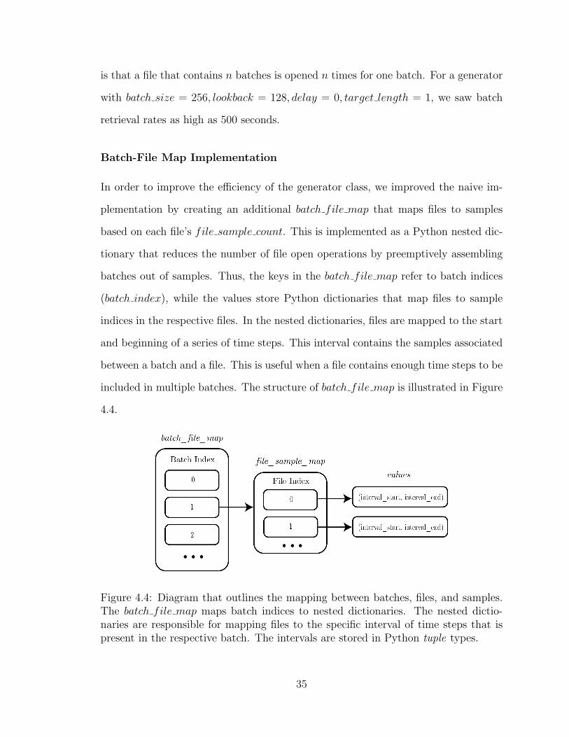
Batch-File Map Implementation
In order to improve the efficiency of the generator class, we improved the naive im-
plementation by creating an additional batch file map that maps files to samples
based on each file’s file sample count. This is implemented as a Python nested dic-
tionary that reduces the number of file open operations by preemptively assembling
batches out of samples. Thus, the keys in the batch file map refer to batch indices
(batch index), while the values store Python dictionaries that map files to sample
indices in the respective files. In the nested dictionaries, files are mapped to the start
and beginning of a series of time steps. This interval contains the samples associated
between a batch and a file. This is useful when a file contains enough time steps to be
included in multiple batches. The structure of batch file map is illustrated in Figure
4.4.
Figure 4.4: Diagram that outlines the mapping between batches, files, and samples.The batch file map maps batch indices to nested dictionaries. The nested dictio-naries are responsible for mapping files to the specific interval of time steps that ispresent in the respective batch. The intervals are stored in Python tuple types.
35

This implementation reduces the number of file open and close operations by
enabling the generator to read all the samples that a file has for a specific batch at
the same time. Generating the map is also not time intensive as we can rely on the
Numpy memory-map mode, which enables quick access to the row count of each file
[89]. While a batch created using the naive implementation might take up to 500
seconds to be generated, a batch created using the batch-file map implementation
can be generated in as little as 1.14 seconds.
4.3 Models and Experiments
We use the binned data in order to determine whether signals recorded from ECoG
arrays during conversations can be forecast. In order to do so, we employ both one-to-
one and many-to-one models. One-to-one models can be considered univariate time
series prediction tasks and can be solved with both local and sequence-to-sequence
modeling techniques. Many-to-one models represent a special case of the multivariate
time series problem described above where we search for a hypothesis function h that
maps Y p×m → Y ℓ×1, where Y ℓ×1 represents the target sequence of length ℓ for one
electrode. Since brain activations are complex in nature and result from interactions
between different areas of the brain, we also hypothesize that using multiple electrodes
to predict the output of one electrode will increase the accuracy of our predictions.
In order to evaluate the task, we leverage multiple types of models and observe the
MAE and Pearson r correlation coefficient on two sequences of length 1000 from the
validation and test set, respectively. The sequences are roughly equal to 50 seconds.
As Section 4.1.2 showed, using longer sequences stabilizes the correlation coefficient
and allows us to determine the performance of a model more reliably.
36
4.3.1 Prediction Task
First, we formalize the parameters of the task. The following models will at-
tempt to forecast the signals from one or multiple electrode samples in batches
of size batch size = 1024 with lookback = 100 bins (equivalent to 5 seconds)
and targetlength = 20 bins (equivalent to 1 second). We only compare results
from binned data, although we note that we have also attempted prediction on
normalized-only data, which is further discussed in Section 4.4. Because the data is
already downsampled through the process of binning, we set sample period = 1.
While some models (e.g. WaveNet) would benefit from a slightly larger batch size
when running on high-performance GPU clusters from a performance standpoint,
modifying the batch size can change the way in which the model learns. As a re-
sult, ensuring that batches have equal size across experiments is crucial to getting
comparable results across the board.
We also note that we only used data from one subject in this study. The subject
was chosen with help from the Hasson Lab team [72]. The subject has a relatively
high signal-to-noise when compared to other subjects, as determined by comparing the
resulting preprocessed data to the raw ECoG recordings. Furthermore, the patient
also has a lot of speech data associated with his ECoG recordings, over 38 hours.
This means that we can use 38 hours worth of speech recordings from the entire 24/7
period (because we trim out the silent periods) in order to test our hypothesis.
4.3.2 Electrode Selection
The subject we analyzed had 114 ECoG electrodes implanted. Because we performed
only one-to-one and many-to-one prediction, we needed to select one electrode we
could compare across data sets. In order to do so, we ran a baseline approach and
a linear regression model on each electrode in a one-to-one setting. The baseline
approach and linear regression models are outlined below. We selected the electrode
37

with index 5 in our data set because it had one of the lowest MAEs across all elec-
trodes when looking at the results from the two approaches. The top electrodes are
highlighted in tables 4.1 and 4.2.
ElectrodeIndex
Baseline MAEIncreasing
7 0.8095 0.817103 0.824107 0.82915 0.837
Table 4.1: Top 5 Electrodes by MAE (Baseline One-to-One Task). The MAE isaveraged per batch and is shown in increasing order.
ElectrodeIndex
Linar Regression MAEIncreasing
5 0.5677 0.577103 0.58015 0.591107 0.591
Table 4.2: Top 5 Electrodes by MAE (Linear Regression One-to-One Task). TheMAE is averaged per batch and is shown in increasing order.
4.3.3 Baseline Approach
Inspired by Chollet [60], we start with a basic, common-sense non-machine-learning
baseline that will serve as the baseline for both one-to-one andmany-to-one modeling.
Our initial goal is to beat this approach in order to show that ECoG signals can be
forecast using machine-learning and statistical approaches.
In our case, a common-sense approach is to assume that the brain signal time
series is continuous and that the signal at times t and t + ℓ are likely to be similar.
From a neuroscience perspective, this approach makes sense because ECoG brain
signal recordings have been shown to be consistent across time [70]. Thus, when
38

predicting 20 binned time steps using lookback = 100, we simply shift the last 20
steps from the input forward and replicate them. A predicted sample can where this
approach is successful can be seen in Figure 4.5.
Figure 4.5: Predicted vs. Target Series for a baseline one-to-one task, 5 seconds inputand 1 second target. MAE was calculated at 0.371 and the Pearson r correlationcoefficient at 0.518.
Figure 4.6: Predicted vs. Target Series for a baseline one-to-one task with poorperformance, 5 seconds input and 1 second target. MAE was calculated at 5.122 andthe Pearson r correlation coefficient at 0.045.
39

Similarly, we can also see an example where shifting the values of the amplitudes
does not work as well. This is replicated in Figure 4.6. To compensate for the high
variance in MAE and correlation across short samples, we evaluate the model on ran-
dom 50s conversations from the validation and test sets, as described in Section 4.1.2.
Figures 4.7 and 4.8 show the performance of the baseline on those sets. We notice
that the test and validation sequences see similar MAEs and correlation coefficients,
which is expected given the nature of the baseline approach.
Figure 4.7: Predicted vs. target series for baseline one-to-one task on 50s randomsample from the validation set. MAE= 0.871 and r = 0.005.
4.3.4 Linear Regression
In addition to a common-sense, non-machine-learning baseline we also evaluate the
prediction task with a simple model that does not rely on neural networks. In our case,
we rely on Linear Regression, which is a de facto standard for time series forecasting
[79]. We use linear regression for a one-to-one task in order to establish a baseline
for prediction and we rely on the SciKit implementation [90]. Results for random
conversation segments 50s from the validation and test sets can be seen in Figure 4.9
and Figure 4.10, respectively.
40

Figure 4.8: Predicted vs. target series for baseline one-to-one task on 50s randomsample from the test set. MAE= 0.825 and r = −0.014.
Figure 4.9: Predicted vs. target series for baseline one-to-one task on 50s randomsample from the validation set. MAE= 0.577 and r = 0.479.
The MAE and correlation coefficients don’t change too much between validation
and test sets, which shows that the model has been able to generalize learning well.
Nonetheless, note that the model is unable to properly predict the true extent of the
amplitudes but is able to follow the trend of the graph relatively well.
41
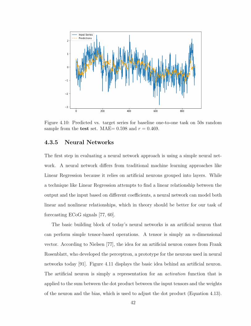
Figure 4.10: Predicted vs. target series for baseline one-to-one task on 50s randomsample from the test set. MAE= 0.598 and r = 0.469.
4.3.5 Neural Networks
The first step in evaluating a neural network approach is using a simple neural net-
work. A neural network differs from traditional machine learning approaches like
Linear Regression because it relies on artificial neurons grouped into layers. While
a technique like Linear Regression attempts to find a linear relationship between the
output and the input based on different coefficients, a neural network can model both
linear and nonlinear relationships, which in theory should be better for our task of
forecasting ECoG signals [77, 60].
The basic building block of today’s neural networks is an artificial neuron that
can perform simple tensor-based operations. A tensor is simply an n-dimensional
vector. According to Nielsen [77], the idea for an artificial neuron comes from Frank
Rosenblatt, who developed the perceptron, a prototype for the neurons used in neural
networks today [91]. Figure 4.11 displays the basic idea behind an artificial neuron.
The artificial neuron is simply a representation for an activation function that is
applied to the sum between the dot product between the input tensors and the weights
of the neuron and the bias, which is used to adjust the dot product (Equation 4.13).
42

Common activation functions include the sigmoid function and the Rectified Linear
Unit (ReLU) because of their nonlinear nature [77, 60, 78].
Figure 4.11: Artificial Neuron. Reproduced from Neural Networks and Deep Learningby Nielsen [77].
output = activation((W × input) + bias) (4.13)
Equation 4.13 highlights the mathematical definition of an artificial neuron, where
W represents the weights of the neuron. The activation function can be conceptual-
ized as determining when the neuron will ”fire” in response to an input, mapping the
neuron’s inputs to values in a specific interval. Because we use nonlinear activation
functions, that means that multiple layers of neurons can be stacked in order to model
nonlinear functions as well [77]. According to Nielsen, this results in networks that
can approximate any function.
In order to learn how to approximate the function that outputs the given tar-
gets based on the given input, a neural network relies on a simple algorithm called
stochastic gradient descent (SGD) [60]. SGD allows the network to learn the approx-
imation of the function by ”computing the gradient of the loss function with regard
to the network’s parameters,” which is also considered a backward pass [60]. The
parameters of the neural network are then moved in opposite direction from the gra-
dient, which reduces the value of the loss on the batch. SGD is further enhanced by
the Backpropagation algorithm which allows the neural network to minimize the loss
function across multiple layers [77, 60]. According to Chollet, most machine learning
43
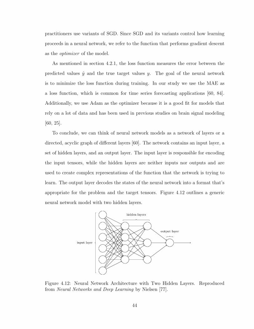
practitioners use variants of SGD. Since SGD and its variants control how learning
proceeds in a neural network, we refer to the function that performs gradient descent
as the optimizer of the model.
As mentioned in section 4.2.1, the loss function measures the error between the
predicted values y and the true target values y. The goal of the neural network
is to minimize the loss function during training. In our study we use the MAE as
a loss function, which is common for time series forecasting applications [60, 84].
Additionally, we use Adam as the optimizer because it is a good fit for models that
rely on a lot of data and has been used in previous studies on brain signal modeling
[60, 25].
To conclude, we can think of neural network models as a network of layers or a
directed, acyclic graph of different layers [60]. The network contains an input layer, a
set of hidden layers, and an output layer. The input layer is responsible for encoding
the input tensors, while the hidden layers are neither inputs nor outputs and are
used to create complex representations of the function that the network is trying to
learn. The output layer decodes the states of the neural network into a format that’s
appropriate for the problem and the target tensors. Figure 4.12 outlines a generic
neural network model with two hidden layers.
Figure 4.12: Neural Network Architecture with Two Hidden Layers. Reproducedfrom Neural Networks and Deep Learning by Nielsen [77].
44

One-to-one Experiment
We first outline the one-to-one baseline neural network experiment. We use a simple
neural network implemented with the Keras deep learning library in order to predict
20 binned steps using a history of length 100 for the electrode with index 5 [92]. The
network has a simple Dense layer consisting of 256 hidden units and uses the Adam
optimizer together with MAE as the loss function [93]. The Dense layer consists of
256 neurons that use no activation function, which was recommended by Chollet for
regression tasks that try to predict an arbitrary value [60]. In addition to the Dense
layer, the model also employs a Flatten layer that transforms all the outputs from the
Dense layer into a single-column tensor that contains all the learned weights. This
layer is fed to another Dense layer that has 20 hidden units (one for each time step
output). The goal of the last Dense layer is to learn how to interpret the weights from
the Flatten layer before it. The output of the Dense layer represents the prediction
of the neural network given the input provided.
The neural network is trained on batches of size 1024 for 100 epochs. If we have
n rows of data in total, an epoch is the process of feeding n/1024 batches to a neural
network, where n/1024 is the number of iterations. Training for a longer period of
times allows the neural network to learn more complex relations within the data.
After training the network, we can evaluate the training and validation loss. This
allows us to track whether the model has been overfitting. When the training loss
becomes higher than the validation loss, we can say that the model has started over-
fitting on the training data. The training vs. validation loss for the one-to-one model
described above can be seen in Figure 4.13.
We notice that the model is able to quickly learn how to interpret the data, since
the difference between the initial and final validation loss is very small. Further-
more, since the loss is relatively constant over 100 epochs, we can also determine
45
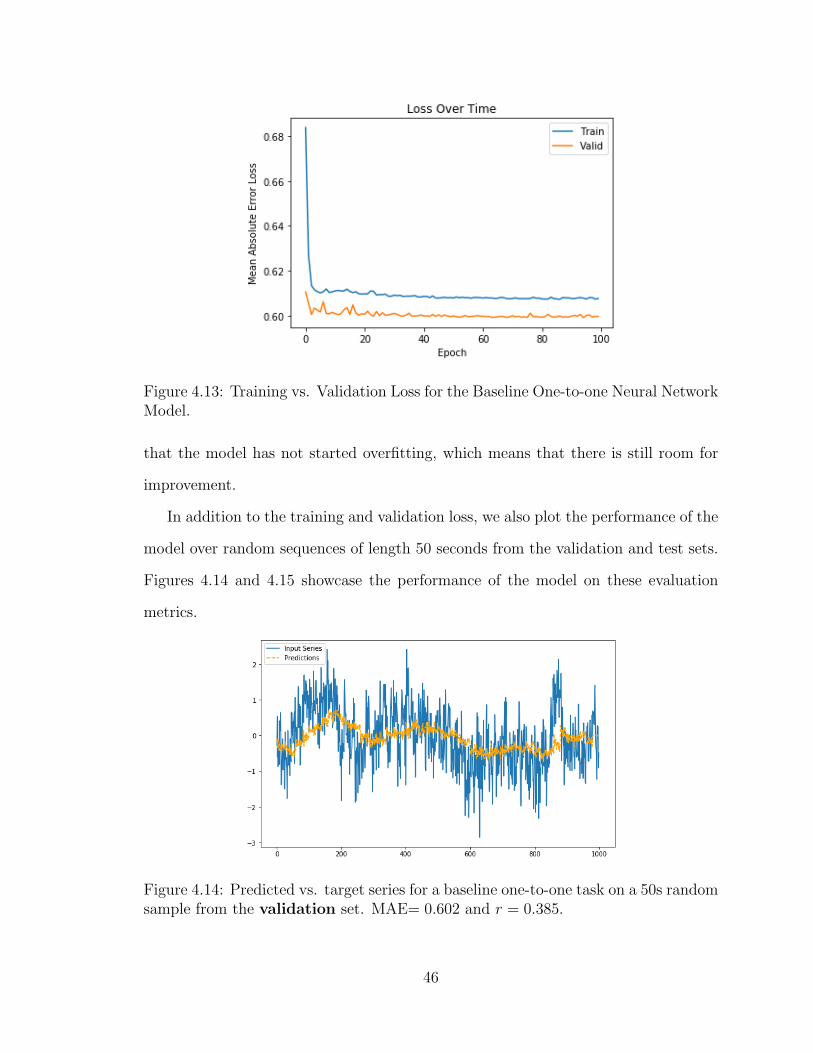
Figure 4.13: Training vs. Validation Loss for the Baseline One-to-one Neural NetworkModel.
that the model has not started overfitting, which means that there is still room for
improvement.
In addition to the training and validation loss, we also plot the performance of the
model over random sequences of length 50 seconds from the validation and test sets.
Figures 4.14 and 4.15 showcase the performance of the model on these evaluation
metrics.
Figure 4.14: Predicted vs. target series for a baseline one-to-one task on a 50s randomsample from the validation set. MAE= 0.602 and r = 0.385.
46
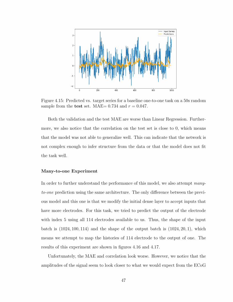
Figure 4.15: Predicted vs. target series for a baseline one-to-one task on a 50s randomsample from the test set. MAE= 0.734 and r = 0.047.
Both the validation and the test MAE are worse than Linear Regression. Further-
more, we also notice that the correlation on the test set is close to 0, which means
that the model was not able to generalize well. This can indicate that the network is
not complex enough to infer structure from the data or that the model does not fit
the task well.
Many-to-one Experiment
In order to further understand the performance of this model, we also attempt many-
to-one prediction using the same architecture. The only difference between the previ-
ous model and this one is that we modify the initial dense layer to accept inputs that
have more electrodes. For this task, we tried to predict the output of the electrode
with index 5 using all 114 electrodes available to us. Thus, the shape of the input
batch is (1024, 100, 114) and the shape of the output batch is (1024, 20, 1), which
means we attempt to map the histories of 114 electrode to the output of one. The
results of this experiment are shown in figures 4.16 and 4.17.
Unfortunately, the MAE and correlation look worse. However, we notice that the
amplitudes of the signal seem to look closer to what we would expect from the ECoG
47
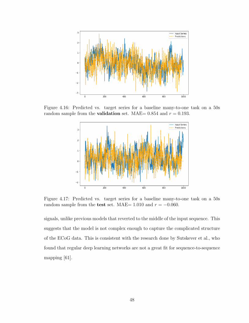
Figure 4.16: Predicted vs. target series for a baseline many-to-one task on a 50srandom sample from the validation set. MAE= 0.854 and r = 0.193.
Figure 4.17: Predicted vs. target series for a baseline many-to-one task on a 50srandom sample from the test set. MAE= 1.010 and r = −0.060.
signals, unlike previous models that reverted to the middle of the input sequence. This
suggests that the model is not complex enough to capture the complicated structure
of the ECoG data. This is consistent with the research done by Sutskever et al., who
found that regular deep learning networks are not a great fit for sequence-to-sequence
mapping [61].
48

4.3.6 Encoder-Decoder Framework
In order to further test our hypothesis that ECoG data can be forecast, we also
employ a sequence-to-sequence encoder-decoder model that utilizes Long Short Term
Memory (LSTM) layers. This model is a better fit for this task and has been inspired
by the work done by Sutskever et al. and Cho et al..
An encoder-model architecture uses two recursive layers in order to map input
sequences of variable length to output sequences of variable length. The first layer is
called the encoder and the second layer is called the decoder. This architecture was
first proposed in 2014 [61, 94]. In our case, we use an encoder-decoder model with
teacher forcing during training. This means that during training we feed the encoder
an input sequence (in our case the history of the ECoG data), which then processes
it. Instead of using the output of the first layer, we throw it away and simply copy the
internal states of the encoder to the second layer, the decoder. Teacher forcing means
that the decoder is fed parts of the target data during training and forced to generate
the next step in the sequence. In our case, the decoder is fed target data that’s
shifted backwards by 1 binned time step, which forces it to learn how to infer the
structure in the signal. During inference, the encoder-decoder model has to generate
output sequences from scratch, using only its previously generated sequences [84].
Our encoder-decoder implementation was inspired by Chollet [95] and Eddy [96].
Encoder-decoder models rely on Recursive Neural Network (RNN) layers. In this
case, we use a specific type of RNN called LSTM [32]. Like RNNs, LSTMs are able to
develop a memory of past actions with the help of an internal state. However, while
RNNs struggle to learn long-term dependencies, LSTMs solve this problem, which is
why we use them in our architecture [60].
We trained an LSTM-based encoder-decoder model on our data in order to better
understand whether a sequence-to-sequence architecture is better at forecasting the
future of an ECoG signal than a baseline neural network. We find that this is the case
49
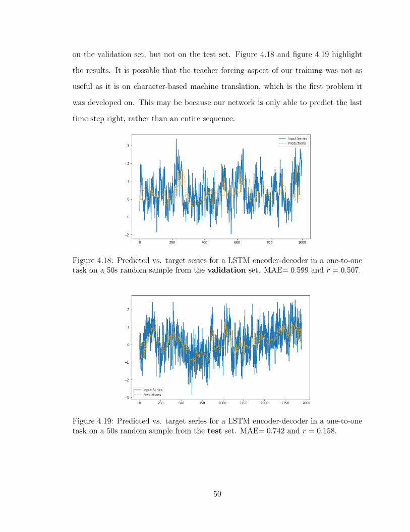
on the validation set, but not on the test set. Figure 4.18 and figure 4.19 highlight
the results. It is possible that the teacher forcing aspect of our training was not as
useful as it is on character-based machine translation, which is the first problem it
was developed on. This may be because our network is only able to predict the last
time step right, rather than an entire sequence.
Figure 4.18: Predicted vs. target series for a LSTM encoder-decoder in a one-to-onetask on a 50s random sample from the validation set. MAE= 0.599 and r = 0.507.
Figure 4.19: Predicted vs. target series for a LSTM encoder-decoder in a one-to-onetask on a 50s random sample from the test set. MAE= 0.742 and r = 0.158.
50

4.3.7 Temporal Convolutional Network
In addition to LSTM, we also attempted to use a Temporal Convolutional Network
(TCN) to forecast ECoG signals. TCNs were first proposed by Bai et al. as a response
to the popularity of recursive-only approaches for sequence-to-sequence modeling.
A TCN differs from previous models because it relies on convolutions rather than
recursive connections. In the context of a TCN for sequence-to-sequence mapping, a
convolutional layer runs a one dimensional filter (also called a kernel) over the input
sequence in order to learn local patterns, while the architectures discussed above
were limited to learning global patterns on the input data. One key aspect of TCNs
is that they use causal convolutions rather than regular convolutions (the kernel is
only applied to time steps before the current one). According to Bai et al., this
prevents leakage from the future to the past.
While convolutional networks were initially developed for tasks related to com-
puter vision, Bai et al. were able to create a lightweight model that can map input
sequences to output sequences. However, a problem with classical convolutions is
that they struggle to learn historical data. The authors were able to overcome this
issue by relying on dilated convolutions and residual connections. Dilated convolu-
tions enable the network to make connections across different combinations of past
data (i.e. a regular one-dimensional convolution sees sequential windows of size k,
while a dilated convolution with d = 2 sees every other window). TCNs embed the
dilated convolutions in residual blocks. A residual block contains two dilated con-
volution layers whose outputs are processed, in sequence, by a weight normalization
layer, a ReLU activation layer, and a Dropout layer. Residual blocks also employ
residual connections that allow the network to learn by skipping residual blocks when
necessary [33].
The advantages of using TCNs compared to recursive neural networks are that
TCNs have a low memory requirement for training and avoid the problem of explod-
51

ing/vanishing gradients [33]. Furthermore, TCNs can be seen as a generic version
of WaveNet. This is an advantage because TCNs enable us to capture some of the
benefits of WaveNet in a lightweight implementation. In our study we used a TCN
implementation adapted from the work of Remy [97].2
We attempted both one-to-one and many-to-one predictions using the TCN ar-
chitecture described above. In order to do so, we set the number of filters used in
the convolutional layers to 32 and the kernel size to 4. In addition to this, we also
used the following dilations: {1, 2, 4, 8, 16}. The list of dilations is equivalent to per-
forming a convolution every window, every other window, every 4th window, and so
forth. This allows the model to learn the relationships between local patterns across
longer sequences. Last but not least, we used 2 stacks of residual blocks given the
complicated nature of the task.
One-to-one Experiment
Similar to previous experiments, we attempted to predict two 50 seconds long se-
quences from the validation and test sets. We forecast the electrode with index 5
using 100 binned time-steps to predict the next 20. The results are shown in figures
4.20 and 4.20.
The TCN results are promising on the validation set, performing just as well as
the LSTM Encoder-Decoder architecture. However, the results on the test set are
not as promising because the correlation drops to near 0 while the MAE is similar.
This indicates that the TCN network does not generalize well on this task.
2GitHub URL: https://github.com/philipperemy/keras-tcn
52

Figure 4.20: Predicted vs. target series for a TCN one-to-one task on a 50s randomsample from the validation set. MAE= 0.585 and r = 0.449.
Figure 4.21: Predicted vs. target series for a TCN one-to-one task on a 50s randomsample from the test set. MAE= 0.740 and r = 0.015.
Many-to-one Experiment
In addition to the one-to-one task, we also attempt a many-to-one prediction using
the same parameters. The only difference is that we use the histories of all 114
electrodes rather than just the history of electrode 5. The results are shown in figures
4.22 and 4.23.
The results from the many-to-one TCN experiment show that adding more in-
formation from multiple electrodes does not improve our ability to predict the data.
53

Figure 4.22: Predicted vs. target series for a TCN many-to-one task on a 50s randomsample from the validation set. MAE= 0.672 and r = 0.163.
Figure 4.23: Predicted vs. target series for a TCN many-to-one task on a 50s randomsample from the test set. MAE= 0.771 and r = 0.113.
Furthermore, it seems that the additional data has a negative effect, since the exper-
iment ran on the validation set does worse in terms of MAE than the test set.
4.3.8 WaveNet
The last model used in this study is WaveNet. WaveNet was developed by Google
DeepMind to generate raw audio waveforms [34]. This model is more advanced than
the TCN model discussed above because it includes skip connections across layers,
conditioning, context stacking, and gated activations [33]. However, it is still based
54

on the Convolutional Neural Network (CNN) architecture. WaveNet represents one
of the top models for generating raw audio from scratch, including music [34]. In this
study, we ran a slightly modified version of WaveForm as implemented by Eddy [96].3
Similar to previous models, we compared the one-to-one and many-to-one pre-
diction tasks. Similar to the TCN model, we initialized the WaveNet model with 32
filters of width 2. One difference between WaveNet and TCN is that we used more
dilations in this model: {1, 2, 4, 8, 16, 32, 64, 128}.
The task for the one-to-one experiment was the same as outlined above. The
results are shown in Figure 4.24 and 4.25. Similarly, results for the many-to-one
experiment are shown in Figure 4.26 and 4.8.
Figure 4.24: Predicted vs. target series for a WaveNet one-to-one task on a 50srandom sample from the validation set. MAE= 0.572 and r = 0.504.
The results produced by WaveNet are the most promising compared to our other
models. For one-to-one forecasting, WaveNet consistently outperforms the other
models when comparing the results for the validation set. However, the test set
paints a different picture. Like previous neural network models, WaveNet is not
able to generalize either and comes in last, although its correlation is slightly better
compared to the other neural network models.
3GitHub URL: https://github.com/JEddy92/TimeSeries Seq2Seq
55

Figure 4.25: Predicted vs. target series for a WaveNet one-to-one task on a 50srandom sample from the test set. MAE= 0.744 and r = 0.175.
Figure 4.26: Predicted vs. target series for a WaveNet many-to-one task on a 50srandom sample from the validation set. MAE= 0.572 and r = 0.504.
On the many-to-one task, WaveNet outperforms other neural network models
in terms of MAE and correlation on sequences from the validation and test sets.
However, like other neural network based approaches, using multiple electrodes does
not yield an increase in performance. Thus, the many-to-one WaveNet is not able to
beat the one-to-one linear regression in the task to forecast ECoG signals.
56

Figure 4.27: Predicted vs. target series for a WaveNet many-to-one task on a 50srandom sample from the test set. MAE= 0.744 and r = 0.175.
4.4 Complete Results
This section contains the complete results from the experiments performed in the
previous section. All results are outlined in Table 4.3 and Table 4.4. Note that
the Linear Regression result in Table 4.4 is the same as the one in Table 4.3. This
is because we use one-to-one Linear Regression to benchmark our performance and
verify the hypothesis that neural networks that have access to more electrodes will be
able to model the structure of the activity in the brain better than simpler models.
ExperimentDescription
MAE(Validation)
Correlation(Validation)
MAE(Test)
Correlation(Test)
Baseline InputShifting
0.871 0.005 0.825 -0.014
Linear Regression 0.577 0.479 0.469 0.598Baseline Neural
Network0.602 0.385 0.734 0.047
LSTM Encoder-Decoder
with Teacher Forcing0.580 0.484 0.742 0.158
Temporal ConvolutionalNetwork
0.585 0.449 0.740 0.0156
WaveNet 0.572 0.504 0.744 0.175
Table 4.3: One-to-one Validation and Testing Results
57

ExperimentDescription
MAE(Validation)
Correlation(Validation)
MAE(Test)
Correlation(Test)
Linear Regression Baseline(One-to-one)
0.577 0.479 0.469 0.598
Baseline NeuralNetwork
0.854 0.194 1.01 -0.060
Temporal ConvolutionalNetwork
0.672 0.163 0.771 0.10
WaveNet 0.641 0.378 0.747 0.113
Table 4.4: Many-to-one Validation and Testing Results
Our results show that predicting ECoG electrode signals can be done with varying
degrees of success. While our models perform well when predicting specific samples,
the results on the test set highlight that we are still far away from a generalizable
solution. An interesting aspect of the results is that using more electrodes does not
seem to help our prediction task. Both validation and test set results for many-to-one
prediction are worse than for one-to-one prediction.
We also note the relatively similar performance of the models in terms of MAE on
each individual set. For instance, all neural-network based approaches in Table 4.3
are within 0.030 of each other in the validation set and within 0.012 in the test set.
This suggests that a performance bottleneck is quickly encountered by all models.
This is further discussed in Section 5.1.
Another noteworthy aspect about the results is that Linear Regression, a simpler
model, is able to achieve similar if not better performance than WaveNet. This is
surprising given the complex nature of the data, but could also point to the possibility
that deep learning might not be the best way to model these signals.
The performance of the deep learning models on the validation set compared to
the test set also suggests that our manual hyper-parameter optimization might have
led to slight overfitting, although this is not reflected in the training vs. validation
loss graphs generated for each model during training.
58

Nevertheless, the results outlined above highlight that we were able to meet our
research goals in several ways. First, we were able to use neural networks to extract
trends from future data, which could be used to provide context speech decoding
models like the ones developed by Moses et al. [24]. Second, the trends extracted
by our models could be used by neuroscientists to better understand how the areas
responsible for speech work. Third, since our ECoG data is synchronized with free-
flowing speech we might be able to increase the robustness of speech decoding models.
This aspect is further discussed in Section 5.1.
4.5 Limitations
There are several limitations associated with the current work. Chief among them
is electrode selection. This is because we did not run all the models mentioned in
Section 4.3 on all electrodes in an exhaustive manner. Instead, we selected an elec-
trode based on its performance on linear regression and the common-sense approach
described in section 4.3.2. In our case, the electrode being monitored achieved one
of the lowest MAEs and correlations across all other 114, which made it a good can-
didate for other one-to-one and many-to-one tests. Nevertheless, it is possible that
we chose an electrode that is particularly well-suited for Linear Regression but is not
representative of other electrodes. Similarly, it is possible that the electrode was not
particularly informative in terms of signal-to-noise ratio or that one electrode does
not carry enough signal for this task.
Additionally, exhaustive hyper-parameter optimization was not performed on the
deep learning models used in this study. We attempted using libraries like Wandb [98]
and Hyper-Opt [99], but the MAE score did not prove to be a good enough evaluation
metric to help us find better parameters. This is because the MAE quickly plateaus
during training and stays constant afterwards in relation to this task. It is possible
59

that by using a better evaluation metric we might be able to make more extensive
use of these libraries.
It is also possible that the patient being monitored was not a great fit for this
study. While we analyzed different electrodes across multiple patients in this study
and selected the electrode with index 5 according to performance on baseline models,
we have no information on the health of the patient and whether there are any
physiological factors that might make others a better fit for this study.
60

Chapter 5
Discussion, Future Work, and
Conclusion
5.1 Discussion and Future Work
Our results are promising because they show that forecasting ECoG signals is not
impossible. However, there is still a lot of work to be done in this research area.
While our deep learning models did not perform as expected on the test set, we have
noticed that it is possible to predict the overall trend of the signal, which was one of
the goals of this study.
While brain-to-speech forecasting might not be possible given the performance of
our metrics outlined above, the models developed could be repurposed to improve
speech synthesis from the brain. For instance, one important area of future work is
using the trends generated by the machine learning models discussed above in order
to enhance the functionality and performance of speech neuroprostheses and brain-
to-speech systems like the ones described by Makin et al., Anumanchipalli et al., and
Moses et al..
61

Another avenue for future work is improving current speech prostheses that depend
on technologies like eye tracking or modified computer peripherals using the methods
described above. For example, the trends collected and interpreted by an ECoG or
EEG model could be used to augment text using some form of emotions. While
not perfect, this would increase the expressivity of current devices and pave the way
for the increased adoption of invasive brain-computer interfaces by showcasing their
benefits.
We have noticed that the models used in this work were overwhelmed by the data
provided to them, especially since the many-to-one task showed worse results than
the one-to-one task. Therefore, another important aspect of future work is using
deeper network architectures. Besides WaveNet, most of the networks used in the
study were relatively shallow.
The results also highlight the importance of hyper-parameter optimization. Using
the right loss function or optimizer can have a strong impact on the results. While
we used Adam and MAE, it is possible that other optimizers or loss functions might
provide an easier way for the neural network model to learn the specific amplitudes
in the data. Furthermore, details like the number of hidden units, the size of the
kernel, and the number of dilations can also have a strong impact on the performance
of the models. This is why an exhaustive hyper-parameter search using a library like
Wandb or Hyper-Opt could make an important difference [98, 99].
It is also possible that the ECoG signals used might contain too many concurrent
signals to properly predict them. As a result, it might be useful to add a downstream
validation task in order to guide the neural network towards extracting a specific type
of signal from the input data for the purpose of sequence-to-sequence prediction. For
example, we could leverage the audio waveforms from speech to create a model that
attempts speech synthesis and signal forecasting simultaneously. This could allow
62

the neural network to better understand the relationship between the signals and
differentiate the signal relevant signal from the noise.
Another aspect of this study that could be improved is using normalized data
instead of binned data. Binned data is downsampled and is an average of the signal
found in the normalized data, which could reduce the amount of useful information
that is fed to the neural network. One caveat to this note is that we attempted to
forecast normalized data, but one of the issues we ran into is that the neural network
models had trouble converging in many instances.
Last but not least, our forecasting approach could also be improved. Rather than
attempting to predict full sequences, the problem could be simplified by focusing
on predicting single data points in the future. This might be more adequate for
the models described in Section 4.3 and could provide an easier starting point. After
obtaining good results with forecasting singular time steps at different delays, it might
be easier to find a way to forecast full sequences.
5.2 Conclusion
Our work highlights the difficult nature of ECoG time series forecasting. We build on
the work of other speech neuroprosthesis researchers in order to develop models that
can forecast ECoG signals from real patients. Our goal is to find models that can
forecast these signals so that they can be used for applications in speech forecasting,
context and performance improvement for current brain-to-speech decoder models,
and neuroscience.
We show that WaveNet is the most promising deep learning model tested, but
forecasting results are mixed. While some samples can be easily predicted, others
remain elusive. Furthermore, we also find that using multiple electrodes to predict
63

the signal of one does not improve the performance of the models. Last but not least,
we find that simpler models like linear regression can do surprisingly well on this task.
We also suggest several areas of future work. One of them is related to using the
fact that neural network models like the Long Short-Term Memory (LSTM) Encoder-
Decoder model, the Temporal Convolutional Network (TCN) model, and WaveNet
can capture the trend of the signal relatively well. This can improve speech synthesis
by providing more context to the decoding models.
We also propose a way to improve ECoG signal forecasting. We reason that it is
possible that the ECoG signals used in this study encode multiple signals related to
movement, speech, and other activities related to brain activation. As a result of this,
forecasting ECoG signals may be impossible because they encode multiple activities
simultaneously. In order to overcome this problem, we suggest using a downstream
prediction task to ”guide” the neural network model during training, similar to the
model used by Makin et al. [25]. An example of such a task is forcing the neural
network to predict both ECoG brain signals and audio waveforms in parallel. During
inference, the neural network would simply use the states gained from attempting
to predict speech in order to predict ECoG signals. We believe that this approach
might reduce the complexity of the problem, allowing us to better understand speech
generation and production in the human brain but also forecast it in a reliable way.
Doing so will allow us to unlock superpowers not available to any humans before us.
64

Appendix A
Code Availability
The code used to implement and test the models referenced in this work is available
at: https://github.com/theodormarcu/brain2brain
65

Bibliography
[1] K. A. Moxon and G. Foffani, “Brain-machine interfaces beyond neuroprosthet-ics,” Neuron, vol. 86, no. 1, pp. 55–67, 2015.
[2] G. Schalk, D. J. McFarland, T. Hinterberger, N. Birbaumer, and J. R. Wol-paw, “Bci2000: a general-purpose brain-computer interface (bci) system,” IEEETransactions on Biomedical Engineering, vol. 51, no. 6, pp. 1034–1043, 2004.
[3] J. R. Wolpaw, N. Birbaumer, W. J. Heetderks, D. J. McFarland, P. H. Peckham,G. Schalk, E. Donchin, L. A. Quatrano, C. J. Robinson, and T. M. Vaughan,“Brain-computer interface technology: a review of the first international meet-ing,” IEEE transactions on rehabilitation engineering, vol. 8, no. 2, pp. 164–173,2000.
[4] D. Coyle, Brain-Computer Interfaces: Lab Experiments to Real-WorldApplications, ser. ISSN. Elsevier Science, 2016. [Online]. Available: https://books.google.com/books?id=b3i0CwAAQBAJ
[5] L. Garcia, V. Lespinet-Najib, M. Menoret, B. Claverie, J. M. Andr, andR. Ron-Angevin, “Chapter 69 - braincomputer interface: Analysis of differentvirtual keyboards for improving usability,” in Neuroergonomics, H. Ayaz andF. Dehais, Eds. Academic Press, 2018, pp. 269 – 270. [Online]. Available:http://www.sciencedirect.com/science/article/pii/B9780128119266000695
[6] P. R. Kennedy and R. A. Bakay, “Restoration of neural output from a paralyzedpatient by a direct brain connection,” Neuroreport, vol. 9, no. 8, pp. 1707–1711,1998.
[7] P. R. Kennedy, R. A. Bakay, M. M. Moore, K. Adams, and J. Goldwaithe,“Direct control of a computer from the human central nervous system,” IEEETransactions on rehabilitation engineering, vol. 8, no. 2, pp. 198–202, 2000.
[8] A. Kubler, A. Furdea, S. Halder, E. M. Hammer, F. Nijboer, and B. Kotchoubey,“A brain–computer interface controlled auditory event-related potential (p300)spelling system for locked-in patients,” Annals of the New York Academy ofSciences, vol. 1157, no. 1, pp. 90–100, 2009.
[9] J. R. Wolpaw, D. J. McFarland, G. W. Neat, and C. A. Forneris, “An eeg-basedbrain-computer interface for cursor control,” Electroencephalography and clinicalneurophysiology, vol. 78, no. 3, pp. 252–259, 1991.
66

[10] E. E. Fetz, “Operant conditioning of cortical unit activity,” Science, vol. 163,no. 3870, pp. 955–958, 1969.
[11] ——, “Volitional control of neural activity: implications for brain–computer in-terfaces,” The Journal of physiology, vol. 579, no. 3, pp. 571–579, 2007.
[12] V. Vinge, “Technological singularity,” in VISION-21 Symposium sponsored byNASA Lewis Research Center and the Ohio Aerospace Institute, 1993, pp. 30–31.
[13] N. Bostrom and A. Sandberg, “Cognitive enhancement: methods, ethics, regu-latory challenges,” Science and engineering ethics, vol. 15, no. 3, pp. 311–341,2009.
[14] S. Bavishi, J. Rosenthal, and M. Bockbrader, “Chapter 17 - neuroprosthetics,”in Rehabilitation After Traumatic Brain Injury, B. C. Eapen and D. X.Cifu, Eds. Elsevier, 2019, pp. 241 – 253. [Online]. Available: http://www.sciencedirect.com/science/article/pii/B9780323544566000177
[15] J. S. Brumberg, K. M. Pitt, and J. D. Burnison, “A noninvasive brain-computerinterface for real-time speech synthesis: The importance of multimodal feed-back,” IEEE Transactions on Neural Systems and Rehabilitation Engineering,vol. 26, no. 4, pp. 874–881, 2018.
[16] P. Nuyujukian, J. A. Sanabria, J. Saab, C. Pandarinath, B. Jarosiewicz, C. H.Blabe, B. Franco, S. T. Mernoff, E. N. Eskandar, J. D. Simeral et al., “Corticalcontrol of a tablet computer by people with paralysis,” PloS one, vol. 13, no. 11,2018.
[17] G. K. Anumanchipalli, J. Chartier, and E. F. Chang, “Speech synthesis fromneural decoding of spoken sentences,” Nature, vol. 568, no. 7753, pp. 493–498,2019.
[18] S. Koch Fager, M. Fried-Oken, T. Jakobs, and D. R. Beukelman, “New andemerging access technologies for adults with complex communication needs andsevere motor impairments: State of the science,” Augmentative and AlternativeCommunication, vol. 35, no. 1, pp. 13–25, 2019.
[19] E. F. Chang and G. K. Anumanchipalli, “Toward a speech neuroprosthesis,”Jama, vol. 323, no. 5, pp. 413–414, 2020.
[20] J. S. Brumberg, P. R. Kennedy, and F. H. Guenther, “Artificial speech synthe-sizer control by brain-computer interface,” in Tenth Annual Conference of theInternational Speech Communication Association, 2009.
[21] J. S. Brumberg, E. J. Wright, D. S. Andreasen, F. H. Guenther, and P. R.Kennedy, “Classification of intended phoneme production from chronic intra-cortical microelectrode recordings in speech motor cortex,” Frontiers in neuro-science, vol. 5, p. 65, 2011.
67

[22] X. Pei, D. L. Barbour, E. C. Leuthardt, and G. Schalk, “Decoding vowels andconsonants in spoken and imagined words using electrocorticographic signals inhumans,” Journal of neural engineering, vol. 8, no. 4, p. 046028, 2011.
[23] C. Herff, D. Heger, A. De Pesters, D. Telaar, P. Brunner, G. Schalk, andT. Schultz, “Brain-to-text: decoding spoken phrases from phone representationsin the brain,” Frontiers in neuroscience, vol. 9, p. 217, 2015.
[24] D. A. Moses, M. K. Leonard, J. G. Makin, and E. F. Chang, “Real-time decodingof question-and-answer speech dialogue using human cortical activity,” Naturecommunications, vol. 10, no. 1, pp. 1–14, 2019.
[25] J. G. Makin, D. A. Moses, and E. F. Chang, “Machine translation of corticalactivity to text with an encoder–decoder framework,” Nature Publishing Group,Tech. Rep., 2020.
[26] B. Blaus, “Blausen. com staff (2014),,” Medical gallery of Blausen Medical, 2014.
[27] A. Wrench, “The mocha-timit articulatory database,” 1999.
[28] M. Angrick, C. Herff, E. Mugler, M. C. Tate, M. W. Slutzky, D. J. Krusienski,and T. Schultz, “Speech synthesis from ecog using densely connected 3d convo-lutional neural networks,” Journal of neural engineering, vol. 16, no. 3, 2019.
[29] A. A. Wrench, “A multichannel articulatory database and its application forautomatic speech recognition,” in In Proceedings 5 th Seminar of Speech Pro-duction. Citeseer, 2000.
[30] N. Kriegeskorte, “Deep neural networks: a new framework for modeling biologicalvision and brain information processing,” Annual review of vision science, vol. 1,pp. 417–446, 2015.
[31] A. Kuruvilla and R. Flink, “Intraoperative electrocorticography in epilepsysurgery: useful or not?” Seizure, vol. 12, no. 8, pp. 577–584, 2003.
[32] S. Hochreiter and J. Schmidhuber, “Lstm can solve hard long time lag problems,”in Advances in neural information processing systems, 1997, pp. 473–479.
[33] S. Bai, J. Z. Kolter, and V. Koltun, “An empirical evaluation of genericconvolutional and recurrent networks for sequence modeling,” CoRR, vol.abs/1803.01271, 2018. [Online]. Available: http://arxiv.org/abs/1803.01271
[34] A. v. d. Oord, S. Dieleman, H. Zen, K. Simonyan, O. Vinyals, A. Graves,N. Kalchbrenner, A. Senior, and K. Kavukcuoglu, “Wavenet: A generative modelfor raw audio,” arXiv preprint arXiv:1609.03499, 2016.
[35] N. E. Crone, A. Sinai, and A. Korzeniewska, “High-frequency gamma oscillationsand human brain mapping with electrocorticography,” Progress in brain research,vol. 159, pp. 275–295, 2006.
68

[36] K. Volkova, M. A. Lebedev, A. Kaplan, and A. Ossadtchi, “Decoding movementfrom electrocorticographic activity: A review,” Frontiers in Neuroinformatics,vol. 13, 2019.
[37] J. Yeo, M. Youssef, and A. Agrawala, “A framework for wireless lan monitor-ing and its applications,” in Proceedings of the 3rd ACM workshop on Wirelesssecurity, 2004, pp. 70–79.
[38] M. Schulz, P. Klapper, M. Hollick, E. Tews, and S. Katzenbeisser, “Trust thewire, they always told me! on practical non-destructive wire-tap attacks againstethernet,” in Proceedings of the 9th ACM Conference on Security & Privacy inWireless and Mobile Networks, 2016, pp. 43–48.
[39] E. S. Nurse, S. E. John, D. R. Freestone, T. J. Oxley, H. Ung, S. F. Berkovic, T. J.O’Brien, M. J. Cook, and D. B. Grayden, “Consistency of long-term subduralelectrocorticography in humans,” IEEE Transactions on Biomedical Engineering,vol. 65, no. 2, pp. 344–352, 2017.
[40] V. Gilja, C. Pandarinath, C. H. Blabe, P. Nuyujukian, J. D. Simeral, A. A.Sarma, B. L. Sorice, J. A. Perge, B. Jarosiewicz, L. R. Hochberg et al., “Clinicaltranslation of a high-performance neural prosthesis,” Nature medicine, vol. 21,no. 10, p. 1142, 2015.
[41] B. Jarosiewicz, A. A. Sarma, D. Bacher, N. Y. Masse, J. D. Simeral, B. Sorice,E. M. Oakley, C. Blabe, C. Pandarinath, V. Gilja et al., “Virtual typing by peoplewith tetraplegia using a self-calibrating intracortical brain-computer interface,”Science translational medicine, vol. 7, no. 313, pp. 313ra179–313ra179, 2015.
[42] C. Kapeller, P. Gergondet, K. Kamada, H. Ogawa, F. Takeuchi, R. Ortner,R. Prueckl, A. Kheddar, J. Scharinger, and C. Guger, “Online control of a hu-manoid robot through hand movement imagination using csp and ecog basedfeatures,” in 2015 37th Annual International Conference of the IEEE Engineer-ing in Medicine and Biology Society (EMBC). IEEE, 2015, pp. 1765–1768.
[43] R. K. Shepherd, M. N. Shivdasani, D. A. Nayagam, C. E. Williams, and P. J.Blamey, “Visual prostheses for the blind,” Trends in biotechnology, vol. 31,no. 10, pp. 562–571, 2013.
[44] A. P. Finn, D. S. Grewal, and L. Vajzovic, “Argus ii retinal prosthesis system:a review of patient selection criteria, surgical considerations, and post-operativeoutcomes,” Clinical ophthalmology (Auckland, NZ), vol. 12, p. 1089, 2018.
[45] P. Ghasemi, T. Sahraee, and A. Mohammadi, “Closed-and open-loop deepbrain stimulation: methods, challenges, current and future aspects,” Journalof biomedical physics & engineering, vol. 8, no. 2, p. 209, 2018.
[46] A. Fasano, A. Daniele, and A. Albanese, “Treatment of motor and non-motorfeatures of parkinson’s disease with deep brain stimulation,” The Lancet Neurol-ogy, vol. 11, no. 5, pp. 429–442, 2012.
69

[47] G. K. Bergey, M. J. Morrell, E. M. Mizrahi, A. Goldman, D. King-Stephens,D. Nair, S. Srinivasan, B. Jobst, R. E. Gross, D. C. Shields et al., “Long-termtreatment with responsive brain stimulation in adults with refractory partialseizures,” Neurology, vol. 84, no. 8, pp. 810–817, 2015.
[48] H. S. Mayberg, A. M. Lozano, V. Voon, H. E. McNeely, D. Seminowicz,C. Hamani, J. M. Schwalb, and S. H. Kennedy, “Deep brain stimulation fortreatment-resistant depression,” Neuron, vol. 45, no. 5, pp. 651–660, 2005.
[49] J. D. Kropotov, “Chapter 4.2 - neurofeedback,” in Functional Neuromarkersfor Psychiatry, J. D. Kropotov, Ed. San Diego: Academic Press, 2016, pp.247 – 266. [Online]. Available: http://www.sciencedirect.com/science/article/pii/B9780124105133000164
[50] T. Brandmeyer and A. Delorme, “Meditation and neurofeedback,” Frontiers inpsychology, vol. 4, p. 688, 2013.
[51] J. Bu, K. D. Young, W. Hong, R. Ma, H. Song, Y. Wang, W. Zhang, M. Hamp-son, T. Hendler, and X. Zhang, “Effect of deactivation of activity patterns re-lated to smoking cue reactivity on nicotine addiction,” Brain, vol. 142, no. 6, pp.1827–1841, 2019.
[52] J. F. Lubar, “Neurofeedback for the management of attention deficit disorders.”2003.
[53] L. Oberman and A. Pascual-Leone, “Chapter 4 - changes in plasticity acrossthe lifespan: Cause of disease and target for intervention,” in Changing Brains,ser. Progress in Brain Research, M. M. Merzenich, M. Nahum, and T. M. V.Vleet], Eds. Elsevier, 2013, vol. 207, pp. 91 – 120. [Online]. Available:http://www.sciencedirect.com/science/article/pii/B9780444633279000163
[54] M. Akcakaya, B. Peters, M. Moghadamfalahi, A. R. Mooney, U. Orhan, B. Oken,D. Erdogmus, and M. Fried-Oken, “Noninvasive brain–computer interfaces foraugmentative and alternative communication,” IEEE reviews in biomedical en-gineering, vol. 7, pp. 31–49, 2013.
[55] J. R. Wolpaw, N. Birbaumer, D. J. McFarland, G. Pfurtscheller, and T. M.Vaughan, “Brain–computer interfaces for communication and control,” Clinicalneurophysiology, vol. 113, no. 6, pp. 767–791, 2002.
[56] U. Orhan, K. E. Hild, D. Erdogmus, B. Roark, B. Oken, and M. Fried-Oken,“Rsvp keyboard: An eeg based typing interface,” in 2012 IEEE InternationalConference on Acoustics, Speech and Signal Processing (ICASSP). IEEE, 2012,pp. 645–648.
[57] B. Peters, M. Higger, F. Quivira, S. Bedrick, S. Dudy, B. Eddy, M. Kinsella,T. Memmott, J. Wiedrick, M. Fried-Oken et al., “Effects of simulated visual
70
acuity and ocular motility impairments on ssvep brain-computer interface per-formance: an experiment with shuffle speller,” Brain-Computer Interfaces, vol. 5,no. 2-3, pp. 58–72, 2018.
[58] M. J. Sjerps, N. P. Fox, K. Johnson, and E. F. Chang, “Speaker-normalizedsound representations in the human auditory cortex,” Nature communications,vol. 10, no. 1, pp. 1–9, 2019.
[59] H. G. Yi, M. K. Leonard, and E. F. Chang, “The encoding of speechsounds in the superior temporal gyrus,” Neuron, vol. 102, no. 6, pp. 1096 –1110, 2019. [Online]. Available: http://www.sciencedirect.com/science/article/pii/S0896627319303800
[60] F. Chollet, Deep Learning with Python, 1st ed. USA: Manning PublicationsCo., 2017.
[61] I. Sutskever, O. Vinyals, and Q. V. Le, “Sequence to sequence learning withneural networks,” in Advances in neural information processing systems, 2014,pp. 3104–3112.
[62] C. Pandarinath, P. Nuyujukian, C. H. Blabe, B. L. Sorice, J. Saab, F. R.Willett, L. R. Hochberg, K. V. Shenoy, and J. M. Henderson, “Highperformance communication by people with paralysis using an intracorticalbrain-computer interface,” eLife, vol. 6, p. e18554, feb 2017. [Online]. Available:https://doi.org/10.7554/eLife.18554
[63] Y. Jeon, C. S. Nam, Y.-J. Kim, and M. C. Whang, “Event-related (de) synchro-nization (erd/ers) during motor imagery tasks: Implications for brain–computerinterfaces,” International Journal of Industrial Ergonomics, vol. 41, no. 5, pp.428–436, 2011.
[64] L. H. Arnal, D. Poeppel, and A.-L. Giraud, “A neurophysiological perspective onspeech processing in the neurobiology of language,” in Neurobiology of language.Elsevier, 2016, pp. 463–478.
[65] A. Llorens, A. Trebuchon, C. Liegeois-Chauvel, F. Alario et al., “Intra-cranialrecordings of brain activity during language production,” Frontiers in psychology,vol. 2, p. 375, 2011.
[66] N. Crone, L. Hao, J. Hart, D. Boatman, R. P. Lesser, R. Irizarry, and B. Gordon,“Electrocorticographic gamma activity during word production in spoken andsign language,” Neurology, vol. 57, no. 11, pp. 2045–2053, 2001.
[67] N. E. Crone and L. Hao, “Functional dynamics of spoken and signedword production: A case study using electrocorticographic spectral analysis,”Aphasiology, vol. 16, no. 9, pp. 903–927, 2002. [Online]. Available:https://doi.org/10.1080/02687030244000383
71

[68] R. T. Canolty, M. Soltani, S. S. Dalal, E. Edwards, N. F. Dronkers, S. S. Nagara-jan, H. E. Kirsch, N. M. Barbaro, and R. T. Knight, “Spatiotemporal dynamicsof word processing in the human brain,” Frontiers in neuroscience, vol. 1, p. 14,2007.
[69] V. L. Towle, H.-A. Yoon, M. Castelle, J. C. Edgar, N. M. Biassou, D. M. Frim,J.-P. Spire, and M. H. Kohrman, “Ecog gamma activity during a language task:differentiating expressive and receptive speech areas,” Brain, vol. 131, no. 8, pp.2013–2027, 2008.
[70] R. P. Lesser, N. E. Crone, and W. Webber, “Subdural electrodes,” Clinical neu-rophysiology, vol. 121, no. 9, pp. 1376–1392, 2010.
[71] R. Cooper, A. Winter, H. Crow, and W. G. Walter, “Comparison of subcorti-cal, cortical and scalp activity using chronically indwelling electrodes in man,”Electroencephalography and clinical neurophysiology, vol. 18, no. 3, pp. 217–228,1965.
[72] U. Hason, A. Goldstein, Z. Zada, E. Ham, C. Kim, and G. Choe, “Hasson Lab,Princeton Neuroscience Institute.”
[73] K. A. Ludwig, R. M. Miriani, N. B. Langhals, M. D. Joseph, D. J. Anderson,and D. R. Kipke, “Using a common average reference to improve cortical neuronrecordings from microelectrode arrays,” Journal of neurophysiology, vol. 101,no. 3, pp. 1679–1689, 2009.
[74] J. O. Smith, Spectral Audio Signal Processing. Website, accessed May 1, 2020,online book, 2011 edition.
[75] U. D. S. Processing, “Unit 6: Windowing,” https://www.phon.ucl.ac.uk/courses/spsci/dsp/window.html, [Online; accessed 01-May-2020].
[76] Y. A. LeCun, L. Bottou, G. B. Orr, and K.-R. Muller, “Efficient backprop,” inNeural networks: Tricks of the trade. Springer, 2012, pp. 9–48.
[77] M. A. Nielsen, Neural networks and deep learning. Determination press SanFrancisco, CA, USA, 2015, vol. 2018.
[78] I. Goodfellow, Y. Bengio, and A. Courville, Deep Learning. MIT Press, 2016,http://www.deeplearningbook.org.
[79] K. P. Murphy, Machine learning: a probabilistic perspective. MIT press, 2012.
[80] Z. Mariet and V. Kuznetsov, “Foundations of sequence-to-sequence modeling fortime series,” in The 22nd International Conference on Artificial Intelligence andStatistics, 2019, pp. 408–417.
[81] P. J. Brockwell, R. A. Davis, and S. E. Fienberg, Time series: theory and meth-ods: theory and methods. Springer Science & Business Media, 1991.
72

[82] J. H. Stock and M. W. Watson, “Vector autoregressions,” Journal of Economicperspectives, vol. 15, no. 4, pp. 101–115, 2001.
[83] L. Zhu and N. Laptev, “Deep and confident prediction for time series at uber,”in 2017 IEEE International Conference on Data Mining Workshops (ICDMW).IEEE, 2017, pp. 103–110.
[84] T. Chai and R. R. Draxler, “Root mean square error (rmse) or mean absoluteerror (mae)?–arguments against avoiding rmse in the literature,” Geoscientificmodel development, vol. 7, no. 3, pp. 1247–1250, 2014.
[85] R. J. Hyndman and A. B. Koehler, “Another look at measures of forecast accu-racy,” International journal of forecasting, vol. 22, no. 4, pp. 679–688, 2006.
[86] J. Lee Rodgers and W. A. Nicewander, “Thirteen ways to look at the correlationcoefficient,” The American Statistician, vol. 42, no. 1, pp. 59–66, 1988.
[87] P. Virtanen, R. Gommers, T. E. Oliphant, M. Haberland, T. Reddy, D. Cour-napeau, E. Burovski, P. Peterson, W. Weckesser, J. Bright et al., “Scipy 1.0:fundamental algorithms for scientific computing in python,” Nature methods,vol. 17, no. 3, pp. 261–272, 2020.
[88] A. Amidi and S. Amidi. (2017) A detailed example of how to use datagenerators with keras. [Online]. Available: https://stanford.edu/∼shervine/blog/keras-how-to-generate-data-on-the-fly
[89] S. van der Walt, S. C. Colbert, and G. Varoquaux, “The numpy array: A struc-ture for efficient numerical computation,” Computing in Science Engineering,vol. 13, no. 2, pp. 22–30, March 2011.
[90] F. Pedregosa, G. Varoquaux, A. Gramfort, V. Michel, B. Thirion, O. Grisel,M. Blondel, P. Prettenhofer, R. Weiss, V. Dubourg et al., “Scikit-learn: Machinelearning in python,” the Journal of machine Learning research, vol. 12, pp. 2825–2830, 2011.
[91] F. Rosenblatt, “Principles of neurodynamics. perceptrons and the theory of brainmechanisms,” Cornell Aeronautical Lab Inc Buffalo NY, Tech. Rep., 1961.
[92] F. Chollet et al., “Keras,” https://keras.io, 2015.
[93] D. P. Kingma and J. Ba, “Adam: A method for stochastic optimization,” arXivpreprint arXiv:1412.6980, 2014.
[94] K. Cho, B. Van Merrienboer, C. Gulcehre, D. Bahdanau, F. Bougares,H. Schwenk, and Y. Bengio, “Learning phrase representations using rnn encoder-decoder for statistical machine translation,” arXiv preprint arXiv:1406.1078,2014.
73

[95] F. Chollet, “A ten-minute introduction to sequence-to-sequence learning in keras,” Available at https://blog.keras.io/a-ten-minute-introduction-to-sequence-to-sequence-learning-in-keras.html(2017/09/29).
[96] J. Eddy, “Time series seq2seq,” Available at https://github.com/JEddy92/TimeSeries Seq2Seq (2020/04/12).
[97] P. Remy, “Keras temporal convolutional network,” Available at https://github.com/philipperemy/keras-tcn (2020/01/12).
[98] L. Biewald, “Experiment tracking with weights and biases,” 2020, softwareavailable from wandb.com. [Online]. Available: https://www.wandb.com/
[99] J. Bergstra, D. Yamins, and D. D. Cox, “Hyperopt: A python library for opti-mizing the hyperparameters of machine learning algorithms,” in Proceedings ofthe 12th Python in science conference. Citeseer, 2013, pp. 13–20.
74