Deep Learning-Based Numerical Methodsfor High-Dimensional Stochastic Control

Problems and Parabolic PDEs

Jiequn Han

The Program in Applied & Computational Mathematics,Princeton University

Joint work with Weinan E and Arnulf Jentzen

Stochastic Control, Computational Methods, and Applications,IMA, May 9, 2018

1 / 34

Outline

1. Background

2. Stochastic Control in Discrete Time

3. BSDE Formulation of Parabolic PDE

4. Neural Network Approximation

5. Numerical Examples

6. Summary

2 / 34

Table of Contents

1. Background

2. Stochastic Control in Discrete Time

3. BSDE Formulation of Parabolic PDE

4. Neural Network Approximation

5. Numerical Examples

6. Summary

3 / 34

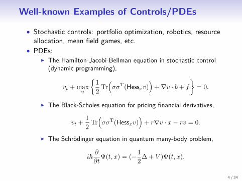
Well-known Examples of Controls/PDEs

• Stochastic controls: portfolio optimization, robotics, resourceallocation, mean field games, etc.

• PDEs:I The Hamilton-Jacobi-Bellman equation in stochastic control

(dynamic programming),

vt + maxu

{12 Tr

(σσT(Hessxv)

)+∇v · b+ f

}= 0.

I The Black-Scholes equation for pricing financial derivatives,

vt + 12 Tr

(σσT(Hessxv)

)+ r∇v · x− rv = 0.

I The Schrodinger equation in quantum many-body problem,

i~∂

∂tΨ(t, x) = (−1

2∆ + V )Ψ(t, x).

4 / 34

Curse of Dimensionality

• The dimension can be easily large in practice.

Equation Dimension (roughly)

HJB equation the same as the state spaceBlack-Scholes equation # of underlying financial assetsSchrodinger equation # of electrons × 3

• A key computational challenge is the curse of dimensionality:the complexity is exponential in dimension d for finitedifference/element method – usually unavailable for d ≥ 4.

• There is a huge gap between stochastic control/PDEmodelings and computational algorithms.

5 / 34

Remarkable Success of Deep Learning

• Machine learning/data analysis also face the same curse ofdimensionality

• In recent years, deep learning has achieved remarkable success

6 / 34

Deep Learning 101

• Representation: in a compositional form rather than additive,

f(x) = Lout ◦ LNh ◦ LNh−1 ◦ · · · ◦ L1(x),

hp = Lp(hp−1) = σ(Wphp−1 + bp

),

σ : element-wise nonlinear activation function: max(0, x),hyperbolic tangent, sigmoid, etc.

• Optimization:

minθ

1N

N∑i=1

L(f(xi; θ)).

Algorithm: stochastic gradient descent (SGD) and its variants.

7 / 34

Table of Contents

1. Background

2. Stochastic Control in Discrete Time

3. BSDE Formulation of Parabolic PDE

4. Neural Network Approximation

5. Numerical Examples

6. Summary

8 / 34

Formulation

Model dynamics:

st+1 = st + bt(st, at) + ξt+1.

State: st, control: at, randomness: ξt. Objective:

min{at}T−1

t=0

E{ T−1∑t=0

ct(st, at(st)) + cT (sT ) | s0},

Define cumulative cost for later use:

Ct =t∑

τ=0cτ (sτ , aτ ), t = 0, 1, · · · , T − 1,

CT = CT−1 + cT (sT ).

9 / 34

Neural Network ApproximationWe look for a feedback control:

at = at(st).

• Traditional methods in operation research: discretize stateand/or control into finite spaces + approximate dynamicprogramming.

• Neural network approximation:

at(st) ≈ at(st|θt),

Solve directly the approximate optimization problem

min{θt}T−1

t=0

E{ T−1∑t=0

ct(st, at(st|θt)) + cT (sT )},

rather than dynamic programming principle.10 / 34

Network Architecture

Figure: Network architecture for solving stochastic control in discretetime. The whole network has (N + 1)T layers in total that involve freeparameters to be optimized simultaneously. Each column (except ξt)corresponds to a sub-network at t.

11 / 34

Table of Contents

1. Background

2. Stochastic Control in Discrete Time

3. BSDE Formulation of Parabolic PDE

4. Neural Network Approximation

5. Numerical Examples

6. Summary

12 / 34

Semilinear Parabolic PDE

We consider a general semilinear parabolic PDE in [0, T ]× Rd:

∂u

∂t(t, x) + 1

2Tr(σσT(t, x)(Hessxu)(t, x)

)+∇u(t, x) · µ(t, x)

+ f(t, x, u(t, x), σT(t, x)∇u(t, x)

)= 0.

• Terminal condition is given: u(T, x) = g(x).

• To fix ideas, we are interested in the solution at t = 0, x = ξfor some vector ξ ∈ Rd.

13 / 34

Connection between PDE and BSDE

• The link between parabolic PDEs and backward stochasticdifferential equations (BSDEs) has been extensivelyinvestigated (Pardoux & Peng 1992, El Karoui et al. 1997,etc).

• In particular, Markovian BSDEs give a nonlinear Feynman-Kacrepresentation of some nonlinear parabolic PDEs.

• Consider the following BSDEXt = ξ +

∫ t

0µ(s,Xs) ds+

∫ t

0σ(s,Xs) dWs,

Yt = g(XT ) +∫ T

tf(s,Xs, Ys, Zs) ds−

∫ T

t(Zs)T dWs,

The solution is an adapted process {(Xt, Yt, Zt)}t∈[0,T ] withvalues in Rd × R× Rd.

14 / 34

Connection between PDE and BSDE• Under suitable regularity assumptions, the BSDE is well-posed

and related to the PDE in the sense that for all t ∈ [0, T ] itholds a.s. that

Yt = u(t,Xt) and Zt = σT(t,Xt)∇u(t,Xt).

• In other words, given the stochastic process satisfying

Xt = ξ +∫ t

0µ(s,Xs) ds+

∫ t

0σ(s,Xs) dWs,

the solution of PDE satisfies the following SDE

u(t,Xt)− u(0, X0)

=−∫ t

0f(s,Xs, u(s,Xs), σT(s,Xs)∇u(s,Xs)

)ds

+∫ t

0[∇u(s,Xs)]T σ(s,Xs) dWs.

15 / 34

BSDE and Control – A LQG ExampleConsider a classical linear-quadratic-Gaussian (LQG) controlproblem in Rd:

dXt = 2√λmt dt+

√2 dWt,

with cost functional J({mt}0≤t≤T ) = E[ ∫ T

0 ‖mt‖22 dt+ g(XT )].

The HJB equation for this problem is

∂u

∂t(t, x) + ∆u(t, x)− λ‖∇u(t, x)‖22 = 0.

The optimal control is given by

m∗t = ∇u(t, x)√2λ

, (recall Zt = σT(t,Xt)∇u(t,Xt)).

In the context of BSDE for control, Yt denotes the optimal valueand Zt denotes the optimal control (up to a constant scaling).

16 / 34

Table of Contents

1. Background

2. Stochastic Control in Discrete Time

3. BSDE Formulation of Parabolic PDE

4. Neural Network Approximation

5. Numerical Examples

6. Summary

17 / 34

Neural Network Approximation

• Key step: approximate the function x 7→ σT(t, x)∇u(t, x) ateach discretized time step t = tn by a feedforward neuralnetwork

σT(tn, Xtn)∇u(tn, Xtn) = (σT∇u)(tn, Xtn)≈ (σT∇u)(tn, Xtn |θn),

where θn denotes neural network parameters.

• Observation: we can stack all the subnetworks together toform a deep neural network (DNN) as a whole, based on thetime discretization (see the next two slides).

18 / 34

Time Discretization

We consider the simple Euler scheme of the BSDE, with apartition of the time interval [0, T ], 0 = t0 < t1 < . . . < tN = T :

Xtn+1 −Xtn ≈ µ(tn, Xtn) ∆tn + σ(tn, Xtn) ∆Wn,

and

u(tn+1, Xtn+1)− u(tn, Xtn)≈− f

(tn, Xtn , u(tn, Xtn), σT(tn, Xtn)∇u(tn, Xtn)

)∆tn

+ [∇u(tn, Xtn)]T σ(tn, Xtn) ∆Wn,

where∆tn = tn+1 − tn, ∆Wn = Wtn+1 −Wtn .

19 / 34

Network Architecture

Figure: Network architecture for solving parabolic PDEs. Each columncorresponds to a subnetwork at time t = tn. The whole network has(H + 1)(N − 1) layers in total that involve free parameters to beoptimized simultaneously.

20 / 34

Optimization

• This network takes the paths {Xtn}0≤n≤N and {Wtn}0≤n≤Nas the input data and gives the final output, denoted byu({Xtn}0≤n≤N , {Wtn}0≤n≤N ), as an approximation tou(tN , XtN ).

• The error in the matching of given terminal condition definesthe expected loss function

l(θ) = E

[∣∣g(XtN )− u({Xtn}0≤n≤N , {Wtn}0≤n≤N

)∣∣2].• The paths can be simulated easily. Therefore the commonly

used SGD algorithm fits this problem well.

• We call the introduced methodology deep BSDE method sincewe use the BSDE and DNN as essential tools.

21 / 34

Table of Contents

1. Background

2. Stochastic Control in Discrete Time

3. BSDE Formulation of Parabolic PDE

4. Neural Network Approximation

5. Numerical Examples

6. Summary

22 / 34

Implementation

• Each subnetwork has 4 layers, with 1 input layer(d-dimensional), 2 hidden layers (both d+ 10-dimensional),and 1 output layer (d-dimensional).

• Choose the rectifier function (ReLU) as the activationfunction and optimize with Adam method.

• Implement in Tensorflow and reported examples are all run ona Macbook Pro.

• Github: https://github.com/frankhan91/DeepBSDE

23 / 34

LQG Example RevisitedWe solve the introduced HJB equation in [0, 1]× R100. It admitsan explicit formula, which allows accuracy test:

u(t, x) = − 1λ

ln(E

[exp

(− λg(x+

√2WT−t)

)]).

0 10 20 30 40 50

lambda

4.0

4.1

4.2

4.3

4.4

4.5

4.6

4.7

u(0,0,...,0)

Deep BSDE Solver

Monte Carlo

Figure: Left: Relative error of the deep BSDE method foru(t=0, x=(0, . . . , 0)) when λ = 1, which achieves 0.17% in a runtime of 330seconds. Right: Optimal cost u(t=0, x=(0, . . . , 0)) against different λ.

24 / 34

Black-Scholes Equation with Default Risk

• The classical Black-Scholes model can and should beaugmented by some important factors in real markets,including defaultable securities, transactions costs,uncertainties in the model parameters, etc.

• Ideally the pricing models should take into account the wholebasket of financial derivative underlyings, resulting inhigh-dimensional nonlinear PDEs.

• To test the deep BSDE method, we study a special case ofthe recursive valuation model with default risk (Duffie et al.1996, Bender et al. 2015).

25 / 34

Black-Scholes Equation with Default Risk

• Consider the fair price of a European claim based on 100underlying assets conditional on no default having occurredyet.

• The underlying asset price moves as a geometric Brownianmotion and the possible default is modeled by the first jumptime of a Poisson process.

• The claim value is modeled by a parabolic PDE with thenonlinear function

f(t, x, u(t, x), σT(t, x)∇u(t, x)

)=− (1− δ)Q(u(t, x))u(t, x)−Ru(t, x).

26 / 34

Black-Scholes Equation with Default RiskThe not explicitly known “exact” solution at t = 0x = (100, . . . , 100) is computed by the multilevel Picard method.

Figure: Approximation of u(t=0, x=(100, . . . , 100)) against number ofiteration steps. The deep BSDE method achieves a relative error of size0.46% in a runtime of 617 seconds.

27 / 34

Allen-Cahn Equation

The Allen-Cahn equation is a reaction-diffusion equation for themodeling of phase separation and transition in physics. Here weconsider a typical Allen-Cahn equation with the “double-wellpotential” in 100-dimensional space:

∂u

∂t(t, x) = ∆u(t, x) + u(t, x)− [u(t, x)]3 ,

with initial condition u(0, x) = g(x).

28 / 34

Allen-Cahn Equation

The not explicitly known “exact” solution at t = 0.3,x = (0, . . . , 0) is computed by the branching diffusion method.

0.00 0.05 0.10 0.15 0.20 0.25 0.30

t

0.00

0.05

0.10

0.15

0.20

0.25

0.30

u(t,0,...,0)

Figure: Left: relative error of the deep BSDE method foru(t=0.3, x=(0, . . . , 0)), which achieves 0.30% in a runtime of 647 seconds.Right: time evolution of u(t, x=(0, . . . , 0)) for t ∈ [0, 0.3], computed by meansof the deep BSDE method.

29 / 34

An Example with Oscillating Explicit Solution

We consider an example studied for the numerical methods of PDEin literature (Gobet & Turkedjiev 2017). We set d = 100 instead ofd = 2.

The PDE is constructed artificially in a form

∂u

∂t(t, x) + 1

2 ∆u(t, x) + min{

1,(u(t, x) − u∗(t, x)

)2} = 0,

in which u∗(t, x) is the explicit oscillating solution

u∗(t, x) = κ+ sin(λ∑di=1 xi

)exp

(λ2d(t−T )2

).

30 / 34

Effect of Number of Hidden Layers

Table: The mean and standard deviation (std.) of the relative error forthe above PDE, obtained by the deep BSDE method with differentnumber of hidden layers.

Number of layers† 29 58 87 116 145

Mean of relative error 2.29% 0.90% 0.60% 0.56% 0.53%Std. of relative error 0.0026 0.0016 0.0017 0.0017 0.0014

† We only count the layers that have free parameters to be optimized.

31 / 34

Effect of Activation Function

Nonlinear BS LQG Allen-CahnReLU 0.46% (0.0008) 0.17% (0.0004) 0.30% (0.0021)Tanh 0.44% (0.0006) 0.17% (0.0005) 0.28% (0.0024)

Sigmoid 0.46% (0.0004) 0.19% (0.0008) 0.38% (0.0026)Softplus 0.45% (0.0007) 0.17% (0.0004) 0.18% (0.0017)

Table: The mean and standard deviation (in parenthesis) of relative errorobtained by the deep BSDE method with different activation functions,for the nonlinear Black-Scholes equation, the Hamilton-Jacobi-Bellmanequation, and the Allen-Cahn equation.

32 / 34

Table of Contents

1. Background

2. Stochastic Control in Discrete Time

3. BSDE Formulation of Parabolic PDE

4. Neural Network Approximation

5. Numerical Examples

6. Summary

33 / 34

Summary

We proposes the so-called deep BSDE method, which can solvegeneral nonlinear high-dimensional parabolic PDEs.

1. We reformulate the parabolic PDEs as BSDEs andapproximate the unknown gradient by deep neural networks.

2. Numerical results validate the proposed algorithm in highdimensions, in terms of both accuracy and speed.

3. This opens up new possibilities in various disciplines involvingPDE modelings.

Thank you for your attention!

34 / 34