Deep Convolutional Neural Network for Effective Image Analysis

DESIGN AND IMPLEMENTATION OF A DEEP PIXEL-WISE SEGMENTATION ARCHITECTURE MARC ROS MARTÍ

KTH ROYAL INSTITUTE OF TECHNOLOGY

I N F O R M A T IO N A N D C O M M U N I C A T I O N T E C H N O L O G Y

Abstract

This master thesis presents the process of designing and implementing a CNN-based architecture for image recognition included in a larger project in the field of fashion recommendation with deep learning. Concretely, the presented network aims to perform localization and segmentation tasks. Therefore, an accurate analysis of the most well-known localization and segmentation networks in the state of the art has been performed. Afterwards, a multi-task network performing RoI pixel-wise segmentation has been created. This proposal solves the detected weaknesses of the pre-existing networks in the field of application, i.e. fashion recommendation. These weaknesses are basically related with the lack of a fine-grained quality of the segmentation and problems with computational efficiency. When it comes to improve the details of the segmentation, this network proposes to work pixel-wise, i.e. performing a classification task for each of the pixels of the image. Thus, the network is more suitable to detect all the details presented in the analysed images. However, a pixel-wise task requires working in pixel resolution, which implies that the number of operations to perform is usually large. To reduce the total number of operations to perform in the network and increase the computational efficiency, this pixel-wise segmentation is only done in the meaningful regions of the image (Regions of Interest), which are also computed in the network (RoI masks). Then, after a study of the more recent deep learning libraries, the network has been successfully implemented. Finally, to prove the correct operation of the design, a set of experiments have been satisfactorily conducted. In this sense, it must be noted that the evaluation of the results obtained during testing phase with respect to the most well-known architectures is out of the scope of this thesis as the experimental conditions, especially in terms of dataset, have not been suitable for doing so. Nevertheless, the proposed network is totally prepared to perform this evaluation in the future, when the required experimental conditions are available. Keywords: CNN, Co-CNN, segmentation, localization, RoI, masking, RoI masking, multi-task network, pixel resolution, overfitting

Abstract

Denna examensarbete presenterar processen för att designa och implementera en CNN-baserad arkitektur för bildigenkänning som ingår i ett större projekt inom moderekommendation med djup inlärning. Konkret, det presenterade nätverket syftar till att utföra lokaliserings- och segmenteringsuppgifter. Därför har en noggrann analys av de mest kända lokaliserings- och segmenteringsnätena utförts inom den senaste tekniken. Därefter har ett multi-task-nätverk som utför RoI pixel-wise segmentering skapats. Detta förslag löser de upptäckta svagheterna hos de befintliga näten inom tillämpningsområdet, dvs modeanbefaling. Dessa svagheter är i grund och botten relaterade till bristen på en finkornad kvalitet på segmenteringen och problem med beräkningseffektivitet. När det gäller att förbättra detaljerna i segmenteringen, föreslår detta nätverk att arbeta pixelvis, dvs att utföra en klassificeringsuppgift för var och en av bildpunkterna i bilden. Nätverket är sålunda lämpligare att detektera alla detaljer som presenteras i de analyserade bilderna. En pixelvis uppgift kräver dock att man arbetar med pixelupplösning, vilket innebär att antalet operationer som ska utföras är vanligtvis stor. För att minska det totala antalet operationer som ska utföras i nätverket och öka beräkningseffektiviteten görs denna pixelvisa segmentering endast i de meningsfulla regionerna i bilden (intressanta regioner), som också beräknas i nätverket (RoI-masker) . Sedan, efter en studie av de senaste djuplärningsbiblioteken, har nätverket framgångsrikt implementerats. Slutligen, för att bevisa korrekt funktion av konstruktionen, har en uppsättning experiment genomförts på ett tillfredsställande sätt. I detta avseende måste det noteras att utvärderingen av de resultat som uppnåtts under testfasen i förhållande till de mest kända arkitekturerna ligger utanför denna avhandling, eftersom de experimentella förhållandena, särskilt vad gäller dataset, inte har varit lämpliga För att göra det. Ändå är det föreslagna nätverket helt beredd att utföra denna utvärdering i framtiden när de nödvändiga försöksvillkoren är tillgängliga. Nyckelord: CNN, Co-CNN, segmentering, lokalisering, RoI, maskering, RoI-maskering, flera uppgiftsnätverk, pixelupplösning, övermontering

Resum En aquest treball de fi de màster es presenta el disseny i la implementació d’una arquitectura pel reconeixement d’imatges fent ús de CNN. Aquesta xarxa es troba inclosa en un projecte de major envergadura en el camp de la recomanació de moda. En concret, la xarxa presentada en aquest document s’encarrega de realitzar les tasques de localització i segmentació. Després d’un estudi a consciència de les xarxes més conegudes de l’estat de l’art, s’ha dissenyat una xarxa multi-tasca encarregada de realitzar una segmentació a resolució de píxel de les regions d’interès de la imatge, les quals han sigut prèviament calculades i emmascarades. Aquesta proposta soluciona les mancances detectades en les xarxes ja existents pel que fa a la tasca de recomanació de moda. Aquestes mancances es basen en la obtenció d’una segmentació sense prou nivell de detalls i en una rellevant complexitat computacional. Pel que fa a la qualitat de la segmentació, aquesta tesi proposa treballar en resolució de píxel, classificant tots els píxels de la imatge de forma individual, per tal de poder adaptar-se a tots els detalls que puguin aparèixer a la imatge analitzada. No obstant, treballar píxel a píxel implica la realització d’una gran quantitat d’operacions. Per reduir-les, proposem fer la segmentació píxel a píxel només a les regions d’interès de la imatge. A continuació, després d’un estudi detallat de les llibreries de deep learnign més destacades, el disseny ha sigut implementat. Finalment s’han dut a terme una sèrie d’experiments per provar el correcte funcionament del disseny. En aquest sentit és important destacar que aquesta tesi no té com a objectiu avaluar el disseny respecte d’altres xarxes ja existents. La raó és que les condicions d’experimentació, sobretot pel que fa a la base de dades, no són adequades per aquesta tasca. No obstant, la xarxa està perfectament preparada per fer aquesta avaluació un cop les condicions d’experimentació així ho permetin. Paraules clau: CNN, segmentació, localització, RoI, emmascarar, filtratge de RoIs, xarxa multi-tasca, resolució de píxel, overfitting

Acknowledgements

First of all, I would like to thank my supervisor Shatha Jaradat for presenting me the possibility of doing an attractive Deep Learning project in KTH and for helping me during my whole stay in Sweden. It has been an honor to work with her and learn about her professional methodology and experience. I would also like to show my gratitude for her honesty and for treating me like a little brother, with some advices that will make me grow up and I will always remember. Thanks a lot, Shatha! Also, I would like to thank Prof. Mihhail Matskin for his excellent personal treatment, for believing in my capabilities and for providing the working conditions of the thesis. Thanks also to Enric Monte for being the co-director of my thesis in UPC. Finalment m’agradaria agrair a la meva família i amics tot el suport que m’han donat durant tots aquests anys de carrera que aquí finalitzen. No voldria personalitzar, però aquesta aventura seria difícil d’entendre sense el Lucas. Moltes gràcies amic, per donar-me l’empenta necessària per anar a Suècia i per fer-me la vida més fàcil allà: Deep learning, plats bruts i dards. I per últim, unes paraules especials per la Laura: separar-me de tu va ser la part més difícil de començar aquesta aventura però sempre agrairé com vas saber fer-te tan propera malgrat la distància. Gràcies per la teva generositat, per ser la primera persona amb qui puc parlar quan tinc un mal dia i per la teva paciència i comprensió durant les moltes hores de més que he hagut de dedicar a aquesta tesis en comptes de a tu. T’estimo. En resum, ja sabeu, això va pels de sempre i la Laura.

Table of Contents

1 Introduction ............................................................................................................. 1 1.1 Background .................................................................................................................. 1 1.2 Problem .......................................................................................................................... 1 1.3 Purpose ........................................................................................................................... 2 1.4 Goal ................................................................................................................................... 2

1.4.1 Benefits, Ethics and Sustainability ............................................................................... 2 1.5 Methodology / Methods ......................................................................................... 2 1.6 Delimitations ............................................................................................................... 3 1.7 Outline (Disposition) .............................................................................................. 3

2 Theoretic Background: Transition to Deep Learning ...................... 5 2.1 Convolutional Neural Networks (CNN) ....................................................... 5

2.1.1 CNN Architecture: Main Operations ........................................................................... 6 2.1.1.1 Input .............................................................................................................................................7 2.1.1.2 Convolutional Layer...........................................................................................................7 2.1.1.3 Activation Function ......................................................................................................... 10 2.1.1.4 Pooling Layer ...................................................................................................................... 12 2.1.1.5 Fully Connected Layers ................................................................................................. 13

2.2 Image Recognition: Image detection and localization ...................... 13 2.2.1.1 Object Proposal .................................................................................................................. 14 2.2.1.2 Bounding-Box Regression ........................................................................................... 14

2.3 Image Recognition: Segmentation ................................................................ 14 2.3.1.1 Over-Segmentation .......................................................................................................... 15

3 Study and analysis of the related work .................................................. 16 3.1 CNN for Localization ............................................................................................. 16

3.1.1 R-CNN ......................................................................................................................................16 3.1.2 SPPnet ......................................................................................................................................17

3.1.2.1 SPP layer ................................................................................................................................ 18 3.1.3 Fast R-CNN ............................................................................................................................18

3.1.3.1 RoI Pooling Layer ............................................................................................................. 20 3.1.4 Faster R-CNN ........................................................................................................................20

3.1.4.1 RPN ............................................................................................................................................ 21 3.2 CNN for Segmentation ......................................................................................... 22

3.2.1 FCN ............................................................................................................................................22 3.2.1.1 Fractional-Stride Convolution .................................................................................. 24

3.2.2 Hypercolumns for Segmentation ................................................................................24 3.2.3 MNC for Segmentation ....................................................................................................27

3.2.3.1 Stage 1: Regressing Box-Level instances ........................................................... 29 3.2.3.2 Stage 2: Regressing Mask-Level instances ....................................................... 29 3.2.3.3 Stage 3: Categorizing instances .............................................................................. 29

3.2.4 Human Parsing with Contextualized CNN for Segmentation .......................30 3.2.4.1 Cross-Layer Context: Local-to-global-to-local hierarchy ...................... 31 3.2.4.2 Global Image-Level Context ....................................................................................... 32 3.2.4.3 Local Super-Pixel Context ............................................................................................ 33

4 Architecture Design .......................................................................................... 35 4.1 Image Recognition Network ............................................................................. 36

4.1.1 Pre-processing module .....................................................................................................37 4.1.1.1 Mask creation: Faster R-CNN masking (RoI masking) ........................... 37

4.1.2 Pixel-wise Segmentation .................................................................................................38 4.1.2.1 Cross-Layer Context ........................................................................................................ 40 4.1.2.2 From Global Image-Level Context to Global RoI-Level Context ......... 40 4.1.2.3 Suppression of the Local Super-Pixel Context................................................. 41

4.1.3 Shared Convolutional Module ......................................................................................42 4.1.4 Integration between modules .......................................................................................42

4.2 Integration with the rest of the architecture .......................................... 42 4.2.1 Integration with image retrieval ..................................................................................43

4.2.1.1 Image retrieval: a one-to-many process ........................................................... 43 4.2.1.2 Integration with the Segmentation task ............................................................. 44

4.2.2 Integration with Text Processing ................................................................................44 4.3 RoI pixel segmentation vs. existing architectures ............................... 44

4.3.1 Comparison with MNC .....................................................................................................45 4.3.2 Comparison with Human Parsing ..............................................................................45

5 Implementation ................................................................................................... 47 5.1 Training Input: PASCAL VOC 2012 Dataset ............................................ 47

5.1.1 Ground Truth Mapping ....................................................................................................48 5.1.2 Problems with the dataset: lack of some box annotations ..............................48

5.2 Architecture Implementation .......................................................................... 49 5.2.1 Shared Convolutional Layers ........................................................................................49 5.2.2 Pixel-wise Segmentation Module ................................................................................52

5.2.2.1 Prediction processing ..................................................................................................... 54 5.3 Size incompatibility during Upsampling .................................................. 55

5.3.1 Upsampling incompatibility example .......................................................................55 5.3.2 Solving Upsampling incompatibility: Crop Layer ...............................................56

5.4 Learning configuration: multi-task single-stage learning .............. 57 5.4.1.1 Ground Truth Masking ................................................................................................. 59

5.5 Visualization of the prediction process ..................................................... 60 5.5.1 Prediction processing: correcting the Background score ................................63 5.5.2 Ground Truth Masking visualization ........................................................................63

5.6 Server selection ........................................................................................................ 66

6 Results ....................................................................................................................... 67 6.1 Evaluation metrics ................................................................................................. 67 6.2 Testing conditions .................................................................................................. 67

6.2.1 Definition of the learning parameters.......................................................................68 6.3 Numerical results ................................................................................................... 68

6.3.1 Analysis of the results .......................................................................................................69 6.3.1.1 Responsibility of the dataset in the results: overfitting ............................ 69 6.3.1.2 Responsibility of the server in the results .......................................................... 71 6.3.1.3 Responsibility of the design in the results ......................................................... 72

7 Conclusions and future work....................................................................... 74

References ....................................................................................................................... 75

Appendix A ......................................................................................................................... 1

Appendix B ......................................................................................................................... 1

1

List of figures

Figure 1: Example of a CNN architecture for object classification .................... 6

Figure 2: Process of applying a filter and moving it in the whole image ........... 7

Figure 3: Illustration of stride difference ........................................................... 9

Figure 4: Example matrix with padding............................................................. 9

Figure 5: Resulting matrix after applying the filter on the input image ......... 10

Figure 6: Activation functions ........................................................................... 11

Figure 7: ReLU activation function ................................................................... 11

Figure 8: Max-pooling example ........................................................................ 12

Figure 9: Classification vs. localization vs. detection vs. segmentation ........... 13

Figure 10: Segmentation example ..................................................................... 15

Figure 11: Summary of the operation of R-CNN ............................................... 17

Figure 12: Fast R-CNN architecture .................................................................. 19

Figure 13: Faster R-CNN modules ................................................................... 22

Figure 14: FCN architecture ............................................................................. 23

Figure 15: Segmentation of an image by means of Hypercolumns .................. 27

Figure 16: Multi Task Network vs. Multi-Task Network Cascade ................... 27

Figure 17: MNC Architecture for an instance-aware semantic segmentation. 28

Figure 18: Human Parsing with Co-CNN for Segmentation Architecture ....... 31

Figure 19: MNC vs. Human Parsing ................................................................. 35

Figure 20: Proposed RoI pixel-wise segmentation network ............................ 36

Figure 21: Pre-processing module of the proposed network ........................... 38

Figure 22: Segmentation module of the proposed network ............................ 39

2

Figure 23: RGB ground truth label example .................................................... 47

Figure 24: Grayscale ground truth label example ............................................ 48

Figure 25: Training configuration. ................................................................... 57

Figure 26: Visualization process: feature map ................................................. 60

Figure 27: Visualization process: ground truth mapping ................................ 60

Figure 28: Visualization process: prediction maps ........................................... 61

Figure 29: Visualization process: position evaluation I ................................... 62

Figure 30: Visualization process: position evaluation II ................................. 62

Figure 31: Visualization process: correcting the background .......................... 63

Figure 32: Visualization process: incorrect mask generation .......................... 64

Figure 33: Visualization process: prediction with incorrect mask and

background not corrected ................................................................................. 64

Figure 34: Visualization process: prediction with incorrect mask with

background correction ...................................................................................... 64

Figure 35: Visualization process: evaluation with incorrect mask with

background correction ...................................................................................... 65

Figure 36: Visualization process: ground truth masked .................................. 65

Figure 37: Visualization process: evaluation with ground truth masked ........ 66

3

List of tables

Table 1: Architecture Overview......................................................................... 49

Table 2: VGG architectures ............................................................................... 50

Table 3: AlexNet Configuration ......................................................................... 51

Table 4: Pixel-wise Segmentation Module Configuration ............................... 53

Table 5: Results of the proposed network ........................................................ 68

Table 6: Human Parsing Results ...................................................................... 69

Table 7: Results: Our network vs. Human Parsing .......................................... 70

1

1 Introduction

Artificial Intelligence (AI) is revolutionizing how science is done. The point is that these systems, referred as neural networks, with a minimal amount of human contribution are progressively learning how to learn on their own: from large training datasets, they can find patterns to be applied for several tasks [1]. Among these tasks, image recognition is one of the most challenging and interesting to develop. In image recognition, tasks as varied as classification, localization, detection or segmentation are applied in a wide range of fields: from medical applications to the fashion industry. The work presented in this thesis aims to present the design, implementation and a preliminary evaluation of an image recognition network using deep learning [2]. This thesis is part of the PhD work done by Shatha Jaradat in the field of fashion recommendation. Concretely, the presented architecture performs the image recognition tasks of the network presented in [3], paper that summarizes the project of Shatha in fashion recommendation.

1.1 Background

To fulfill the requirements of the work presented in [3], the deep learning network created in this thesis has to be able to perform both a localization and segmentation task. Localization consists in locating where in the image an object is set and segmentation consists in detect and classify the regions that form the analysed image. In that regard, papers of how these techniques are performed using both deep and non-deep learning algorithms have been studied. This thesis includes a summary of the deep algorithms used to perform these tasks (see section 4). Convolutional Neural Networks (CNN) [4] are the typical image recognition networks applied when using deep learning. Consequently, in the design presented in this thesis, CNNs are implemented. Details about the implementation and operation of CNNs are presented in section 2. To understand the operation of CNNs and its implementation using deep learning libraries, the author of this thesis has followed the Stanford University course in CNN [5] and several deep learning libraries tutorials in Tensorflow [6] and Keras [7].

1.2 Problem

The architecture presented in [3] is a challenging and ambitious network that requires a powerful image recognition module able to perform a segmentation task in the most possible optimized way considering the integration of this module with the rest of the architecture. This thesis presents both the design and the implementation of said image recognition network. Consequently, this

2

work aims to give answer to two different points: which is the best way to design an image recognition network suitable for [3] and, once it is implemented, evaluate if the quality of the results is as good as expected.

1.3 Purpose

This master thesis presents the most relevant part of the work performed during the realization of the project: it starts with an accurate analysis of the techniques and papers related with the subject of study, continues with an illustration of the network design and an explanation of its more relevant components, shows how the implementation of the design has been carried out and finally discusses the results obtained when testing on the resulting architecture.

1.4 Goal

The main objective of this master thesis is to perform an accurate analysis of the state of the art of the current deep learning algorithms for image recognition (e.g. localization, detection and segmentation) so as to come up with a new architecture design that fulfills the requirements to be integrated in [3] better than the pre-existing options of the state of the art. Furthermore, once the design is completed, the network has to be implemented and tested. Nevertheless, it is not an objective of this thesis neither to evaluate it nor compare with the most well-known architectures in the state-of-the-art, as the available resources do not allow to perform an accurate evaluation.

1.4.1 Benefits, Ethics and Sustainability

AI is going to be applied continuously in the everyday life of an average person. In the case of image recognition, a network like the one presented in this thesis is going to be suitable, just to give some examples, for medical applications (e.g. looking for some patterns that might reveal a disease in an x-ray image), surveillance (e.g. detecting from images the person that matches a certain description) or, like in [3], fashion recommendation. Nevertheless, as AI works with huge amount of data, it is going to certainly expose information from a great amount of people. Therefore, it is necessary to ensure that their privacy is always preserved.

1.5 Methodology / Methods

Both qualitative and quantitative research methodologies have been applied in this project. This corresponds to the fact that this work has consisted in two main tasks: network design and network implementation. In terms of network design, a qualitative research method has been applied: there is a lot of

3

literature to review so as to understand the methodologies applied depending on the task. On the other hand, in terms of network implementation, a quantitative methodology focus on obtaining results is performed. The phases of the project can be described in the following steps:

- Detailed literature study about deep learning, focusing specially on how CNNs work.

- Read and study of papers related with the field of research: localization and segmentation using deep and non-deep learning algorithms.

- Taking ideas from the previous background, design an image recognition network ready to be integrated in the architecture presented in [3].

- Learn how to work in a deep learning programming environment: Python and deep-learning libraries.

- Conscious study of the implementation in code of the already existing architectures which are used in our new image recognition network.

- Dataset and server selection according to the available resources. - Implementation of the design. - Experimentation to prove the correct implementation of the network.

1.6 Delimitations

The most important delimitations of this work have been due to the time and some resources limitations. Concerning the time, it is a clear limiting factor taking into account that the objective is the creation, from scratch, of an image recognition networks that ideally should be prepared to give good results. On the other hand, in terms of resources, to ensure that a deep learning algorithm works correctly, a large dataset is indispensable. This requirement highlights the necessity of having a powerful server able to handle the large amount of data available in the dataset. Unfortunately, a large dataset suitable for the task was not available within the time of this thesis and there were limitations in the selected server’s capabilities. In the case of the dataset, a large and suitable dataset is being gathered in another master thesis performed in parallel with this one. However, it has suffered from an important delay and has not been possible to use it for this work. Finally, regarding the server, after dealing with a lot of issues, the selected one has not fulfilled the capacity expectations. Thus, as the resources have not been optimal, it is not performed an evaluation of the worthiness of the design based on the results obtained in the test phase.

1.7 Outline (Disposition)

This report is organized as follows. Section 2 provides a background study focused on CNNs and the image recognition tasks to be performed in the network: localization and segmentation. Section 3 includes a summary of the most important papers and techniques from the state of the art that have been

4

studied to come up with a new design. Section 4 presents the details related with the design of the network, explains its integration in [3] and compares it to the networks of the state of the art. Section 5 includes the implementation details of the network. Section 6 presents the evaluation of the architecture after testing phase and, finally, section 7 gives the conclusion and expected feature work.

5

2 Theoretic Background: Transition to Deep Learning

This master thesis presents the design of the image recognition architecture of the proposal made in [3]. In it, fashion images are analysed in order to perform a recommendation task, e.g. brand/style recommendation. Consequently, an important analysis of the techniques and possibilities in the image recognition field has been carried out, focusing specifically in the methods offered by the traditional computer vision models and the ones where deep learning is applied. When it comes to analysing the content of an image, the traditional computer vision and image processing algorithms have provided pioneering solutions with excellent results. Tasks such as object detection, localization and segmentation have been widely used for a great amount of purposes, covering a wide range of applications: from surveillance and biometrics to videogames and leisure activities. Recently, the application of deep learning for computer vision tasks has changed the scenario: while in traditional computer vision methods feature extraction is required as a pre-processing step before feeding the non-deep machine learning or equivalent decision algorithm, no pre-processing has to be done in deep learning, as the features are extracted inside the network. This is a relevant change because the feature extraction process is not learnable in the traditional machine learning architectures for computer vision and even less in an image processing technique where any machine learning algorithm is applied [8]. On the other hand, the utilization of deep learning for these tasks allow them to be trainable end-to-end, i.e. to learn also how to perform the feature extraction. In this work, the image recognition network is going to be implemented using deep learning techniques; concretely, Convolutional Neural Networks (CNN) [4]. It has been selected instead of the traditional machine learning algorithms for computer vision because of the arguments of the previous paragraph: the possibility of performing an end-to-end training without pre-processing steps. In the following sections, an introduction of how CNN work and a summary of the image processing techniques that have been considered for these task, i.e. object detection, localization and segmentation, are going to be presented.

2.1 Convolutional Neural Networks (CNN)

Convolutional Neural Networks (CNN or ConvNets) are a specific type of artificial neural networks that have revolutionized object and speech recognition [4][8]. They are designed to use minimal amounts of pre-processing and have a wide application in image and video recognition, and natural language processing. CNNs were inspired by the organization of animals’ visual cortex, which has small regions of cells (known as receptive fields) that are sensitive to specific regions of the visual field. In an experiment

6

made by Hubel and Wiesel in 1962 [9], they showed that some individual neuronal cells in the brain responded or fired only in the presence of edges of a certain orientation, and others respond to other types of stimuli. They found that all these neurons were organized in a hierarchical architecture and that together, they were able to produce visual perception. In the same way, the low-level features (such as edges and curves) are identified in the first layers of CNNs, then building up to more abstract concepts through a series of layers. The name of these networks (convolutional) is related to the fact that the response of a neuron to a stimulus within its receptive field can be approximated by the mathematical convolution operation [10].

Figure 1: Example of a CNN architecture for object classification. Source: [11]

A simplified description of the mechanism that CNN uses in the first CONV layer is given as follows: given an input image as the one in Figure 1, it is analysed region by region. It is done with different filters that are applied to small windows (receptive field) of the image. Then, the whole image is analysed by moving the filter along all the positions; operating in each location with all the values inside the filter dimensions, i.e. the receptive field. Depending on the values of the filters they are going to be more suitable for extracting different type of features. For example, they can be adapted to the shape of a curve with a certain orientation. We can think of it as a search operation, we look where in the image there is this curve for example. Each filter will result in one of the activation maps. So, in the first CONV layer, we can get many activation maps resulting from straight edges, curves and other types of filters. Applying convolution in multiple layers, will result in identifying the high-level features of the object in a hierarchical style. At the end, it is going to be able to classify the objects in the image.

2.1.1 CNN Architecture: Main Operations

CNNs are built up with a basic structure based on the combination of four different types of layers, as presented in the following scheme:

Input [ [CONV ReLU] * N POOL] * M [FC ReLU] * K FC

7

Where N, M and K are integer values typically between 1 and 3 [8]. These values are set depending on the needs of the network, allowing the creation of deeper networks for those tasks where a more complex structure is required. On the other hand, Input, CONV, ReLU [18], POOL and FC are the different type of layers and important elements that appear in a typical CNN architecture. All of them, together with its main operations, are going to be presented in the following sections.

2.1.1.1 Input

CNNs take images as input. Images are represented by an array of pixel values with three dimensions (height, width, and the RGB values (colour channels)). For example, an image with height = 480, width = 480 will be presented as a 480 × 480 × 3 tensor. Each of the points in the image take a value between 0 and 255 which describes the pixel intensity at that position.

2.1.1.2 Convolutional Layer

Also known as CONV layers, this type of layer is always the first layer in a CNN. In CONV layers, filters (kernels) that stride across all the areas in the input image are applied. The area that the filter covers is the receptive field. The dimensions of the filter are height ×width × depth. Where the depth is the same as the input of the layer. As the filter strides (convolves) over the input image, it multiplies (element-wise multiplication) the values in the filter with the original pixel values of the image. This process is repeated for every location in the input volume. The filter is moved by a certain number of units, which is defined by the stride parameter. The result is a feature or activation map. The more filters, the greater depth of the activation map, and the more information about the input image. Figure 2: A visualisation of the process of applying a filter and moving it in the whole image.

Source: [12]

As mentioned before, the low-level features are usually detected in the first layers, but in order to detect whether the image is a type of object, the network needs to recognize higher-level features. This is achieved by providing the output (activation maps) of a certain layer as an input to another

8

convolutional layer. Thus, the input will be a description of the locations in the original image for where certain low-level features appear. By applying a set of filters on top of that, the output will be activations that represent higher-level features. As we go deeper in the network, we get activation maps that represent more and more complex features. As the network deepens, the filters start having larger effective receptive fields. This does not mean that the actual receptive field is increased, strictly the receptive field could be the same. The difference is that, due to the downsampling experienced in a CNN (explained later in this section), with the same values, they span the equivalent of larger regions of the original input (the image). This is essential in classification tasks as the analysis of larger regions of the input allow to obtain the required global information. The network learns how to adjust its filter values or weights through optimization algorithms, typically using Stochastic Gradient Descent (SGD) [13] with backpropagation [14]. The training process has four main steps: forward pass, loss function, backward pass and weight update. At the beginning, the filter values are randomized. During forward pass, we take an input image and pass it through the whole network. Since all the weights (filter values) are randomized in the first round, the output will not give any relevant preference to any particular class (in image classification tasks for example). The objective after computing the loss function is to get the weights adjusted to minimize the loss. To achieve this, we take the derivative of the loss with respect to the weights. The backward pass is done through the network, which helps in determining which weights contributed the most to the loss and finding ways to adjust them and decrease the loss. The weights get updated so that they change in the negative direction of the gradient according to a learning rate. The learning rate is a hyperparameter chosen by the programmer which remains fixed when using SGD [13]. Higher learning rate means bigger steps taken for weight updates and thus it may take less time for the model to converge on an optimal set of weights. However, high learning rates could result in non-precise and too large jumps, being even unable to reach the minimum. On the other hand, smaller learning rates ensure not to go by the minimum but need a lot of time to converge. Usually it is better to set higher values in the beginning of training when the optimum is still far and decreasing it when the network is more tuned. This highlights the need of using dynamic learning rates instead of fixing them, like in SGD [13]. This is the reason why there are methods that compute them dynamically such as Adagrad, RMSprop or Adam [15][16]. The process of training is repeated for a fixed number of epochs. Once the parameter updates are finished, the network should be trained well enough so that the weights of the layers are turned correctly. With more training data for the network, the more training iterations we can have, and the more weight updates and better network tuning. The parameters that change the behaviour in CONV layers are the stride and padding. The stride controls the amount by which the filter shifts. For example, if the stride is 1, the filter convolves around the input volume by

9

shifting one unit at a time. It should be set in a way that ensures that the output is an integer not a fraction. In Figure 3, the difference between applying a 3 × 3 filter with stride = 1 and stride = 2 is shown, demonstrating that if the stride increases the output dimensions shrink.

Figure 3: Illustration of the difference between applying a 3 × 3 filter with stride = 1 and stride = 2. Source: [12]

As we keep applying CONV layers, the size of the output decreases faster. However, the dimensionality reduction is performed exclusively in the edge values of the feature map. This happens because to apply a convolution, the entire receptive field of the filter must fit inside the map, which is not possible for the positions in the edge. Consequently, it is preferable to force the output to maintain the size of the input. The available tool to ensure that the dimensions are kept is padding. It consists in applying a set of zero values around the feature map as shown in Figure 4:

Figure 4: The resulted matrix after applying zero padding of 2 to a 32×32×3. Source: [12]

10

The way of selecting the padding to maintain the input dimensions depends on the receptive field of the applied filters. Assuming a stride = 1, the formula for the padding that prevent the dimensions from being reduced is the following:

Zero padding = (𝐹−1)

2

Where F is the receptive field (spatial dimensions) of the filters applied. In general terms, the formula for calculating the output size for any CONV layer is as follows:

O = (𝐼 − 𝐹 + 2𝑃)

𝑆 + 1

Where O is the output height/length, I is the input height/length, F is the filter size (receptive field), P is the padding and S is the stride [8]. For example, in the figure below, the result of applying a 5 ×5 ×3 (F=5) filter with stride = 1 (S=1) and without padding (P=0) on a 32 × 32 × 3 (I=0) is visualized in the second part of the figure, which has the dimensions 28 × 28 × 1 (O=0). As it can be seen the absence of padding provokes a reduction of dimensionality. The depth of the output (output channels) depends on the number of filters applied. For example, if two filters were applied, the activation maps would be 28 × 28 × 2.

Figure 5: The matrix that results after applying the filter on the input image Source: [17]

2.1.1.3 Activation Function

It is a convention to apply a non-linear layer (activation layer) after CONV layers, to introduce a non-linearity in the network. There are several reasons to introduce these non-linearities. On the one hand, they are a good way to simulate the biological functionality of a neuron: when the input impulse is strong enough, the neuron activates; otherwise, it does not do anything [4][8]. Moreover, non-linearities are necessary for analysing non-linear patterns. In

11

fact, the operations performed in a neural network are basically linear (dot products), reason why they are suitable for linear patterns. On the contrary, its linearity complicates the analysis of non-linear functions. Activation functions introduce a non-linear behaviour to the network, making also possible the analysis of non-linear patterns. In the origins of CNNs, non-linear functions such as tanh, sigmoid were used but researchers found that ReLU (Rectified Linear Unit) [18] layers work better because the network is able to train faster without making a significant difference to the accuracy. They also help in avoiding the vanishing gradient problem. The vanishing gradient problem occurs in sigmoid and tanh units, where the gradient essentially becomes zero after a certain amount of training and it stops all learning in that section of the network. As shown in Figure 6, it happens because sigmoid and tanh saturate in 1. This provokes that, in saturation zones, the gradient for the activations is almost 0, making the learning process very slow or, eventually, terminating it.

Figure 6: (a) Sigmoid activation function. (b) tanh activation function. Source: [19]

Applying ReLU [18], function f(x) = max(0, x), avoids said problem. As shown in Figure 7, no saturation occurs in the positive domain. Nevertheless, note that all the presented activation functions saturate in the negative domain. This is not a problem; this part is reserved for those values which should not be activated. Therefore, it is convenient that no learning process starts from these values, as they do not fulfil the criteria to be considered in the process.

Figure 7: ReLU activation function. Source: [19]

12

2.1.1.4 Pooling Layer

As previously described in section 2.1.1.2 (padding), maintaining the input dimensions when performing the convolution was appropriated to retain the information present in the edges (otherwise lost). Nevertheless, after some CONV - ReLU layers, downsampling should be applied. As stated, CNNs have images as inputs. The reason is that if FC layers were used, the number of operations to perform would be huge, as the input values in an image are very big (in part due to the three dimensionalities of RGB channels). When going through pooling layers, the dimensionality of the input is reduced, making it more suitable for the final FC layers of the CNN as less operations are required. Among the different options for pooling, i.e. average pooling, L2-norm pooling and max pooling, the most popular one is max pooling [8]. Like in Convolutional Layers, max pooling analyses the input by regions, determined by the receptive field and stride parameters. The difference is that, instead of filtering the input, it takes the maximum values for each of the analysed sub-regions. This region analysis allows not only to perform a dimensionality reduction but also to ensure that the obtained values have local-information awareness, which is especially important for image recognition. This happens because, when taking the maximum value of a concrete region, it is ensured that the dimensionality reduced output consists of local representative values of the original input. Figure 8 presents an example of applying max pooling with a 2 × 2 filter and stride of 2.

Figure 8: Example of applying max pooling with a 2× 2 filter and stride of 2. Source: [12]

Finally, the mathematical expression that relates the dimensionality reduction with the selected receptive field and strive parameters is the following:

O = (𝐼 − 𝐹 )

𝑆 + 1

Where I and O refer to the input and output dimension, respectively; F, to the receptive field (kernel size) and S to the stride [8].

13

2.1.1.5 Fully Connected Layers

Fully connected layers (FC layers) are added at the end of the network, where they take as input the output of a CONV/ReLU/Pool previous layer. The objective of this type of layers in image classification tasks is to determine the features that correlate the most to a particular class, and produces an N dimensional vector where N is the number of classes that the program has to choose from. For example, if the program is predicting that some image represents a person, then it will have high values in the activation maps that represent high level features like hands, face, arms, etc. Examples of classifiers that can be used in final layers is the Softmax function [20] which performs logistic regression to regularize outputs to values between zero and one.

2.2 Image Recognition: Image detection and localization

The detection and localization of the elements that appear in an image has been always a useful and challenging technique in image processing. Computer vision techniques as the SIFT feature descriptor [21] have been widely used to perform these tasks. In a way that stands out for its simplification: detecting an object can be as easy as matching it with a SIFT reference [21]. Figure 9 illustrates the differences between object classification, detection, localization and segmentation.

Figure 9: (a) Object classification - the task of classifying that the picture is a dog. (b) Object localization - decides the bounding box of where the object is located. (c) Object detection - involves the localization of multiple objects that don’t have to be from the same class. (e) Object segmentation - decides the class label and decides an outline of the object. Source: [22]

Localization and detection are referred usually equivalently. In principle, in localization only one instance is located, but in practical terms it can be also used in the case where more than one element is located in the image.

14

Concretely, it is a process where a single object bounding box should be predicted for each of the instances in the image. The basic concepts that are needed to perform localization are described in the subsections below. More details about localization using deep learning methods are provided in section 3.

2.2.1.1 Object Proposal

Object proposals are regions of an image that are supposed to contain an object. Nevertheless, they are not an accurate region. These proposals are typically refined by localization methods (section 3.1). Sometimes they are also referred as RoIs, Region Proposals, Bounding-Box or simply boxes [23]. Each of them is described using 4 real-valued numbers:

1) X coordinate from the centre of the box. 2) Y coordinate from the centre of the box. 3) Width of the box. 4) Height of the box.

2.2.1.2 Bounding-Box Regression

Bounding-box regression is the process that aims to improve the accuracy of an Object Proposal. As its name indicates, it modifies the bounds of a box (characterized using centre, width and height) so as to adjust it to its ideal version, i.e. ground truth box. Inside the architecture of a CNN, bounding-box Regression is, in terms of localization, the equivalent learning process that takes place for classification, i.e. after introducing an input to the network, the given results are improved by fine-tuning the weights that describe said network according to a loss function focused in the concrete task (in this case, reducing the difference between the proposed box and the ground-truth box) [23].

2.3 Image Recognition: Segmentation

Segmentation consists in taking an image and split it in a set of labelled regions. The number of regions could be either selected by the user or automatically generated. Segmentation is sometimes referred as a pixel classification and this is what differentiates if from localization and object detection tasks: it is more precise. In effect, all the pixels of a segmented region will belong to the same object category. This is not the case of localization, where the proposed boxes detect the target object but also background elements. This process has been historically performed with different image processing methods: from Region Merging to Region Growing [25]. Nowadays, Deep Learning algorithms are used for this task with an

15

impressive performance (section 3.2). Figure 10 visualizes an example of the segmentation process.

Figure 10: Visual example of image segmentation. Source: [24]

Obviously, a challenging task as segmentation, has to deal with a lot of issues. Among all of them Over-segmentation is highlighted, as it can easily ruin the performance of the system or enhance it.

2.3.1.1 Over-Segmentation

Over-segmentation happens when in a segmentation process more regions than the ones desired are segmented. This could result either in a segmentation with a higher level of detail than the expected (e.g. imagine that we want to segment a vest but we don’t want to segment also its pockets, over-segmentation would be to obtain these pockets as a separate region) or the appearance of useless regions that do not have a clear meaning (which in the end could be considered as noisy regions) [25].

16

3 Study and analysis of the related work

This section presents major examples of the state of the art of using CNNs in image analysis. Concretely, technical papers related to the architectures designed to perform localization and segmentation tasks have been the ones that have been studied more conscientiously, as an essential previous step for designing our network.

3.1 CNN for Localization

This section presents in detail three major works in object localization in computer vision that apply deep CNNs in their architectures: R-CNN [26], Fast R-CNN [23], and Faster R-CNN [27]. R-CNN [26] (2014) with more than 2000 citations, is considered one of the most impactful advancements in localization tasks in computer vision. Fast R-CNN [23] (2015) and Faster R-CNN (2015) [27] were proposed to make the R-CNN model [26] faster and better suited for modern object localization and detection tasks. Other related concepts that are necessary to describe the papers are explained in detail as well. The process of localization can be split into two general components: the Region Proposal step and the classification step. Fast R-CNN [23] presents a new technique to perform object detection and localization in an image. Previous methods like R-CNN [26] or SPPnet [28] present several drawbacks: R-CNN [26] is very slow and SPPnet [28] layers are fixed. Fast R-CNN [23] solves both problems with a single-stage training algorithm that jointly learn how to classify Object Proposals and refine its spatial location. Fast R-CNN [23] outperforms R-CNN [26] in terms of time but, in its measures, it does not take into account the time required to perform the computation of the Object Proposals. Faster R-CNN [27] includes in the Fast R-CNN [23] architecture a “small internal network”, RPN. RPN has the purpose of computing the Object Proposals; thus, the object proposals are created in the same network, which allows to control the overall time to perform the entire task.

3.1.1 R-CNN

Region-Based Convolutional Neural Network (R-CNN) [26] is a method that aims to perform both object classification and localization using CNN. This method requires as input the region of an image associated to an Object Proposal. To train the network for both task, R-CNN applies a multi-stage learning approach, which means that the whole system is not optimized at the same time: each task is trained individually, in different stages, i.e. there is not a joint loss function. The different steps applied in the multi-stage learning of R-CNN [26] are the following:

1) Train a CNN via log loss function (softmax classifier [20]). In this stage,

the typical classification task is performed. 2) The final feature map (i.e. the output given by the last CONV layer)

from the previous step is given to a set of SVM classifiers [20] that are

17

going to perform as object detectors. Therefore, the structure is the same as in step 1 but replacing the softmax classifier by these SVM object detectors [20]. This is the first step necessary to perform the localization task.

3) Train the SVMs [20] classifiers for object localization. 4) Finally, the localization task is refined with Bounding-Box regression.

Despite providing a good performance, this method presents several drawbacks: it is computationally expensive and quite slow. This happens because this algorithm is individually applied for each of the Object Proposals, which results in a great amount of computations that are not performed in parallel but sequentially (one per each Object Proposal). In order to solve this problem several methods were created, such SPPnets [28] or Fast R-CNN [23] [26].

Figure 11: Summary of the operation of R-CNN. Source: [26]

3.1.2 SPPnet

Spatial Pyramid Pooling networks (SPPnets) [28] were introduced so as to accelerate the R-CNN algorithm [26]. In contrast to R-CNN [26], this method accepts as an input an entire image instead of the region associated to a concrete Object Proposal. The most characteristic element of a SPPnet [28] is the use of a SPP layer after a typical CNN architecture. This SPP layer is used as the last pooling layer of said CNN and, due to its characteristics, helps to focus only on the features related to the studied Object Proposal. In terms of learning, as in the case of R-CNN [26], this technique uses a multi-stage training approach. Its algorithm can be summarised as follows:

1) Feature extraction: this is the main difference with R-CNN [26]. As

aforementioned, in this case the feature map obtained by the CONV layers has been computed with the entire image (in the case of R-CNN [26] is only the feature map of the Object Proposal region). Then, in order to use only the features related to the desired Object Proposal, it is projected in the feature map. Finally, a feature vector associated to

18

these regions is created by means of SPP. This process is hold in the SPP layer, i.e. the last Pooling layer from the CNN.

2) Fine-tuning a CNN (that includes the SPP layer as its last Pooling layer) using a log-loss function (softmax classifier [20]).

3) The feature vector obtained in the previous step is given to a set of SVM classifiers [20] that perform as object detectors.

4) Finally, Bounding-Box regressors are learnt.

The strength of this method when comparing it to R-CNN [26] is the fact that it performs shared computation, i.e. the feature map is created for the entire image and not for each of the Object Proposals. This accelerates a lot both the testing and training time, as the feature extraction with this method (SPP) is faster. Nevertheless, it is not an ideal solution: due to the fact that it performs a multi-stage training, each of the steps presented in the algorithm are going to be trained separately (not joint training of classification and detection tasks). The problem appears in the training of the CNN: the CONV layers that are set before the SPP layer cannot be modified in the training step, which means that, in practical terms, they are fixed. The reason why this happens is because the Object Proposal is usually too large (it can include almost the whole image), making inefficient the backpropagation through this layer, which has a negative impact in the global performance of this method [28].

3.1.2.1 SPP layer

Spatial Pyramid Pooling layer (SPP) is a pooling layer used to extract features in SPPnet [28]. Usually, it is applied after the last CONV layer of a CNN architecture, to perform the typical pooling task that has to be performed in a CNN [28]. Nevertheless, the pooling algorithm is not applied to the whole image but to the regions that are wanted to be analysed (Object Proposals) Its algorithm can be summarised as follows:

1) To represent an Object Proposal, max pooling (with a concrete output

size) is applied to the region of the feature map that we want to analyse. This process could be understood as applying max pooling to the projection of the analysed Object Proposal into the feature map.

2) The “pyramid” is the feature vector obtained after concatenating the results from step 1 for a set of different output sizes.

3.1.3 Fast R-CNN

Fast Region-Based Convolutional Neural Network, (Fast R-CNN) [23] solves the drawbacks of both R-CNN [26] and SPPnet [28], i.e. the slowness and fixed CONV layers, respectively. In this case, both the entire image and the Object Proposals are used as inputs. As in the previous techniques, this method not only performs an object detection task but also computes a classification of the detected object. However, as opposed to the other

19

methods, it does it in a single-stage training. In order to do so, said method presents a special architecture which is characterized by the following elements:

1) Given an entire input image, it is fed into a set of CONV layers are

applied, giving as a result a feature map from the entire image. 2) The introduced Object Proposals are projected into the feature map. 3) From each of these projections, a set of features is extracted from the

feature map by means of a RoI Pooling Layer. 4) A set of FC layers are fed with the feature vector obtained in the

previous step. 5) The output has two sibling output layers: one that is going to perform a

classification task using a softmax classifier [20] (i.e. a linear classifier with a softmax loss function) and another one that is going to perform Bounding-Box regression (i.e. process to obtain four real-valued numbers that describe the Bounding-Box associated to each of the possible categories).

Analysing the architecture above, it is easy to describe it as a modification of a regular CNN. Effectively, the major changes that should be performed are allowing the acceptance of two different inputs, replacing the last pooling layer of the CNN by a RoI Pooling Layer and finally creating these two sibling output layers, introducing the part associated to localization (as the classification task is generally performed in a CNN). To sum up, this method outperforms the previous ones and accelerate them as it uses a global feature map (which is not the case of R-CNN [26]) and also because it is compatible with an end-to-end backpropagation (which is not the case when using SPPnet [28]). Concerning backpropagation, the Object Proposals which are used in Fast R-CNN [23] are purposely smaller in order to avoid the problems that SPPnet [28] presents. Moreover, it performs the targeted tasks in a single-stage training. In that sense, both classification and localization task are jointly learnt due to the use of a multi-task loss function, which contrasts with the multiple loss functions (one for each task) that are used in the other methods (remember that both R-CNN [26] and SPPnet [28] apply a multiple-stage training: the different elements are trained separately: CNN for classification and SVMs and Bounding-Box regressors for localization) [23].

Figure 12: Fast R-CNN architecture. Source: [23]

20

3.1.3.1 RoI Pooling Layer

Region of Interest Pooling layer. To begin with, it has to be clarified that, in this context, an RoI is nothing but an Object Proposal. The idea of this layer consists in applying a Max-Pooling to the RoI of an image so as to convert the features inside said RoI in a new feature map of dimensions H x W (parameters to be defined by the programmer). Its process can be summarised in the following way:

1) Given am RoI window of size h x w, it is divided in a grid of size H x W. Hence, the cells of said grid are going to be of size h / H x w / W

2) Perform a conventional Max-Pooling.

This is an essential layer in Fast R-CNN [23]. As stated, this network accepts different Object Proposals as its input. Obviously, these proposals can have different sizes, which is a problem because of the usage of FC layers: each neuron of this type of layers connect to each input value; therefore, if the dimensions of the input change, the layer should also change, which is not possible. RoI Pooling Layer establishes a uniform size to solve this compatibility problems [23].

3.1.4 Faster R-CNN

In all the techniques explained until the moment, the Object Proposals are supposed to be inputs with an unclear/non-defined generation. Faster R-CNN [27] adds to the Fast R-CNN [23] architecture a module in charge of the generation of this Object Proposals: RPN. The optimal integration of both modules inside the global network is based on shared computation (otherwise the network would not be as fast as it should). Consequently, there are a set of CONV layers which are going to be common for both the Fast R-CNN [23] and the RPN modules.

Shared computation is the key improvement in Faster R-CNN [27]. In this approach, the shared CONV layers are going to be trained jointly for both RPN and Fast R-CNN [23] modules. Nevertheless, RPN and Fast R-CNN [23] also have their own specific layers (with its specific weights) that should be also trained. In a precise and optimal way, RPN should be taken into consideration in the optimization of the specific module of Fast R-CNN [23], as it affects its results. In practical terms, this provokes difficulties in the formulation of the loss function, due to the non-differentiability of RoI Pooling Layer. This is solved using RoI Warping Layer [31]. However, it is also common to apply a non-optimal solution where the training is shared for the CONV layers but not for the specific layers of each module, providing an approximate solution [27].

21

3.1.4.1 RPN

Region Proposal Networks (RPNs) are the internal modules introduced in a CNN so as to generate the Object Proposals which are going to be used in a localization task using the Fast R-CNN [23] algorithm. The introduction of said module to feed a Fast R-CNN [23] is what characterizes the Faster R-CNN [27] networks. RPNs are implemented as fully convolutional networks, i.e. using only CONV layers, with the following architecture:

1) A n x n CONV layer. This CONV layer can be understood as a n x n spatial map applied to the last shared Feature Map. Its objective is the typical of a CONV layer, i.e. performing a mapping into a lower-dimensionality feature map (downsampling).

2) The output from the n x n CONV layer feeds two sibling 1 x 1 CONV layers, which are going to perform two different tasks: box-regression and box-classification.

The process described above is not directly based on the values of the feature map but into a set of reference boxes (whose given name is anchor) applied in said feature map. When applying the sliding window, i.e. the n x n CONV layer, k anchors of different size and aspect ratio are proposed for each position. Then, for each of these anchors, its shape is adjusted (Bounding-Box regression task) and two objectness scores, i.e. the probability that such anchor contains an actual object or not, are computed. This way, as we have k anchors per each of the sliding window positions, the number of outputs in the box-regression layer and the box-classification layer are 4k (centre, width and weight for each of the k anchors) and 2k (probability of containing and object or not), respectively. The use of anchors provokes that the Region Proposal does not depend in the resolution of the feature map but of 4 parameters that define them (see Section 2.2.1.1). Whichever it is the spatial resolution of the analysed feature map, anchors are going to be centred in a concrete region and different shapes and sizes are going to be studied by changing the width and height parameters. This is especially interesting for those tasks were a pixel resolution is needed, as it provides a pixel-accuracy result without having to change the feature map. When it comes to training, backpropagation with SGD is performed [13][14]. Although it could be possible to have an optimization for the loss function of all anchors, this would have negative consequences: a biasing toward the negative anchors, i.e. the ones which don’t contain objects. In order to avoid such an issue, only a mini-batch of anchors are used, selecting them so as to have a 1:1 ratio between positive and negative anchors. Concerning the loss function, a common function that takes into account both the classification and regression task is used. Therefore, a single-stage training takes places [27].

22

Figure 13: Left: RPN architecture, with anchors of different size and scale. Right: Results obtained with Faster R-CNN. Source: [27]

3.2 CNN for Segmentation

In this section, we describe the latest CNN architectures that were designed for segmentation. In FCN architecture [29], the main objective is adapting a regular classification CNN to add a segmentation functionality. To begin with, the FC layers from CNN architecture are replaced by CONV layers generating a fully convolutional network. Then, the obtained score map is upsampled by means of Fractional-Stride Convolution, which eventually (with the use of Skip Connections) allow to obtain a quality segmentation. On the other hand, in Hypercolumns for segmentation architecture [30], the feature map outputs from different layers are stored in a vector, which allows to take advantage of both semantic and local information. In MNC [31], a method that performs an instance-aware semantic segmentation is presented. This means that not only a segmentation between foreground and background is performed but also the different instances from the foreground can be obtained (possible with Hypercolumns [30] but not with FCN [29]). This method subdivides the segmentation task into three subtasks which are related by means of multi-task network cascade trainable in a single-step framework, i.e. with a multi-task loss function. Finally, Human Parsing [32] presents a network able to segment an image pixel-wise, i.e. pixel by pixel individually.

3.2.1 FCN

FCN [29] for Segmentation paper presents a fully convolutional network for Segmentation. As its name indicates, it is a CNN network that only presents CONV layers (obviously, this does not mean that it does not present Pooling Layers or activation functions). In order to obtain this architecture, the typical FC layers present in a CNN have to be converted into CONV layers. The main difference given by the use of a FCN [29] instead of a Regular CNN, is that CNNs produce a nonlinear function, while with a FCN [29] a “Deep Filter” is applied, i.e. a nonlinear filter that operates on an input of any size and produces an output of the same or resampled dimensions. The point is that using FC layers destroys the spatial information: from the entire image, a score vector is generated. Therefore, the output obtained gives a global

23

information but throw away spatial coordinates. This is good for classification, but depending on the task, e.g. segmentation, the spatial information is absolutely necessary. On the contrary, CONV layers, preserve this spatial information. To begin with, it does not work with the entire input but with some of its regions. Moreover, the parameters used in a convolution operation allow, somehow, to find out the dimensions of the original region from which the convolution has been computed. It can be said that the knowledge of the convolution parameters provides a path with the way back to the original dimensions. Going back to the original size is an essential task when performing a pixel-resolution operation as segmentation is, especially because CONV layers downsample the dimensions of the input. The technique presented in FCN [29] to upsample the dimensions to the original size and solve this issue is “Fractional-Stride Convolution”.

Figure 14: FCN architecture. Source: [29]

The power of the FCN [29] architecture is that it only goes back to the original dimensions but without going back to the original values of the image. It is not a deconvolution but an upsampling technique. In a CNN, usually the downsampling is performed by the pooling layers while the CONV layers have their values set to maintain the input dimensions. Consequently, to perform the upsampling, Fractional-Stride Convolution will have to be applied as many times as pooling layers have been performed. In each iteration of the Fractional-Stride Convolution algorithm, the dimensions are upsampled to the dimensions presented before the application of the equivalent pooling layer. Then, the values which are set in the equivalent regions are the obtained scores (from the classification task). In the end, an output with the dimensions of the input image is going to be obtained. Nevertheless, in this case, each location of the image presents a category score instead of a pixel value. Once category scores have been obtained in each location, the segmentation process is finished. The problem with the explained approach is that segmentation is performed in an upsampling process, using the final scores from the classification task. This information contains a lot of semantic information but a lack of spatial information, which in a segmentation task is very useful. A common way to deal with this problem is fusing the information from different layers to take advantage from both spatial and semantic information [29].

24

3.2.1.1 Fractional-Stride Convolution

Fractional-Stride Convolution is a technique that is used in Segmentation by means of FCN [29]. Its purpose is performing an upsampling of the output values. It is known that one of the properties of the convolution is resampling the size of its input images: depending on the values given to the parameters of the operation (i.e. receptive field, stride and padding) the dimensions change in a way or another [10]. Concretely, the parameter that usually affects the most to this resampling property is Stride. Usually, the stride takes real integer values, which provokes the downsampling of the original dimensions of the input (see section 2.1.1.2). Nevertheless, in this technique the stride is going to be a fraction, which will cause the opposite effect: instead of downsampling the input it is going to be upsampled. In practical terms, fractional-strides cannot be applied: it is just a theoretical concept. In fact, its operation is not strictly a convolution [10], i.e. dot product between the input and the weights from the filter is not going to be performed. To understand this operation, it is necessary to consider the context in which it is applied: Segmentation by means of a FCN [29]. The use of FCN [29] instead of a Regular CNN implies that the output is not a vector but a score map. This means that the obtained results present spatial coordinates (as stated in FCN [29] for Segmentation). The way to take advantage of this spatial information is using, for each of the maps, the convolutional parameters applied to obtain them: the score values in each of the input maps are going to be copied to the equivalent region where the real convolution was applied to create this value. Thus, the spatial dimensions presented before the application of the real convolution are recovered but with score values instead of the original features [29].

3.2.2 Hypercolumns for Segmentation

The final layers of Regular CNNs, i.e. FC layers, are very classification-oriented and get rid of the spatial information: by definition, a FC layer takes the entire input dimensions and computes a single output. Thus, the entire input has been generalized in exchange of losing spatial information. Usually, generalizing data means that discriminative-semantic information useful for classification tasks is going to be obtained. However, for Segmentation purposes, only with semantic information it is not enough to obtain good results: spatial information should be added. This type of information is usually present in the early and intermediate layers of a CNN. The reason why this occurs is diverse. Firstly, the intermediate layers are CONV layers, which preserve the spatial information better than FC layers. Moreover, the downsampling performed in these layers is lower than in deeper layers and therefore there is less spatial generalization. In [30], Hypercolumn representation is presented to take advantage of the total information distributed over the whole architecture of the CNN, i.e. semantic information in the final layers and spatial information in the intermediate layers.

25

The way Hypercolumn representation takes advantage of the information distributed all over the architecture is by storing in a vector the output of each layer of the CNN in a concrete location. It is important to note that the Hypercolumn is not a global but a local vector: for each point of the original image a Hypercolumn is going to be created. This is useful in a segmentation task as it is necessary to perform a pixel classification: it is not enough to perform a global classification but a local one. Therefore, Hypercolumn vectors at each point perform as pixel descriptors to allow a local classification task. The task of Segmentation (pixel classification) using Hypercolumns [30] needs a pre-processing step: the introduced data should be the resulting from applying first an “Object detection system” (e.g. Faster R-CNN [27]). Hence, the segmentation is going to be applied to the Bounding-Boxes predicted by these systems. This bounding box segmentation is in principle applied as a binary segmentation, i.e. with only two possible labels for the regions: foreground (when the pixel/location belongs to an object) or background. However, as the inputs are separated Bounding-Boxes, with this binary segmentation is enough to perform an instance-aware segmentation. For example, in the case where the introduced image contains two cats, as they would be detected separately by the Faster R-CNN [27], the architecture would be able to segment them as separate instances. Finally, it is important to note that the label of the instances couldn’t be provided by the system, which only classifies between foreground and background: the label is given by the detection system. Once the qualitative idea has been explained, an accurate analysis of the Hypercolumn architecture is presented. To begin with, the Hypercolumn for each position must be constructed. In this process features from each of the studied locations are going to be taken from the different layers of the CNN (which ensures that the information spread all over the architecture considered). The problem appears in the fact that, due to the process of downsampling that takes place in the CONV layers, the feature maps of different layers will not present the same dimensions. This causes that matching a point of the Bounding-Box with its equivalent in the feature map is not trivial. To solve such an issue, a bilinear interpolation is performed to resize the feature map to the desired dimensions, easing the matching. In the end, this is nothing but a way to perform the required upsampling to adapt a Classification CNN to the particularities of Segmentation task (a different strategy is proposed in FCN [29], see Fractional-Stride Convolution). Finally, the Hypercolumn vector is built up by concatenating the features from the selected layers. When it comes to the segmentation itself, as it has been stated, segmenting is nothing but performing a pixel classification. However, in the feature map it is difficult to have information on where exactly from the Bounding-Box the values have been generated. These are the reasons why location-specific

26

classifiers are proposed in this method, i.e. classifiers for each location. Nevertheless, applying a classifier per each location results in several problems: over-fitting (very few training data), high computational cost and smoothness between similar pixels (in terms of location). To solve this the solution applied consists in interpolating it into a grid of classifiers. When doing so, the system will have to deal with only K x K classifiers instead of as many classifiers as locations in the image. These K x K classifiers are going to be applied to each of the locations of the feature map. Then, using bilinear interpolation, all its associated scores are going to be combined with an interpolation coefficient that does take into account the position. Consequently, the local classification is going to be performed as a position-dependent interpolation of all the 𝐾2 classifiers. The procedure of pixel classification is then quite simple and can be related to a CNN:

1) At each location of the analysed feature maps the 𝐾2 classifiers are applied.

2) The classification is performed by means of a 1 𝑥 1convolution: each classifier is going to be a different filter of the CONV layer applied to the same feature vectors. This works this way because of the Parameter Sharing imposed to CONV layers: outputs from the same depth slice have to be generated by the same filter. Consequently, the output of a CONV layer will present in each of its depth slices the score value at each location evaluated by a concrete classifier among the 𝐾2(obtaining this way 𝐾2depth slices per CONV layer).

3) Upsampling (for matching the feature map value with the original pixel of the Bounding-Box).

4) The score maps are added. This is an element-wise dimensional sum: for each layer, 𝐾2score maps are going to be obtained (one for each classifier). The sum is only going to be performed between score maps from the same dimension, i.e. summing score maps obtained with the same classifier.

5) An activation function (e.g. sigmoid [19]) is applied. 6) Classifier interpolation takes place. 7) Finally, the system is trained using a segmentation-oriented loss

function. All this process is compatible with Backpropagation [14].

The process describe above is nothing but a technique for fusing features from different layers: this is a recurrent task in all the applications that aim to perform a pixel segmentation. The presented architecture shares a lot of characteristics with a CNN: CONV layers, activation functions and training by means of the optimization of a loss function [30]. Therefore, the design of the Hypercolumns for segmentation [30] can be represented as a CNN, as it is shown in the following figure:

27

Figure 15: Segmentation of an image by means of Hypercolumns. Source: [30]

3.2.3 MNC for Segmentation

Multi-task Network Cascades (MNC) [31] for Segmentation performs an Instance-Aware segmentation. This means that the segmentation applied does not only separate the foreground from the background but also is able to differentiate among a certain amount of foreground classes even in the same category (e.g. segment two different cats with different labels). This is also possible using Hypercolumns [30], but it does it using separate CNNs (one for segmentation and another for pre-processing the inputs), while MNC [31] provides a framework in which it is performed without external modules. On the other hand, FCN [29] methods are not able to distinguish different instances from the same category. Therefore, this is a method that provides an advantage with respect to the others that have been analysed until the moment.

In order to perform the segmentation, the method used in MNC [31] divides the task into three different subtasks. The reason why this is done is because it is expected that performing individually three easier subtasks will result in a less difficult global segmentation task. Moreover, the CNN is supposed to work better in this scenario. The three tasks applied in this method are “Differentiating instances”, “Estimating Masks” and “Categorizing objects”. MNC [31] relates these tasks in a way that each of the posterior stages is dependent of the earlier ones, which in the end results in a Causal Cascade. Said scenario is shown in the following figure:

Figure 16: Left: Multi Task Network. Right: Multi-Task Network Cascade. Source: [31]

28

In the analysed application, i.e. instance-aware semantic segmentation, tasks 1, 2 and 3 from Figure 16 correspond to “Proposing box-level instances”, “Regressing mask-level instances” and “Categorization of each instance”, respectively. Each of these models are going to be trainable with its own loss function. However, they are trained end-to-end in a “single-step/single-stage framework”, which means that a multi-task loss function, i.e. a unified loss function for the entire network, is used. Nevertheless, due to the causality between stages of the architectures, i.e. the input of posterior stages are outputs of earlier stages, this process is not trivial. Before analysing in detail the architecture and objectives of the stages, an accurate scheme of the design is presented in Figure 17:

Figure 17: MNC Architecture for an instance-aware semantic segmentation. Source: [31]

From Figure 16 and Figure 17, it can be stated that one of the keypoints of these methods is the shared computation applied in the execution of all the tasks: a set of shared convolutional layers produce a set of convolutional features (shared features component in Figure 16) that are going to be the inputs of some/all of the stages. This shared computation is essential for the feasibility of the system because it improves it in terms of computational cost and time. Maybe the most challenging part of this method is the ability of performing an end-to-end training. As stated before, this training has to be performed in a single-stage framework, which means that a unified loss function is used. This global loss function is generated by summing the individual loss functions from every task. The problem arises in the relation of causality that exists between the different stages of the network. It provokes that the stages have a dependency with the others and, therefore, the optimization of a stage should consider also the previous stages with which it is connected. This problem is also faced in Faster R-CNN [27], where the loss function associated to the Fast R-CNN [23] module has to take into account both the shared convolutional parameters of the network and the Object Proposals generated by the RPN. In this case, the problem is that finding a differentiable loss function depending on both terms (Bounding-Boxes and convolutional features) is not mathematically trivial. Therefore, approximate methods, which do not take into account the optimization of the Fast R-CNN [23] detector in terms of the Object Proposal, were proposed (are suboptimal methods). In MNC [31],

29

although experiencing exactly the same situation as in Faster R-CNN [27] (in this case the loss function of the Masking-Instances task is also going to depend on both the convolutional features and the Object Proposals), a way to perform a joint learning is proposed. It consists in splitting the RoI Pooling Layer in two different stages: RoI warping layer [31] and max-pooling layer. The point is that RoI warping layer [31] provides a differentiable expression in terms of both the convolutional features and the Object Proposal boxes. Then, the problem is solved as max pooling layer is always differentiable [31]. Considering all this information, a detailed description of the stages is going to be performed in the following sections.

3.2.3.1 Stage 1: Regressing Box-Level instances

This stage is an RPN. As it can be seen in Figure 17 above, it takes the shared convolutional features as an input and from them its main purpose is computing “Object Proposals”. Said proposals are going to be regressed, via backpropagation [14], according to a specific loss function for this task [31].

3.2.3.2 Stage 2: Regressing Mask-Level instances

The objective of this stage is performing a binary segmentation (foreground vs. background) of the Object Proposals generated by the first stage, which means that between stages 1 and 2 there is a causality relation. When analysing the architecture of this stage, it is important to note that not only takes as an input the Object Proposals of the previous task but also it takes the shared convolutional features. Actually, the existing relation between tasks 1 and 2 remembers a lot to a localization technique already explained: Faster R-CNN [27]. In fact, it these tasks were isolated from the third task, the architecture would be exactly the same as Faster R-CNN [27] except from the output (because obviously, the objective in this case is performing a segmentation and not a localization). In this sense, we can see how the shared convolutional features and the Object Proposals generated by the RPN (stage 1) are going to be applied in a RoI Pooling Layer (as in Faster R-CNN [27]). The changes appear in the output layers: instead of two sibling output layers to perform the regression of the Bounding-Boxes and their classification, a set of two FC layers are going to be applied to perform this mask-level segmentation. Said task is going to be optimized by means of the application of Backpropagation into a loss function for this task, which will depend of both the convolutional features and the Object Proposals [31].

3.2.3.3 Stage 3: Categorizing instances

In this final stage, the inputs that are going to be used are the mask-level instances, i.e. the results of the second stage, and the partial results obtained

30

after applying the RoI Pooling Layer (which are not the results, as they have not gone through the final FC layers). In the previous task, the segmentation that has been performed, i.e. masking, only discriminates between foreground and background instances. However, the objective of this networks is performing an instance-aware semantic segmentation, which means that the foreground instances have to be categorized, including the possibility of distinguishing different instances from the same category. Concerning the way this categorization is performed, it is interesting to know the reason why the results of the second task are called “masking-instances”. Actually, it is related with the way they are used in this third stage: RoI projected convolutional features are masked (filtered) by this masking instances. As a result, only the feature values that belong to the foreground instances are preserved: this result assumes that the foreground instances, shown in white in Figure 17, take a value of 1 while the background instances are set to 0. Finally, a set of final FC layers will be applied to perform the categorization of these foreground instances. Again, this task is going to be optimized via Backpropagation [14] and a specific loss function for this task, which is going to be computed not only in function of the Convolutional Features but also of the Bounding-Boxes and Masks [31].

3.2.4 Human Parsing with Contextualized CNN for Segmentation

Among the studied segmentation architectures, none of them allow to perform a detailed pixel-resolution segmentation (i.e. assigning a label to each pixel) while precisely considering the context of the image. On the one hand, despite both Hypercolumns for Segmentation [30] and FCN for Segmentation [29] perform a pixel-resolution segmentation and consider the context of the global image, they do it only with the typical way of compensating the lack of spatial information in the deeper layers: fusing the content of the feature maps from CONV layers with different resolution, i.e. early and deep layers. Nevertheless, in these approaches, the fusion of layers is usually done in a final step, just before the generation of the final score map, which is improvable. Moreover, in FCN [29], where the process starts from a classification network, the output is usually too coarse and suboptimal for fine-grained segmentation purposes, as required in [3]. On the other hand, MNC [31] presents a multi-task network with segmentation as its final output. However, this is an instance segmentation performed directly by classifying an entire mask: a label is assigned to each mask. This is the reason why the level of segmentation details and resolution obtained by this method does not compare to a pixel-wise task. To solve these problems, Contextualized CNN (Co-CNN) are proposed. Human Parsing with Co-CNN for Segmentation [32], aims to capture the context of the analysed from three different perspectives: Cross-Layer Context, Global Image-Level Context and Local Super-Pixel Context. Figure 18 shows the architecture proposed in this approach, including the Co-CNN:

31

Figure 18: Human Parsing with Co-CNN for Segmentation Architecture. Source: [32]

In Figure 18 it can be appreciated how the different contexts applies by Co-CNN appear in the architecture. Firstly, to perform the Cross-Layer Context, a local-to-global-to-local hierarchical structure is introduced (in blue in Figure 18). With it, the problem related with the lack of spatial information in the deeper layers is handled: after upsampling the feature maps of the final layers into the earlier layer resolution, the information of both layers is encoded. Thus, the obtained feature map contains both spatial and semantic information. Secondly, with the Global Image-Level Context, the objective is ensuring the coherence between the pixel-wise predictions of the segmentation with the global context of the image. This information is generated by an auxiliary inner network (in green in Figure 18). Then, the global context is applied in the main structure in two different ways: concatenated with the feature maps in the upsampling process and with an element-wise summation just before the final prediction. Finally, Local Super-Pixel Context is applied by means of Within-Super-Pixel-Smoothing and Cross-Super-Pixel-Smoothing (in red in Figure 18). In this case, the goal is maintaining the consistency of the obtained feature map with the actual boundaries and labels of the super-pixels [32]. All the different tasks performed by the Co-CNN and its architecture are going to be explained in detail in the following sub-sections:

3.2.4.1 Cross-Layer Context: Local-to-global-to-local hierarchy

To apply the context analysis, a hierarchical local-to-global-to-local structure is required. Analysing Figure 18, it can be appreciated how it starts at the same moment that the input is introduced to the Co-CNN. From that moment, the typical structure of a CNN, with a set of CONV layers, begins. This part corresponds to the local-to-global section of the structure: from the regions analysed by the CONV layers (local analysis), a generalization is performed, increasing the semantic information present in the feature maps (global information). This gain in terms of semantic information is obtained by means of a set of pooling layers, which reduce the resolution of the feature map by generalizing its content. In this paper, at each pooling layer, the stride is set to 2, halving the resolution and generating the required structural or global

32

information. Nevertheless, this process vanishes the spatial/local information present in the feature map. These attributes would be suitable for a classification task; however, in the context of a pixel-resolution segmentation, it present two main drawbacks: to begin with, it is impossible to perform a pixel-resolution task without having a pixel resolution and secondly, because both semantic and spatial information are required to obtain a good performance. To solve these problems, the global-to-local structure is introduced. In it, new feature maps are created by the cross-layer aggregation (i.e. element-wise summation) of early fine layers (local information) and upsampled deep layers (global information). When it comes to the upsampling of deep layers, it must be noted that this is not a direct process from their current to pixel resolution. Instead, it is done progressively, upsampling only to the immediately higher resolution at each step. This way cross-layer aggregation can take place as many times as the number of available resolutions, enriching the feature values with the spatial or local information from all the earlier layers. In technical terms, this is possible because the upsampling is performed with a factor 2 interpolation, which is equivalent to progressively undoing the downsampling performed by the max pooling layers until the resulting feature map presents the original image-resolution [32].

3.2.4.2 Global Image-Level Context

As stated, the objective of Global Image-Level Context is ensuring the coherence between the pixel predictions and the global context of the image. This section aims to present the architecture of the auxiliary inner network that performs this task (in green in Figure 18) and its integration with the main structure. Firstly, it must be noted that the auxiliary network is implemented with CONV layers acting as FC layers. The consequence is that the input must be always of the same size, reason why the intermediate layer with spatial resolution of 18 x 12 is always used. From it, a vector with the probability scores for each class is obtained. It must be noted that, due to the usage of FC layers, these probability scores are the typical from a classification task, providing global or semantic information of the image. Note that this is a case where a multi-label ground truth is required. This happens because if, for example, an analysed image contains a woman wearing a hat and a dress, the labels from both garments should be included to allow them to be predicted. Then, these global image-level label predictions are used in two different ways: concatenating them with the intermediate layers (see “image label concatenation” in Figure 18) and with an element-wise summation with the generated label confidence maps (see “element-wise summation” in Figure 18). Concatenating the global image-level label prediction with the intermediate layers is done to enrich the feature values with semantic context. This is

33

necessary because the semantic information is gained specially in the final layers of a classification architecture, which are usually FC. In this case, due to the need of performing the upsampling process for the pixel segmentation, these final layers are not FC anymore. Therefore, it could happen that the available semantic information is not strong enough. The concatenation of the global image-level label predictions with the available feature maps ensures that this issue does not appear. In technical terms, the concatenation is simply done by increasing the number of output channels of the feature map of the intermediate layers: from the global image-level label predictions, a probability map with C, i.e. the number of categories, output channels is created. Each of these output channels contain in each of their locations the predicted probability of the associated class (i.e. per each channel all the positions have the same prediction score), which ensures that the global context is applied to all the pixels of the image. Then, these C additional maps are concatenated to the maps of the intermediate layer. Thus, if this layer was the m-th convolutional layer with dimensions ℎ𝑚 𝑥 𝑤𝑚 𝑥 𝑑𝑚 , after the concatenation with the generated probability maps, the obtained dimensions would be ℎ𝑚 𝑥 𝑤𝑚 𝑥 (𝑑𝑚 + 𝐶). In the element-wise summation with the predicted confidence maps, the global image-level label predictions act as a correction factor of the pixel-level predictions required for the segmentation task. Thus, the coherence of the pixel prediction with the global context of the image is ensured. Applying this correction factor is required because in the pixel-resolution classification of the segmentation task, each of the pixel-resolution feature values are processed individually, without considering the context in which they appear in the final map. In principle, the feature values from which the predictions are generated contain enough local and global information to get rid of this final context. However, sometimes with these information is not sufficient and some outliers appear in the prediction. When the element-wise summation is performed, to the category of the outliers is going to be added a very small value (because the global image-level label prediction for this class is going to be a small value) while to the correct class is going to be added a large value (as the prediction for the correct class will have a larger score). Consequently, the dominant category may change and the wrong prediction is going to be corrected [32].

3.2.4.3 Local Super-Pixel Context

This is the final stage of the Co-CNN presented in this paper. In it, there take place two different tasks to adjust the segmentation results obtained by the rest of the architecture: Within-Super-Pixel-Smoothing and Cross-Super-Pixel Neighbourhood Voting. After the segmentation is computed, C confidence maps (one per each category) are obtained. Then Within-Super-Pixel-Smoothing algorithm performs a process of Over-segmentation of the image [33], setting to 500 the

34

number of segments to obtain. These segments are going to be referred as super-pixels. Then, per each of the C confidence maps, they smooth each of their prediction values, i.e. one per location, by averaging them with the prediction score of all the pixels within the super-pixel that covers the analysed location. After that, the similarity between different super-pixels is taken into account with the Cross-Super-Pixel Neighbourhood Voting. In it, from the smoothed predictions of each super-pixel, a feature descriptor is created [21]. Once the features from each super-pixel has been computed, the similarity between them is calculated. Finally, the super-pixels which are more similar will have a higher neighbourhood voting, which implies that its values are going to be adjusted considering also the values from the super-pixels with which it shares similar features [32].

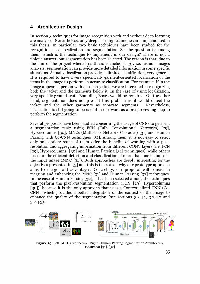
35

4 Architecture Design

In section 3 techniques for image recognition with and without deep learning are analysed. Nevertheless, only deep learning techniques are implemented in this thesis. In particular, two basic techniques have been studied for the recognition task: localization and segmentation. So, the question is: among them, which is the technique to implement in our design? There is not a unique answer, but segmentation has been selected. The reason is that, due to the aim of the project where this thesis is included [3], i.e. fashion images analysis, segmentation can provide more detailed information in some specific situations. Actually, localization provides a limited classification, very general. It is required to have a very specifically garment-oriented localization of the items in the image to perform an accurate classification. For example, if in the image appears a person with an open jacket, we are interested in recognizing both the jacket and the garments below it. In the case of using localization, very specific ground truth Bounding-Boxes would be required. On the other hand, segmentation does not present this problem as it would detect the jacket and the other garments as separate segments. Nevertheless, localization is still going to be useful in our work as a pre-processing step to perform the segmentation.

Several proposals have been studied concerning the usage of CNNs to perform a segmentation task: using FCN (Fully Convolutional Networks) [29], Hypercolumns [30], MNCs (Multi-task Network Cascades) [31] and Human Parsing with Co-CNN techniques [32]. Among them, it is not easy to select only one option: some of them offer the benefits of working with a pixel resolution and aggregating information from different CONV layers (i.e. FCN [29], Hypercolumns [30] and Human Parsing [32] techniques), while others focus on the efficient detection and classification of more than one instance in the input image (MNC [31]). Both approaches are deeply interesting for the objectives presented in [3] and this is the reason why our prototype approach aims to merge said advantages. Concretely, our proposal will consist in merging and enhancing the MNC [31] and Human Parsing [32] techniques. In the case of Human Parsing [32], it has been selected among the techniques that perform the pixel-resolution segmentation (FCN [29], Hypercolumns [30]), because it is the only approach that uses a Contextualized CNN (Co-CNN), which provides a better integration of the context of the image to enhance the quality of the segmentation (see sections 3.2.4.1, 3.2.4.2 and 3.2.4.3).

Figure 19: Left: MNC architecture. Right: Human Parsing Segmentation Architecture.

Sources: [31], [32]

36

4.1 Image Recognition Network

As previously stated, the approach followed in this work is based on merging the concepts of MNC [31] and Human Parsing [32] in a unique architecture. In particular, MNC [31] has been the inspiration for the internal structure of the architecture, creating a network of networks connected cascade-wise. Thus, the design performs multiple tasks (localization and masking) used as learnable pre-processing steps for the final objective: deep pixel-wise segmentation in a Human Parsing [32] fashion, i.e. with a Co-CNN. Depending on the purpose of each of the stages of the network, they could be separated into two generic tasks: preparation for the segmentation (pre-processing module) and the segmentation itself (segmentation module). Please, note that said modules are not physically separated in the network, the separation is only done in terms of the objective of the tasks performed in them.

To sum up, with this architecture the goal is obtaining a multi-task network, based on MNC [31], which performs a pixel-wise classification following the methodology of the Co-CNN presented in Human Parsing [32]. However, rather than simply merging both architectures, the objective is doing it in a more optimal way: reducing the total number of required operations. To fulfil this objective, several changes have been introduced to both architectures; not only to make them compatible, but also to adapt the model to the actual needs of the studied task and enhance its performance. Figure 20 shows a schematic of the proposed network. Its modules and the changes introduced from MNC [31] and Human Parsing [32] are going to be analysed in the following sections.

Figure 20: The proposed network consists of two main modules that perform the different tasks of the network following the multi-task network style presented in [31]. These modules are the Pre-processing and segmentation modules. In the figure, the Pre-processing module appears inside a grey rectangle, where the process of mask generation is performed. The segmentation module appears at the right, with an upsampling and pixel-wise prediction process. This module modifies the particularities from the Co-CNN presented in Human Parsing [32]: Cross-Layer Context (represented with blue arrows) and Global Image-Level Context (represented with green arrows). Both modules are feed with a Shared Convolutional Module: the well-known VGG-16 architecture [34]. For simplicity, the content of the VGG-16 module [34] and some convolutional layers present in the segmentation module are omitted. To analyse in detail the layers inside each module see Section 5. Finally, to facilitate the analysis of the figure, a larger version of the presented image is included in Appendix A.

37

4.1.1 Pre-processing module

As in MNC [31], the proposed architecture is a multi-task network that consists of three different stages: localization, masking and segmentation. Among them, the first two stages are the ones that are part of the pre-processing module. In these stages, despite performing the same tasks than in MNC [31] , only the first module, i.e. RPN, is maintained. In fact, in MNC [31] the localization task is nothing but the RPN, which is clearly improvable. In our approach, it is enhanced in the second stage as it is an active part of the mask creation, which is completely reformulated in this work.

4.1.1.1 Mask creation: Faster R-CNN masking (RoI masking)

In this module, the main objective is the creation of a mask to separate the interesting regions of the images (RoI) from the useless ones (background). This is, in fact, also the purpose of the second stage (see section 3.2.3.2) of MNC [31]; however, the process of creation of the masks is one of the main differences that have been introduced in this work. As explained in section 3, in MNC [31] the masks are represented as an 𝑚2 vector that is regressed to be adjusted to the ground truth mask. However, the problem arises in the fact that the quality of the segmentation in MNC [31] directly depends on the quality of the mask. In fact, note that masking is a binary segmentation (with regions that belong to foreground or background). In the case of MNC [31], the masks aim to do a detailed segmentation of the shapes of the foreground elements (see section 3.2.3.2), which is not an easy task: if it fails, the segmentation is going to be incorrect as the third stage simply labels the foreground masks. The reason why the quality of these masks is in doubt is because they are generated simulating a pixel-wise task but without performing it, as they are computed by the regression of m2 learnable parameters [31]. The problem is that these masks aim to adapt to the shape of the foreground elements, which requires great precision. Nevertheless, without an actual pixel-wise methodology, said accuracy is difficult to be obtained; getting instead only an approximation, which would lead to a deterioration of the quality of the segmentation. Moreover, its application in code is difficult, large and computationally consuming, which also justifies the decision of not using it. Its possible implementation is going to be discussed in future improvements (section 7), as it is beyond the aim of this master thesis.

The solution that has been applied for the masking task has been the usage of an architecture already explained: Faster R-CNN [27]. The original MNC [31], takes advantage of an RPN (Stage 1) for localization purposes. This type of networks is introduced in the Faster R-CNN paper [27] as a pre-processing step from which the actual localization is performed; however, it is not enhanced with the classification/regression architecture that completes a Faster R-CNN [27], i.e. the Fast R-CNN [23] structure; instead, it directly computes the masks from it (Stage 2). In our approach, the Faster R-CNN [27] is completely implemented. This way, in an MNC fashion [31], the first stage

38

continues to be an RPN but the second stage (Stage 2) is replaced by the second module of Faster R-CNN [27]. Then, from the Bounding-Box regression results a mask is generated by setting the pass-band inside the resulting boxes. In this manner, the elements outside the predicted RoIs are going to be filtered (background), focusing the analysis only for the detected meaningful regions (foreground elements, i.e. objects). Figure 21 shows a closer version of Figure 20, focusing on the Pre-processing module explained in this paragraph:

Figure 21: Schematic of the pre-processing module with its integration with the rest of the architecture. Note how the process of masking includes the inclusion of the Faster R-CNN [27] module to compute the Bounding-Boxes results (object detection), from which the masks are generated. In the case of the image, the mask is the black and white rectangle inside the module: the meaningful region (that includes the woman) is the white rectangle (in filters the passband is represented with 1’s, which in grayscale is the colour white) while the background is represented in black (0 in grayscale value). Then the masks are fed into the segmentation module to finish the network. A larger version of the figure can be found in Appendix B.

From the analysis of Figure 21 it could be appreciated how, effectively, the mask is generated from the Bounding-Box output of Faster R-CNN [27], reason why it is referred as RoI mask. Nevertheless, not only the Bounding-Box output is used in the final architecture but also the classification one. In this case, the classification scores are going to be used in the reinterpretation of Image-Level Label Prediction (see section 3.2.4.2). In the figure above it is represented by the green arrow that goes from the classification scores to the Pixel-wise segmentation module, which is represented as a black box as it is going to be presented in the following section.

4.1.2 Pixel-wise Segmentation

The third and final stage of this multi-task network is the segmentation module (see section 3.2.3.3). As previously stated, it is going to be performed following the technique applied in Human Parsing [32], based in a pixel-by-pixel classification with a Co-CNN. This approach replaces the one used in the third stage (Stage 3) of MNC [31], which performs the segmentation as single categorization of the instances given by its second stage (see section 3.2.3.2). To sum up, the segmentation concept is changed from a mask classification

39

into a pixel classification. In the context where the network is integrated [3], the usage of a pixel classification is convenient as it provides a more accurate way of analysing the image: in the fashion world analysis and concretely in fashion recommenders, it is necessary to track the details of the garments, as it may make the difference between different clothes. Working in pixel-resolution allow the segmentation to be as fine-grained as possible, making it a suitable technique for this work. The Human Parsing paper [32] does not implement any kind of methods for determining where is it useful to perform the segmentation task: it is done directly, by a process of classification of the entire number of pixels of the input image. Therefore, a reasonable question could appear: why is it necessary to use a multi-task network if by using single-task network the same results could be obtained? The answer is very clear: efficiency. With the proposed network, once the RoIs are available, the segmentation algorithm is applied only for these regions, which implies that the number of operations to be performed is considerably reduced: from performing a pixel classification of the entire image to applying it only for the meaningful regions. Moreover, the results from the Pre-processing module are useful in the integration with [3], see section 4.2. Figure 22 shows a closer version of the segmentation architecture in Figure 20. The characteristics of this module are presented in the following sub-sections:

Figure 22: Schematic of the Pixel-wise Segmentation module with its integration with the rest of the architecture. In this module, the feature map is upsampled to a pixel-wise resolution from which the segmentation is performed. In the upsampling process, a Co-CNN is applied so as to take into account both the local and global context of the image. In Cross-Layer Context (represented in blue arrows in the image), the equivalent resolution maps obtained in the Shared Convolutional Module (early layers) and in the upsampling process (intermediate layers) are summed, ensuring the presence of both semantic (from the intermediate layers) and local information (from the early layers). In Global RoI-Level Context (green arrow), the scores obtained in Faster R-CNN masking module are converted into a confidence map (green maps in the figure) in the CMap Generator and then are concatenated to the actual maps in order to provide global context to them. Finally, these confidence maps are applied as a correction factor of the final predictions (green sum symbol). A larger version of the figure can be found in Appendix B.

40

4.1.2.1 Cross-Layer Context

Applying Human Parsing with Co-CNN for Segmentation [32] to the MNC [31] strategy implies working in a pixel resolution; otherwise, it is impossible to perform a pixelwise classification. Nevertheless, in a CNN-based architecture, the spatial resolution of the feature maps is reduced as the architecture is deepen. This is the reason why an upsampling is needed: to go back to the original image resolution. However, this cannot be done directly. If so, the obtained feature values would have a lot of semantic information but a lack of spatial/local information, which is essential to perform a pixel resolution task as segmentation is. All these problems are addressed using the Cross-Layer Context from the Co-CNN presented in [32]. In our work, the application of said method remains conceptually the same as in the paper, although some implementation changes are required (see section 5.2.2). In Figure 22, Cross-Layer Context is represented with the blue arrows going from the Shared Convolutional Module to the upsampling process.

4.1.2.2 From Global Image-Level Context to Global RoI-Level Context

Together with Cross-Layer Context, Global Image-Level Context is the main structure present in the Co-CNN introduced in Human Parsing paper [32]. As explained in section 3.2.4, its main purpose is ensuring the coherence between the pixel predictions, i.e. pixel segmentation, and the global image. This increases the quality of the segmentation as the introduction of a global context diminishes the effect of possible outliers. In fact, the presence of outliers is quite common in a pixel-wise classification, as the locations are analysed individually, forgetting their context. For example, the case where the analysed image contains a skirt. When performing a pixel classification, the feature values from a skirt and a dress may be quite similar; therefore, it is likely to obtain the category “dress” as the dominant score in some positions. The introduction of the global context information, i.e. the global label “skirt”, would act as a correction factor, preventing the system from performing an incorrect classification in the analysed position. This task is performed in an inner module represented as the green structure in Figure 22. An important difference with respect to Human Parsing [32] is that, in this work, the internal auxiliary network in charge of the Global Image-Level Context (in green in Figure 18) is no longer used. On the contrary, said task is performed using the predictions already computed by the classification module of the Faster R-CNN [27] architecture, which conforms the pre-processing module of our network, i.e. first and second stages of our multi-task network (see sections 3.2.3.2 and 3.2.3.3). This way, it is possible to take advantage from the classification results of Faster R-CNN [27], that would be otherwise wasted, while supressing the Global Image-Level Context prediction architecture created by [32]. The utilization of the classification results for this task can be appreciated in Figure 21, where it is represented as the green arrow that goes from the classification scores to the pixel-wise segmentation

41

module. In the end, this new architecture implies a reduction of the operations done for this task, increasing the efficiency, which was the objective. In addition, not only the number of layers and operations are reduced but also the network will be now compatible with images from different sizes, as the entire network is performed with Convolutional layers, obtaining a fully convolutional network. This is not the case in [32], where the introduction of FC layers in the network used for Global Image-Level Context requires a unified size for the inputs. Switching from Global Image-Level Context is not only positive in terms of efficiency but also in performance. In fact, the original Global Image-Level Context network computes a general score for the global image. Nevertheless, if more than one instance appears in the input image this approach is not optimal. For example, if in a fashion analysis the input image contains two different models wearing different clothes, the global scores would not be accurate neither for one model nor the other, as the scores for the garments that a model is wearing would be faded with the scores of the garments of the other model. This is the reason why Global RoI-Level Context is introduced. This technique consists in applying individualized confidence values for each of the instances that appear in the image. This is possible to be done due to the usage of the scores obtained from Faster R-CNN [27] instead of Human Parsing’s [32] proposal: while Human Parsing [32] performs the global predictions, our approach computes the confidence values for each of the detected RoIs.

4.1.2.3 Suppression of the Local Super-Pixel Context

The previous sections present the adaptation to the needs of our work of the main tasks performed by the Co-CNN in [32]. Nevertheless, there is a last contextual task that is not going to be applied: Local Super-Pixel Context (represented by the red layers in Figure 18). In it, a set of algorithms are applied to finetune the segmentation results obtained by the rest of the architecture. The main reason why it has not been implemented in this work is because this part of the network requires an external module, which does not fulfill our requirements as it does not apply neural networks. Actually, one of the objectives is having a unique architecture, without external modules. Moreover, the introduction of these module would prevent the architecture from being trainable end-to-end, i.e. Deep Learning, as the results given by these external modules are not learnable. Finally, while it is true that the introduction of the Local Super-Pixel Context enhances the performance of the segmentation task by taking advantage from detailed local information, the characteristics of our architecture compensate its effect. Concretely, with the usage of RoI masks and Global RoI-Level Context, the local analysis is already performed and without the necessity of using non-end-to-end external modules.

42

4.1.3 Shared Convolutional Module

In this work, the final modules of MNC [31] and Human Parsing [32] have been an inspiration for the creation of the pre-processing and segmentation modules. Nevertheless, in both cases, before the application of this final modules, there is a set of Convolutional Layers with the responsibility of dealing with the input data and generating the feature maps from which the described tasks are performed. There are several famous CNN architectures that could be interesting options for the implementation of this Convolutional module: VGG Net [34], Google LeNet [35], Resnet [36], etc. In this work, the Convolutional Layers of VGG16 have been implemented (represented as the cube present in Figure 20, Figure 21 and Figure 22). The reason is that this is the network typically used for MNCs and, moreover, it has available a pre-trained model, which can be useful for the application of a transfer learning technique [56]. Finally, in our approach, due to the implementation of a multi-task network cascade, the feature maps obtained from this convolutional module are going to be used for the different stages of the network, providing shared computation to increase the efficiency of the network. It can be visualized in Figure 20, where there are arrows going from VGG-16 [34] (cube) t0 both pre-processing and segmentation modules. Hence, this is going to be a shared convolutional module.

4.1.4 Integration between modules

Despite the multiple modifications that have been introduced, the integration of the different modules presented in this section does not present relevant differences from the way it is performed in MNC [31]. However, there is a relevant conceptual change that has to be introduced: the suppression of the RoI Pooling Layer in the beginning of the segmentation of MNC [31]. As stated, the MNC’s concept of segmentation [31] differs a lot from ours. In this work, a process of upsampling is needed to return to the original dimensions of the images because otherwise a pixel-segmentation would be impossible. Introducing a RoI Pooling Layer in this context is useless; to begin with, because it would be a pooling that would be created specifically to be destroyed in the following layer via upsampling and finally because it processes the different RoIs separately, losing the compactness provided by the mask. For more details of how the network is finally connected and implemented see section 5.

4.2 Integration with the rest of the architecture

The presented architecture has been designed considering that it is going to be part of the bigger project presented in [3]. In it, the network is set in a recommendation environment: from a real-world image posted in a social network, e.g. Instagram [57], the clothes that appear in it are recognised and matched with similar garments from different online shops, e.g. Zalando [58].

43

However, in an Instagram [57] post the information not only appears in the image but also in the text, reason why it is also a goal of [3] to analyse the information in it. Moreover, the results obtained from these tasks are also used to enhance the image recognition performance, i.e. segmentation. Despite the goals presented in [3] are beyond the scope of this thesis, the current network is going to perform its recognition task. Consequently, our design has to be prepared to support its extension of functionalities. In the following sections, some considerations for the integration of the current design with the tasks performed in [3] are explained.

4.2.1 Integration with image retrieval

For the integration with image retrieval, a set of previous requirements have to be bore in mind: to begin with, the image retrieval between Zalando’s [58] and Instagram’s [57] datasets has to help us in the segmentation task; therefore, where to apply its contribution in the current networks has to be studied. Moreover, an Instagram [57] image could contain instances of garments from different images from Zalando [58]; thus, the system should be prepared to perform a one-to-many process.

4.2.1.1 Image retrieval: a one-to-many process

The main difference between an Instagram [57] image and a Zalando [58] image is that they belong to the real-world domain and the online-shopping domain respectively. In a real-world image, the image will contain, usually, a human wearing its upper and lower clothing. Nevertheless, in an online-shopping dataset, a lot of images do only contain a unique clothing item. The consequence is that performing a matching by comparing the default images from both domains would be inaccurate: the real-world ones, with its several items, would be related to only one instance from the online-shopping domain. Therefore; either the upper clothes, the lower or both of them are going to be incorrectly matched: e.g. an image of a man wearing a jersey and jeans could be matched only with one jeans, making the retrieval partially incorrect. So as to avoid such an issue, the process of matching should be performed not into the entire image but only into clothing instances. Is in this point where the inclusion in the design of a MNC-based architecture [31] results particularly useful. In effect, the first stage of said architecture is an RPN, which proposes Region Proposals where later the rest of the tasks are performed (see section 3.2.3.1). The strategy will consist in training this RPN in order that the obtained Region Proposals correspond to the upper and lower clothing parts of a person. This way, the one-to-many issue is solved and the retrieval design is fitted in the segmentation architecture, sharing all the process until the RPN and getting its own layers for the matching task (e.g. similarity function).

44

4.2.1.2 Integration with the Segmentation task

The idea of image retrieval in this context will provide different useful results. On the one hand, the image retrieval task itself is very interesting as it is always interesting to find the equivalent shopping model of a garment present in the real-world. On the other hand, the information obtained after the retrieval, i.e. the labels from the ideal domain match, are going to be used as a correction factor for the pixel-wise classifiers. The idea is that the information obtained after the matching could give a general context to the pixel decision. This is useful because sometimes when working in a pixel resolution the results obtained could be outliers with no relation with its neighbourhood labels. The presence of this factor of correction is applied by summing said factor in each pixel prediction, preventing this way the proliferation of incorrect spurious results. This process is performed in a similar fashion than the Global Image-Level Context from [32]. Finally, with this contribution to the segmentation task, the image retrieval task not only takes advantage from the segmentation architecture but also contributes to the segmentation task itself. To sum up, the presence of RPN for both tasks and the influence of image retrieval in segmentation makes the process more efficient and physically integrates both tasks in a unique architecture.

4.2.2 Integration with Text Processing

Usually an Instagram [57] image is posted with a description and a set of hashtags that can be useful for the identification of the elements that appear in the image. Taking advantage from said elements could be also very interesting. As in the case of the information obtained after the image-retrieval, the information provided is global context information. Therefore, the proposal is to apply it again as a corrector factor to the pixel-wise predictions for each position.

4.3 RoI pixel segmentation vs. existing architectures

Once the architecture of this work has been presented, it is time to compare it with the architectures studied in the state of the art in order to evaluate its actual worthiness. Concretely, the objective of this section is not performing a technical comparison with the architectures that have been used as an inspiration, which has been already done in the previous sections, but doing it in terms of application: why is it necessary to create a new architecture when there are existing architectures to perform it? The analysis is going to focus in the architectures that have inspired this work: MNC [31] and Human Parsing [32].

45

4.3.1 Comparison with MNC

In the case of MNC [31], the proposed architecture clearly extends its functionalities. Basically, in MNC [31] a detailed garment segmentation as the one presented in [3] would be impossible to achieve. The reason is that the segmentation is performed as a mask classification, i.e. assigning a label to the foreground elements obtained after the masking process. Consequently, it can only segment the foreground elements given by the mask. For example, if an image of a model is introduced to the system, the segmentation with MNC [31] would segment the whole person but not the garments that is wearing, as expected in [3]. On the contrary, our design performs a pixel-wise segmentation, allowing to detect every detail of the analysed region.

4.3.2 Comparison with Human Parsing

There are multiple reasons that makes the new architecture more suitable for our project than directly applying the Human Parsing [32] approach. It could be summarised in the following terms: integration with the rest of the architecture and computational efficiency. To begin with, when it comes to the integration with the rest of the architecture (see section 4.2), the MNC [31] base provides an inner RPN architecture that is going to be very useful for the image retrieval task (see section 4.2.1.1). Moreover, in terms of computational efficiency is where the real gain is obtained. Firstly, the number of operations that have to be performed for both upsampling and pixel-wise classification are going to be considerably reduced. The reason why this happens is because the Human Parsing [32] approach upsamples and classifies the whole pixels of the image, while our methods only perform said task in the computed RoI masks. Moreover, the training of the segmentation module is supposed to be faster. This happens because the pixels outside the RoI are not backpropagated [14]: they are going to be background for sure, reason why backpropagation does not take place (see section 5.2.2.1). Nevertheless, it could be argued that the extra stages of our architecture with respect to Human Parsing [32], i.e. localization and mask creation, suppose an extra number of operations that compensate the ones which are saved when applying a RoI segmentation instead of the analysis of the whole image. But it is not strictly true: to begin with, the Global Image-Level Context network used in Human Parsing [32] is substituted by the results given by the second stage of our approach (see section 4.1.2.2), which supposes the elimination of some layers. Moreover, the remaining extra stage, i.e. RPN, is essential for the integration with [3]. Consequently, the extra stages introduced in our approach substitute parts of Human Parsing paper [32], extend its functionalities and reduce the number of actual segmentation operations, focusing only in meaningful regions of the image, i.e. RoIs. Moreover, the suppression of the auxiliary network responsible of performing the Global Image-Level Context in the Co-CNN of Human Parsing [32], eliminates the usage of effective FC layers, making the architecture compatible with images of different sizes, which is an attractive functionality. Finally, the decision of

46

getting rid of Local Super-Pixel Context, allows to perform an end-to-end training as opposed to Human Parsing [32].

47

5 Implementation

This section explains how the design presented in section 4 has been implemented in our work. The implementation has been done in the Deep Learning library Caffe [38] in a Python programming environment [39]. This section does not present code itself but explains some considerations that have been applied during the elaboration of the code to be consistent with the proposed design.

5.1 Training Input: PASCAL VOC 2012 Dataset

The original idea was using our own Dataset for the implementation. In fact, it would have been the optimal solution as the required annotations for a full development of our architecture would have been available. Nevertheless, the creation of a Dataset is beyond the aim of this thesis. Therefore, the research for an available Dataset that fulfils our needs has been part of this work. Finally, the selected Dataset has been PASCAL VOC 2012 [40]. It presents Bounding-Box annotations which are useful for the localization and mask creation task presented in this work (section 4.1.1.1). Most importantly, this dataset presents also pixel-wise segmentation ground truths, which is basic to perform the segmentation task. However, it presents a couple of problems in that sense. Firstly, PASCAL VOC 2012 [40] has a total of 17125 images, from which only 2913 (divided in training and validation set) have pixel-wise segmentation ground truth [40]. This may result in a problem, as the images available for training are only 1464 [40], which increases the probability of presenting overfitting [54]. Moreover, the aim of this project is doing a pixel-resolution segmentation to detect fine-grained details of the image. Nevertheless, it is not going to effectively happen because, despite presenting a pixel-wise ground truth, the segmentations are presented instance by instance. This is a problem if the objective is performing a detailed fashion analysis like in this project [3]. In fact, with this dataset would be impossible to achieve it, as it does not present enough categories for fashion detection. For example, in the case where the analysed instance is a person, the ground truth label for all its pixels is going to be assigned to the label “person” in PASCAL VOC 2012 [40] (see the figure above), disabling the possibility of capturing details related with the garments.

Figure 23: Example of a ground truth label in PASCAL VOC 2012. Each colour is a different class label. Source: [40]

48

5.1.1 Ground Truth Mapping

In Figure 24 the ground truth label for a PASCAL VOC 2012 [40] image is presented. In it, the different classes are represented with different colours. Nevertheless, an RGB colour is a 3D vector and therefore a 3D label. This kind of labels are not the ones expected by a softmax classifier [20], which usually uses a single index that identifies the category. Therefore, there is the need of performing a mapping from the RGB ground truth to a 1D ground truth of greyscale values. For example, the labels of a person (in pink in Figure 23) are mapped to a greyscale value. The gain is that from a colour represented with 3 values (R, G and B components) we have mapped it into a single value suitable with Softmax. Figure 24 shows the resulting mapping. Note that the new category colours look quite similar. This happens because the greyscale values are selected with consecutive values. Thus, the indexing is easier and better for the system but it is more difficult to perceive the differences for the human eye. As a convention, the black label (greyscale value equal to 0) is reserved for the background category.

Figure 24: Result of a ground truth label after performing the greyscale mapping.

There are existing algorithms that already perform this task; among them, we have used the one presented in [59]. The only major change to introduce is selecting our own data instead of the one used by default.

5.1.2 Problems with the dataset: lack of some box annotations

PASCAL VOC 2012 [40] provides Bounding-Box annotations of their images. This information is essential to perform the localization task present in the architecture presented in this work (section 4.1.1). Nonetheless, some images either don’t present this information or have it damaged. Consequently, when executing a corrupted image in training phase, an error occurs. Unfortunately, it has been impossible to detect the conflictive images rather than during execution. The consequence is that, despite having found out a way to solve this problem, it takes a lot of time to detect and correct the presence of these problematic images. For example, the program can be successfully training for 5 hours until an error occurs due to the lack of box information in the current image. Then, the conflictive image can be erased from the ones used in training and the process can be started again. However, after this time, there

49

can be another conflictive image that stops the process again. Therefore, it could take hundreds of hours to train on the entire dataset. In the work done for this thesis 4 corrupted images have been detected and erased from the trainset. Nevertheless, there are still more conflictive images to be replaced, process which requires more time than the available for the realization of this work. The final consequence of this problem is that the dataset available to perform the Pixel-wise Segmentation, which was already very limited (i.e. 1464 images [40]), has been finally reduced to 225, which obviously implies an important decrease of the potential performance of the network, as shown in section 6.

5.2 Architecture Implementation

After carefully describing the architecture design in section 4, the most relevant details of its implementation are explained in this section. Table 1 briefly reminds the network configuration presented in Figure 20:

Table 1: Architecture Overview

In this thesis, the implementation work has been focused mainly in the Pixel-wise Segmentation. Nonetheless, some changes have been also introduced in the Shared Convolutional Module. Finally, when it comes to the Faster R-CNN Module [27], its code has been directly implemented from [41]. In the following subsections details from the implemented modules are presented.

5.2.1 Shared Convolutional Layers

As stated in section 4.1.3, VGG-16 [34] is selected as the Shared Convolutional Layer module. In column D of Table 2 the VGG structure that has been implemented is shown. Nevertheless, due to that we only use VGG-16 [34] as our Shared Convolutional Layer module, only the first thirteen layers, i.e. the convolutional layers, are implemented.

Architecture Overview

Input: RGB image

Shared Convolutional Layers

Faster R-CNN

Pixel-wise Segmentation Module

50

Table 2: Architecture of each of the VGG architectures. The selected in this work, VGG-16,

appear in column D. Source: [34]

VGG-16 [34] is a well-known CNN architecture that has been widely used in works like MNC [31] or Human Parsing [32]. Its main drawback is that it is a huge network, with a lot of layers. For instance, VGG-16 presents 138 million of parameters [34]. Nevertheless, the weights trained using ImageNet [42] are available on-line. This is very useful for applying a Transfer Learning technique [56], which consists in applying to a network available weights from a pretrained model, typically trained using ImageNet [42] dataset, and then fine-tune its values to adapt to the desired dataset in each case. The use of Transfer Learning [56] saves a lot of time and reduces the computational costs. Theoretically, it is a technique which is suitable for a work like the one presented in this thesis. However, in practical terms, VGG-16 [34] is a huge CNN architecture which, despite applying Transfer Learning [56], gives trouble in terms of memory when running the execution in the server. Concretely, the problems arise when working with the larger layers from VGG-16 [34], where 512 different filters are applied [34]. The implemented solution has consisted in applying a simpler and smaller architecture: AlexNet [37], presented in Table 3:

component type kernel

size/stride output

channels

Shared Convolutional

Module

Convolution 5 x 5 / 1 96

Max Pooling 2 x 2 / 2 96

LRN normalization

- 96

Convolution 5 x 5 / 1 256

51

Max Pooling 2 x 2 / 2 256

LRN normalization

- 256

Convolution 3 x 3 / 1 384

Convolution 3 x 3 / 1 384

Convolution 3 x 3 / 1 256

Max Pooling 2 x 2 / 2 256

Table 3: AlexNet Configuration. Source: [37]

The approach in Table 3 presents the classical AlexNet configuration [37]. However, in our approach, the padding parameter (see section 2.1.1.2) has been changed so as to ensure that the sizes of the input images are not changed in the Convolutional Layers but in Max Pooling layers. Concretely, in this case, padding is set to 1 and 2 when the receptive field is 3 and 5, respectively [8]. In addition, it must be noted that the output channels column refers to the depth dimension of the resulting feature maps in each layer, i.e. the number of filters applied in the Convolutional layers. In fact, this was the conflictive parameter when using the VGG-16 configuration [34]. However, switching to an AlexNet-based configuration [37] reduces the maximum value for this parameter from 512 to 384, which can be handled with the server used in this thesis [37]. On the other hand, the reason why in Table 3 the height and width are not specified is because it depends on the dimensions of the input image, which is variable in our design: due to the usage only of Convolutional Layers in the design (fully convolutional network), images from different sizes can be handled by this network. Moreover, as opposed to VGG-16 [34], AlexNet [37] includes batch normalization layers [43]. The use of this type of layers compensates an incorrect weight initialization, which is one of the main difficulties that could appear when training a neural network. In that sense, it is important to note that the Convolutional Layers have their weights initialized following a gaussian distribution [44] of mean 0 and a standard deviation of 0,01; which, in principle, is a good way to initialize the weights of the network [46]. Finally, note that for simplicity the ReLU activation functions [18] after each Convolutional layer have not been included in the Table. The results presented in this thesis (section 6) are obtained with our modified version of AlexNet [37], which has an important consequence: Transfer Learning [56] is no longer a feasible option. The reason why this happens is because, after modifying the network, our required number of parameters differ from the weights from pre-trained AlexNet-based models [37] available on-line. Thus, the network has been trained from scratch, which increases the training time. Despite this problem, the impossibility of using the pretrained VGG-16 [34] due to server limitations has forced the implementation of this suboptimal solution.

52

5.2.2 Pixel-wise Segmentation Module

This section introduces the implementation details related to the Pixel-wise Segmentation module described in section 4.1.2. Despite this module is based in the architecture described in [32], their implementation is not available neither on-line nor contacting with the authors. Consequently, it has been implemented from scratch in this thesis, including the creation of new layers and the selection of the required parameters in order to fulfill the changes introduced in our design with respect to the state of the art, i.e. Faster R-CNN or RoI masking, dimension changes in Cross-Layer Context and Global RoI-Level Context. A summary of the layers used for each task and its more relevant parameters are presented in Table 4:

component Type kernel

size/stride output

channels

RoI masking

Python: RoI mask data

- 256

Python: RoI masking

- 256

Global RoI-Level Context

Python: RoI CMap Generator

- 21

Cross-Layer Context

Deconvolution 4 x 4 / 2 256

Convolution 5 x 5 / 1 256

Crop - 256

Element sum - 256

Concatenation 277

Convolution 5 x 5 / 1 256

Deconvolution 4 x 4 / 2 256

Convolution 3 x 3 / 1 256

Crop - 256

Element sum - 256

Concatenation - 277

Convolution 5 x 5 / 1 256

Deconvolution 4 x 4 / 2 256

Convolution 5 x 5 / 1 96

Crop - 96

Element sum - 96

Concatenation - 117

Convolution 5 x 5 / 1 96

53

Convolution (image)

5 x 5 / 1 96

Crop - 96

Element sum - 96

Convolution 3 x 3 / 1 256

Prediction

Python: RoI masking

- 256

Convolution 1 x 1 / 1 21

Crop - 21

Element sum - 21

Convolution 1 x 1 / 1 21

Python: RoI masking

- 21

Python: CMap Element sum

- 21

Ground Truth Masking

Python: RoI masking

- 1

Table 4: Pixel-wise Segmentation Module Configuration. This table presents in detail the

components presented in Figure 22

In Table 4, there are 4 columns that describe the module configuration. To begin with, “component” specifies the global task performed by the stack of layers included in each of the blocks in the Table. Then, “type” specifies the type of Caffe layer which is used in each case. In the cases where the layer has been created specifically for the realization of our architecture, the type which appear in the Table is “Python”. Finally, “kernel size/stride” and “output channels” refer to typical parameters to be introduced in Convolutional layers. Like in Table 3, “output channels” refers to the depth dimension of the obtained feature maps in each of the layers. Again, the output width and height are not specified as they vary depending on the input image. This happens because the limitation in a CNN in terms of size is given by FC layers: while Convolutional Layers operate exactly in the same way with different input sizes, FC layers need always inputs of the same size. The suppression of FC layers in the design allow the network to be compatible with any input size, reason why width and height are not specified in the table. Finally, note that for simplicity the ReLU activation functions [18] after each Convolutional Layer have not been included in the Table. The architecture presented in Table 4 corresponds to the training configuration. Concretely, the only thing that must be changed for the test is erasing the last component, i.e. Ground Truth Masking, as this is a layer that contains ground truth information (not possible in test environment). The type of layers used in each task is consistent with the elements described in sections 4.1 and 3.2.4. Note that, despite its name is not very clear, Caffe

54

Deconvolutional layers [45] are in charge of performing the upsampling task necessary to perform a Pixel-wise Segmentation. In that sense, it is important to ensure that the dimensional changes only take place in the upsampling layers. Hence, Convolutional layers are set to not modify the size of the input feature map, selecting the padding to maintain the dimensions, i.e. 1 and 2 when the receptive field is 3 and 5 respectively [8]. On the other hand, its weights are filled following a gaussian distribution [44] with 0 mean and a standard deviation of 0,01. Thus, the problems related with initializing with zeros the weights are avoided [46]. In Global RoI-Level Context component, the created layer RoI CMap Generator implements the functions described in section 4.1.2.2: from the scores generated in the Faster R-CNN [27] module a confidence map is created per each RoI (represented as the green maps in Figure 20 and Figure 22). Furthermore, note how in the beginning of the prediction component, a RoI masking is performed again. This is done to ensure that during the process of upsampling, due to the convolutional layers (which depending on the parameters change the dimensions of the input, see section 2.1.1.2), the predictions are not also performed outside the region to be analysed, i.e. RoI. Finally, layers for performing Ground Truth Masking (see section 5.4.1.1), CMap Elementwise Sum (see section 5.2.2.1) and Crop (see section 5.3) are introduced to solve implementation issues which are going to be described in detail in the following sections.

5.2.2.1 Prediction processing

One of the advantages of our approach is that it only performs the prediction for the meaningful regions of the image, i.e. the previously detected RoI (see section 4.1.1.1). Precisely due to RoI masking, the background elements are not processed and are assumed to be directly background. Nevertheless, as it is shown in Table 4, in the final layer are obtained as many predictions maps as analysed categories (21, as it is the number of categories in PASCAL VOC 2012 [40]). The process is easy to understand, as explained in section 2.1.1.2, the output of a CNN has as many channels as applied filters. In the final layer, the number of filters applied are just as much as the number of categories to analyse. Therefore, the obtained prediction maps have the width and height size of the image (remember that we aim to do a pixel-resolution classification) and as many channels as categories. This means that one of these category maps is the one related to background. The problem with background is that its regions are not analysed due to the RoI masking. However, the ground truth label does have background annotations, therefore it expects that in the positions where there is background its category map presents a score different from zero, which is not the case due to RoI masking. To solve this, in the background regions of the background category map a fixed confidence value is set. This value has been selected to be 20 as it is large enough to avoid the backpropagation (i.e. learning process) for these positions (where we have nothing to learn as we already know that they belong to the background). Sections 5.5 and 5.5.1 present this process using figures.

55

5.3 Size incompatibility during Upsampling

During the Shared Convolutional Module, 3 Max-Pooling layers are introduced (see Table 3). These layers are responsible of downsampling the dimensions of the inputs of a CNN. The reduction of dimensionality allows to easily handle the initially huge dimension of input images and, moreover, provide the generalization required to perform a classification analysis. Nevertheless, as explained in sections 3.2.4.1 and 4.1.2.1, to perform a Pixel-wise segmentation it is necessary to work with the original resolution of the image, which implies the necessity of upsampling the feature maps to the original image dimensions, and taking into account the context of the intermediate layers to enrich the feature maps with spatial/local information. This is performed by doing elementwise summation (see Table 4) between the upsampled feature map and the resolution equivalent intermediate layer feature map. Here is where the problem arises: if the two different feature maps do not present the same dimensions, the elementwise summation is not possible. Unfortunately, the presence of odd values for width and height provokes this dimension incompatibility. In the following sub-section, an example showing these difficulties is presented.

5.3.1 Upsampling incompatibility example

In this example section, it is going to be supposed that the input dimensions in the network is 331, i.e. an odd number. The downsampling process takes place in the Shared Convolutional Module; therefore, in this example, the Max-Pooling parameters used in Table 3 are going to be applied. To begin with, the formula applied in Max-Pooling has to be reminded:

O = (𝐼 − 𝐹 )

𝑆 + 1

Where I and O refer to the input and output dimension, respectively; F, to the receptive field (kernel size) and S to the stride [8]. In this case, I=331 and, following Table 3, F=S=2. Therefore:

O = (331 − 2 )

2 + 1 = 165.5

Obviously, the dimensions that must be handled in the program have to be integer values. This is the reason why the Pooling built-in Caffe layer [47] applies the following formula:

O = 𝑐𝑒𝑖𝑙 ((𝐼 − 𝐹 )

𝑆+ 1)

56

Where ceil is the built-in Python function that rounds a float value to its immediately higher integer value [48]. Consequently, in the studied example, the output dimension is the following one:

O = 𝑐𝑒𝑖𝑙 ((331 − 2 )

2+ 1) = 166

Following the entire architecture in Table 3 and the formula previously shown the dimension evolution for an input of size 331 would be the following:

331 166 83 42

Then, the Pixel-wise Segmentation Module starts and the dimensions are upsampled by a factor of 2 to go back to the original image resolution:

42 84 168 336

Analysing the previous evolution it is highlighted how the dimension for equivalent resolutions no longer matches. For example, it would be impossible to perform the required elementwise summation between the third resolution elements (i.e. the one obtained after two Max-Pooling layers) as the dimensions are 83 in the downsampling process and 84 after the upsampling one. This difference of size happens due to the rounding factor introduced by the built-in Python function “ceil” in the Pooling built-in Caffe Layer. Concretely, the presence of this rounding factor disables the possibility of going back to those dimensions whose actual value when being halved in the downsampling process is not an integer value. The solution for this problem is presented in the following section.

5.3.2 Solving Upsampling incompatibility: Crop Layer

To solve the problem presented in the previous section, the Crop built-in Caffe Layer [49] has been introduced in the architecture. Note how, in the Cross-Layer Context component in Table 4, between each Deconvolutional and Elementwise summation layer, a Crop Layer has been introduced. This Layer ensures that, when applying Cross-Layer Context, the dimensions of the feature maps used in the Elementwise summation match. Consequently, after introducing the Crop Layers, the aforementioned dimension evolution goes as follows:

331 166 83 42 84 Crop 83 166 332 Crop 331

It can be seen how the application of two Crop Layers correct the incorrect upsampled values. Thus, the required dimensions to allow an elementwise summation to fulfil the Cross-Layer Context applied in the architecture are obtained.

57

5.4 Learning configuration: multi-task single-stage learning

In section 4, where the design of the network is presented, the tasks performed by the network are explained. Concretely, it is explained that, despite being the main purpose of the network the computation of the pixel-wise segmentation of the input image, there are other useful tasks that have to be performed to fulfill the final goal: the computation of RoI, which are later used as masks from which the segmentation takes place. Therefore, as this design performs more than one task, it can be referred as a multi-task network. These networks can be trained (end-to-end) in two different ways: single-stage or multi-stage training. The difference between these training methods is that in multi-stage training each of the tasks have their own loss function, which is optimized separately from the others, i.e. the training is done sequentially: optimizing first one task and then the others. For example, in the presented design, a multi-stage training would imply training first the Faster R-CNN [27] module to generate the RoI masks and, later, taking the trained values for this module performing the Segmentation Module training. On the other hand, in single-stage training, a unique loss function, also known as multi-task loss function, is used. Typically, a multi-task loss function is nothing but the summation of all the individual loss functions. With multi-task loss functions, the training process for all the tasks is performed in parallel, at the same time (joint learning). Thus, in this work, it would not be necessary to train first the Faster R-CNN [27] module and then the Pixel-wise Segmentation module: it is done together in a single-step. This solution is the one selected for this work as it is more elegant, more compact and faster. Figure 25 shows how the single step training behaves:

Figure 25: This figure shows a simplified version of the proposed architecture specifying its loss functions and how backprop goes through the different modules. 𝑳𝒎𝒂𝒔𝒌 refers to the loss function of the Faster R-CNN masking module and 𝑳𝒔𝒆𝒈 to the one of segmentation. Finally,

𝑳𝑻 is the multi-task loss function. The derivative forms of the different losses are referred with

an apostrophe, e.g. 𝑳𝒔𝒆𝒈′ is the gradient of 𝑳𝒔𝒆𝒈 with respect to the weights in the segmentation

module.

58

In this architecture, each module is only responsible of optimizing itself, i.e. the training process of the Segmentation Module does not contribute in the optimization of RoI masks generation in Faster R-CNN [27]. In practical terms, this consists in assuming the RoI masks as fixed inputs of data introduced to the Segmentation Module. The data given to a neural network, the Segmentation module in this case, cannot be changed during the learning process. In mathematical terms, this implies that the loss function of the Segmentation module is independent of the RoI generation, as the generated RoI masks are considered as invariable data. It is shown in Figure 25, where the two different modules backpropagate only the gradients of their individual loss functions. This happens because each module only differentiates with respect to their weights, which apply only in their individual loss function, reason why the other loss term disappears (as it is seen like a constant term with respect to the specific weights of each module). In some cases, like in the loss function of Faster R-CNN [27], there can be found dependent loss functions in multi-task networks, i.e. the loss function depends not only on the weights of their task/module but also on the weights of another tasks/modules. The main reason why it is not applied in this work is because dependent loss functions have to be differentiable with respect to the all the dependent modules, which in Figure 25 would imply that 𝐿𝑠𝑒𝑔

′ was also

backpropagated through the Pre-processing module. Unfortunately, in this work, the dependency between modules is given in RoI Masking (see Figure 25). In it, the masks are generated in a thresholding process, i.e. ones inside the computed RoI and zeros outside, which is a non-continuous function and therefore non-differentiable [50]. Moreover, dependent loss functions are especially useful when the tasks performed in the different modules are related. For example, in the case of Faster R-CNN [27] the dependency is applied between the loss function of RPN and the one from the final Bounding-Box regressor, which precisely refines the values given by the RPN. Therefore, there is a clear connection between the tasks. On the contrary, in the design presented in this work, the tasks performed in Faster R-CNN [27] and in Segmentation module are totally independent: localizing objects and classifying pixels. This means that including the relation of dependency between their loss functions is not essential as it does not help significantly in the optimization of the RoI masks (because in a process of classification the operations to regress a RoI are not performed). In addition, the non-dependency relation between modules should not affect the network in terms of its quality as Faster R-CNN [27] is the most well-known localization algorithm using CNNs, reason why, when correctly trained, provides excellent data that can perfectly be used as a fixed input in the Segmentation module. However, although it is not strictly necessary in this work, the inclusion of a dependent loss function between Segmentation and Faster R-CNN modules could be interesting and might be considered in Future Work as it makes the design more elegant and precise. On the other hand, due to the differentiation rule that establish that the derivative of the summation is the sum of derivatives, the weights that are common for both tasks, i.e. only the ones used in the Shared Convolutional Module, consider the gradients coming from

59

both individual loss functions [50] (see Figure 25). Thus, the training of both tasks is performed in parallel, taking advantage of the shared computation that the Shared Convolutional Module offers and performing a single-step training.

5.4.1.1 Ground Truth Masking

One of the main consequences of fixing the RoI masks as inputs to the Segmentation module is the necessity of ensuring that the loss of this module does not take into account the losses given by an incorrect mask generation: as the masks are considered fixed data the segmentation module cannot improve them. In this section, the solution implemented to solve this issue is presented. As it can be seen in Table 4, just before the start of the prediction step, there is the masking of the Ground Truth image. The mask which is used is exactly the same that has been previously applied to the feature maps. The reason why this is done is to ensure that we are only evaluating the predictions that have been done in the Segmentation module. As stated in section 4.1.2, in this module the operations are only performed in the precomputed RoIs. Therefore, the evaluation is also only performed at these regions. In practical terms, masking the ground truth implies assuming that the RoI masks generated (see section 4.1.1.1) in the architecture give perfect results, i.e. that all the filtered regions are background. In principle, it is not necessary true: if the masks are incorrectly generated it is possible that some foreground elements or parts of them get outside the RoI, which implies that they are going to be incorrectly masked. Nevertheless, it is one of the consequences of fixing the masks: they must be considered as correct data. Therefore, masking the ground truth supposes trusting in the RoI masks (even when they have been incorrectly generated). The consequence is that we would be optimizing the predictions in the analysed regions, even though they have been incorrectly generated. To sum up, the idea behind this is allowing the training only for the predictions that have been really computed in this module, i.e. the segmentation prediction of the elements inside the RoI; without caring, in this stage, about the quality of the generated RoI masks, as its generation is not responsibility of this module but of the Faster R-CNN masker, which is also conveniently trained. Note that Ground Truth Masking is especially useful in the beginning of training, when the masks are not still correctly generated. In that moment, the loss of the segmentation module would be really large independently of the actual operation of this module and making difficult the visualization of the actual problems of the module. On the other hand, when the network is trained, the RoI masks increase its accuracy making irrelevant its presence.

60

A visualization of the process of Ground Truth Masking and its consequences are shown in section 5.5.2.

5.5 Visualization of the prediction process

Let’s imagine the case where after the first RoI masking layer of the prediction component of Table 4, the feature map presents the following dimensions: 2 ×2 ×1 (hypothetical case to make a simple example). At this point, all the process described in 4.1 has been completed, obtaining a pixel-resolution map with values containing both semantic and local information. This feature map is represented in the following figure:

29 0

0 93

Figure 26: Visualization process: feature map

Note that the regions where the value is 0 are those that has been masked in the RoI masking process. In other words, in this concrete example, the RoI would be the pixels in the position (0,0) and (1,1) while the others are considered background and therefore masked (value to 0). All the maps presented in this section are going to present 0 values in the masked position, coherently with the operation of our design, which only works in the meaningful regions (see section 4.1). From this moment, the prediction process starts. In the context of segmentation, the prediction step consists in assigning to each pixel a category. In training step, it is necessary to have a ground truth image that is going to be the reference from which the accuracy of the predictions is evaluated. The following figures represent the original RGB ground truth image with three categories, i.e. C1 (blue), C2 (green) and Background (black), and how we map it into a greyscale representation with the process described in section 5.1.1.

Figure 27: Visualization process: ground truth mapping

C1 BG

BG C2

1 0

0 2

61

Note that from RGB values we have switched to greyscale values, associating the labels to a single index: BG = 0, C1 = 1 and C2 = 2. Once the ground truth is available, the prediction process starts. Following the process explained in section 2.1.1.2; from the input map, as many confidences maps as the number of available categories are going to be predicted (as the number of filters is going to be the same as the number of categories to predict):

Figure 28: Visualization process: prediction maps

Note that, for simplicity and clarity, the prediction maps obtained for each of the categories are represented with the colours that have been used in the ground truth label example, i.e. black for Background, blue for C1 and green for C2. With the predictions scores computed, it is time to apply Softmax classifier with loss [20]. What a Softmax classifier does is simply converting the obtained scores into probabilities following this formula:

𝑝𝑖,𝑗,𝑐 =𝑒𝑠𝑖,𝑗,𝑐

∑ 𝑒𝑠𝑖,𝑗,𝑐′𝑐′∈𝐶

Where 𝑝𝑖,𝑗,𝑐 is the probability of the pixel in the position (i, j) of being

assigned the label of class C and 𝑠𝑖,𝑗,𝑐 is the score obtained in the prediction

maps shown at Figure 28. Then, in training step, these probabilities are used to compute also the loss function. Typically, with Softmax classifier, it is applied a logarithmic loss function:

𝐿𝑖,𝑗 = −𝑙𝑜𝑔 (𝑒

𝑠𝑖,𝑗,𝑐𝑔𝑡

∑ 𝑒𝑠𝑖,𝑗,𝑐′𝑐′∈𝐶

)

This function is applied at each position (i, j). Note that in the numerator it is only used the score for the correct category, i.e. the score obtained in the prediction map of the ground truth category [20]. In the following figure a

4 0

0 10

22 0

0 92

29 0

0 93

76 0

0 12

62

calculation examples for two positions of the previous figures is going to be shown:

Position (0, 0)

Ground Truth: Prediction Maps:

𝐿0,0 = −𝑙𝑜𝑔 (𝑒76

𝑒4 + 𝑒76 + 𝑒22) = 0

Figure 29: Visualization process: position evaluation I

From this example, it can be seen that the prediction in the position (0,0) is very good (the score for the correct category is higher enough than the scores for incorrect categories). Therefore, the loss is inexistent. When this happens, the system cannot learn anything from this position: the learning algorithm of a neural networks starts from the loss function, trying to minimize its values. When the value is 0 there is nothing to learn and the process does not start (it does not backpropagate, the gradient is going to be 0 or almost 0) [13][14].

Position (0, 1)

Ground Truth: Prediction Maps:

𝐿0,1 = −𝑙𝑜𝑔 (𝑒0

𝑒0 + 𝑒0 + 𝑒0) = 1.098

Figure 30: Visualization process: position evaluation II

This is the specific situation described in section 5.2.2.1. As explained, in this design only the meaningful regions are used for the prediction task. These meaningful regions are given by the RoI masks previously applied. In this case, the positions (0,1) and (1,0) are masked, which in practical terms means

C1 BG

BG C2

4 0

0 10

22 0

0 92

76 0

0 12

C1 BG

BG C2

4 0

0 10

22 0

0 92

76 0

0 12

63

that they contain background. As we already know that these positions contain background, they do not take part of the prediction and consequently there are no scores obtained in these positions. However, the loss function is going to be applied and, due to the lack of scores in these positions, the loss is going to be different from 0. Which means that, eventually, a learning process with backpropagation would start from this point. This is something that is not desired in this design, as the classification for these background positions has been already done in the mask generation and it would be a waste of resources to start a process of learning again. The solution to solve this issue is presented in 5.2.2.1 and shown in the following section.

5.5.1 Prediction processing: correcting the Background score

As explained in 5.2.2.1, the proposed solution has consisted in applying a constant value to the masked positions of the Background category map. Thus, the required score for these positions is obtained. Concerning the value to apply, with a sufficiently large number, e.g. 20, is enough, as the rest of scores for the other category maps would remain to 0. It is shown in the following figure:

Ground Truth: Prediction Maps:

𝐿0,1 = −𝑙𝑜𝑔 (𝑒20

𝑒20 + 𝑒0 + 𝑒0) ≈ 0

Figure 31: Visualization process: correcting the background

Correcting the score the loss falls to 0, preventing the learning to start, which gives sense to the RoI prediction, reducing the number of prediction operations.

5.5.2 Ground Truth Masking visualization

In section 5.4.1.1 the process of Ground Truth Masking is shown. For explaining its importance, it is needed to focus on a particular case: when the RoI mask has been incorrectly computed. Typically, this happens in the

C1 BG

BG C2

4 20

20 10

22 0

0 92

76 0

0 12

64

beginning of the process of training, when the obtained results, i.e. masks in this case, are still improvable: Correct Mask: Predicted mask: Ground Truth:

Figure 32: Visualization process: incorrect mask generation

The figure above shows how the predicted mask mismatches the label for the position (1,1,). This position is filtered considering that its label is Background when in reality it is C2. As stated, the process of Pixel-wise Segmentation consists in classifying the pixels inside the generated RoI mask, even if this has been incorrectly computed. On the other hand, the regions masked are directly considered background and do not go through the process of classification. In the ideal case where the RoI mask is correctly computed, this is not an issue but if the mask is incorrectly generated it gives problems. The following figure shows it:

Ground Truth: Prediction Maps:

Figure 33: Visualization process: prediction with incorrect mask and background not

corrected

After correcting the background scores as explained in 5.2.2.1 the obtained prediction maps are the following:

Ground Truth: Prediction Maps:

Figure 34: Visualization process: prediction with incorrect mask with background correction

FG BG

FG BG

FG BG

BG FG

C1 BG

BG C2

C1 BG

BG C2

4 0

27 0

22 0

4 0

76 0

8 0

C1 BG

BG C2

4 20

27 20

22 0

4 0

76 0

8 0

65

Analysing the figures above, it is clear that the problem is given in the position (1,1) where the background presents the maximum score despite the fact that its real label its C2.

Position (1, 1)

Ground Truth: Prediction Maps:

𝐿1,1 = −𝑙𝑜𝑔 (𝑒0

𝑒20 + 𝑒0 + 𝑒0) = 20

Figure 35: Visualization process: evaluation with incorrect mask with background correction

The consequence of the incorrect mask is clear: the loss value is huge. Nevertheless, this cannot be corrected, because we cannot correct a prediction that has not been generated in this stage: even if backpropagation takes place, the only way to solve this problem is by changing the RoI mask, which is not responsibility of this loss function (remember that RoI masks are fixed for the segmentation task. See section 5.4). Here is when the Ground Truth Masking takes place. After masking the ground truth, it looks like this:

C1 BG

BG BG

Figure 36: Visualization process: ground truth masked

Ground Truth: Prediction Maps:

C1 BG

BG C2

4 20

27 20

22 0

4 0

76 0

8 0

C1 BG

BG BG

4 20

27 20

22 0

4 0

76 0

8 0

66

Figure 37: Visualization process: evaluation with ground truth masked

Thus, the problem is partially solved: the loss function of the prediction step is not going to be in charge of a mistake which does not depend of its performance but of the RoI mask generation. However, in reality, the original mistake, i.e. the incorrect mask generation, still is going to take place. Ground Truth Masking simply fools the system to allow, exclusively, the evaluation of how the pixel-wise classification work but not how the RoI has been generated, as this task has its own loss function. This happens because the RoI masks are assumed as fixed in the segmentation process. Summarizing, Ground Truth Masking prevents the architecture from considering the losses given by an incorrect mask generation not only in the loss function of the RoI mask generator but also in the Segmentation module, which is not responsible of these mistakes. As stated, this is particularly important in the beginning of training, when the generated masks are not still very accurate. Once the architecture is globally optimized, the generated RoI masks are better and Ground Truth Masking becomes irrelevant.

5.6 Server selection

The selection and preparation of the server has been a clear limitation factor in this project. To begin with, there were some difficulties in the configuration of the server that affected the time available for the implementation. In the end, an AWS [51] used. Nevertheless, the capacity of the contracted server does not fulfill the requirements of this project. Due to its lack of capacity, it has been necessary to introduce some changes to the original architecture. The most important one is the change from a VGG-16 architecture [34] to AlexNet [37], which clearly reduces the performance of the entire network, as AlexNet [37] is a much more simpler architecture than VGG-16 [34] (see section 5.2.1). Thus, with less layers and operations, the obtained feature maps after the Shared Convolutional Module are not accurate enough, reducing the quality of the generated RoI and, consequently, of the pixel-wise segmentation. In addition, the change to AlexNet [37] and the changes introduced to it (see Section) do not permit to use Transfer Learning [56], which was a convenient option for this project. On the other hand, some additional work has been necessary to be done with the dataset. Concretely, the images have been reshaped as their original dimensions were too big to be handled (out of memory error) by the contracted instance of the server. This, despite looking as a simple issue, has implied an important analysis of how image information is handled in [41] and its modification to adapt it to the server capacity, being necessary the creation of some additional functions during this process. Therefore, to sum up, the initial difficulties to find a server to work with and the limited capability of the selected instance delayed the execution of this project.

67

6 Results

This section aims to present the results obtained for the segmentation task during the testing phase so as to prove that the proposed network has been successfully implemented and that it is ready for working. The reason why it has been decided to focus on the segmentation task despite being the presented network a multi-task architecture is because the rest of the tasks are implemented through a module, Faster R-CNN [27], which has been widely tested in the state-of-the-art, reason why there are no doubts of its correct implementation. Moreover, the evaluation metrics, testing conditions and finally an analysis of the results are also included in the following sections. Note that this section does not aim to evaluate the proposed network with respect to other well-known architectures, as it is beyond the scope of this thesis.

6.1 Evaluation metrics

In the evaluation, three basic metrics are going to be presented: accuracy, precision and recall. When it comes to accuracy, in this case it would be considered as simply the percentage of pixels which are correctly classified by the Pixel-wise Segmentation network. Precision, recall and F-1 score [52] are also going to be computed as they are going to provide a measure of the quality of the obtained results.

6.2 Testing conditions

As explained in section 5.1, the models are trained on PASCAL VOC 2012 [40] training set and evaluated on the evaluation set. Nevertheless, as shown in section 5.1.2, due to problems with the dataset the trainset has been reduced from 1464 to 225 images, which is an important reduction. Moreover, due to the fact that training images are selected randomly during the training, it has been not possible to monitor which images were the 225 which were not giving trouble. This is an important point, because due to this problem the train has been done only for 225 iterations, as it is impossible to complete an epoch in the actual dataset without obtaining errors. In the end, the trained model would be the equivalent of the one obtained after training for a single epoch a dataset with only 225 images. Concerning the testset, due to the limited capacity of the server, the images were too big (giving an out of memory error) and have been reshaped to smaller dimensions. The process of training is performed using an instance of an AWS server: [51] (see section 5.6). Using this server and the available sample of PASCAL VOC 2012 [40] the network has been trained following the learning configuration presented in the following section.

68

6.2.1 Definition of the learning parameters

In Caffe [38], the training parameters are defined in “solver.prototxt”. In this file, parameters related with the learning process are defined. One of the main elements to select is the optimizer. There are several options: SGD, Adagrad, Adam, etc. [15][16] Among them, SGD [13] has been applied. It has been selected as it was the optimizer used in [41]. In this work the base learning rate has been set to 0,001. However, fixing the learning rate is not optimal, as depending on the moment of training the learning rate should present higher or lower values [15][16]. To solve this issue, an exponential weight decay is applied (weight_decay = 0.0005). Thus, the original fixed learning rate is exponentially reduced: this way, in the beginning of the process, when there is still a lot of things to improve, the learning steps can be larger (less precise) and while the architecture gets trained, the steps are progressively reduced to be more accurate. Moreover, a momentum factor of 0,9 is also applied. Remember that this factor is applied to speed up the training algorithm in presence of saddle points, i.e. points where the gradient gets stuck, progressing really slowly. The inclusion of the momentum factor helps going through these points, which enhances the performance of the training [15][16]. Finally, the batch size during training includes only 1 image, performing an on-line training [13].

6.3 Numerical results

Taking into account the conditions presented in section 6.2, the results obtained after testing the trained model are summarized in Table 5:

Avg. Accuracy Avg. Precision Avg. Recall Avg. F-1 score

25.09 47.62 15.09 22.93

Table 5: Results obtained in % after evaluating the network

Due to dataset and server limitations the results were not expected to be good and this is what can be appreciated in Table 5. The accuracy is only of 25% which represents a really low value. The average precision is also considerably improvable. Although its value might look better it must be noted that precision and recall always have to be evaluated together: precision only indicates the percentage of pixels classified with the same category that are correctly classified, while the recall specifies the percentage of actual pixels of a class that are correctly classified. In this case the recall is only of 15%, which reaffirms that the obtained results are far from optimal. In order to analyse both precision and recall together, there are metrics like F-1 score that combine both metrics, presenting again an improvable result of only 22.93%. Finally, it must be noted that an incorrect initialization that negatively impacted to the results has been corrected. In the beginning, the weights were

69

set to 0, which is not an advisable practice as it usually gives bad performance. After detecting said problem, the weights were initialized following a gaussian distribution [44] with 0 mean and a standard deviation of 0.01 (see section 5.2.2) [46]. After these changes, the performance was enhanced. Moreover, the introduction of Ground Truth Masking also improves the performance of the system as it can be visualized in section 5.5.2. An accurate analysis of why the results are so bad is presented in the following section.

6.3.1 Analysis of the results

The low results obtained by the proposed design are responsibility of two main elements: the dataset and the limited capabilities of the selected server. Due to the characteristics of the task performed in this work, i.e. pixel-wise segmentation using Co-CNN, the architecture from the state of the art which is more suitable for a comparison is the one presented in [32]. A theoretical comparison between the networks is presented in section 4.3.2. Unfortunately, when it comes to the performance, it is no possible to do it in fair terms as the implementation of [32] is not available neither on-line nor contacting with the authors. Therefore, it is not possible to test this network with the same conditions used in our network. Anyway, and although it is not the aim of this thesis to compare our network with pre-existing architectures, it is interesting to have a look at their obtained results:

Avg. Accuracy Avg. Precision Avg. Recall Avg. F-1 score

97.06 87.83 81.73 83.78

Table 6: Human Parsing Results. Source: [32]

It is clear that the results presented in Table 6 outperform the ones presented in Table 5. As stated, it would be unfair to compare them because the conditions used in both cases are totally different. Nonetheless, comparing the testing conditions is a graphical way to understand the results obtained by our network. The following sections analyse said conditions.

6.3.1.1 Responsibility of the dataset in the results: overfitting

The selected dataset (PASCAL VOC 2012 [40]) and its related problems (see section 5.1.2) are the main reasons why the results obtained are not as good as expected. PASCAL VOC 2012 [40] is a huge dataset, the problem is that among its 17125 images only 1464 are available in its trainset for the segmentation task [40]. This number is insufficient for training a deep learning based algorithm. Moreover, due to the issues explained in section 5.1.2 the number of available images for training has been reduced to 225. Note that the problem described in section 5.1.2 is a default problem of

70

PASCAL VOC 2012 [40]. In fact, this is a common issue of this dataset and it is reported in the internet without other solution than manually erasing the conflictive images, which can take hundreds of hours as the only way to find a problematic image is during training, which implies that the code can be correctly executed for many hours until an image without information is introduced into the system. Moreover, this problem does not only affect in the number of images which can be used during the training but also to the number of iterations that can be done to this trainset. Usually, the entire trainset is trained several times or epochs. An epoch is simply the term that is used to refer to the training of the entire trainset [55]. Due to the problems described before, it is not possible to perform several iterations to our effective trainset. The reason is that it is not easy to know which images do not give mistakes as the system randomly selects the images used at each iteration. Consequently, the effective 225 images are a random subset of the trainset, which makes really difficult to localize them for training the network several iterations. In order to show the scarcity of data that supposes the use of this dataset Table 7 compares the number of images and iterations used in this work and the ones used in Human Parsing [32], which uses ARP [53] together with Chictopia10k, a dataset created by themselves [32]:

Network Dataset Nº

Images Nº

Epochs

Batch size

Nº Iterations

Ours PASCAL VOC 2012 225 1 1 225

Human Parsing

ARP+Chictopia10k 16000 90 12 120000

Table 7: Comparison between our approach and Human Parsing results. Source: [32]

In Table 7, it is shown in numbers the huge difference between a Dataset suitable for a deep learning algorithm and another one that it is not. Note that, even if it was possible to use the entire PASCAL VOC 2012 [40] trainset, i.e. 1464 images [40], it would not be enough to obtain good results. However, without the problems that have reduced the dataset, the number of iterations could have been increased, which should result in better results. Once the analysis is done there are two questions that should be answered: firstly, if PASCAL VOC 2012 [40] is not a good for this task, why has it been the selected dataset? And secondly, why is it a problem to have a small dataset? The answer to the first question is quite simple: despite not being an optimal solution PASCAL VOC 2012 [40] is the only available dataset that contains Bounding-Box annotations (which are necessary for the creation of the RoI masks) and pixel-wise segmentation ground truth [40]. Nowadays, the creation of a dataset that fulfills all the requirements of this network looks like the best option to have a dataset hundred percent suitable for the whole performance of the presented network.

71

For the second question, the answer is one of the most important fears when training a deep learning network: overfitting [54]. In brief, overfitting is a phenome that can be appreciated when the results obtained by a network are good when evaluating on the trainset but, on the contrary, are very bad when they are evaluated in the testset. This happens because the network is too fitted to the data provided in the trainset to obtain a generalization good enough to correctly identify the patterns that appear in the testset. Among the multiple factors that can cause the appearance of overfitting highlights the lack of enough data or, in other words, the usage of a too small dataset, which is what happens in this work [54]. Focusing on the consequences that overfitting presents in the performance of the network, it must be noted that it will affect the two main modules of the architecture: mask generation and pixel-wise segmentation. Concerning the mask generation, overfitting causes that, in test phase, the obtained RoI masks are more adapted to the Bounding-Boxes of the data used during the training than to its actual boxes. Unfortunately, the consequences of its incorrect generation are enormous as the segmentation module is exclusively applied in the generated masks. When it comes to the segmentation module, with such a small number of images in the dataset, in a worst-case scenario it could be even possible to try to segment an object whose class is not present in the trainset. Despite it might look like impossible, when analyzing the obtained results, there were some categories that prevail over the rest, i.e. when testing very different categories the obtained categories tend to be always pretty much the same ones, which could indicate that certain categories have been more represented than others in the 225 train images. This hypothesis becomes feasible as the content and details of the 225 images that have been used for the training is not possible to be known due to its random selection. Finally, some parts of the network that have been introduced to enhance its performance could work the other way round when suffering from overfitting. For instance, it is the case of one of the most important parts of our Co-CNN: Image-Level Context (see sections 3.2.4.2 and 4.1.2.2). Briefly, Image-Level Context takes into account the global context of the image to apply a correction factor to the pixel-wise segmentation predictions. For example, a pixel containing a denim texture could be either from a jacket or to a pair of jeans. The global context is useful to determine whether this pixel should contain the label of a jacket or jeans. However, with overfitting, this global context could be incorrect, which instead of being a correction factor becomes into a negative factor that worsen even more the incorrect prediction.

6.3.1.2 Responsibility of the server in the results

Although the use of an incorrect dataset and its consequences is the main reason why the obtained results are not as good as expected, the small capacity of the selected server is also a factor to take into account. In section 5.6 the difficulties related with the server selection are explained. As already reported, the selected server has been the responsible of the change in the Shared Convolutional Module from a VGG-16 [34] to AlexNet [37]. This

72

change is really relevant in the performance of both the Faster R-CNN masking module (section 4.1.1.1) and segmentation module (see section 4.1.2). In fact, all the studied methods that perform a localization task using Bounding-Box regression, i.e. Fast R-CNN [23], Faster R-CNN [27] and MNC [31], use VGG-16 [34] as its Shared Convolutional module. The implementation of AlexNet [37] for this task could be insufficient, as it is a much smaller network: it consists of 5 convolutional layers instead of the 13 of VGG-16 [34] and, moreover, the number of filters applied is also smaller (see section 5.2.1) [37]. In addition, the application of AlexNet [37] has prevented the utilization of transfer learning [56]. As previously stated, this technique consists in applying the weights of a pretrained model (usually of a well-known dataset available on-line) to the network, and then simply adjusting the value of this weights to the actual needs of the implemented architecture [56]. In the studied case, with so few data, the application of transfer learning [56] could have been a possible solution. Concretely, it could have been implemented in the Shared Convolutional Module and in the Faster R-CNN masking (section 4.1.1.1). Obviously, the segmentation would continue to be bad, but at least, its application would have ensured the correct generation of the RoI masks, increasing the general performance of the network. Another problem related with the scarce capacity of the server is the great amount of time that it is required to train the model from scratch: just to perform the 225 iterations (Table 7) it takes between 4 and 5 hours of execution. Consequently, even if a better and larger dataset would have been available for this work, it would have been difficult to obtain really better results: with a slow server, not so many iterations could have been done in a reasonable time, i.e. in a maximum of a week. In fact, it is scary to think the great number of hours that would have been necessary with the current server to train, for example, the 120000 iterations performed in Human Parsing [32] (see Table 7). In that sense, the impossibility of using transfer learning [56] also affects to the time requirements for the training because the network has to be trained from scratch, which takes much more time to converge than if simply some pre-trained weights are applied and fine-tuned later (transfer learning [56]). For all these reasons, the application of a more powerful server is indispensable: it would offer the resources to go back to VGG-16 [34] instead of AlexNet [37] and would also offer the required capacity to fully implement a better dataset.

6.3.1.3 Responsibility of the design in the results

As explained in Section 4, Human Parsing architecture [32], whose results are shown in Table 6, has been an inspiration for the design presented in this thesis. For more details, Section 4.3.2 focus only on the changes that have been introduced in the new network with respect to Human Parsing [32]. In summary, these changes have consisted in applying to the new architecture functionalities to increase its efficiency, i.e. RoI masking, and enhancing its performance, i.e. Global RoI-Level Context, taking into account the integration of the new design with the global architecture where it is going to be applied, which is presented in [3]. Nevertheless, the changes introduced

73

with respect to Human Parsing [32] does not change the way that predictions are done: pixel-wise segmentation using Co-CNN. In fact, the modifications introduced do not change the architecture enough to justify the great difference in terms of performance shown in Table 5 and Table 6: the main responsible are the incorrect dataset and server implemented. Furthermore, during the implementation and testing process, multiple little changes have been introduced in the implementation of the design to ensure its correct operation: Sections 5.2.2.1, 5.4.1.1 and 5.3 are just some of the most relevant examples. Anyway, even in the unlikely case that the presented design could worsen the original Human Parsing architecture [32], it will be impossible to figure it out until better conditions in terms of both dataset and server are available for experimentation: with the current configuration overfitting is, for sure, the maximum responsible of the results obtained.

74

7 Conclusions and future work

This project proposes a RoI deep pixel-wise segmentation CNN to be integrated in the work presented in [3], fulfilling all its requirements. The network has been designed after an accurate study of the state-of-the-art networks in the field of localization and segmentation by means of CNN. The design includes technical solutions for the problems detected during the study of these pre-existing networks, i.e. lack of fine-grained accuracy (solved with pixel-wise segmentation) and improvable computational efficiency (solved with the application of RoI masks). Then, the network has been successfully implemented in the well-known deep learning library Caffe. Finally, a set of experiments were conducted to prove that the network is ready to work and correctly implemented. Concerning the results obtained by the proposed design, it is not the scope of this thesis to evaluate them with respect to the networks existing in the field of application, as the experimental conditions are not good enough for testing a deep learning algorithm. The results presented in this thesis prove that the current conditions are not adequate and that the network is ready to work once the required conditions are available. The future work has to be clearly focused on using an adequate dataset and server to perform a really useful evaluation of the network. In that sense, it would be particularly interesting to have available a dataset specifically designed to fulfill the requirements of the studied task, i.e. detailed pixel-wise segmentation ground truth and multi-label Bounding-Box. In addition, the utilization of a more powerful server, should ensure the utilization of VGG-16 [34] instead of AlexNet [37] in the Shared Convolutional module. Fortunately, the re-evaluation of the network with the new dataset should not be a large process as the implementation works perfectly. Moreover, the network should be included to the global architecture of [3] to see the final performance of the system. Finally, after the new evaluation of the results, it should be studied if some details from the architecture should be changed to enhance the performance. In that regard, it could be interesting to study the possibility of applying foreground masks instead of RoI masks, following the style of the masks presented in [31] or even the possibility of replacing the masking step by a reversible RoI warping algorithm [31]. Both approaches would allow not to consider the generated masks as fixed inputs to the Segmentation Module.

75

References

[1] Appenzeller, T. ‘The AI revolution in science’, Science Magazine, 7 July

2017, http://www.sciencemag.org/news/2017/07/ai-revolution-science [2] Wikipedia, Deep Learning, [website], 2017,

https://en.wikipedia.org/wiki/Deep_learning [3] Jaradat, S. ‘Deep Cross-Domain Fashion Recommendation’. In ACM

RecSys: Doctoral Symposium, 2017 [4] Krizhevsky, A. et al., ‘ImageNet Classification with Deep Convolutional

Neural Networks’. In ILSVRC, 2010 [5] Stanford University, CS231n: Convolutional Neural Networks for

Visual Recognition, [website], Fall 2016, http://cs231n.stanford.edu/ [6] Google codelab, Tensorflow and deep learning without a PhD,

[website] 2017,https://codelabs.developers.google.com/codelabs/cloud-tensorflow-mnist/#2

[7] Howard, J., Practical Deep Learning for Coders, [website], 2017, http://course.fast.ai/index.html

[8] Stanford University, CS231n: Convolutional Neural Networks for Visual Recognition – Convolutional Neural Networks, [website], Fall 2016, http://cs231n.github.io/convolutional-networks/

[9] Hubel, D. H. and Wiesel, T. N., "Receptive fields binocular interaction and functional architecture in the cat's visual cortex" Journal Physiology (London) vol. 160 pp. 106-154 1962

[10] Wikipedia, Convolution, [website], 2017, https://en.wikipedia.org/wiki/Convolution

[11] de Freitas, N., Deep Learning lecture 10: Convolutional Neural Networks, [online video], 2017, https://www.youtube.com/watch?v=bEUX_56Lojc

[12] Deshpande, A. A Beginner's Guide To Understanding Convolutional Neural Networks - Part 3, [website], 2017, https://adeshpande3.github.io/adeshpande3.github.io/The-9-Deep-Learning-Papers-You-Need-To-Know-About.html

[13] Stanford University, CS231n: Convolutional Neural Networks for Visual Recognition - Loss function and Optimization: gradient descent, [website], Fall 2016, http://cs231n.github.io/optimization-1/

[14] Stanford University, CS231n: Convolutional Neural Networks for Visual Recognition - Introduction to neural networks: backpropagation, [website], Fall 2016, http://cs231n.github.io/optimization-2/

[15] Ruder, S. ‘An overview of gradient descent optimization algorithms’, [web blog], 19 January 2016, http://ruder.io/optimizing-gradient-descent/index.html#momentum

[16] Howard, J., Practical Deep Learning for Coders – Lesson 4 notes, [website], 2017, http://wiki.fast.ai/index.php/Lesson_4_Notes

76

[17] Deshpande, A. A Beginner's Guide To Understanding Convolutional Neural Networks - Part 2, [website], 2017, https://adeshpande3.github.io/adeshpande3.github.io/A-Beginner's-Guide-To-Understanding-Convolutional-Neural-Networks-Part-2/

[18] Vinod, N. and Hinton, G.E., ‘Rectified linear units improve restricted Boltzmann machines.’ Proceedings of the 27th international conference on machine learning (ICML-10), 2010.

[19] Stanford University, CS231n: Convolutional Neural Networks for Visual Recognition - Training Neural Networks Part I, [website], Fall 2016, http://cs231n.github.io/neural-networks-1/

[20] Stanford University, CS231n: Convolutional Neural Networks for Visual Recognition - Linear classification, [website], Fall 2016, http://cs231n.github.io/linear-classify/

[21] Lowe, D.G. ‘Distinctive image features from scale-invariant keypoints.’ In International journal of computer vision 60.2 (2004): 91-110.

[22] Deshpande, A. A Beginner's Guide To Understanding Convolutional Neural Networks - Part 1, [website], 2017, https://adeshpande3.github.io/adeshpande3.github.io/A-Beginner%27s-Guide-To-Understanding-Convolutional-Neural-Networks/

[23] Girshick, R. ‘Fast r-cnn.’ In Proceedings of the IEEE international conference on computer vision, 2015.

[24] Kota, Y., Berg, T. L. and Ortiz, L. E. ‘Chic or social: Visual popularity analysis in online fashion networks.’ In Proceedings of the 22nd ACM international conference on Multimedia. ACM, 2014.

[25] Image and Video Processing Group, TSC, UPC. ‘Homogeneity-based Segmentation: Direct Segmentation’, [presentation], Fall 2016.

[26] Girshick, R., Donahue, J., Darrell, T. and Malik, J. ‘Rich feature hierarchies for accurate object detection and semantic segmentation’. In CVPR, 2014

[27] Shaoqing, R. et al. ‘Faster R-CNN: Towards real-time object detection with region proposal networks.’ In Advances in neural information processing systems, 2015.

[28] Kaiming, H. et al. ‘Spatial pyramid pooling in deep convolutional networks for visual recognition.’ In European Conference on Computer Vision. Springer, Cham, 2014.

[29] Long, J. Shelhamer, E. and Darrell, T. ‘Fully convolutional networks for semantic segmentation.’ In Proceedings of the IEEE Conference on Computer Vision and Pattern Recognition, 2015.

[30] Hariharan, B. et al. ‘Hypercolumns for object segmentation and fine-grained localization.’ In Proceedings of the IEEE Conference on Computer Vision and Pattern Recognition, 2015.

[31] Dai, J., Kaiming H. and Sun, J. ‘Instance-aware semantic segmentation via multi-task network cascades.’ In Proceedings of the IEEE Conference on Computer Vision and Pattern Recognition, 2016.

77

[32] Liang, X. et al. ‘Human parsing with contextualized convolutional neural network.’ In Proceedings of the IEEE International Conference on Computer Vision, 2015.

[33] Liu, Ming-Yu, et al. ‘Entropy rate superpixel segmentation.’ In Computer Vision and Pattern Recognition (CVPR), 2011 IEEE Conference on. IEEE, 2011.

[34] Simonyan, K. and Zisserman, A. ‘Very deep convolutional networks for large-scale image recognition.’ In arXiv preprint arXiv:1409.1556 (2014).

[35] Szegedy, C. et al. ‘Going deeper with convolutions.’ In Proceedings of the IEEE conference on computer vision and pattern recognition, 2015.

[36] He, K. et al. ‘Deep residual learning for image recognition.’ In Proceedings of the IEEE conference on computer vision and pattern recognition, 2016.

[37] Krizhevsky, A., Sutskever, I. and Hinton, G.E. ‘Imagenet classification with deep convolutional neural networks.’ In Advances in neural information processing systems, 2012.

[38] Caffe Deep Learning, [website], http://caffe.berkeleyvision.org/ [39] Python Software, [website], https://www.python.org/ [40] Visual Object Classes Challenge 2012 (VOC2012), [website],

2012, http://host.robots.ox.ac.uk/pascal/VOC/voc2012/ [41] MNC code implementation, [website], 2016,

https://github.com/daijifeng001/MNC [42] Imagenet Dataset, [website], www.image-net.org/ [43] Stanford University, CS231n: Convolutional Neural Networks

for Visual Recognition - Training Neural Networks Part II – Batch Normalization, [website], Fall 2016, http://cs231n.github.io/neural-networks-2/

[44] Wikipedia, Normal Distribution, [website], 2017, https://en.wikipedia.org/wiki/Normal_distribution

[45] Caffe Deconvolutional Layers, [website], 2017, http://caffe.berkeleyvision.org/tutorial/layers/deconvolution.html

[46] Google codelab, Tensorflow and deep learning without a PhD – Lab: Special care for deep networks, [website] 2017, https://codelabs.developers.google.com/codelabs/cloud-tensorflow-mnist/#7

[47] Caffe Pooling Layers, [website], 2017, http://caffe.berkeleyvision.org/tutorial/layers/pooling.html

[48] Ceil Python function, [website], 2017, https://docs.python.org/2/library/math.html

[49] Caffe Crop Layers, [website], 2017, http://caffe.berkeleyvision.org/tutorial/layers/crop.html

[50] Wikipedia, Differentiation Rules, [website], 2017, https://en.wikipedia.org/wiki/Differentiation_rules

[51] Amazon Web Services, [website], 2017, https://aws.amazon.com/ [52] Wikipedia, Precision and Recall, [website], 2017,

https://en.wikipedia.org/wiki/Precision_and_recall

78

[53] Liang, X. et al. ‘Deep human parsing with active template regression.’ In IEEE transactions on pattern analysis and machine intelligence 37.12 (2015): 2402-2414.

[54] Wikipedia, Overfitting, [website], 2017, https://en.wikipedia.org/wiki/Overfitting

[55] Stack Overflow, Epoch vs. Iteration when training neural networks, [website], 2011, https://stackoverflow.com/questions/4752626/epoch-vs-iteration-when-training-neural-networks

[56] Torrey, L. and Shavlik, J. ‘Transfer learning.’ In Handbook of Research on Machine Learning Applications and Trends: Algorithms, Methods, and Techniques 1 (2009): 242.

[57] Instagram, [website], 2017, https://www.instagram.com/ [58] Zalando, [website], 2017, https://www.zalando.es/ [59] Ground Truth Mapping code, [website], 2017,

https://github.com/martinkersner/train-DeepLab

1

Appendix A

1

Appendix B