Deep 6-DOF Tracking

Mathieu Garon and Jean-Francois Lalonde

Inp

ut

RG

BD

seq

uence

Tracke

d o

bje

ct

Fig. 1. From an input RGBD sequence (top), our method leverages a deep neural network to automatically track the 6-DOF pose of anobject even under significant clutter and occlusion (bottom). We demonstrate, through extensive experiments on a novel dataset of realobjects with known ground truth pose, that our approach outperforms the state of the art both in terms of accuracy and robustness toocclusions.

Abstract—We present a temporal 6-DOF tracking method which leverages deep learning to achieve state-of-the-art performanceon challenging datasets of real world capture. Our method is both more accurate and more robust to occlusions than the existingbest performing approaches while maintaining real-time performance. To assess its efficacy, we evaluate our approach on severalchallenging RGBD sequences of real objects in a variety of conditions. Notably, we systematically evaluate robustness to occlusionsthrough a series of sequences where the object to be tracked is increasingly occluded. Finally, our approach is purely data-driven anddoes not require any hand-designed features: robust tracking is automatically learned from data.

Index Terms—Tracking, Deep Learning, Augmented Reality

1 INTRODUCTION

The recent advent of 3D-enabled AR devices is enabling a whole rangeof new applications. In addition to helping in robustly positioningthe camera in the environment via SLAM-based techniques, RGBDsensors also allow the system to track objects moving freely in spaceby providing estimates of their 6-DOF poses at each frame. This is awell-known, but notably hard problem. Indeed, a successful 6-DOFobject tracker must be accurate, stable, achieve real-time performance,and be robust to perturbations such as noise and occlusions.

A successful series of approaches recently introduced by Tan etal. [28, 29] propose to frame the RGBD tracking problem as one oflearning, where the task is to learn the relationship between a pair ofinput frames and the relative 6-DOF pose change of the object in bothof these frames. This “temporal tracking by learning” approach wasdemonstrated to be successful at achieving robust, real-time tracking

• Mathieu Garon is with Universite Laval. E-mail:mathieu.garon.2@ulaval.ca.

• Jean-Francois Lalonde is with Universite Laval. E-mail:jflalonde@gel.ulaval.ca.

Manuscript received xx xxx. 201x; accepted xx xxx. 201x. Date of Publicationxx xxx. 201x; date of current version xx xxx. 201x. For information onobtaining reprints of this article, please send e-mail to: reprints@ieee.org.Digital Object Identifier: xx.xxxx/TVCG.201x.xxxxxxx

TVCG preprint (DOI:TVCG2734599) © 2017 IEEE. Personal use of thismaterial is permitted. Permission from IEEE must be obtained for all other uses,in any current or future media, including reprinting/republishing this material foradvertising or promotional purposes, creating new collective works, for resaleor redistribution to servers or lists, or reuse of any copyrighted component ofthis work in other works

results on real-world objects. However, we make the observation thatwhile these approaches are suitable for sequences with relatively smalllevels of occlusions, they fail for larger levels of occlusion. Notably,our experiments demonstrate that hiding 20% or more of the objectoften results in catastrophic failure, from which the tracker never recov-ers. For robust AR applications to work, we need a real-time trackerwhich is more robust to occlusions, and which will not generate theseirrecoverable situations.

In this work, we present an accurate, real-time temporal 6-DOFobject tracking method which is more robust to occlusions than existingstate-of-the-art algorithms. Of particular interest, when occlusion issevere, our approach is very robust in estimating the position of theobject even when the rotation components fail. Thus, catastrophicfailures occur much less frequently than existing approaches. Fig. 1shows qualitative results on a sequence with such occlusions.

Our main key contribution is to frame 6-DOF tracking as a deeplearning problem. This contribution provides us with three key benefits.First, deep learning architectures can be trained on very large amountsof data, so they can be robust to a wide variety of capture conditionssuch as color shifts, illumination changes, motion blur, and occlusions.Second, they possess very efficient GPU implementations that can beprocessed in real-time on mobile GPUs given a small enough network.Finally, and perhaps most importantly, no hand-designed features needto be computed: object-specific features can automatically be learnedfrom data. This is in contrast to most previous work (e.g. Tan etal. [28, 29]) which compute specific, hand-designed features.

Applying a deep convolutional neural network (CNN) to trackingis not trivial. Indeed, temporal tracking differs from “tracking bydetection” in that the temporal tracker uses two frames adjacent in time,and assumes knowledge of the object pose at the previous frame. Totrain a deep network on that task, one could straightforwardly use thecurrent and previous RGBD frames directly as input. Unfortunately,

arX

iv:1

703.

0977

1v2

[cs

.CV

] 1

5 A

ug 2

017

while doing so yields low prediction errors on a “conventional” machinelearning test set (composed of pairs of frames as input and rigid posechange as target), it completely fails to track in sequences of multipleframes. Indeed, since the network never learned to correct itself, smallerrors accumulate rapidly and tracking is lost in a matter of milliseconds.Another solution could be to provide the previous estimate of the posechange instead of the previous RGBD frame as input to the network.In this case, this information alone is not rich enough to enable thenetwork to learn robust high level representations, also yielding hightracking errors. To solve this problem, we propose to use an estimateof the object pose from the previous timestep in the sequence as inputto the network, in addition to the current RGBD frame. This allows thenetwork to correct errors made in closed loop tracking. The feedback,which is the estimate of the current object pose, is obtained by renderinga synthetic RGBD frame of the tracked object. Thus, our approachrequires a 3D model of the object a priori, and the tracker is trained fora specific object.

We make the following key contributions. First, we show a practicalway of framing the 6-DOF tracking from RGBD data in a way that issuitable for training with deep networks. Second, we present a real-timetracking approach that is both more accurate, stable and more robust toocclusions and fast camera motion than the state-of-the-art. Third, weintroduce a dataset of calibrated real sequences of four objects capturedby a Kinect v2 under different conditions. In particular, our datasetincludes sequences in which the occlusion is slowly varied from lowto high levels of occlusions (10%–40% of the object occluded). Sincethe only available tracking dataset [1] provides only an evaluation forfast moving cameras, we hope that a dataset benchmarking robustnessto occlusions will spur research in this area. Finally, we provide anextensive comparison of our work with that of Tan et al. [29] andAkkaladevi et al. [1], which demonstrates the wide applicability of ourapproach.

2 RELATED WORK

Object tracking has received extensive attention in the literature. Here,we restrict our discussion to 6-DOF tracking (typically via RGBD data),and on deep learning applied to 2D tracking and 3D pose estimation.

Tracking objects with 6-DOF is a highly geometric problem thatcan be solved with techniques such as ICP [2, 23]. However, track-ing smaller objects with higher accuracy requires more sophisticatedmethods such as particle filters with handcrafted features as likelihoodestimation [7, 22]. Recent methods leverage data-driven methods suchas Random Forests [5] to learn more robust features that better han-dle occlusion, and with low computing overhead. Of note, Krull etal. [19–21] use a more sophisticated likelihood function by regressinga pixel wise probability of the object and its local object coordinates.They use this representation in different frameworks such as particlefilters, RANSAC and deep learning. Tan et al. [28, 29] propose a com-plete learning-based method that uses very low CPU overhead. Theycombine multiple decision trees that regress a random subset of 3Dpoints displacement in the object coordinate system, thus using onlydepth data for tracking. To limit the impact of occlusions, they proposeto randomly select points near random edges of the object, hoping thatoccluding a part of the object will not affect those points, howeverit fails when the occluder does not follow this rule. This approachhas later been expanded by Akkaladevi et al. [1]. While they use asimilar idea to track the objects, they also propose a detection methodto reinitialize the tracker at runtime. They provide a challenging datasetof a single sequence of a Primesense camera rapidly moving in frontof 4 static objects on which we compare our approach ( Sect. 5.1).Similarly to these works, we also employ a full data-driven solution.However, our deep CNN is much more robust to occlusions and natu-rally exploits multiple modalities such as RGBD, while still allowingreal-time performance. Finally, access to IMU sensor data on mobiledevices enabled better algorithms for camera tracking [6, 30]. Eventhough this data can help stabilize tracking, our method cannot directlybenefit from inertial sensors since we track the relative pose between

See http://www.jflalonde.ca/projects/deepTracking.

the camera and the object, and not the camera pose only.Previously, convolutional neural networks have been used for 2D

object tracking via temporal methods [3, 13] and real-time “trackingby detection” methods as well [26, 27] on mobile GPUs. However,these methods focus on tracking the 2D bounding box in the imageplane, whereas we track the 6-DOF pose of the object. Deep neuralnetworks have also been used to solve 3D geometric problems such asestimating the pose of a known object in a single image [4, 11, 25, 33],learning robust descriptors for pose estimation [9, 16, 19], inferring atransformation between two input images [10, 24], or estimating thecamera pose from a single RGB image [17]. Oberweger et al. [24]proposed a feedback loop using a generator network with similar ideasto those described in this paper. While they propose to train a generatorwith a deep neural network architecture, we use a geometric renderingpipeline that generates stable and controlled input samples. Whilemost of these methods split the descriptor learning and test phases, weprovide an end-to-end method that fully leverages the representationalpower of deep architectures. To the best of our knowledge, we are thefirst to use deep learning for 6-DOF temporal object tracking.

3 TRAINING DATA GENERATION

As in [29], we employ a rendering-based method to generate the datanecessary to train our deep network. Our network takes in two inputs:1) a frame showing the object at the predicted position, based on theestimation obtained from the previous timestamp; and 2) a frame of theobject at the actual position, as observed by a camera. To encourage thenetwork to be robust to a variety of situations, we synthesize both theseframes by rendering a 3D model of the object and simulating realisticcapture conditions including object positions, backgrounds, noise, andlighting. Note that more accurate geometry and texture model willrender samples that look more realistic, thus improving the overallperformance of the network. In our experiments, we show that ourapproach successfully works with 3D models made with a Primesensesensor (from the PROFACTOR 3D dataset [1]) and with much moreprecise Creaform GoScanTM sensors (in our dataset).

3.1 Sampling random camera posesFirst, the object is placed at the origin of the world reference frame,and a random camera pose in spherical coordinates (θ ,φ) is sampled:θ ∼ U(−180◦,180◦) and φ = cos−1(2x−1), where x ∼ U(0,1). Here,U(a,b) indicates a uniform distribution in the [a,b] interval. A randomroll angle is also sampled uniformly γ ∼ U(−180◦,180◦). The camerais then displaced along the ray between the camera pose and the originby a random amount r ∼ U(0.4m,1.5m) to obtain the observed posepobs.

The predicted camera pose ppred is obtained by applying a ran-dom, 6-DOF rigid transformation from pobs. This is obtained bysampling a random translation tx,y,z ∼ U(−20mm,20mm) and rota-tion rα,β ,γ ∼ U(−10◦,10◦) in Euler angle notation. The inverse ofthis random transformation is applied to pobs to obtain ppred. Thus,the target label (displacement between the two poses) is the 6-vectory = [tx ty tz rα rβ rγ ] of concatenated translations and Euler anglesrepresenting the object transformation in the camera reference frame.

3.2 Rendering pipelineThe proposed rendering pipeline takes in a textured 3D model of theobject to track, and the two previously-defined camera poses ppred andpobs. Examples of training images obtained with this technique areshown in Fig. 2.

The predicted image xpred is obtained by rendering the object on itsown by placing the virtual camera at ppred. The object is rendered usingambient occlusions, and lit with a combination of an ambient and adirectional white light source of intensity 0.65 and 0.4 respectively. Thedirectional light source points downwards with respect to the cameraviewing direction.

The observed image xobs is obtained by rendering the object by plac-ing the virtual camera at pobs. Here, the light source direction is sam-pled uniformly on the sphere (using the same process as in Sect. 3.1).To simulate more realistic capture conditions, the resulting image is

Nor

mal

ized

fram

esP

redi

cted

fram

eO

bser

ved

fram

e

Predicted Observed Predicted Observed Predicted Observed Predicted ObservedPredicted Observed

No occlusion With occlusions

Fig. 2. Examples of images generated to train the CNN to track the dragon model. Examples without (leftmost three examples) and with (rightmosttwo examples) occlusions are illustrated. The top row shows the predicted frame xpred, and the second row the observed frame xobs, obtained bycompositing a rendering of the object onto a real background from the SUN3D database [34]. The bottom row shows the normalized frames that aregiven as input to the CNN.

then composited onto an RGBD background. The background is ob-tained by randomly selecting a frame in the SUN3D dataset [34], whichis a dataset of 415 RGBD sequences captured in 254 different places.Since this is a dataset of video sequences, many frames are extremelysimilar to one another. To circumvent this issue, we greedily select a setof different frames by starting with a reference image and by computingthe SSIM image similarity metric [31] between the subsequent framesin the video. A frame is selected as “different” if the SSIM is above acertain threshold. The process is then repeated by selecting this frameas the reference.

3.3 Data augmentation

Additional perturbations are applied during training to increase therobustness of the CNN, namely: color, noise, blur, and occluders. Everyaugmentation is applied randomly online after loading the minibatch toenrich the training data distribution.

To simulate small color shifts between the render and sensor, arandom perturbation of h ∼ U(−.05, .05) is applied to the hue and lu-minosity (in the HSV color space) of the object. The noise is generatedwith a gaussian distribution N(0,σ), where σ ∼ U(0,2), and is addedto all of the RGBD channels of the image. This process is applied toa random subset of 95% of the training images (the other 5% remainnoiseless). We found that this method increased the tolerance of thenetwork to noise, while preventing overfitting (which occured if thenoise properties were the same on all training images). To account forrapid camera movement, 40% of the training images are blurred with a3×3 mean filter. The kernel is applied to all RGBD channels.

To increase robustness to occlusion, the training data is augmentedby occluding the object with another virtual object. To do so, a randomrigid transformation is sampled, applied to the object pose, and usedto render a 3D model. For the experimentation a hand model is usedwith its color set by randomly sampling a hue and a luminosity in theHSV color space, and converting back to RGB. The model is thencomposited onto the render, by using the depth channel as z-buffer.This procedure is applied randomly on 60% of the training data. Thelast two columns of Fig. 2 show some example training data with arandomly generated occluder.

3.4 Data normalizationThe neural network expects fixed size inputs of 150×150 pixels reso-lution (see Sect. 4). However, the object may have varying dimensionson the image plane as it moves around in 3D (see Fig. 2). It is possibleto use the previous pose of the object to normalize the representationof the object on the image plane with the following method.

A square bounding box is drawn around the object, and the resultingRGBD image is resized to the target resolution using bilinear interpola-tion. To account for large variations in pose changes, the bounding boxis 15% larger than the object size. This method brings the object to thesame projection plane regardless of its pose w.r.t the camera. Once theprojection is normalized for each channel, the depth pixels are shiftedto the center of the object to ensure invariance to the object absolutedepth.

All channels are also normalized individually by subtracting themean and dividing by the standard deviation of a subset of the trainingdataset. Input frames normalized with this approach are illustrated inthe bottom row of Fig. 2. Finally, the labels are scaled to the [−1,1]interval based on the range defined in Sect. 3.1.

4 LEARNING

Our approach relies on a convolutional neural network that learns toregress the relative 6-DOF pose of an object given two input RGBDimages: 1) an image of the object at the predicted position (from theprevious timestamp in the video sequence) xpred; and 2) an image ofthe observed object at the current timestamp xobs. It is trained on arendered dataset of the current object, as described in Sect. 3.

4.1 Network architectureThe architecture of the proposed CNN is presented in concise formin Fig. 3. Each input xpred and xobs is expected to be of 150×150×4 resolution. They are first convoluted independently via a singleconvolution layer. The output of these layers is concatenated into asingle feature map, which is subsequently fed to three convolutionlayers. Two fully-connected layers follow to produce the output y, thatis, the relative 6-DOF pose of the object between the two input frames.

4.2 Training detailsThe network from Fig. 3 is trained by minimizing the mean squarederror (MSE) loss between the prediction y and the ground truth target

Input: xpred Input: xobs

conv5-24 conv5-24concatenation

conv3-48conv3-48conv3-48

FC-50FC-6

Output: y

Fig. 3. The architecture of our deep 6-DOF object tracker. Here, thenotation “convx-y” indicates a convolution layer of y filters of dimensionx× x, and “FC-x” means a fully-connected layer of x units. The networkfirst convolves the predicted and observed frames xpred and xobs indepen-dently through a single convolution layer (with different weights). Theoutput of these convolutions are then concatenated, and passed throughthree additional convolution layers. Finally, two fully-connected layersprovide the estimated transformation between both frames y as output.Each convolution layer is followed by a max pooling 2×2 operation todownsample their representation. All layers (except the last FC-6) havebatch normalization and the ELU activation function [8]. The activationfunction for that last layer is tanh. We use a dropout of 50% on the inputconnections to the FC-50 layer.

Object (DOF) Tan et al. [29] Our method

Dragon (translation) 6.3 ± 3.3 mm 4.2 ± 2.5 mmDragon (rotation) 1.2 ± 1.6 deg 1.0 ± 1.0 deg

Skull (translation) 13.3 ± 21.0 mm 4.6 ± 6.9 mmSkull (rotation) 17.3 ± 32.6 deg 3.2 ± 11.1 deg

Turtle (translation) 25.6 ± 19.2 mm 3.8 ± 5.9 mmTurtle (rotation) 41.4 ± 30.8 deg 2.3 ± 3.4 deg

Clock (translation) 26.2 ± 20.6 mm 3.8 ± 4.3 mmClock (rotation) 27.9 ± 24.1 deg 1.9 ± 3.5 deg

Table 1. Quantitative comparison to the approach of Tan et al. [29] onfour different objects.

t. For a given object, we use 75% of the samples as training data, and25% as validation data. The validation data is used for early stopping,which acts as a form of regularization.

We use the ADAM optimizer [18] with a minibatch size of 64,initial learning rate of 0.005, and learning rate decay of 1E-5. We firsttrain the network with a synthetic dataset of 250,000 sample imagesgenerated with the approach described in Sect. 3. Before testing onreal data, we further fine-tune the weights on 180 real data samples(see Sect. 5.2 for a description of how this real training data is acquired).The entire training time is 5 hours for initial training, and 30 minutesfor fine-tuning on an Nvidia Tesla K40c GPU.

5 EXPERIMENTS

We now proceed to describe a series of experiments conducted to eval-uate the accuracy and robustness of our approach on two challengingdatasets of RGBD sequences. First, we compare the performance ofour tracker on the existing PROFACTOR 3D dataset [1]. Then, wedescribe the data acquisition process for our new dataset, followed by aquantitative comparison on several different real objects. A systematicevaluation of robustness to occlusions and initialization follows, andwe conclude with a discussion on speed and memory usage.

5.1 PROFACTOR 3D datasetWe first compare our method on the challenging PROFACTOR 3Ddataset [1]. This dataset provides a single sequence of a scene recordedby a fast moving Primesense camera, with four different objects placedamong other clutter. The dataset benchmarks robustness to motion

01020304050607080

0 100 200 300 400 500 600 700 800 900

Erro

r (in

mm

)

Frame Index1000

01020304050607080

0 100 200 300 400 500 600 700 800 900

Erro

r (in

mm

)

1000

(a) Bin (b) Garden gnome

01020304050607080

0 100 200 300 400 500 600 700 800 900 1000Fra me Index

Erro

r (in

mm

)

01020304050607080

0 100 200 300 400 500 600 700 800 900 1000Frame Index

Erro

r (in

mm

)

(c) Casting (d) Steamer inlay

Fig. 4. Quantitative evaluation on the PROFACTOR 3D dataset andcomparison with Akkaladevi et al. [1]. The error on all four objects fromthe dataset is the L2 distance between the estimated object center andthe ground truth. Arrows represent frames where the trackers lose trackof the objects (black for Akkaladevi et al., red for ours). The yellowoverlays indicate frames that are used as training samples to fine-tuneour network, where applicable. While errors are similar between thetwo approaches, our tracker is significantly more robust to rapid cameramotions.

blur and rapid camera displacement, and contains limited occlusionsoverall. It also includes 3D models of the objects. The “garden gnome”,“casting”, and “steamer inlay” are reconstructed from Primesense data.The last object, “bin”, is represented by a handmade CAD model. Notethat some models have a noisy reconstruction and are missing partsand textures. We train our network using these 3D models, and, forthe “casting” and “steamer inlay”, we also fine-tune on the first 250frames of the sequence since additional real data is not available. Nofine-tuning was performed for the “garden gnome” and “bin” models.

We report the distance of the prediction’s center with the ground truthin Fig. 4 for each object, and compare the performance with that of themethod of Akkaladevi et al. [1]. In addition to pose estimation errorsindicated by the curves (black for Akkaladevi et al. [1], red for ours),we also report points at which the trackers lose track of the objects andmust be reset. These frames are indicated by arrows. Note that whenour tracker completely loses track of the object, it is reinitialized withthe ground truth pose. Overall accuracy is similar for both methodson all four objects. However, we note that our method is more robustto rapid camera motion (and resulting motion blur) since our trackercan recover from large errors without having to be reinitialized. Forexample, the “garden gnome” is never lost and the “bin” is lost onlyonce, compared to 1 and 5 times for Akkaladevi et al., respectively (toprow of Fig. 4). The more challenging objects, “casting” and “steamerinlay”, are lost 2 and 1 times by our method compared to 6 and 10times respectively by Akkaladevi et al. (bottom row of Fig. 4). Thisexperiment shows that our method obtains competitive overall accuracywhile being more robust to fast camera motion, even in the absence ofquality data for training.

5.2 Dataset AcquisitionMany of the previous studies on RGBD temporal tracking comparetheir approaches on a dataset of synthetic images [7], which consistsin 4 objects in a virtual environment without camera noise or any typeof imperfections. We strongly believe this dataset to be insufficient toencourage progress in this area, as the resulting images are completelyunrealistic. Depth cameras are known for being noisy, and real envi-ronments have a richness that is hard to emulate with virtual models.The most popular dataset for evaluating 6-DOF object detection isthe Linemod dataset [15]. However, it does not contain sequences ofcontinuous object motions; rather it is a series of images of an object

Skul

l,ou

rsSk

ull,

[29]

Turt

le,o

urs

Turt

le,[

29]

Fig. 5. Qualitative object tracking examples, comparing our approach with that of Tan et al. [29] on the skull and turtle objects. Overall, our approachis more stable, more accurate, and more robust to occlusions. See supplementary material for videos of sequences from all four objects in ourdatabase: dragon, clock, skull and turtle.

with known, but seemingly unrelated, poses. The CoRBS dataset [32]is also available, but focuses on evaluating SLAM algorithms. As such,it contains large static objects which do not move independently fromthe camera.

Setup To benchmark our approach, we acquire a novel datasetof sequences of continuous object and camera motions, where theground truth object pose with respect to the camera is known. Fiducialmarkers [14] are used to obtain a reference frame. With this reference,multiple frames are fused together and ICP is used to match the recon-structed object with its 3D model. We manually finetune the objectreference coordinate system from the ICP match to obtain the transformbetween the fiducial marker and the object coordinate system. The datais captured with a Microsoft Kinect 2.0. Example frames obtained withthis approach are shown in Fig. 5 and Fig. 9.

Dataset description For every object, a handheld sequence withvarious clutter and occluding objects is provided to benchmark generalaccuracy and robustness. We also capture a series of video sequenceswhere the object is placed on a turntable, and a static occluder isplaced between the camera and the object. Videos are captured withthe occluder placed on the side (vertical occlusion) and on the top(horizontal occlusion) of the object. One video is captured for 10%,20%, 30%, and 40% occlusion, in both the vertical and horizontal case.Our dataset is publicly available to encourage further research in thisarea.

Training Data This setup also enables us to capture data withground truth labels used to fine-tune the model (see Sect. 4.2). Theground truth label defines the object mask for all frames and can be usedto segment the background and replace it with a more realistic one [34].Note that the fiducial markers are never seen in the training dataset. To

See http://www.jflalonde.ca/projects/deepTracking.

augment the dataset, we randomly rotate the object around the cameraroll axis. We captured 180 viewpoints for training and 60 viewpointsas validation on the top hemisphere only. Naturally, these fine-tuningframes are used exclusively for training: testing is performed on analtogether separate set of video sequences.

5.3 Quantitative comparison using real objects

We use our real dataset to compare against Tan et al. [29] in a quan-titative way by reporting the mean error in translation and rotation.Since no public code is available, we implemented their algorithmfollowing the paper directions. To ensure fairness, our implementationwas validated on the synthetic dataset of Choi et al. [7] and resultedin performances similar to those reported in the original paper. Notethat we do not include a comparison with ICP as Tan et al. alreadydemonstrated that their method outperforms ICP in terms of accuracy,robustness and speed.

We report results in three different ways: by showing representativeframes in Fig. 5, by plotting the translation and rotation error over timefor each sequence in Fig. 6, and by reporting the mean error in Table 1.The “dragon” sequence is relatively easy because it does not containvery severe occlusions. Both methods report low errors of 6.26mm and4.19mm in translation, and 1.24◦ and 1.06◦ in rotation for Tan et al.and ours, respectively. While ours reports lower numbers, both yieldqualitatively very similar results (see supplementary video).

More important differences arise when occlusion is more severe. Inthe three other videos (“skull”, “turtle”, and “clock”), both methodsfare well in the early frames, but react differently when occlusionoccurs. Typically, Tan et al. suffer from irrecoverable failure, andtracking is lost (although sometimes it catches back on, as in the “clock”sequence). In contrast, our method is able to maintain relatively lowerror and continues to track the object.

Dra

gon

Frame number0 50 100 150 200 250 300 350 400 450 500

Mean tra

nsla

tion e

rror

(mm

)

0

1

2

3

4

5

6

7

8

9

10

Ours[Tan et al. 2015]

Frame number0 50 100 150 200 250 300 350 400 450 500

Mean r

ota

tion e

rror

(degre

e)

0

1

2

3

4

5

6

7

8

9

10

Ours[Tan et al. 2015]

Skul

l

Frame number0 100 200 300 400 500 600 700 800 900

Mean tra

nsla

tion e

rror

(mm

)

0

1

2

3

4

5

6

7

8

9

10

Ours[Tan et al. 2015]

Frame number0 100 200 300 400 500 600 700 800 900

Mean r

ota

tion e

rror

(degre

e)

0

1

2

3

4

5

6

7

8

9

10

Ours[Tan et al. 2015]

Turt

le

Frame number0 100 200 300 400 500 600 700 800

Mean tra

nsla

tion e

rror

(mm

)

0

1

2

3

4

5

6

7

8

9

10

Ours[Tan et al. 2015]

Frame number0 100 200 300 400 500 600 700 800

Mean r

ota

tion e

rror

(degre

e)

0

1

2

3

4

5

6

7

8

9

10

Ours[Tan et al. 2015]

Clo

ck

Frame number0 50 100 150 200 250 300 350 400

Mean tra

nsla

tion e

rror

(mm

)

0

1

2

3

4

5

6

7

8

9

10

Ours[Tan et al. 2015]

Frame number0 50 100 150 200 250 300 350 400

Mean r

ota

tion e

rror

(degre

e)

0

1

2

3

4

5

6

7

8

9

10

Ours[Tan et al. 2015]

(a) Object model (b) Translation error (in mm) (c) Rotation error (in degrees)

Fig. 6. Quantitative comparison to the approach of Tan et al. [29] on 4 different objects. In each case, we plot the translation and rotation error overtime for both approaches, computed against ground truth. The sequences include rotations, translations, as well as occlusions. Example images foreach sequence are shown in Fig. 5, and errors are summarized in Table 1. See supplementary material for videos of these sequences.

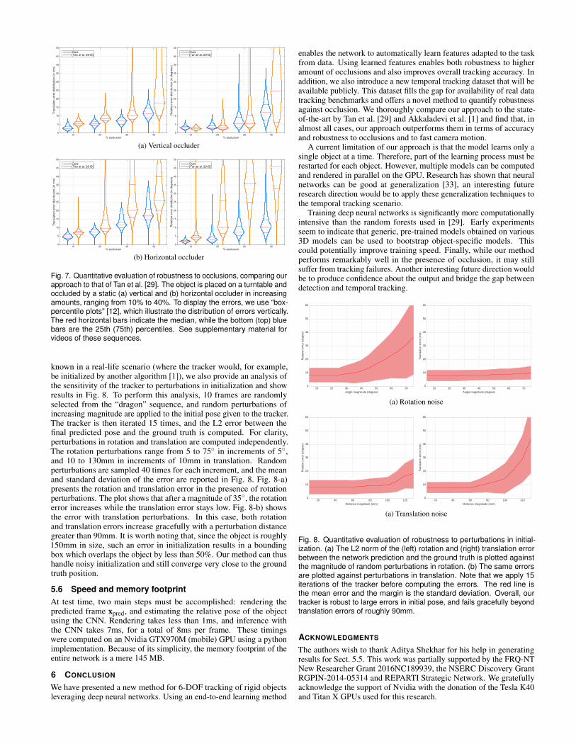
5.4 Robustness to occlusion

We systematically evaluate the robustness of our approach to occlusions,and compare it to Tan et al. [29] on our dataset of controlled occlusioncases. To ensure that each tracker is not artificially penalized formissing a single frame (and thus reporting very high error for thissingle mistake), each tracker is initialized to the ground truth poseevery 15 frames.

Fig. 7 reports the errors on translation and rotation for all occlusionscenarios. Both methods perform similarly when occlusion is 10%.In the 20% case, differences begin to arise: the translation error ofTan et al. begins to increase, most notably in the horizontal occluderscenario. Differences continue to increase with occlusion percentage:

when it reaches 30%, the approach of Tan et al. [29] often loses trackof the object almost immediately, while ours maintains a reasonableestimate. These results are corroborated by example frames fromselected sequences, shown in Fig. 9. The horizontal occluder caseappears to be more difficult for both methods: this is probably dueto the fact that the dragon head and wings represent discriminativefeatures that are helpful for tracking. See the supplementary materialfor all the videos.

5.5 Robustness to initialization

In the experiments presented above, the tracker is always initializedto the ground truth object position. Since that position may not be

% occlusion10 20 30 40

Tra

nsla

tion e

rror

dis

trib

ution (

in m

m)

0

5

10

15

20

25

30

35

40

45

50

Ours[Tan et al. 2015]

% occlusion10 20 30 40

Rota

tion e

rror

dis

trib

ution (

in d

egre

es)

0

5

10

15

20

25

30

35

40

45

50

Ours[Tan et al. 2015]

(a) Vertical occluder

% occlusion10 20 30 40

Tra

nsla

tion e

rror

dis

trib

ution (

in m

m)

0

5

10

15

20

25

30

35

40

45

50

Ours[Tan et al. 2015]

% occlusion10 20 30 40

Rota

tion e

rror

dis

trib

ution (

in d

egre

es)

0

5

10

15

20

25

30

35

40

45

50

Ours[Tan et al. 2015]

(b) Horizontal occluder

Fig. 7. Quantitative evaluation of robustness to occlusions, comparing ourapproach to that of Tan et al. [29]. The object is placed on a turntable andoccluded by a static (a) vertical and (b) horizontal occluder in increasingamounts, ranging from 10% to 40%. To display the errors, we use “box-percentile plots” [12], which illustrate the distribution of errors vertically.The red horizontal bars indicate the median, while the bottom (top) bluebars are the 25th (75th) percentiles. See supplementary material forvideos of these sequences.

known in a real-life scenario (where the tracker would, for example,be initialized by another algorithm [1]), we also provide an analysis ofthe sensitivity of the tracker to perturbations in initialization and showresults in Fig. 8. To perform this analysis, 10 frames are randomlyselected from the “dragon” sequence, and random perturbations ofincreasing magnitude are applied to the initial pose given to the tracker.The tracker is then iterated 15 times, and the L2 error between thefinal predicted pose and the ground truth is computed. For clarity,perturbations in rotation and translation are computed independently.The rotation perturbations range from 5 to 75◦ in increments of 5◦,and 10 to 130mm in increments of 10mm in translation. Randomperturbations are sampled 40 times for each increment, and the meanand standard deviation of the error are reported in Fig. 8. Fig. 8-a)presents the rotation and translation error in the presence of rotationperturbations. The plot shows that after a magnitude of 35◦, the rotationerror increases while the translation error stays low. Fig. 8-b) showsthe error with translation perturbations. In this case, both rotationand translation errors increase gracefully with a perturbation distancegreater than 90mm. It is worth noting that, since the object is roughly150mm in size, such an error in initialization results in a boundingbox which overlaps the object by less than 50%. Our method can thushandle noisy initialization and still converge very close to the groundtruth position.

5.6 Speed and memory footprintAt test time, two main steps must be accomplished: rendering thepredicted frame xpred, and estimating the relative pose of the objectusing the CNN. Rendering takes less than 1ms, and inference withthe CNN takes 7ms, for a total of 8ms per frame. These timingswere computed on an Nvidia GTX970M (mobile) GPU using a pythonimplementation. Because of its simplicity, the memory footprint of theentire network is a mere 145 MB.

6 CONCLUSION

We have presented a new method for 6-DOF tracking of rigid objectsleveraging deep neural networks. Using an end-to-end learning method

enables the network to automatically learn features adapted to the taskfrom data. Using learned features enables both robustness to higheramount of occlusions and also improves overall tracking accuracy. Inaddition, we also introduce a new temporal tracking dataset that will beavailable publicly. This dataset fills the gap for availability of real datatracking benchmarks and offers a novel method to quantify robustnessagainst occlusion. We thoroughly compare our approach to the state-of-the-art by Tan et al. [29] and Akkaladevi et al. [1] and find that, inalmost all cases, our approach outperforms them in terms of accuracyand robustness to occlusions and to fast camera motion.

A current limitation of our approach is that the model learns only asingle object at a time. Therefore, part of the learning process must berestarted for each object. However, multiple models can be computedand rendered in parallel on the GPU. Research has shown that neuralnetworks can be good at generalization [33], an interesting futureresearch direction would be to apply these generalization techniques tothe temporal tracking scenario.

Training deep neural networks is significantly more computationallyintensive than the random forests used in [29]. Early experimentsseem to indicate that generic, pre-trained models obtained on various3D models can be used to bootstrap object-specific models. Thiscould potentially improve training speed. Finally, while our methodperforms remarkably well in the presence of occlusion, it may stillsuffer from tracking failures. Another interesting future direction wouldbe to produce confidence about the output and bridge the gap betweendetection and temporal tracking.

10 20 30 40 50 60 70Angle magnitude (degree)

0

10

20

30

40

50

60R

otat

ion 

erro

r (d

egre

e)

10 20 30 40 50 60 70Angle magnitude (degree)

0

10

20

30

40

50

60

Tra

nsla

tion 

erro

r (m

m)

(a) Rotation noise

20 40 60 80 100 120Distance magnitude (mm)

0

10

20

30

40

50

60

Rot

atio

n er

ror 

(deg

ree)

20 40 60 80 100 120Distance magnitude (mm)

0

10

20

30

40

50

60T

rans

latio

n er

ror 

(mm

)

(a) Translation noise

Fig. 8. Quantitative evaluation of robustness to perturbations in initial-ization. (a) The L2 norm of the (left) rotation and (right) translation errorbetween the network prediction and the ground truth is plotted againstthe magnitude of random perturbations in rotation. (b) The same errorsare plotted against perturbations in translation. Note that we apply 15iterations of the tracker before computing the errors. The red line isthe mean error and the margin is the standard deviation. Overall, ourtracker is robust to large errors in initial pose, and fails gracefully beyondtranslation errors of roughly 90mm.

ACKNOWLEDGMENTS

The authors wish to thank Aditya Shekhar for his help in generatingresults for Sect. 5.5. This work was partially supported by the FRQ-NTNew Researcher Grant 2016NC189939, the NSERC Discovery GrantRGPIN-2014-05314 and REPARTI Strategic Network. We gratefullyacknowledge the support of Nvidia with the donation of the Tesla K40and Titan X GPUs used for this research.

20%

occl

usio

n,ou

rs20

%oc

clus

ion,

[29]

40%

occl

usio

n,ou

rs40

%oc

clus

ion,

[29]

(a) t = 0 (initialization) (b) t = 3 (c) t = 6 (d) t = 9 (e) t = 12

Fig. 9. Qualitative evaluation of robustness to occlusions, comparing our approach to that of Tan et al. [29]. Representative examples were chosenfrom the same sequences that were used to generate the plots in Fig. 7. Each column shows the prediction immediately after initialization (t = 0),and t = 3, 6, 9, and 12 frames later. Our method is significantly more robust to occlusion that Tan et al. See supplementary material for videos ofthese sequences.

REFERENCES

[1] S. Akkaladevi, M. Ankerl, C. Heindl, and A. Pichler. Tracking multiplerigid symmetric and non-symmetric objects in real-time using depth data.In IEEE International Conference on Robotics and Automation, pages5644–5649, 2016.

[2] A. Aldoma, F. Tombari, J. Prankl, A. Richtsfeld, L. Di Stefano, andM. Vincze. Multimodal cue integration through hypotheses verification forrgb-d object recognition and 6dof pose estimation. In IEEE InternationalConference on Robotics and Automation, pages 2104–2111, 2013.

[3] L. Bertinetto, J. Valmadre, J. F. Henriques, A. Vedaldi, and P. H. Torr.Fully-convolutional siamese networks for object tracking. In EuropeanConference on Computer Vision, pages 850–865. Springer, 2016.

[4] E. Brachmann, F. Michel, A. Krull, M. Ying Yang, S. Gumhold, et al.Uncertainty-driven 6d pose estimation of objects and scenes from a sin-gle rgb image. In IEEE Conference on Computer Vision and PatternRecognition, pages 3364–3372, 2016.

[5] L. Breiman. Random forests. Machine learning, 45(1):5–32, 2001.[6] N. Brunetto, S. Salti, N. Fioraio, T. Cavallari, and L. Stefano. Fusion of

inertial and visual measurements for rgb-d slam on mobile devices. InIEEE International Conference on Computer Vision Workshops, pages1–9, 2015.

[7] C. Choi and H. I. Christensen. RGB-D object tracking: A particle filterapproach on GPU. IEEE International Conference on Intelligent Robotsand Systems, pages 1084–1091, 2013.

[8] D.-A. Clevert, T. Unterthiner, and S. Hochreiter. Fast and accuratedeep network learning by exponential linear units (elus). arXiv preprintarXiv:1511.07289, 2015.

[9] A. Crivellaro, M. Rad, Y. Verdie, K. Moo Yi, P. Fua, and V. Lepetit. Anovel representation of parts for accurate 3d object detection and tracking

in monocular images. In IEEE International Conference on ComputerVision, pages 4391–4399, 2015.

[10] D. DeTone, T. Malisiewicz, and A. Rabinovich. Deep image homographyestimation. arXiv preprint arXiv:1606.03798, 2016.

[11] A. Doumanoglou, V. Balntas, R. Kouskouridas, and T.-K. Kim. Siameseregression networks with efficient mid-level feature extraction for 3dobject pose estimation. arXiv preprint arXiv:1607.02257, 2016.

[12] W. W. Esty and J. D. Banfield. The box-percentile plot. Journal ofStatistical Software, 8(i17):1–14, 2003.

[13] Q. Gan, Q. Guo, Z. Zhang, and K. Cho. First step toward model-free,anonymous object tracking with recurrent neural networks. arXiv preprintarXiv:1511.06425, 2015.

[14] S. Garrido-Jurado, R. Munoz-Salinas, F. J. Madrid-Cuevas, and M. J.Marın-Jimenez. Automatic generation and detection of highly reliablefiducial markers under occlusion. Pattern Recognition, 47(6):2280–2292,2014.

[15] S. Hinterstoisser, V. Lepetit, S. Ilic, S. Holzer, G. Bradski, K. Konolige,and N. Navab. Model based training, detection and pose estimation oftexture-less 3d objects in heavily cluttered scenes. In Asian conference oncomputer vision, pages 548–562. Springer, 2012.

[16] W. Kehl, F. Milletari, F. Tombari, S. Ilic, and N. Navab. Deep learningof local RGB-D patches for 3D object detection and 6D pose estimation.In European Conference on Computer Vision, pages 205–220. Springer,2016.

[17] A. Kendall, M. Grimes, and R. Cipolla. PoseNet: A convolutional net-work for real-time 6-dof camera relocalization. In IEEE InternationalConference on Computer Vision, pages 2938–2946, 2015.

[18] D. Kingma and J. Ba. Adam: A method for stochastic optimization. InInternational Conference on Learning Representations, pages 1–15, 2015.

[19] A. Krull, E. Brachmann, F. Michel, M. Ying Yang, S. Gumhold, andC. Rother. Learning analysis-by-synthesis for 6d pose estimation in rgb-dimages. In IEEE International Conference on Computer Vision, pages954–962, 2015.

[20] A. Krull, E. Brachmann, S. Nowozin, F. Michel, J. Shotton, and C. Rother.Poseagent: Budget-constrained 6d object pose estimation via reinforce-ment learning. arXiv preprint arXiv:1612.03779, 2016.

[21] A. Krull, F. Michel, E. Brachmann, S. Gumhold, S. Ihrke, and C. Rother.6-dof model based tracking via object coordinate regression. In AsianConference on Computer Vision, pages 384–399, 2014.

[22] J. Kwon, M. Choi, F. C. Park, and C. Chun. Particle filtering on theeuclidean group: framework and applications. Robotica, 25(06):725–737,2007.

[23] R. A. Newcombe, S. Izadi, O. Hilliges, D. Molyneaux, D. Kim, A. J.Davison, P. Kohi, J. Shotton, S. Hodges, and A. Fitzgibbon. Kinectfusion:Real-time dense surface mapping and tracking. In IEEE InternationalSymposium on Mixed and Augmented Reality, pages 127–136. IEEE, 2011.

[24] M. Oberweger, P. Wohlhart, and V. Lepetit. Training a feedback loop forhand pose estimation. In IEEE International Conference on ComputerVision, pages 3316–3324, 2015.

[25] G. Pavlakos, X. Zhou, A. Chan, K. G. Derpanis, and K. Daniilidis. 6-dofobject pose from semantic keypoints. arXiv preprint arXiv:1703.04670,2017.

[26] J. Redmon, S. Divvala, R. Girshick, and A. Farhadi. You only look once:Unified, real-time object detection. In IEEE Conference on ComputerVision and Pattern Recognition, pages 779–788, 2016.

[27] S. Ren, K. He, R. Girshick, and J. Sun. Faster R-CNN: Towards real-timeobject detection with region proposal networks. In Advances in neuralinformation processing systems, pages 91–99, 2015.

[28] D. J. Tan and S. Ilic. Multi-forest tracker: A chameleon in tracking. InIEEE Conference on Computer Vision and Pattern Recognition, pages1202–1209, 2014.

[29] D. J. Tan, F. Tombari, S. Ilic, and N. Navab. A versatile learning-based3d temporal tracker: Scalable, robust, online. In IEEE InternationalConference on Computer Vision, pages 693–701, 2015.

[30] P. Tanskanen, K. Kolev, L. Meier, F. Camposeco, O. Saurer, and M. Polle-feys. Live metric 3d reconstruction on mobile phones. In IEEE Interna-tional Conference on Computer Vision, pages 65–72, 2013.

[31] Z. Wang, A. C. Bovik, H. R. Sheikh, and E. P. Simoncelli. Image quality as-sessment: from error visibility to structural similarity. IEEE Transactionson Image Processing, 13(4):600–612, 2004.

[32] O. Wasenmuller, M. Meyer, and D. Stricker. Corbs: Comprehensive rgb-d benchmark for slam using kinect v2. In IEEE Winter Conference onApplications of Computer Vision (WACV), pages 1–7, 2016.

[33] P. Wohlhart and V. Lepetit. Learning descriptors for object recognitionand 3d pose estimation. In IEEE Conference on Computer Vision andPattern Recognition, pages 3109–3118, 2015.

[34] J. Xiao, A. Owens, and A. Torralba. Sun3d: A database of big spaces re-constructed using sfm and object labels. In IEEE International Conferenceon Computer Vision, pages 1625–1632, 2013.