deductive verification of distributed protocols in first ...padon/oded_padon_phd_thesis.pdfraymond...
TRANSCRIPT

Raymond and Beverly Sackler Faculty of Exact Sciences
The Blavatnik School of Computer Science
Deductive Verification of DistributedProtocols in First-Order Logic
Thesis submitted for the degree of Doctor of Philosophy
by
Oded Padon
This work was carried out under the supervision of
Professor Mooly Sagiv
and the consultation of
Doctor Sharon Shoham
Submitted to the Senate of Tel Aviv University
December 2018

c© 2018
Copyright by Oded Padon
All Rights Reserved

Acknowledgements
I am grateful to all those who contributed to the research presented in this thesis.
First and foremost, to my advisor Mooly Sagiv, and to Sharon Shoham. Their sharp and
insightful guidance, support, encouragement, patience, and enthusiasm have shaped every
step of the way, and were crucial in making the journey both fruitful and enjoyable. It has
been a true privilege to work with Mooly and Sharon.
To Ken McMillan, for the summer I spent as an intern at Microsoft Research and for our
collaboration since. Insightful and brilliant discussions with Ken motivated and inspired
much of the research presented in this thesis.
To Neil Immerman, for our collaboration and for many valuable discussions from which I
learned a lot, and for providing feedback on a draft of this thesis.
To Andreas Podelski, for our collaboration, and for motivating me to work on liveness and
temporal proofs.
To Nikolaj Bjørner, for countless enlightening discussions, and for providing feedback on a
draft of this thesis.
To my collaborators in the papers on which this thesis is based: Jochen Hoenicke, Aleksandr
Karbyshev, Giuliano Losa, and Aurojit Panda.
To the European Research Council and to the Google PhD Fellowship Program for their
generous financial support.
To Gilit Zohar-Oren, for all the administrative help and support, and for always being a
source of sound advice. To Anat Amirav, for her valuable help and willingness to assist.
To my office mates and colleagues in Tel Aviv University’s programming languages group,
for many interesting and supportive discussions, and for useful feedback along the way.
Finally, to my parents Yaniv and Amalia, and to my wife Ella, for her endless support, which
makes it all possible.


Abstract
Distributed algorithms and distributed systems are a critical component of modern
computing infrastructure. However, ensuring that these algorithms and systems are correct
under all operating scenarios is notoriously challenging. Formal verification is a way to
mathematically prove that algorithms and systems are correct by using a computer to
check all scenarios and corner cases, providing a level of certainty that is beyond manual
mathematical proofs. However, applying formal verification to distributed algorithms and
distributed systems is nontrivial, since they usually have infinitely-many states and, in
general, automatically checking their correctness is undecidable.
This thesis explores formal verification of infinite-state systems, and distributed algo-
rithms in particular, using a decidable fragment of first-order logic. The main idea is to
express infinite-state systems, their correctness properties, and their inductive invariants,
in a decidable fragment of first-order logic. Thus, the undecidable verification problem is
essentially decomposed into decidable sub-problems, which can be solved by existing mature
and optimized automated solvers.
Theoretical contributions are developed in several aspects, including the surprising
expressiveness of the decidable fragment considered, the decidability question of the problem
of inductive invariant inference, and the applicability of first-order logic for liveness and
temporal proofs. Based on these ideas, a practical methodology is also developed for
verification of both safety and liveness properties of infinite-state systems. The methodology
is used to verify several challenging distributed algorithms, including variants of the Paxos
algorithm, and several distributed algorithms that are formally verified for the first time.


Contents
1 Introduction 1
1.1 Logic-Based Deductive Verification . . . . . . . . . . . . . . . . . . . . . . . . 1
1.2 Inductive Invariants . . . . . . . . . . . . . . . . . . . . . . . . . . . . . . . . 6
1.3 Liveness and Temporal Verification . . . . . . . . . . . . . . . . . . . . . . . . 8
1.4 Distributed Protocols . . . . . . . . . . . . . . . . . . . . . . . . . . . . . . . 9
1.5 Contributions . . . . . . . . . . . . . . . . . . . . . . . . . . . . . . . . . . . . 11
1.5.1 Modeling in a Decidable Fragment of First-Order Logic . . . . . . . . 11
1.5.2 Decidability of Invariant Inference . . . . . . . . . . . . . . . . . . . . 18
1.5.3 Interactive Inference of Universal Invariants . . . . . . . . . . . . . . . 20
1.5.4 Liveness and Temporal Verification . . . . . . . . . . . . . . . . . . . . 20
1.5.5 Verification of Protocols from the Paxos Family . . . . . . . . . . . . . 23
1.6 How to Read This Thesis . . . . . . . . . . . . . . . . . . . . . . . . . . . . . 26
I Modeling in a Decidable Fragment of First-Order Logic 29
2 Preliminaries 30
2.1 Many-Sorted First-Order Logic . . . . . . . . . . . . . . . . . . . . . . . . . . 30
2.2 Many-Sorted EPR . . . . . . . . . . . . . . . . . . . . . . . . . . . . . . . . . 33
2.2.1 Classical EPR . . . . . . . . . . . . . . . . . . . . . . . . . . . . . . . . 34
2.2.2 Many-Sorted Extension of EPR . . . . . . . . . . . . . . . . . . . . . . 35
2.3 Transition Systems . . . . . . . . . . . . . . . . . . . . . . . . . . . . . . . . . 36
2.4 Transition Systems in First-Order Logic . . . . . . . . . . . . . . . . . . . . . 37
2.4.1 Transition Systems . . . . . . . . . . . . . . . . . . . . . . . . . . . . . 37
2.4.2 Safety Properties and Inductive Invariants . . . . . . . . . . . . . . . . 38
2.4.3 Finite vs. Infinite Structures . . . . . . . . . . . . . . . . . . . . . . . 39
2.5 RML: Relational Modeling Language . . . . . . . . . . . . . . . . . . . . . . . 40
vii

2.5.1 Syntax . . . . . . . . . . . . . . . . . . . . . . . . . . . . . . . . . . . . 40
2.5.2 Axiomatic Semantics . . . . . . . . . . . . . . . . . . . . . . . . . . . . 44
2.5.3 Quantifier Alternation Structure . . . . . . . . . . . . . . . . . . . . . 46
2.5.4 Turing-Completeness . . . . . . . . . . . . . . . . . . . . . . . . . . . . 47
3 Modeling in First-Order Logic 48
3.1 Motivating Examples . . . . . . . . . . . . . . . . . . . . . . . . . . . . . . . . 49
3.1.1 Leader Election in a Ring Protocol . . . . . . . . . . . . . . . . . . . . 49
3.1.2 Majority Vote Protocol . . . . . . . . . . . . . . . . . . . . . . . . . . 52
3.2 Total Orders . . . . . . . . . . . . . . . . . . . . . . . . . . . . . . . . . . . . 54
3.3 Deterministic Paths . . . . . . . . . . . . . . . . . . . . . . . . . . . . . . . . 55
3.3.1 Line . . . . . . . . . . . . . . . . . . . . . . . . . . . . . . . . . . . . . 56
3.3.2 Forest: Acyclic Partial Function . . . . . . . . . . . . . . . . . . . . . 59
3.3.3 Ring . . . . . . . . . . . . . . . . . . . . . . . . . . . . . . . . . . . . . 60
3.3.4 General Partial Function . . . . . . . . . . . . . . . . . . . . . . . . . 62
3.4 Higher-Order Logic and Cardinality Thresholds . . . . . . . . . . . . . . . . . 66
3.4.1 Expressing Higher-Order Logic . . . . . . . . . . . . . . . . . . . . . . 66
3.4.2 Quorums and Cardinality Thresholds . . . . . . . . . . . . . . . . . . 67
3.5 Network Semantics . . . . . . . . . . . . . . . . . . . . . . . . . . . . . . . . . 69
3.5.1 Communication Channel Semantics . . . . . . . . . . . . . . . . . . . 70
3.5.2 Asynchrony and Concurrency . . . . . . . . . . . . . . . . . . . . . . . 72
3.6 Related Work for Chapter 3 . . . . . . . . . . . . . . . . . . . . . . . . . . . . 73
4 Eliminating Quantifier Alternations Cycles: Paxos Made EPR 74
4.1 Methodology for Decidable Verification . . . . . . . . . . . . . . . . . . . . . . 75
4.1.1 Modeling in Uninterpreted First-Order Logic . . . . . . . . . . . . . . 76
4.1.2 Transformation to EPR Using Derived Relations . . . . . . . . . . . . 76
4.1.3 Automatic Generation of Update Code . . . . . . . . . . . . . . . . . . 83
4.2 Introduction to Paxos . . . . . . . . . . . . . . . . . . . . . . . . . . . . . . . 84
4.3 Paxos in First-Order Logic . . . . . . . . . . . . . . . . . . . . . . . . . . . . 87
4.3.1 Protocol Model . . . . . . . . . . . . . . . . . . . . . . . . . . . . . . . 87
4.3.2 Inductive Invariant . . . . . . . . . . . . . . . . . . . . . . . . . . . . . 90
4.4 Paxos in EPR . . . . . . . . . . . . . . . . . . . . . . . . . . . . . . . . . . . . 92
4.4.1 Derived Relation for Left Rounds . . . . . . . . . . . . . . . . . . . . . 93
4.4.2 Derived Relation for Joined Rounds . . . . . . . . . . . . . . . . . . . 93

4.5 Multi-Paxos . . . . . . . . . . . . . . . . . . . . . . . . . . . . . . . . . . . . . 97
4.5.1 Protocol Model in First-Order Logic . . . . . . . . . . . . . . . . . . . 97
4.5.2 Inductive Invariant . . . . . . . . . . . . . . . . . . . . . . . . . . . . . 100
4.5.3 Transformation to EPR . . . . . . . . . . . . . . . . . . . . . . . . . . 101
4.6 Paxos Variants . . . . . . . . . . . . . . . . . . . . . . . . . . . . . . . . . . . 101
4.6.1 Vertical Paxos . . . . . . . . . . . . . . . . . . . . . . . . . . . . . . . 102
4.6.2 Fast Paxos . . . . . . . . . . . . . . . . . . . . . . . . . . . . . . . . . 103
4.6.3 Flexible Paxos . . . . . . . . . . . . . . . . . . . . . . . . . . . . . . . 103
4.6.4 Stoppable Paxos . . . . . . . . . . . . . . . . . . . . . . . . . . . . . . 104
4.7 Evaluation . . . . . . . . . . . . . . . . . . . . . . . . . . . . . . . . . . . . . . 105
4.8 Related Work for Chapter 4 . . . . . . . . . . . . . . . . . . . . . . . . . . . . 107
II Invariant Inference 111
5 Decidability of Invariant Inference 112
5.1 Overview . . . . . . . . . . . . . . . . . . . . . . . . . . . . . . . . . . . . . . 114
5.1.1 Motivation and Background . . . . . . . . . . . . . . . . . . . . . . . . 114
5.1.2 Decidability of Inferring Universal Invariants for Deterministic Paths . 116
5.1.3 Undecidability and Complexity of Invariant Inference . . . . . . . . . 117
5.1.4 Systematic Constructions for Decidability . . . . . . . . . . . . . . . . 117
5.2 The Inductive Invariant Inference Problem . . . . . . . . . . . . . . . . . . . . 119
5.3 Sufficient Conditions for Decidability of INV[C,L] . . . . . . . . . . . . . . . . 121
5.3.1 Quasi-Order and Exclusion Operator for L . . . . . . . . . . . . . . . 122
5.3.2 L-Relaxed Transition System & Decidability of INV[C,L] . . . . . . . . 122
5.4 EPR Classes of Transition Systems and Invariants . . . . . . . . . . . . . . . 125
5.4.1 Classes of Transition Systems and Properties . . . . . . . . . . . . . . 125
5.4.2 Languages of Inductive Invariants . . . . . . . . . . . . . . . . . . . . 126
5.4.3 vL and AvoidL in EPR . . . . . . . . . . . . . . . . . . . . . . . . . . 126
5.5 Decidability of Inferring Universal Invariants for Deterministic Paths . . . . . 128
5.5.1 Transition System Class for Deterministic Paths . . . . . . . . . . . . 129
5.5.2 Deterministic Paths are Well-Quasi-Ordered by v∀∗ . . . . . . . . . . 130
5.6 Systematic Constructions of Decidable Classes . . . . . . . . . . . . . . . . . 135
5.6.1 Basic Extensions . . . . . . . . . . . . . . . . . . . . . . . . . . . . . . 138
5.6.2 Symmetric Lifting . . . . . . . . . . . . . . . . . . . . . . . . . . . . . 141
5.6.3 Adding Occurrences of Arbitrary Relation Symbols . . . . . . . . . . . 143

5.6.4 Putting It All Together: Application to Learning Switch . . . . . . . . 145
5.7 Undecidability and Complexity of INV[C,L] . . . . . . . . . . . . . . . . . . . 145
5.7.1 Reduction from Counter Machines to INV[C,L] . . . . . . . . . . . . . 146
5.7.2 Undecidability of INV[CDP,LAF] . . . . . . . . . . . . . . . . . . . . . . 148
5.7.3 Undecidability of INV[Cr,L∀∗ ] . . . . . . . . . . . . . . . . . . . . . . . 150
5.7.4 Complexity of INV[CDP,L∀∗ ] is Non-Elementary . . . . . . . . . . . . . 153
5.8 Related Work for Chapter 5 . . . . . . . . . . . . . . . . . . . . . . . . . . . . 154
6 Interactive Inference of Universal Invariants 157
6.1 Overview & Illustration . . . . . . . . . . . . . . . . . . . . . . . . . . . . . . 158
6.2 Interactive Methodology for Safety Verification . . . . . . . . . . . . . . . . . 168
6.2.1 Debugging via Symbolic Bounded Verification . . . . . . . . . . . . . . 169
6.2.2 Interactive Search for Universal Inductive Invariants . . . . . . . . . . 170
6.2.3 Obtaining Minimal CTIs . . . . . . . . . . . . . . . . . . . . . . . . . 172
6.2.4 Formalizing Generalizations as Partial Structures . . . . . . . . . . . . 173
6.2.5 Interactive Generalization . . . . . . . . . . . . . . . . . . . . . . . . . 175
6.3 Evaluation & Discussion . . . . . . . . . . . . . . . . . . . . . . . . . . . . . . 177
6.3.1 Protocols . . . . . . . . . . . . . . . . . . . . . . . . . . . . . . . . . . 177
6.3.2 Results & Discussion . . . . . . . . . . . . . . . . . . . . . . . . . . . . 179
6.4 Related Work for Chapter 6 . . . . . . . . . . . . . . . . . . . . . . . . . . . . 182
III Liveness and Temporal Verification 183
7 Reducing Liveness to Safety in First-Order Logic 184
7.1 Overview . . . . . . . . . . . . . . . . . . . . . . . . . . . . . . . . . . . . . . 187
7.1.1 A Running Example . . . . . . . . . . . . . . . . . . . . . . . . . . . . 189
7.1.2 First-Order Temporal Specification . . . . . . . . . . . . . . . . . . . . 189
7.1.3 Reducing Fair Termination to Safety . . . . . . . . . . . . . . . . . . . 191
7.1.4 A Nested Termination Argument . . . . . . . . . . . . . . . . . . . . . 194
7.2 Preliminaries . . . . . . . . . . . . . . . . . . . . . . . . . . . . . . . . . . . . 194
7.2.1 First-Order Linear Temporal Logic (FO-LTL) . . . . . . . . . . . . . . 195
7.2.2 Fair Transition Systems . . . . . . . . . . . . . . . . . . . . . . . . . . 196
7.2.3 Reducing FO-LTL Verification to Fair Termination . . . . . . . . . . . 197
7.3 Reducing Fair Termination to Safety in First-Order Logic . . . . . . . . . . . 198
7.3.1 Parametric Reduction via Dynamic Abstraction . . . . . . . . . . . . . 199

7.3.2 Uniform Reduction in First-Order Logic . . . . . . . . . . . . . . . . . 201
7.3.3 Detailed Illustration for Ticket Protocol . . . . . . . . . . . . . . . . . 205
7.4 Capturing Nested Termination Arguments . . . . . . . . . . . . . . . . . . . . 207
7.4.1 Alternating Bit Protocol . . . . . . . . . . . . . . . . . . . . . . . . . . 208
7.4.2 Inadequacy of the Fair Termination to Safety Reduction for ABP . . . 209
7.4.3 Reduction with Nesting Structure . . . . . . . . . . . . . . . . . . . . 211
7.5 Limitations of Our Reduction in First-Order Logic . . . . . . . . . . . . . . . 213
7.6 Evaluation . . . . . . . . . . . . . . . . . . . . . . . . . . . . . . . . . . . . . . 216
7.6.1 Examples . . . . . . . . . . . . . . . . . . . . . . . . . . . . . . . . . . 216
7.6.2 Discussion of User Experience . . . . . . . . . . . . . . . . . . . . . . . 220
7.7 Related Work for Chapter 7 . . . . . . . . . . . . . . . . . . . . . . . . . . . . 222
8 Temporal Prophecy 226
8.1 Illustrative Example: Ticket with Task Queues . . . . . . . . . . . . . . . . . 228
8.2 Tableau for FO-LTL . . . . . . . . . . . . . . . . . . . . . . . . . . . . . . . . 230
8.3 Liveness-to-Safety Reduction with Temporal Prophecy . . . . . . . . . . . . . 233
8.3.1 Temporal Prophecy Formulas . . . . . . . . . . . . . . . . . . . . . . . 234
8.3.2 Temporal Prophecy Witnesses . . . . . . . . . . . . . . . . . . . . . . 234
8.3.3 Illustration on the Ticket Protocol with Task Queues . . . . . . . . . . 236
8.4 Closure Under First-Order Reasoning . . . . . . . . . . . . . . . . . . . . . . 239
8.5 Implementation & Evaluation . . . . . . . . . . . . . . . . . . . . . . . . . . . 240
8.5.1 Integration in Ivy . . . . . . . . . . . . . . . . . . . . . . . . . . . . . . 240
8.5.2 Examples . . . . . . . . . . . . . . . . . . . . . . . . . . . . . . . . . . 241
8.5.3 Comparison With Chapter 7 . . . . . . . . . . . . . . . . . . . . . . . 245
8.6 Related Work for Chapter 8 . . . . . . . . . . . . . . . . . . . . . . . . . . . . 245
9 Conclusion 249
Bibliography 253
A Paxos Variants 283
A.1 Vertical Paxos . . . . . . . . . . . . . . . . . . . . . . . . . . . . . . . . . . . . 283
A.1.1 Protocol Model in First-Order Logic . . . . . . . . . . . . . . . . . . . 284
A.1.2 Inductive Invariant . . . . . . . . . . . . . . . . . . . . . . . . . . . . . 287
A.1.3 Transformation to EPR . . . . . . . . . . . . . . . . . . . . . . . . . . 290

A.2 Fast Paxos . . . . . . . . . . . . . . . . . . . . . . . . . . . . . . . . . . . . . 291
A.2.1 FOL model of Fast Paxos . . . . . . . . . . . . . . . . . . . . . . . . . 293
A.2.2 Inductive Invariant . . . . . . . . . . . . . . . . . . . . . . . . . . . . . 294
A.2.3 Transformation to EPR . . . . . . . . . . . . . . . . . . . . . . . . . . 297
A.3 Flexible Paxos . . . . . . . . . . . . . . . . . . . . . . . . . . . . . . . . . . . 298
A.4 Stoppable Paxos . . . . . . . . . . . . . . . . . . . . . . . . . . . . . . . . . . 302
A.4.1 Model of the Protocol . . . . . . . . . . . . . . . . . . . . . . . . . . . 304
A.4.2 Inductive Invariant . . . . . . . . . . . . . . . . . . . . . . . . . . . . . 306
A.4.3 Transformation to EPR . . . . . . . . . . . . . . . . . . . . . . . . . . 307

List of Figures
1.1 Suggested routes for reading this thesis according to the reader’s interest . . . 26
2.1 Syntax of many-sorted first-order logic . . . . . . . . . . . . . . . . . . . . . . 31
2.2 Core syntax of RML . . . . . . . . . . . . . . . . . . . . . . . . . . . . . . . . 41
2.3 Syntactic sugars for RML . . . . . . . . . . . . . . . . . . . . . . . . . . . . . 44
2.4 Rules for weakest precondition of RML commands . . . . . . . . . . . . . . . 45
3.1 RML model of the leader election in a ring protocol . . . . . . . . . . . . . . 50
3.6 RML model of the majority vote toy protocol . . . . . . . . . . . . . . . . . . 52
3.10 Encoding of a total order in first-order logic . . . . . . . . . . . . . . . . . . . 54
3.11 Illustration of classes of graphs with outdegree one . . . . . . . . . . . . . . . 55
3.12 Encoding of a line graph in first-order logic . . . . . . . . . . . . . . . . . . . 57
3.15 Encoding of a forest in first-order logic . . . . . . . . . . . . . . . . . . . . . . 59
3.18 Encoding of a ring in first-order logic . . . . . . . . . . . . . . . . . . . . . . . 61
3.21 Encoding of a general graph with outdegree one in first-order logic . . . . . . 63
3.25 Encoding of a network models in first-order logic . . . . . . . . . . . . . . . . 71
4.1 Flowchart of methodology for eliminating quantifier alternation cycles . . . . 77
4.6 RML model of Paxos consensus algorithm . . . . . . . . . . . . . . . . . . . . 88
4.7 Quantifier alternation graph for EPR model of Paxos . . . . . . . . . . . . . . 88
4.8 Changes to the Paxos model that allow verification in EPR . . . . . . . . . . 88
4.20 Counterexample to induction for EPR model of Paxos after the 1st attempt . 94
4.23 RML model of Multi-Paxos . . . . . . . . . . . . . . . . . . . . . . . . . . . . 98
4.28 Performance of VC checking using Ivy and Z3 for Paxos protocols . . . . . . 105
5.1 A simple loop example. . . . . . . . . . . . . . . . . . . . . . . . . . . . . . . 114
5.22 Infinite sequence of incomparable structures (antichain) w.r.t. v∀∗ . . . . . . 130
5.25 The transformation between STRUCT[Σ,Γ�] and T (X) . . . . . . . . . . . . 132
5.26 RML model of the learning switch network routing algorithm . . . . . . . . . 136
xiii

5.31 Infinite sequence of incomparable models w.r.t. v�1,�2
∀∗ . . . . . . . . . . . . . 139
5.49 Encodings used in the reduction from counter machines . . . . . . . . . . . . 149
6.1 Graphical representation of protocol states . . . . . . . . . . . . . . . . . . . . 159
6.2 Flowchart of bounded verification. . . . . . . . . . . . . . . . . . . . . . . . . 159
6.3 Error trace found by BMC . . . . . . . . . . . . . . . . . . . . . . . . . . . . . 161
6.4 Flowchart of the interactive search for an inductive invariant. . . . . . . . . . 162
6.5 The conjectures found using Ivy for the leader election protocol . . . . . . . . 164
6.6 The 1st CTI generalization step for the leader protocol . . . . . . . . . . . . . 165
6.7 The 2nd CTI generalization step for the leader protocol . . . . . . . . . . . . 166
6.8 The 3rd CTI generalization step for the leader protocol . . . . . . . . . . . . 167
6.15 Evaluation of interactive search for universal invariants . . . . . . . . . . . . . 180
7.1 Temporal verification via liveness-to-safety reduction in first-order logic . . . 188
7.2 Ticket protocol for mutual exclusion . . . . . . . . . . . . . . . . . . . . . . . 189
7.3 Temporal specification of the ticket protocol . . . . . . . . . . . . . . . . . . . 190
7.4 First-order logic specification of the ticket protocol . . . . . . . . . . . . . . . 196
7.5 Monitor that checks the (α, µ)-acyclicity condition . . . . . . . . . . . . . . . 198
7.15 Realization in first-order logic of commands from Figure 7.5 . . . . . . . . . . 204
7.16 Alternating Bit Protocol . . . . . . . . . . . . . . . . . . . . . . . . . . . . . . 208
7.21 Monitor that checks the (η, α, µ)-acyclicity condition . . . . . . . . . . . . . . 212
7.22 Programs demonstrating the limits of our reduction . . . . . . . . . . . . . . 214
7.23 Evaluation of liveness proofs . . . . . . . . . . . . . . . . . . . . . . . . . . . . 217
8.1 Ticket protocol with task queues . . . . . . . . . . . . . . . . . . . . . . . . . 228
8.14 Protocols for which we verified liveness using temporal prophecy . . . . . . . 242
A.1 RML model of Vertical Paxos . . . . . . . . . . . . . . . . . . . . . . . . . . . 285
A.22 RML model of Vertical Paxos in EPR . . . . . . . . . . . . . . . . . . . . . . 292
A.47 RML model of Fast Paxos . . . . . . . . . . . . . . . . . . . . . . . . . . . . . 299
A.48 RML model of Fast Paxos in EPR . . . . . . . . . . . . . . . . . . . . . . . . 300
A.49 RML model of Flexible Paxos . . . . . . . . . . . . . . . . . . . . . . . . . . . 301
A.51 RML model of Stoppable Paxos . . . . . . . . . . . . . . . . . . . . . . . . . . 305
Chapter 1
Introduction
Program verification is one of the fundamental problems of computer science. In program
verification one seeks to prove, with mathematical certainty, that a program (or more
generally computer system), behaves correctly, with respect to a given specification. Turing
already addressed this issue in 1949 [175, 225], suggesting essentially what is now known as
deductive verification, or Floyd-Hoare style verification, as it was developed in the seminal
works of Floyd [80] and Hoare [105]. In Floyd-Hoare style verification, a program is
annotated with local assertions that should imply global correctness. To cite Turing’s 1949
paper “Checking a large routine” [225]:
How can one check a routine in the sense of making sure that it is right? In
order that the man who checks may not have too difficult a task the programmer
should make a number of definite assertions which can be checked individually,
and from which the correctness of the whole programme easily follows.
1.1 Logic-Based Deductive Verification
In deductive verification [161], assertions are expressed as formulas in a logical formalism
and refer to the program’s state. For example, the assertion x > 0 means that the value of
the program variable x is positive. Program statements are also given a logical meaning,
either using Dijkstra’s weakest precondition calculus [66], or alternatively using a two
vocabulary transition formula expressing state transitions. For example, the program
statement x := x + 1 corresponds to the transition formula x′ = x+ 1, where x (resp. x′)
denotes the value of the program variable x before (resp. after) executing the statement.
A Hoare triple, {P } C {Q }, states that if command C is executed in a state satis-
fying assertion P , then its final states satisfy assertion Q. For example, the Hoare triple
1
2 CHAPTER 1. INTRODUCTION
{x ≥ 0 } x := x + 1 {x > 0 } is valid. A program annotated with assertions naturally de-
fines a collection of Hoare triples, which are meant to be valid. Validity of Hoare triples can
be reduced to validity of logical formulas, using the logical meaning of program statements.
For the example, validity of the aforementioned Hoare triple reduces to validity of the formula
(x ≥ 0 ∧ x′ = x+ 1) → x′ > 0. Therefore, once a program is annotated with assertions,
the problem of checking these assertions can be mechanically translated to the problem of
checking validity of logical formulas, called verification conditions. Establishing validity of
logical formulas is also amenable to mechanization, using (interactive or automated) theorem
provers. This approach has become known as deductive program verification, and its end
result is a mechanized proof that a given program is correct. Since the proof is mechanized,
it can be trusted with a higher degree than a manual “paper proof”.
The problem of establishing validity of logical verification conditions (VCs) remains
computationally hard. The difficulty of this problem depends on the logical formalism used
to express assertions and VCs. For software systems, the assertions needed to prove the
program commonly use a rich logical formalism that includes quantifiers, arithmetic, sets,
cardinalities, transitive closure, and more. As a result, checking validity of VCs is usually
undecidable, and in most cases not even recursively enumerable (i.e., no complete proof
system exists). In the verification community, this situation is coped with using two ways
(and their combination): 1. Interactive theorem proving, where the proof is done manually
and the computer merely checks proof steps; and 2. Automated theorem proving, where
heuristics are employed to attempt to automatically solve an undecidable problem.
Interactive theorem proving Interactive theorem provers, also known as proof assistants,
usually support a very rich logical formalism based on dependent type theory or high-order
logic, which can express most of mathematics. Examples include ACL2 [117], Agda [33],
Coq [26], HOL [92] Isabelle [181], Lean [63], PVS [184], and more. While these tools support a
very expressive logical formalism, they usually require great manual effort. Proof construction
is based on the user interactively applying tactics, reducing the current proof goal to simpler
goals, and applying previously proven lemmas and theorems. This essentially requires the
user to provide a very detailed proof, while the tool ensures soundness.
The result is that practical verification of computer systems is very tedious and demands
tremendous manual effort. For example, the seL4 [119] project developed a verified operating
system micro-kernel. This project involves a 20 person-year effort. The code base comprises
of about 10,000 lines of implementation code, and almost half a million lines of proofs and
specifications using Isabelle/HOL. Closer to the application domain of this thesis is the Verdi

1.1. LOGIC-BASED DEDUCTIVE VERIFICATION 3
project [235, 237], which verified an implementation of Raft [183], a distributed protocol of
the Paxos [135] family considered in this thesis. The Verdi project comprises of 530 lines of
implementation code, and 50,000 lines of specifications and proofs using Coq.
Automated theorem proving Automated theorem provers, and SMT (satisfiability
modulo theories) solvers [23, 62], usually support a logical formalism based on first-order
logic modulo theories. Theories can include variants of arithmetic (integer, real, bit-vector,
linear, non-linear), and theories that allow reasoning about common data structures, such
as arrays, lists, strings, algebraic data types, and more. Examples of SMT solvers include
Z3 [61], Yices [71], CVC4 [22], and more. Some solvers also target pure first-order logic, i.e.,
without theories. Examples include Vampire [207], iProver [123], SPASS [234], and more.
What these tools all share in common is that they attempt to solve an undecidable problem,1
and employ heuristics that are meant to be successful on problem instances that arise in
practice.
Deductive verification tools based on SMT solvers have become very successful in the
programming languages and verification communities. A prominent example is Dafny [148],
which uses Z3 to discharge verification conditions. When using Dafny, the user only needs to
annotate the program with assertions, and proving the resulting verification conditions is
completely automated, potentially making verification easier and more practical compared
to interactive theorem proving. For distributed systems, the IronFleet [100] project has
successfully used Dafny and Z3 to verify an implementation of Multi-Paxos [135], a protocol
also considered in this thesis.
Automated solver instability in deductive verification The use of SMT solvers and
automated theorem provers to automatically discharge VCs significantly reduces the proof
burden of the user. However, it also introduces great instability, since the process becomes
sensitive to the solver’s heuristic. Recent systems verification projects such as IronClad [99],
IronFleet [100], and Komodo [75] (using Dafny) identified the underlying solver’s instability
as a major hurdle to practical deductive verification. If the solver succeeds to validate
the user provided assertions, then the program is shown correct and verification succeeds.
However, minor perturbations, e.g. changes to the random seeds used in solvers’ heuristics,
can unpredictably cause the solver to diverge, in which case verification fails. A quotation
from [75, Section 9.1] illustrates the problem from the developers’ perspective:
1While some of the theories supported by the solvers are decidable when restricted to the quantifier-freefragment, software verification in general and verification of distributed protocols in particular requiresquantifiers, which usually lead to undecidability.

4 CHAPTER 1. INTRODUCTION
The most frustrating recurring problem was proof instability. [...] Even once
fixed, the proof may easily timeout again due to minor perturbations. Worse,
minor changes can trigger timeouts in seemingly unrelated proofs.
The fact that the underlying problem is undecidable also means that there is no theoretical
guarantee that breaking verification into smaller problems (e.g., by splitting the code into
several procedures) would improve the solver’s performance. Worst of all, when the solver is
not able to prove the VCs, the user is left wondering whether the assertions they provided
are incorrect, or the solver is just unable to prove them. In such cases the determined user’s
only choice is to trace and debug the solver’s heuristics and figure out what went wrong, a
task only few users are capable of, and even for them it is tedious and time consuming.
This situation is further aggravated by the incremental and iterative process of software
development. That is to say that verification cannot be a huge one-time effort, and it must
be continuous and maintainable with reasonable effort.
Decidable logic for deductive verification This thesis explores the use of a decidable
fragment of first-order logic for deductive verification. Namely, verification conditions are
discharged using an automated theorem prover, and verification is designed to ensure that
VCs are expressed in a decidable logic for which the solver is a decision procedure. The use
of a decidable fragment of first-order logic brings both theoretical and practical benefits, as
well as challenges that must be addressed.
Theoretically, if verification can be structured such that VCs fall in a decidable fragment,
then the automated solver is guaranteed to terminate with a definite answer to the question
“Are the assertions that annotate the program valid or not?”. The fragment considered in
this thesis also has a finite model property. This means that whenever the annotations are
not valid, there is a finite first-order structure that is a counterexample to the validity of
the annotations. The automated solver can find such a model, which serves as a concrete
counterexample that can be communicated to the user.
Practically, using decidable logics can improve the productivity of the verification process.
For the fragment and applications considered in this thesis, initial experience suggests that
Z3’s instability is all but eliminated. This results in a verification process that is significantly
more productive (and enjoyable), since the user reliably receives feedback from the automated
solver: either confirmation that the assertions are valid, or a concrete counterexample to the
contrary. The concrete counterexamples guide the user towards fixing the annotations and
finding valid assertions, forming a quick loop of progress.

1.1. LOGIC-BASED DEDUCTIVE VERIFICATION 5
In light of the theoretical and practical appeal of decidable logics for verification, many
such logics have been considered by the verification community, from as early as the 1980s.
Examples include Presburger arithmetic and a decidable extension to arrays [218], monadic
second-order logic over strings and trees for reasoning about inductive data structures [102],
the BAPA logic (Boolean Algebra and Presburger Arithmetic) for reasoning about set
cardinalities [131], the array property fragment [35], a decidable fragment of separation
logic [25] and the STRAND [158] logic for reasoning about heap data structures, to name a
few.
Any decidable logic poses some restrictions on what can be expressed, in order to obtain
decidability. Therefore, the main challenge in using a decidable logic for deductive verification
is that of expressiveness. Namely, is the logic powerful enough to capture programs of interest,
and express the assertions required to verify them. Indeed, most decidable logics considered
by the verification community are quite powerful, and include some arithmetic (e.g., addition
but not multiplication), and also some form of (possibly restricted) quantification.
This thesis also employs a decidable logical fragment for deductive verification. However,
unlike most decidable fragments considered by the community before, it is a fragment of
pure, uninterpreted, first-order logic. This is unusual, since even full first-order logic (which
is undecidable, but recursively enumerable) is widely considered too weak for program
verification. Pure first-order logic cannot capture notions that are commonly needed to verify
programs and algorithms. For example, it cannot express arithmetic, graph reachability, or
inductive data structures.
This thesis posits that a decidable fragment of first-order logic is well-suited for verification
of distributed protocols, as uninterpreted relations and functions, as well as quantifiers, can
be used to reason about the multiple nodes or threads, messages, values, and other objects
of distributed systems. Quite surprisingly, this thesis shows that using suitable encodings,
pure first-order logic, and even a decidable fragment thereof, can capture proofs of several
complex distributed protocols. The protocols considered are beyond reach of any other
decidable fragment commonly considered by the verification community in the past.
Therefore, we identify the first challenge that this thesis addresses:
Challenge 1 (Expressiveness). How can a decidable fragment of first-order logic capture
the reasoning needed to verify interesting distributed protocols?

6 CHAPTER 1. INTRODUCTION
1.2 Inductive Invariants
An essential feature of computation is iteration, and its most basic manifestation in pro-
gramming is a loop. The assertion annotation that corresponds to a program loop is of
prime importance in deductive verification. This annotation is known as a loop invariant
or inductive invariant, and it is the most direct application of mathematical induction in
program verification.
A valid loop invariant is an assertion that is true in all states that can occur when the
program enters the loop, and also preserved by the loop body. That is, whenever the loop
body executes in a state satisfying the invariant (and also the loop condition, if any), the
post-state must also satisfy the invariant. Therefore, by induction on the number of loop
iterations, it follows that the inductive invariant is satisfied by all states reachable at the
loop head. For example, x > 0 is an inductive invariant for the loop in the following code
segment:
x := 1
while true:
x := x + 1
This follows from the validity of the following two Hoare triples:
{ true } x := 1 {x > 0 } {x > 0 } x := x + 1 {x > 0 }
A perspective advocated by Naur [178], Floyd [80], Dijkstra [65, 66], and Hoare [105],
and even earlier by Goldstine and von Neumann [91], and Turing [225], is that knowing
the inductive invariant is essential to writing a correct loop, and a correct program. From
this perspective of programming as a mathematical activity, it follows that the programmer
should be able to provide inductive invariants rather easily. For if the programmer does not
know the inductive invariant, how could they hope to write the loop code correctly?
However, as we know today, most programmers do not write programs in the same way
a mathematician proves theorems. Indeed, the requirement that inductive invariants be
preserved by the loop body makes them non-intuitive for most programmers. For example,
x > 0 is not an inductive invariant for the loop in the following code segment:
x := 1
y := 1
while true:

1.2. INDUCTIVE INVARIANTS 7
x := x + y
y := y + 2
Even though x > 0 is satisfied by all states reachable at the loop head, it is not an inductive
invariant, since it is not preserved by the loop body. That is, the Hoare triple
{x > 0 } x := x + y ; y := y + 2 {x > 0 }
is not valid (e.g., consider executing the code starting at program state [x 7→ 1, y 7→ −1]).
One inductive invariant for the above loop is x > 0 ∧ y > 0. This invariant is preserved by
the loop body, and the following Hoare triple representing this is valid:
{x > 0 ∧ y > 0 } x := x + y ; y := y + 2 {x > 0 ∧ y > 0 }
Adding the fact y > 0 to the invariant makes it inductive. This is a special case of a common
situation in mathematics, where one must strengthen the hypothesis for a proof by induction.
Another inductive invariant for the above loop is x = 1 +(y−1
2
)2. This invariant is more
tight, and it also implies x > 0. In fact, this invariant, when combined with y ≥ 0, precisely
captures the reachable states of the loop. However, the VCs that result from this invariant
require non-linear integer arithmetic and are thus harder to check. It is also harder to come
up with this inductive invariant in the first place. As this example illustrates, the most
useful inductive invariant is not necessarily the most precise, and useful inductive invariants
often abstract many details of the actual set of reachable states. However, they must still
imply the property we are trying to prove, and of course be preserved by the loop body.
Another difficulty involved with inductive invariants is that they are hard to maintain
as part of the development process. Indeed, a small change to the body of a loop (e.g., for
the purpose of optimization or adding a new feature) could lead to a drastic change in the
required inductive invariant.
As verification requires inductive invariants, and as they are very tricky for programmers
to provide, the verification community has devoted great effort to developing methods for
automatic discovery of inductive invariants.
A continuous and fruitful effort in this direction evolved from Cousot and Cousot’s
Abstract Interpretation [56, 57]. Static analysis by abstract interpretation provides a
multitude of techniques used to analyze software in various domains. Simple abstract
interpretation techniques are employed by standard compilers, and more advanced abstract
interpretation techniques are used in particular applications domains (e.g., [58]), and are

8 CHAPTER 1. INTRODUCTION
an active area of research. However, most techniques based on abstract interpretation find
inductive invariants that prove basic and universal correctness properties (e.g., memory
safety, avoiding of division-by-zero), and are usually not sufficient to prove full functional
correctness.
The problem of finding inductive invariants that allow full functional correctness proofs
is fundamental for deductive verification, and is of both theoretical and practical interest. In
the context of this thesis, checking a given inductive invariant is decidable, since it reduces to
checking a VC in a decidable fragment of first-order logic. In this setting, a natural question
is the decidability of the problem of finding an inductive invariant for a given program
and property. Can the class of programs, properties, and potential invariants be restricted
to make this problem decidable as well? This thesis considers this question, and explores
a connection between the modeling in first-order logic and the well established theory of
well-structured transition systems [6, 76] and well-quasi-orders [130].
From a more practical perspective, a natural question is how to exploit the benefits
of decidability of VC checking to develop a practical interactive methodology for finding
inductive invariants. This thesis explores this direction as well, and shows that using the
decidable fragment we can provide more automated help for finding inductive invariants,
even in an interactive, rather than a fully automated setting.
Thus, we identify the second challenge considered in this thesis:
Challenge 2 (Inductive Invariants). How to find inductive invariants for full functional
correctness proofs? Under what conditions is this problem theoretically decidable? How can
it be approached in practice, exploiting the decidable logical fragment?
1.3 Liveness and Temporal Verification
Inductive invariants can be used to prove safety properties, but they do not suffice to
prove termination, or more generally liveness properties. The distinction between safety
and liveness was introduced by Lamport [134]. Informally, a safety property asserts that
something bad does not happen during system execution. A liveness property asserts that
something good eventually does happen. A particular case of a liveness property is program
termination. However, the notion is more general. Some programs and systems are not
meant to terminate, but to run indefinitely and interact with their environment (e.g., a server
that serves requests, an operating system). Such systems are known as reactive systems [163],
and some of their most important correctness requirements are liveness properties. For

1.4. DISTRIBUTED PROTOCOLS 9
example, a typical liveness property for a reactive system assets that “every request is
eventually followed by a response”. In concurrent and distributed systems, it is typical
for liveness properties to depend on fairness assumptions, such as fair thread scheduling,
eventual message delivery by the network, etc.
A violation of a safety property is a finite execution trace (showing something bad can
happen), while a violation of a liveness property is an infinite execution trace (showing an
infinite execution where something good never happens). This gives the safety vs. liveness
distinction an elegant topological interpretation, such that every property of execution traces
can be expressed as the intersection of a safety property and a liveness property [15].
The canonical way to prove termination and other liveness properties is to use a ranking
function (variant function) into a well-ordered set2 (this dates back to [80, 225]). For example,
to prove termination of a loop, one can provide a function to the natural numbers that
decreases with each loop iteration. For more general liveness properties, the ranking functions
must decrease until the “good thing” happens.
Given a program annotated with a ranking function, a suitable verification condition
can be generated that is valid if and only if the ranking function is decreasing as it should.
However, since the range of the ranking function is a well-ordered set, the logical formalism
used to express the VC must contain a domain that represents the well-ordered set. The most
common examples for ranking functions are functions whose range is the natural numbers (the
ordinal ω), or lexicographic ranking functions with natural components (essentially functions
to ωn). This presents a challenge to verification with first-order logic, since first-order logic
cannot capture the natural numbers, or the notion of a well-founded relation. We therefore
identify the third challenge addressed in this thesis:
Challenge 3 (Liveness). How can a proof technique based on first-order logic, and a decidable
fragment thereof, be used to verify liveness and temporal properties? How can the fact that
first-order logic cannot express well-founded relations be circumvented?
1.4 Distributed Protocols
The main application domain considered in this thesis is verification of distributed protocols.
Distributed protocols (or distributed algorithms) allow a set of discrete computing units
that communicate with each other (e.g., by message passing or shared memory) to achieve
a common task [16]. Distributed protocols are increasingly important, as they are used in
2A set equipped with a well-founded relation is also sufficient.
10 CHAPTER 1. INTRODUCTION
many computer systems, both for performance and for fault tolerance reasons. Distributed
protocols are used in a variety of scales: from multiple computing cores on the same chip, to
global scale cloud infrastructures employed by companies such as Google [37], Amazon [180],
and more.
In addition to their importance, distributed protocols are notoriously hard to design,
implement, test, debug, and formally verify. Indeed, distributed protocols are often hard to
understand even when they appear simple. One reason for this is that a distributed protocol
must function correctly under any behavior of the communication network, relative speeds of
processors, and possible failures. This concurrency and asynchrony introduces a great deal
of non-determinism, in the form of various interleavings of events. For example, messages
can be dropped, delayed, reordered, and duplicated by the network. Further complication
is introduced by the possibility of process failures, either benign (i.e., processes can crash)
or Byzantine (i.e, processes can act arbitrarily, including maliciously). This leads to a
potentially large number of corner cases, and a correct algorithm must handle all of them,
including their combinations.
Another implication is that bugs can occur on rare scenarios, making both testing and
debugging extremely difficult. Testing often cannot be made exhaustive, and a bug may
occur in production due to a rare combination of failures and interleaving of asynchronous
events. In this case, the bug would also be very difficult to reproduce and diagnose. This
makes formal verification of distributed protocols very appealing, as a formal proof ensures
the correctness under all scenarios.
Two anecdotal stories from recent years illustrate the difficulty of designing distributed
protocols and reasoning about their correctness informally:
1. The Chord protocol operates a peer-to-peer distributed hash table [216]. Since its
publication in 2001, Chord had great impact on the distributed computing and systems
community, and in 2011 it won the ACM SIGCOMM Test of Time Paper Award. The
original paper claimed a correctness proof, and a further publication in PODC [154]
presented a more detailed correctness proof. In spite of the original claims, a 2012
paper by Pamela Zave, followed by a series of works [239, 241, 242], shows that the
originally claimed invariants of Chord are incorrect, and that protocol correctness
requires further assumptions and adjustments beyond what is stated in the original
publications.
2. The Zyzzyva protocol for speculative Byzantine fault tolerance was published in SOSP
2007 [125], received a Best Paper Award, and also reported in a CACM article in

1.5. CONTRIBUTIONS 11
2008 [126] and a journal paper in 2009 [127]. The FaB protocol for fast Byzantine fault
tolerance was published in 2005 [166], won the Best Paper Award, and also reported in
a journal paper in 2006 [167]. In 2017, roughly ten years after the original publications,
Ittai Abraham et al. [12] found a safety bug in the Zyzzyva protocol (and demonstrated
it in concrete scenarios), as well as a liveness bug in FaB. Recently they also proposed
a fix to the discovered bugs [13].
These anecdotes demonstrate that informal reasoning about distributed protocols and their
invariants, even by expert researchers and peer-review, is not always sufficient to avoid subtle
bugs and overlooked corner cases.
This thesis focuses on verification of distributed protocols at the protocol (algorithm)
design level, and not at the level of a concrete systems implementation. Protocol designs
are an appealing object for formal verification, since even protocols with rather compact
description (a few pages at most) can have very subtle behaviors, such that informal reasoning
done by humans can take years to uncover subtle bugs. Moreover, uncovering and fixing a
bug at the design level is much easier than later on at the system implementation level.
While not at the focus of this thesis, the results developed in this thesis also open a
path to verification of protocol implementations in distributed systems. This is already
being explored by further graduate students in Tel Aviv University, and promising results of
extending the approach developed in this thesis to systems verification are published in [219].
1.5 Contributions
Below we outline the contributions of this thesis. These contributions were published in [185–
190]. The techniques developed in this thesis are also integrated into the Ivy deductive
verification system [171, 186], which is open-source software and freely available under an
MIT license [169].
1.5.1 Modeling in a Decidable Fragment of First-Order Logic
This thesis develops the use of a decidable fragment of first-order logic for deductive
verification. To achieve this, we must be able to express protocols, properties, and inductive
invariants, in the decidable fragment. We approach this in two steps. First, we consider
expressing protocols, properties, and inductive invariants in first-order logic, which raises
significant challenges. We then consider the restrictions of the decidable fragment, most
importantly restricted use of quantifier alternations, and how to mitigate these restrictions.

12 CHAPTER 1. INTRODUCTION
1.5.1.1 Modeling in First-Order Logic
Our first step is to expressing protocols, properties, and inductive invariants, in first-order
logic. This may seem impossible, since first-order logic cannot even express transitive closure
which is essential to express network topologies (e.g., ring topology), or properties of sets
and cardinalities which are essential for reasoning about distributed consensus protocols.
This was expressed above as Challenge 1, and we outline our approach for addressing it
below. This approach appears in more detail in Chapter 3.
Deterministic paths One of the main hurdles to using first-order logic in verification, is
the fact that it cannot express transitive closure. Several previous works [111–113, 133, 194,
195, 223, 224] showed that reachability for linked data structures such as linked lists and
trees can be encoded in a decidable fragment of first-order logic. This thesis exploits these
ideas to model reachability and transitive closure for verification of distributed protocols.
Modeling reachability in first-order logic can be done for general graphs with outdegree one
(i.e., graphs where the outdegree of every vertex is at most one), with trees and rings as
special cases.
If we represent graphs by a binary relation that captures edges, then we cannot express
graph reachability in first-order logic. The key idea exploited in this thesis is to represent
graphs in a different way, by a path relation. For trees, the path relation is a binary relation
that captures graph reachability, i.e., the transitive closure of the graph edges. From this
relation, graph edges can be expressed using a first-order formula with a single universal
quantifier. It is well known that the successor relation of a total order can be defined in
first-order logic from the order relation: s(x, y) ≡ x < y ∧ ∀z. x < z → y ≤ z, and this is the
idea used to express graph edges from the path relation.
While the path relation is binary for trees (and also forests), for rings and general graphs
we use a ternary relation. For a ring, the transitive closure is trivial (a clique), and does not
contain information about the order of the nodes in the ring. In this setting, the non-trivial
facts about paths in the ring involve three elements. For distinct nodes x, y, z, it may be the
case that y is between x and z in the ring, or that it is not (in which case z is between x and
y). Formally, y is between x and z if y is part of the shortest (i.e., acyclic) path from x to
z. We define the ternary btw relation to capture this fact. For general graphs of outdegree
one, we use a ternary relation that generalizes both the graph reachability relation used for
lines and forests, and the btw used for rings. This ternary relation allows to query, with a
quantifier free formula, whether a node is reachable from another node, whether a node is

1.5. CONTRIBUTIONS 13
part of a cycle, and whether a node is between two other nodes on a cycle.
In the setting considered in this thesis, the modeling in first-order logic is complete,
due to the finite model property of the decidable fragment used. This means that every
counterexample provided by the solver corresponds to an actual graph (with the path relation
interpreted according to actual paths in the graph), and is never spurious. Further details on
the encoding of paths in first-order logic, and its completeness property, appear in Section 3.3.
Quorums and cardinality thresholds Many distributed protocols employ majority sets
or quorums that are defined by thresholds on set cardinalities. For example, a protocol may
wait for at least N2 nodes to confirm a proposal before committing a value, where N is the
total number of nodes. This is often used to ensure consistency. In Byzantine failure models,
where processes can act arbitrarily (including maliciously), a common threshold is 2N3 , where
at most a third of the nodes may be Byzantine. Another common threshold is at least t+ 1
nodes, where at most t node may be faulty.
First-order logic cannot completely capture set cardinalities and thresholds. However,
this thesis exploits the fact that protocol correctness relies on rather simple properties
that are implied by the cardinality threshold, and that these properties can be encoded in
first-order logic. The idea is to use a variant of the standard encoding for second-order logic
in first-order logic (see e.g. [203]). We introduce a sort for quorums, i.e., sets of nodes with
the appropriate cardinality, and use a binary relation member to capture set membership.
Then, properties that are needed for protocol correctness can be axiomatized in first-order
logic.
For example, the fact that any two sets of at least N2 nodes intersect is crucial for many
consensus protocols. This property can be expressed in first order logic:
∀q1, q2 : quorumi. ∃n : node. member(n, q1) ∧member(n, q2)
For Byzantine consensus algorithms that use sets of at least 2N3 nodes, the key property is
that any two quorums intersect at a non-Byzantine node. This can also be expressed in
first-order logic:
∀q1, q2 : quorumii. ∃n : node. ¬byz (n) ∧member(n, q1) ∧member(n, q2)
As a final example, protocols that use sets of t + 1 nodes (when at most t nodes can be
faulty) often rely on the fact that any such set contains at least one non-faulty node. This

14 CHAPTER 1. INTRODUCTION
can also be expressed in first-order logic:
∀q : quorumiii. ∃n : node. ¬byz (n) ∧member(n, q)
This thesis exploits this idea to verify distributed protocols that use a variety of thresholds,
and in all cases we observed the properties that are needed to verify the protocol are actually
expressible in first-order logic. This idea greatly simplifies deductive verification of distributed
protocols, since it cleanly separates out the reasoning about set cardinalities (which is usually
trivial). This allows for a clean formulation of the protocol and its inductive invariants,
as well as the resulting verification conditions, all in first-order logic, greatly simplifying
verification.
Network models Distributed protocols that operate via message passing may assume
any one of a number of network models. One common example is that of a network that
may drop, duplicate, and re-order messages. Another example is a network that may drop
and re-order messages, but may not duplicate them. Another common example is a lossy
FIFO network, in which messages may be dropped, but are otherwise delivered in the order
they were sent. This thesis exploits the fact that all of these network models can be encoded
in first-order logic in a natural way. This facilitates expressing distributed protocols and
their inductive invariants in first-order logic. For example, to represent a FIFO channel, one
uses the axioms for a linear order to capture the order of messages in the channel.
For liveness properties, one usually needs fairness assumptions regarding the network.
Common examples are that every message is eventually delivered, i.e., no dropping; or that
if a message is sent infinitely often then it is eventually delivered, i.e., message dropping is
allowed in a restricted way. The techniques developed in this thesis for liveness and temporal
verification also allow to naturally express such fairness assumptions about the network
model.
1.5.1.2 Eliminating Quantifier Alternation Cycles
This thesis develops the use of a decidable fragment of first-order logic for deductive verifica-
tion. The decidable fragment considered in this thesis is a many-sorted generalization of the
classical Bernays-Schonfinkel-Ramsey class, also called EPR (effectively propositional reason-
ing). The classical (single-sorted) fragment is restricted to relational first-order formulas
(i.e., formulas over a vocabulary that contains constant symbols and relation symbols but no
function symbols) with quantifier prefix ∃∗∀∗ in prenex normal form. Satisfiability of this
1.5. CONTRIBUTIONS 15
fragment is decidable [153, 205]. Moreover, formulas in this fragment enjoy the finite model
property, meaning that a satisfiable formula is guaranteed to have a finite model. Moreover,
it must have a model with no more elements than the sum of the number of constants and
the number of existential quantifiers in the formula.
While the classical single-sorted EPR fragment does not allow any function symbols nor
quantifier alternation except ∃∗∀∗, in a many-sorted setting it can be naturally extended to
allow stratified or acyclic function symbols and quantifier alternation (see e.g., [1, 124]). For
example, a function from sort A to sort B is allowed, but not together with a function from
sort B to sort A. A ∀ ∃ quantifier alternation essentially introduces a (Skolem) function.
This many-sorted EPR extension, henceforward called EPR in this thesis, maintains both
the finite model property and the decidability of the satisfiability problem (albeit increasing
the bound on the model’s size).
The restriction of many-sorted EPR to acyclic functions and quantifier alternations may
seem quite limiting. Indeed, for many protocols considered in this thesis, most notably
Paxos and its variants, a natural encoding in first-order logic results in VCs that contain
quantifier alternation cycles. To mitigate this, this thesis develops a systematic way to
soundly eliminate the cycles, using derived relations and rewrites. These allow the user to
transform the original system such that the resulting system can be verified in EPR, while
the soundness of the transformation itself is also checked using EPR. Thus, a system that
contained quantifier alternation cycles is essentially verified by decomposition into several
problems, each resulting in an EPR check.
Derived relations A useful idea explored in this thesis for eliminating quantifier alterna-
tion cycles is derived relations. The idea is to capture an existential formula by a new relation
symbol, called a derived relation, and then to use the derived relation as a substitute for the
formula, both in the code and in the inductive invariant, thus eliminating some quantifier
alternations. The user is responsible for defining the derived relations and modifying the
code and invariants to use it. It is then possible to automatically check the soundness of
these changes, as well as to generate update code for the derived relation. Note that a
derived relation’s meaning is not exposed to the underlying theorem prover (as it would
result in a quantifier alternation cycle), and its meaning is only manifested in its update
code. This is a form of abstraction, and may lead to spurious counterexamples. However,
if spurious counterexample arise, they are presented to the user, who can address them by
adapting the derived relations’ definitions, or via rewrites as explained below.

16 CHAPTER 1. INTRODUCTION
Rewrites Another useful technique developed in this thesis is to allow the user to soundly
rewrite program conditions. This is useful both to eliminate quantifier alternation cycles,
and to eliminate spurious counterexamples that result from introducing derived relations.
The idea is that if the original model of the protocol contained a formula ϕ (e.g., as the
condition of an if statement), then the user can replace it by another condition ψ, provided
that at that point of the program, ϕ and ψ are equivalent (or in some cases that ϕ implies
ψ). This is useful, since it may be the case that one can prove this holds using EPR, and
then prove the resulting program using EPR, while the proof of the original program cannot
be carried in EPR directly. Effectively, this breaks down a verification problem that contains
quantifier alternation cycles into two problems that are both acyclic.
Transformations using derived relations and rewrites provide a powerful methodology
for verification using EPR that allows to verify a surprisingly wide set of challenging
protocols. Moreover, in the protocols considered in this thesis, the transformations maintain
the simplicity and readability of both the code and the inductive invariants. Another
encouraging fact demonstrated in this thesis is that the transformation can be reusable
across many protocols that share some common structure. This is the case for verification
of several protocols from the Paxos family (outlined further in Section 1.5.5), where the
transformations needed to eliminate quantifier alternation cycles were completely reusable
across protocols.
1.5.1.3 Benefits of Using EPR
One of the key goals for the methodology developed in this thesis is to reach a high level of
productivity in the verification process. This is achieved by a combination of transparency
and stability. Transparency means that whenever verification fails, the user is provided with
a simple and accessible explanation for the failure, and they have a way forward to resolve the
issue. Stability means that the automated solver used in the process is not sensitive to minor
perturbations, e.g., random seeds used by heuristics. As mentioned in Section 1.1, solver
instability has been identified as a major hurdle for practical deductive verification [75, 100].
As an initial evaluation of these ideas, the methodology developed in this thesis is
implemented as part of the Ivy deductive verification system. Ivy uses the Z3 automated
theorem prover for discharging verification conditions in the EPR fragment. As outlined
further in Section 1.5.5, this methodology is evaluated on several challenging distributed
protocols, with promising results. The initial evaluation suggests that using EPR for
verification, as described above, enables to achieve both transparency and stability.

1.5. CONTRIBUTIONS 17
Transparency Transparency means that verification failures are not opaque to the user.
If verification fails, the user should be able to diagnose the failure and apply their creativity
and ingenuity to resolve the issue. In the methodology developed in this thesis, transparency
is maintained at three key points.
First, once an initial model of the protocol is created in first-order logic, Ivy checks if its
verification conditions are in the decidable fragment. If they are not, this failure is reported
to the user in a clear way, by describing the quantifier alternation cycles. The user can
then use derived relations and rewrites, as described above, to eliminate some quantifier
alternations and break the cycles. The modeling language is designed to make the quantifier
structure of the resulting VCs clearly apparent from the program source, facilitating this
process.
Second, when the user applies derived relations and rewrites, their soundness is checked
using EPR queries to Z3. Third, verification of the transformed model is also reduced to
EPR queries (i.e., its resulting verification conditions). The decidability and finite model
property of EPR ensure that if any of the EPR checks fail (either checks for soundness of the
transformations, or for verifying the transformed model), a finite concrete counterexample
will be found by the automated solver. The finite counterexamples are presented to the user,
and guide them towards fixing the problem, thus achieving transparency.
Stability Stability means that the performance of the automated solver used to check
verification conditions is not sensitive to minor perturbations, e.g., random seeds used by
heuristics. The many-sorted EPR decidable fragment used in this thesis is supported by Z3
via model based quantifier instantiation [84]. The experience reported in this thesis shows
that for this fragment, the solver instability of Z3 is all but eliminated.
Across the many challenging verification projects reported in this thesis, Z3 was able
to decide all verification conditions, and most often terminated within a few seconds. This
is the case for both valid VCs, and invalid VCs that arise during the development process.
Even more importantly, the performance was not sensitive to small perturbations or changes
to the random seed used. This results in a verification process that is much more productive
and enjoyable, since the user reliably receives feedback from the automated solver: either
confirmation that the transformations and inductive invariants are valid, or a concrete
counterexample to the contrary. The fact that the solver reliably responds in a few seconds
provides for a quick loop of progress in the verification process, significantly improving
productivity.

18 CHAPTER 1. INTRODUCTION
1.5.2 Decidability of Invariant Inference
When using a decidable fragment for modeling systems and their invariants, checking if an
invariant is inductive is decidable. It is therefore natural to investigate the decidability of the
problem of invariant inference, i.e., the problem of finding a suitable inductive invariant for
proving that a given system satisfies a given safety property. This problem is parameterized by
a language (i.e., infinite set of first-order sentences) L, the search space of potential inductive
invariants. This thesis explores this problem in a general context, develops restrictions
under which this problem is decidable, and also obtains undecidability results that show the
restrictions are necessary.
A key observation is that due to the restriction of the possible inductive invariants to
a given language, the invariant inference problem is different from the safety verification
problem, and hence may be decidable even in cases where safety verification is not. For
invariant inference, the expected outcome is not “safe/unsafe”, but rather “inductive invariant
exists/does not exist in the given language”. Investigating the decidability of this problem is
important to better understand the foundation of existing methods for invariant inference
(e.g., abstract interpretation [56, 57], IC3/PDR [34, 116]), since such methods are only able
to infer inductive invariants in a certain language, so the underlying problem they solve is
actually not safety verification but invariant inference in that language. Therefore, whenever
the invariant inference problem is undecidable, a tool cannot be complete even for the
language in which it is searching; in contrast, when the problem is decidable, tool developers
can aim to have complete algorithms for a restricted language.
This thesis formulates the general problem of inferring inductive invariants in a restricted
language L, applies the technique of well-structured transition systems [5–7, 9, 76] based on
well-quasi-orders (wqo’s) to get sufficient conditions for decidability of invariant inference.
The formalization is parametric in the language L, and associates with each language L a
quasi-order vL on the state space, such that if vL is a wqo, then invariant inference in L is
decidable. This leads to a (parametric) connection between languages in first-order logic
and the theory of decidability of verification based on wqo’s.
This thesis develops the following results for decidability of the invariant inference
problem, which are presented in Chapter 5.
Decidability of universally quantified invariants for deterministic paths This
thesis proves that for programs that manipulate graphs with outdegree one, modeled as
discussed in Section 1.5.1.1, and restricting to universally quantified inductive invariants, the

1.5. CONTRIBUTIONS 19
invariant inference problem is decidable (while safety is still undecidable). This class includes
many programs manipulating singly-linked-lists [112]. The technical proof builds on Kruskal’s
Tree Theorem [129] to show that the suitable vL is a wqo, as it corresponds to homeomorphic
embedding of graphs. Being formulated in logic, this result naturally extends to capture
programs with additional structure beyond graph reachability (e.g., sorting algorithms for
linked lists). The complexity of inferring universally quantified invariants even for linked-list
programs is shown in this thesis to be non-elementary, by reduction from the reachability
problem of lossy counter machines [211, 212].
Undecidability of alternation-free invariants for deterministic paths In the same
setting as above, inferring alternation-free invariants is shown to be undecidable. This
demonstrates that the invariant inference problem is theoretically harder than invariant
checking, since in this setting checking inductiveness of an alternation-free invariant is
decidable. This also shows that mixing universal and existential information even without
alternation makes invariant inference undecidable, so in this setting the restriction to universal
invariants is necessary for decidability of invariant inference.
Undecidability of universally quantified invariants in general If the program is
allowed to manipulate a single unrestricted binary relation, then invariant inference is
undecidable even when restricting to universally quantified invariants. This is shown by
constructing a safe transition system that has a universally quantified inductive invariant if
and only if a given counter machine halts. This shows that the restrictions we develop are
necessary.
Systematic constructions for decidability To overcome the general undecidability
while allowing unrestricted relations, this thesis develops systematic ways to construct classes
of systems and languages for invariants for which invariant inference is decidable. These
constructions start with some established wqo, (e.g. the deterministic paths class with
universal invariants) and gradually extend it to construct new languages with suitable wqo’s.
The constructions utilize the connection between logic and wqo, via the vL definition,
and employ Higman’s Lemma [104] to show that the new languages induces a wqo. Each
construction allows to handle richer system (i.e., in terms of the logical vocabulary), while
decidability is maintained by further restricting the language of potential invariants. The
constructions can be applied iteratively, and this is demonstrated by obtaining a decidable
fragment of the invariant inference problem that captures a nontrivial example of a network

20 CHAPTER 1. INTRODUCTION
learning switch.
1.5.3 Interactive Inference of Universal Invariants
When invariant inference is undecidable, and also when it is decidable and practical techniques
do not (yet) provide full automation, the user must be involved in the process of finding
inductive invariants. Even in such cases, this thesis shows that using a decidable logical
fragment can have further benefits beyond that of providing counterexamples.
Manually finding inductive invariants is one of the most creative and challenging parts
of deductive verification. This was identified above as Challenge 2. For the special case of
universally quantified inductive invariants, this thesis develops an interactive process that
allows the user to incrementally obtain an inductive invariant, where user interaction is
based on a graphical representation of invariants and counterexamples. This methodology is
explained in detail in Chapter 6, and implemented in the Ivy deductive verification system.
The key idea is to check a candidate invariant (which initially could be just the safety
property to be proven), and in case it is not inductive, to graphically present a counterexample
to induction (CTI) to the user, and also allow the user to graphically guide generalization
from the counterexample, which results in modifications to the invariant. This exploits
both a graphical representation of finite structures as graphs (relying on EPR’s finite model
property), and on a graphical representation of universally quantified formulas as excluded
substructures. It also exploits the decidability of EPR to offer further assistance to the
user in the form of well-defined decidable checks that assist in generalization. For example,
checking a potential generalization using bounded unrolling, or minimizing counterexamples
according to user selected criteria. The result of this process is that the user gets much
automated help, but the user is kept in the loop, so the verification process is never stuck
trying to automatically solve an undecidable problem.
1.5.4 Liveness and Temporal Verification
Safety properties can be proven using inductive invariants. In contrast, liveness properties,
and general temporal properties of infinite-state systems are usually proven using ranking
functions or well-founded relations. However, pure first-order logic (without theories) cannot
express the required rankings or the notion of a well-founded relation or well-ordered set.
Therefore, it may seem that liveness verification cannot be done in pure first-order logic, as
identified in Challenge 3. This thesis addresses this challenge and shows that on the contrary,
the formalism of first-order logic provides a unique opportunity for proving liveness, using a

1.5. CONTRIBUTIONS 21
new technique developed in this thesis, and presented in Chapters 7 and 8.
The technique exploits the flexibility of representing states as first-order structures, and
uses first-order temporal logic (FO-LTL) (e.g., [2, 162]) for temporal specification.
This general formalism provides a powerful and natural way to model temporal properties
of infinite-state systems. It naturally supports both unbounded parallelism, where the
system is allowed to dynamically create processes, and infinite-state per process. Unbounded-
parallelism usually requires infinitely many (or quantified) fairness assumptions (e.g., that
every thread is scheduled infinitely often in a program with dynamic thread creation, where
an infinite trace can have infinitely many threads). This is fully supported by the formalism
and the developed proof technique.
The technique developed in this thesis is based on a novel liveness-to-safety reduction3
that transforms temporal verification (expressed in FO-LTL) to safety verification of an
infinite-state system expressed in first-order logic without temporal operators. This allows
us to leverage existing safety verification techniques, and the other techniques developed in
this thesis, to verify liveness and temporal properties. While such a reduction cannot be
complete for computability reasons,4 it is sound, and it was successful in proving liveness of
several challenging protocols, including protocols for which this research obtained the first
mechanized liveness proof.
The liveness-to-safety reduction is based on an abstract notion of acyclicity, using dynamic
abstraction. For finite-state systems, liveness can be proven through acyclicity (the absence
of fair cycles). This is the classical liveness-to-safety reduction of [27]. This also works for
parameterized systems, where the state space is finite (albeit unbounded) for every system
instance [196]. For infinite-state systems, the acyclicity condition is unsound (an infinite-state
system can be acyclic but non-terminating). The liveness-to-safety reduction with dynamic
abstraction defines a finite abstraction that is fine-tuned for each execution trace, while
abstracting only the cycle detection aspect (rather than the actual transitions of the system).
Such fine-tuned abstraction is made possible by exploiting the symbolic representation of the
transition relation in first-order logic, as well as the first-order formulation of the fairness
constraints.
The basic observation used to is that, once a finite domain of objects is fixed, there exist
only finitely many first-order logic structures over the same signature, providing a natural
finite abstraction by projection. The developed technique defines a finite set of objects for
3The term reduction is not used here to mean a complexity theoretic reduction.4The temporal verification problem in this setting is Π1
1-complete [2], while safety verification is in thearithmetical hierarchy.

22 CHAPTER 1. INTRODUCTION
every potential counterexample trace, by further exploiting the first-order representation of
fairness constraints.
This thesis makes the following contributions in the context of liveness and temporal
verification.
Abstract fair cycle parameterized by dynamic abstraction function This thesis
defines a notion of an abstract fair cycle, and this definition is parameterized by a dynamic
finite abstraction function, and a fairness selection function. This definition is general, and
does not depend on the first-order logic formalism. The definition gives rise to a parametric
reduction from liveness (more precisely, from fair termination) to safety that is sound for
systems with both infinitely many states and infinitely many fairness constraints.
Realization in first-Order logic This thesis instantiates the parameterized definition
of an abstract fair cycle in a uniform way for systems expressed in first-order logic and
FO-LTL. The first step uses a tableau construction for FO-LTL to convert any temporal
verification problem into fair termination. Next, the footprint of transitions and abstraction
by projection are used to define a dynamic abstraction function in first-order logic. The
footprint of a transition is the finite set of elements that participated in it. The result
is an automatic transformation from verification of temporal properties to verification of
safety properties. Furthermore, the transformation itself does not introduce any quantifier
alternations, so it maintains the possibility to prove the resulting safety problem using the
EPR decidable fragment, which was indeed used in the protocols considered in this thesis.
Increasing power via a nesting structure To extend the applicability of the reduction,
this thesis defines a nesting structure, which can be specified by the user. This allows to
break the termination argument into several nested levels. In the developed technique, this is
the analogue of a lexicographic termination argument, and we show that it strictly increases
the power of the reduction.
Temporal prophecy and temporal prophecy witnesses An additional mechanism
developed in this thesis to increase the proof power of the liveness-to-safety reduction is
temporal prophecy and prophecy witnesses, which is presented in Chapter 8. Here, the
idea is to augment the system with additional temporal formulas that are not part of
the specification, and also with additional constant symbols that are essentially Skolem
witnesses for temporal formulas. This is shown to strictly increase the proof power of the
1.5. CONTRIBUTIONS 23
safety-to-liveness reduction, and to subsume the nesting structure in this regard. (However,
it does not preserve the simplicity of a “lexicographic” argument.) Moreover, the class of
temporal properties provable via temporal prophecy and the liveness-to-safety reduction is
closed under first-order reasoning, with cut elimination as a special case.
In addition to increasing the proof power, temporal prophecy witnesses also facilitate
verification of the resulting safety problem using the EPR decidable fragment. By introducing
prophecy witnesses, one can often eliminate quantifier alternations in the resulting verification
conditions. The idea is that a temporal prophecy witness is used to name a particular element
(e.g., the thread that is eventually starved), and then inductive invariants can be specified
for this particular constant, rather than with a quantifier. In several cases considered in this
thesis, this allowed to eliminate quantifier alternation cycles.
Implementation and integration in Ivy The liveness-to-safety reduction with temporal
prophecy has been integrated into the Ivy deductive verification system. In Ivy, temporal
prophecy formulas are derived from an inductive invariant provided by the user (for proving
the safety property induced by the liveness-to-safety reduction), which provides a seamless
way to prove temporal properties.
Evaluation on challenging examples The effectiveness of the approach for liveness
verification is demonstrated on some challenging examples. Some cannot be handled without
a nesting structure or temporal prophecy, and some examples require temporal prophecy
witnesses to allow verification in the EPR decidable fragment. To the best of the author’s
knowledge, this research presented the first mechanized liveness proof for both TLB Shoot-
down [29] and Stoppable Paxos [140]. Interestingly, the liveness of Stoppable Paxos is tricky
enough that Lamport et al. prove it using an informal proof of about 3 pages of rigorous
temporal-logic reasoning [140, Section A.2].
1.5.5 Verification of Protocols from the Paxos Family
The main application domain considered in this thesis is verification of protocols from the
Paxos family. Below we provide some background on Paxos, and later outline the main
contributions of this thesis from the perspective of verification of Paxos protocols.
1.5.5.1 Background on Paxos
On of the most important and widely studied algorithms in distributed computing and
distributed systems is the Paxos [135, 136] algorithm for distributed consensus, and the Paxos
24 CHAPTER 1. INTRODUCTION
family of protocols for state machine replication (SMR), which is the most popular approach
for implementing fault tolerant distributed systems [210]. In distributed consensus, a network
of unreliable processors with unreliable communication try to agree on a single value. In
SMR, a (virtual) centralized sequential state machine is replicated across many nodes,
providing fault tolerance while exposing a simple (centralized and sequential) semantics to
its clients. SMR is implemented by repeatedly solving distributed consensus to agree on
the next command to be executed. Fault tolerant distributed computing, achieved using a
protocol from the Paxos family, underlies many services used daily by billions of people from
companies such as Google, Amazon, and more [37, 41, 180].
Paxos, and similar consensus algorithms such as Viewstamped Replication [182] and
Raft [183], are also widely studied (e.g., [94, 159, 232]) because they contain ideas that are
fundamental for distributed computing in general. These include leader election, major-
ity voting and quorum systems, two-phase commit, ballots (also called views or rounds),
reconfiguration, and more. Note that distributed consensus is not solvable in a general
asynchronous setting with failures [77]. However, solutions that provide consistency (i.e.,
processors cannot decide on different values) under all scenarios, and ensure progress under
“good conditions” [96] are possible, and protocols in the Paxos family achieve this.
The Paxos family includes many variants that support various optimizations and features,
and employ different trade-offs. Examples include optimizations that reduce the number
of messages or nodes needed to commit a new command in certain scenarios (e.g., Fast
Paxos [138], Flexible Paxos [107]); reconfiguration, a feature that allows to change the set of
operating nodes while the state-machine is running (e.g., Vertical Paxos [141], Stoppable
Paxos [140]); and more.
Due to its importance, verification of distributed protocols of the Paxos family, and
systems that implement them, is an ongoing research challenge. The systems and program-
ming languages communities have had several recent success stories in verifying Paxos-like
protocols and their implementations in projects such as IronFleet [100], Verdi [235], and
PSync [70].
1.5.5.2 Contributions
This thesis applies deductive verification using first-order logic and EPR to several protocols
in the Paxos family. Quite surprisingly, this thesis shows that protocols as complex as Paxos
can indeed be verified in a decidable fragment, and it presented the first verification of
Paxos in a decidable fragment. For some of the variants, namely Vertical Paxos, Fast Paxos,
1.5. CONTRIBUTIONS 25
and Stoppable Paxos, this thesis presents the first mechanized verification. In this context,
perhaps the greatest feat of this thesis is verification of both safety and liveness of Stoppable
Paxos [140]. Stoppable Paxos is arguably the most intricate algorithm in the Paxos family:
as acknowledged by Lamport et al., “getting the details right was not easy” [140, Section 1].
Their paper includes 10 pages of rigorous informal proof of safety, and 3 additional pages of a
liveness proof composed of rigorous temporal reasoning. Before this thesis, this protocol has
never been formally verified, and state-of-the-art verification projects for simpler variants of
Paxos (e.g, Multi-Paxos, Raft) take between 5,000 and 50,000 lines of proof [40, 100, 235].
In contrast, the models developed in this thesis are a few hundred lines, with a few dozens
of simple invariants that are automatically checked in a decidable logic.
The techniques developed in this thesis have also enabled a recent work [219] that
considers verification of systems implementations (versus protocol design). This work, which
is outside the scope of this thesis, also successfully applies the techniques developed in this
thesis to verify the Raft protocol.
For the protocols in the Paxos family considered here, this thesis makes the following
contributions.
Formalization in first-order logic of protocols and inductive invariants For each
protocol in the Paxos family considered, the techniques of modeling in first-order logic
outlined in Section 1.5.1.1 are employed to model both the protocol and its inductive
invariant in first-order logic.
Transformation to EPR and decidable safety verification For the Paxos protocols
considered, the model in first-order results in verification conditions that contain cyclic
quantifier alternations. This thesis applies the techniques outlined in Section 1.5.1.2 to
eliminate the cycles and enable verification in the decidable EPR fragment. The result is
the first verification of Paxos (in the full asynchronous setting) using a decidable fragment.
Another encouraging observation is that the transformations needed to eliminate the cycles
were completely reusable across all protocols considered, despite significant different features
and optimizations in each protocol. This demonstrates the flexibility and reusability of the
transformation mechanism developed in this thesis.
Liveness verification For several protocols, including the most challenging Stoppable
Paxos, this thesis also applies the temporal verification technique outlines in Section 1.3
to verify liveness. As mentioned above, liveness of Paxos is not guaranteed under general

26 CHAPTER 1. INTRODUCTION
Chapter 2Preliminaries
Chapter 3Modeling inFirst-Order Logic
Chapter 5Decidability of InferringInductive Invariants
Chapter 4Eliminating Quantifier Altern-ation Cycles: Paxos Made EPR
Appendix APaxos Variants
Chapter 6Interactive Inferenceof Universal Invariants
Chapter 7Reducing Liveness toSafety in First-Order Logic
Chapter 8Temporal Prophecy
Distributed Protocols
Logic and Theory
Invariant Inference
Liveness Verification
Figure 1.1: Suggested routes for reading this thesis according to the reader’s interest. Fourroutes are depicted: for readers interested in verification of distributed protocols and Paxosprotocols, for readers interested in logic and theoretical aspects, for readers interested inautomatic or semi-automatic inference of inductive invariants, and for readers interested inliveness and temporal verification. The scenic route going through all chapters in order isnot depicted but is nonetheless suggested.
conditions. This thesis proves the liveness property formalized in [140, Section 4]. Namely,
that the protocol makes progress if eventually there is a unique leader for a high enough ballot
number that is non-faulty and can communicate with a non-faulty quorum. This property is
expressible in FO-LTL, and the fact that the temporal verification technique developed in
this thesis could handle the liveness proof of a protocol as challenging as Stoppable Paxos
demonstrates its applicability.
1.6 How to Read This Thesis
This thesis is organized in three parts, corresponding to the three challenges identified above.
Part I addresses the challenge of modeling protocols in a decidable fragment of first-order logic
(challenge 1). Part II addresses the challenge of finding inductive invariants (challenge 2).
Part III addresses verification of liveness and temporal properties using first-order logic
(challenge 3).
As this thesis contains contributions and raises future research directions on several
topics, different readers could be interested in different contributions and ideas, and need
not read the thesis in its entirety. Below are a few suggested routes for readers with different
interests, along with suggested future research directions. Figure 1.1 depicts the various
suggested routes for reading this thesis (the route going through all chapters in order is
omitted, but is nonetheless suggested).

1.6. HOW TO READ THIS THESIS 27
Reader interested in verification of distributed protocols and Paxos protocols
Skim Chapters 2 and 3 for the formalism of using first-order logic to model protocols. Read
Chapter 4 for safety verification of Paxos and Multi-Paxos, and Appendix A for verification of
Vertical Paxos, Fast Paxos, Flexible Paxos and Stoppable Paxos. Read Chapters 7 and 8 for
liveness verification. Check out the open-source Ivy deductive verification system [169], and
the work of [219] that builds on the ideas of this thesis and extends them to verify executable
implementations for Multi-Paxos and Raft. Try to use Ivy to verify your distributed protocol
or distributed system.
Reader interested in logic and theoretical aspects Read Chapters 2 and 3 for the
formalism of using first-order logic to model infinite-state transition systems. Read Chapter 5
for results on decidability of invariant inference and the connection to well-quasi-orders.
Read Chapters 7 and 8 for an interesting technique to verify liveness properties in first-order
logic, without using ranking functions or well-founded relations. Perhaps ask yourself how
to extend the completeness-for-finite-models results of Section 3.3 to paths in other classes
of graphs, or other properties that are seemingly beyond first-order logic. Ask yourself how
to extend the decidability results of Chapter 5 using other well-quasi-orders, or extend them
to other classes of invariants other than universal, or come up with further restrictions that
also reduce the complexity of invariant inference. Think about the technique developed
in Chapters 7 and 8 as a proof system for first-order linear temporal logic (FO-LTL), and
its connection to well-known systems of arithmetic such as Primitive Recursive Arithmetic
or Peano Arithmetic. The proof system of Chapter 7 cannot prove termination of the
Ackermann function (Section 7.5), and when extended with temporal prophecy it admits a
robust closure property and a cut-elimination theorem (Section 8.4).
Reader interested in automatic or semi-automatic invariant inference Skim
Chapters 2 and 3 for the formalism of using first-order logic to model infinite-state transition
systems. Read Chapter 5 for results on decidability of automatic invariant inference, and
Chapter 6 for a semi-automatic methodology for finding inductive invariants via interactive
generalization. Perhaps think about exploiting the decidable classes of Chapter 5 to create
practical algorithms for invariant inference. Think about ways to improve the technique
of Chapter 6 and make it more automated, or perhaps generalize the idea of interactive
generalization to classes of invariants other than universally quantified. If you are developing
an invariant inference technique, mine this thesis for challenging benchmarks.
28 CHAPTER 1. INTRODUCTION
Reader interested in liveness and temporal verification Read Chapter 2 and op-
tionally skim Chapter 3 for the formalism of using first-order logic to model infinite-state
transition systems. Read Chapter 7 for a technique to verify liveness properties using
an abstract acyclicity test and dynamic abstraction, without using ranking functions or
well-founded relations. Think about the parametric definition of dynamic abstraction and
the abstract acyclicity test (Section 7.3.1), and perhaps apply it in other contexts that are
not based on first-order logic. Read Chapter 8 and think about applying the idea of temporal
prophecy in other contexts not based on first-order logic. Or try to apply your favorite
temporal verification technique to the challenging examples that motivated the techniques
developed in this thesis (specifically Sections 7.4.1 and 8.1).

Part I
Modeling in a Decidable Fragment
of First-Order Logic
29

Chapter 2
Preliminaries
This chapter presents the formalism used in this thesis for deductive verification of infinite-
state systems by specifying both the system and its invariants in first-order logic. Here we
focus on safety verification, and definitions that are only needed for liveness and temporal
verification are deferred to Chapter 7 (Section 7.2).
2.1 Many-Sorted First-Order Logic
We use standard many-sorted first-order logic with equality [203]. A sorted first-order
vocabulary or signature, denoted Σ, consists of sorted constant symbols, sorted function
symbols, and sorted relation symbols. Functions and relation symbols can have any finite
arity, and constant symbols are considered function symbols of arity zero, also called nullary
function symbols. We sometimes write rk to indicate that r is a relation of arity k. Terms
and formulas are constructed according to the syntax listed in Figure 2.1. We always assume
terms and formulas are well-formed and well-sorted. The set of free variables in a term
or a formula is defined as usual. A term without free variables is called a ground term.
A formula without free variables is called a sentence or a closed formula. We sometimes
write ϕ(x1, . . . , xk) (respectively, t(x1, . . . , xk)) to indicate that x1, . . . , xk are free in ϕ
(respectively, t). We sometimes omit the sorts of variables in case they are either clear or
unimportant.
Given a vocabulary Σ, a structure of Σ is a pair s = (D, I), where D is a sorted domain,
and I is an interpretation. The sorted domain D maps each sort s of Σ to a set D(s),
called the domain or universe of s in s. If all these sets are finite, we say that the domain
D and the structure s are finite. By abuse of notation, we sometimes use D to denote⋃s∈ΣD(s), that is, the union of the universes of all the sorts. The interpretation I maps
30

2.1. MANY-SORTED FIRST-ORDER LOGIC 31
〈t〉 ::= terms
| x : s logical variable x
| c constant symbol c
| f (〈t〉, . . . , 〈t〉) application of function f
| ite (〈ϕ〉, 〈t〉, 〈t〉) if-then-else term
〈ϕ〉 ::= formulas
| r (〈t〉, . . . , 〈t〉) membership in relation r
| 〈t〉 = 〈t〉 equality between terms
| 〈ϕ〉 ∧ 〈ϕ〉 conjunction
| 〈ϕ〉 ∨ 〈ϕ〉 disjunction
| 〈ϕ〉 → 〈ϕ〉 implication
| 〈ϕ〉 ↔ 〈ϕ〉 bi-implication
| ¬〈ϕ〉 negation
| ∀x : s. 〈ϕ〉 universal quantification
| ∃x : s. 〈ϕ〉 existential quantification
Figure 2.1: Syntax of terms and formulas in many-sorted first-order logic.
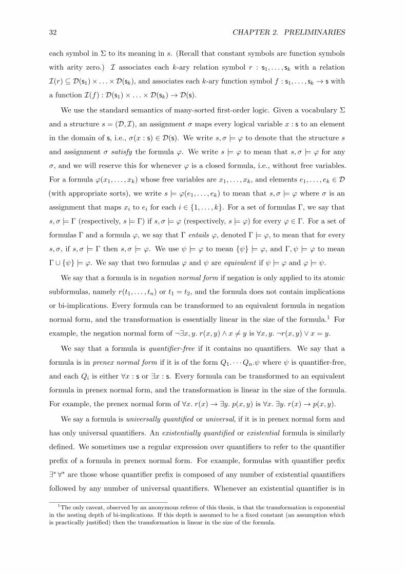
32 CHAPTER 2. PRELIMINARIES
each symbol in Σ to its meaning in s. (Recall that constant symbols are function symbols
with arity zero.) I associates each k-ary relation symbol r : s1, . . . , sk with a relation
I(r) ⊆ D(s1)× . . .×D(sk), and associates each k-ary function symbol f : s1, . . . , sk → s with
a function I(f) : D(s1)× . . .×D(sk)→ D(s).
We use the standard semantics of many-sorted first-order logic. Given a vocabulary Σ
and a structure s = (D, I), an assignment σ maps every logical variable x : s to an element
in the domain of s, i.e., σ(x : s) ∈ D(s). We write s, σ |= ϕ to denote that the structure s
and assignment σ satisfy the formula ϕ. We write s |= ϕ to mean that s, σ |= ϕ for any
σ, and we will reserve this for whenever ϕ is a closed formula, i.e., without free variables.
For a formula ϕ(x1, . . . , xk) whose free variables are x1, . . . , xk, and elements e1, . . . , ek ∈ D(with appropriate sorts), we write s |= ϕ(e1, . . . , ek) to mean that s, σ |= ϕ where σ is an
assignment that maps xi to ei for each i ∈ {1, . . . , k}. For a set of formulas Γ, we say that
s, σ |= Γ (respectively, s |= Γ) if s, σ |= ϕ (respectively, s |= ϕ) for every ϕ ∈ Γ. For a set of
formulas Γ and a formula ϕ, we say that Γ entails ϕ, denoted Γ |= ϕ, to mean that for every
s, σ, if s, σ |= Γ then s, σ |= ϕ. We use ψ |= ϕ to mean {ψ} |= ϕ, and Γ, ψ |= ϕ to mean
Γ ∪ {ψ} |= ϕ. We say that two formulas ϕ and ψ are equivalent if ψ |= ϕ and ϕ |= ψ.
We say that a formula is in negation normal form if negation is only applied to its atomic
subformulas, namely r(t1, . . . , tn) or t1 = t2, and the formula does not contain implications
or bi-implications. Every formula can be transformed to an equivalent formula in negation
normal form, and the transformation is essentially linear in the size of the formula.1 For
example, the negation normal form of ¬∃x, y. r(x, y) ∧ x 6= y is ∀x, y. ¬r(x, y) ∨ x = y.
We say that a formula is quantifier-free if it contains no quantifiers. We say that a
formula is in prenex normal form if it is of the form Q1. · · ·Qn.ψ where ψ is quantifier-free,
and each Qi is either ∀x : s or ∃x : s. Every formula can be transformed to an equivalent
formula in prenex normal form, and the transformation is linear in the size of the formula.
For example, the prenex normal form of ∀x. r(x)→ ∃y. p(x, y) is ∀x. ∃y. r(x)→ p(x, y).
We say a formula is universally quantified or universal, if it is in prenex normal form and
has only universal quantifiers. An existentially quantified or existential formula is similarly
defined. We sometimes use a regular expression over quantifiers to refer to the quantifier
prefix of a formula in prenex normal form. For example, formulas with quantifier prefix
∃∗ ∀∗ are those whose quantifier prefix is composed of any number of existential quantifiers
followed by any number of universal quantifiers. Whenever an existential quantifier is in
1The only caveat, observed by an anonymous referee of this thesis, is that the transformation is exponentialin the nesting depth of bi-implications. If this depth is assumed to be a fixed constant (an assumption whichis practically justified) then the transformation is linear in the size of the formula.

2.2. MANY-SORTED EPR 33
the scope of a universal quantifier or vice versa, we call this a quantifier alternation. A
formula is alternation-free if it contains no quantifier alternations; namely, if it is a Boolean
combination of universal and existential formulas.
We say that a formula ϕ is satisfiable if there are some s and σ such that s, σ |= ϕ.
Otherwise, we say that ϕ is unsatisfiable. We say that a formula ϕ is valid if s, σ |= ϕ for any s
and σ. Note that ϕ is valid if and only if ¬ϕ is unsatisfiable. A formula ϕ(x1, . . . , xn), whose
free variables are x1, . . . , xn, is valid if and only if the closed formula ∀x1, . . . , xn. ϕ(x1, . . . , xn)
is valid; it is satisfiable if and only of the closed formula ∃x1, . . . , xn. ϕ(x1, . . . , xn) is satisfiable.
We say that two formulas ϕ and ψ are equisatisfiable to mean that ϕ is satisfiable if and only
if ψ is satisfiable. Note that if two formulas are equivalent then they are also equisatisfiable,
but the converse does not necessarily hold.
Every formula ϕ can be transformed to an equisatisfiable universal formula, by a process
called Skolemization. The resulting formula is denoted by Sk(ϕ), and the transformation is
essentially linear in the size of ϕ.2 To Skolemize ϕ, we first transform it into negation normal
form, and then eliminate existential quantifiers by using fresh function symbols added to the
vocabulary in the following way. For every existential quantifier ∃y that resides in the scope
of universal quantifiers ∀x1, . . . , ∀xk, remove the existential quantifier ∃y and replace every
occurrence of y (bound by ∃y) by f(x1, . . . , xk), where f is a fresh function symbol added to
the vocabulary. The original formula ϕ and the resulting formula Sk(ϕ) are equisatisfiable.
For example, the Skolemized version of ∀x. r(x) ∨ (∃y. p(x, y) ∧ ∀z. ∃w. q(x, y, z, w)) is
∀x. r(x) ∨ (p(x, fy(x)) ∧ ∀z. q(x, fy(x), z, fw(x, z))), where fy and fz are fresh function
symbols of appropriate arities and sorts. Note that the vocabulary of Sk(ϕ) is a superset of
the vocabulary of ϕ. The added function symbols are referred to as Skolem functions. A
nullary Skolem function, which arises whenever an existential quantifier is not in scope of
any universal quantifier, is called a Skolem constant.
A structure s1 = (D1, I1) (over Σ) is a substructure of a structure s2 = (D2, I2) (over Σ)
if for every sort s ∈ Σ, D1(s) ⊆ D2(s), and for every a ∈ Σ, I1(a) is the restriction of I2(a)
to D1.
2.2 Many-Sorted EPR
This section presents the decidable fragment of first-order logic used in this thesis. We first
review the classical unsorted decidable fragment, and then its straightforward many-sorted
2As Nikolaj Bjørner pointed out, the worst-case is actually quadratic when considering formula sizes asstrings. However, this is not a practical concern, and if it ever may be it can be circumvented by a moreefficient representation.

34 CHAPTER 2. PRELIMINARIES
extension.
2.2.1 Classical EPR
The effectively propositional (EPR) fragment of first-order logic, also known as the Bernays-
Schonfinkel-Ramsey class, is a fragment of first-order logic for which satisfiability is decid-
able [205]. The fragment contains first-order formulas over a relational vocabulary (that is, a
vocabulary that contains constant symbols and relation symbols but no non-nullary function
symbols), where the formula is in prenex normal form and has quantifier prefix ∃∗ ∀∗. The
satisfiability problem for this class is NEXPTIME-complete3 [153]. Beyond decidability, the
EPR fragment has a finite model property, meaning that an EPR formula is satisfiable if
and only if it is satisfiable by a finite structure. The size of this structure is bounded by the
total number of existential quantifiers and constants in the formula.
To see this, consider a formula ϕ = ∃x1, . . . , xn. ∀y1, . . . , ym. ψ, where ψ is quantifier
free, and a structure s = (D, I) such that s |= ϕ. Then, there is an assignment σ such
that s, σ |= ∀y1, . . . , ym. ψ. We can project the structure s to a substructure whose domain
contains only σ(x1), . . . , σ(xn) and I(c1), . . . , I(ck) where c1, . . . , ck are the constants symbols
present in ϕ. This substructure also satisfies ϕ, and its domain is of the required size (and
clearly finite). This projection, and the bound on the size of the model, can also be
understood by considering Skolemized form Sk(ϕ). The existential quantifiers in ϕ result in
Skolem constants, and there are no non-nullary Skolem functions. Thus, the total number
of constants in Sk(ϕ) is precisely the total number of existential quantifiers and constant
symbols in ϕ. The projection described above essentially maintains the interpretation of the
Skolem constants.
The above argument can be seen as a special instance of Herbrand’s theorem, for a case
in which the Herbrand universe is finite. For any universal formula ψ, Herbrand’s theorem
says that ψ is satisfiable if and only if the set of ground instantiations of ψ is satisfiable. For
an EPR formula ϕ, apply Herbrand’s theorem to Sk(ϕ), and observe that the set of ground
instantiations of Sk(ϕ) is finite. This also provides a way to reduce satisfiability of an EPR
formula to propositional SAT, as the satisfiability of a finite set of ground instantiations
amounts to propositional satisfiability.4
3If we fix the maximal arity of relations then satisfiability of EPR formulas is actually in ΣP2 , i.e., second
level of the polynomial-time hierarchy. If we were to further restrict the maximal number of quantifiers usedthen satisfiability is in NP, i.e., the same as satisfiability of propositional formulas.
4We have sidestepped the presence of equality. This is unessential, as we can add the axioms governingthe equality symbol to ϕ, noting that they are universally quantified so ϕ remains in EPR.

2.2. MANY-SORTED EPR 35
2.2.2 Many-Sorted Extension of EPR
While EPR does not allow any (non-nullary) function symbols or quantifier alternation
except ∃∗ ∀∗, in a many-sorted context it can be easily extended to allow stratified function
symbols and quantifier alternations (as formalized below). The extension maintains both
the finite model property and the decidability of the satisfiability problem (see e.g, [1]). The
crux of the idea is to allow functions and quantifier alternations that still ensure that the
vocabulary of the Skolemized formula generates only a finite set of ground terms.
Quantifier alternation graph Let ϕ be a formula in negation normal form over a many-
sorted signature Σ. We define the quantifier alternation graph of ϕ as a directed graph where
the set of vertices is the set of sorts in Σ, and the set of directed edges, called quantifier
alternation edges or ∀ ∃ edges, is defined as follows.
• Function edges: let f be a function that appears in ϕ from sorts s1, . . . , sk to sort s
(i.e., f : s1, . . . , sk → s). Then there is a ∀ ∃ edge from si to s for every i ∈ {1, . . . , k}.
• Quantifier edges: let ∃x : s be an existential quantifier that resides in the scope of
the universal quantifiers ∀x1 : s1, . . . ,∀xk : sk in ϕ. Then there is a ∀ ∃ edge from si to
s for every i ∈ {1, . . . , k}.
Intuitively, quantifier edges are the edges that would arise as function edges from Skolem
functions in Sk(ϕ).
Many-sorted EPR A formula ϕ is stratified if the quantifier alternation graph of its
negation normal form is acyclic. The many-sorted EPR fragment consists of all stratified
formulas. This fragment maintains both the decidability of the satisfiability problem and
the finite model property of unsorted EPR (though the model size bound must be adjusted).
The reason for this is that for a stratified formula ϕ, the vocabulary of Sk(ϕ) generates a
finite set of ground terms (whose size is the adjusted model size bound). Therefore, any
structure that satisfies ϕ can be projected to a finite subset of its domain that still satisfies
ϕ (as in unsorted EPR). Similarly, the set of ground instantiations of Sk(ϕ) is finite, so
the satisfiability problem of many-sorted EPR can be reduced to propositional SAT (as in
unsorted EPR).
In this thesis, whenever we say a formula is (in) EPR, we refer to the many-sorted EPR
fragment.

36 CHAPTER 2. PRELIMINARIES
2.3 Transition Systems
A transition system is a triple T = (S, S0, R), where S is a (possibly infinite) set of states
called the state space, S0 ⊆ S is the set of initial states, and R ⊆ S × S is the transition
relation. A trace of T is a (finite or infinite) sequence of states π = s0, s1, . . ., such that
s0 ∈ S0 and (si, si+1) ∈ R for every 0 ≤ i < |π|. We sometimes denote an infinite trace
by (si)∞i=0, and a finite trace of n transitions by (si)
ni=0. A state s ∈ S is reachable in T
if there exists a finite trace of T , (si)ni=0, such that sn = s. The image of a set A ⊆ S, is
R(A) = {s′ ∈ S | ∃s ∈ A. (s, s′) ∈ R}.
Safety property A safety property is defined by a set P ⊆ S of “good” states.5 A
transition system T satisfies the safety property P , denoted T |= P , if all the reachable
states of T are in P . In this case we say T is safe with respect to P .
Inductive invariant Let T = (S, S0, R) be a transition system and P be a safety property.
A set I ⊆ S is an inductive invariant for (T, P ) if
(i) S0 ⊆ I, that is, all initial states are in I (initiation);
(ii) R(I) ⊆ I, that is, I is closed under the transition relation (consecution); and
(iii) I ⊆ P , that is, all states in I are good (safety).
A well-known observation is that T |= P if and only if there exists an inductive invariant
for (T, P ). The if direction follows since I contains all the reachable states of T , by induction
on the length of traces. For the only if direction, whenever T |= P , the set of all reachable
states of T is an inductive invariant for (T, P ).
Counterexample to induction (CTI) Let T = (S, S0, R) be a transition system and P
be a safety property, and let I ⊆ S be a set of states. A state s ∈ S is a counterexample to
induction (CTI) for I if (i) s ∈ S0 but s 6∈ I, or (ii) s ∈ I, but there exists s′ 6∈ I such that
(s, s′) ∈ R, or (iii) s ∈ I but s 6∈ P . Clearly, a set I ⊆ S is inductive if and only if there is no
counterexample to induction for it.
5This definition of safety as a set of states specializes the more general definition from [15] of safety as aprefix-closed and limit-closed set of traces. However, the difference is not essential for the purposes of thisthesis. In particular, every safety property over traces can be expressed as a safety property over states byaugmenting the states with more information.

2.4. TRANSITION SYSTEMS IN FIRST-ORDER LOGIC 37
2.4 Transition Systems in First-Order Logic
We now provide a formalism for specifying transition systems in first-order logic. We call
such specifications first-order transition systems. We note that this formalism is Turing-
complete (as seen later in Section 2.5.4). Furthermore, Section 2.5 presents a toy imperative
modeling language whose semantics is given by a transition system specified in first-order
logic, and an extended version of this language is supported by the Ivy deductive verification
system [171, 186]. Therefore, users can specify transition systems in first-order logic using
the familiar concept of an imperative programming language.
2.4.1 Transition Systems
Syntax A first-order logic specification of a transition system (S, S0, R) is a tuple
T = (Σ,Γ, ι, τ), where Σ is a first-order vocabulary, Γ is a background theory given as
a finite set6 of closed formulas over Σ, ι is a closed formula over Σ specifying the initial
states, and τ is two-vocabulary closed formula specifying the transition relation. That is, τ
is a closed formula over Σ ] Σ′, where Σ′ = {a′ | a ∈ Σ}.
Semantics A first-order specification (Σ,Γ, ι, τ) defines a class of transition systems, one
for each domain D.7 Let D be any domain (possibly infinite) for Σ, then the transition
system (S, S0, R) defined by (Σ,Γ, ι, τ) is given by:
S = {s = (D, I) | I is an interpretation of Σ for domain D and s |= Γ}
S0 = {s ∈ S | s |= ι}
R ={
(s, s′) ∈ S × S | (s, s′) |= τ}
Thus, in a transition system specified by (Σ,Γ, ι, τ), the states are first-order structures over
vocabulary Σ that satisfy the theory Γ, the initial states are those that satisfy ι, and the
transition relation contains the pairs of states that satisfy the two vocabulary formula τ . In
the above definition, given s = (D, I) ∈ S and s′ = (D, I ′) ∈ S, we use (s, s′) as to denote
the structure (D, I ] I ′′), where I ′′ = λa′ ∈ Σ′. I ′(a). Namely, the structure defined by
(s, s′) is a structure over the vocabulary Σ]Σ′ with the same domain as s and s′, and where
6In this thesis we restrict Γ to be finite. This essentially means we use pure first-order logic, rather thanfirst-order logic modulo a theory, since the conjunction of all formulas in Γ can be expressed as a first-orderformula. The definitions naturally extend to the more general case of Γ as a possibly infinite set of formulas,but this thesis considers only finite first-order theories.
7 While this subtlety is unessential, we note that fixing D outside of the transition system (S, S0, R) isrequired to make S a set of set theory, i.e., without inadvertently defining a set of all sets, as would occur ifwe allow D to be any domain over Σ in the definition of S.
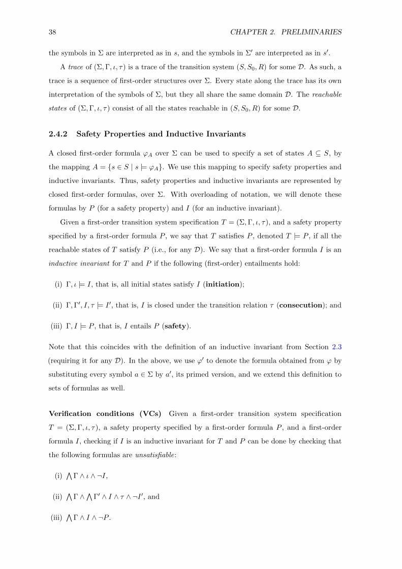
38 CHAPTER 2. PRELIMINARIES
the symbols in Σ are interpreted as in s, and the symbols in Σ′ are interpreted as in s′.
A trace of (Σ,Γ, ι, τ) is a trace of the transition system (S, S0, R) for some D. As such, a
trace is a sequence of first-order structures over Σ. Every state along the trace has its own
interpretation of the symbols of Σ, but they all share the same domain D. The reachable
states of (Σ,Γ, ι, τ) consist of all the states reachable in (S, S0, R) for some D.
2.4.2 Safety Properties and Inductive Invariants
A closed first-order formula ϕA over Σ can be used to specify a set of states A ⊆ S, by
the mapping A = {s ∈ S | s |= ϕA}. We use this mapping to specify safety properties and
inductive invariants. Thus, safety properties and inductive invariants are represented by
closed first-order formulas, over Σ. With overloading of notation, we will denote these
formulas by P (for a safety property) and I (for an inductive invariant).
Given a first-order transition system specification T = (Σ,Γ, ι, τ), and a safety property
specified by a first-order formula P , we say that T satisfies P , denoted T |= P , if all the
reachable states of T satisfy P (i.e., for any D). We say that a first-order formula I is an
inductive invariant for T and P if the following (first-order) entailments hold:
(i) Γ, ι |= I, that is, all initial states satisfy I (initiation);
(ii) Γ,Γ′, I, τ |= I ′, that is, I is closed under the transition relation τ (consecution); and
(iii) Γ, I |= P , that is, I entails P (safety).
Note that this coincides with the definition of an inductive invariant from Section 2.3
(requiring it for any D). In the above, we use ϕ′ to denote the formula obtained from ϕ by
substituting every symbol a ∈ Σ by a′, its primed version, and we extend this definition to
sets of formulas as well.
Verification conditions (VCs) Given a first-order transition system specification
T = (Σ,Γ, ι, τ), a safety property specified by a first-order formula P , and a first-order
formula I, checking if I is an inductive invariant for T and P can be done by checking that
the following formulas are unsatisfiable:
(i)∧
Γ ∧ ι ∧ ¬I,
(ii)∧
Γ ∧∧Γ′ ∧ I ∧ τ ∧ ¬I ′, and
(iii)∧
Γ ∧ I ∧ ¬P .

2.4. TRANSITION SYSTEMS IN FIRST-ORDER LOGIC 39
We refer to these formulas as the verification conditions (VCs) associated with T , P , and I.
In the above, we relied on the fact that Γ is a finite set of first-order formulas, and used∧
Γ
to denote the conjunction of all formulas in Γ.
Whenever the verification conditions are in EPR, the problem of checking their satisfia-
bility is decidable, and if they are satisfiable a finite counterexample to induction can be
obtained. Note that I appears both positively and negatively in the verification conditions,
imposing further restrictions of quantifier alternations used in I for the VCs to be in EPR.
An ∃ ∀ alternation in I results in a ∀ ∃ alternation in ¬I ′, which appears in the VCs. Thus,
any alternation (both ∀ ∃ and ∃ ∀) in I contributes an edge to the quantifier alternation
graph of the VCs. Also observe that Γ, ι, and τ appear only positively in the VCs, and P
appears only negatively.
2.4.3 Finite vs. Infinite Structures
When defining the semantics of a first-order transition system specification, we allowed D to
be any domain, finite or not. We call this the first-order semantics. An alternative definition
restricts D to be any finite domain (but not infinite); let us call this the finite structure
semantics. The rest of this thesis generally considers the first-order semantics. However,
in most parts of the thesis, the distinction between the two semantics is insignificant, and
in some cases we use this to change perspective and use the finite structure semantics.
In a nutshell, whenever we consider safety properties of transition systems such that the
conjunction of Γ, ι, τ , and ¬P , is in EPR, then the system is safe under the first-order
semantics if and only if it is safe under the finite structure semantics. This is due to the
finite model property of EPR, and the fact that safety violations are always finite traces, as
we explain below.
Let T = (Σ,Γ, ι, τ) and P be a first-order specification of a transition system and a safety
property. For any k ∈ N, there is an error trace of length k, i.e., a trace of T leading to a
state violating P if and only if the following formula is satisfiable:
(k∧i=0
∧Γ(Σi)
)∧ ι(Σ0) ∧
(k−1∧i=0
τ(Σi,Σi+1)
)∧ ¬P (Σk)
where Σi = {ai | a ∈ Σ}, and τ(Σi,Σi+1) denotes the formula over vocabulary Σi ] Σi+1
obtained from τ when every symbol a ∈ Σ is replaced by ai and every symbol a′ ∈ Σ′ is
replaced by ai+1. The formulas∧
Γ(Σi), ι(Σ0), and P (Σk), are defined similarly. Thus,
(Σ,Γ, ι, τ) |= P if and only if the above formula is unsatisfiable for every k.
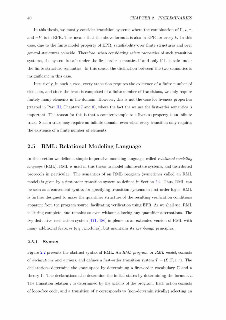
40 CHAPTER 2. PRELIMINARIES
In this thesis, we mostly consider transition systems where the combination of Γ, ι, τ ,
and ¬P , is in EPR. This means that the above formula is also in EPR for every k. In this
case, due to the finite model property of EPR, satisfiability over finite structures and over
general structures coincide. Therefore, when considering safety properties of such transition
systems, the system is safe under the first-order semantics if and only if it is safe under
the finite structure semantics. In this sense, the distinction between the two semantics is
insignificant in this case.
Intuitively, in such a case, every transition requires the existence of a finite number of
elements, and since the trace is comprised of a finite number of transitions, we only require
finitely many elements in the domain. However, this is not the case for liveness properties
(treated in Part III, Chapters 7 and 8), where the fact the we use the first-order semantics is
important. The reason for this is that a counterexample to a liveness property is an infinite
trace. Such a trace may require an infinite domain, even when every transition only requires
the existence of a finite number of elements.
2.5 RML: Relational Modeling Language
In this section we define a simple imperative modeling language, called relational modeling
language (RML). RML is used in this thesis to model infinite-state systems, and distributed
protocols in particular. The semantics of an RML program (sometimes called an RML
model) is given by a first-order transition system as defined in Section 2.4. Thus, RML can
be seen as a convenient syntax for specifying transition systems in first-order logic. RML
is further designed to make the quantifier structure of the resulting verification conditions
apparent from the program source, facilitating verification using EPR. As we shall see, RML
is Turing-complete, and remains so even without allowing any quantifier alternations. The
Ivy deductive verification system [171, 186] implements an extended version of RML with
many additional features (e.g., modules), but maintains its key design principles.
2.5.1 Syntax
Figure 2.2 presents the abstract syntax of RML. An RML program, or RML model, consists
of declarations and actions, and defines a first-order transition system T = (Σ,Γ, ι, τ). The
declarations determine the state space by determining a first-order vocabulary Σ and a
theory Γ. The declarations also determine the initial states by determining the formula ι.
The transition relation τ is determined by the actions of the program. Each action consists
of loop-free code, and a transition of τ corresponds to (non-deterministically) selecting an

2.5. RML: RELATIONAL MODELING LANGUAGE 41
〈rml〉 ::= 〈decls〉 ; 〈actions〉〈decls〉 ::= ε | 〈decls〉; 〈decls〉
| sort s
| relation r : s
| function f : s→ s
| individual v : s
| axiom ϕ
| init ϕ
〈actions〉 ::= ε | 〈actions〉 ; 〈actions〉| action a { 〈cmd〉 }
〈cmd〉 ::= skip do nothing
| abort terminate abnormally
| r (x) := ϕ (x) first-order update of relation r to formula ϕ(x)
| f (x) := t (x) first-order update of function f to term t (x)
| v := ∗ havoc of individual v
| assume ϕ assume formula ϕ holds
| 〈cmd〉 ; 〈cmd〉 sequential composition
| 〈cmd〉 | 〈cmd〉 non-deterministic choice
Figure 2.2: Core syntax of RML. s denotes a sort identifier and s denotes a tuple of sortidentifiers separated by commas. r denotes a relation identifier. f denotes a functionidentifier. v denotes an individual identifier. ϕ denotes a closed first-order formula. adenotes an action identifier. x denotes a tuple of logical variables. t (x) denotes a term withfree logical variables x and ϕ (x) denotes a first-order formula with free logical variables x.

42 CHAPTER 2. PRELIMINARIES
action and executing its code atomically. Thus, an RML program can be understood as a
single loop, where the loop body is a non-deterministic choice between all the actions. The
restriction of each action to loop-free code simplifies the presentation, and it does not reduce
RML’s expressive power, as nested loops can always be converted to a flat loop.
Declarations The declarations of an RML program define:
(i) a set of sorts given by sort declarations;
(ii) a set of sorted relations given by relation declarations;
(iii) a set of sorted functions given by function declarations, and by individual declarations
that define nullary functions;
(iv) a set of first-order axioms given by axiom declarations; and
(v) a set of first-order initial-state formulas that specify the initial states, given by init
declarations.
An RML program defines a first-order transition system specification (Σ,Γ, ι, τ). The
many-sorted first-order vocabulary Σ consists of the declared sorts, relations, and function
symbols. The theory Γ consists of the formulas declared as axioms. The initial states formula
ι is the conjunction of all initial-state formulas.
Actions The transition relation formula τ is determined by the actions of the RML
program. Each action consists of a name and a loop-free body, given by an RML command.
The transition relation formula τ of the whole program is given by the disjunction of the
transition relation formulas associated with each action of the program. Effectively, this
means that each τ -transition is a non-deterministic choice between all the actions of the
program, and that each action is executed atomically. Below we given an intuitive description
of RML commands, and Section 2.5.2 presents their axiomatic semantics and explains how
to translate a command C to its associated transition relation formula τ [C]. Formally, if
the bodies of actions are C1, , . . . , , Ck then the transition relation of the whole program τ is
given by:
τ =∨i
τ [Ci]

2.5. RML: RELATIONAL MODELING LANGUAGE 43
Commands Each command investigates and potentially updates the state, i.e., the value of
the relation and function symbols. The semantics of skip is standard. The semantics of abort
is also standard, and it can be used to define a safety property as part of the RML program,
i.e., the safety property says that the program does not execute an abort command. The
command r(x1, . . . , xn) := ϕ(x1, . . . , xn) is used to update the n-ary relation r to the set of all
n-tuples of elements that satisfy the first-order formula ϕ. For example, r(x1, x2) := (x1 = x2)
updates the binary relation r to the identity relation; r(x1, x2) := r(x2, x1) updates r to its
inverse relation (or transpose); r1(x) := r2(x, v) updates r1 to the set of all elements that
are related by r2 to the current value (interpretation) of the individual v .
The command f (x1, . . . , xn) := t(x1, . . . , xn) is used to update the n-ary function f to
map every n-tuple of elements to the element given by the term t. Note that while relations
are updated to first-order formulas, functions are updated to first-order terms. For example,
f (x) := x updates the function f to the identity function; f (x1, x2) := f (x2, x1) updates f to
its transpose; f (x) := ite(r(x), x, f (x)) updates f to be the identity function for all elements
in r , and leaves it unchanged for all elements not in r .
The havoc command v := ∗ performs a non-deterministic assignment to v , where it can
be assigned to any value (element) of the appropriate sort. The assume command is used
to restrict the executions of the program to those that satisfy the given (closed) first-order
formula. Sequential composition and non-deterministic choice are defined in the usual way.
Syntactic sugars The commands given in Figure 2.2 are the core of RML. Figure 2.3 pro-
vides several useful syntactic sugars for RML, including an assert command, an if-then-else
command, and convenient update commands for relations and functions. Syntactic sugar
also allows to declare individuals inside actions, either as action parameters or via a local
declaration. In both cases, individuals are added to Σ, and use of these individuals is
restricted to the scope of a specific action.
In addition to the syntactic sugars of Figure 2.3, when presenting RML code (e.g.,
Figure 3.1) we allow ourselves to use some shorthands that improve clarity, and are straight-
forward to translate to the official syntax. (In fact, most of these shorthands are supported
by Ivy.) Examples include omission of semicolons, use of infix notation (e.g., u ≤ v rather
than ≤ (u, v)), and using u < v as a shorthand for u ≤ v ∧ u 6= v. We also allow ourselves to
omit sorts if they can be easily inferred (e.g., declare v : s and later use v).
When presenting RML code, we use capital letters for logical variables that are
used in assignment statements. We also allow ourselves to mix variables and ground
terms in assignments, by a natural extension of the assignment syntactic sugar pro-

44 CHAPTER 2. PRELIMINARIES
Syntactic Sugar Desugared RML
action a (v1 : s1, . . . , vn : sn) {C} action a {v1 := ∗; . . . ; vn := ∗;C}Also add declarations for new individuals
v1 : s1, . . . , vn : sn that are local to the scope of a
local v : s := e v := e
Also add a declaration for a new individual v : s
that is local to the action scope
assert ϕ {assume ¬ϕ ; abort} | skip
if ϕ C1 {assume ϕ ; C1} | {assume ¬ϕ}if ϕ C1 else C2 {assume ϕ ; C1} | {assume ¬ϕ ;C2}r (g) := ϕ r (x) := (x = g ∧ ϕ) ∨ (x 6= g ∧ r (x))
f (g) := g f (x) := ite (x = g, g, f (x))
Figure 2.3: Syntactic sugars for RML. In addition to using the notations of Figure 2.2, gdenotes a ground term, g denotes a tuple of ground terms, and equality and between tuplesdenotes the conjunction of the component-wise equalities.
vided by Figure 2.3. For example, we write r(V, c) := p(V) as syntactic sugar for
r(x, y) := (y = c ∧ p(x)) ∨ (y 6= c ∧ r(x, y)). This convenience is also supported by Ivy.
2.5.2 Axiomatic Semantics
We now provide a formal semantics for RML commands by defining a weakest precondition
operator, which also allows us to define the transition relation formula of an RML command.
Weakest precondition of RML commands We define the weakest precondition opera-
tor for RML commands with respect to assertions expressed as closed first-order formulas
over Σ. In this section, we use assertions and formulas interchangeably, and they are always
assumed to be closed. A state satisfies an assertion if it satisfies it in the usual semantics of
many-sorted first-order logic.
Figure 2.4 presents the definition of the weakest precondition operator for RML commands.
The weakest precondition [66] of a command C with respect to an assertion Q, denoted
wp(C,Q), is an assertion Q′ such that every execution of C starting from a state that
satisfies Q′ leads to a state that satisfies Q. Further, wp(C,Q) is the weakest such assertion.
Namely, Q′ |= wp(C,Q) for every Q′ as above. (Note that RML commands are loop-free, so
termination of an RML command is trivial.)

2.5. RML: RELATIONAL MODELING LANGUAGE 45
wp (skip, Q) = Q
wp (abort, Q) = false
wp (r (x) := ϕ (x) , Q) = (∧
Γ→ Q) [ϕ (s) / r (s)]
wp (f (x) := t (x) , Q) = (∧
Γ→ Q) [t (s) / f (s)]
wp (v := ∗, Q) = ∀x. (∧Γ→ Q) [x / v ]
wp (assume ϕ,Q) = ϕ→ Q
wp (C1 ; C2, Q) = wp (C1,wp (C2, Q))
wp (C1 | C2, Q) = wp (C1, Q) ∧ wp (C2, Q)
Figure 2.4: Rules for weakest precondition of RML commands. ϕ [β / α] denotes ϕ withoccurrences of α substituted by β. s denotes a tuple of terms.
∧Γ denotes the conjunction
of all formulas in the theory Γ.
The rules for wp of skip and abort are standard, as are the rules for assume, sequential
composition and non-deterministic choice. The rules for updates of relations and functions
and for havoc are instances of Hoare’s assignment rule [105], applied to the setting of RML
and adjusted for the fact that state mutations are restricted by the axioms in Γ.
Transition relation formulas of RML commands The weakest precondition operator
is closely related to transition relation formulas. Recall that a transition relation formula
has vocabulary Σ ] Σ′, where the primed symbols represent the state after executing the
command. For further details on efficient ways to encode verification conditions (using
weakest precondition operators and transition formulas), see [79, 147]. Here, we use the
following connection to define the transition relation of a command C, denoted by τ [C],
using the weakest precondition operator (as defined in Figure 2.4):
τ [C] = ¬wp (C,¬ψΣ=Σ′)
where:
ψΣ=Σ′ =∧r∈Σ
∀x. r(x)↔ r′(x) ∧∧f∈Σ
∀x. f(x) = f ′(x)
This makes a slight abuse of the definition of wp, since it applies wp to a formula over Σ]Σ′.
However, in this context, the symbols in Σ′ can be treated as additional auxiliary symbols,
without special meaning.
Intuitively, there is a transition from s to s′ if and only if s does not satisfy the weakest
precondition of “not being s′”. This is captured by the above connection, and “not being s′”
is captured by ¬ψΣ=Σ′ . Note further that non-deterministic choice between commands results

46 CHAPTER 2. PRELIMINARIES
in a conjunction in the weakest precondition, and a disjunction in the transition relation.
Similarly, a havoc command results in a universal quantifier in the weakest precondition,
and an existential quantifier in the transition relation.
Recall that an RML program defines a first-order transition system specification:
(Σ,Γ, ι, τ). The transition relation τ given by the disjunction of the transition relations of
each action in the RML program, where the transition relation of each action is computed
from its body via the above definition. Note that when using the syntactic sugar of Figure 2.3
to define an actions with parameters, these parameters are existentially quantified in the
transition relation.
Safety properties The abort commands in the RML program also define a safety property
P . Intuitively, the safety property is that the program does not execute an abort command.
Formally, if the bodies of actions are C1, , . . . , , Ck then the safety property P is given by:
P =∧i
wp (Ci, true)
2.5.3 Quantifier Alternation Structure
One of the design goals of RML is to facilitate verification using EPR. For this, the user must
have visibility and control over the quantifier alternation graph of verification conditions that
result from RML programs and inductive invariants. In the VCs (defined in Section 2.4.2),
the formulas from Γ, ι, and τ appear positively. In RML, the user has direct control over
Γ and ι via declarations. In contrast, τ is computed from the program source. Thus, it is
important that the quantifier structure of τ is clearly apparent from the program source.
In RML, the only quantifiers in τ that are not explicit in the program source are those
that arise from havoc commands (action parameters included), which lead to existential
quantifiers in τ . The close connection between the program source and the quantifier
alternation structure of VCs can be observed in Figure 2.4, and is also manifested by the
following lemma, showing that under certain conditions ∀∗ ∃∗-formulas are closed under wp.
(Recall that τ is given by a negation of wp, so ∀∗ ∃∗ in wp corresponds to ∃∗ ∀∗ in τ .)
Lemma 2.5. Let C be an RML command, and suppose that all assignments to relations
use quantifier-free formulas, and all assume commands, as well as the theory Γ, contain
formulas with ∃∗ ∀∗ prenex normal form. Under these conditions, if Q is a ∀∗ ∃∗-formula,
then so is the prenex normal form of wp(C,Q).
Proof. Straightforward from the rules of Figure 2.4.

2.5. RML: RELATIONAL MODELING LANGUAGE 47
2.5.4 Turing-Completeness
To see that RML is Turing-complete, we can encode a (Minsky) counter machine in RML.
The finite state (program counter) can be encoded using nullary relations. Each counter ci
can be encoded with a unary relation ri. The value of counter ci is the number of elements
in ri. Testing for zero, incrementing, and decrementing counters can all be easily expressed
by RML commands that only use alternation-free formulas in assume statements (see
below). Therefore, RML, as well as the formalism of first-order transition systems, are
Turing-complete, even when restricted not to use any quantifier alternations.
Testing for zero can be done by checking ∀x. ¬ri(x). Incrementing can be done by
local v := ∗ ; assume ¬ri(v) ; ri(v) := true. Decrementing can be done by
local v := ∗ ; assume ri(v) ; ri(v) := false.

Chapter 3
Modeling in First-Order Logic
This chapter is partially based on work published in [186, 187].
This chapter is concerned with the following question: how can we model distributed
algorithms as first-order transition systems? Moreover, we seek to do this in a way that
facilitates verification using the EPR decidable fragment. Recall that we use uninterpreted,
many-sorted, first-order logic. Therefore, modeling a distributed protocol as a first-order
transition system involves some abstraction, since protocols usually employ concepts that
are not definable in uninterpreted first-order logic. We thus aim for a sound abstraction that
is precise enough to allow verification. (As we shall see, in some cases we can exploit the
finite model property of EPR to obtain a form of completeness.)
In order to express concepts in first-order logic, we use suitable sorts, relation symbols,
and function symbols. The sorts and symbols have an intended meaning, but we use them
in uninterpreted first-order logic. To capture part of the intended interpretation, we add a
finite set of first-order axioms. These are first-order formulas that are valid in the intended
interpretation. By adding them to the first-order transition system, we allow the proof
of verification conditions to rely on these axioms. By using only axioms that are valid in
the intended interpretation, we guarantee that the first-order transition system is a sound
abstraction of the actual system or protocol, so any invariant proved for the first-order
transition system is also an invariant of the protocol.
In this chapter, we present encodings for transitive closure of deterministic paths (Sec-
tion 3.3), quorums and cardinality constraints (Section 3.4), and network semantics (Sec-
tion 3.5). Similar encodings for deterministic paths have been used in the past in the context
of heap verification, and we present them in detail for uniformity and to make this thesis self
contained. The encodings for cardinalities and network semantics are more straightforward,
48

3.1. MOTIVATING EXAMPLES 49
and the key novelty is not the encodings themselves, but rather their use as part of an
overall scheme for verification of distributed algorithms in decidable logic, as presented in
the following chapters of this thesis.
3.1 Motivating Examples
To illustrate both the challenges and our solutions, we present two simple examples of
distributed protocols, and their modeling and verification in first-order logic and EPR.
3.1.1 Leader Election in a Ring Protocol
Consider a simple protocol for leader election in a ring [43]. The protocol assumes a
unidirectional ring of unbounded size. That is, nodes are organized in a ring, and messages
can only be sent from each node to its immediate successor in the ring. The protocol also
assumes every node has a unique ID — a natural number known to the node (but initially
not to other nodes), such that no two nodes have the same ID. The protocol performs leader
election by decentralized extrema-finding. Every node starts by sending its own ID to its
successor in the ring. A node forwards messages that contain an ID higher than its own ID.
When a node receives a message with its own ID, it concludes that it has the maximal ID,
and declares itself as a leader. The key safety property of this protocol is that it elects at
most one leader.
This example poses several challenges to modeling in first-order logic. First, note that
the IDs are natural numbers. It is well-known that no finite (or even recursively enumerable)
axiomatization of the natural numbers (including arithmetic and/or uninterpreted relations)
in first-order logic can be complete. Second, the protocol assumes a finite ring topology.
This notion is also not first-order definable. Also, as we shall see, the inductive invariant of
the protocol requires concepts such as paths in the ring — transitive closure of ring edges
— and transitive closure is also not first-order definable. However, using the techniques we
develop in this chapter, we can express this protocol, and its safety proof, in first-order logic.
Figure 3.1 presents an RML model of the leader election protocol. We use a sort node to
represent nodes in the ring network, and a sort id to represent node IDs. The function id
maps every node to its ID. We define a binary relation ≤ on IDs, with axioms for ≤ being
a total order, as explained in Section 3.2. That is, we abstract the real protocol, which
uses natural numbers, to a protocol that uses an arbitrary totally ordered set. The ring
topology is represented by a ternary btw relation, as explained in Section 3.3.3. The idea is
that btw(x, y, z) holds if y is between x and z in the ring, that is, if y is part of the shortest
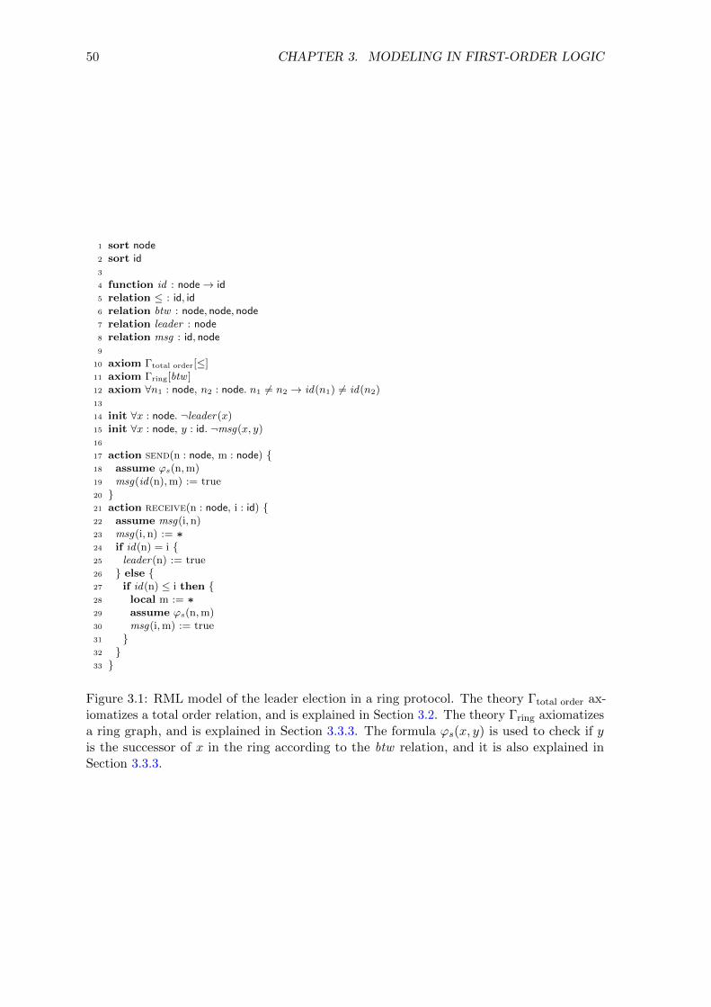
50 CHAPTER 3. MODELING IN FIRST-ORDER LOGIC
1 sort node2 sort id3
4 function id : node→ id5 relation ≤ : id, id6 relation btw : node, node, node7 relation leader : node8 relation msg : id, node9
10 axiom Γtotal order[≤]11 axiom Γring[btw ]12 axiom ∀n1 : node, n2 : node. n1 6= n2 → id(n1) 6= id(n2)13
14 init ∀x : node. ¬leader(x)15 init ∀x : node, y : id. ¬msg(x, y)16
17 action send(n : node, m : node) {18 assume ϕs(n,m)19 msg(id(n),m) := true20 }21 action receive(n : node, i : id) {22 assume msg(i, n)23 msg(i,n) := ∗24 if id(n) = i {25 leader(n) := true26 } else {27 if id(n) ≤ i then {28 local m := ∗29 assume ϕs(n,m)30 msg(i,m) := true31 }32 }33 }
Figure 3.1: RML model of the leader election in a ring protocol. The theory Γtotal order ax-iomatizes a total order relation, and is explained in Section 3.2. The theory Γring axiomatizesa ring graph, and is explained in Section 3.3.3. The formula ϕs(x, y) is used to check if yis the successor of x in the ring according to the btw relation, and it is also explained inSection 3.3.3.

3.1. MOTIVATING EXAMPLES 51
(i.e., acyclic) path from x to z.
The state of the protocol is represented by the leader relation, indicating which nodes
consider themselves leaders; and the msg relation, modeling the network by storing which
messages are in transit. As explained in Section 3.5, this actually models a network with
message dropping, reordering, and duplication; and this protocol is indeed correct under
such network semantics. The model contains two actions: send that models a node sending
its ID to its successor in the ring, and receive that models a node receiving a message.
The safety property of the protocol is expressed by the following first-order formula:
∀x : node, y : node. leader(x) ∧ leader(y)→ x = y (3.2)
Most importantly, the safety of the protocol can be proven with the following inductive
invariant expressed in first-order logic:
∀x : node, y : node. leader(x)→ id(y) ≤ id(x) (3.3)
∀x : node, y : node. msg(id(x), x)→ id(y) ≤ id(x) (3.4)
∀x : node, y : node, z : node. btw(x, y, z) ∧msg(id(x), z)→ id(y) ≤ id(x) (3.5)
Equation (3.3) states that a leader has a maximal ID, and Equation (3.4) similarly states
that a node whose ID is self-pending has a maximal ID. Equation (3.5) involves three nodes,
and it states that a message cannot bypass a node with a higher ID. Note that the invariant is
universally quantified, and the VCs for checking it are in EPR (the only quantifier alternation
edge results from the id function, from node to id). Indeed, this example takes under two
seconds to verify with Ivy and Z3 (on a standard laptop).
The fact that the protocol’s inductive invariant is expressible in first-order logic depends
on the fact that we use btw to represent the ring topology. Note that Equation (3.5) states
that if the ID of node x is pending at node z, then the ID of x is greater than that of every
node between x and z. It is crucial to express this fact, regardless of the length of the path
between x and z. Using an alternative representation of the ring by a binary relation that
represents graph edges, this fact is not first-order expressible. It can be expressed, e.g., using
transitive closure. Thus, the use of the btw relation, with its definitions axioms Γring, is key
to verifying this protocol in first-order logic.
The details of Γring and the btw relation, as well as similar representations for other
classes of graphs, appear in Section 3.3.

52 CHAPTER 3. MODELING IN FIRST-ORDER LOGIC
1 sort node2 sort value3 sort quorum4
5 relation member : node, quorum6 relation vote msg : node, value7 relation decision : value8
9 axiom ∀q1, q2 : quorum. ∃n : node.member(n, q1) ∧member(n, q2)10
11 init ∀x : node, y : value. ¬vote msg(x, y)12 init ∀x : value. ¬decision(x)13
14 action vote(n : node, v : value) {15 assume ∀x : value. ¬vote msg(n, x)16 vote msg(n, v) := true17 }18
19 action decide(v : value) {20 assume ∃q : quorum. ∀n : node. member(n, q)→ vote msg(n, v)21 decision(v) := true22 }
Figure 3.6: RML model of the majority vote toy protocol. For this protocol, we wish toprove decision never contains two different values. We use a sort for quorums with a suitableaxiom stating that any two quorums intersect, as explained in Section 3.4.
3.1.2 Majority Vote Protocol
Consider a set of N nodes that can send messages to each other (all to all communication).
They can decide on a unique value, by having each node vote for a single value, and requiring
a majority for a decision. That is, a value is considered decided if more than N/2 nodes
voted for it. This protocol does not guarantee that some value will be decided (the votes
may split in such a way that no value obtains a majority), but it is safe, in the sense that at
most one value is decided.
This toy protocol illustrates an essential part of the safety argument of many consensus
protocols, such as Paxos [135, 136]. The argument is that since each node only votes for
a single value, and since any two sets of more than N/2 nodes intersect, then at most one
value can obtain a majority of the votes. While straightforward, this argument uses concepts
that are not directly expressible in first-order logic. It uses sets defined by predicates (the
nodes that voted for a value), and relies on the cardinalities of these sets. However, using the
techniques we develop in this chapter, this protocol, and other protocol relying on similar
arguments (including Paxos), can be modeled and verified in first-order logic.
Figure 3.6 presents an RML model of the majority vote protocol. It uses sorts for
nodes and values (node and value), and also a sort quorum for quorums, i.e., majority
sets. This technique is explained in detail in Section 3.4. In a nutshell, we use a relation

3.1. MOTIVATING EXAMPLES 53
member : node, quorum to represent set membership, and to use an axiom to state that any
two quorums intersect (line 9). Then, the condition of having at least N/2 votes for a single
value can be expressed in first-order logic (line 20). This involves an abstraction, since other
than the axiom of line 9, the quorum sort and the member relation are uninterpreted. This is
nevertheless sound, and also precise enough to prove the safety of the majority vote protocol.
The safety property of the protocol, i.e., that at most one value is decided, can be expressed
by the following first-order formula:
∀v1 : value, v2 : value. decision(v1) ∧ decision(v2)→ v1 = v2 (3.7)
The safety of the majority vote protocol can be proven by the following inductive invariant
expressed in first-order logic:
∀n : node, v1 : value, v2 : value. vote msg(n, v1) ∧ vote msg(n, v2)→ v1 = v2 (3.8)
∀v : value. decision(v)→ ∃q : quorum. ∀n : node. member(n, q)→ vote msg(n, v) (3.9)
Equation (3.8) states that every node votes for at most one value, and Equation (3.9) states
that every decided value must be due to a majority vote, i.e., there is a quorum such that all
member of the quorum voted for the decided value. This invariant contains some quantifier
alternations, but the resulting VCs are in EPR. The axiom of line 9 introduces a quantifier
alternation edge from quorum to node, and Equation (3.9) introduces an edge from value to
quorum, and another edge from quorum to node, arising from the negation of the invariant
in the VCs (see Section 2.4). When combined, these edges do not create a cycle, so the VCs
are in EPR. Indeed, this example also takes under two seconds to verify with Ivy and Z3 (on
a standard laptop).
The rest of this chapter explores the issues illustrated by these two toy protocol examples
in more detail, and provides techniques for modeling systems and protocols in first-order
logic. Section 3.2 begins with a short discussion of expressing total orders in first-order logic,
which provides a basis for the technique presented in Section 3.3 for representing paths in
several classes of graphs with outdegree one, in a way that is both sound and complete for
finite models. Section 3.4 discussed the issue of expressing higher-order quantification and
cardinality thresholds, and Section 3.5 discusses the modeling of various network semantics
in first-order logic. We note that while this chapter illustrates the issues using toy examples,
the techniques we present also apply to complex protocol such as Paxos and its variant, and
have led to the first mechanized verification of several protocols, as we shall see in Chapter 4

54 CHAPTER 3. MODELING IN FIRST-ORDER LOGIC
Transitivity ∀x, y, z. x ≤ y ∧ y ≤ z → x ≤ zAntisymmetry ∀x, y. x ≤ y ∧ y ≤ x→ x = y
Totality ∀x, y. x ≤ y ∨ y ≤ x
Successor ϕs(x, y) ≡ x ≤ y ∧ x 6= y ∧ ∀z. x ≤ z ∧ x 6= z → y ≤ z
Figure 3.10: Encoding of a total order in first-order logic. Axioms stating the relation ≤ is atotal order; and a formula for defining the successor relation from ≤.
(for safety proofs), and later in Chapter 7 (for liveness proofs).
3.2 Total Orders
One important example of axioms expressible in first-order logic is the axiomatization of
total orders. In many cases, protocols use natural numbers or integers. A common use is to
enforce a total order on a set of elements. The leader election protocol of Section 3.1.1, which
uses IDs that are natural numbers, is an example of this. Such use of integers or natural
numbers can be captured in first-order logic by adding a binary relation ≤, along with the
axioms listed in Figure 3.10, which precisely capture the properties of a total (linear) order.
These axioms are sound for a finite totally ordered set (e.g., the set of node IDs in the
leader election in a ring protocol of Figure 3.1), and also for infinite totally ordered sets,
such as the natural numbers or the integers. Moreover, the successor relation is expressible
as a first-order formula ϕs over the order relation ≤. This formula, also listed in Figure 3.10,
contains one universal quantifier.
The axioms of Figure 3.10 are universally quantified and do not contain any quantifier
alternations. However, the fact that the successor formula contains a universal quantifier
may lead to quantifier alternations that create a cycle in the quantifier alternation graph.
For example, one may wish to state the following property in an inductive invariant:
∀x, y. ϕs(x, y)→ p(x, y). However, this formula’s prenex normal form has quantifier prefix
∀∗ ∃∗, and it is outside of the EPR fragment. In contrast, the formula ∀x, y. p(x, y)→ ϕs(x, y),
or the formula ϕs(a, b) → p(a, b) where a and b are constant symbols, do not create any
quantifier alternations. Thus, the restrictions of EPR allow some use of the successor formula,
but not general use.
When the total order axioms and successor formula are used for verification such that the
resulting VCs are in EPR, the obtained counterexamples will always be finite (due to EPR’s
finite model property). This means that even if the total order is used as an abstraction

3.3. DETERMINISTIC PATHS 55
Line (total order) RingForest (acyclic
partial function)
Graph withoutdegree one
(partial function)
Figure 3.11: Illustration of classes of graphs with outdegree one. Paths in these graphs canbe captured in the EPR decidable fragment of first-order logic.
for the integers or natural numbers, in the obtained counterexamples its domain will be a
finite totally ordered set. Note that for such models, the ≤ relation is always precisely the
transitive closure of the successor relation defined by the ϕs formula. However, this is not the
case for infinite models. For example, consider the set {0, 1} × N ordered lexicographically.
It satisfies the total order axioms, but ≤ is not equivalent to the transitive closure of the
successor relation. This observation inspires the next section, where we present several
adaptations of the total order axioms and successor formula to represent paths in graphs
with outdegree one.
Another observation worth noting is that it is not possible to keep both the successor
relation and the order relation in the vocabulary and have a complete axiomatization of
the connection between them. That is, if one takes the vocabulary Σ = {s2,≤2}, then
there is no first-order theory Γ that is satisfied by a structure (D, I) if and only if I(≤)
is a total order and is also the reflexive transitive closure of I(s). This can easily be
shown by compactness of first-order logic (e.g., [203]). Interestingly, the following formula
(when taken together with the total order axioms of Figure 3.10) does provide a complete
characterization of transitive closure for finite structures (i.e., as above but restrict D to
be finite) [152]: ∀x, y. x ≤ y ↔ (x = y ∨ ∃z. s(x, z) ∧ z ≤ y). However, since this formula
contains ∀ ∃ quantifier alternation, it is outside of EPR, and does not have a finite model
property. In the next section, we will maintain both completeness for finite structures and
remain in EPR, by using a vocabulary that does not contain the successor (or edge) relation
s, and using ϕs in lieu of it as needed and under the restrictions of EPR.
3.3 Deterministic Paths
One of the main hurdles to using first-order logic in verification is the fact that it cannot
express transitive closure, which is required to express properties and invariant that involve

56 CHAPTER 3. MODELING IN FIRST-ORDER LOGIC
paths in graphs. In this section we present encodings for four classes of graphs, all with
outdegree one, that allow to express graph paths in first-order logic. We say that a graph
has outdegree one if the outdegree of every vertex is at most one (i.e., each vertex has at
most one outgoing edge). The classes we consider are depicted in Figure 3.11. The encodings
in first-order logic are inspired by the total order axioms and the successor formula discussed
in the previous section. These encodings exploit ideas that have been used in the past in
the context of verification of heap manipulating programs [111–113, 133, 194, 195, 223, 224].
However, for the purpose of uniformity, and to make this thesis self contained, we present
the encodings in detail.
For each class of graphs, we present axioms of a path relation, a successor formula that
allows to express graph edges from the path relation, update formulas for manipulating the
graph, and soundness and completeness theorems. The completeness theorems state that any
finite model of the axioms is isomorphic to a graph of the corresponding class. Together with
the finite model property of EPR, this leads to a complete reasoning procedure for deductive
verification of programs manipulating such graphs. That is, every obtained counterexample
corresponds to an actual graph, and the encoding of paths in first-order logic does not lead
to spurious counterexamples.
3.3.1 Line
The first class of graphs we consider is line graphs. That is, a directed graph where every
node has both indegree one and outdegree one, except for two extreme nodes: the minimal
node has indegree zero, and the maximal node has outdegree zero. Since we are interested
in transition systems manipulating this graph, we do not assume that all elements of the
domain are part of the graph structure. This allows us to also express addition and removal
of nodes from the graph. Example uses of this encoding are to represent a queue or a stack
data-structure, in first-order logic. Thus, pushing and popping elements corresponds to
adding and removing elements from the line graph.
The idea for the encoding is to represent the line graph with a transitive relation ≤ that
is total and reflexive only on the elements that are part of the line. For elements that are
part of the line, ≤ represents the reflexive transitive closure of graph edges. Other elements
in the domain that are not part of the line are left outside the ≤ relation. To add or remove
elements from the line, the ≤ relation is updated. Figure 3.12 lists the axioms for the ≤relation (which is the path relation in this case), a successor formula ϕs that derives graph
edges from the ≤ relation, several useful first-order queries, and update code for adding and
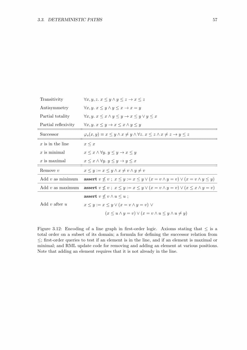
3.3. DETERMINISTIC PATHS 57
Transitivity ∀x, y, z. x ≤ y ∧ y ≤ z → x ≤ zAntisymmetry ∀x, y. x ≤ y ∧ y ≤ x→ x = y
Partial totality ∀x, y. x ≤ x ∧ y ≤ y → x ≤ y ∨ y ≤ xPartial reflexivity ∀x, y. x ≤ y → x ≤ x ∧ y ≤ y
Successor ϕs(x, y) ≡ x ≤ y ∧ x 6= y ∧ ∀z. x ≤ z ∧ x 6= z → y ≤ z
x is in the line x ≤ xx is minimal x ≤ x ∧ ∀y. y ≤ y → x ≤ yx is maximal x ≤ x ∧ ∀y. y ≤ y → y ≤ x
Remove v x ≤ y := x ≤ y ∧ x 6= v ∧ y 6= v
Add v as minimum assert v 6≤ v ; x ≤ y := x ≤ y ∨ (x = v ∧ y = v) ∨ (x = v ∧ y ≤ y)
Add v as maximum assert v 6≤ v ; x ≤ y := x ≤ y ∨ (x = v ∧ y = v) ∨ (x ≤ x ∧ y = v)
Add v after u
assert v 6≤ v ∧ u ≤ u ;
x ≤ y := x ≤ y ∨ (x = v ∧ y = v) ∨(x ≤ u ∧ y = v) ∨ (x = v ∧ u ≤ y ∧ u 6= y)
Figure 3.12: Encoding of a line graph in first-order logic. Axioms stating that ≤ is atotal order on a subset of its domain; a formula for defining the successor relation from≤; first-order queries to test if an element is in the line, and if an element is maximal orminimal; and RML update code for removing and adding an element at various positions.Note that adding an element requires that it is not already in the line.

58 CHAPTER 3. MODELING IN FIRST-ORDER LOGIC
removing nodes from the line.
The soundness and completeness of this encoding are given by the following theorems.
Theorem 3.13 (Line Soundness). For any line graph G = (V,E), and any additional set
of nodes U disjoint from V , let s = (D, I) be the first-order structure given by D = V ] U ,
I(≤) = E∗ ⊆ V × V , where E∗ is the reflexive transitive closure of E (when considered over
the carrier set V ). Then, s satisfies the axioms of Figure 3.12, and in addition we have the
following (items i and ii are by construction, and stated only for uniformity with the next
theorem):
(i) D = V ] U ;
(ii) for any two elements u, v ∈ D, s |= u ≤ v if and only if (u, v) ∈ E∗;
(iii) for any two elements u, v ∈ D, s |= ϕs(u, v) (where ϕs is taken from Figure 3.12) if
and only if (u, v) ∈ E; and
(iv) for any element v ∈ D, s |= v ≤ v if and only if v ∈ V .
Moreover, let G′ = (V ′, E′) and U ′ be obtained from G,U by one of the updates of Figure 3.12,
and let s′ be the structure defined from G′, U ′ as s is defined from G,U , then s, s′ |= τ , where
τ is the transition relation of the update of Figure 3.12.
Theorem 3.14 (Line Completeness). For any finite structure s = (D, I) that satisfies the
axioms of Figure 3.12, there is a line graph G = (V,E) and additional set of nodes U , such
that the following holds:
(i) D = V ] U ;
(ii) for any two elements u, v ∈ D, s |= u ≤ v if and only if (u, v) ∈ E∗; and
(iii) for any two elements u, v ∈ D, s |= ϕs(u, v) (where ϕs is taken from Figure 3.12) if
and only if (u, v) ∈ E; and
(iv) for any element v ∈ D, s |= v ≤ v if and only if v ∈ V .
Moreover, let s and s′ be two structures with the same domain that satisfy the axioms of
Figure 3.12 such that s, s′ |= τ , where τ is the transition relation of one of the updates
of Figure 3.12. Then, the line graph corresponding to s′ is obtained from the line graph
corresponding to s by the update from Figure 3.12 corresponding to τ .
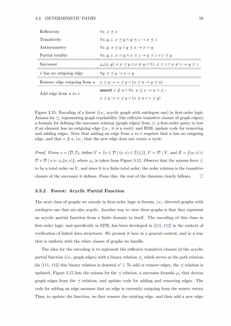
3.3. DETERMINISTIC PATHS 59
Reflexivity ∀x. x � xTransitivity ∀x, y, z. x � y ∧ y � z → x � zAntisymmetry ∀x, y. x � y ∧ y � x→ x = y
Partial totality ∀x, y, z. x � y ∧ x � z → y � z ∨ z � y
Successor ϕs(x, y) ≡ x � y ∧ x 6= y ∧ ∀z. x � z ∧ x 6= z → y � z
x has no outgoing edge ∀y. x � y → x = y
Remove edge outgoing from u x � y := x � y ∧ (x � u→ y � u)
Add edge from u to vassert v 6� u ∧ ∀x. u � x→ u = x ;
x � y := x � y ∨ (x � u ∧ v � y)
Figure 3.15: Encoding of a forest (i.e., acyclic graph with outdegree one) in first-order logic.Axioms for �, representing graph reachability (the reflexive transitive closure of graph edges);a formula for defining the successor relation (graph edges) from �; a first-order query to testif an element has no outgoing edge (i.e., it is a root); and RML update code for removingand adding edges. Note that adding an edge from u to v requires that u has no outgoingedge, and that v 6� u, i.e., that the new edge does not create a cycle.
Proof. Given s = (D, I), define V = {v ∈ D | (v, v) ∈ I(≤)}, U = D \ V , and E = {(u, v) ∈D ×D | s |= ϕs(u, v)}, where ϕs is taken from Figure 3.12. Observe that the axioms force ≤to be a total order on V , and since it is a finite total order, the order relation is the transitive
closure of the successor it defines. From this, the rest of the theorem clearly follows.
3.3.2 Forest: Acyclic Partial Function
The next class of graphs we encode in first-order logic is forests, i.e., directed graphs with
outdegree one that are also acyclic. Another way to view these graphs is that they represent
an acyclic partial function from a finite domain to itself. The encoding of this class in
first-order logic, and specifically in EPR, has been developed in [111, 112] in the context of
verification of linked data structures. We present it here in a general context, and in a way
that is uniform with the other classes of graphs we handle.
The idea for the encoding is to represent the reflexive transitive closure of the acyclic
partial function (i.e., graph edges) with a binary relation �, which serves as the path relation.
(In [111, 112] this binary relation is denoted n∗.) To add or remove edges, the � relation is
updated. Figure 3.15 lists the axioms for the � relation, a successor formula ϕs that derives
graph edges from the � relation, and update code for adding and removing edges. The
code for adding an edge assumes that no edge is currently outgoing from the source vertex.
Thus, to update the function, we first remove the existing edge, and then add a new edge.

60 CHAPTER 3. MODELING IN FIRST-ORDER LOGIC
The code further requires that the new edge does not create a cycle, i.e., that the source of
the new edge is not reachable from its target, and this condition is expressible using the �relation.
The soundness and completeness of this encoding are given by the following theorems.
Theorem 3.16 (Forest Soundness). For any directed forest G = (V,E), i.e., an acyclic
directed graph where the outdegree of any vertex is at most one, let s = (D, I) be the first-order
structure given by D = V , I(�) = {(u, v) ∈ V × V | (u, v) ∈ E∗}, where E∗ is the reflexive
transitive closure of E. Then, s satisfies the axioms of Figure 3.15, and in addition we have
the following:
(i) for any two elements u, v ∈ D, s |= u � v if and only if (u, v) ∈ E∗; and
(ii) for any two elements u, v ∈ D, s |= ϕs(u, v) (where ϕs is taken from Figure 3.15) if
and only if (u, v) ∈ E.
Moreover, let G′ = (V,E′) be a directed forest obtained from G by addition or removal of an
edge, and let s′ be the structure defined from G′ as s is defined from G, then s, s′ |= τ , where
τ is the transition relation of the suitable update code in Figure 3.15.
Theorem 3.17 (Forest Completeness). For any finite structure s = (D, I) that satisfies the
axioms of Figure 3.15, there is a directed forest G = (D, E) such that the following holds:
(i) for any two elements u, v ∈ D, s |= u � v if and only if (u, v) ∈ E∗; and
(ii) for any two elements u, v ∈ D, s |= ϕs(u, v) (where ϕs is taken from Figure 3.15) if
and only if (u, v) ∈ E.
Moreover, let s and s′ be two structures with the same domain that satisfy the axioms of
Figure 3.15 such that s, s′ |= τ , where τ is the transition relation of the edge addition or
removal code listed in Figure 3.15. Then, the graph corresponding to s′ is obtained from the
graph corresponding to s by a suitable edge addition or removal corresponding to τ .
Proof. Given s = (D, I), define E = {(u, v) ∈ D × D | s |= ϕs(u, v)}, where ϕs is taken
from Figure 3.15. With this definition, and since D is finite, the theorem easily follows. For
further details see [111].
3.3.3 Ring
The next class of graphs we consider is rings. That is, a directed connected graph where
every vertex has both indegree and outdegree exactly one. Any such ring is isomorphic to Zn,

3.3. DETERMINISTIC PATHS 61
Cyclicity ∀x, y, z. btw(x, y, z)→ btw(y, z, x)
Transitivity ∀w, x, y, z. btw(w, x, y) ∧ btw(w, y, z)→ btw(w, x, z)
Antisymmetry & Irreflexivity ∀x, y, z. btw(x, y, z)→ ¬btw(x, z, y)
Totality ∀x, y, z. x 6= y ∧ x 6= z ∧ y 6= z → btw(x, y, z) ∨ btw(x, z, y)
Successor ϕs(x, y) = ∀z.z 6= x ∧ z 6= y → btw(x, y, z)
Figure 3.18: Encoding of a ring in first-order logic. Axioms stating that btw represents aring comprising the entire domain; and a formula for defining the successor relation (ringedges) from btw . The query btw(x, y, z) represents the fact that x, y, and z are distinctelements, and that y is between x and z in the ring. That is, y is part of the shortest (i.e.,acyclic) path from x to z.
i.e., {0, . . . , n− 1} with arithmetic modulo n. For Zn, the ring edges (i.e., successor relation)
are defined by E ={
(x, y) ∈ Zn2 | y = x+ 1 mod n}
. In this topology, any element is
reachable from any element via the successor relation. That is, the transitive closure of
the successor relation is trivial (a clique). In this setting, the non-trivial facts about paths
in the ring involve three elements. For distinct elements x, y, z, it may be the case that
y is between x and z in the ring, or that it is not (in which case z is between x and y).
Formally, y is between x and z if y is part of the shortest (i.e., acyclic) path from x to
z. We define the ternary btw relation to capture this fact. For Zn, btw is defined by:
btw(x, y, z) ≡ x < y < z ∨ z < x < y ∨ y < z < x.
We shall now see that a ring can be modeled in way that is similar to the modeling of
a line (Section 3.3.1) and a forest (Section 3.3.2), by using the ternary btw relation as the
path relation. That is, the btw relation admits a first-order axiomatization via universal
formulas, the successor relation is definable from btw using a single universal quantifier, and
the axiomatization is complete for finite structures. Figure 3.18 lists the axiomatization
of btw and the definition of the successor relation (graph edges) from btw . The axioms
comprise Γring used in the leader election protocol of Figure 3.1. Recall that for that example,
this encoding allowed us to verify the protocol using an inductive invariant expressible in
first-order logic, i.e., without using a logic that supports transitive closure.
The soundness and completeness of the encoding are given by the following theorems.
Theorem 3.19 (Ring Soundness). For any n ∈ N, let s = (D, I) be the first-order structure
given by D = Zn and I(btw) = {(x, y, z) ∈ Zn3 | x < y < z ∨ z < x < y ∨ y < z < x}. Then,
s satisfies the axioms of Figure 3.18, and in addition we have the following:
(i) for any three elements u, v, w ∈ D, s |= btw(u, v, w) if and only if

62 CHAPTER 3. MODELING IN FIRST-ORDER LOGIC
u < v < w ∨ w < u < v ∨ v < w < u; and
(ii) for any two elements u, v ∈ D, s |= ϕs(u, v) (where ϕs is taken from Figure 3.18) if
and only if v = u+ 1 mod n.
Theorem 3.20 (Ring Completeness). Any finite structure s = (D, I) that satisfies the
axioms of Figure 3.18 is isomorphic to Z|D|. That is, there exists a bijection f : D → Z|D|such that:
(i) for any three elements u, v, w ∈ D, s |= btw(u, v, w) if and only if
f(u) < f(v) < f(w) ∨ f(w) < f(u) < f(v) ∨ f(v) < f(w) < f(u); and
(ii) for any two elements u, v ∈ D, s |= ϕs(u, v) (where ϕs is taken from Figure 3.18) if
and only if f(v) = f(u) + 1 mod |D|.
Proof. Let a denote an arbitrary element in D. Define an order relation v on D by
v = {(x, y) ∈ D2 | x = y ∨ x = a ∨ btw(a, x, y)}. The axioms of Figure 3.18 imply that
this relation is a total order. Therefore, (D,v) is isomorphic to (Z|D|,≤). Let f be the
isomorphism, then (i) and (ii) hold for this f .
Note that for a ring, we do not present update formulas. In this thesis, we use the ring
encoding to model a static ring network topology. For an evolving ring, it may be the case
that the graph will not always maintain a ring form (e.g., edge removal must break the ring).
In such cases, the general encoding presented in the next section can be used.
3.3.4 General Partial Function
We now generalize the ideas of the previous sections to encode paths of a general graph
where the outdegree of every vertex is at most one (i.e., the graph may contain cycles).
Another way to view such a graph is as a partial function from V to V , which may be cyclic.
As before, the idea is to use a path relation, here a ternary relation p, with universally
quantified axioms, from which the graph edges can be recovered using a first-order query
with a single universal quantifier. Moreover, updates to the graph such as addition and
removal of edges can be expressed as updates to p.
Unlike in the acyclic case of Section 3.3.2, when the graph may be cyclic, reachability
(i.e., transitive closure of edges) is not enough to recover the graph. Instead, we combine the
ideas of Sections 3.3.1 to 3.3.3 and define a ternary relation p, such that for every w, the
binary relation p(w, ·, ·) satisfies the axioms of a line graph from Section 3.3.1. Intuitively,
the elements of the line are the elements reachable from w, and they are ordered by the

3.3. DETERMINISTIC PATHS 63
Transitivity ∀w, x, y, z. p(w, x, y) ∧ p(w, y, z)→ p(w, x, z)
Antisymmetry ∀w, x, y. p(w, x, y) ∧ p(w, y, x)→ x = y
Partial totality ∀w, x, y. p(w, x, x) ∧ p(w, y, y)→ p(w, x, y) ∨ p(w, y, x)
Partial reflexivity ∀w, x, y. p(w, x, y)→ p(w, x, x) ∧ p(w, y, y)
Cycle maximality ∀x, y. p(x, x, y)→ x = y
Transitivity of reachability ∀x, y, z. p(x, y, y) ∧ p(y, z, z)→ p(x, z, z)
Path consistency ∀w, x, y, z. p(x, y, z) ∧ p(x, z, w) ∧ y 6= z → p(y, z, w)
Successor ϕs(x, y) = p(x, y, y) ∧ ∀z. p(x, z, z)→ p(x, y, z)
y reachable from x p(x, y, y)
x is on a cycle p(x, x, x)
y is between x and z x 6= y ∧ x 6= z ∧ y 6= z ∧ p(x, y, z)
x has no outgoing edge ∀y.¬p(x, y, y)
Remove edge outgoing from u p(x, y, z) := p(x, y, z) ∧ x 6= u ∧ (p(x, u, u)→ p(x, z, u))
Add edge from u to v
assert ∀x.¬p(u, x, x) ;
p(x, y, z) := p(x, y, z) ∨ ((p(x, u, u) ∨ x = u) ∧ ¬p(x, z, z) ∧(((p(x, y, u) ∨ y = v) ∧ (p(v, z, z) ∨ z = v)) ∨(p(v, y, z) ∧ z 6= v) ))
Figure 3.21: Encoding of a general (i.e., possibly cyclic) graph with outdegree one in first-order logic. Axioms for a ternary path relation p that captures graph reachability as wellas the structure of cycles; a formula for defining the successor relation (graph edges) fromp; first-order queries to test graph reachability, cycles, order of elements on cycles (i.e.,betweenness), and if an element has no outgoing edge (i.e., it is a root); and RML updatecode for removing and adding edges. Note that adding an edge from u to v requires that uhas no outgoing edge. For every element w, the binary relation p(w, ·, ·) is a reflexive totalorder on the elements reachable from w, ordered by their shortest (i.e., acyclic) distancefrom w. The first (i.e, minimal) element in the line is w’s successor, and if w is on a cycle, witself will be the last (i.e., maximal) element on the line.

64 CHAPTER 3. MODELING IN FIRST-ORDER LOGIC
(shortest) distance from w. The first (i.e, minimal) element in the line is w’s successor. If w
is on a cycle, then w itself will be the maximal element in the line defined by p(w, ·, ·). Note
that it may be the case that p(w, ·, ·) is empty, in which case w has no successor. It may
also be the case that w is both the first and last element (i.e., p(w, ·, ·) = {(w,w)}), which
means w is its own successor (i.e., it has a self edge).
Formally, let (V,E) be a directed graph where the outdegree of each vertex is at most
one. Let us define the following ternary relation over V :
P =
{(x, y, z) ∈ V 3
∣∣∣∣∣ ∃n ∈ N. ∃x1, . . . , xn ∈ V.(n−1∧i=1
(xi, xi+1) ∈ E)∧
∧1≤i<j≤n
xi 6= xj
∧ (x, x1) ∈ E ∧(
n∨i=1
xi = y
)∧ xn = z
}(3.22)
That is, P contains the (x, y, z)’s such that both y and z are reachable from x by one or
more applications of E, and the distance from x to y is less than or equal to the distance
from x to z. In other words, y is on the acyclic path from x to z. This is similar to btw of
Section 3.3.3, but it may also hold when x, y and z are not distinct. Note that (x, y, y) ∈ Piff y is reachable from x, and that (x, x, x) ∈ P iff x is on a cycle. In this case, P will also
contain (x, y, x) for every y reachable from x, and will not contain (x, x, y) for any y 6= x.
A ternary path relation p whose intended interpretation is according to P defined above
can be axiomatized by universally quantified formulas. Figure 3.21 lists the axiomatization for
p, along with a successor formula ϕs that derives graph edges from p with a single universal
quantifier, several useful first-order queries, and update code for adding and removing edges.
The code for adding an edge assumes that no edge is currently outgoing from the source
vertex. Thus, to update the function, we first remove the existing edge, and then add a new
edge. (Unlike Figure 3.15, the code does not require that the new edge does not create a
cycle.)
The soundness and completeness of this encoding are given by the following theorems.
Theorem 3.23 (General Partial Function Soundness). For any directed graph G = (V,E)
where the outdegree of any vertex is at most one, let s = (D, I) be the first-order structure
given by D = V , I(p) = P , where P is given by Equation (3.22). Then, s satisfies the
axioms of Figure 3.21, and in addition we have the following:
(i) for any three elements u, v, w ∈ D, s |= p(u, v, w) if and only if (u, v, w) ∈ P where P
is defined from G by Equation (3.22); and
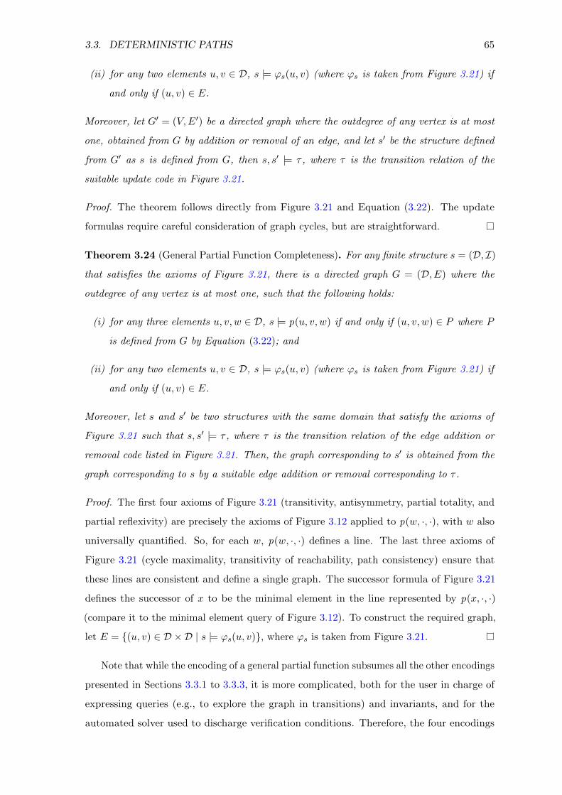
3.3. DETERMINISTIC PATHS 65
(ii) for any two elements u, v ∈ D, s |= ϕs(u, v) (where ϕs is taken from Figure 3.21) if
and only if (u, v) ∈ E.
Moreover, let G′ = (V,E′) be a directed graph where the outdegree of any vertex is at most
one, obtained from G by addition or removal of an edge, and let s′ be the structure defined
from G′ as s is defined from G, then s, s′ |= τ , where τ is the transition relation of the
suitable update code in Figure 3.21.
Proof. The theorem follows directly from Figure 3.21 and Equation (3.22). The update
formulas require careful consideration of graph cycles, but are straightforward.
Theorem 3.24 (General Partial Function Completeness). For any finite structure s = (D, I)
that satisfies the axioms of Figure 3.21, there is a directed graph G = (D, E) where the
outdegree of any vertex is at most one, such that the following holds:
(i) for any three elements u, v, w ∈ D, s |= p(u, v, w) if and only if (u, v, w) ∈ P where P
is defined from G by Equation (3.22); and
(ii) for any two elements u, v ∈ D, s |= ϕs(u, v) (where ϕs is taken from Figure 3.21) if
and only if (u, v) ∈ E.
Moreover, let s and s′ be two structures with the same domain that satisfy the axioms of
Figure 3.21 such that s, s′ |= τ , where τ is the transition relation of the edge addition or
removal code listed in Figure 3.21. Then, the graph corresponding to s′ is obtained from the
graph corresponding to s by a suitable edge addition or removal corresponding to τ .
Proof. The first four axioms of Figure 3.21 (transitivity, antisymmetry, partial totality, and
partial reflexivity) are precisely the axioms of Figure 3.12 applied to p(w, ·, ·), with w also
universally quantified. So, for each w, p(w, ·, ·) defines a line. The last three axioms of
Figure 3.21 (cycle maximality, transitivity of reachability, path consistency) ensure that
these lines are consistent and define a single graph. The successor formula of Figure 3.21
defines the successor of x to be the minimal element in the line represented by p(x, ·, ·)(compare it to the minimal element query of Figure 3.12). To construct the required graph,
let E = {(u, v) ∈ D ×D | s |= ϕs(u, v)}, where ϕs is taken from Figure 3.21.
Note that while the encoding of a general partial function subsumes all the other encodings
presented in Sections 3.3.1 to 3.3.3, it is more complicated, both for the user in charge of
expressing queries (e.g., to explore the graph in transitions) and invariants, and for the
automated solver used to discharge verification conditions. Therefore, the four encodings

66 CHAPTER 3. MODELING IN FIRST-ORDER LOGIC
presented are all useful, and as a rule one should use the simplest encoding possible. For
example, if a routing protocol maintains a forwarding graph that never contains cycles, it is
preferable to use the encoding of Section 3.3.2 (which uses a binary relation), rather than
the encoding presented here (which uses a ternary relation).
3.4 Higher-Order Logic and Cardinality Thresholds
An additional hurdle to using first-order logic in verification is the fact that algorithms and
their invariants often use higher-order quantification, as well as set cardinalities. A common
pattern in distributed algorithms is to use cardinality thresholds. For example, an algorithm
may wait until an operation is acknowledged by at least half of the nodes in the system.
Expressing such an algorithm requires defining sets by predicates (e.g., the set of nodes from
which some message was received), and also expressing constraints over cardinalities of such
sets (e.g., that this set contains at least N2 nodes, where N is the total number of nodes).
Another reason an algorithm may require higher-order quantification is if it uses sets
or functions as values. For example, consider an algorithm in which messages contain a set
of nodes as one of the message fields. Then, the set of messages sent so far (which may be
part of the state of the system) is a set of tuples, where one of the elements in the tuples is
itself a set of nodes. Similarly, messages may contain maps, which are naturally modeled
by functions (e.g., a message may contain a map from nodes to values). In such cases, the
invariants needed to prove the algorithms will usually include higher-order quantification,
i.e., quantification over sets and functions.
3.4.1 Expressing Higher-Order Logic
While higher-order logic cannot be fully reduced to first-order logic, it is well-known [203]
that we can partly express higher-order concepts in first-order logic in the following way.
Sets Suppose we want to express quantification over sets of nodes. We add a new sort
called nodeset, and a binary relation member : node, nodeset. We then use member(n, s)
instead of n ∈ s, and express quantification over sets of nodes as quantification over nodeset.
Typically, we will need to add first-order assumptions or axioms to correctly express the
algorithm and to prove its inductive invariant. For example, the algorithm may set s to
the empty set as part of a transition. We can express this by the following (RML) code:
s := ∗ ; assume ∀x : node.¬member(x, s).
3.4. HIGHER-ORDER LOGIC AND CARDINALITY THRESHOLDS 67
Functions Functions can be encoded as first-order elements in a similar way. Suppose
messages in the algorithm contain a map from nodes to values. In this case, we can add a new
first-order sort called map, and a function symbol apply : map, node→ value. Then, we can
use apply(m,n) instead of m(n), and replace quantification over functions with quantification
of the first-order sort map. As before, we may need to add axioms that capture some of the
intended second-order meaning of the sort map.
Incompleteness While this encoding is sound (as long as we only use axioms that are
valid in the higher-order interpretation), it is not complete. The reason is that the encoding
does not force the interpretation of sorts like nodeset or map to include all the sets or
functions according to the higher-order semantics. In the context of deductive verification,
this means that an inductive invariant that is correct in the higher-order semantics can
actually have a counterexample to induction in the first-order semantics. However, in the
verification projects presented in this thesis, we did not experience this incompleteness to
be a practical obstacle for verification in first-order logic. Namely, we did not encounter a
spurious counterexample arising from the incompleteness of encoding higher-order concepts
(sets, functions) in first-order logic.
3.4.2 Quorums and Cardinality Thresholds
Many distributed protocols use cardinality thresholds to define quorums required for various
operations. This was illustrated in Section 3.1.2 for a toy protocol. Realistic protocols also
use similar principles. For example, a protocol may wait for at least N2 nodes to confirm a
proposal before committing a value, where N is the total number of nodes. This is often
used to ensure consistency in consensus algorithms. In Byzantine failure models, a common
threshold is 2N3 , where at most a third of the nodes may be Byzantine.
First-order logic cannot completely capture set cardinality thresholds. However, this
thesis exploits the fact that protocol correctness commonly relies on rather simple properties
that are implied by the cardinality threshold, and that these properties can be encoded in
first-order logic. The idea is to use a variant of the encoding presented in Section 3.4.1,
and to introduce a sort for quorums defined by a certain threshold, and a membership
relation member between nodes and quorums. Then, properties that are needed for protocol
correctness can be axiomatized in first-order logic. Below we present several examples of
this general principle.
Note that once a sort quorumt has been created for sets of nodes with more than t nodes,
the condition |{n : node | ϕ(n)}| > t, i.e., there are more than t nodes for which ϕ holds,
68 CHAPTER 3. MODELING IN FIRST-ORDER LOGIC
can be expressed in first-order logic as: ∃q : quorumt. ∀n : node. member(n, q)→ ϕ(n). This
technique has been used in the example of Figure 3.6, and is one of the key ingredients to
verification of Paxos protocols presented in Chapter 4 and appendix A.
Below we present several example of first-order properties of quorums that can be
expressed as first-order axioms and used for verifying distributed protocols in first-order
logic. We use N to denote the total number of nodes in the system, and we overload the
relation symbol member as a binary relation between nodes and quorums of various sorts.
Majority sets Many protocols use sets of at least N2 nodes. This threshold ensures that
any two such sets intersect, a property that is crucial for many consensus protocols in order
to maintain consistency. This property can be expressed in first order logic (as was done in
Figure 3.6):
∀q1, q2 : quorum N2. ∃n : node. member(n, q1) ∧member(n, q2)
Byzantine majorities Many Byzantine consensus algorithms use sets of at least 2N3
nodes as quorums, assuming that less than N3 nodes may be Byzantine. The key property of
this threshold is that any two quorums intersect at a non-Byzantine node. This can also
be expressed in first-order logic, using the relation byz : node, which represents Byzantine
nodes:
∀q1, q2 : quorum 2N3. ∃n : node. ¬byz (n) ∧member(n, q1) ∧member(n, q2)
Fast quorums Another interesting example is Fast Paxos [138], a variant of Multi-Paxos
that improves its latency. This protocol uses two kinds of quorums, fast quorums and
classical quorums. These quorums have the property that any two classic quorums intersect,
and any classic quorum and two fast quorums intersect. This can be expressed using two
sorts, quorumf and quorumc, as follows:
∀q1, q2 : quorumc. ∃n : node. member(n, q1) ∧member(n, q2)
∀qc : quorumc, q1, q2 : quorumf . ∃n : node. member(n, qc) ∧member(n, q1) ∧member(n, q2)
Reliable broadcast As a final example, we consider a classical protocol for reliable
broadcast that tolerates up to N3 Byzantine faults (see e.g., [144, Figure 6]). The protocol
uses two types of quorums, with thresholds of N3 and 2N
3 . For our purposes, the important
point is that the correctness of the protocol relies on the following three properties:

3.5. NETWORK SEMANTICS 69
(i) every set of at least N3 nodes contains a non-Byzantine node;
(ii) there is a set of more than 2N3 non-Byzantine nodes; and
(iii) every set of at least 2N3 nodes contains a subset of at least N
3 non-Byzantine nodes.
The correctness of the protocol relies solely on these properties, and fortunately, they can be
expressed in first-order logic as follows:
(i) ∀q : quorum N3. ∃n : node. member(n, q) ∧ ¬byz (n)
(ii) ∃q : quorum 2N3. ∀n : node. member(n, q)→ ¬byz (n)
(iii) ∀q : quorum 2N3. ∃q′ : quorum N
3. ∀n : node. member(n, q′)→ ¬byz (n) ∧member(n, q)
Soundness and trusted base The presented technique abstracts cardinality thresholds
in first-order logic by adding axioms to the first-order transition system (i.e., to Γ). This is
sound, so long as the properties are indeed implied by the cardinality thresholds themselves.
For example, the fact that any two quorums intersect is implied if the quorums are defined
with the threshold N2 , but not if they are defined with N
3 . From the viewpoint of the entire
verification process, adding these properties as axioms creates a new proof obligation, to
show that they follow from the thresholds. In this thesis, we focus on the first-order part
of the verification, and treat the axioms as part of the “trusted base” of the verification
process. We also note that these axioms are reusable across many protocols, and having a
trusted library of axioms is a reasonable approach in this case.
However, it is entirely possible to eliminate the first-order properties from the trusted
base by mechanizing the proof that shows they are implied by the thresholds. This can
be done either by interactive theorem proving, which is already partially supported by Ivy
(and used in [219] to prove that N2 majorities intersect); or by using other decidable logics
that support direct reasoning about set cardinalities, such as BAPA (Boolean Algebra and
Presburger Arithmetic) [131].
3.5 Network Semantics
We now discuss two issues related specifically to modeling of distributed algorithms: modeling
the semantics of the underlying communication network, and modeling concurrency and
asynchrony.
70 CHAPTER 3. MODELING IN FIRST-ORDER LOGIC
3.5.1 Communication Channel Semantics
In distributed computing, any message passing algorithm must assume some semantics for the
communication channels it uses. When verifying the algorithm, it should be verified under
this semantics. For example, one algorithm may only be correct if messages are received in
the same order as they were sent, and another algorithm may be correct even if messages
can be reordered by the network. Another common distinction is whether messages may be
duplicated by the network, i.e., is it possible for a message to be received more times than it
was sent. In this section we show that network models can be easily encoded in first-order
logic, and present the encodings of three common asynchronous communication models:
reordering with duplication, reordering without duplication, and FIFO (first-in-first-out, i.e.,
no reordering and no duplication).
Figure 3.25 presents the encoding of the three network models in first-order logic using
RML syntax. Note that each model may also be modified to allow message dropping, by
adding receive transitions that do nothing with the received message. The encoding presented
here is focused on safety proofs. For liveness, we must also record which messages have been
received, and add suitable fairness assumptions for the network. For example, that every
message sent is eventually received, or that every message that is sent infinitely often is
received infinitely often. These can also naturally be modeled in using a first-order formalism,
as presented in Chapter 7.
Below we provide more details on each of the encodings listed in Figure 3.25.
Reordering with duplication A channel with reordering and duplication is represented
by a relation. Since messages may be duplicated, there is no need to “count” how many
times a message was sent. Accordingly, the receive operation may non-deterministically
remove the received message from the relation, or leave it there.
Reordering without duplication A channel with reordering but no duplication is also
represented by a relation, but here we also use a new sort msg that serves as a unique message
identifier. The send code obtains a fresh identifier and inserts a tuple to the relation, and
the receive code removes a single tuple from the relation. Essentially, we encode a multiset
in a set using unique tags.
FIFO A FIFO (first-in-first-out) channel is one that neither duplicates nor reorders
messages. We represent it using a line graph of messages, exploiting the technique presented
in Section 3.3.1. Messages are represented by a sort msg, with immutable functions field1 :

3.5. NETWORK SEMANTICS 71
Network Model Declarations and Send Code Receive Code
Reordering w/Duplication
relation msg : s1, . . . , skinit ∀x1, . . . , xk. ¬msg(x1, . . . , xk)
msg(f1, . . . , fk) := true
f1, . . . , fk := ∗assume msg(f1, . . . , fk)msg(f1, . . . , fk) := ∗
Reordering w/oDuplication
sort msgrelation msg : msg, s1, . . . , skinit ∀m,x1, . . . , xk. ¬msg(m,x1, . . . , xk)
local m : msg := ∗assume ∀x1, . . . , xk. ¬msg(m,x1, . . . , xk)msg(m, f1, . . . , fk) := true
f1, . . . , fk := ∗local m : msg := ∗assume msg(m, f1, . . . , fk)msg(m,x1, . . . , xk) := false
FIFO
sort msgfunction field1 : msg→ s1, . . . ,fieldk : msg→ skrelation ≤: msg,msgaxiom Γline[≤]init ∀x. x 6≤ x
local m : msg := ∗assume m 6≤ m ∧∧k
i=1 fieldi(m) = fiinsert-as-min[≤](m)
f1, . . . , fk := ∗local m : msg := ∗assume is-max[≤](m)
assume∧k
i=1 fieldi(m) = firemove[≤](m)
Figure 3.25: Encoding of a network models in first-order logic. Declarations, send code,and receive code, are presented for encoding message channels for messages with multiplefields f1 : s1, . . . , fk : sk. The message source and destination can be encoded as fields ifneeded (e.g., in broadcast communication, only the message source is needed). The sendcode assumes the individuals f1, . . . , fk contain the message to be sent, and the receive codesets them to the message received. Encodings are presented for three kinds of channels:reordering with duplication; reordering without duplication; and FIFO (first-in-first-out),i.e., no reordering and no duplication. We use Γline, insert-as-min, is-max, and removeto denote the axioms and update code for the encoding of a line graph in first-order logic,presented in Section 3.3.1 (Figure 3.12).

72 CHAPTER 3. MODELING IN FIRST-ORDER LOGIC
msg → s1, . . . ,fieldk : msg → sk that map a message to its fields. The send code inserts
a message as a minimal element, and the receive code removes the maximal message
element. Inductive invariants can use the ≤ relation over messages to describe properties of
messages in the channel, and also to refer to the ordering between messages. For example,
∀m. m ≤ m → ϕ(m) asserts that all messages in the channel must satisfy ϕ. As another
example, ∀m1,m2 : msg. m1 ≤ m2 → ψ(m1,m2) asserts that if both m1 and m2 are currently
in the channel, and m1 was sent after m2, then ψ(m1,m2) must hold.
3.5.2 Asynchrony and Concurrency
Another aspect of modeling distributed algorithms is correct handling of asynchrony and
concurrency. Recall that in RML, actions are atomic and sequential; a trace is a sequence of
steps, where each step represents a single action. Therefore, in order to faithfully capture a
distributed system, we need to make sure that every concurrent execution is equivalent to
some sequential execution of actions. In this thesis, we do so in a straightforward way that
is well aligned with how distributed protocols are usually described.
To ensure that the semantics of the RML program faithfully captures concurrent execu-
tions, we require actions of a distributed protocol to obey the following syntactic restrictions:
(i) every action is local, that is, it only investigates and modifies the state of a single node
and the communication channels that connect to it; and
(ii) every action first (optionally) receives messages, then performs modifications to the
node’s state, and then (optionally) sends messages (e.g., an action never does: receive,
send, receive).
Due to these restrictions, there is no need to consider concurrent interleavings of actions, as
every interleaving is equivalent to some sequential execution. This can be seen as a very
simple application of Lipton’s theory of left-movers and right-movers [157], where sends are
left-movers, receives are right-movers, and local state modifications are both-movers.
Note that while the above restrictions are needed to model the real concurrent semantics
of distributed (messages passing) protocols, it is sometimes useful for the verification
development process to start with a more abstract, non-local formulation, where nodes have
direct access to the state of other nodes. Such a model is useful, e.g., to find an inductive
invariant or a suitable first-order abstraction, and it can later be refined to a model that
faithfully represents asynchronous executions. To accommodate this, RML is kept flexible to
allow modeling and verifying non-local formulations, which can be gradually developed until

3.6. RELATED WORK FOR CHAPTER 3 73
they become local and meet the above restrictions.
3.6 Related Work for Chapter 3
Transitive closure Modeling transitive closure in first-order logic has a rich history in
several communities, including the database and logic communities [68, 103, 109, 155]. In
the verification community, this has been addressed, e.g., in [133, 152, 179]. Our work here
follows the principles of [111–113] of using EPR to obtain a sound and complete modeling of
deterministic paths. Similar principles have also been used in [194, 195, 223, 224], in the
context of local theory extension [108, 215], which like EPR, obtains decidability by a finite
complete instantiation of the axioms.
Set cardinalities Modeling set cardinalities for verification has been extensively addressed
by the research community, mostly due to its importance for verification of heap data
structures as well as distributed protocols. Examples include [14, 21, 69, 70, 131, 143, 231].
These works treat set cardinalities as a primitive of the logic, and thus rely on more powerful
logics compared to EPR and first-order logic. In contrast, our approach calls on the user to
express reusable first-order properties that capture the use of set cardinalities in protocols.
As a result, we are able to use EPR without adding set cardinalities to the logic itself, and
we are able to use existing solvers that support EPR. It is also worth noting that we gain
flexibility, as none of the other approaches that model cardinalities directly support a logic
that is flexible enough to verify the complex protocols that are addressed in this thesis. This
is discussed further in Section 4.8.
Chapter 4
Eliminating Quantifier Alternations
Cycles: Paxos Made EPR
This chapter is based on the results published in [187, 188].
The techniques presented in the previous chapter allow to express many challenging
protocols and their inductive invariants in first-order logic. However, first-order logic is
undecidable, and automated solvers are therefore not guaranteed to terminate on the resulting
verification conditions. Moreover, in full first-order logic, counterexamples are not guaranteed
to be finite. For these reasons, and as explained in Chapter 1, we would like to reduce the
verification problem to verification conditions in the many-sorted EPR fragment, which is
both decidable and ensures finite counterexamples (that can be presented to the user).
As explained in Section 2.2, a formula is in the many-sorted EPR fragment if it does
not contain quantifier alternation cycles (i.e., its quantifier alternation graph is acyclic).
Most axioms developed in Chapter 3 are purely universal, and do not contain any quantifier
alternations. The axioms for quorums do contain a quantifier alternation, resulting in a
single edge from quorums to nodes. However, for complex protocols, most notably Paxos
and its variants considered here, the inductive invariant of the protocol contains several more
quantifier alternations that result in quantifier alternation cycles.
This chapter presents a methodology for systematic elimination of quantifier alternation
cycles in a sound manner. The most creative part in our methodology is adding derived
relations and rewriting the code to break the cycles in the quantifier alternation graph. The
main idea is to capture an existential formula by a derived relation, and then to use the
derived relation as a substitute for the formula, both in the code and in the invariant, thus
eliminating some quantifier alternations. The user is responsible for defining the derived
74
4.1. METHODOLOGY FOR DECIDABLE VERIFICATION 75
relations and performing the rewrites. The verification system automatically generates
update code for the derived relations, and automatically checks the soundness of the rewrites.
For the generation of update code, we exploit the locality of updates, as relations (used for
defining the derived relations) are updated by inserting a single entry at a time. We identify
a class of formulas for which this automatic procedure is always possible.
We illustrates the methodology by applying it to verify safety of the Paxos consensus
protocol, and the Multi-Paxos protocol for state machine replication. We have also successfully
applied the methodology to verify more protocols in the Paxos family: Vertical Paxos, Fast
Paxos, Flexible Paxos and Stoppable Paxos. To the best of the author’s knowledge, this
work was the first to verify these protocols using a decidable logic, and, in the case of
Vertical Paxos, Fast Paxos, and Stoppable Paxos, it was also the first mechanized safety
proof. The transformations and models developed here are also the basis for liveness proofs
of Paxos variants presented in Chapters 7 and 8. We are encouraged by the fact that the
transformations needed to reach verification in EPR are reusable across all Paxos variants we
consider, and also serve for liveness verification. Furthermore, the transformations maintain
the simplicity and readability of both the code and the inductive invariants.
The general methodology for decidable verification by eliminating quantifier alternation
cycles is developed in Section 4.1. Section 4.2 reviews the Paxos consensus algorithm, which
is the basis for all Paxos-like protocols. We present our model of the Paxos consensus
algorithm as a transition system in first-order logic in Section 4.3, and continue to verify
it using EPR by applying our methodology in Section 4.4. In Section 4.5, we describe our
verification of Multi-Paxos using EPR. We briefly discuss the verification of Vertical Paxos,
Fast Paxos, Flexible Paxos, and Stoppable Paxos in Section 4.6. In Section 4.7 we report on
our implementation and experimental evaluation. Related work for this chapter is discussed
in Section 4.8. More details about the verification of Vertical Paxos, Fast Paxos, Flexible
Paxos, and Stoppable Paxos appear in Appendix A.
4.1 Methodology for Decidable Verification
In this section we explain the general methodology that we follow in our efforts to distributed
protocols, and specifically Paxos, using decidable reasoning. While this chapter focuses on
Paxos and its variants, the methodology is more general and can be useful for verifying other
systems as well.

76 CHAPTER 4. ELIMINATING QUANTIFIER ALTERNATIONS CYCLES
4.1.1 Modeling in Uninterpreted First-Order Logic
The first step in our verification methodology is to express the protocol as a transition
system in many-sorted uninterpreted first-order logic. This step involves some abstraction,
since protocols usually employ concepts that are not directly expressible in uninterpreted
first-order logic. We use the technique developed in Chapter 3 to replace interpreted domains
(e.g., natural numbers) by abstractions in uninterpreted first-order logic (e.g., a totally
ordered set), and to encode higher-order concepts such as sets and functions in first-order
logic. Most importantly for Paxos and its variants, we use the axiomatization of majority
quorums presented in Section 3.4.2.
Semi-bounded verification After the first step, we can already apply bounded — as
well as semi-bounded — verification. Given a transition system in first-order logic with a
candidate inductive invariant, it may still be undecidable to check the resulting verification
conditions. However, bounded verification is decidable, and extremely useful for debugging
the model before continuing with the efforts of unbounded verification. Contrary to the
usual practice of bounding the number of elements in each sort for bounded verification, we
use the quantifier alternation graph (defined in Section 2.2) to determine only a subset of the
sorts to bound in order to make verification decidable. We call this procedure semi-bounded
verification, and it follows from the observation that whenever we make a sort bounded,
we can remove its node from the quantifier alternation graph. When the resulting graph
becomes acyclic, satisfiability is decidable without bounding the sizes of the remaining sorts.
4.1.2 Transformation to EPR Using Derived Relations
The second step in our methodology for decidable unbounded verification is to transform
the model expressed in first-order logic to a model that has an inductive invariant whose
verification condition is in EPR, and is therefore decidable to check. The methodology is
manual, but following it ensures soundness of the verification process. The key idea is to
use derived relations to simplify the transition relation and the inductive invariant. Derived
relations extend the state of the system and are updated in its transitions. Derived relations
are somewhat similar to ghost variables. However there are two key differences. First, derived
relations are typically not used to record the history of an execution. Instead, they capture
properties of the current state in a way that facilitates verification using EPR. Second,
derived relations are not only updated in the transitions, but can also affect them.
The transformation of the model using derived relations is conducted in steps, as detailed

4.1. METHODOLOGY FOR DECIDABLE VERIFICATION 77
First-order logic model 𝑇 derived
relationsrewrites 𝐼𝑎𝑢𝑥
𝑇𝑢gen. update
codecheck
rewrites𝑇
(1)
(2) (3) (4)Quantifier alternation
graph
First-order logic invariant 𝐼
መ𝐼
check inductiveness
CTI for 𝑇, መ𝐼CTI for 𝑇, 𝐼𝑎𝑢𝑥
cex. for rewrites
(3i) (3ii)
Verification in EPR by Eliminating Quantifier Alternation Cycles
Figure 4.1: Flowchart of the methodology for verification using EPR by eliminating quantifieralternation cycles. User provided inputs are depicted as rectangles, automated proceduresare depicted as hexagons, and automatically generated outputs are depicted as ellipses. Theoriginal first-order logic model T , and the original (first-order logic) inductive invariant Iresult in a quantifier alternation graph, which guides the process. The transformation to EPRis carried in steps (1)–(4), detailed in Section 4.1.2. In step (1), the user provides definitionsfor derived relations. In step (2), update code is automatically generated, resulting in Tu. Instep (3), the user provides rewrites that use the derived relations, as well as an auxiliaryinductive invariant Iaux to prove the soundness of the rewrites. An automated procedurefirst checks the soundness of the rewrites (and provides a counterexample in case they areunsound, or a counterexample to induction if the Iaux is not inductive), and then outputsthe transformed model T . In step (4), the user provides an inductive invariant I that provessafety of the transformed model T , and an automated check either verifies the inductivenessor provides a counterexample to induction. Soundness is ensured by Theorem 4.4, statingthat safety of T entails safety of T .

78 CHAPTER 4. ELIMINATING QUANTIFIER ALTERNATIONS CYCLES
below. The various steps are depicted in Figure 4.1. The inputs provided by the user are
depicted by rectangles, while the automated procedures are depicted as hexagons, and their
outputs are depicted as ellipses. As illustrated by the figure, the user is guided by the
quantifier alternation graph of the verification conditions.
In the sequel, we fix a first-order transition system T = (Σ,Γ, ι, τ) and a safety property
P . It is understood that T has an inductive invariant I (for proving P ) but its resulting
verification conditions are not in EPR, i.e., the associated quantifier alternation graph
contains cycles. We will show how to transform T and P into T = (Σ, Γ, ι, τ) and P , such
that T has an inductive invariant I (for proving P ) whose verification conditions are in EPR,
and the transformation ensures that T |= P implies T |= P .
(1) Defining a derived relation In the first, and most creative part of the process,
the user identifies an existentially quantified formula ψ(x) that will be captured by a
derived relation r(x). The selection of ψ is guided by the quantifier alternation graph of
the verification conditions, with the purpose of eliminating cycles it contains. Quantifier
alternations in the verification conditions originate both from the model and the inductive
invariant. As we shall see, using r will allow us to eliminate some quantifier alternations.
As an example for demonstrating the next steps, consider a program defined with a binary
relation p, and let r(x) be a derived relation capturing the formula ψ(x) = ∃y. p(x, y).
(2) Tracking ψ by r This step algorithmically extends T into a Tu = (Σu,Γu, ιu, τu),
where Σu = Σ ∪ {r}, and Γu = Γ. Intuitively, Tu makes the same transitions as T , but also
updates r to capture ψ. Formally, Tu is obtained by adding: (i) an initial condition that
initializes r, and (ii) update code that modifies r whenever the relations mentioned in ψ are
modified. The initial condition and update code are automatically generated in a way that
guarantees that the following formula is an invariant of Tu:
∀x. r(x)↔ ψ(x). (4.2)
We call this invariant the representation invariant of r. Our scheme for automatically
obtaining ιu and τu) and the class of formulas ψ that it supports, are discussed in Section 4.1.3.
In our example, suppose that initially p is empty. Then, the ιu would initialize r to be empty
as well. For an action that inserts a pair (a, b) to p, τu would insert a to r.
(3) Rewriting the transitions using r In this step, the user exploits r to eliminate
quantifier alternations in the verification conditions by rewriting the system’s transitions,
4.1. METHODOLOGY FOR DECIDABLE VERIFICATION 79
obtaining a model T = (Σ, Γ, ι, τ) and a safety property P , where Σ = Σu = Σ ∪ {r},Γ = Γu = Γ, and ι = ιu. The transition relation τ differs from τu, and the safety property P
may also differ from P . The idea is to rewrite the transitions in a way that ensures that
the reachable states are unchanged, while eliminating quantifier alternations. This is done
by rewriting some program conditions used in assume commands in the code. The user
performs the rewrites at the RML source level, and the modified program defines τ and P .
The simplest example is to use r instead of ψ, but other rewrites are also possible.
While the rewrites are performed by the user, we automatically check that the effect of
the modified commands on the reachable states remains the same (under the assumption
of the representation invariant). Suppose the user rewrites assume ϕ to assume ϕ. The
simplest way to ensure this has the same effect on the reachable states is to check that the
following rewrite condition is valid: ϕ ↔ ϕ [ψ(x) / r(x)]. This condition guarantees that
the two formulas ϕ and ϕ are equivalent in any reachable state, due to the representation
invariant. In some cases, the rewrite is such that ϕ [ψ(x) / r(x)] is syntactically identical to
ϕ, which makes the rewrite condition trivial.
However, to allow greater flexibility in rewriting the code, we allow using an EPR check to
verify the rewrite condition, and also relax the condition given above in two ways. First, we
observe that it suffices to verify the equivalence of subformulas of ϕ that were modified by the
rewrite. Formally, if ϕ is syntactically identical to ϕ[θ1(y1) / θ1(y1), . . . , θk(yk) / θk(yk)
],
then to establish the rewrite condition, it suffices to prove that for every 1 ≤ i ≤ k the
following equivalence is valid: θi ↔ θi [ψ(x) / r(x)]. (The case where ϕ was completely
modified is captured by the case where k = 1, ϕ = θ1 and ϕ = θ1.) Second, and more
importantly, recall that we are only interested in preserving the transitions from reachable
states of the system. Thus, we allow the user to provide an auxiliary invariant Iaux (by
default Iaux = true) that is used to prove that the reachable transitions remain unchanged
after the transformation. Technically, this is done by automatically checking that
(i) Iaux is an inductive invariant of T , and
(ii) the following rewrite condition holds for every 1 ≤ i ≤ k:
Γ, Iaux, g |= θi ↔ θi [ψ(x) / r(x)], (4.3)
where g captures additional conditions that guard the modified assume command (g
is automatically computed from the RML program).
These conditions guarantee that the two formulas ϕ and ϕ are equivalent whenever the mod-

80 CHAPTER 4. ELIMINATING QUANTIFIER ALTERNATIONS CYCLES
ified assume command is executed. To ensure that these checks can be done automatically,
we require that the corresponding formulas are in EPR. We note that verifying Iaux for T
can be possible in EPR even in cases where verifying safety of T is not in EPR, since Iaux
can be weaker (and contain less quantifier alternations) than an invariant that proves safety.
In our example, suppose the program contains the command assume ∃y. p(a, y). Then we
could rewrite it to assume r(a). For a more sophisticated example, suppose that the program
contains the command assume ∃y. p(a, y) ∧ q(a, y), and suppose this command is guarded
by the condition u(a) (i.e., the assume only happens if u(a) holds). Suppose further that
we can verify that Iaux = ∀x, y. u(x) ∧ p(x, y)→ q(x, y) is an invariant of T . Then we could
rewrite the assume command as assume r(a) since (∀x, y. u(x) ∧ p(x, y)→ q(x, y))∧u(a) |=(∃y. p(a, y) ∧ q(a, y))↔ ∃y. p(a, y).
(4) Providing an inductive invariant Finally, the user proves that T |= P by providing
an inductive invariant I, whose verification conditions are in EPR. Usually this is achieved
by:
1. Using r in the inductive invariant as a substitute to using ψ. The point here is that
using ψ would introduce quantifier alternations, and using r instead avoids them. In
our example, the safety proof might require the property that ∀x. u(x)→ ∃y. p(x, y),
and using r we can express this as ∀x. u(x)→ r(x).
2. Letting the inductive invariant express some properties that are implied by the represen-
tation invariant. Note that expressing the full representation invariant would typically
introduce quantifier alternations that break stratification. However, some properties
implied by it may still be expressible while keeping the verification conditions in EPR.
In our example, we may add ∀x, y. p(x, y)→ r(x) to the inductive invariant. Note that
adding ∀x. r(x) → ∃y. p(x, y) to the inductive invariant would make the verification
conditions outside of EPR.
Given T , P , and I, we can now automatically derive the verification conditions in EPR
(as defined in Section 2.4.2) and check that they hold. The following theorem summarizes
the soundness of the approach:
Theorem 4.4 (Soundness). Let T = (Σ,Γ, ι, τ) be a first-order transition system, and P
be a safety property (over Σ). If T = (Σ, Γ, ι, τ) and P are obtained by the above procedure,
and I is an inductive invariant for it that proves T |= P , then T |= P .

4.1. METHODOLOGY FOR DECIDABLE VERIFICATION 81
Proof. Let B = {(s, s) | s ∈ R ∧ s ∈ R ∧ s|Σ = s}, where R and R denote the reachable
states of T and T respectively, and s|Σ denotes the projection of a state s (defined over Σ)
to Σ. Steps 2 and 3 of the transformation above ensure that B is a bisimulation relation
between T and T , i.e., every transition possible in the reachable states of one of these systems
has a corresponding transition in the other. This ensures that T has the same reachable
states as T , modulo projection to Σ. This argument extends to include P and P , as we may
think of a safety violation as a transition to a special error state. Therefore, if T |= P , then
T |= P .
As shown in the proof of Theorem 4.4, the transformed model T is bisimilar to the
original model T . While this ensures that both are equivalent w.r.t. to safety, note that we
check safety by checking inductiveness of a candidate invariant. Unlike safety, inductiveness
is not necessarily preserved by the transformation. Namely, given a candidate inductive
invariant I which is not inductive for T , the counterexample to induction cannot in general
be transformed to the original model T , as it might depend on the derived relations and the
rewritten assume commands. An example of this phenomenon appears in Section 4.4.2.
Using the methodology Our description above explains a final successful verification
using the proposed methodology. As always, obtaining this involves a series of attempts,
where in each attempt the user provides the verification inputs, and gets a counterexample.
Each counterexample guides the user to modify the verification inputs, until eventually
verification is achieved. As depicted in Figure 4.1, with the EPR verification methodology,
the user provides 5 inputs, and could obtain 3 kinds of counterexamples. The inputs are the
model, the derived relations, the rewrites, the auxiliary invariant for proving the soundness
of the rewrites, and finally the inductive invariant for the resulting model. The possible
counterexamples are either a counterexample to induction (CTI) for the auxiliary invariant
and the original model, or a counterexample to the soundness of the rewrite itself, or a CTI
for the inductive invariant of the transformed model. After obtaining any of the 3 kinds of
counterexamples, the user can modify any one of the 5 inputs. For example, a CTI for the
inductive invariant of the transformed model may be eliminated by changing the inductive
invariant itself, but it may also be overcome by an additional rewrite, which in turn requires
an auxiliary invariant for its soundness proof. Indeed, we shall see an example of this in
Section 4.4.2.
The task of managing the inter-dependence between the 5 verification inputs may seem
daunting, and indeed it requires some expertise and creativity from the user. This is

82 CHAPTER 4. ELIMINATING QUANTIFIER ALTERNATIONS CYCLES
expected, since the inputs from the user reduce the undecidable problem of safety verification
to decidable EPR checks. This burden on the user is eased by the fact that for every
input, the user always obtains an answer from the system, either in the form of successful
verification, or in the form of a finite counterexample, which is displayed graphically and
guides the user towards the solution. Furthermore, our experience shows that most of the
creative effort is reusable across similar protocols. In the verification of all the variants of
Paxos we consider in this chapter, we use the same two derived relations and very similar
rewrites (as explained in Sections 4.4 to 4.6).
Incompleteness of EPR verification While the transformation using a given set of
derived relations and rewrites results in a bisimilar transition system, the methodology for
EPR verification is not complete. This is expected, as there can be no complete proof system
for safety in a formalism that is Turing-complete. For the EPR verification methodology,
the incompleteness can arise from several sources. It may happen that after applying
the transformation, the resulting transition system, while safe, cannot be verified with an
inductive invariant that results in EPR verification conditions. Another potential source
for incompleteness is our requirement that the rewrites should also be verified in EPR. It
can be the case that a certain (sound) rewrite leads to a system that can be verified using
EPR, but the soundness of the rewrite itself cannot be verified using EPR. Another potential
source of incompleteness can be the inability to express sufficiently powerful axioms about
the underlying domain. We note that the three mentioned issues interact with each other, as
it may be the case that a certain axiom is expressible in first-order logic, but it happens to
introduce a quantifier alternation cycle, when considered together with either the inductive
invariant or the verification conditions for the rewrites.
We consider developing a proof-theoretic understanding of which systems can and cannot
be verified using EPR to be an intriguing direction for future investigation. We are encouraged
by the fact that in practice, the proposed methodology has proven itself to be powerful
enough to verify Paxos and its variants considered in this thesis.
Multiple derived relations For simplicity, the description above considered a single
derived relation. In practice, we usually add multiple derived relations, where each one
captures a different formula. The methodology remains the same, and each derived relation
allows us to transform the model and eliminate more quantifier alternations, until the
resulting model can be verified in EPR. In this case, the resulting inductive invariant may
include properties implied by the representation invariants of several relations and relate

4.1. METHODOLOGY FOR DECIDABLE VERIFICATION 83
them directly. For example, suppose we add the following derived relations: r1(x) defined by
ψ1(x) = ∃y. p(x, y), and r2(x) defined by ψ2(x) = ∃y, z. p(x, y)∧ p(y, z). Then, the inductive
invariant may include the property: ∀x. r2(x)→ r1(x).
Overapproximating the reachable states Our methodology ensures that the trans-
formed model is bisimilar to the original model. It is however straightforward to generalize
our methodology and only require that the modified model simulates the original model,
which maintains soundness. This may allow more flexibility both in the update code and in
the manual rewrites performed by the user.
4.1.3 Automatic Generation of Update Code
In this subsection, we describe a rather naive scheme for automatic generation of initial
condition and update code for derived relations, which suffices for verification of the Paxos
variants considered in this thesis. We refer the reader to, e.g., [191, 206], for more advanced
techniques for generation of update code for derived relations.
We limit the formula ψ(x) which defines a derived relation r(x) to have the following
form:
ψ(x1, . . . , xn) = ∃y1, . . . , ym. ϕ(x1, . . . , xn, y1, . . . , ym) ∧ p(xi1 , . . . , xik , y1, . . . , ym)
where ϕ is a quantifier-free formula, p is a relation symbol and xij ∈ {x1, . . . , xn} for every
1 ≤ j ≤ k. Note that p occurs positively, and that it depends on some (possibly none) of
the variables xi and all of the variables yi. Our scheme further requires that the relations
appearing in ϕ are never modified, and that p is initially empty and only updated by inserting
a single tuple at a time. These restrictions can be relaxed, e.g., to support removal of a single
tuple or addition of multiple tuples. However, such updates were not needed for verification
of the protocols considered in this thesis, so for simplicity of the presentation we do not
handle them.
Since p is initially empty, the initial condition for r(x) is that it is empty as well, i.e.:
∀x1, . . . , xn. ¬r(x1, . . . , xn).
The only updates allowed for p are insertions of a single tuple by a command of the form:
p(xi1 , . . . , xik , y1, . . . , ym) := p(xi1 , . . . , xik , y1, . . . , ym) ∨
k∧j=1
xij = aj ∧m∧j=1
yj = bj
.

84 CHAPTER 4. ELIMINATING QUANTIFIER ALTERNATIONS CYCLES
For such an update, we generate the following update for r(x):
r(x1, . . . , xn) := r(x1, . . . , xn) ∨
ϕ(x1, . . . , xn, b1, . . . , bm) ∧k∧j=1
xij = aj
.
Notice that the update code translates to a purely universally quantified formula, since ϕ is
quantifier-free, so it does not introduce any quantifier alternations.
Lemma 4.5. The above scheme results in a model that maintains the representation invari-
ant: ∀x. r(x)↔ ψ(x).
Proof. The representation invariant is an inductive invariant of the resulting model. Initiation
is trivial, since both p and r are initially empty. Consecution follows from the following,
which is valid in first-order logic:
(∀x.r(x)↔ ψ(x)) ∧(∀w, y.p′(w, y)↔ p(w, y) ∨ (w = a ∧ y = b)
)∧∀x.r′(x)↔ r(x) ∨
ϕ(x, b) ∧k∧j=1
xij = aj
|= (∀x.r′(x)↔ ψ′(x))
4.2 Introduction to Paxos
A popular approach for implementing distributed systems is state-machine replication (SMR)
[210], where a (virtual) centralized sequential state machine is replicated across many nodes
(processors), providing fault-tolerance and exposing to its clients the familiar semantics of a
centralized state machine. SMR can be thought of as repeatedly agreeing on a command to
be executed next by the state machine, where each time agreement is obtained by solving a
consensus problem. In the consensus problem, a set of nodes each propose a value and then
reach agreement on a single proposal.
The Paxos family of protocols is widely used in practice for implementing SMR. Its core
is the Paxos consensus algorithm [135, 136]. A Paxos-based SMR implementation executes a
sequence of Paxos consensus instances, with various optimizations. The rest of this section
explains the Paxos consensus algorithm (whose verification in EPR we discuss in Sections 4.3
and 4.4). We return to the broader context of SMR in Sections 4.5 and 4.6, where we discuss
verification of Multi-Paxos and various Paxos variants.
4.2. INTRODUCTION TO PAXOS 85
The consensus problem In the consensus problem, a set of communicating nodes propose
values and are required to decide on a single value that they all agree on. The nodes exchange
messages in order to propose values, and to learn which value has been decided. The safety
requirements for a consensus algorithm are: (i) only a value that has been proposed may
be learned as the decided value, and (ii) any two nodes that learn a decided value, learn the
same value. In an asynchronous system with failures, no deterministic consensus algorithm
can guarantee termination, even when failures do not occur [77]. The Paxos algorithm
achieves indulgent consensus [96], which means it guarantees safety, but does not guarantee
termination under all conditions. Paxos is widely used in practice because, under good
conditions, Paxos is optimal in message and time complexity [139]. In this chapter, we focus
on verification of the safety of Paxos, which is maintained unconditionally.
Distributed setting We consider a fixed set of nodes that operate asynchronously and
communicate by message passing, where every node can send a message to every node.
Messages can be lost, duplicated, and reordered, but they are never corrupted. Nodes can
fail by stopping, but otherwise faithfully execute the algorithm. A stop failure of a node can
be captured by a loss of all messages to and from this node.
Paxos consensus algorithm We assume that nodes in the Paxos consensus algorithm
can all propose values, vote for values, and learn about decisions. (In Paxos lingo, we assume
that all nodes act in the roles of proposer, acceptor, and learner.) The algorithm operates in
a sequence of numbered rounds (also called ballots) in which nodes can participate. At any
given time, different nodes may operate in different rounds, and a node stops participating
in a round once it started participating in a higher round. Each round is associated with a
single node that is the owner of that round. This association from rounds to nodes is static
and known to all nodes.
Every round represents a possibility for its owner to propose a value to the other nodes
and get it decided on by having a quorum of the nodes vote for it in the round. Quorums are
sets of nodes such that any two quorums intersect (e.g., sets consisting of a strict majority of
the nodes). To avoid the algorithm being blocked by the stop failure of a node that made a
proposal, any node can start one of its rounds and make a new proposal in it at any time (in
particular, when other rounds are still active). Rounds progress in the following two phases.
Phase 1 The owner p of round r starts the round by communicating with the other nodes
to have a majority of them join round r, and to determine which values are choosable

86 CHAPTER 4. ELIMINATING QUANTIFIER ALTERNATIONS CYCLES
in lower rounds than r, i.e., values that might have or can still be decided in rounds
lower than r.
Phase 2 If a value v is choosable in r′ < r, in order not to contradict a potential decision
in r′, node p proposes v in round r. If no value is choosable in any r′ < r, then p
proposes a value of its choice in round r. If a majority of nodes vote in round r for p’s
proposal, then it becomes decided.
Note that it is possible for different values to be proposed in different rounds, and also
for several decisions to be made in different rounds. Safety is guaranteed by the fact that
(by definition of choosable) a value can be decided in a round r′ < r only if it is choosable in
r′, and that if a value v is choosable in round r′ < r, then a node proposing in r will only
propose v. The latter relies on the property that choosable values from prior rounds cannot
be missed. Next, we describe in more detail what messages the nodes exchange and how a
node makes sure not to miss any choosable value from prior rounds.
Phase 1a The owner p of round r sends a “start-round” message, requesting all nodes to
join round r.
Phase 1b Upon receiving a request to join round r, a node will only join if it has not yet
joined a higher round. If it agrees to join, it will respond with a “join-acknowledgment”
message that will also contain its maximal vote so far, i.e., its vote in the highest round
prior to r, or ⊥ if no such vote exists. By sending the join-acknowledgment message,
the node promises that it will not join or vote in any round smaller than r.
Phase 2a After p receives join-acknowledgment messages from a quorum of the nodes, it
proposes a value v for round r by sending a “propose” message to all nodes. Node p
selects the value v by taking the maximal vote reported by the nodes in their join-
acknowledgment messages, i.e., the value that was voted for in the highest round prior
to r by any of the nodes whose join-acknowledgment messages formed the quorum. As
we will see, only this value can be choosable in any r′ < r out of all proposals from
lower rounds. If all of these nodes report they have not voted in any prior round, then
p may propose any value.
Phase 2b Upon receiving a propose message proposing value v for round r, a node will
ignore it if it already joined a round higher than r, and otherwise it will vote for it, by
sending a vote message to all nodes. Whenever a quorum of nodes vote for a value in

4.3. PAXOS IN FIRST-ORDER LOGIC 87
some round, this value is considered to be decided. Nodes learn this by observing the
vote messages.
Note that a node can successfully start a new round or get a value decided only if at
least one quorum of nodes is responsive. When quorums are taken to be sets consisting of a
strict majority of the nodes, this means Paxos tolerates the failure of at most bn/2c nodes,
where n is the total number of nodes. Moreover, Paxos may be caught in a live-lock if nodes
keep starting new rounds before any value has a chance to be decided on.
4.3 Paxos in First-Order Logic
The first step of our verification methodology is to model the Paxos consensus algorithm
as a transition system in many-sorted first-order logic over uninterpreted domains. This
section explains our model of the protocol in first-order logic, as well as its safety proof by
an inductive invariant in first-order logic (but not yet in EPR).
4.3.1 Protocol Model
Our model of the Paxos consensus algorithm in first-order logic is listed in Figure 4.6. The
model involves some abstraction, as we now explain. Since each round r has a unique owner
that will exclusively propose in r, we abstract away the owner node and treat the round
itself as the proposer. We also abstract the mechanism by which nodes receive the values up
for proposal, and allow them to propose arbitrary values. (In an SMR setting, nodes would
propose values based on client requests.)
Additional abstractions are needed as some aspects of the protocol cannot be fully
expressed in uninterpreted first-order logic. One such aspect is the fact that round numbers
are integers, as arithmetic cannot be fully captured in first-order logic. Another aspect
which must be abstracted is the use of sets of nodes as quantification over sets is also beyond
first-order logic. We model these aspects in many-sorted first-order logic according to the
principles of Chapter 3.
Sorts and axioms We use the following four uninterpreted sorts:
(i) node — to represent nodes of the system,
(ii) value — to represent the values subject to the consensus algorithm,
(iii) round — to model the rounds (ballots) of Paxos, and

88 CHAPTER 4. ELIMINATING QUANTIFIER ALTERNATIONS CYCLES
1 sort node, quorum, round, value2
3 relation ≤ : round, round4 axiom Γtotal order[≤]5 individual ⊥ : round6
7 relation member : node, quorum8 axiom ∀q1, q2 : quorum. ∃n : node.member(n, q1)∧9 member(n, q2)
10
11 relation start round msg : round12 relation join ack msg : node, round, round, value13 relation propose msg : round, value14 relation vote msg : node, round, value15 relation decision : node, round, value16
17 init ∀r. ¬start round msg(r)18 init ∀n, r1, r2, v. ¬join ack msg(n, r1, r2, v)19 init ∀r, v. ¬propose msg(r, v)20 init ∀n, r, v. ¬vote msg(n, r, v)21 init ∀n, r, v. ¬decision(n, r, v)22
23 action start round(r : round) {24 assume r 6= ⊥25 start round msg(r) := true26 }27 action join round(n : node, r : round) {28 assume r 6= ⊥29 assume start round msg(r)30 assume ¬∃r′, r′′, v. r′ > r ∧ join ack msg(n, r′, r′′, v)31 # find the maximal round in which n voted, and32 # the corresponding vote; maxr = ⊥ and v is33 # arbitrary when n never voted.34 local maxr, v := max{(r′, v′) | vote msg(n, r′, v′)∧35 r′ < r}36 join ack msg(n, r,maxr, v) := true37 }38 action propose(r : round, q : quorum) {39 assume r 6= ⊥40 assume ∀v. ¬propose msg(r, v)41 # 1b from quorum q42 assume ∀n. member(n, q)→ ∃r′, v.43 join ack msg(n, r, r′, v)44 # find the maximal round in which a node in the45 # quorum reported voting, and the corresponding46 # vote; v is arbitrary when no such node voted.47 local maxr, v := max{(r′, v′) | ∃n. member(n, q)∧48 join ack msg(n, r, r′, v′) ∧ r′ 6= ⊥}49 propose msg(r, v) := true # propose value v50 }51 action vote(n : node, r : round, v : value) {52 assume r 6= ⊥53 assume propose msg(r, v)54 assume ¬∃r′, r′′, v. r′ > r ∧ join ack msg(n, r′, r′′, v)55 vote msg(n, r, v) := true56 }57 action learn(n:node, r : round, v:value, q:quorum) {58 assume r 6= ⊥59 # 2b from quorum q60 assume ∀n. member(n, q)→ vote msg(n, r, v)61 decision(n, r, v) := true62 }
Figure 4.6: RML model of Paxosconsensus algorithm.
Figure 4.7: Quantifier alternation graph forEPR model of Paxos. The graph is obtainedfor the model of fig. 4.8, and the inductiveinvariant given by eqs. (4.10) to (4.16), (4.19),(4.21) and (4.22). The ∀ ∃ edges come from: (i)the quorum axiom (fig. 4.6 line 8) — edge fromquorum to node; (ii) eq. (4.13) — edges fromround and value to quorum, and an edge fromquorum to node (from the negation of the in-ductive invariant in the VC); and (iii) eq. (4.19)
— edges from round, value and quorum to node.
1 relation left round : node, round2 relation joined round : node, round3 init ∀n, r. ¬left round(n, r)4 init ∀n, r. ¬joined round(n, r)5
6 action join round(n : node, r : round) {7 assume r 6= ⊥8 assume start round msg(r)9 assume ¬left round(n, r) # rewritten
10 local maxr, v := max{(r′, v′) | vote msg(n, r′, v′)∧11 r′ < r}12 join ack msg(n, r,maxr, v) := true13 # generated update for derived relations:14 left round(n, R) := left round(n, R) ∨R < r15 joined round(n, r) := true16 }17 action propose(r : round, q : quorum) {18 assume r 6= ⊥19 assume ∀v. ¬propose msg(r, v)20 # rewritten to aviod quantifier alternation21 assume ∀n. member(n, q)→ joined round(n, r)22 # rewritten to use vote msg instead of join ack msg23 local maxr, v := max{(r′, v′) | ∃n. member(n, q)24 ∧vote msg(n, r′, v′) ∧ r′ < r}25 propose msg(r, v) := true26 }27 action vote(n : node, r : round, v : value) {28 assume r 6= ⊥29 assume propose msg(r, v)30 assume ¬left round(n, r) # rewritten31 vote msg(n, r, v) := true32 }
Figure 4.8: Changes to the Paxos model thatallow verification in EPR. Declarations thatappear in Figure 4.6 are omitted, as well asthe learn action which is left unmodified.

4.3. PAXOS IN FIRST-ORDER LOGIC 89
(iv) quorum — to model sets of nodes with pairwise intersection in a first-order abstraction.
While nodes and values are naturally uninterpreted, the rounds and the quorums are
uninterpreted representations of interpreted concepts: integers and sets of nodes that intersect
pairwise, respectively. We express some features that come from the desired interpretation
using relations and axioms.
For rounds, we include a binary relation ≤, and axiomatize it to be a total order (as in
Figure 3.10). Our model also includes a constant ⊥ of sort round, which represents a special
round that is not considered an actual round of the protocol, and instead serves as a special
value used in the join-acknowledgment (1b) message when a node has not yet voted for any
value. Accordingly, any action assumes that the round it involves is not ⊥.
The quorum sort is used to represent sets of nodes that contain strictly more than half
of the nodes, using the technique presented in Section 3.4.2. We introduce a membership
relation member between nodes and quorums. An important property for Paxos is that any
two quorums intersect. We capture this with an axiom in first-order logic (Figure 4.6 line 8).
State The state of the protocol consists of the set of messages the nodes have sent. We
represent these using relations, where each tuple in a relation corresponds to a single message.
As explained in Section 3.5, recording messages via relations (i.e., sets) is an abstraction of
the network that is consistent with the messaging model we assume here, in which messages
may be lost, duplicated, and reordered.1 The relations start round msg , join ack msg ,
propose msg , vote msg correspond to the 1a, 1b, 2a, 2b phases of the algorithm, respectively.
In modeling the algorithm, we assume all messages are sent to all nodes, so the relations do
not contain destination fields. The decision relation captures the decisions learned by the
nodes.
Actions The different atomic steps taken by the nodes in the protocol are modeled using
actions. The start round action models phase 1a of the protocol, sending a start round
message to all nodes. The join round action models the receipt of a start round message and
the transmission of a join-acknowledgment (1b) message. The propose action models the
receipt of join-acknowledgment (1b) messages from a quorum of nodes, and the transmission
of a propose (2a) message which proposes a value for a round. The vote action models the
receipt of a propose (2a) message by a node, and voting for a value by sending a vote (2b)
1The fact that messages may be lost is captured by the behavior of the model in which a certain messageis never received, i.e., the action that receives it is never executed. For safety verification (which is the focusof this chapter) this is straightforward. For liveness verification further bookkeeping is required, along withformalizing fairness assumptions, and this is explained in Chapter 7.

90 CHAPTER 4. ELIMINATING QUANTIFIER ALTERNATIONS CYCLES
message. Finally, the learn action models learning a decision by some node, when a value
is voted for by a quorum of nodes.
In these actions, sending a message is expressed by inserting the corresponding tuple to
the corresponding relation. Different conditions (e.g., not joining a round if already joined
higher round, properly reporting the previous votes, or appropriately selecting the proposed
value) are expressed using assume statements. To prepare a join-acknowledgment message in
join round, as well as to propose a value in propose, a node needs to compute the maximal
vote (performed by it or reported to it, respectively). This is done by a max operation
(line 34 and line 47) that operates with respect to the order on rounds, and returns the
round ⊥ and an arbitrary value in case the set is empty. The r, v := max {(r′, v′) | ϕ(r′, v′)}operation is syntactic sugar for an assume of the following formula:
(r = ⊥ ∧ ∀r′, v′. ¬ϕ(r′, v′)) ∨ (r 6= ⊥ ∧ ϕ(r, v) ∧ ∀r′, v′. ϕ(r′, v′)→ r′ ≤ r). (4.9)
Note that if ϕ is a purely existentially quantified formula, then eq. (4.9) is alternation-free.
4.3.2 Inductive Invariant
The key safety property we wish to verify about Paxos is that only a single value can be
decided (it can be decided at multiple rounds, as long as it is the same value). This is
expressed by the following universally quantified formula:
∀n1, n2 : node, r1, r2 : round, v1, v2 : value. decision(n1, r1, v1)∧decision(n2, r2, v2)→ v1 = v2 (4.10)
While the safety property holds in all the reachable states of the protocol, it is not
inductive. That is, assuming that it holds is not sufficient to prove that it still holds after
an action is taken. For example, consider a state s in which decision(n1, r1, v1) holds and
there is a quorum q of nodes such that, for every node n in q, vote msg(n, r2, v2) holds, with
v2 6= v1. Note that the safety property holds in s. However, a learn action introduces a
transition from state s to a state s′ in which both decision(n2, r1, v1) and decision(n2, r2, v2)
hold, violating the safety property. This counterexample to induction does not indicate a
violation of safety, but it indicates that the safety property needs to be strengthened in order
to obtain an inductive invariant. We now describe such an inductive invariant.
Our inductive invariant contains, in addition to the safety property, the following rather

4.3. PAXOS IN FIRST-ORDER LOGIC 91
simple statements that are maintained by the protocol and are required for inductiveness:
∀r : round, v1, v2 : value. propose msg(r, v1) ∧ propose msg(r, v2)→ v1 = v2 (4.11)
∀n : node, r : round, v : value. vote msg(n, r, v)→ propose msg(r, v) (4.12)
∀r : round, v : value.
(∃n : node. decision(n, r, v))→ ∃q : quorum.∀n : node. member(n, q)→ vote msg(n, r, v)(4.13)
Equation (4.11) states that there is a unique proposal per round. Equation (4.12) states
that a vote for v in round r is cast only when a proposal for v has been made in round r.
Equation (4.13) states that a decision for v is made in round r only if a quorum of nodes
have voted for v in round r.
In addition, the inductive invariant restricts the join-acknowledgment messages so that
they faithfully represent the maximal vote (up to the joined round), or ⊥ if there are no
votes so far, and also asserts that there are no actual votes at round ⊥:
∀n : node, r, r′ : round, v, v′ : value. join ack msg(n, r,⊥, v) ∧ r′ < r → ¬vote msg(n, r′, v′) (4.14)
∀n : node, r, r′ : round, v : value. join ack msg(n, r, r′, v) ∧ r′ 6= ⊥ → r′ < r ∧ vote msg(n, r′, v)
(4.15)
∀n : node, r, r′, r′′ : round, v, v′ : value.
join ack msg(n, r, r′, v) ∧ r′ 6= ⊥ ∧ r′ < r′′ < r → ¬vote msg(n, r′′, v′)(4.16)
∀n : node, v : value. ¬vote msg(n,⊥, v) (4.17)
The properties stated so far are rather straightforward, and are usually not even mentioned
in paper proofs or explanations of the protocol. The key to the correctness argument of the
protocol is the observation that whenever the owner of round r2 proposes a value in r2, it
cannot miss any value that is choosable at a lower round. Namely, whenever a value v2 is
proposed at round r2, then in all rounds r1 prior to r2, no other value v1 6= v2 is choosable.
The property that no v1 6= v2 is choosable at r1 is captured in the inductive invariant by the
requirement that in any quorum of nodes, there must be at least one node that has already
left round r1 (i.e., joined a higher round), and did not vote for v1 at r1 (and hence will also
not vote for it in the future). Formally, this is:
∀r1, r2 : round, v1, v2 : value, q : quorum.
propose msg(r2, v2) ∧ r1 < r2 ∧ v1 6= v2 → ∃n : node, r′, r′′ : round, v : value.
member(n, q) ∧ ¬vote msg(n, r1, v1) ∧ r′ > r1 ∧ join ack msg(n, r′, r′′, v)
(4.18)
The fact that this property is maintained by the protocol is obtained by the proposal

92 CHAPTER 4. ELIMINATING QUANTIFIER ALTERNATIONS CYCLES
mechanism and the interaction between phase 1 and phase 2 (see [188, Appendix B] for a
detailed explanation).
Equations (4.10) to (4.18) define an inductive invariant that proves the safety of the
Paxos model of Figure 4.6. However, the verification condition for this inductive invariant
contains cyclic quantifier alternations, and is therefore outside of EPR. We now review the
quantifier alternations in the verification condition, which originate both from the model
and from the inductive invariant.
In the model, the axiomatization of quorums (Figure 4.6 line 8) introduces a ∀ ∃-edge from
quorum to node. In addition, the assumption in the propose action that join-acknowledgment
messages were received from a quorum of nodes (line 42) introduces ∀ ∃-edges from node to
round and from node to value.
In the inductive invariant, only eqs. (4.13) and (4.18) include quantifier alterna-
tions (the rest are universally quantified). Equation (4.13) has quantifier structure2
∀ round, value ∃ quorum ∀ node. Recall that the inductive invariant appears both positively
and negatively in the verification conditions, so eq. (4.13) adds ∀ ∃-edges from round to quorum
and from value to quorum (from the positive occurrence), as well as an edge from quorum to
node (from the negative occurrence). While the latter coincides with the edge that comes from
the quorum axiomatization (line 8), the former edges closes a cycle in the quantifier alterna-
tion graph. Equation (4.18) has quantifier prefix ∀ round, value, quorum ∃ node, round, value.
Thus, it introduces 9 edges in the quantifier alternation graph, including self-loops at round
and value. In conclusion, while the presented model in first-order logic has an inductive
invariant in first-order logic, the resulting verification condition is outside of EPR.
4.4 Paxos in EPR
The quantifier alternation graph of the model of Paxos described in Section 4.3 contains
cycles. To obtain a safety proof of Paxos in EPR, we apply the methodology described in
Section 4.1 to transform this model in a way that eliminates the cycles from the quantifier
alternation graph. The resulting changes to the model are presented in Figure 4.8, and the
rest of this section explains them step by step.
2Note that the local existential quantifier in (∃n : node. decision(n, r, v)) does not affect the quantifieralternation graph.

4.4. PAXOS IN EPR 93
4.4.1 Derived Relation for Left Rounds
We start by addressing the quantifier alternation that appears in eq. (4.18) as part of the
inductive invariant. We observe that the following existentially quantified formula appears
both as a subformula there, and in the conditions of the join round and the vote actions
(Figure 4.6 lines 30 and 54):
ψ1(n, r) = ∃r′, r′′ : round, v : value. r′ > r ∧ join ack msg(n, r′, r′′, v)
This formula captures the fact that node n has joined a round higher than r, which means it
has promised to never participate in round r in any way, i.e., it will neither join nor vote in
round r. We add a derived relation called left round to capture ψ1, so that left round(n, r)
captures the fact that node n has left round r. The formula ψ1 is in the class of formulas
handled by the scheme described in Section 4.1.3, and thus we obtain the initial condition
and update code for left round . The result appears in Figure 4.8 lines 3 and 14.
Rewriting (steps (3) and (4)) Using the left round relation, we rewrite the conditions
of the join round and vote actions (Figure 4.8 lines 9 and 30). These rewrites are trivially
sound as explained in Section 4.1.2 (with a trivial rewrite condition). We also rewrite
eq. (4.18) as:
∀r1, r2 : round, v1, v2 : value, q : quorum. propose msg(r2, v2) ∧ r1 < r2 ∧ v1 6= v2 →
∃n : node, member(n, q) ∧ ¬vote msg(n, r1, v1) ∧ left round(n, r1)(4.19)
Equation (4.19) contains less quantifer alternations than eq. (4.18), and it will be part of the
inductive invariant that will eventually be used to prove safety.
4.4.2 Derived Relation for Joined Rounds
After the previous transformation, the verification condition is still not stratified. The reason
is the combination of eq. (4.19) and the condition of the propose action (Figure 4.6 line 42):
∀n : node. member(n, q)→ ∃r′ : round, v : value. join ack msg(n, r, r′, v).
While each of these introduces quantifier alternations that are stratified when viewed
separately, together they form cycles. Equation (4.19) introduces ∀ ∃-edges from round and
value to node, while the propose condition introduces edges from node to round and value.
The propose condition expresses the fact that every node in the quorum q has joined

94 CHAPTER 4. ELIMINATING QUANTIFIER ALTERNATIONS CYCLES
Figure 4.20: Counterexample to induction for EPR model of Paxos after the first attempt.The counterexample contains one node n1 (depicted as square), two rounds r1 < r2 (depictedas circles), two values v1, v2, and a single quorum (that contains n1). The figure displays thethe join ack msg , joined round , propose msg , vote msg relations, as well as the < relation(derived from ≤). The action occurring in the counterexample is propose, where anarbitrary value is proposed for r2, even though node n1 voted for v1 in r1. This erroneousbehavior occurs due to the fact that the representation invariant of joined round is violatedin the pre-state of the counterexample: joined round(n1, r2) holds, eventhough there is nocorresponding join ack msg entry. This allows a propose action to erroneously propose v2
for r2, in spite of the fact that v1 is choosable at r1.
round r by sending a join-acknowledgment (1b) message to round r. However, because the
join-acknowledgment message contains two more fields (representing the node’s maximal
vote so far), the condition existentially quantifies over them. To eliminate this existential
quantification and remove the cycles, we add a derived relation, called joined round , that
captures the projection of join ack msg over its first two components, given by the formula:
ψ2(n, r) = ∃r′ : round, v : value. join ack msg(n, r, r′, v)
This binary relation over nodes and rounds records the sending of join-acknowledgment
messages, ignoring the maximal vote so far reported in the message. Thus, joined round(n, r)
captures the fact that node n has agreed to join round r. The formula ψ2 is in the class of
formulas handled by the scheme of Section 4.1.3, and thus we obtain the initial condition
and update code for joined round , as it appears in Figure 4.8 lines 4 and 15.
Rewriting (steps (3) and (4)): first attempt We rewrite the condition of the propose
action to use joined round instead of ψ2. (The rewrite condition is again trivial, ensuring
soundness.) The result appears in Figure 4.8 line 21, and is purely universally quantified.
When considering the transformed model, and the candidate inductive invariant given by
the conjunction of eqs. (4.10) to (4.17) and (4.19), the resulting quantifier alternation graph
is acyclic. This means that the verification condition is in EPR and hence decidable to check.
However, it turns out that this candidate invariant is not inductive, and the check yields a
counterexample to induction.
The counterexample is depicted in Figure 4.20. The counterexample shows a propose
action that leads to a violation of eq. (4.19). The example contains a single node n1 (which
4.4. PAXOS IN EPR 95
forms a quorum) that has voted for value v1 in round r1, and yet a different value v2 is
proposed for a later round r2 (based on the quorum composed only of n1) which leads to
a violation of eq. (4.19). The propose action is enabled since joined round(n1, r2) holds.
However, an arbitrary value is proposed since join ack msg is empty. The root cause for
the counterexample is that the inductive invariant does not capture the connection between
joined round and join ack msg , so it allows a state in which a node n1 has joined round
r2 according to joined round (i.e., joined round(n1, r2) holds), but it has not joined it
according to join ack msg (i.e., ∃r′, v. join ack msg(n1, r2, r′, v) does not hold). Note that
the counterexample is spurious, in the sense that it does not represent a reachable state.
However, for a proof by an inductive invariant, we must eliminate this counterexample
nonetheless.
Rewriting (steps (3) and (4)): second attempt One obvious way to eliminate the
counterexample discussed above is to add the representation invariant of joined round to the
inductive invariant. However, this will result in a cyclic quantifier alternation, causing the
verification condition to be outside of EPR. Instead, we will eliminate this counterexample
by rewriting the code of the propose action, relying on an auxiliary invariant to verify the
rewrite, as explained in Section 4.1.2. We observe that the mismatch between joined round
and join ack msg is only problematic in this example because node n1 voted in r1 < r2.
While the condition of the propose action is supposed to ensure that the max operation
considers past votes of all nodes in the quorum, such a scenario where the joined round is
inconsistent with join ack msg makes it possible for the propose action to overlook past
votes, which is the case in this counterexample. Our remedy is therefore to rewrite the max
operation (which is implemented by an assume command, as explained before) to consider the
votes directly by referring to the vote messages instead of the join-acknowledgment messages
that report them. We first formally state the rewrite and then justify its correctness.
As before, we rewrite the condition of the propose action to use joined round (Fig-
ure 4.8 line 21). In addition, we rewrite the max operation in Figure 4.6 line 47, i.e.,
max{(r′, v′) | ϕ1(r′, v′)} where
ϕ1(r′, v′) = ∃n.member(n, q) ∧ join ack msg(n, r, r′, v′) ∧ r′ 6= ⊥
to the max operation in Figure 4.8 line 24, i.e., max{(r′, v′) | ϕ2(r′, v′)} where
ϕ2(r′, v′) = ∃n.member(n, q) ∧ vote msg(n, r′, v′) ∧ r′ < r

96 CHAPTER 4. ELIMINATING QUANTIFIER ALTERNATIONS CYCLES
The key to the correctness of this change is that a join-acknowledgment message from
node n to round r contains its maximal vote prior to round r, and once the node sent this
message, it will never vote in rounds smaller than r. Therefore, while the original propose
action considers the maximum over votes reflected by join-acknowledgment messages from a
quorum, looking at the actual votes from the quorum in rounds prior to r (as captured by
the vote msg relation) yields the same maximum.
Formally, we establish the rewrite condition of step (3) given by eq. (4.3) using an auxiliary
invariant Iaux, defined as the conjunction of eqs. (4.11), (4.12) and (4.14) to (4.17). This
invariant captures the connection between join ack msg and vote msg explained above. The
invariant Iaux is inductive for the original model of Figure 4.6, and its verification conditions
are in EPR (the resulting quantifier alternation graph is acyclic). Second, we prove that under
the assumption of Iaux and the condition ∀n.member(n, q)→ ∃r′, v.join ack msg(n, r, r′, v)
(Figure 4.6 line 42), the operation max{(r′, v′) | ϕ1(r′, v′)} is equivalent to the operation
max{(r′, v′) | ϕ2(r′, v′)} (recall that both translate to assume’s according to eq. (4.9)). This
check is also in EPR. In conclusion, we are able to establish the rewrite condition using EPR
checks: both for proving Iaux, and for proving eq. (4.3).
Inductive invariant After the above rewrite, the conjunction of eqs. (4.10) to (4.17)
and (4.19) is still not an inductive invariant, due to a counterexample to induction in
which a node has joined a higher round according to joined round , but has not left a lower
round according to left round . As before, the counterexample is inconsistent with the
representation invariants. However, this time the counterexample (and another similar one)
can be eliminated by strengthening the inductive invariant with the following facts, which
are implied by the representation invariants of joined round and left round :
∀n : node, r1, r2 : round. r1 < r2 ∧ joined round(n, r2)→ left round(n, r1) (4.21)
∀n : node, r, r′ : round, v : value. join ack msg(n, r, r′, v)→ joined round(n, r) (4.22)
Both are purely universally quantified and therefore do not affect the quantifier alternation
graph.
Finally, the invariant given by the conjunction of eqs. (4.10) to (4.17), (4.19), (4.21)
and (4.22) is indeed an inductive invariant for the transformed model. Figure 4.7 depicts the
quantifier alternation graph of the resulting verification conditions. This graph is acyclic, and
so the invariant can be verified in EPR. This invariant proves the safety of the transformed
model (Figure 4.8). Using Theorem 4.4, the safety of the original Paxos model (Figure 4.6)

4.5. MULTI-PAXOS 97
follows.
4.5 Multi-Paxos
In this section we describe our verification of Multi-Paxos. Multi-Paxos is an implementation
of state-machine replication (SMR): nodes run a sequence of instances of the Paxos algorithm,
where the ith instance is used to decide on the ith command in the sequence of commands
executed by the machine. For efficiency, when starting a round, a node uses a single message
to simultaneously do so in all instances. In response, each node sends a join-acknowledgment
message that reports its maximal vote in each instance; this message has finite size as there
are only finitely many instances in which the node ever voted. The key advantage over using
one isolated incarnation of Paxos per instance is that when a unique node takes on the
responsibility of starting a round and proposing commands, only phase 2 of Paxos has to be
executed for every proposal.
Below we provide a description of the EPR verification of Multi-Paxos. The main change
compared to the Paxos consensus algorithm is in the modeling of the algorithm in first-order
logic, where we use the technique of Section 3.4.1 to model higher-order concepts. The
transformation to EPR is essentially the same as in Section 4.4, using the same derived
relations and rewrites.
4.5.1 Protocol Model in First-Order Logic
Multi-Paxos uses the same message types as the basic Paxos algorithm, but when a node
joins a round, it sends a join-acknowledgment message (1a) with its maximal vote for each
instance (there will only be a finite set of instances for which it actually voted). Upon receipt
of join-acknowledgment messages from a quorum of nodes that join round r, the owner of
round r determines the instances for which it is obliged to propose a value (because it may
be choosable in a prior round) and proposes values accordingly for these instances. Other
instances are considered available, and in these instances the round owner can propose any
value. Next, the owner of round r can propose commands in available instances (in response
to client requests, which are abstracted in our model). This means that the propose action
of Paxos is split into two actions in Multi-Paxos: one that processes the join-acknowledgment
messages from a quorum, and another that proposes new values.
Our model of Multi-Paxos in first-order logic appears in Figure 4.23. We explain the key
differences compared to the Paxos model from Figure 4.6.

98 CHAPTER 4. ELIMINATING QUANTIFIER ALTERNATIONS CYCLES
1 sort node2 sort quorum3 sort round4 sort value5 sort instance6 sort votemap7
8 relation ≤ : round, round9 axiom Γtotal order[≤]
10 individual ⊥ : round11 relation member : node, quorum12 axiom ∀q1, q2 : quorum. ∃n : node. member(n, q1) ∧member(n, q2)13
14 relation start round msg : round15 relation join ack msg : node, round, votemap16 relation propose msg : instance, round, value17 relation active : round18 relation vote msg : node, instance, round, value19 relation decision : node, instance, round, value20 function roundof : votemap, instance→ round21 function valueof : votemap, instance→ value22
23 init ∀r. ¬start round msg(r)24 init ∀n, r,m. ¬join ack msg(n, r,m)25 init ∀i, r, v. ¬propose msg(i, r, v)26 init ∀r. ¬active(r)27 init ∀n, i, r, v. ¬vote msg(n, i, r, v)28 init ∀r, v. ¬decision(r, v)29
30 action start round(r : round) {31 assume r 6= ⊥32 start round msg(r) := true33 }34 action join round(n : node, r : round) {35 assume r 6= ⊥ ∧ start round msg(r) ∧ ¬∃r′,m. r′ > r ∧ join ack msg(n, r′,m)36 local m : votemap := ∗37 assume ∀i. (roundof (m, i), valueof (m, i)) = max {(r′, v′) | vote msg(n, i, r′, v′) ∧ r′ < r}38 join ack msg(n, r,m) := true39 }40 action instate round(r : round, q : quorum) {41 assume r 6= ⊥42 assume ¬active(r)43 assume ∀n. member(n, q)→ ∃m. join ack msg(n, r,m)44 local m : votemap := ∗45 assume ∀i. (roundof (m, i), valueof (m, i)) = max {(r′, v′) | ∃n,m′. member(n, q) ∧ join ack msg(n, r,m′)∧46 r′ = roundof (m′, i) ∧ v′ = valueof (m′, i) ∧ r′ 6= ⊥}47 active(r) := true48 propose msg(I, r, V ) := propose msg(I, r, V ) ∨ (roundof (m, I) 6= ⊥ ∧ V = valueof (m, I))49 }50 action propose new value(r : round, i : instance, v : value) {51 assume r 6= ⊥52 assume active(r) ∧ ∀v. ¬propose msg(i, r, v)53 propose msg(i, r, v) := true54 }55 action vote(n : node, i : instance, r : round, v : value) {56 assume r 6= ⊥ ∧ propose msg(i, r, v) ∧ ¬∃r′,m. r′ > r ∧ join ack msg(n, r′,m)57 vote msg(n, i, r, v) := true58 }59 action learn(n : node, i : instance, r : round, v : value, q : quorum) {60 assume r 6= ⊥61 assume ∀n. member(n, q)→ vote msg(n, i, r, v)62 decision(n, i, r, v) := true63 }
Figure 4.23: RML model of Multi-Paxos.
4.5. MULTI-PAXOS 99
State We extend the vocabulary of the Paxos model with two new sorts: instance and
votemap. The instance sort represents instances, and the propose msg , vote msg and decision
relations are extended to include an instance in each tuple. In practice, instances may be
natural numbers that give the order in which commands of the state machine must be
executed by each replica. However, we are only interested in proving consistency (i.e.,
that decisions are unique per instance), and the consistency proof does not depend on the
instances being ordered. Therefore, our model does not include a total order over instances.
The votemap sort models maps from instances to (round, value) pairs, which are
passed in the join-acknowledgment messages (captured by the relation join ack msg :
node, round, votemap). We use the encoding explained in Section 3.4.1, and add two functions
that allow access to the content of a votemap: roundof : votemap, instance → round and
valueof : votemap, instance→ value.
We also add a new relation active : round, to support the splitting of the propose action
into two actions. A round is considered active once the round owner has received a quorum
of join-acknowledgment messages, and then it can start proposing new values for available
instances.
Actions The start round action is identical to Paxos, and the vote and learn actions
are identical except they are now parameterized by an instance. The join round action
is identical in principle, except now it must obtain and deliver a votemap that maps each
instance to the maximal vote of the node (and ⊥ for instances in which the node did not
vote). To express the computation of the maximal vote of every instance i, we use an assume
statement in line 37 of the form ∀i. (roundof (m, i), valueof (m, i)) = max {(r′, v′) | ϕ(i, r′, v′)}which follows a non-deterministic choice of m : votemap. The assume statement is realized
by the following formula in the transition relation (which is an adaptation of eq. (4.9) to
account for multiple instances):
∀i.(roundof (m, i) = ⊥ ∧ ∀r′, v′. ¬ϕ(i, r′, v′)
)∨(
roundof (m, i) 6= ⊥ ∧ ϕ(i, roundof (m, i), valueof (m, i))∧
∀r′, v′. ϕ(i, r′, v′)→ r′ ≤ roundof (m, i)) (4.24)
Note that for line 37, ϕ is quantifier free, so eq. (4.24) is purely universally quantified.
The most notable difference in the actions is that, in Multi-Paxos, the propose ac-
tion is split into two actions: instate round and propose new value. instate round
processes the join-acknowledgment messages from a quorum, and propose new value

100 CHAPTER 4. ELIMINATING QUANTIFIER ALTERNATIONS CYCLES
proposes new values, modeling the fact that only phase 2 is repeated for every instance.
The instate round action takes place when the owner of a round received join-
acknowledgment messages from a quorum of nodes. The owner then finds the maximal vote
reported in the messages for each instance, which is done in line 45. This is realized using
eq. (4.24). Observe that ϕ here contains existential quantifiers over node and votemap. This
introduces quantifier alternations that result in ∀ ∃ edges from instance to both node and
votemap. Fortunately, these edges do not create cycles in the quantifier alternation graph.
Next, in line 47, the round is marked as active, and in line 48, all obligatory proposals are
made.
The propose new value action models the proposal of a new value in an available
instance, after the instate round action took place and the round is made active. This
action occurs due to client requests, which are abstracted in our model. Therefore, the only
preconditions of this action in our model are that the instate round action took place
(captured by the active relation), and that the instance is still available, i.e., that the round
owner has not proposed any other value for it. These preconditions are expressed in line 52.
In practice, a round owner will choose the next available instance (according to some total
order). However, since this is not necessarily for correctness, our model completely abstracts
the total order over instances, and allows a new value to be proposed in any available
instance.
4.5.2 Inductive Invariant
The safety property we wish to prove for Multi-Paxos is that each Paxos instance is safe.
Formally:
∀i : instance, n1, n2 : node, r1, r2 : round, v1, v2 : value.
decision(n1, i, r1, v1) ∧ decision(n2, i, r2, v2)→ v1 = v2
(4.25)
Equation (4.25) generalizes eq. (4.10) by universally quantifying over all instances. The
inductive invariant that proves safety contains similarly generalized versions of eqs. (4.11)
to (4.17), where the join ack msg relation is adjusted to contain a votemap element instead
of a (round, value) pair as the message content. In addition, the inductive invariant asserts
that proposals are only made for active rounds:
∀i : instance, r : round, v : value. propose msg(i, r, v)→ active(r) (4.26)

4.6. PAXOS VARIANTS 101
Finally, the inductive invariant for Multi-Paxos contains a generalized version of eq. (4.18),
that states that if round r is active, then any value not proposed in r is also not choosable
for lower rounds. Formally:
∀i : instance, r1, r2 : round, v : value, q : quorum.
active(r2) ∧ r1 < r2 ∧ ¬propose msg(i, r2, v)→ ∃n : node, r′ : round,m : votemap.
member(n, q) ∧ ¬vote msg(n, r1, v) ∧ r′ > r1 ∧ join ack msg(n, r′,m)
(4.27)
This generalizes eq. (4.18), in which the condition is that another value is proposed, since
proposals are unique by eq. (4.11). Equations (4.25) to (4.27) together with eqs. (4.11)
to (4.17) (generalized by universally quantifying over all instances) provide an inductive
invariant for the model of Figure 4.23.
4.5.3 Transformation to EPR
As with the Paxos model of Figure 4.6, the resulting verification conditions for the Multi-Paxos
model are outside of EPR, and the model must be transformed to allow EPR verification.
The required transformations are essentially identical to the Paxos model (the new sorts do
not appear in any cycles in the quantifier alternation graph), where we define the left round
relation by:
ψ1(n, r) = ∃r′,m. r′ > r ∧ join ack msg(n, r′,m)
and the joined round relation by:
ψ2(n, r) = ∃m. join ack msg(n, r,m)
The left round relation is used to rewrite eq. (4.27) in precisely the same way it was used to
rewrite eq. (4.18). In addition, we rewrite the max operation in line 45 of Figure 4.23 to
use vote msg instead of join ack msg , which is exactly the same change that was required
to verify the Paxos model. Thus, the transformations to EPR are in this case completely
reusable, and allow EPR verification of Multi-Paxos.
4.6 Paxos Variants
In this section we briefly describe our verification in EPR of several variants of Paxos. More
elaborate explanations are provided in Appendix A. In all cases, the transformations to

102 CHAPTER 4. ELIMINATING QUANTIFIER ALTERNATIONS CYCLES
EPR of Section 4.4 were employed (with slight modifications), demonstrating the reusability
of the derived relations and rewrites across different Paxos variants. Interestingly, some
variants require different quorum axiomatizations that are slightly more complex than the
simple intersection property used by Paxos and Multi-Paxos. However, in all cases the
axiomatization required for the proof was expressible in EPR.
4.6.1 Vertical Paxos
Vertical Paxos [141] is a variant of Paxos whose set of participating nodes and quorums
(called the configuration) can be changed dynamically by an external reconfiguration master.
By using reconfiguration to replace failed nodes, Vertical Paxos makes Paxos reliable in the
long-term. The reconfiguration master dynamically assigns configurations to rounds, which
means that each round uses a different set of quorums. A significant algorithmic complication
is that old configurations must be eventually retired in practice. This is achieved by having
the nodes inform the master when a round r becomes complete, meaning that r holds all the
necessary information about choosable values in lower rounds. The master tracks the highest
complete round and passes it on to each new configuration to indicate that lower rounds
need not be accessed. Rounds below the highest complete round can then be retired safely.
We model configurations in first-order logic by introducing a new sort config that
represents a set of quorums, with a suitable member relation called quorum in. Moreover, we
change the axiomatization of quorums to only require that quorums of the same configuration
intersect:
∀c : config, q1, q2 : quorum. quorum in(q1, c) ∧ quorum in(q2, c)→
∃n : node. member(n, q1) ∧member(n, q2)
To model the complete round associated to each configuration, we introduce a function
symbol complete of : config → round. This function symbol introduces additional cycles
to the quantifier alternation graph. The transformation to EPR replaces the complete of
function by a derived relation defined by the formula complete of (c) = r. With this derived
relation, we can rewrite the model and invariant so that the function no longer appears in
the verification condition, and hence the cycles that it introduced are eliminated. Other than
that, the transformation to EPR uses the same derived relations and rewrites of Section 4.4
(in fact, it only requires the left round derived relation). A full description appears in
Appendix A.1.

4.6. PAXOS VARIANTS 103
4.6.2 Fast Paxos
Fast Paxos [138] is a variant of Multi-Paxos that improves its latency. The key idea is to
mark some of the rounds as fast and allow any node to directly propose values in these rounds
without going through the round owner. As a result, multiple values can be proposed, as well
as voted for, in the same (fast) round. In order to maintain consistency, Fast Paxos uses two
kinds of quorums: classic quorums and fast quorums. The quorums have the property that
any two classic quorums intersect, and any classic quorum and two fast quorums intersect.
Now, in a propose action receiving join-acknowledgment messages from the classic quorum q
with a maximal vote reported in a fast round maxr, multiple different values may be reported
by nodes in q for maxr. To determine which one may be choosable in maxr, a node will
check whether there exists a fast quorum f such that all the nodes in q ∩ f reported voting
v in round maxr. If yes, by the intersection property of quorums, only this value v may be
choosable in maxr, and hence must be proposed.
We model fast quorums with an additional sort quorumf (and relation f member), and
axiomatize its intersection property as:
∀q : quorum, f1, f2 : quorumf . ∃n : node. member(n, q) ∧ f member(n, f1) ∧ f member(n, f2)
The rest of the details of the model appear in Appendix A.2. The transformation to EPR
is similar to Section 4.4. This includes the rewrite of the new condition for proposing a
value. Interestingly, in this case, the verification of the latter rewrite is not in EPR when
considering the formulas as a whole, but it is in EPR when we consider only the subformulas
that change, as supported by the methodology presented in Section 4.1.2.
4.6.3 Flexible Paxos
Flexible Paxos [107] extends Paxos based on the observation that it is only necessary for
safety that every phase 1 quorum intersects with every phase 2 quorum (quorums of the same
phase do not have to intersect). This allows greater flexibility and introduces an adjustable
trade-off between the cost of deciding on new values and the cost of starting a new round.
For example, in a system with 10 nodes, one may use sets of 8 nodes as phase 1 quorums,
and sets of 3 nodes phase 2 quorums. EPR verification of Flexible Paxos is essentially the
same as for normal Paxos, except we introduce two quorum sorts (for phase 1 and phase 2),
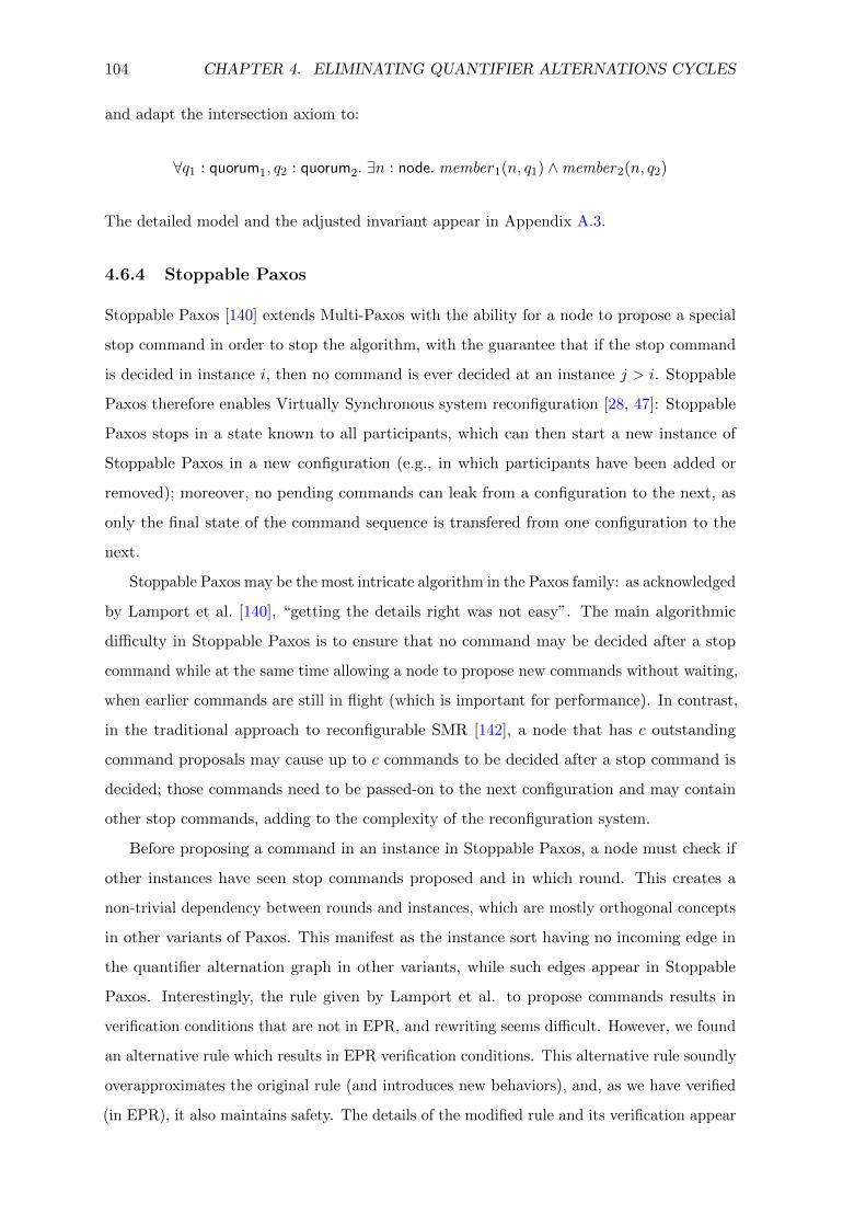
104 CHAPTER 4. ELIMINATING QUANTIFIER ALTERNATIONS CYCLES
and adapt the intersection axiom to:
∀q1 : quorum1, q2 : quorum2. ∃n : node. member1(n, q1) ∧member2(n, q2)
The detailed model and the adjusted invariant appear in Appendix A.3.
4.6.4 Stoppable Paxos
Stoppable Paxos [140] extends Multi-Paxos with the ability for a node to propose a special
stop command in order to stop the algorithm, with the guarantee that if the stop command
is decided in instance i, then no command is ever decided at an instance j > i. Stoppable
Paxos therefore enables Virtually Synchronous system reconfiguration [28, 47]: Stoppable
Paxos stops in a state known to all participants, which can then start a new instance of
Stoppable Paxos in a new configuration (e.g., in which participants have been added or
removed); moreover, no pending commands can leak from a configuration to the next, as
only the final state of the command sequence is transfered from one configuration to the
next.
Stoppable Paxos may be the most intricate algorithm in the Paxos family: as acknowledged
by Lamport et al. [140], “getting the details right was not easy”. The main algorithmic
difficulty in Stoppable Paxos is to ensure that no command may be decided after a stop
command while at the same time allowing a node to propose new commands without waiting,
when earlier commands are still in flight (which is important for performance). In contrast,
in the traditional approach to reconfigurable SMR [142], a node that has c outstanding
command proposals may cause up to c commands to be decided after a stop command is
decided; those commands need to be passed-on to the next configuration and may contain
other stop commands, adding to the complexity of the reconfiguration system.
Before proposing a command in an instance in Stoppable Paxos, a node must check if
other instances have seen stop commands proposed and in which round. This creates a
non-trivial dependency between rounds and instances, which are mostly orthogonal concepts
in other variants of Paxos. This manifest as the instance sort having no incoming edge in
the quantifier alternation graph in other variants, while such edges appear in Stoppable
Paxos. Interestingly, the rule given by Lamport et al. to propose commands results in
verification conditions that are not in EPR, and rewriting seems difficult. However, we found
an alternative rule which results in EPR verification conditions. This alternative rule soundly
overapproximates the original rule (and introduces new behaviors), and, as we have verified
(in EPR), it also maintains safety. The details of the modified rule and its verification appear
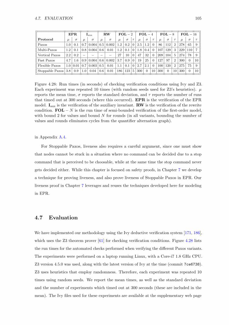
4.7. EVALUATION 105
EPR Iaux RW FOL− 2 FOL− 4 FOL− 8 FOL− 16
Protocol µ σ µ σ µ σ µ σ τ µ σ τ µ σ τ µ σ τ
Paxos 1.0 0.1 0.7 0.004 0.5 0.002 1.2 0.2 0 2.5 1.2 0 86 112 2 278 65 9
Multi-Paxos 1.2 0.1 0.8 0.004 0.6 0.01 1.2 0.1 0 1.8 0.4 0 107 129 3 229 110 7
Vertical Paxos 2.2 0.2 − − − − 27 10 0 47 32 0 209 104 5 274 78 9
Fast Paxos 4.7 1.6 0.9 0.004 0.6 0.002 3.7 0.9 0 19 25 0 127 97 2 300 0 10
Flexible Paxos 1.0 0.01 0.7 0.003 0.5 0.01 1.1 0.1 0 2.7 2.1 0 100 120 2 275 75 9
Stoppable Paxos 3.8 0.9 1.0 0.04 0.6 0.01 186 123 5 300 0 10 300 0 10 300 0 10
Figure 4.28: Run times (in seconds) of checking verification conditions using Ivy and Z3.Each experiment was repeated 10 times (with random seeds used for Z3’s heuristics). µreports the mean time, σ reports the standard deviation, and τ reports the number of runsthat timed out at 300 seconds (where this occurred). EPR is the verification of the EPRmodel. Iaux is the verification of the auxiliary invariant. RW is the verification of the rewritecondition. FOL−N is the run time of semi-bounded verification of the first-order model,with bound 2 for values and bound N for rounds (in all variants, bounding the number ofvalues and rounds eliminates cycles from the quantifier alternation graph).
in Appendix A.4.
For Stoppable Paxos, liveness also requires a careful argument, since one must show
that nodes cannot be stuck in a situation where no command can be decided due to a stop
command that is perceived to be choosable, while at the same time the stop command never
gets decided either. While this chapter is focused on safety proofs, in Chapter 7 we develop
a technique for proving liveness, and also prove liveness of Stoppable Paxos in EPR. Our
liveness proof in Chapter 7 leverages and reuses the techniques developed here for modeling
in EPR.
4.7 Evaluation
We have implemented our methodology using the Ivy deductive verification system [171, 186],
which uses the Z3 theorem prover [61] for checking verification conditions. Figure 4.28 lists
the run times for the automated checks performed when verifying the different Paxos variants.
The experiments were performed on a laptop running Linux, with a Core-i7 1.8 GHz CPU.
Z3 version 4.5.0 was used, along with the latest version of Ivy at the time (commit 7ce6738).
Z3 uses heuristics that employ randomness. Therefore, each experiment was repeated 10
times using random seeds. We report the mean times, as well as the standard deviation
and the number of experiments which timed out at 300 seconds (these are included in the
mean). The Ivy files used for these experiments are available at the supplementary web page
106 CHAPTER 4. ELIMINATING QUANTIFIER ALTERNATIONS CYCLES
of [187]3.
For each Paxos protocol, Figure 4.28 reports the time for checking the inductive invariant
that proves the safety of the EPR model, as well as the times required to verify auxiliary
invariants and rewrite conditions (see Section 4.1.2). We also report on the times required
to check the inductive invariant for the original first-order logic models, using semi-bounded
verification. In all variants, quantifier alternation cycles can be eliminated by bounding the
number of values and rounds. We bound the number of values to 2, and vary the bound on
the number of rounds between 2 and 16 (where most runs time out).
As Figure 4.28 demonstrates, using our methodology for EPR verification results in
verification conditions that are solved by Z3 in a few seconds, with no timeouts, and with
negligible variance among runs with different random seeds. In contrast, when using semi-
bounded verification, the run time quickly increases as we attempt to increase the number of
rounds. Moreover, the variance in run time increases significantly, causing an unpredictable
experience for verification users. We have also attempted to use unbounded verification for
the first-order logic models, but Z3 diverged in this case for all variants. This did not change
when we increased the timeout from 300 seconds to a few hours.
Our empirical results demonstrate that Z3 is stable on EPR formulas, as the performance
has negligible variance when running with different random seeds. This point is one of the
key advantages of EPR for verification, compared to other (undecidable) logics. During the
verification process, one typically runs the verification many times with wrong models or
invariants, as part of the development process. In this process, an unstable solver may fail
unpredictably and without a clear reason. In contrast, our experience with the verification
projects described in this thesis, which is also quantified by the variance data of Figure 4.28,
is that for all practical purposes Z3 performs reliably on EPR formulas. That is, whenever the
verification conditions are in EPR, the solver returns with either a proof or a counterexample.
The solver run time is usually a few seconds, and has a very low sensitivity to random seeds
or other minor perturbations.
Overall, our evaluation demonstrates the practical value of our methodology for EPR
verification, as it allows to transform models whose verification condition cannot be handled
by Z3 (and demonstrate poor scalability and predictability for bounded verification), into
models that can be reliably verified by Z3 in a few seconds.
3http://www.cs.tau.ac.il/~odedp/paxos-made-epr.html

4.8. RELATED WORK FOR CHAPTER 4 107
4.8 Related Work for Chapter 4
Automated verification of distributed protocols Here we review several works that
developed techniques for automated verification of distributed protocols, and compare them
with our approach.
The Consensus Verification Logic CL [69] is a logic tailored to verify consensus algorithms
in the partially synchronous Heard-Of Model [44], with a decidable fragment that can be
used for verification. PSync [70] is a domain-specific programming language and runtime
for developing formally verified implementations of consensus algorithms based on CL and
the Heard-Of Model. Once the user provides inductive invariants and ranking functions in
CL, safety and liveness can be automatically verified. PSync’s verified implementation of
LastVoting (Paxos in the Heard-Of Model) is comparable in performance with state-of-the-art
unverified systems. Compared to these works, our approach tackles a more general setting.
The Heard-Of Model is partially synchronous, while our methodology allowed us to verify
Paxos protocols in the more general asynchronous setting.
Many interesting theoretical decidability results, as well as the ByMC verification tool,
have been developed based on the formalism of Threshold Automata [30, 120–122, 143].
This formalism allows to express a restricted class of distributed algorithms operating in
a partially synchronous communication mode. This restriction allows decidability results
based on cutoff theorems, for both safety and liveness.
A decidable fragment of Presburger arithmetic with function symbols and cardinality
constraint over interpreted sets is developed in [14]. Their work is motivated by applications
to the verification of fault-tolerant distributed algorithms, and they demonstrate automatic
safety verification of some fault-tolerant distributed algorithms expressed in a partially
synchronous round-by-round model similar to PSync.
#Π [231] present a logic that combines reasoning about set cardinalities and universal
quantifiers, along with an invariant synthesis method. The logic is not decidable, so a sound
and incomplete reasoning method is used to check inductive invariants. Inductive invariants
are automatically synthesized by method of Horn constraint solving. The technique is applied
to automatically verify a collection of parameterized systems, including mutual exclusion,
consensus, and garbage collection. However, Paxos-like algorithms are beyond the reach of
this verification methodology since they require more complicated inductive invariants.
Recently, [165] presented a cutoff result for consensus algorithms. They define ConsL, a
domain specific language for consensus algorithms, whose semantics is based on the Heard-Of
Model. ConsL admits a cutoff theorem, i.e., a parameterized algorithm expressed in ConsL

108 CHAPTER 4. ELIMINATING QUANTIFIER ALTERNATIONS CYCLES
is correct (for any number of processors) if and only if it is correct up to some finite bounded
number of processors (e.g., for Paxos the bound is 5) . This theoretical result shows that
for algorithms expressible in ConsL, verification is decidable. However, ConsL is focused
on algorithms for the core consensus problem, and does not support the infinite-state per
process that is needed, e.g., to model Multi-Paxos and SMR.
The above mentioned works obtain automation (and some decidability) by restricting
the programming model. We note that our approach takes a different path to decidability
compared to these works. We axiomatize arithmetic, set cardinalities, and other higher-order
concepts in an uninterpreted first-order abstraction. This is in contrast to the above works,
in which these concepts are baked into specially designed logics and formalisms. Furthermore,
we start with a Turing-complete modeling language and invariants with unrestricted quantifier
alternation, and provide a methodology to reduce quantifier alternation to obtain decidability.
This allows us to employ a general-purpose decidable logic to verify asynchronous Paxos,
Multi-Paxos, and their variants, which are beyond the reach of all of the above works.
Deductive verification in undecidable logic IronFleet [100] is a verified implemen-
tation of SMR, using the Dafny [148] program verifier, with verified safety and liveness
properties. Compared to our work, this system implementation is considerably more detailed.
The verification using Dafny employs Z3 to check verification conditions expressed in unde-
cidable logics that combine multiple theories and quantifier alternations. This leads to great
difficulties due to the unpredictability of the solver. To mitigate some of this unpredictability,
IronFleet adopted a style they call invariant quantifier hiding. This style attempts to specify
the invariants in a way that reduces the quantifiers that are explicitly exposed to the solver.
Our work is motivated by the IronFleet experience and observations. The methodology we
develop provides a more systematic treatment of quantifier alternations, and reduces the
verification conditions to a decidable logic.
Verification using interactive theorem provers Recently, the Coq [26] proof assistant
has been used to develop verified implementations of systems, such as a file system [46], and
shared memory data structures [214]. Closer to our work is Verdi [235, 237], which presents a
verified implementation of an SMR system based on Raft [183], a Paxos-like algorithm. This
approach requires great effort, due to the manual process of the proof; developing a verified
SMR system requires many months of work by verification experts, and proofs measure in
tens of thousands of lines.
In [204, 209] safety of implementations of consensus and SMR algorithms is verified in

4.8. RELATED WORK FOR CHAPTER 4 109
the EventML programming language. EventML interfaces with the Nuprl theorem prover,
in which proofs are conducted, and uses Nuprl’s code generation facilities.
Other works applied interactive theorem proving to verify Paxos protocols at the algo-
rithmic level, without an executable implementation. In [115] correctness of the Disk Paxos
algorithm is proved in Isabelle/HOL, in about 6,500 lines of proof script. Recently, [40]
presented safety proofs of Paxos and Multi-Paxos using the TLA+ [137] specification lan-
guage and the TLA Proof System TLAPS [45]. TLA+ has also been used in Amazon to
model check distributed algorithms [180]. However, they did not spend the effort required to
obtain formal proofs, and only used the TLA+ models for bug finding via the TLA+ model
checker [238].
Compared to our approach, using interactive theorem provers requires more user expertise
and is more labor intensive. We note that part of the difficulty in using an interactive
theorem prover lies in the unpredictability of the automated proof methods available and
the considerable experience needed to write proofs in an idiomatic style that facilitates
automation. An interesting direction of research is to integrate our methodology in an
interactive theorem prover to achieve predictable automation in a style that is natural to
systems designers.
Works based on EPR In [111–113] it was shown that EPR can express a limited form
of transitive closure, in the context of linked lists manipulations, and this was also presented
in Section 3.3. We notice that in the context of the methodology presented in this chapter,
the treatment of transitive closure can be considered as adding a derived relation. Both
works show that EPR is surprisingly powerful, when augmented with derived relations.
In [74], bounded quantifier instantiation is explored as a possible solution to the unde-
cidability caused by quantifier alternations. This work shares some of the motivation and
challenges with our work, but proposes an alternative solution. The context we consider here
is also wider, since we deal not only with quantifier alternations in the inductive invariant, but
also with quantifier alternations in the transition relation. In [74] an interesting connection
is also shown between derived relations and quantifier instantiation, and these insights may
apply to our methodology as well. An appealing future research direction is to combine
user provided derived relations and rewrites together with heuristically generated quantifier
instantiation.
In [219], Ivy is extended beyond what is presented in this thesis to also allow extraction
of verified executable implementations, and verified implementations are developed for both
Multi-Paxos and Raft [183]. The work presented in this thesis has been an enabler for [219],

110 CHAPTER 4. ELIMINATING QUANTIFIER ALTERNATIONS CYCLES
which shows that the techniques we present are general enough to be applied to other
protocols, and to be extended for verifying implementations.

Part II
Invariant Inference
111
Chapter 5
Decidability of Invariant Inference
This chapter is based on the results published in [185].
When using a decidable fragment for modeling transition systems and their invariants,
checking if an invariant is inductive is decidable. It is therefore natural to investigate the
decidability of the problem of invariant inference, i.e., the problem of finding a suitable
inductive invariant for proving that a given system satisfies a given safety property. This
problem is parameterized by a language (i.e., infinite set of first-order sentences) L, the
search space of potential inductive invariants. This chapter explores this problem in a
general context, develops restrictions under which this problem is decidable, and also obtains
undecidability results that show the restrictions are necessary.
Many techniques attempt to mechanize the search for inductive invariants. Such tools
are only able to infer inductive invariants in a certain language, and are hence necessarily
incomplete in verifying safety. Their output may be: (i) program is safe (found inductive
invariant); or (ii) program is unsafe (found a concrete counterexample); or (iii) don’t know or
diverge. Since the safety verification problem is undecidable, this incompleteness is expected
and therefore mostly accepted by users of such techniques. However, since actual tools search
for inductive invariants in a certain language, the underlying decision problem they address
is in fact “is there an inductive invariant in a certain language?” A key observation is that
this problem is different from the safety verification problem, and hence might be decidable
even in cases where safety verification is not.
This chapter investigates the decidability of the problem of inferring inductive invariants
in a given language. Here, the expected outcome is not “safe/unsafe”, but rather “inductive
invariant exists/does not exist in the given language”. Investigating the decidability of this
problem is important to better understand the foundation of existing methods for invariant
112

113
inference (e.g., abstract interpretation [56, 57], IC3/PDR [34, 116]): whenever the problem
is undecidable, no tool will be able to be complete even for the language in which it is
searching; in contrast, when the problem is decidable, tool developers can aim to have
complete algorithms for a restricted language.
This chapter formulates the general problem of inferring inductive invariants in a restricted
language L (Section 5.2), and applies the technique of [5–7, 9, 76] based on well-quasi-orders
(wqo’s) to get sufficient conditions for decidability of invariant inference (Section 5.3). The
formalization is parametric in the language L, and associates with each language L a quasi-
order vL on the state space, such that if vL is a wqo, then invariant inference in L is
decidable. This leads to a (parametric) connection between transition systems specified
in first-order logic, first-order languages, and the decidability technique based on wqo’s
(Section 5.4). This connection is the basis for the following main results of this chapter.
Decidability of universal invariants for deterministic paths We prove (Section 5.5)
that for programs manipulating graphs with outdegree one, modeled in EPR as discussed
in Section 3.3, and restricting to universally quantified inductive invariants, the invariant
inference problem is decidable (while safety is still undecidable). This class includes many
programs manipulating singly-linked-lists [112]. The technical proof builds on Kruskal’s Tree
Theorem [129] to show that the suitable vL is a wqo, as it corresponds to homeomorphic
embedding of graphs. Being formulated in logic, this result naturally extends to capture
programs with additional structure beyond graph reachability (e.g., sorting algorithms for
linked lists). The complexity of inferring universally quantified invariants even for linked-list
programs is shown to be non-elementary (Section 5.7.4).
Undecidability of alternation-free invariants for deterministic paths We show
(Section 5.7.2) that in the same setting as above, inferring alternation-free invariants is
undecidable. Namely, mixing universal and existential information even without alternation
makes invariant inference undecidable. This demonstrates that the invariant inference
problem is theoretically harder than invariant checking, since in this setting checking
inductiveness of an alternation-free invariant is decidable. This also shows that in this setting
the restriction to universal invariants is necessary for decidability of invariant inference.
Undecidability of universal invariants for general systems Modeling systems be-
yond deterministic paths (or linked-lists) requires additional unrestricted relations. However,
we show (Section 5.7.3) that in the presence of a single unrestricted binary relation, invariant

114 CHAPTER 5. DECIDABILITY OF INVARIANT INFERENCE
x := 1
y := 2
while *:
assert x > 0
x := x + y
y := y + 1
Figure 5.1: A simple loop example.
inference is undecidable even when restricting to universal invariants. This is done by
constructing a safe transition system that has a universal inductive invariant if and only if a
given counter machine halts.
New decidability from old: systematic constructions for decidability To over-
come the general undecidability while allowing unrestricted relations, we provide (Section 5.6)
systematic ways to construct classes of systems and languages for invariants for which invari-
ant inference is decidable. These constructions start with some established wqo, (e.g., the
deterministic paths class with universal invariants) and gradually extend it to construct new
systems with suitable wqo’s. This process results in systems richer than the original one,
while decidability is maintained by further restricting the language of potential invariants. We
demonstrate the constructions by obtaining a decidable fragment of the invariant inference
problem that captures a nontrivial example of a network learning switch.
5.1 Overview
This section provides a short overview of the problem addressed in this chapter and the main
results.
5.1.1 Motivation and Background
Inductive invariants can be difficult to find both manually and using automatic program
analysis. This was discussed in Section 1.2 and identified as Challenge 2, and here we
elaborate further to motivate the investigation of this chapter.
Consider the example listed in Figure 5.1, of a simple loop, with the safety property
P = x > 0.1 The program executes the loop for an unbounded number of iterations, starting
from a state where x = 1 and y = 2. Clearly, x < 1000 for example is not an invariant at
all in this program, since it is violated after 500 loop iterations. Interestingly, the required
1We note that this work does not consider numeric domains, but it is useful to illustrate the notion ofinductive invariants using a simple numeric program.
5.1. OVERVIEW 115
safety property P = x > 0 is invariant in this program but it is not an inductive invariant.
For example, if we execute the loop body in a state in which y is negative, it will be violated.
In order to come up with an inductive invariant, we need to also prove something about y.
For example, x > 0∧ y ≥ 2 and x > 0∧ y > 0 are both inductive invariants that prove P for
this program. However, if we restrict the language of inductive invariants to consider x only,
i.e., to a language whose formulas are not allowed to mention y, then no inductive invariant
for P exists for this program.
Inferring inductive invariants in a restricted language This chapter addresses the
decision problem that corresponds to inductive invariant inference, defined as follows:
Given a transition system T = (Σ,Γ, ι, τ), a safety property P , and a (usually
infinite) family of candidate invariants L: does there exist a formula in L that is
an inductive invariant for (T, P )?
Notice that this problem is relevant for abstract interpretation [56, 57], since L can be viewed
as an abstract domain, in which case this question amounts to asking if the abstract domain
is precise enough for the given program and property. Also notice that in reality one is
interested in algorithms for this problem, which are not considered in this thesis. Finally,
we note that if L is a finite set and if invariant checking is decidable, then the problem of
inferring inductive invariants is trivially decidable.
Working with a restricted language of potential invariants L is beneficial in many
situations, as it may lead to decidability both of invariant checking, and of invariant inference.
Additionally, we note that a negative answer to the invariant inference problem of the form:
“There exists no inductive invariant in L which can be used to verify that your program
satisfies P” can be useful for programmers. The programmer may decide to simplify their
program such that there will be an inductive invariant in L. To facilitate this, the verifier
should also provide a clear explanation as to why there is no inductive invariant in the
restricted language. In this case, such an answer is significantly better than an inconclusive
alarm of the form: “Your program may not satisfy P”, which even the most sophisticated
static analysis tools sometimes provide.
Decidability via well-quasi-orders To address the decidability of inferring inductive
invariants in a restricted language L, we apply the technique of [5–7] based on well-quasi-
orders (wqo’s).
The set of potential inductive invariants L naturally defines the following quasi-order on

116 CHAPTER 5. DECIDABILITY OF INVARIANT INFERENCE
states (models):
s vL s′ iff ∀ϕ ∈ L. s′ |= ϕ ⇒ s |= ϕ (5.2)
Thus, smaller or lower states according to vL satisfy more formulas from L. Notice that
this is a quasi-order, i.e., it is reflexive and transitive. Whenever vL is a well-quasi-order
(wqo), that is, any infinite sequence s0, s1, . . ., contains an increasing pair si vL sj with i < j,
then invariant inference in L is decidable (provided some natural effectiveness assumptions).
Intuitively, invariant inference in L can be done by backward reachability analysis (which
can be seen as iterative application of Dijkstra’s weakest precondition). The fact that vL is
a wqo guarantees the termination of this process.
Universal invariants A natural and useful language for inductive invariants is the set of
universally quantified sentences, or universal invariants. Universal invariants can be used to
prove properties of many infinite-state systems, e.g., parameterized systems and programs
with unbounded heap allocation or unbounded arrays. The universal quantification is usually
over all nodes in a network, or all the elements in the heap or the array (e.g., [208] for heaps
and [59, 193] for arrays). Furthermore, linked-lists can be formulated using a theory of
list reachability which allows deciding inductiveness of universal invariants using effectively
proportional logic (EPR) [112]. When L is the set of all universal sentences, we denote the
quasi-order of Equation (5.2) by v∀∗ . We note that v∀∗ is the substructure relation known
from model theory (e.g., [42]). That is, s v∀∗ s′ iff s is isomorphic to a substructure of s′.
5.1.2 Decidability of Inferring Universal Invariants for Deterministic
Paths
When using the encoding presented in Section 3.3 to model reachability in graphs of outdegree
one, we prove that the structures that arise are well-quasi-ordered by the substructure relation.
This leads to decidability of inferring universal invariants for programs manipulating such
graphs, including many programs manipulating singly-linked-lists [112]. The proof utilizes
Kruskal’s Tree Theorem [129], and relates homeomorphic embedding of trees with the
substructure relation. The proof using Kruskal’s Tree Theorem naturally supports adding
any finite number of unary relations, which denote sets of individuals, while still maintaining
decidability of invariant inference. This allows adding unary instrumentation relations, which
is useful for example in verifying sorting implementations [151].

5.1. OVERVIEW 117
5.1.3 Undecidability and Complexity of Invariant Inference
A natural way to extend universal invariants is by allowing Boolean combinations of universal
invariants and existential invariants. These are called alternation-free invariants since they
forbid alternating universal and existential quantifiers. In [112], it was shown that this class
of invariants suffices to prove partial correctness of many linked-list manipulating programs.
Moreover, checking inductiveness of alternation-free invariants is still decidable in EPR.
While checking inductiveness is still decidable, we show that the invariant inference
problem is undecidable for alternation-free invariants. This is proven by a reduction from
the halting problem of counter machines: given a counter machine we construct a program
and property such that the counter machine terminates in k steps if and only if there exists
an inductive invariant with O(k) quantifiers for the program. While this result is somehow
expected given the unbounded nature of quantified invariants and the complexity of inductive
reasoning, we note that it differs from the standard reductions (e.g., [32]) that show that the
safety problem for certain classes of programs is undecidable, as our constructed program is
safe whether the counter machine halts or not. This result shows an interesting case where
invariant inference is undecidable while invariant checking is decidable.
The undecidability result implies that for linked-list manipulating programs, restricting
to universal invariants is necessary for the decidability of invariant inference. By using a
similar reduction, we also show that inferring universal invariants for linked-list programs
has non-primitive complexity. This reduction is from the safety problem of lossy counter
machines: given a lossy counter machine, we construct a program such that the program has
a universal inductive invariant iff the lossy counter machine is safe.
For modeling systems beyond linked-lists, additional unrestricted relations are needed.
However, we show that even when restricting to universal invariants, invariant inference
becomes undecidable in the presence of a single unrestricted binary relation. We do this by
a similar reduction from the halting problem of counter machines. As before, we construct a
system that has a universal invariant with O(k) quantifiers iff a given counter machine halts
in k steps. This shows that for many general systems beyond linked-lists, inferring universal
invariants is undecidable.
5.1.4 Systematic Constructions for Decidability
The most exciting part of the work presented in this chapter is the ability to show that it is
decidable to infer restricted universal invariants in many parametric systems. We note that
despite their inherent limitations, universal invariants can be used to model many aspects

118 CHAPTER 5. DECIDABILITY OF INVARIANT INFERENCE
of systems by using uninterpreted relations. However, as noted above, for the language
of all universal invariants, even one unrestricted binary relation makes invariant inference
undecidable. To obtain decidability, we further restrict the language of potential universal
invariants. To do so, we start from an already established “base” wqo (e.g., the deterministic
paths class with universal invariants), and present systematic constructions that extend
classes of systems and languages for invariants in a limited way to construct new systems for
which vL is a wqo by construction, and thus invariant inference is decidable (see Section 5.6).
The resulting languages are subsets of the set of all universal invariants.
Symmetric lifting We show that a decidability result for some class of programs and
language which relies on an underlying theory (e.g., deterministic paths) can be lifted to
systems that are modeled by an unbounded number of instances of the theory, by creating a
language of restricted universal sentences that do not correlate the different instances. We
call this operation symmetric lifting, and it can be used to model systems beyond linked-lists
and deterministic paths by using high-arity relations. For example, the routing tables in
a network of switches may be modeled by a ternary relation route, where route(d,m, n)
denotes that messages sent to destination d which arrive at switch m will be forwarded to
n. Essentially, the routing tables can be viewed as an unbounded number of graphs with
outdegree one — one graph for each destination d. In many cases the invariants do not need
to correlate the different instances of the original theory (e.g., it is unnecessary to relate
the routing tables for different destinations). For such cases, we show that an established
wqo (e.g., that of deterministic paths) can be lifted to obtain a wqo for a system where the
relations have an increased arity, which corresponds to an unbounded number of instances
of the base theory. The fact that wqo’s are preserved by symmetric lifting is proved using
Higman’s Lemma [104].
Bounded occurrences of unrestricted relations It is sometimes necessary for the
invariant to mention unrestricted relations (i.e., relations that do not obey any background
theory). For example, a model of a distributed protocol such as a learning switch may
use a relation msg of arity 4, where msg(s, d,m, n) denotes that a packet with source s
and destination d is pending on the link from n to m. Moreover, the invariant might need
to relate the msg relation to reachability information such as forwarding paths stored in
the route relation mentioned above. To handle such cases, we show that wqo and thus
decidability of invariant inference is preserved by extending a language of universal invariants
to include unrestricted relations, as long as only a bounded number of occurrences of these

5.2. THE INDUCTIVE INVARIANT INFERENCE PROBLEM 119
relations appear in each universal clause. For the case of the learning switch, adding one
such occurrence suffices to obtain an inductive invariant.
This extension is not trivial since the occurrences of the unrestricted relations are allowed
to create correlations with relations that may appear an unbounded number of times under
an unbounded number of quantifiers (e.g., to correlate msg and route). For this reason, this
result cannot be obtained as a straightforward cartesian product with a finite domain, and
the proof also relies on Higman’s Lemma to show that the wqo is preserved.
5.2 The Inductive Invariant Inference Problem
In this section we formalize the inductive invariant decision problem parameterized by the
language of invariants, and contrast it with the classical safety decision problem. The basic
definitions used here are those of Section 2.3 for a transition system T = (S, S0, R), a safety
property P ⊆ S, an inductive invariant I ⊆ S, and a CTI (counterexample to induction)
s ∈ S. In this chapter, a transition system will always have an associated safety property,
so by overloading of terminology, we will also use transition system to mean a transition
system and a safety property: (S, S0, R, P ).
Classes of transition systems and properties We are interested in formulating decision
problems where the input consists of a transition system and a safety property. In the
following sections we investigate decidability of these problems for various classes of transition
systems and safety properties, where the class is understood to define an effective way to
represent its transition systems and safety properties. We use C to denote such a class. For
example, one could define the class of digital circuits, where the state space is given by
the valuation of Boolean variables, and the set of initial states, the transition relation, and
the safety property are described using propositional formulas. Another example is that of
programs in some programming language, where the safety property might be defined via
assertions within the program. Our focus will be of course classes of first-order transition
systems, as defined in Section 2.4, but we start with a general mindset. We write (T, P ) ∈ Cto denote that (T, P ) is an instance of class C.
The safety decision problem The classical problem of determining the safety of a
transition system taken from a given class C of transition systems can be formulated as the

120 CHAPTER 5. DECIDABILITY OF INVARIANT INFERENCE
following decision problem:
SAFE[C] = {(T, P ) ∈ C | T |= P}
Recall that for many classes of infinite-state transition systems, SAFE[C] is undecidable
(as T can encode a Turing machine).
Languages for expressing inductive invariants We are interested in deciding whether
a given transition system (including a safety property) has an inductive invariant which is
expressible in a given language. Therefore, the input to the inductive invariant inference
problem is a transition system with a safety property, (T, P ), and a language L ⊆ P (S)
(where S is the set of states of T ) that determines the inductive invariants of interest. As
such, the inductive invariant problem is defined not only with respect to a class C of transition
systems (and properties), but also with respect to a class L of languages.
For example, if C is the class of digital circuits represented by propositional formulas
over Boolean variables, then L might restrict to languages L that contain sets expressible by
propositional formulas over some of the variables. In this case, if the formulas can mention
all the propositional variables, then every set of states is in L. On the other hand, if C is the
class of transition systems specified in first-order logic, and L restricts to languages L that
contain sets expressible by quantifier free formulas (or universal formulas), then some sets of
states might not be in L. Since the definition of L might depend on C, we consider them as
a pair (C,L). We write (T, P, L) ∈ (C,L) to denote that (T, P, L) is an instance of (C,L).
We say that a set A ⊆ S is expressible in L if A ∈ L.
The inductive invariant inference problem Given C and L, we define the decision
problem INV[C,L] as follows: given a transition system, T = (S, S0, R), a safety property, P ,
and a language, L ⊆ P (S), such that (T, P, L) ∈ (C,L), is there an inductive invariant for
(T, P ) which is expressible in L. Formally:
INV[C,L] = {(T, P, L) ∈ (C,L) | ∃I ∈ L s.t. I is an inductive invariant for (T, P )}
Note that for every C and L, if (T, P, L) ∈ INV[C,L] then (T, P ) ∈ SAFE[C]. That is,
if there exists an inductive invariant (in L) for a transition system then it is safe. The
converse does not necessarily hold, and there could be cases where (T, P ) ∈ SAFE[C] but
(T, P, L) 6∈ INV[C,L]. This can happen if the language L is not expressive enough to describe
5.3. SUFFICIENT CONDITIONS FOR DECIDABILITY OF INV[C,L] 121
an inductive invariant for (T, P ). This suggests that INV[C,L] may be decidable even if
SAFE[C] is undecidable.
Also note that decidability issues are of interest when C allows the definition of an infinite
set of states and L allows the definition of infinitely many sets, since in the finite case both
SAFE[C] and INV[C,L] can be decided by a naive enumeration. This is the case, for example,
for the class of digital circuits with invariants expressed as propositional formulas.
Effectiveness assumptions In this chapter we restrict our attention to classes C and Lsuch that the following effectiveness assumptions hold:
(i) there is a decision procedure that, given (T, P, L) ∈ (C,L), determines membership in
S, S0, R, P , and L,
(ii) there is a decision procedure that checks, given (T, P, L) ∈ (C,L) and a set I ∈ L,
whether I is an inductive invariant for (T, P ), and provides s ∈ S, a CTI (coun-
terexample to induction) for I, if it is not (see Section 2.3 for the definition of a
CTI).
Note that as C and L are used to define decision problems, they come with a finite
encoding of their instances, and the set of instances of (C,L) is also assumed to be decidable.
5.3 Sufficient Conditions for Decidability of INV[C,L]
In this section, we apply the technique of [5–7, 9] based on well-quasi-orders (wqo’s) to obtain
sufficient conditions for the decidability of INV[C,L]. To do so, for (T, P, L) ∈ (C,L), we
define a quasi-order, denoted vL, on the states of the transition system T . The quasi-order
vL has the property that if it is a well-quasi-order for any (T, P, L) ∈ (C,L), and if (C,L)
has several other simple properties, then INV[C,L] is decidable.
Well-founded sets and well-quasi-orders We first recall the definitions of a well-quasi-
order (wqo) and a well-founded set. Let (X,≤) be a quasi-order, i.e., ≤ is reflexive and
transitive. We say that (X,≤) is well-founded if it does not contain any infinite strictly
decreasing chain x0 > x1 > . . .. We say that the infinite sequence x0, x1, . . . is an antichain
if every two elements in it are incomparable, i.e., xi 6≤ xj for all i 6= j. We say that (X,≤) is
a well-quasi-order (wqo) [130] if for every infinite sequence of elements x0, x1, . . . there exists
i < j such that xi ≤ xj . Equivalently, (X,≤) is a wqo if (X,≤) is well-founded and does not
contain antichains.

122 CHAPTER 5. DECIDABILITY OF INVARIANT INFERENCE
5.3.1 Quasi-Order and Exclusion Operator for L
We now present several definitions, parameterized by a language for potential inductive
invariants.
Definition 5.3 (vL). For any language L ⊆ P (S), we define a quasi-order vL on S given
by
s1 vL s2 iff for all A ∈ L : s2 ∈ A implies s1 ∈ A
Thinking of A as an L-property, s1 vL s2 says that every L-property satisfied by s2 is
satisfied by s1. That is, s1 satisfies more (or the same) L-properties than s2.
Definition 5.4 (AvoidL). Let s ∈ S be a state and let A ∈ L be a set such that s 6∈ A, and
for every A′ ∈ L, if s 6∈ A′ then A′ ⊆ A. Then we denote A by AvoidL(s).
That is, AvoidL(s) is the maximum (w.r.t. set inclusion) over all sets in L that do not
include s. Note that AvoidL(s) need not exist. However, if it exists, it is unique and equal
to the union of all sets in L that do not include s. AvoidL(s) and vL are strongly related:
Lemma 5.5. For all s, s′ such that AvoidL(s) exists, s vL s′ iff s′ 6∈ AvoidL(s).
Proof. The “only-if” direction directly follows from the definitions. For the “if” direction,
assume s 6vL s′. Then there exists A ∈ L such that s′ ∈ A, but s 6∈ A. The latter implies
A ⊆ AvoidL(s) and thus, s′ ∈ AvoidL(s).
5.3.2 L-Relaxed Transition System & Decidability of INV[C,L]
In this section, we formulate sufficient conditions for decidability of INV[C,L]. Given
(C,L), we say that AvoidL is computable in (C,L) if there exists a procedure that, given
(T, P, L) ∈ (C,L) and s ∈ S, computes AvoidL(s). (In particular, this implies that AvoidL(s)
exists for every s ∈ S.)
Theorem 5.6. Let (C,L) be such that:
(i) for every (T, P, L) ∈ (C,L), L is closed under finite intersections;
(ii) AvoidL is computable in (C,L); and
(iii) for every (T, P, L) ∈ (C,L), where T = (S, S0, R), (S,vL) is a wqo.
Then INV[C,L] is decidable. Furthermore, Algorithm 5.1 is a decision procedure for it.
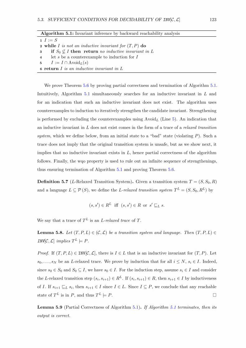
5.3. SUFFICIENT CONDITIONS FOR DECIDABILITY OF INV[C,L] 123
Algorithm 5.1: Invariant inference by backward reachability analysis
1 I := S2 while I is not an inductive invariant for (T, P ) do3 if S0 6⊆ I then return no inductive invariant in L4 let s be a counterexample to induction for I5 I := I ∩AvoidL(s)
6 return I is an inductive invariant in L
We prove Theorem 5.6 by proving partial correctness and termination of Algorithm 5.1.
Intuitively, Algorithm 5.1 simultaneously searches for an inductive invariant in L and
for an indication that such an inductive invariant does not exist. The algorithm uses
counterexamples to induction to iteratively strengthen the candidate invariant. Strengthening
is performed by excluding the counterexamples using AvoidL (Line 5). An indication that
an inductive invariant in L does not exist comes in the form of a trace of a relaxed transition
system, which we define below, from an initial state to a “bad” state (violating P ). Such a
trace does not imply that the original transition system is unsafe, but as we show next, it
implies that no inductive invariant exists in L, hence partial correctness of the algorithm
follows. Finally, the wqo property is used to rule out an infinite sequence of strengthenings,
thus ensuring termination of Algorithm 5.1 and proving Theorem 5.6.
Definition 5.7 (L-Relaxed Transition System). Given a transition system T = (S, S0, R)
and a language L ⊆ P (S), we define the L-relaxed transition system TL = (S, S0, RL) by
(s, s′) ∈ RL iff (s, s′) ∈ R or s′ vL s.
We say that a trace of TL is an L-relaxed trace of T .
Lemma 5.8. Let (T, P, L) ∈ (C,L) be a transition system and language. Then (T, P, L) ∈INV[C,L] implies TL |= P .
Proof. If (T, P, L) ∈ INV[C,L], there is I ∈ L that is an inductive invariant for (T, P ). Let
s0, . . . , sN be an L-relaxed trace. We prove by induction that for all i ≤ N , si ∈ I. Indeed,
since s0 ∈ S0 and S0 ⊆ I, we have s0 ∈ I. For the induction step, assume si ∈ I and consider
the L-relaxed transition step (si, si+1) ∈ RL. If (si, si+1) ∈ R, then si+1 ∈ I by inductiveness
of I. If si+1 vL si, then si+1 ∈ I since I ∈ L. Since I ⊆ P , we conclude that any reachable
state of TL is in P , and thus TL |= P .
Lemma 5.9 (Partial Correctness of Algorithm 5.1). If Algorithm 5.1 terminates, then its
output is correct.

124 CHAPTER 5. DECIDABILITY OF INVARIANT INFERENCE
Proof. If Algorithm 5.1 determines that I is an inductive invariant, correctness follows from
the loop condition. For the case where Algorithm 5.1 determines that no inductive invariant
exists in L, we prove by induction on the loop iterations of Algorithm 5.1 that for every
state s′ 6∈ I, there exists an L-relaxed trace of T leading from s′ to some state 6∈ P . Hence,
if S0 6⊆ I, it follows that TL 6|= P , and by Lemma 5.8, (T, P, L) 6∈ INV[C,L]. The base case
of the induction is trivial (initially I = S). For the induction step, let s′ be a state that is
removed from I since it is not in AvoidL(s). By the definition of a CTI (Section 2.3), either
s 6∈ P or there exists s′′ 6∈ I such that (s, s′′) ∈ R. By the induction hypothesis for I, we get
that in both cases, s itself has an L-relaxed trace leading to some state 6∈ P . By Lemma 5.5,
s vL s′, so s′ also has an L-relaxed trace leading to a state 6∈ P .
In the general case, Algorithm 5.1 is not guaranteed to terminate. However, the following
lemma gives a natural condition for its termination.
Lemma 5.10 (Termination of Algorithm 5.1). If (L,⊆) is well-founded, then Algorithm 5.1
always terminates.
Proof. For i ≥ 0, let Ii denote the set I at the i’th loop iteration of Algorithm 5.1. The
sequence I0, I1, . . . is strictly decreasing with respect to set inclusion, so it must be finite by
well-foundedness.
The proof Theorem 5.6 is completed by the following lemma.
Lemma 5.11. Let L ⊆ P (S) be a language such that (S,vL) is a wqo, then (L,⊆) is
well-founded.
Proof. Assume to the contrary that there exists a strictly decreasing infinite sequence
A0 ⊃ A1 ⊃ A2 . . . of sets in L. For every i ≥ 0 let si be a state in Ai \ Ai+1. For every
i < j, Aj ⊆ Ai+1, and therefore si 6∈ Aj . Hence, for every i < j, Aj ∈ L and sj ∈ Aj but
si 6∈ Aj . This implies that si 6vL sj for every i < j, in contradiction to the fact that (S,vL)
is a wqo.
In fact, the correctness proof of Algorithm 5.1 also provides the following corollary, which
is the converse of Lemma 5.8 under the conditions of Theorem 5.6. This will become useful
in Section 5.7.4.
Corollary 5.12. Let (C,L) be such that: (i) for every (T, P, L) ∈ (C,L), L is closed under
finite intersections; (ii) AvoidL is computable in (C,L); and (iii) for every (T, P, L) ∈ (C,L),
where T = (S, S0, R), (S,vL) is a wqo. Then (T, P ) ∈ INV[C,L] if and only if TL |= P .

5.4. EPR CLASSES OF TRANSITION SYSTEMS AND INVARIANTS 125
Proof. If TL |= P , then a L-relaxed trace leading from an initial state to a state 6∈ P does
not exist. By the proof of Lemma 5.9, this implies that Algorithm 5.1 does not terminate in
Line 3. Thus, it necessarily finds an inductive invariant.
5.4 EPR Classes of Transition Systems and Invariants
In the rest of this chapter we focus on classes of transition systems, safety properties, and
languages of inductive invariants that are expressed in first-order logic, and specifically in
EPR. This section provides the necessary formal definitions of these classes, building on the
formalism of Section 2.4 to represent transition systems, safety properties, and inductive
invariants using formulas in first-order logic.
5.4.1 Classes of Transition Systems and Properties
For the rest of this chapter, we will be interested in classes of transition systems and properties
that are subsets of the class of EPR transition systems, defined below. For simplicity of
the presentation, in this chapter we use the relational unsorted EPR fragment, i.e., the
vocabulary contains a single sort and no function symbols.2
Definition 5.13 (CEPR). The class CEPR, of EPR transition systems contains transition
systems and properties (T, P ), where T = (Σ,Γ, ι, τ), such that Σ contains only relation and
constant symbols (i.e., no function symbols), Γ is a finite set of ∃∗∀∗ formulas (i.e., formulas
whose prenex normal form has quantifier prefix ∃∗∀∗) over Σ, and the formulas ι, τ , and ¬Pare also ∃∗∀∗ formulas.
As mentioned in Section 5.2, a class is expected to provide an effective encoding of sets
of states (e.g., initial states, transitions), and for CEPR such sets are represented by formulas.
A class is also expected to provide an efficient encoding of individual states in the state
space of its transition systems. To accomplish this for CEPR, in this chapter we use the finite
structure semantics, defined in Section 2.4.3. This means that the states of a transition
system are only the finite structures over Σ that satisfy Γ. Finite structures can clearly be
effectively encoded. Note that in this chapter we are only interested in safety properties, and
only under restrictions that ensure that all verification conditions are in EPR, which has the
finite model property. Thus, as also explained in Section 2.4.3, the distinction between the
finite structure semantics and the first-order semantics is immaterial, and the results hold in
both semantics.2This restriction in not detrimental since functions can be represented as relations of increased arity.
However, such an encoding loses the fact that relations representing functions are total.

126 CHAPTER 5. DECIDABILITY OF INVARIANT INFERENCE
In the rest of this chapter, we use STRUCT[Σ] to denote the set of finite structures over
Σ, and STRUCT[Σ,Γ] to denote the set of finite structures over Σ that satisfy Γ. Thus, for
an EPR transition system T = (Σ,Γ, ι, τ), the state space is STRUCT[Σ,Γ].
5.4.2 Languages of Inductive Invariants
As we consider classes of transition systems expressed in EPR, we also wish to express
inductive invariants as formulas in first-order logic, such that the verification conditions for
checking inductiveness (see Section 2.4.2) are in EPR. We focus on the two classes defined
below (and subclasses thereof to be defined later).
Definition 5.14 (L∀∗). The L∀∗ class of languages restricts invariants to closed universal
formulas (i.e., formulas with a ∀∗ quantifier prefix). Each vocabulary Σ induces another
language of class L∀∗ . Since Σ is typically clear from the context, we omit it from the
notation, and simply write ∀∗ to denote a language from L∀∗ , i.e., the set of universally
quantified formulas over some vocabulary.
Definition 5.15 (LAF). The LAF class of languages restricts invariants to alternation-free
formulas. These are formulas obtained by conjunctions and disjunctions of closed universal
formulas (with ∀∗ quantifier prefix) and closed existential formulas (with ∃∗ quantifier prefix).
Effectiveness assumptions in EPR For classes that are subclasses of CEPR and LAF
(in particular, including L∀∗ ⊆ LAF), effectiveness assumption (i) formulated in Section 5.2
corresponds to decidability of checking whether a given structure satisfies a formula, and
effectiveness assumption (ii) corresponds to decidability of satisfiability of the verification
conditions (as formalized in Section 2.4.2). Since all verification conditions are in EPR,
checking their satisfiability is decidable, and moreover, produces a finite structure as a CTI
if the invariant is not inductive. Therefore, all the effectiveness requirements are satisfied for
any C′ ⊆ CEPR and L′ ⊆ LAF. Also observe that the finite model property of the verification
conditions means that the set INV[C′,L′] is the same regardless of whether we interpret its
definition under the finite structure semantics or the first-order semantics.
5.4.3 vL and AvoidL in EPR
Finally, we state the first-order logic and EPR realization of the definitions of vL and
AvoidL(s), which are used to formulate the sufficient conditions for decidability in Theo-
rem 5.6.

5.4. EPR CLASSES OF TRANSITION SYSTEMS AND INVARIANTS 127
In the first-order formalism, the state space is STRUCT[Σ,Γ], and a language L of
potential inductive invariants is a set of first-order formulas (each of which represents a
set of states). In this setting, s1 vL s2 iff for all ϕ ∈ L, s2 |= ϕ implies s1 |= ϕ. Similarly,
AvoidL(s) is the weakest formula ϕ ∈ L such that s 6|= ϕ. That is, s 6|= AvoidL(s), and for
every ϕ ∈ L, if s 6|= ϕ then Γ, ϕ |= AvoidL(s).
We note that for first-order languages, requirement i of Theorem 5.6 corresponds to
closure of L under (finite) conjunctions. This property holds for all languages we consider.
The theorem also requires computability of AvoidL (requirement ii). Next, we show that
this requirement holds for (CEPR,L∀∗) and subclasses thereof.
Computability of Avoid∀∗ for EPR classes To show that Avoid∀∗ is computable, we
show that v∀∗ and Avoid∀∗ are closely related to the model theoretic notions of substructure
and diagram, which are themselves closely related (see e.g., [42]).
Definition 5.16 (Diagram). Let s = (D, I) be a finite structure over Σ and let D =
{e1, . . . , e|D|}. The diagram of s, denoted by Diag(s), is the following formula over Σ:
∃x1 . . . x|D|. distinct(x1, . . . , x|D|) ∧ ψ
where distinct(x1, . . . , xn) =∧
1≤i<j≤n xi 6= xj , and ψ is the conjunction of:
• xi = c for every constant symbol c such that I(c) = ei;
• r(xi1 , . . . , xik) for any relation r of arity k in Σ and any i1, . . . , ik s.t.
(ei1 , . . . , eik) ∈ I(r); and
• ¬r(xi1 , . . . , xik) for any relation r of arity k in Σ and any i1, . . . , ik s.t.
(ei1 , . . . , eik) 6∈ I(r).
Intuitively, one can think of Diag(s) as the formula produced by treating individuals in
D as existentially quantified variables and explicitly encoding the interpretation of every
constant and every relation symbol. Clearly, s |= Diag(s). Recall that s1 = (D1, I1) is a
substructure of s2 = (D2, I2) if D1 ⊆ D2 and for every a ∈ Σ, I1(a) is the restriction of I2(a)
to D1. It is well known (e.g., [42]) that s2 |= Diag(s1) iff s1 is isomorphic to a substructure
of s2. Moreover, for every closed existential formula ϕ over Σ, s |= ϕ iff Diag(s) |= ϕ. This
immediately implies the following two lemmas.
Lemma 5.17. s1 v∀∗ s2 iff s1 is isomorphic to a substructure of s2.

128 CHAPTER 5. DECIDABILITY OF INVARIANT INFERENCE
Proof. Suppose s1 v∀∗ s2. Recall that s1 v∀∗ s2 iff s1 satisfies all the universal formulas that
are satisfied by s2. s1 |= Diag(s1) so s1 6|= ¬Diag(s1), hence s2 6|= ¬Diag(s1) (as s1 v∀∗ s2
and ¬Diag(s1) ∈ ∀∗), so, s2 |= Diag(s1), and s1 is isomorphic to a substructure of s2.
For the converse, suppose s1 is isomorphic to a substructure of s2. Then s2 |= Diag(s1),
and therefore Diag(s2) |= Diag(s1). To see that s1 v∀∗ s2, consider ϕ ∈ ∀∗ such that s2 |= ϕ.
Assume to the contrary that s1 6|= ϕ, i.e., s1 |= ¬ϕ, hence Diag(s1) |= ¬ϕ, which implies
that Diag(s2) |= ¬ϕ, i.e. s2 |= ¬ϕ, which provides a contradiction.
So, for finite structures, v∀∗ is the same as the substructure relation (up to isomorphism).
Lemma 5.18. For every s = (D, I), Avoid∀∗(s) is given by the prenex normal form of
¬Diag(s). In particular, it is computable.
Proof. First, s 6|= ¬Diag(s) since s |= Diag(s). In addition, let ϕ ∈ ∀∗ be such that s 6|= ϕ.
Then s |= ¬ϕ (where ¬ϕ is existential), hence Diag(s) |= ¬ϕ, so ϕ |= ¬Diag(s) as needed.
With this, we have shown that requirements i and ii of Theorem 5.6 are easily satisfied
by (CEPR,L∀∗) and subclasses thereof. The more difficult and interesting requirement is
of course requirement iii, namely that vL is a wqo. This requirement will be our focus in
Sections 5.5 and 5.6.
5.5 Decidability of Inferring Universal Invariants for Deter-
ministic Paths
In this section we consider the class of deterministic paths transition systems — transition
systems that manipulate a graph with outdegree one, modeled in first-order logic using the
reachability encoding presented in Section 3.3. In addition to the path relation representing
paths in the graph (namely ≤2, �2, btw3, or p3, as in Section 3.3), deterministic paths
transition systems may include an unbounded number of constant symbols and unary
relations. We use Theorem 5.6 to prove that inferring universal invariants for deterministic
paths transition systems is decidable. We note that this result already covers many programs
manipulating singly-linked-lists [112]. Furthermore, Section 5.6 will present constructions that
allow to build on this class and extend it, while maintaining decidability of invariant inference.
We first formalize this class, and then continue to show that it satisfies requirement iii of
Theorem 5.6, namely, that v∀∗ is always a well-quasi-order (wqo) over the state space.

5.5. DECIDABILITY OF ∀∗ INVARIANTS FOR DETERMINISTIC PATHS 129
5.5.1 Transition System Class for Deterministic Paths
Recall that Section 3.3 presented four encodings for paths in various graphs with outdegree
one: line graphs, forests, rings, and general graphs with outdegree one (see Figure 3.11).
Each encoding uses a path relation to capture paths in the graph: binary relation ≤ for lines,
binary relation � for forests, ternary relation btw for rings, and ternary relation p for general
graphs with outdegree one. Each encoding also provides a finite set of universally quantified
axioms that serve as a theory for transition systems manipulating graphs of the appropriate
class, as well as a first-order formula ϕs(x, y) that checks if there is an edge from x to y.
We now define a class of transition systems that manipulate such graphs, and in addition
to the path relation may also manipulate constant symbols and unary relations, but no
function symbols nor other non-unary relations.
Definition 5.19 (CDP). The class of deterministic paths transition systems, denoted CDP, is
the set of EPR transition systems (T, P ) ∈ CEPR, where T = (Σ,Γ, ι, τ), such that Σ consists
only of a finite number of unary relation symbols u1, ..., uk, a finite number of constant
symbols c1, ..., cm, and one of the following relation symbols:
1. a binary relation ≤, in which case Γ must contain the axioms of Figure 3.12 for
axiomatizing line graphs;
2. a binary relation �, in which case Γ must contain the axioms of Figure 3.15 for
axiomatizing forest graphs;
3. a ternary relation btw , in which case Γ must contain the axioms of Figure 3.18 for
axiomatizing ring graphs; or
4. a ternary relation p, in which case Γ must contain the axioms of Figure 3.21 for
axiomatizing general graphs with outdegree one.
Our main result for deterministic paths transition systems is the following theorem.
Theorem 5.20. INV[CDP,L∀∗ ] is decidable.
Namely, inferring universally quantified inductive invariants for deterministic paths
transition systems is decidable. We note that this is in contrast to the fact that SAFE[CDP] is
undecidable, since this class includes programs manipulating unbounded linked-lists, which is
Turing-complete. Theorem 5.48 presented in Section 5.7 shows that restricting to universal
invariants is necessary for decidability, since inferring alternation-free invariants for CDP is

130 CHAPTER 5. DECIDABILITY OF INVARIANT INFERENCE
Figure 5.22: Infinite sequence of incomparable structures (antichain) w.r.t. v∀∗ . Edgesrepresent a binary relation (i.e., not using any paths encoding).
undecidable. Section 5.7 also shows that inferring universal invariants for a more general
class of EPR transition systems is undecidable (Theorem 5.51).
We prove Theorem 5.20 by applying Theorem 5.6. Requirements i and ii of Theorem 5.6
were established in the previous section, and the following subsection establishes require-
ment iii, namely, that the state space of any transition system in CDP is well-quasi-ordered
by v∀∗ (Theorem 5.21).
5.5.2 Deterministic Paths are Well-Quasi-Ordered by v∀∗
The proof of Theorem 5.20 is completed by the following theorem:
Theorem 5.21. For (Σ,Γ, ι, τ) ∈ CDP, (STRUCT[Σ,Γ],v∀∗) is a wqo.
The above theorem contains four cases, namely lines, forests, rings, and general graphs
with outdegree one. The case of lines and the case of rings are easier and less interesting,
and they also follow from the cases of forests and general graphs with outdegree one. For the
latter cases, we present a proof based on Kruskal’s Tree Theorem (which we explain next).
The case of forests is also implied by the case of general graphs with outdegree one, but in
the interest of presentation we present the simpler case of forests first (in which the graphs
are acyclic), and then explain how to adjust the proof to handle cyclic graphs.
We also note that in general, (STRUCT[Σ],v∀∗) is not a wqo if Σ contains a binary
relation symbol (mind the absence of a theory). For example, the infinite sequence of struc-
tures depicted in Figure 5.22 is an antichain for v∀∗ , i.e., the structures are all incomparable
w.r.t. v∀∗ , since none of them can be isomorphically embedded into another (note that edges
represent the binary relation).
Kruskal’s Tree Theorem Let X be a set. A labeled graph over X is a finite undirected
graph G = (V,E, `) that includes a vertex labeling function ` : V → X. If G is a tree
(undirected connected acyclic graph), then it is called a labeled tree over X.
Definition 5.23 (Tree homeomorphic embedding). Suppose that (X,≤) is a quasi-ordered
set. Let (T (X),E) be the set of all labeled trees over X, with the following ordering: t1 E t2
iff t1 can be obtained from t2 by a finite number of the following operations:

5.5. DECIDABILITY OF ∀∗ INVARIANTS FOR DETERMINISTIC PATHS 131
• Removing a vertex of degree 1 (and the corresponding edge).
• Removing a vertex of degree 2 (and the corresponding edges), and adding an edge
between its two neighbors.
• Changing the label of a vertex to a lower value.
Note that the degree of a vertex is the number of adjacent edges (and not the number of
children—since we consider unrooted trees, the notion of children of a vertex is not well
defined).
Fact 5.24 (Kruskal’s Tree Theorem, [129, 177].). If (X,≤) is a wqo, then so is (T (X),E).
We now prove Theorem 5.21 for the case of forests (acyclic graphs with outdegree one),
and then adjust the proof to handle general (possibly cyclic) graphs with outdegree one.
Proof of Theorem 5.21 for forests. Let Γ� denote a theory that contains the axioms
of Figure 3.15 for representing directed acyclic graphs (forests) using the binary relation
�, and let Σ be a vocabulary that, as in Definition 5.19, consists only of a finite number
of unary relation symbols u1, ..., uk, a finite number of constant symbols c1, ..., cm, and a
binary relation symbol �.
To show that (STRUCT[Σ,Γ�],v∀∗) is a wqo, we will encode the directed forests of
STRUCT[Σ,Γ�] into the undirected trees of (T (X),≤) where X is a certain finite set under
the trivial wqo (X,=). We will then apply Fact 5.24 to obtain that (T (X),≤) is a wqo. The
properties of the encoding will guarantee that this implies that (STRUCT[Σ,Γ�],v∀∗) is a
wqo. Namely, the encoding will be such that E of the encodings entails v∀∗ of the structures
of STRUCT[Σ,Γ�].
We first define a function f : STRUCT[Σ,Γ�]→ T (X) that encodes each directed forest
s as an undirected tree f(s). The mapping f adds a special new root, vroot, connects vroot
to each root of s, and makes all the directed edges determined by �, undirected.
Let X = P ({u1, ..., uk, c1, ..., cm}) ∪ {lroot}. We use this finite set X to label each vertex
in f(s) according to whether the corresponding vertex from s satisfies each unary predicate,
ui and whether it is equal to the constant cj . The new vertex vroot is labeled lroot. The
mapping f is illustrated in Figure 5.25.
The following equations explicitly define the mapping f . Given s = (D, I) ∈

132 CHAPTER 5. DECIDABILITY OF INVARIANT INFERENCE
Figure 5.25: The transformation between STRUCT[Σ,Γ�] and T (X). Left: a structurewith three constants: a, b, c; dashed edges depict �. Right: an undirected labeled treecorresponding to the structure on the left.
STRUCT[Σ,Γ�], we put f(s) = (V,E, `) where:
V =D ∪ {vroot} where vroot 6∈ D
E = {{a, b} | a, b ∈ D and s |= ϕs(a, b)} ∪ {{a, vroot} | a ∈ D and s |= ∀x.¬ϕs(a, x)}
where ϕs is as in Figure 3.15
`(a) =
{ui | a ∈ I(ui)} ∪ {ci | a = I(ci)} a 6= vroot
lroot a = vroot
The labeling clearly maintains all the information contained in the structure about the
constants and the unary predicates, and also maintains the distinction of the new vertex vroot
(via the label lroot ). It is easy to regain the directed forest s from the labeled undirected
tree, f(s). To formalize this, we define T� ⊆ T (X) to be the set of all labeled trees (V,E, `)
over X such that there is exactly one vertex labeled lroot, and for every constant symbol ci
there is exactly one vertex a ∈ V such that ci ∈ l(a). Then, f is one-to-one and onto (up to
isomorphism) from STRUCT[Σ,Γ�] to T�.
Define the inverse mapping g : T� → STRUCT[Σ,Γ�] as follows. Given t = (V,E, `) ∈ T�,
let vroot be the unique vertex in V labeled lroot, and let g(t) = (D, I) ∈ STRUCT[Σ,Γ�],
where:
D = V \ {vroot}
I(ci) = vci such that ci ∈ `(vci)
I(ui) = {v ∈ D | ui ∈ `(v)}
I(�) = {(u, v) ∈ D2 | u = v or the path in t from u to vroot contains v}

5.5. DECIDABILITY OF ∀∗ INVARIANTS FOR DETERMINISTIC PATHS 133
Note that for any t ∈ T�, g(t) |= Γ�, and g = f−1.
To complete the proof that (STRUCT[Σ,Γ�],v∀∗) is a wqo, let s1, si, . . . be an infinite
sequence of structures in STRUCT[Σ,Γ�]. Consider the infinite sequence f(s1), f(s2), . . .
of labeled trees. Since (T (X),E) is a wqo, there exists i < j such that f(si) E f(sj), i.e.,
f(si) can be obtained from f(sj) by the three operations of Definition 5.23. Since the labels
are ordered by equality, there are only two operations to consider: removing a vertex of
degree 1, and replacing a vertex of degree 2 by an edge. Note that since f(si), f(sj) ∈ T�,
the vertex labeled by lroot and vertices representing constants cannot be removed. Now,
consider any t ∈ T�. Observe that if t′ is obtained from t by removing a vertex v of degree 1
that is not labeled by lroot and does not represent a constant, then g(t′) is isomorphic to a
substructure of g(t), obtained by removing v from the domain of g(t). This is also true for
removing a vertex of degree 2 and replacing it by an edge, since this operation preserves �(representing the reflexive transitive closure of edges) between all remaining vertices. Since
f(si) can be obtained from f(sj) by a finite sequence of such operations, we conclude that
si is isomorphic to a substructure of sj , i.e., si v∀∗ sj . Thus, (STRUCT[Σ,Γ�],v∀∗) is a
wqo.
For the case of general graphs with outdegree one, we use the same proof strategy, and
the crux of the argument is still Kruskal’s Tree Theorem. However, we must adapt the
function f to encode general directed graphs with outdegree one (including cyclic graphs)
into undirected labeled trees, while maintaining the connection between substructures and
homeomorphic embedding. The key idea for this is to break the cycles arbitrarily, and then
remember which vertices where part of cycles using the labels; this allows to recover the
original (cyclic) graph, while ensuring the required connection to homeomorphic embedding.
Proof of Theorem 5.21 for general graphs with outdegree one. Let Γp denote a
theory that contains the axioms of Figure 3.21 for representing general directed graphs
with outdegree one using the ternary relation p, and let Σ be a vocabulary that, as in
Definition 5.19, consists only of a finite number of unary relation symbols u1, ..., uk, a finite
number of constant symbols c1, ..., cm, and a ternary relation symbol p.
Define a function f : STRUCT[Σ,Γp ] → T (X) that encodes each graph s ∈STRUCT[Σ,Γp ] as an undirected tree f(s). As before, the mapping f adds a special
new root, vroot, connects vroot to each “root” of s (see below), and makes all the directed
edges determined by p (exluding some edges in order to break cycles, see below), undirected.
Here we also add a new label lcycle, acting as a unary predicate that encodes whether a vertex
is part of a cycle (i.e., is the vertex reachable from itself by a path with at least one edge).

134 CHAPTER 5. DECIDABILITY OF INVARIANT INFERENCE
Let X = P ({u1, ..., uk, c1, ..., cm, lcycle}) ∪ {lroot}. Given s = (D, I) ∈ STRUCT[Σ,Γp ],
recall that it defines a directed graph with outdegree one, which may contain cycles, as per
Theorem 3.24. Denote this directed graph by (D, E′), where E′ ⊆ D ×D. Let E′′ ⊆ E′ be a
maximal subset of E′ such that (D, E′′) is acyclic3. Let C ′ = {v ∈ D | s |= p(v, v, v)} be the
set of vertices that are part of a cycle in (D, E′) (see Section 3.3.4, specifically Figure 3.21).
Set f(s) = (V,E, `) where:
V =D ∪ {vroot} where vroot 6∈ D
E ={{a, b} | (a, b) ∈ E′′
}∪{{a, vroot} | a ∈ D and ∀b ∈ D. (a, b) 6∈ E′′
}
`(a) =
{ui | a ∈ I(ui)} ∪ {ci | a = I(ci)} a 6= vroot and a 6∈ C ′
{ui | a ∈ I(ui)} ∪ {ci | a = I(ci)} ∪ {lcycle} a 6= vroot and a ∈ C ′
lroot a = vroot
Observe that the labeling maintains enough information to reconstruct the directed
graph s from the labeled undirected tree, f(s). The cycles can be reconstructed from the
lcycle labels, by adding an edge from any vertex u that is both adjacent to vroot and has
lcycle ∈ `(u) to the “first” v whose path to vroot contains u and has lcycle ∈ `(u). Here, the
“first” v is the v that maximizes the length of the path from v to vroot in f(s), while still
having lcycle ∈ `(v). This v is unique since each cycle in s becomes a line in f(s).
To formalize this, we define Tp ⊆ T (X) to be the set of all labeled trees (V,E, `) over X
such that there is exactly one vertex vroot labeled lroot, for every constant symbol ci there is
exactly one vertex a ∈ V such that ci ∈ l(a), and the vertices C = {v ∈ V | lcycle ∈ `(v)}whose label includes lcycle have the following two properties: (i) if v ∈ C, then P (v) ⊆ C,
where P (v) is the set of vertices on the path from v to vroot (including v, excluding vroot);
and (ii) if u, v ∈ C, then either u ∈ P (v), v ∈ P (u), or P (u) ∩ P (v) = ∅. The condition on
C ensures that the vertices whose label includes lcycle form lines ending in vertices adjacent
to vroot, rather than allowing them to form arbitrary sub trees. With this definition, f is
one-to-one and onto (up to isomorphism) from STRUCT[Σ,Γp ] to Tp .
Define the inverse mapping g : Tp → STRUCT[Σ,Γp ] as follows. Given t = (V,E, `) ∈ Tp ,
let vroot be the unique vertex in V labeled lroot, and C = {v ∈ V | lcycle ∈ `(v)} as above.
3Such a set E′′ must exist, and it can be consistently chosen.

5.6. SYSTEMATIC CONSTRUCTIONS OF DECIDABLE CLASSES 135
We extract the directed (possibly cyclic) graph (D, E′) as follows:
D = V \ {vroot}
E′ ={
(u, v) ∈ D2 | P (u) = {u} ∪ P (v)}∪ {(u, c(u)) | u ∈ C and {u, vroot} ∈ E}
where c(u) = arg maxv∈C s.t. u∈P (v)
|P (v)|
The function c(u) defined above is well-defined due to the properties of Tp (i.e., the arg max
is unique). From (D, E′), one can obtain an interpretation for p (as defined in Section 3.3.4),
and the interpretation of unary relations and constants can be obtained as in the proof for
forests.
To complete the proof that (STRUCT[Σ,Γp ],v∀∗) is a wqo, observe that removing a
vertex of degree 1, or removing a vertex of degree 2 and adding an edge (as in Definition 5.23),
in the undirected tree (V,E) corresponds to removing a vertex (and possibly adding an edge)
in the directed graph (D, E′), while the valuation of p is preserved on all remaining vertices.
This means that for si, sj ∈ STRUCT[Σ,Γp ], if f(si) E f(sj) then si v∀∗ sj , and the proof
is completed by the same argument used for the case of forests. Thus, (STRUCT[Σ,Γp ],v∀∗)is a wqo.
5.6 Systematic Constructions of Decidable Classes
The result of Section 5.5 implies that inference of universal invariants is decidable for
programs manipulating linked-lists, as well as other programs and systems that can be
modeled with a graph that has outdegree one and unary relations. However, as we have seen,
e.g., in Chapter 4, to model distributed protocols and other interesting systems one usually
has to use relations of higher arity, and/or relations unrestricted by any background theory
(e.g., to model messages, states of nodes, etc.). Unfortunately, in Section 5.7.3 we show
that this quickly leads to undecidability of inferring universal invariants (Theorem 5.51).
To mitigate this gap, in this section we develop constructions that allow to include higher
arity relations and relations unrestricted by background theories, and maintain decidability
of invariant inference by imposing further syntactic restrictions on the potential inductive
invariants. When combined, the constructions we develop are quite powerful, and can capture
the interesting example of the “Learning Switch” network routing protocol.
Motivating example: network learning switch As a motivating example, we consider
the network learning switch protocol. Learning switches maintain routing tables, and learn

136 CHAPTER 5. DECIDABILITY OF INVARIANT INFERENCE
1 sort node2
3 relation msg : node, node, node, node4 relation learned : node, node5 relation route : node, node, node6 relation route∗ : node, node, node7
8 axiom Γroute∗
9
10 init ∀w, x, y, z. ¬msg(w, x, y, z)11 init ∀x, y. ¬learned(x, y)12 init ∀x, y, z. ¬route(x, y, z)13 init ∀x, y, z. route∗(x, y, z)↔ y = z14
15 action new packet(s : node, d : node) {16 # generat new packet by making it self−pending at its source, so it will be forwarded17 assume s 6= d18 msg(s, d, s, s) := true19 }20
21 action forward(s : node, d : node, n : node, m : node) {22 # forward a packet, and learn a route to its source23 assume msg(s,d, n,m)24 msg(s, d,n,m) := ∗25 # when s is unknown at m, learn a new route to s26 if ¬learned(s,m) ∧ s 6= m then {27 assert ¬route∗(s, n,m) # safety property: check that a cycle is not created28 # update the routing table29 learned(s,m) := true30 route(s,m, n) := true31 route∗(s, X, Y ) := route∗(s, X, Y ) ∨ (route∗(s, X,m) ∧ route∗(s, n, Y ))32 }33 # when d = m consume the packet, otherwise forward it34 if d 6= m then {35 if ¬learned(d,m) then {36 # when no route to d is known, flood the packet37 msg(s,d,m, X) := msg(s,d,m, X) ∨ (link(m, X) ∧X 6= n)38 } else {39 # when a route is knonw, forward according to route40 msg(s,d,m, X) := msg(s,d,m, X) ∨ route(d,m, X)41 }42 }
Figure 5.26: RML model of the learning switch network routing algorithm. The sort noderepresents switches in the network. The theory Γroute∗ is obtained from applying the axiomsof Figure 3.15 to route∗(d, ·, ·) for all d, as explained in Section 5.6.4.

5.6. SYSTEMATIC CONSTRUCTIONS OF DECIDABLE CLASSES 137
routes as they receive packets. When a packet first arrives from an unknown source, the
switch learns a route to its source through the incoming link. It then checks if it has a route
to the packet’s destination, and either forwards the packet to a known route or floods it to
all but the incoming link. For this protocol, we consider the safety property that the created
routing tables do not contain forwarding loops. The learning switch is a parameterized
distributed system with infinite-state, as there is an unbounded number of switches, and the
routing table of each switch contains an unbounded number of entries. The system and safety
property can be modeled as an EPR transition system, using the techniques of Chapter 3.
Specifically, transitive closure must be encoded in order to state the safety property that
forwarding graphs are acyclic. Figure 5.26 provides a model of the learning switch protocol
in RML.
We now describe the relations used by the model. The relation link2 describes the links in
the network. The relation msg4 describes pending packets, and msg(s, d, sw1, sw2) denotes
the fact that a packet with source field s and destination field d is pending on the link from
switch sw1 to switch sw2. The relations learned2, route3, route∗3 store information about the
current routing tables of the switches. learned(d, sw) denotes that switch sw has learned a
route to destination d. route(d, sw1, sw2) denotes that a packet with destination field d will
be routed by switch sw1 to switch sw2. Thus for any d, route(d, ·, ·) holds the forwarding
graph for d, which describes how packets with destination d will be forwarded in the network.
We wish to verify that this graph is acyclic for all d. To this end, the relation route∗ describes
paths in this graph: route∗(d, sw1, sw2) holds if route(d, ·, ·) contains a path from sw1 to sw2.
Formally, route∗(d, ·, ·) is the reflexive transitive closure of route(d, ·, ·) for any d. The model
maintains this fact by the standard technique of updating transitive closure (e.g., [112], also
presented in Section 3.3). The assert statement asserts that whenever a switch learns a new
route, it does not introduce a cycle in the forwarding graph.
A key point that we later exploit is that for each d, the forwarding graph for d has
outdegree one. Note however that here we use a relaxed version of the encoding of Section 3.3,
since we do not replace the edges by the path relation, and instead keep both route and
route∗. This is still sound, and as we shall see, precise enough for verifying the learning
switch protocol.
Gradual extensions While the model of Figure 5.26 represents an EPR transition system,
it is not apparent how the results of Sections 5.3 to 5.5 can be applied to obtain decidability
of invariant inference for it. In the rest of this section we develop constructions that obtain
this by limiting the invariants to universal sentences that satisfy further syntactic restrictions.

138 CHAPTER 5. DECIDABILITY OF INVARIANT INFERENCE
We do so by gradual extensions of classes of transition systems and languages. The extensions
start from an established decidable class, and each step extends the expressive power of the
transition system or the language for invariants in a limited way that preserves the fact that
vL is a wqo, and AvoidL is computable (L is the language of invariants).
Formally, each extension starts with an EPR class paired with a language class of universal
invariants (C,L) which satisfy the conditions of Theorem 5.6, and constructs a new EPR
class and a corresponding language class (C′,L′) that also satisfy these conditions, ensuring
that INV[C′,L′] is decidable. We define (C′,L′) by describing the vocabulary Σ′, the theory
Γ′, and the language L′ used in instances of (C′,L′). For each extension, we show that vL′is a wqo and AvoidL′ is computable (note that since this section only considers EPR classes
and languages of universal sentences, all the effectiveness assumptions are trivially satisfied).
Notation. For the remainder of this section, let us fix a vocabulary Σ, a theory Γ consisting
of universal sentences (note that this is the case for theories used for encoding deterministic
paths as in Section 3.3), and a base language L of universal sentences, taken from (C,L)
that satisfy the conditions of Theorem 5.6. Let cl(L) be the closure of L under conjunction,
disjunction, and rewriting into an equivalent formula. Note that vL = vcl(L). Thus, we
assume w.l.o.g. that L is closed, i.e., L = cl(L).
Every universal sentence can be written as a conjunction of closed universal clauses,
each of which has the form ∀x1 . . . xr. β where β is the body, consisting of a disjunc-
tion of literals over the variables x1 . . . xr. Observe that a language L of universal
formulas (assuming L = cl(L)) is determined by the set of its bodies, i.e., the set
{β | β is a disjunction of literals over x1 . . . xr and (∀x1 . . . xr. β) ∈ L}.
5.6.1 Basic Extensions
The following basic extensions of wqo’s are immediate: if (STRUCT[Σ,Γ],vL) is a wqo then
it remains a wqo if we strengthen the background theory, restrict the language, or extend
the vocabulary (while keeping the language the same set of formulas).
Proposition 5.27. If (STRUCT[Σ,Γ],vL) is a wqo then so are:
1. (STRUCT[Σ,Γ′],vL), if Γ′ |= Γ
2. (STRUCT[Σ,Γ],vL′), if L′ ⊆ L
3. (STRUCT[Σ′,Γ],vL), if Σ ⊆ Σ′

5.6. SYSTEMATIC CONSTRUCTIONS OF DECIDABLE CLASSES 139
Figure 5.31: Infinite sequence of incomparable models w.r.t. v�1,�2
∀∗ . Solid arrows are edgesdetermined by �1, and dashed arrows are edges determined by �2.
Proof. If Γ′ |= Γ, then STRUCT[Σ,Γ] ⊆ STRUCT[Σ,Γ′], and case 1 follows. If L′ ⊆ L, then
vL ⊆ vL′ , and case 2 follows. Finally, if Σ ⊆ Σ′, let (s′i)∞i=1 be an infinite sequence of
structures in STRUCT[Σ′,Γ]. By projecting each state s′i to a state si over Σ, we obtain
the sequence (si)∞i=1, for which there exist i < j such that si vL sj . Since L is defined over
Σ, for every ϕ ∈ L, ϕ |= si iff ϕ |= s′i. Therefore, s′i vL s′j as well, and case 3 follows.
Remark 5.28. In the context of Proposition 5.27, if there is a procedure to compute AvoidL,
then the same procedure will work for cases 1 and 3, but not necessarily for case 2.
The wqo property is also preserved under unions of languages:
Proposition 5.29. If (STRUCT[Σ,Γ],vL1), (STRUCT[Σ,Γ],vL2) are wqo’s then so is
(STRUCT[Σ,Γ],vL) where L = cl(L1 ∪ L2).
Proof. We first prove the claim for L = L1 ∪ L2. As explained above, vL=vcl(L), hence
the claim follows for cl(L1 ∪ L2) as well. Suppose that s1, s2, . . . is an infinite sequence of
structures from (STRUCT[Σ,Γ],vL). Since (STRUCT[Σ,Γ],vL1) is a wqo, there must exist
an infinite increasing subsequence under vL1 , si1 , si2 , . . .. Since (STRUCT[Σ,Γ],vL2) is a
wqo, there exist j < k such that sij vL2 sik Thus, every formula in L1 ∪ L2 satisfied by sik
is satisfied by sij . That is, sij vL sik , as desired.
Remark 5.30. If there are procedures to compute AvoidL1 and AvoidL2 , then AvoidL for
L = cl(L1 ∪ L2) is also computable, and given by:
AvoidL(s) = AvoidL1(s) ∨AvoidL2(s)
Remark 5.32. Proposition 5.29 considers L = cl(L1 ∪ L2), which contains conjunctions and
disjunctions of closed universal clauses from L1 and L2. Let L′ ⊇ L be the universal language
containing also clauses whose bodies are obtained by disjunctions of bodies of L1 with bodies
of L2 (within the scope of the quantifier prefix). It is tempting to try to prove that vL′ is
a wqo. However, in general this is not the case. Consider a language v�1,�2
∀∗ of universal
formulas for structures in the signature {�1,�2} and the background theory Γ�1 ∪Γ�2 , that
is, a union of two copies of the theory of forests (as in Figure 3.15), but for two separate
140 CHAPTER 5. DECIDABILITY OF INVARIANT INFERENCE
relations. Then we can construct an infinite antichain using cycles of even length formed by
interchanging �1 and �2 edges, as depicted in Figure 5.31. This shows that v�1,�2
∀∗ is not a
wqo.
We can also extend L by adding any ground atom, g, to L (this is applicable for example
if case 3 of Proposition 5.27 was applied to add the predicate and/or constants in g to Σ
without extending L).
Proposition 5.33. If (STRUCT[Σ,Γ],vL) is a wqo and g is a ground atom of Σ, then
(STRUCT[Σ,Γ],vL′) is a wqo where L′ has the bodies β, g ∨ β,¬g ∨ β for each body β of L.
Proof. Let (si)∞i=1 be an infinite sequence of structures in STRUCT[Σ,Γ]. Since g is a ground
atom, every structure gives it a valuation of true or false, so (si)∞i=1 contains an infinite
subsequence where all structures give g the same valuation. Therefore there exist i < j
such that si vL sj and si, sj give g the same valuation. It follows that si vL′ sj , and thus
(STRUCT[Σ,Γ],vL′) is a wqo.
Remark 5.34. If there is a procedure to compute AvoidL, then for L′ of Proposition 5.33,
AvoidL′ is also computable, and given by
AvoidL′(s) =
AvoidL(s) ∨ ¬g s |= g
AvoidL(s) ∨ g s 6|= g
By combining Propositions and Remarks 5.27, 5.28, 5.33, and 5.34 we get the following
corollary:
Corollary 5.35. Extending the vocabulary Σ and the language L by adding to Σ any number
of new relations and adding to any body of L any number of disjunctions of ground literals
constructed from the new relations maintains wqo and computability of AvoidL.
An operation needed for the constructions that follow later is extension by a new constant
symbol. This requires some uniformity from the base language, formalized in the following
definition:
Definition 5.36 (Constant-extendable). Let (STRUCT[Σ,Γ],vL) be a wqo with AvoidL
computable. We say that L is constant-extendable (in the context of Σ and Γ), if for any
finite set of fresh constant symbols C:
• (STRUCT[Σ ∪ C,Γ],vL′) is also a wqo, where the bodies of L′ are obtained from the
bodies of L by any number of substitutions of variables by constants from C.

5.6. SYSTEMATIC CONSTRUCTIONS OF DECIDABLE CLASSES 141
• AvoidL′ is computable over STRUCT[Σ ∪ C,Γ].
Remark 5.37. Since Theorem 5.21 allows an arbitrary number of constants to begin with,
all languages in (CDP,L∀∗) are constant-extendable. Also, all constructions presented so
far result in constant-extendable languages, assuming that the base languages are constant-
extendable. Obviously, in the context of Definition 5.36, if L is constant-extendable then so
is L′.
5.6.2 Symmetric Lifting
In this section, we show that a decidability result for some vocabulary, theory and language
can be lifted to a vocabulary which describes an unbounded number of instances of the
original theory, by parameterizing the theory and creating a language of symmetric sentences,
that do not correlate the different instances. As an example for this, consider the routing
tables of learning switches. For each destination d, each switch has a single “next” pointer
for packets destined to d, which is described by the route relation. Thus, the routing tables
can be seen as an unbounded number of graphs with outdegree one (actually forests, since
they are also acyclic as asserted by the safety property), parameterized by the destination of
packets. The extension developed in this section can be used to lift the results of Section 5.5
to capture the ternary relation route∗, and allow invariants to refer to paths in the forwarding
graphs with unbounded quantification, as long as they do not correlate forwarding graphs of
different destinations.
The basis for lifting a wqo from a theory to an unbounded number of instances of the
theory relies on the following corollary of Higman’s Lemma [104]:
Fact 5.38 (Higman’s Lemma for finite sets [104]). If (X,≤) is a wqo, then so is (Pfin (X),�)
where Pfin (X) is the set of finite subsets of X, and A � B iff ∀s ∈ A. ∃t ∈ B. s ≤ t.
We start by using Fact 5.38 to show that we can perform symmetric lifting and preserve
wqo’s and computability of AvoidL. We define symmetric lifting as the removal of a constant
symbol a from the vocabulary Σ, while replacing a by a new universally quantified variable
v, both in the theory Γ and in the formulas of L. The latter operation is denoted ρa (e.g.,
ρa(∀x. P (a) ∨Q(a, x)) = ∀v, x. P (v) ∨Q(v, x)). We also extend ρa to sets of formulas, i.e.,
ρa(A) = {ρa(ϕ) | ϕ ∈ A}. The next proposition shows that symmetric lifting preserves wqo’s
and computability of AvoidL.
Proposition 5.39 (Symmetric lifting). If (STRUCT[Σ,Γ],vL) is a wqo and a is a constant

142 CHAPTER 5. DECIDABILITY OF INVARIANT INFERENCE
symbol in Σ, then (STRUCT[Σ′,Γ′],vL′) is a wqo where
Σ′ = Σ \ {a}, Γ′ = ρa(Γ), L′ = ρa(L)
Proof. Define the function Aa : STRUCT[Σ′]→ Pfin (STRUCT[Σ]) by
Aa((D, I)) = {(D, I[a 7→ d]) | d ∈ D}
That is, Aa maps a structure of Σ′ to the set of structures of Σ in which we interpret the
new constant symbol, a, in all possible ways. Note that since all our structures are finite,
there are only finitely many ways to interpret a in any given structure.
The semantics of a universal quantifier tells us that for any structure s′ ∈ STRUCT[Σ′]
and any formula ϕ of vocabulary Σ,
s′ |= ρa(ϕ) iff s |= ϕ for each s ∈ Aa(s′). (5.40)
Thus, if s′ |= Γ′ then for any s ∈ Aa(s′) we have s |= Γ. Thus, Aa maps STRUCT[Σ′,Γ′] to
Pfin (STRUCT[Σ,Γ]).
To prove that (STRUCT[Σ′,Γ′],vL′) is a wqo, let (s′i)∞i=1 be an infinite sequence of
structures in STRUCT[Σ′,Γ′]. Now, consider the infinite sequence (Aa (s′i))∞i=1. This is an
infinite sequence of elements of Pfin (STRUCT[Σ,Γ]), which is a wqo by Fact 5.38 and the
fact that (STRUCT[Σ,Γ],vL) is a wqo. Thus, we have i < j such that:
∀s1 ∈ Aa(s′i) ∃s2 ∈ Aa(s′j) s1 vL s2 (5.41)
To show that s′i vL′ s′j , let ϕ′ be an arbitrary formula from L′ such that s′j |= ϕ′. Thus
ϕ′ = ρa(ϕ) for some ϕ ∈ L. By eq. (5.40), ∀s2 ∈ Aa(s′j) s2 |= ϕ. Thus, by eq. (5.41),
∀s1 ∈ Aa(s′i) s1 |= ϕ. Thus, again by eq. (5.40), s′i |= ϕ.
Remark 5.42. In the setting of Proposition 5.39, if AvoidL is computable for structures of
STRUCT[Σ,Γ], then AvoidL′ is computable for structures of STRUCT[Σ′,Γ′] and is given
by:
AvoidL′(s′) =
∨s∈Aa(s′)
ρa(AvoidL(s))
The correctness of this definition follows from the definitions of L′ and Aa(s′), the properties
of AvoidL and Equation (5.40). Furthermore, if L is constant-extendable (in the context of
Σ and Γ), then L′ is constant-extendable (in the context of Σ′ and Γ′).

5.6. SYSTEMATIC CONSTRUCTIONS OF DECIDABLE CLASSES 143
We now show that Proposition 5.39 can be used to increase the arity of relations and
maintain wqo’s (e.g., to go from � to route∗). To do this, we start from a constant-extendable
language L, and extend it by a fresh constant symbol a. We use a to replace an n-ary relation
r with a relation r′ of arity n+ 1. Define er 7→r′
a to denote the substitution of r(t1, . . . , tn) by
r′(a, t1, . . . , tn), where t1, . . . , tn are terms (e.g., e�7→route∗a (� (x, y)) = route∗(a, x, y)). We
also extend er 7→r′
a to sets of formulas, i.e., er 7→r′
a (A) = {er 7→r′a (ϕ) | ϕ ∈ A}. Then, the next
proposition is straightforward:
Proposition 5.43 (Arity extension). If (STRUCT[Σ,Γ],vL) is a wqo, r ∈ Σ is a relation
symbol of arity n, r′ 6∈ Σ is a new relation symbol of arity n+ 1, and a ∈ Σ is a constant
symbol, then (STRUCT[Σ′,Γ′],vL′) is a wqo where
Σ′ = Σ \ {r} ∪ {r′}, Γ′ = er 7→r′
a (Γ) L′ = er 7→r′
a (L)
Remark 5.44. In the setting of Proposition 5.43, if AvoidL is computable for structures of
STRUCT[Σ,Γ], then AvoidL′ is computable for structures of STRUCT[Σ′,Γ′], and is given
by:
AvoidL′(s′) = er 7→r
′a (AvoidL(s))
where, for s′ = (D′, I ′), we define s = (D′, I) where I (defined over Σ′ \ {r′} ∪ {r}) is the
same as I ′, except for I(r) which is obtained from I ′(r′) by truncating the first element in
each tuple. Furthermore, if L is constant-extendable (in the context of Σ and Γ), then L′ is
constant-extendable (in the context of Σ′ and Γ′).
Extending L by a constant and using Proposition 5.43 followed by Proposition 5.39 results
in a vocabulary, theory and language where a relation r has been replaced by a relation
r′ with increased arity (e.g., replacing � by route∗). The obtained language L′ contains
universal sentences, where the occurrences of r′ are symmetric in their first argument: every
universal clause in L′ can only use one universally quantified variable as the first argument of
r′ in all its appearances. Therefore, formulas in L′ cannot correlate values of r′ for different
elements as the first argument. Note however that the variable used for the first argument
of r′ can appear elsewhere in the clause, and can be correlated to other relations, including
other occurrences of r′ (see Section 5.6.4 for a concrete example).
5.6.3 Adding Occurrences of Arbitrary Relation Symbols
It is sometimes necessary for the invariant to mention relations that do not obey any
background theory (e.g., the msg relation in the learning switch example). This section

144 CHAPTER 5. DECIDABILITY OF INVARIANT INFERENCE
shows that such relations can be allowed in the language for potential invariants while
maintaining decidability, as long as only a bounded number of occurrences of these relations
appear in each universal clause.
We note that the clauses of the original language may contain unbounded quantification,
and the bounded occurrences of the new relations can correlate to other literals in these
clauses (the new relations are added to the bodies, i.e. within the scope of the universal
quantifiers). For this reason, this result requires the use of Higman’s Lemma, and cannot be
obtained as a straightforward cartesian product with a finite domain. We prove this result
more concisely by building on the operation of symmetric lifting and Proposition 5.39 (which
was proven using Higman’s Lemma).
Let r ∈ Σ be a relation symbol of arity n. We are interested in extending L by adding
one occurrence of r to any body, β, of L. Let Ar(β) be the set of bodies of the form β,
r(t1, . . . , tn) ∨ β, or ¬r(t1, . . . , tn) ∨ β, where t1, . . . , tn are terms (including free variables
that appear in β). Let Ar(L) have exactly the bodies Ar(β) for β a body of L.
Proposition 5.45. If (STRUCT[Σ,Γ],vL) is a wqo, AvoidL is computable, L is constant-
extendable, and r ∈ Σ is a relation symbol, then:
• (STRUCT[Σ,Γ],vAr(L)) is a wqo,
• AvoidAr(L) is computable, and
• Ar(L) is constant-extendable.
Proof. Let n be the arity of r. Let c1, . . . , cn be n fresh constant symbols. Let Σ1 = Σ ∪{c1, . . . , cn} and let L1 be L extended by the constant symbols c1, . . . , cn as in Definition 5.36.
Then, since L is constant-extendable, we get that (STRUCT[Σ1,Γ],vL1) is a wqo, AvoidL1
is computable, and L1 is constant-extendable.
Let L2 have the bodies, β, of L1 plus β∨g and β∨¬g for the ground atom g = r(c1, . . . , cn)
Then by Proposition 5.33, (STRUCT[Σ1,Γ],vL2) is a wqo, AvoidL2 is computable, and L2
is constant-extendable.
Finally, let L3 be the language obtained by applying Proposition 5.39 and Remark 5.42 n
times to remove the constants c1, . . . , cn, from the vocabulary (replacing them by universally
quantified variables). By Proposition 5.39 and Remark 5.42 (STRUCT[Σ,Γ],vL3) is a wqo,
AvoidL3 is computable, and L3 is constant-extendable. By the constructions of L1, L2, L3,
we get that L3 = Ar(L), which completes the proof.
It immediately follows from Proposition 5.45 that:

5.7. UNDECIDABILITY AND COMPLEXITY OF INV[C,L] 145
Corollary 5.46. Extending the vocabulary Σ by adding an arbitrary relation (i.e., with any
arity) and extending L by adding to the bodies of L any number ≤ k of occurrences of the
new relation symbol, for some fixed k ≥ 0, maintains the wqo and computability of AvoidL.
5.6.4 Putting It All Together: Application to Learning Switch
We now illustrate the results of this section by applying it to the learning switch model of
Figure 5.26, and obtaining a decidable class for invariant inference that captures it. The
class we obtain contains an inductive invariant that proves the absence of forwarding loops.
Recall that for any d, route∗(d, ·, ·) describes the reflexive transitive closure of route(d, ·, ·),which is a functional relation (as explained above), and thus route∗(d, ·, ·) obeys Γ� when
replaced for �. Thus, we start with the result of Section 5.5, and apply the construction of
Section 5.6.2 to lift � to route∗. We denote the resulting theory Γroute∗ and the resulting
language L0. L0 contains universal clauses with any number of occurrences of route∗ that
are symmetric with respect to its first argument. For the vocabulary Σ0 = {route∗}, we have
that (STRUCT[Σ0,Γroute∗ ],vL0) forms a wqo with AvoidL0 computable.
For any k > 0, we obtain Lk by applying Proposition 5.45 4k times (starting with L0)
to allow at most k occurrences of any of the relations link , learned , msg and route. Thus,
for Σls = {link ,msg , learned , route, route∗}, we have that (STRUCT[Σls,Γroute∗ ],vLk) is a
wqo with AvoidLkcomputable.
For k = 1, Lk contains an inductive invariant for the learning switch. This inductive
invariant contains clauses such as:
∀x, y, z. route∗(x, y, z) ∧ y 6= z → learned(x, y)
∀w, x, y, z.msg(w, x, y, z) ∧ w 6= y → learned(w, y)
Note that these clauses create correlations between the first argument of route∗ and the
other relations, and also between the other relations and themselves. These correlations are
allowed by the constructions of this section. An example for a clause that would not be
allowed is: ∀x, y, z. route∗(x, y, z)→ route∗(z, y, x), as it creates correlations of route∗ with
different first arguments.
5.7 Undecidability and Complexity of INV[C,L]
In this section, we present several hardness results for INV[C,L] for cases of C and L. We
first present a general scheme for proving undecidability by an interesting reduction from

146 CHAPTER 5. DECIDABILITY OF INVARIANT INFERENCE
the halting problem of counter machines. We use this scheme to prove that allowing
alternation-free invariants for CDP leads to undecidability, i.e., INV[CDP,LAF] is undecidable
(Theorem 5.48). We then use similar arguments to show that even if we allow only universal
invariants, but consider C that allows a single “unrestricted” binary relation (unlike for
example the � relation restricted by the background theory Γ� in CDP) then INV[C,L∀∗ ] is
undecidable. In both cases, this undecidability is in contrast with the fact that verifying
inductiveness of a given invariant is decidable.
We conclude this section by adapting the reduction from counter machines to a reduction
from lossy counter machines, and applying it to CDP and L∀∗ to prove that the decidable
problem INV[CDP,L∀∗ ] has non-elementary complexity.
5.7.1 Reduction from Counter Machines to INV[C,L]
This subsection presents a reduction scheme from the halting problem of Minsky (2-counter)
machines to INV[C,L]. The scheme is later instantiated to obtain two undecidability results.
The reduction is parameterized by an encoding for counters, denoted by E . We first present
the reduction, and then the conditions on E needed for it to be correct.
Input We are given an arbitrary Minsky machine, M = (Q, c1, c2), where c1, c2 are counters,
both initially 0, and Q = q1, . . . , qn is a finite sequence of instructions, where q1 is the first
instruction, and qn is the halting instruction. The possible instructions are:
ik: increment counter ck
dk: decrement counter ck
tk(j): if counter ck is 0 go to instruction j
After every instruction, control is passed to the next instruction, except for tk(j) when
ck = 0, in which case the branch is taken and control is passed to instruction j.
Idea The reduction constructs (T, P, L) ∈ (C,L), such that
(T, P, L) ∈ INV[C,L] iff M halts
The idea is for T to simulate M , and in parallel simulate a third counter c3 that is initially 0,
and will always contain an even number. Specifically, each transition of T will simulate one
step of M , and will either (non-deterministically) increment or decrement c3 by 2. The safety
property P will assert that c3 does not contain the value 1. Notice that T |= P regardless of
5.7. UNDECIDABILITY AND COMPLEXITY OF INV[C,L] 147
whether M halts. Both T and P will be encoded in first-order logic, and the encoding will
be constructed such that two correctness conditions hold:
1. If M halts, T will have finitely many reachable configurations, and there will be an
inductive invariant in L, constructed by a disjunction over formulas in L representing
these configurations.
2. If M does not halt, there will be no inductive invariant in L, since L will not be able
to express the fact that the value of c3 is even, which is needed for inductiveness.
Construction To have T = (Σ,Γ, ι, τ) simulate M , we use nullary relations q1, . . . , qn
to keep track of M ’s current instruction (we overload the qi’s for instructions and nullary
relation symbols). We also need to encode the value of the three counters, which have
infinitely many possible values. To do so, we will use an encoding E of the counters over
vocabulary ΣE , which will be provided by each instantiation of the reduction (see Section 5.7.2
and Section 5.7.3). The encoding E provides a vocabulary ΣE , a theory ΓE (over ΣE) and
formulas for manipulating the encoded counter, which we use to construct ι, τ , and P .
Specifically, the encoding E provides the following formulas (for i = 1, 2, 3):
• inci a transition formula for increasing the value of ci by 1
• deci a transition formula for decreasing the value of ci by 1
• idi a transition formula for keeping the value of ci unchanged
• zeroi a formula for testing if the value of ci is 0
• init a formula for the initial state s.t. init⇒ ∧3i=1 zeroi
Given the Minsky machine M , the output of the reduction is (T, P, L) ∈ (C,L), where
T = (Σ,Γ, ι, τ). The vocabulary is given by Σ = ΣE ∪ {q1, . . . , qn}. The theory is provided
by the encoding, i.e., Γ = ΓE . The formulas ι, τ , and P can be easily constructed from the
formulas E provides listed above. Note that if E provides these formulas in ∃∗∀∗ form, then
T can be constructed to be an EPR transition system.
Correctness conditions For the reduction to be correct, E must guarantee both correct-
ness conditions defined above. For the first correctness condition, assuming M halts, there
are finitely many reachable configuration, each defined by the current instruction of M and
the values of c1, c2, c3. Denote by RM ⊆ Q× N3 the finite set of reachable configurations of

148 CHAPTER 5. DECIDABILITY OF INVARIANT INFERENCE
M . An inductive invariant I ∈ L for T can be defined as follows:
I =∨
(qi,`1,`2,`3)∈RM
qi ∧ ψE(`1, `2, `3),
where for any `1, `2, `3 ∈ N, ψE(`1, `2, `3) is a “witness” formula in the language L that is
specific to E . Intuitively, ψE(`1, `2, `3) provides an approximation in L to the statement
“c1 = `1 ∧ c2 = `2 ∧ c3 = `3”. I will be inductive if E guarantees that for any `1, `2, `3 ∈ N
the following holds:
ΓE ,3∧i=1
zeroi |= ψE(0, 0, 0)
ΓE , ψE(`1, `2, `3) ∧ inc1 ∧ id2 ∧ id3 |= ψE(`1 + 1, `2, `3)′
ΓE , ψE(`1, `2, `3) ∧ dec1 ∧ id2 ∧ id3 |= ψE(`1 − 1, `2, `3)′ for `1 ≥ 1
. . . similarly for inc2, dec2, inc3, dec3 . . .
ΓE , ψE(`1, `2, `3) |= ¬deci for `i = 0
ΓE , ψE(`1, `2, `3) |= ¬zeroi for `i 6= 0
(5.47)
The first requirement guarantees that the initial states will satisfy I, and the others guarantee
that I will be inductive (i.e., closed under transitions of τ), and imply the safety property
safe.
5.7.2 Undecidability of INV[CDP,LAF]
Recall that LAF allows only alternation-free invariants. In this subsection we instantiate the
reduction scheme of Section 5.7.1 to prove the following theorem:
Theorem 5.48. INV[CDP,LAF] is undecidable.
To instantiate the reduction scheme of Section 5.7.1 for INV[CDP,LAF], we present an
encoding E� of the counters using the relation � and Γ� (as per CDP), and show witness
formulas ψE that are alternation-free (as per LAF) and satisfy the conditions ensuring the
correctness of the reduction. The intuitive idea is to represent counters by linked-lists, where
the value of the counter is the length of the list. We note that a similar encoding can also be
created for any of the other four cases that make up CDP.
Encoding We encode the 3 counters c1, c2, c3 using 3 disjoint linked-lists, where the length
of list i encodes the value of ci. The vocabulary ΣE� contains the binary relation � and 3

5.7. UNDECIDABILITY AND COMPLEXITY OF INV[C,L] 149
(a1) (a2)
(b1) (b2)
(c1) (c2)
Figure 5.49: Encodings used in the reduction from counter machines. Depicted are thestructures obtained by different encodings of counters for c1 = 3, c2 = 0, c3 = 2: a structure ofE� (a1) and its substructure (a2) (see Section 5.7.2); a structure of an unsuccessful attemptfor Er (b1) and its substructure (b2) (see Section 5.7.3); a structure of a successful Er (c1)and its substructure (c2) (see Section 5.7.3).
constant symbols h1, h2, h3 for the heads of the lists. The theory is ΓE� = Γ� given by the
axioms of Figure 3.15. Figure 5.49(a1) provides an example of a structure that arises in this
encoding for c1 = 3, c2 = 0 and c3 = 2. The encoding formulas will be:
• inci will prepend a new node to list i
• deci will remove a node from the start of list i, assuming there is an edge from hi
(otherwise deci is not satisfied)
• idi will keep hi unchanged
• zeroi will test if there is no edge from hi
• init will assert � is the identity relation and the hi’s are distinct
These formulas are all easy to write in EPR using � (see Figure 3.15 for explicit forms of all
the necessary ingredients).
Correctness For the second correctness condition of the reduction, we need to show that
if M does not halt, there is no alternation-free inductive invariant. Intuitively, this is true
for this encoding, due to the fact that it is not expressible in first-order logic to say that the
length of a list is even using �.
More formally, any inductive invariant must be true of all the reachable states. If M
does not halt, then these states include segments corresponding to c3 that are line graphs
of unbounded even length. Suppose that our inductive invariant, I, has quantifier depth
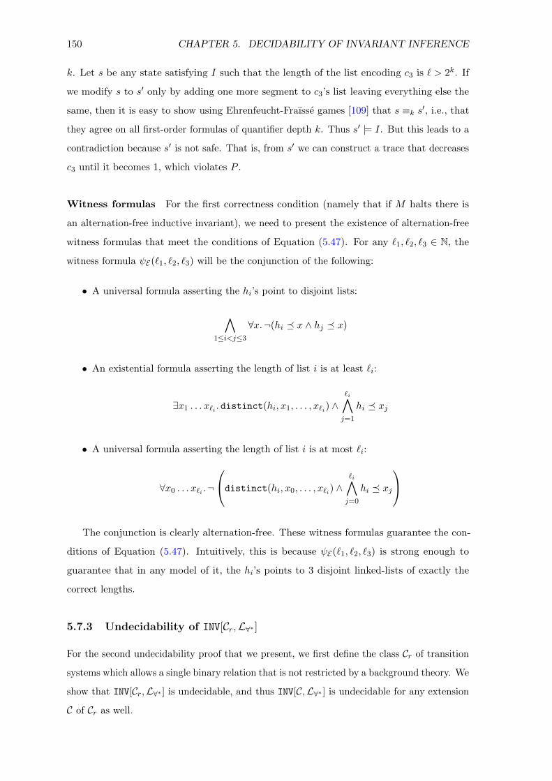
150 CHAPTER 5. DECIDABILITY OF INVARIANT INFERENCE
k. Let s be any state satisfying I such that the length of the list encoding c3 is ` > 2k. If
we modify s to s′ only by adding one more segment to c3’s list leaving everything else the
same, then it is easy to show using Ehrenfeucht-Fraısse games [109] that s ≡k s′, i.e., that
they agree on all first-order formulas of quantifier depth k. Thus s′ |= I. But this leads to a
contradiction because s′ is not safe. That is, from s′ we can construct a trace that decreases
c3 until it becomes 1, which violates P .
Witness formulas For the first correctness condition (namely that if M halts there is
an alternation-free inductive invariant), we need to present the existence of alternation-free
witness formulas that meet the conditions of Equation (5.47). For any `1, `2, `3 ∈ N, the
witness formula ψE(`1, `2, `3) will be the conjunction of the following:
• A universal formula asserting the hi’s point to disjoint lists:
∧1≤i<j≤3
∀x.¬(hi � x ∧ hj � x)
• An existential formula asserting the length of list i is at least `i:
∃x1 . . . x`i . distinct(hi, x1, . . . , x`i) ∧`i∧j=1
hi � xj
• A universal formula asserting the length of list i is at most `i:
∀x0 . . . x`i .¬
distinct(hi, x0, . . . , x`i) ∧`i∧j=0
hi � xj
The conjunction is clearly alternation-free. These witness formulas guarantee the con-
ditions of Equation (5.47). Intuitively, this is because ψE(`1, `2, `3) is strong enough to
guarantee that in any model of it, the hi’s points to 3 disjoint linked-lists of exactly the
correct lengths.
5.7.3 Undecidability of INV[Cr,L∀∗ ]
For the second undecidability proof that we present, we first define the class Cr of transition
systems which allows a single binary relation that is not restricted by a background theory. We
show that INV[Cr,L∀∗ ] is undecidable, and thus INV[C,L∀∗ ] is undecidable for any extension
C of Cr as well.

5.7. UNDECIDABILITY AND COMPLEXITY OF INV[C,L] 151
Definition 5.50 (Cr). We denote by Cr the class of EPR transition systems where Σ
contains a single binary relation symbol r, any finite number of nullary relation symbols,
and 4 constant symbols, and there is no background theory (i.e., Γ = ∅).
Therefore, the state space of T ∈ Cr is STRUCT[Σ] (no background theory). This
subsection proves the following:
Theorem 5.51. INV[C,L∀∗ ] is undecidable for every class C that extends Cr.
To show undecidability of INV[Cr,L∀∗ ], we present an encoding Er, which uses the single
unrestricted binary relation r allowed by Cr to encode the counters. For the correctness
of the reduction we must show universal witness formulas ψE (as per L∀∗) that meet the
conditions of Equation (5.47).
We use the same idea of Section 5.7.2, namely to encode the counters c1, c2, c3 using 3
disjoint linked-lists whose heads are h1, h2, h3, and to use the list lengths to encode counter
values. However, this time we will use the relation r to directly capture next pointer edges.
We first explain why the fact that L∀∗ allows only universal invariants (as opposed to
alternation-free) makes the reduction trickier, and then present the encoding that can be
used for this reduction.
Encoding A zero-attempt is to make r be �, and use the transition formulas and witness
formulas to enforce the theory Γ�. This approach is bound to fail, since INV[CDP,L∀∗ ] is
decidable, but it is useful to understand where exactly it fails. The second direction of the
reduction (if M does not halt then there is no inductive invariant) will be correct exactly
as it was in Section 5.7.2, but the first direction will fail: since we are targeting L∀∗ , we
must present universal witness formulas and these do not exist. Intuitively, this is because
with a universal formula we will only be able to approximate ci = `i as ci ≤ `i, which is not
sufficient for Equation (5.47).
To make the reduction work, we must take advantage of the fact that r is not restricted
by a background theory. We do this by using r to encode list edges directly. It is easy to use
r to express linked-lists operations such as prepending to a linked-list, removing an element
from the head of a list, and checking if the head has an outgoing edge. Thus, we can use r to
write the formulas inci, deci, idi, zeroi, and init to express the same linked-lists operations
as in Section 5.7.2, but this time using r and not �. Figure 5.49(b1) provides an example of
a structure that arises in this encoding for c1 = 3, c2 = 0 and c3 = 2.
However, this also fails. The reason is that any universal formula is closed under
substructure (unlike alternation-free formulas), and a structure that contains a linked-list

152 CHAPTER 5. DECIDABILITY OF INVARIANT INFERENCE
of length > 0, has a substructure where the head of the list does not have an r edge (if we
remove the first node after the head from the domain), and this substructure will satisfy
zeroi. This is demonstrated by Figure 5.49(b2) which is a substructure of Figure 5.49(b1),
but zero3 (wrongfully) holds in it. For this reason, any universal ψE cannot guarantee that
ψE(`1, `2, `3)⇒ ¬zeroi for `i 6= 0.
This can be fixed by adding another constant symbol t, to represent a common tail of
the linked-lists, and changing the formulas as follows:
• inci will prepend a new node to list i (creating a new r edge)
• deci will remove a node from the start of list i, assuming hi 6= t
• idi will keep hi unchanged
• zeroi will test if hi = t
• init will say that r is empty and headi = t for i = 1, 2, 3
The key idea is that since the common tail is guarded by a constant, no “transition to
substructure” can transform a list of length > 0 to a list of length 0. Note however that a
transition to substructure can remove elements that are part of the r-path from hi to t from
the domain, thus making the list disconnected.
Figure 5.49(c1) provides an example of the resulting encoding Er for c1 = 3, c2 = 0 and
c3 = 2. In this case, the substructure in Figure 5.49(c2) no longer satisfies zero3.
Correctness The second correctness condition of the reduction (if M does not halt then
there is no universal inductive invariant) is correct for this encoding by the same arguments
provided for E� (it is not expressible in first-order logic to say that the length of an r-path is
even). For the first correctness condition (if M halts there is a universal inductive invariant),
we present universal witness formulas that meet the conditions of Equation (5.47).
Witness formulas For any `1, `2, `3 ∈ N, define the witness formula ψE(`1, `2, `3) as:
∧i∈{1,2,3}
∀x0 . . . x`i .
`i∧j=0
((hi = x0 ∧
j−1∧k=0
r(xk, xk+1))→ (xj = t↔ j = `i))
These witness formulas are universal, and they satisfy the conditions for inductiveness of
Equation (5.47). Intuitively, the witness formulas make sure that all r-paths of length at
most `i starting from hi are consistent with the fact that list i is of length `i: paths shorter

5.7. UNDECIDABILITY AND COMPLEXITY OF INV[C,L] 153
than `i must not end in t, and paths of length `i must end in t. We note that these witness
formulas admit structures in which the three lists are not disjoint, but this is not problematic
for the reduction.
5.7.4 Complexity of INV[CDP,L∀∗ ] is Non-Elementary
As we saw in Section 5.5, INV[CDP,L∀∗ ] is decidable. In this section, we show that the
complexity of INV[CDP,L∀∗ ] is non-elementary. Therefore this is also true for any (C,L)
extending (CDP,L∀∗), e.g., by the constructions presented in Section 5.6.
Theorem 5.52. The complexity of INV[CDP,L∀∗ ] is non-elementary.
Proof. We prove the theorem by a reduction from the reachability problem of lossy counter
machines, which is known to have non-elementary complexity [211, 212], to the complement
of INV[CDP,L∀∗ ]. The reachability problem for lossy counter machines is: given a counter
machine M = (Q, c1, . . . , ck) and qgoal ∈ Q, is there a trace of M under the lossy semantics
that leads from the initial configuration (q1, 0, . . . , 0), to a configuration with qgoal. Recall
that the lossy semantics lets the value of any counter decrease non-deterministically in any
transition.
The input of the reduction is (M, qgoal), and the output is (T, P, L) ∈ (CDP,L∀∗) such
that:
M has a lossy trace to qgoal ⇔ (T, P, L) 6∈ INV[CDP,L∀∗ ]
According to Section 5.5, (CDP,L∀∗), satisfies the conditions of Theorem 5.6. Therefore,
we can apply Corollary 5.12 and get:
(T, P, L) 6∈ INV[CDP,L∀∗ ] ⇔ T ∀∗ 6|= P
Therefore, it suffices to show that
M has a lossy trace to qgoal ⇔ T ∀∗ 6|= P (5.53)
To construct T = (Σ,Γ, ι, τ) and P that satisfy Equation (5.53), we use the same encoding
E� presented in Section 5.7.2. The only difference is that for this reduction we do not need
the special counter that always holds even values, and we just model the counters of the
input machine M . We encode Q with nullary relations and the values of the k counters using
� and k disjoint linked-lists whose heads are h1, . . . , hk, where the lengths of the lists keep

154 CHAPTER 5. DECIDABILITY OF INVARIANT INFERENCE
the values of the counters. The formulas for the initial state and the transition relation are
constructed as in Sections 5.7.1 and 5.7.2, and the safety property is given by P = ¬qgoal.
To see that the described T and P satisfy Equation (5.53), recall that T ∀∗ 6|= P iff
T has a ∀∗-relaxed trace to a state that violates P , where a ∀∗-relaxed trace can make
transitions to substructures (since v∀∗ is the substructure relation). The punch line is that
for the encoding of Section 5.7.2, these transitions exactly correspond to decrements of the
counters. For a linked-list represented by � and a constant for the head, any substructure is
a linked-list with less elements. (For an example, see Figure 5.49(a1) and its substructure
Figure 5.49(a2).) Therefore, by the construction of T we get that ∀∗-relaxed traces of T
exactly correspond to lossy traces of the counter machine M , and thus Equation (5.53) holds,
which completes the proof.
5.8 Related Work for Chapter 5
Decidability for infinite-state systems via wqo’s Following [5–7, 9], well-quasi-orders
and well-structured (monotonic) transition systems (WSTSs) have become a standard
technique for proving decidability of various problems over infinite-state systems (e.g., [76]).
Often a WSTS is obtained by relaxing the semantics of a transition system to a lossy semantics.
The classical examples of this are lossy channel systems [4], lossy counter machines (e.g., [168])
and vector addition systems or Petri nets (e.g., [150]). In [38, 86], this technique is applied
to array-based transition systems, states are identified with finitely-generated models, and
the quasi-order on states is the substructure relation.
The common approach in these works is to consider a system under lossy semantics
or via an abstraction, and to analyze the decidability of the safety of the lossy/abstract
system. Our work focuses on transition systems formalized using first-order logic, and takes
the viewpoint of restricting potential inductive invariants to some language L, and then
analyzing the decidability of invariant inference in L. The two views are connected: every
particular language L can be regarded as an abstraction, where the abstract domain is
formulas in L; or as a lossy semantics, with lossy transitions according to vL. Indeed, TL
can alternatively be formulated as a monotonic transition system, and this can be viewed as
monotonic abstraction as in [9].
Our use of first-order logic together with a formalism that is parameterized by L, allows
the systematic constructions presented in Section 5.6, which are able to construct restricted
languages and wqo’s that are applicable to complicated systems like the learning switch. From
a practical perspective, using logic enables to use existing decision procedures in the invariant

5.8. RELATED WORK FOR CHAPTER 5 155
inference process. The operation AvoidL corresponds to concepts found both in IC3/PDR
algorithms [34, 116] and in decision procedure based abstract interpreters, e.g., [220], that
automate the process of inferring inductive invariants. Our work can be seen as studying the
conditions required for termination of such procedures, and the conditions under which the
underlying problem is undecidable and thus divergence occurs for infinitely many instances.
nIndeed, in [116], our results have been used to obtain termination guarantees for PDR∀, a
variant of IC3/PDR that finds universally quantified invariants, in cases where v∀∗ is a wqo.
Linked-lists & counter machines In [32], it was observed that linked-list programs
are counter machines. While the safety of counter machines is undecidable, the safety of
lossy counter machines is decidable with non-elementary complexity [211]. In the case of
linked-lists, our work can be seen as combining these two interesting results: “Linked-lists
with alternation-free invariants are counter machines” (and therefore undecidable), and
“Linked-lists with universal invariants are lossy counter machines” (and therefore decidable
with non-elementary complexity).
In [10, 11], monotonic abstractions are defined for linked data structures. The wqo on
heaps defined there is semantically similar to v∀∗ with �, but it is defined via tree operations
and not via logic. This makes the result of Section 5.5 more powerful because it also provides
unlimited unary predicates, as well as being amenable to the constructions of Section 5.6.
The wqo of [10] results in a slightly less precise abstraction compared to that of Section 5.5,
as it also allows edge deletion (which is not allowed in v∀∗ with �). Interestingly, the proof
in [10] does not use Kruskal’s Tree Theorem, which is the basis for our result.
Undecidability There are many undecidability results for safety of infinite state systems,
e.g., [32, 39]. For the related problem INV of inferring inductive invariants we show two
interesting undecidability results: for universal invariants over arbitrary domains; and for
alternation-free formulas over the theory of linked-list reachability.
Completeness of abstract interpretation The theoretical study of the precision of
abstract interpretation is an ongoing research area. Usually completeness for abstract
interpretation means that the abstract domain is precise enough to prove all interesting
safety properties, e.g., [87]. In our terms, this means that INV = SAFE, i.e., that all
safe programs have an inductive invariant expressible in the abstract domain. Since we
are interested in automatically analyzing Turing-complete programs (for which SAFE is
undecidable), we consider the completeness problem at a later binding time. Essentially, INV

156 CHAPTER 5. DECIDABILITY OF INVARIANT INFERENCE
asks if the abstract domain is precise enough for a given property in a given program.
A very interesting twist on completeness of abstract interpreters is considered in [88] which
algorithmically studies the completeness of certain abstract domains for certain questions.
Numeric domains For numeric domains (e.g., intervals), techniques such as widening and
policy iteration (e.g. [83]) are used to prove the correctness of many infinite state systems.
Surprising results in [82, 217] show that for some numeric domains and programs, precise
information can be computed, thus solving INV. However, it is not known how to extend
these techniques and results beyond numeric template domains, for example to the context
of first-order logic considered here.

Chapter 6
Interactive Inference of Universal
Invariants
This chapter is based on the results published in [186].
As we have seen in Chapters 3 and 4, first-order logic and specifically EPR can capture
interesting and challenging verification problems. That is, one can encode both the system
and its inductive invariant in such a way that verification conditions are in EPR, and then
use automated solvers to reliably check the verification conditions, and if the invariant is not
inductive, a finite counterexample to induction is provided. One problem that still remains
is finding the inductive invariants themselves. In Chapter 5, we have explored this problem
from a theoretical perspective and obtained some decidability and undecidability results.
In this chapter, we adopt a more practical mindset and attempt to answer the following
question: how can we help the user find inductive invariants, beyond providing counterexam-
ples in the classical guess and check process? We focus on universally quantified inductive
invariants, and use the connection introduced in Chapter 5 between universal invariants,
substructures, and diagrams. We also exploit the finite model property of EPR. Using these
concepts, we develop a graphical interaction mode that allows the user to guide generalization
from counterexamples to induction in an interactive process for finding universally quantified
inductive invariants. The developed methodology is implemented as part of the Ivy deductive
verification system, and we also present an empirical evaluation for several examples that
have universal inductive invariants.
157
158 CHAPTER 6. INTERACTIVE INFERENCE OF UNIVERSAL INVARIANTS
6.1 Overview & Illustration
This section provides an informal overview of the interactive verification methodology we
develop, aimed at finding universally quantified inductive invariants. This methodology is
implemented as part of the Ivy deductive verification system.
Design philosophy The methodology we develop is inspired by proof assistants such
as Isabelle/HOL [181] and Coq [26] which engage the user in the verification process. We
also aim to exploit the success of tools such as Z3 [61] which can be very useful for bug
finding, verification, and static analysis, and on automated invariant inference techniques
such as [116]. We aim to balance between the predictability and visibility of proof assistants,
and the automation of decision procedures and automated invariant inference techniques.
Compared to fully automated techniques, we adopt a different philosophy which permits
visible failures at the cost of more manual work from the users. Compared to proof assistants,
we aim to provide the user with automated assistance, solving well-defined decidable problems.
To obtain this, we restrict ourselves to systems that can be expressed as EPR transition
systems, and focus on finding universally quantified inductive invariants. These restrictions
guarantee that the tasks performed automatically are actually solving decidable problems.
Running example: leader election in a ring protocol We illustrate the interactive
methodology on the example presented in Section 3.1.1, for a distributed leader election
protocol in a ring topology. Figure 3.1 depicts the RML model of this protocol. The ring
topology is modeled using the btw path relation, as explained in Section 3.3.3. Recall that
we wish to verify the safety property that the protocol never elects more than one leader. As
presented in Section 3.1.1, safety of this protocol can be proven with a universal inductive
invariant, given by Equations (3.3) to (3.5). We now ask ourselves how we might discover
such an inductive invariant without knowing it. We use this example to illustrate our
methodology for finding inductive invariants by an interactive process between the user and
well-defined, decidable, automated queries.
Graphical visualization of states A key ingredient in the interactive process is a
graphical representation. Ivy displays states of the protocol as graphs, where the vertices
represent elements, and edges represent relations and functions. As an example, consider
the state of the leader election protocol depicted in Figure 6.1. This state has two nodes
and two IDs, represented by vertices of different shapes. Unary relations are displayed using
vertex labels. For example, in Figure 6.1, node 1 is labeled leader , and node 2 is labeled

6.1. OVERVIEW & ILLUSTRATION 159
Figure 6.1: Graphical representation of a protocol state for the leader election in a ringprotocol.
Figure 6.2: Flowchart of bounded verification.
¬leader , denoting that the leader relation contains only node 1. Binary relations such as ≤and msg are displayed using directed edges. Higher-arity relations are displayed by means
of their projections or derived relations. For example, the ternary relation btw is displayed
by the derived binary relation link which captures a single ring edge, and is defined by
link(x, y) ≡ ϕs(x, y) (as in Section 3.3.3, Figure 3.18). Functions such as id are displayed
similarly to relations. The state depicted in Figure 6.1 contains two nodes, node 1 and node
2, such that the ID of node 1 is lower (by ≤) than the ID of node 2. A message with the
ID of node 2 is pending at node 2, as indicated by the msg edge. This state is clearly not
reachable in the protocol. However, as we shall see later, we encounter this state as part of a
counterexample to induction, during the interactive search for the inductive invariant.
Bounded verification While our end goal is to verify the system for an unbounded
number of execution steps (via a universally quantified inductive invariant), we also present
a step of symbolic model debugging via bounded verification, i.e., unrolling the transition
relation a bounded number of times. This step is extremely useful in practice, since one
rarely writes a correct model on the first attempt, with errors ranging from minor typos
to more serious issues. As we shall see, bounded unrolling will also be exploited for the

160 CHAPTER 6. INTERACTIVE INFERENCE OF UNIVERSAL INVARIANTS
interactive search for an inductive invariant.
For example, suppose our initial modeling of the leader election protocol missed the axiom
stating leaders have unique IDs (Figure 3.1 line 12). We can discover this by performing
bounded verification with a bound of 4 transitions. This results in the error trace depicted
in Figure 6.3. In this trace, node 1 identifies itself as a leader when it receives the message
with the ID of node 2 since they have the same ID (id 1), and similarly for node 2, leading to
violation of the assertion. After adding the missing axiom, we can run Ivy with an unrolling
bound of 10 transitions to debug the model, and we do not get a counterexample trace.
While many tools offer debugging of formal models by bounded verification (e.g., Al-
loy [114], TLA+ [137]), we note that the bounded verification we perform here also exploits
the restriction to EPR transition systems and EPR’s finite model property. Unlike other
verification systems, Ivy does not require an a priori bound on the size of the states considered
(e.g., number of nodes). Instead, Ivy only requires a bound on the number of transitions to
unroll. Of course, due to the properties of EPR, this also implies a bound on the size of the
possible models, but this bound is implicit, and the user need not provide it.
In our experience, most protocols can be verified for about 10 transitions in a few minutes,
which is extremely useful for eliminating typos and minor issues with the modeling of the
protocol and/or formulation of the safety property. Once bounded verification does not find
more bugs, the user can prove unbounded correctness by searching for an inductive invariant,
as explained next.
Interactive search for universally quantified inductive invariants The second
phase of the verification is to find a universally quantified inductive invariant that proves
that the system is correct for any number of transitions. This phase requires more user effort
but enables ultimate safety verification. Recall that an invariant I is inductive if: (i) all
initial states satisfy I (initiation); (ii) every state satisfying I also satisfies the desired safety
properties (safety); and (iii) I is closed under transitions of the system, i.e., a transition from
any arbitrary state satisfying I results in a new state that also satisfies I (consecution).
If the user has a universally quantified inductive invariant in mind, Ivy can automatically
check if it is indeed an inductive invariant. Due to the restrictions of EPR, this check is
guaranteed to terminate with either a proof showing that the invariant is inductive or a
finite counterexample to induction (CTI), which can be depicted graphically and presented
to the user, as explained before. A CTI does not necessarily imply that the safety property
is violated — only that I is not an inductive invariant. Coming up with inductive invariants
for infinite-state systems is very difficult. Therefore, Ivy supports an interactive procedure

6.1. OVERVIEW & ILLUSTRATION 161
(a)
(b)
(c)
(d)
(e)
Figure 6.3: An error trace found by BMC for the leader protocol, when omitting the factthat node IDs are unique. (a) an initial state; (b) node 1 sent a message to node 2; (c) node2 sent a message to node 1; (d) node 1 processed a pending message and became leader; (e)node 2 processed a pending message and became leader, there are now two leaders and thesafety property is violated.

162 CHAPTER 6. INTERACTIVE INFERENCE OF UNIVERSAL INVARIANTS
Figure 6.4: Flowchart of the interactive search for an inductive invariant.
for gradually obtaining an inductive invariant or deciding that the model or safety property
need to be revised.
The search for an inductive invariant starts with a (possibly empty) set of universally
quantified conjectures, whose conjunction is the current candidate inductive invariant. The
search advances based on CTIs according to the procedure described in Figure 6.4. When a
CTI is found it is displayed graphically, and the user has 3 options:
1. The user understands that there is a bug in the model or safety property, in which
case they revise the RML program and start over in Figure 6.2. Note that in this
case, the user may choose to retain some conjectures reflecting gained knowledge of
the expected protocol behavior.
2. The user understands that one of the conjectures is wrong, in which case they remove
it from the conjecture set, weakening the candidate invariant.
3. The user judges that the CTI is not reachable. This means that the invariant needs to
be strengthened by adding a new conjecture. The new conjecture should eliminate the
CTI, and should generalize from it. This is the most creative task, and our approach
for it is explained below.
Graphical visualization of conjectures To allow the user to examine and modify pos-
sible conjectures, Ivy provides a graphical visualization of universally quantified conjectures.
Such a conjecture asserts that some sub-configuration (i.e., logical substructure) of the
system is not present in any reachable state. That is, any state of the system that contains
this sub-configuration is not reachable. Ivy graphically depicts such conjectures by displaying

6.1. OVERVIEW & ILLUSTRATION 163
the forbidden sub-configuration. Sub-configurations are visualized similarly to the way states
are displayed, but with a different semantics.
As an example consider the conjecture depicted in Figure 6.6 (b). The visualization
shows two nodes and their distinct IDs; node 1 is shown to be a leader, while node 2 is
not a leader. Furthermore, the ID of node 1 is lower (by ≤) than the ID of node 2. Note
that no pending messages appear (no msg edges), and there is also no information about
the topology (no link or btw edges). Viewed as a conjecture, this graph asserts that in any
reachable state, there cannot be two nodes such that the node with the lower ID is a leader
and the node with the higher ID is not a leader. Thus, this conjecture excludes infinitely
many states with any number of nodes above 2 and any number of pending messages. It
excludes all states that contain any two nodes such that the node with the lower ID is a
leader and the node with the higher ID is not a leader.
Figure 6.6 (c) depicts an even stronger (more general) conjecture: unlike Figure 6.6 (b),
node 2 is not labeled with ¬leader nor with leader . This means that the conjecture in
Figure 6.6 (c) excludes all the states that contain two nodes such that the node with the
lower ID is a leader, regardless of whether the other node is a leader or not.
Obtaining helpful CTIs Since we rely on the user to guide the generalization from CTIs,
it is critical to display a CTI that is both easy to understand, and indicative of the proof
failure. Therefore, Ivy searches for “minimal” CTIs. The procedure Find Minimal CTI used
in Figure 6.4 (and explained in Section 6.2.3) automatically obtains a minimal CTI based on
user provided minimization criteria. Examples include minimizing the number of elements,
and minimizing certain relations (e.g., minimizing the msg relation to have few pending
messages). This is performed automatically and reliably by reducing the minimization
problem to a series of EPR queries.
Interactive generalization from CTIs When a CTI represents an unreachable state,
we should strengthen the invariant by adding a new conjecture to eliminate the CTI. One
possible universally quantified conjecture is the one which excludes all states that contain the
concrete CTI as a sub-configuration (i.e., the diagram of the CTI, as presented in Chapter 5).
However, this conjecture may be too specific, as the CTI contains many features that are
not relevant to the failure. This is where generalization is required, or otherwise we may end
up in a diverging refinement loop, always strengthening the invariant with more conjectures
that are all too specific. (Even if v∀∗ is a wqo, a naive iteration may take prohibitively long
before its assured termination.)

164 CHAPTER 6. INTERACTIVE INFERENCE OF UNIVERSAL INVARIANTS
C0 ∀n1, n2.¬(leader(n1) ∧ leader(n2) ∧ n1 6= n2
)C1 ∀n1, n2.¬
(n1 6= n2 ∧ leader(n1) ∧ id(n1) ≤ id(n2)
)C2 ∀n1, n2.¬
(n1 6= n2 ∧msg(id(n1), n1) ∧ id(n1) ≤ id(n2)
)C3 ∀n1, n2, n3.¬
(btw(n1, n2, n3) ∧msg(id(n2), n1) ∧ id(n2) ≤ id(n3)
)Figure 6.5: The conjectures found using Ivy for the leader election protocol. C0 is thesafety property, and the remaining conjectures (C1 - C3) were produced interactively. Theconjunction C0 ∧ C1 ∧ C2 ∧ C3 is an inductive invariant for the protocol.
It is at this crucial point that we attempt to utilize the user’s intuition, and not rely
on automation. Ivy asks the user to guide generalization from CTIs. To achieve this, Ivy
presents the user with a concrete CTI, and lets the user eliminate some of the features of
the CTI that the user judges to be irrelevant (e.g., by marking some relations as irrelevant).
This already defines a generalization of the CTI that excludes more states.
Next, the BMC + Auto Generalize procedure applies bounded verification (with a user
specified bound) to check the user’s suggestion, and also to generalize further. If the test
fails, it means that the user’s generalized conjecture is violated in a reachable state, and a
concrete counterexample trace is displayed to let the user diagnose the problem. If the test
succeeds (i.e., the bounded verification formula is unsatisfiable), Ivy automatically suggests
a stronger generalization, based on a minimal unsatisfiable core. The user then decides
whether to accept the suggested conjecture and add it to the invariant, or to change the
parameters in order to obtain a different suggestion.
Next, we walk through this process for the leader election protocol, demonstrating the
different stages, until we obtain an inductive invariant that proves the protocol’s safety.
Illustration using the leader election protocol Figure 6.5 summarizes the 3 iterations
Ivy required to find an inductive invariant for the leader election protocol. The initial set of
conjectures contains only C0, which is simply the specified safety property that there cannot
be two distinct leaders elected.
In the first iteration, since C0 alone is not inductive, Ivy applies Find Minimal CTI.
This results in the CTI depicted in Figure 6.6 (a1). Figure 6.6 (a2) depicts a successor
state of (a1) reached after node 2 receives the pending message with its ID. The state (a1)
satisfies C0, whereas (a2) violates it, making (a1) a CTI. After examining this CTI, the user
judges that the state (a1) is unreachable, with the intuitive explanation that node 1 identifies
itself as a leader despite the fact that node 2 has a higher ID. Thus, the user generalizes
away the irrelevant information, which includes msg and the ring topology, resulting in the

6.1. OVERVIEW & ILLUSTRATION 165
(a1) (a2)
(b)
(c)
Figure 6.6: The 1st CTI generalization step for the leader protocol, leading to C1. (a1) TheCTI state that has one leader, but makes a transition to a state (a2) with two leaders. Theroot cause is that a node with non-maximal ID is a leader. (b) A generalization created by theuser by removing the topology information and the msg relation (c) Further generalizationobtained by BMC + Auto Generalize, which removed the fact that node 2 is not a leader.

166 CHAPTER 6. INTERACTIVE INFERENCE OF UNIVERSAL INVARIANTS
(a1) (a2)
(b)
Figure 6.7: The 2nd CTI generalization step for the leader protocol, leading to C2. (a1)The CTI state and its successor (a2) violating C1. The root cause is that a node withnon-maximal ID has a pending message with its own ID. (b) A generalization created by theuser by removing the topology information and the leader relation. This generalization wasvalidated but not further generalized by BMC + Auto Generalize.
generalization depicted in Figure 6.6 (b).
Next, the user applies BMC + Auto Generalize with bound 3 to this generalization. The
test succeeds, and Ivy suggests the generalization in Figure 6.6 (c), where the information that
node 2 is not a leader is also abstracted away. The user approves this generalization, which
corresponds to conjecture C1 shown in Figure 6.5, so C1 is added to the set of conjectures.
If the user had used bound 2 instead of 3 when applying BMC + Auto Generalize, then
Ivy would have suggested a stronger generalization that also abstracts the ID information,
and states that if there are two distinct nodes, none of them can be a leader. This conjecture
is bogus, but it is true for up to 2 transitions from the initial state (since with 2 nodes,
a node can only become a leader after a send action followed by 2 receive actions). It is
therefore the role of the user to select and adjust the bound for automatic generalization,
and to identify bogus generalizations when they are encountered.
After adding the correct conjecture C1, Ivy displays the CTI depicted in Figure 6.7 (a1)
with its successor state (a2). Note that (a2) does not violate the safety property, but it violates
C1 that was added to the invariant, since a node with a non-maximal ID becomes a leader.
The user examines (a1) and concludes that it is not reachable, since it has a pending message

6.1. OVERVIEW & ILLUSTRATION 167
(a1) (a2)
(b)
(c)
Figure 6.8: The 3rd CTI generalization step for the leader protocol, leading to C3. (a1) TheCTI state and its successor (a2) which violates C2. The root cause is that node 1 has apending message with the ID of node 2, even though node 3 is on the path from node 2 tonode 1 and has an ID higher than node 2’s ID (equivalently, node 2 is between node 1 andnode 3 and has a lower ID than node 3’s ID). (b) A generalization created by the user byremoving the leader relation. The generalization does not contain link , only btw . (c) Furthergeneralization obtained by BMC + Auto Generalize, which eliminated id1.

168 CHAPTER 6. INTERACTIVE INFERENCE OF UNIVERSAL INVARIANTS
to node 1 with its own ID, despite the fact that node 2 has a higher ID. Here, the user again
realizes that the ring topology is irrelevant and abstracts it away. The user also abstracts
away the leader information. On the other hand, the user keeps the msg information, in
accordance with the intuitive explanation of why the CTI is not reachable. The resulting
user-defined generalization is depicted in Figure 6.7 (b). BMC + Auto Generalize with
bound 3 validates this generalization for 3 transitions, but does not manage to generalize
any further. Thus, the generalization is converted to C2 in Figure 6.5 which is added to the
invariant, and the process continues.
Finally, Figure 6.8 (a1) and (a2) depicts a CTI that leads to a violation of C2. This CTI
contains three nodes, with a pending message that appears to bypass a node with a higher
ID. This time, the user does not abstract away the topology since it is critical to the reason
the CTI is not reachable. The user only abstracts the leader information, which leads to
the generalization depicted in Figure 6.8 (b). Note that in the generalized conjecture we no
longer consider the link relation, but rather the btw relation. This expresses the fact that,
as opposed to the concrete CTI, the conjecture generalizes from the specific topology of a
ring with exactly 3 nodes, to a ring that contains it as a sub-configuration, i.e., a ring with
at least 3 nodes that are not necessarily immediate neighbors of each other. We do require
that the three nodes are ordered in such a way that node 2 is between node 1 and node 2 in
the ring (equivalently, node 3 is between node 2 and node 1).
Applying BMC + Auto Generalize with a bound of 3 to Figure 6.8 (b) confirms this
conjecture, and automatically abstracts away the ID of node 1, which results in the conjecture
depicted in Figure 6.8 (c), which corresponds to C3 in Figure 6.5. The user adds this conjecture
to the invariant. After adding C3, Ivy reports that I = C0 ∧ C1 ∧ C2 ∧ C3 is an inductive
invariant for the leader election protocol.
6.2 Interactive Methodology for Safety Verification
In this section, we elaborate and formalize the ideas outlined in Section 6.1. Recall that we
are interested in safety verification on an RML program. The RML program is compiled
to a transition system T = (Σ,Γ, ι, τ) and a safety property P (see Section 2.5), and we
assume they form an EPR transition system. We allow stratified functions, but require that
the conjunction of Γ, ι, τ , and ¬P , is in the many sorted EPR fragment (i.e., the functions
and quantifier alternations are stratified).
The key idea is to combine automated analysis with user guidance in order to construct
a universally quantified inductive invariant that proves safety. The next subsection describes

6.2. INTERACTIVE METHODOLOGY FOR SAFETY VERIFICATION 169
a preliminary stage for debugging the RML program, and the following subsections describe
our interactive methodology of constructing universal inductive invariants.
6.2.1 Debugging via Symbolic Bounded Verification
Before starting the search for an inductive invariant, it makes sense to first search for bugs
in the RML program. This can be done by unrolling the transition relation τ a bounded
number of times. We define an assertion ϕ to be k-invariant if it holds in all states reachable
after at most k transitions from an initial state. Thus, ϕ is k-invariant if and only if the
following formula is unsatisfiable for any j ≤ k:
(j∧i=0
∧Γ(Σi)
)∧ ι(Σ0) ∧
(j−1∧i=0
τ(Σi,Σi+1)
)∧ ¬ϕ(Σj) (6.9)
where Σi = {ai | a ∈ Σ}, and τ(Σi,Σi+1) denotes the formula over vocabulary Σi ] Σi+1
obtained from τ when every symbol a ∈ Σ is replaced by ai and every symbol a′ ∈ Σ′ is
replaced by ai+1. The formulas∧
Γ(Σi), ι(Σ0), and ϕ(Σj), are defined similarly.
Since we assume T to be an EPR transition system, checking k-invariance of any ∀∗∃∗-formula ϕ is decidable. Furthermore, if such a ϕ is not k-invariant, we can obtain a finite
model of Equation (6.9) for some j ≤ k. This model represents an execution trace that
executes j loop iterations and reaches a state that violates ϕ. This trace can be graphically
displayed to the user as a concrete counterexample to the invariance of ϕ. Note that while
checking k-invariance bounds the number of loop iterations, it does not bound the size of
the states. Thus, if a property is found to be k-invariant, it holds in all states reachable
by k iterations. This is in contrast to finite-state bounded model checking techniques that
bound the state space.
The first step when using Ivy is to model the system at hand as an RML program, and
then debug the program by checking k-invariance of the safety property P , as illustrated
in Figure 6.2. If a counterexample is found, the user can examine the trace and modify
the RML program to either fix a bug in the code, or to fix a bug in the specification (the
assertions that determine P ). Once no more counterexample traces exist up to a bound that
satisfies the user, the user moves to the second step of constructing a universal inductive
invariant that proves the safety of the system for unbounded number of iterations.

170 CHAPTER 6. INTERACTIVE INFERENCE OF UNIVERSAL INVARIANTS
6.2.2 Interactive Search for Universal Inductive Invariants
Ivy assists the user in obtaining a universal inductive invariant. Recall that a formula I is
an inductive invariant for a transition system T = (Σ,Γ, ι, τ) if the verification conditions
defined in Section 2.4.2 are unsatisfiable. Moreover, if I is a universally quantified formula,
then the verification conditions are in EPR, so checking them is decidable, and if I is not an
inductive invariant then we can obtain a finite state s that is a counterexample to one of the
conditions. Such a state s is a counterexample to induction (CTI).
Our methodology interactively constructs a universal inductive invariant represented
as a conjunction of conjectures, i.e., I =∧ni=1 ϕi. Each conjecture ϕi is a closed universal
formula. In the sequel, we interchangeably refer to I as a set of conjectures and as the
formula obtained from their conjunction.
Our methodology, presented in Figure 6.4, guides the user through an iterative search for
a universal inductive invariant I by generalization from CTIs. We maintain the fact that all
conjectures satisfy initiation Γ, ι |= ϕi, so each CTI we obtain is always a state that satisfies
all conjectures, but either violates the safety property P , or can lead to a state that violates
one of the conjectures by executing a τ transition.
Initialization The search starts from a given set of conjectures as a candidate inductive
invariant I. For example, I can be initialized to true. If P is universal, then I can initially
include P (after checking that P is 0-invariant, i.e., satisfied by initial states). If the search
starts after a modification of the RML program (e.g., to fix a bug or add a new feature
to the model), then conjectures that were learned before can be reused. Additional initial
conjectures can be computed by applying basic abstract interpretation techniques (e.g., using
some predicate abstraction).
Iterations Each iteration starts by (automatically) checking whether the current candidate
I is an inductive invariant. If I is not yet an inductive invariant, a CTI is presented to the
user, which is a state s that either violates P (safety violation), or leads to a state that
violates I via a τ transition (consecution violation). The user can choose to strengthen I by
conjoining it with an additional conjecture that excludes the CTI from I. To this end, we
provide automatic mechanisms to assist in generalizing from the CTI to obtain a conjecture
that excludes it. In case of a consecution violation, the user may also choose to weaken I by
eliminating one (or more) of the conjectures. The user can also choose to modify the RML
program in case the CTI indicates a bug. This process continues until an inductive invariant
is found.

6.2. INTERACTIVE METHODOLOGY FOR SAFETY VERIFICATION 171
For I to be an inductive invariant, all the conjectures ϕi need to be invariants (i.e., hold
in all states reachable at the loop head). This might not hold in the intermediate steps of
the search, but it guides strengthening and weakening: strengthening aims at only adding
conjectures that are invariants, and weakening aims at identifying and removing conjectures
that are not invariants. While strengthening and weakening are ultimately performed by the
user, we provide several automatic mechanisms to assist the user in this process.
Obtaining a minimal CTI When I is not inductive, it is desirable to present the user
with a CTI that is easy to understand, and not cluttered with many unnecessary features.
This also tends to lead to better generalizations from the CTI. To this end, we automatically
search for a “minimal” CTI, where the minimization parameters are defined by the user.
Section 6.2.3 explains this in detail.
Interactive generalization To eliminate the CTI s, the user needs to either strengthen
I to exclude s from I, or, in case of a consecution violation, to weaken I to include a state
reachable from s via τ . Intuitively, if s is not reachable, then I should be strengthened
to exclude it. If s is reachable, then I should be weakened. Clearly, checking whether s
is reachable is infeasible. Instead, we provide the user with a generalization assistance for
coming up with a new conjecture to strengthen I. The goal is to come up with a conjecture
that is satisfied by all the reachable states. During the attempt to compute a generalization,
the user might also realize that an existing conjecture is in fact not an invariant (i.e., it is
not satisfied by all reachable states), and hence weakening is in order. In addition, the user
might also find a modeling bug which means the RML program should be fixed.
Generalizations are explained and formalized in Section 6.2.4, and the interactive general-
ization process is explained in Section 6.2.5. Here again, the user defines various parameters
for generalization, and Ivy automatically finds a candidate that meets the criteria. The user
can further change the suggested generalization and can use additional automated checks to
decide whether to keep it.
Note that if all the conjectures added by the user exclude only unreachable states (i.e., all
are invariants), then weakening is rarely needed. As such, most of the automated assistance
we provide focuses on helping the user obtaining “good” conjectures for strengthening, i.e.,
conjectures that do not exclude reachable states. Weakening will typically be used when
some conjecture turns out to be “wrong” in the sense that it does exclude reachable states.

172 CHAPTER 6. INTERACTIVE INFERENCE OF UNIVERSAL INVARIANTS
6.2.3 Obtaining Minimal CTIs
We refine the search for CTIs by trying to find a minimal CTI according to user adjustable
measures. As a general rule, smaller CTIs are desirable since they are both easier to
understand, which is important for interactive generalization, and more likely to result in
more general (stronger) conjectures. The basic notion of a small CTI refers to the number
of elements in its domain. However, other quantitative measures are of interest as well. For
example, it is helpful to minimize the number of elements (or tuples) in a relation, e.g., if
the relation appears as a guard for protocol actions (such as the msg relation in the leader
election protocol of Figure 3.1). Thus, we define a set of useful minimization measures, and
let the user select which ones to minimize, and in which order.
Minimization measures We consider the following measures for s = (D, I):
• Size of sort s: |D(s)|.
• Number of positive tuples of relation r: |I(r)|.
• Number of negative tuples of relation r: |{e | e 6∈ I(r)}|.
Each measure m induces an order ≤m on structures, and each tuple (m1, . . . ,mt) of
measures induces a “smaller than” relation on structures which is defined by the lexicographic
order constructed from the orders ≤mi .
Minimization procedure Given the tuple of measures to minimize, provided by the user,
Algorithm 6.1 automatically finds a CTI that is minimal with respect to this lexicographic
order. The idea is to conjoin ψcti (which encodes violation of inductiveness) with a formula
ψmin that is computed incrementally and enforces minimality. For a measure m, ϕm(n) is
an ∃∗∀∗ clause stating that the value of measure m is no more than the number n. Such
constraints are added to ψmin for every m, by their order in the tuple, where n is chosen to
be the minimal number for which the constraint is satisfiable (with the previous constraints).
Finally, a CTI that obeys all the additional constraints is computed and returned.
For example, consider a k-ary relation r. We encode the property that the number of
positive tuples of r is at most n as follows: ∃x1, . . . xn.∀y.(r(y) → ∨n
i=1 y = xi), where
x1, . . . , xn, y denote k-tuples of logical variables.

6.2. INTERACTIVE METHODOLOGY FOR SAFETY VERIFICATION 173
Algorithm 6.1: Obtaining a Minimal CTI
1 if ψcti is unsatisfiable then return None;2 ψmin := true ;3 for m in (m1, . . . ,mt) do4 for n in 0, 1, 2, . . . do5 if ψcti ∧ ψmin ∧ ϕm(n) is satisfiable then6 ψmin := ψmin ∧ ϕm(n) ;7 break
8 return s such that s |= ψcti ∧ ψmin
6.2.4 Formalizing Generalizations as Partial Structures
In this subsection we present the notion of a generalization and the notion of a conjec-
ture associated with a generalization. These notions are key ingredients in the interactive
generalization step described in the next subsection.
Recall that a CTI is a structure s = (D, I). Here it is useful for us to treat the
interpretation of a relation symbol r : s1, . . . , sk as a function I(r) : D(s1)× . . .×D(sk)→{0, 1}, and the interpretation of a function symbol f : s1, . . . , sk → s as a function I(f) :
D(s1)× . . .×D(sk)×D(s)→ {0, 1} such that for any x1, . . . , xk ∈ D, I(f)(x1, . . . , xk, y) = 1
for exactly one element y ∈ D. Essentially, we treat functions of arity k as “special” relations
of arity k + 1 that relate each k-tuple to exactly one element. While this differs from the
official definitions of Section 2.1, the difference is unessential, yet it makes the presentation
of generalizations simpler and more uniform.
Generalizations of a CTI are given by partial structures, where relation symbols and
function symbols are interpreted as partial functions. Formally:
Definition 6.10 (Partial Structures). Given a vocabulary Σ and a domain D, a partial
interpretation I of Σ over D associates every k-ary relation symbol r ∈ Σ with a partial
function I(r) : Dk ⇀ {0, 1}, and every k-ary function symbol f ∈ Σ with a partial
function I(f) : Dk+1 ⇀ {0, 1}, such that the sort restrictions are satisfied and also for any
x1, . . . , xk ∈ D, I(f)(x1, . . . , xk, y) = 1 for at most one element y ∈ D. A partial structure
over Σ is a pair (D, I), where I is a partial interpretation of Σ over domain D.
Note that a structure is a special case of a partial structure. Intuitively, generalization
takes place when a CTI is believed to be unreachable, and a partial structure generalizes
a CTI (structure) by turning some values (“facts”) to be undefined or unspecified. For
example, in a partial structure, I(r)(e) might remain undefined for some tuple e. This is
useful if the user believes that the structure is still unreachable, regardless of the value of
I(r)(e). In Figures 6.6 to 6.8, (a1) and (a2) always represent total structures, while (b) and

174 CHAPTER 6. INTERACTIVE INFERENCE OF UNIVERSAL INVARIANTS
(c) represent partial structures.
A natural generalization partial order can be defined over partial structures:
Definition 6.11 (Generalization Partial Order). Let I1 and I2 be two partial interpretations
of Σ over D1 and D2 respectively, such that D2 ⊆ D1. We say that I2 v I1 if for every
relation or function symbol a ∈ Σ, If e ∈ dom(I2(a)), then e ∈ dom(I1(a)) as well, and
I2(a)(e) = I1(a)(e). For partial structures s1 = (D1, I1) and s2 = (D2, s2) of Σ, we say that
s2 v s1 if D2 ⊆ D1 and I2 v I1.
The generalization partial order extends the substructure relation of (total) structures.
Intuitively, s2 v s1 if the interpretation provided by s1 is at least as “complete” (defined) as
the interpretation provided by s2, and the two agree on elements (or tuples) for which s2
is defined. Thus, s2 v s1 when s2 represents more states than s1, and we say that s2 is a
generalization of s1.
From partial structures to conjectures Intuitively, every partial structure s represents
an infinite set of structures that are more specific than s (they interpret more facts and
contain more elements), and the conjecture that a partial structure induces excludes all these
structures (states). Formally, a partial structure induces a universally quantified conjecture
that is obtained as the negation of the diagram of the partial structure, where we extend
classic definition of a diagram (given in Chapter 5, Definition 5.16) from structures to partial
structures.
Definition 6.12 (Diagram for Partial Structures). Let s = (D, I) be a finite partial structure
of Σ and let D′ = {e1, . . . , e|D′|} ⊆ D denote the set of elements ei for which there exists (at
least one) relation or function symbol a ∈ Σ such that ei appears in some tuple of dom(I(a)).
The diagram of s, denoted by Diag(s), is the following formula over Σ:
∃x1 . . . x|D′|. distinct(x1, . . . , x|D′|) ∧ ψ
where ψ is the conjunction of:
• r(xi1 , . . . , xik) for every k-ary relation r in Σ and every i1, . . . , ik s.t.
I(r)(ei1 , . . . , eik) = 1;
• ¬r(xi1 , . . . , xik) for every k-ary relation r in Σ and every i1, . . . , ik s.t.
I(r)(ei1 , . . . , eik) = 0;

6.2. INTERACTIVE METHODOLOGY FOR SAFETY VERIFICATION 175
• f(xi1 , . . . , xik) = xj for every k-ary function f in Σ and every i1, . . . , ik and j s.t.
I(f)(ei1 , . . . , eik , ej) = 1; and
• f(xi1 , . . . , xik) 6= xj for every k-ary function f in Σ and every i1, . . . , ik and j s.t.
I(f)(ei1 , . . . , eik , ej) = 0.
Intuitively, Diag(s) is obtained by treating individuals in D as existentially quantified
variables and explicitly encoding all the facts that are defined in s. Note that we treat
constants as functions of 0 arity, and that for structures s that are not partial, Diag(s) of
Definition 6.12 coincides with that of Definition 5.16.
The negation of the diagram of a partial structure s constitutes a conjecture that is
falsified by all structures that are more specific than s. This includes all structures that
contain s as a substructure.
Definition 6.13 (Conjecture of a Partial Structure). Let s be a finite partial structure. The
conjecture associated with s, denoted ϕ(s), is the universal formula equivalent to ¬Diag(s).
Lemma 6.14. Let s be a partial structure and let s′ be a (total) structure such that s v s′.Then s′ 6|= ϕ(s).
Note that if s2 v s1, then ϕ(s2) |= ϕ(s1) i.e., a larger generalization results in a stronger
conjecture.
This connection between partial structures and conjectures is at the root of our graphical
interaction technique. We present the user with partial structures, and the user can control
which facts to make undefined, thus changing the partial structure. The semantics of the
partial structure is given by the conjecture associated with it. The conjectures C1, C2,
and C3 of Figure 6.5 are the conjectures associated with the partial structures depicted in
Figure 6.6 (c), Figure 6.7 (b), and Figure 6.8 (c) respectively.
6.2.5 Interactive Generalization
In Ivy, generalization from a CTI, s = (D, I), is performed by an interactive process which
consists of the following conceptual phases that are controlled by the user.
Coarse-grained manual generalization The user graphically selects an upper bound
for generalization su v s, with the intent to obtain a v-smallest generalization s′ of su.
Intuitively, the upper bound su defines which elements of the domain may participate in the
generalization and which tuples of which relations may stay interpreted in the generalization.

176 CHAPTER 6. INTERACTIVE INFERENCE OF UNIVERSAL INVARIANTS
For example, if a user believes that the CTI remains unreachable even when some I(r)(e) is
undefined, they can use this intuition to define the upper bound.
In Ivy the user defines su by graphically marking the elements of the domain that will
remain in the domain of the partial structure. In addition, for every relation or function
symbol a, the user can choose to turn all positive instances of I(a) (i.e., all tuples e such
that I(a)(e) = 1) to undefined, or they can choose to turn all negative instances of I(a)
to undefined. The user makes such choices by selecting appropriate checkboxes for every
symbol.
In Figures 6.6 to 6.8, (b) depicts the upper bound su selected by the user according to
the user’s intuition.
Fine-grained automatic generalization via k-invariance Ivy searches for a v-
smallest generalization s′ that generalizes su such that ϕ(s′) is k-invariant, where k is
provided by the user.
This process begins by checking if ϕ(su) is k-invariant using Equation (6.9). If verification
fails, the user is presented with a trace that explains the violation. Based on this trace, the
user can either redefine su to be less general (v-greater), or they may decide to modify the
RML program if a bug is revealed.
If ϕ(su) is k-invariant, it means that the formula of Equation (6.9) for ϕ = ϕ(su) is
unsatisfiable. In this case, Ivy computes the minimal unsatisfiable core out of the literals of
ϕ(su) and uses it to define a most general (v-smallest) sm such that ϕ(sm) is still k-invariant.
The partial structure sm obtained by the minimal unsatisfiable core is displayed to the user
as a candidate generalization (the user can also see the corresponding conjecture ϕ(sm)).
The partial structures, sm, obtained in this stage are depicted in Figures 6.6 and 6.8 (c).
For the CTI of Figure 6.7, su, depicted in (b), is already minimal, and the unsatisfiable core
minimization cannot remove any literals (so in this case su = sm).
User investigates the suggested generalization After the automatic generalization
found a stronger conjecture ϕ(sm) that is still k-invariant, the user must decide whether to
add this conjecture to the candidate inductive invariant I. In order to make this decision,
the user can check additional properties of the generalization (and the conjecture associated
with it). For example, the user may check if it is k′-invariant for some k′ > k. The user can
also examine both the graphical visualization of sm and a textual representation of ϕ(sm)
and judge it according to their intuition about the system.
If the obtained conjecture does not seem correct, the user can choose to increase k and

6.3. EVALUATION & DISCUSSION 177
try again. If a conjecture that appears bogus remains k-invariant even for large k, it may
indicate a bug in the RML program that causes the behaviors of the program to be too
restricted (e.g., an axiom or an assume that are too strong). The user may also choose to
manually fine-tune the conjecture by re-introducing interpretations that became undefined.
The user can also choose to change the generalization upper bound su or even ask Ivy for a
different CTI, and start over. Eventually, the user must decide on a conjecture to add to I
for the process to make progress.
6.3 Evaluation & Discussion
In this section we provide an empirical evaluation of the approach presented in this chapter,
which is implemented as part of the Ivy deductive verification system [171, 186]. Ivy is
implemented in Python and uses Z3 [61] for satisfiability testing. Ivy supports both the
procedure for symbolic bounded verification described in Section 6.2.1 and the procedures
for interactive construction of inductive invariants described in Sections 6.2.2 to 6.2.5.
6.3.1 Protocols
We consider several distributed protocols. Most importantly, we must evaluate the approach
using protocols that can be proven with universally quantified inductive invariants. While
some of the protocols we handle are challenging, they are in general simpler than the protocols
handled in other parts of this thesis (specifically Chapter 4), whose proof requires inductive
invariants that are not purely universally quantified. However, for protocols that do have
universally quantified inductive invariants we gain a much more pleasant way of finding these
invariants.
Lock server We consider a simple lock server example taken from Verdi [235, Figure 3].
The system contains an unbounded number of clients and a single server. Each client has a
flag that denotes whether it thinks it holds the lock or not. The server maintains a list of
clients that requested the lock, with the intent of always granting the lock to the client at
the head of the list. A client can send a lock request to the server. When this request is
received the server adds the client to the end of the list. If the list was previously empty, the
server will also immediately send back a grant message to the client. A client that holds
the lock can send an unlock message that, when received, will cause the server to remove
the client from the waiting list, and send a grant message to the new head of the list. In
this protocol, messages cannot be duplicated by the network, but they can be reordered.

178 CHAPTER 6. INTERACTIVE INFERENCE OF UNIVERSAL INVARIANTS
Consequently, the same client can appear multiple time in the server’s waiting list. The
safety property to verify is that no two clients can simultaneously think they hold the lock.
Distributed lock protocol Next, we consider a simple distributed lock protocol taken
from the IronFleet project [100, 110] that allows an unbounded set of nodes to transfer a
lock between each other without a central server. Each node maintains an integer denoting
its current epoch and a flag that denotes if it currently holds the lock. A node at epoch e
that holds the lock, can transfer the lock to another node by sending a transfer message
with epoch e+ 1. A node at epoch e that receives a transfer message with epoch e′ ignores
it if e′ ≤ e, and otherwise it moves to epoch e′, takes the lock, and sends a locked message
with epoch e′. In this protocol, messages can be duplicated and reordered by the network.
The safety property to verify is that all locked messages within the same epoch come from a
single node.
Learning switch The learning switch network routing protocol was presented in detail in
Chapter 5, and here we use the same modeling, presented in Figure 5.26.
Database chain consistency Transaction processing is a common task performed by
database engines. These engines ensure that (a) all operations (reads or writes) within a
transaction appear to have been executed at a single point in time (atomicity), (b) a total
order can be established between the committed transactions for a database (serializability),
and (c) no transaction can read partial results from another transaction (isolation). Recent
work (e.g., [243]) has provided a chain based mechanism to provide these guarantees in
multi-node databases. In this model the database is sharded, i.e., each row lives on a single
node, and we wish to allow transactions to operate across rows in different nodes.
Chain based mechanisms work by splitting each transaction into a sequence of subtransac-
tions, where each subtransaction only accesses rows on a single node. These subtransactions
are executed sequentially, and traditional techniques are used to ensure that subtransaction
execution does not violate safety conditions. Once a subtransaction has successfully executed,
we say it has precommitted, i.e., the transaction cannot be aborted due to command in the
subtransaction. Once all subtransactions in a transaction have precommitted, the transaction
itself commits, if any subtransaction aborts the entire transaction is aborted. We used Ivy
to show that one such chain transaction mechanism provides all of the safety guarantees
provided by traditional databases.
The transaction protocol was modeled in RML using a the sorts transaction, node, key

6.3. EVALUATION & DISCUSSION 179
(row), and subtransaction. Commit times are implicitly modeled by transactions (since each
transaction has a unique commit time), and unary relations are used to indicate that a
transaction has committed or aborted. We modeled the sequence of subtransactions in a
transaction using the binary relation opOrder and tracked a transactions dependencies using
the binary relation writeTx (indicating a transaction t wrote to a row) and a ternary relation
dependsTx (indicating transaction t read a given row, and observed writes from transaction
t′). To this model we added assertions ensuring that (a) a transaction reading row r reads
the last committed value for that row, and (b) uncommitted values are not read. For our
protocol this is sufficient to ensure atomicity.
Chord ring maintenance Chord is a peer-to-peer protocol implementing a distributed
hash table [216]. In [240], Zave presented a model of the part of the protocol that implements
a self-stabilizing ring. This was proved correct for the case of up to 8 participants, but the
parameterized case was left open. We modeled Chord in Ivy and attempted to prove the
primary safety property, which is that the ring remains connected under certain assumptions
about failures. Our method was similar to Houdini [78] in that we described a class of
formulas using a template, and used abstract interpretation to construct the strongest
inductive invariant in this class. This was insufficient to prove safety, however. We took the
abstract state at the point the safety failure occurred as our attempted inductive invariant,
and used Ivy’s interaction methods to diagnose the proof failure and correct the invariant.
An interesting aspect of this proof is that, while Zave’s proof uses the transitive closure
operator in the invariant (and thus is outside any known decidable logic) we were able to
interactively infer a suitable universally quantified inductive invariant that can be checked
in EPR.
6.3.2 Results & Discussion
Next, we evaluate the effectiveness of the proposed methodology, and its implementation
in Ivy. We begin, in Figure 6.15 by quantifying model size, size of the inductive invariant
discovered and the number of CTIs generated when modeling the protocols described above.
As can be seen, across a range of protocols, modeled with varying numbers of sorts and
relation and function symbols, Ivy allowed us to discover inductive invariants in a modest
number of interactive steps (as indicated by the number of CTIs generated in column G).
However, Ivy is highly interactive and does not cleanly lend itself to performance evaluation
(since the human factor is often the primary bottleneck). We therefore present here some
observations from our experience using Ivy as an evaluation into its utility.

180 CHAPTER 6. INTERACTIVE INFERENCE OF UNIVERSAL INVARIANTS
Protocol S RF C I G
Leader election in ring 2 5 3 12 3
Lock server 5 11 3 21 8
Distributed lock protocol 2 5 3 26 12
Learning switch 2 5 11 18 3
Database chain replication 4 13 11 35 7
Chord ring maintenance 1 13 35 46 4
Figure 6.15: Evaluation of interactive search for universal invariants. Listed are protocolsverified interactively with Ivy using the methodology presented in this chapter. S is thenumber of sorts in the model. RF is the number of relations and function symbols in themodel. C is the size of the initial set of conjectures, measured by the total number of literalsthat appear in the formulas. I is the size of the final inductive invariant (also measured bytotal number of literals). G is the number of CTIs and generalizations that took place inthe interactive search for the inductive invariant.
Modeling protocols in Ivy Models in Ivy are written in an extended version of RML.
Since RML and Ivy are restricted to accepting code that can be translated into EPR formulas,
they force some approximation on the model. For example, in the database commit protocol,
expressing a constraint requiring that every subtransaction reads or writes at least one row
is impossible in EPR, and we had to overapproximate to allow empty subtransactions.
Bounded verification Writing out models is notoriously error prone. We found Ivy’s
bounded verification stage to be invaluable while debugging models, even when we bounded
ourselves to a relatively small number of steps (typically 3 – 9). Ivy displays counterexamples
found through bounded verification using the same graphical interface as is used during
inductive invariant search. We found this graphical representation of the counterexample
made it easier to understand modeling bugs and greatly sped up the process of debugging a
model.
Finding inductive invariants In our experience, using a graphical representation to
select an upper bound for generalization was simple and the ability to visually see a concrete
counterexample allowed us to choose a much smaller partial structure. In many cases we
found that once a partial structure had been selected, automatic generalization quickly found
the final conjecture accepted by the user.
Additionally, in some cases the conjectures suggested by Ivy were too strong, and
indicated that our modeling excluded valid system behaviors. For example, when modeling
the database example we initially used assume’s that were too strong. We detected this

6.3. EVALUATION & DISCUSSION 181
when we saw Ivy reporting that a conjecture that seemed bogus is true even for a high
number of transitions. After fixing the model, we could reuse work previously done, as many
conjectures remained invariant after the fix.
Comparison to Coq and Dafny The lock server protocol is taken from [235], and thus
allows some comparison of the safety verification process in Ivy with the methodology
presented in this chapter, to the verification process in Coq and the Verdi framework. The
size and complexity of the protocol description in Ivy is similar to Verdi, and both comprise
of approximately 50 lines of code. When verifying safety with Verdi, the user is required
to manually think of the inductive invariant, and then prove its inductiveness using Coq.
For this protocol, [235] reports a proof that is approximately 500 lines long. With Ivy, the
inductive invariant was found after 8 iterations of user guided generalizations, which took us
less then an hour. Note that with Ivy, there is no need to manually prove that the invariant
is inductive, as this stage is fully automated.
The distributed lock protocol is taken from [100], which allows a comparison with
Dafny [148] and the IronFleet framework. This protocol took us a few hours to verify with
Ivy. Verifying this protocol with Dafny took the IronFleet team a few days, when a major
part of the effort was manually coming up with the inductive invariant [192]. Thus, for this
protocol, the help Ivy provides in finding the inductive invariant significantly reduces the
verification effort.
In both cases we are comparing the substantial part of the proof, which is finding and
proving the inductive invariant. There are some differences in the encoding of this problem,
however. For example, we use a totally ordered set where the Coq version of the lock server
example uses a list. From the Coq version, executable code can be extracted, whereas we
did not do this from the Ivy version.
Overall thoughts We believe that the interactive methodology presented here makes it
easier for users to find inductive invariants, and provides a guided experience through this
process. This is in contrast to the existing model for finding inductive invariants, where
users must come up with the inductive invariant by manual reasoning. However, it is still
limited to universally quantified inductive invariants, and generalizing it beyond this class
can be a fruitful avenue for future research.

182 CHAPTER 6. INTERACTIVE INFERENCE OF UNIVERSAL INVARIANTS
6.4 Related Work for Chapter 6
The idea of using decidable logics for program verification is quite old. For example, Klarlund
et al. used monadic second order (MSO) logic for verification in the Mona system [102]. This
approach has been generalized in the STRAND logic [158]. Similar logics could be used in
the methodology we propose for interactively finding inductive invariants. However, EPR
has the advantage that it does not restrict models to have a particular structure (for example
a tree or list structure). Moreover as we have seen there are simple and effective heuristics
for generalizing a counterexample model to an EPR formula. Finally, the complexity of EPR
is relatively low (exponential compared to non-elementary) and it is implemented in efficient
provers such as Z3.
Various techniques have been proposed for solving the parameterized model checking
problem. Some achieve decidability by restricting the process model to specialized classes
that have cutoff results [85] or can be reduced to well-structured transition systems (such as
Petri nets) [7]. Such approaches have the advantages of being fully automated when they
apply. However, they have high complexity and do not fail visibly, so the user cannot easily
make progress. This and the restricted model classes make it difficult to apply these methods
in practice.
There are also various approaches to parameterized model checking based on abstract
interpretation. A good example is the Invisible Invariants approach [197]. This approach
attempts to produce an inductive invariant by generalizing from an invariant of a finite-state
system. However, like other abstract interpretation methods, it has the disadvantage of not
failing visibly.
The kind of generalization heuristic we use here is also used in various model checking
techniques, such IC3/PDR [34]. A generalization of this approach called PDR∀ can auto-
matically synthesize universal invariants [116]. The method is fragile, however, and we were
not successful in applying it to the examples verified here. Our goal in this work is to make
this kind of technique interactive, so that user intuition can be applied to the problem.
There are also many approaches based on undecidable logics that provide varying levels
of automation. Some examples are proof assistants such as Coq [26] or Isabelle/HOL [181]
that are powerful enough to encode most of mathematics but provide little automation, and
tools such as Dafny [148] that provide incomplete verification condition checking. The latter
class of tools provide greater automation but do not fail visibly. Because of incompleteness
they can produce incorrect counterexample models, and in the case of a true counterexample
to induction they provide little feedback as to the root cause of the proof failure.

Part III
Liveness and Temporal Verification
183

Chapter 7
Reducing Liveness to Safety in
First-Order Logic
This chapter is based on the results published in [189].
We now turn our attention to the problem of proving liveness and general temporal
properties, i.e., other than safety. We are particularly motivated by the problem of verifying
liveness properties of distributed protocols with unbounded resources and dynamic creations
of objects. We are interested in handling both unbounded-parallelism (where the system is
allowed to dynamically create processes), and infinite-state per process. In this chapter, we
develop a transformation that reduces the temporal verification problem to the problem of
verifying the safety of infinite-state systems expressed in pure first-order logic. This allows
to leverage existing techniques for safety verification, and the other techniques developed in
this thesis, to verify temporal properties of interesting distributed protocols, including some
that have not been mechanically verified before.
We model infinite-state systems using first-order transition system specifications as
presented in Section 2.4, and use first-order temporal logic (FO-LTL) (see e.g., [2, 162])
to specify temporal properties. This general formalism provides a powerful and natural
way to model many infinite-state systems. It is particularly natural for distributed and
multi-threaded systems, where quantifiers can be used to reason about the multiple nodes or
threads, as well as messages, values, and other objects of the system, while supporting both
unbounded-parallelism and infinite-state per process. The states of the system are modeled
as first-order logic structures (rather than, say, fixed-length tuples of integer values), which
allows a rich mechanism for formalizing various aspects of the state, such as dynamic sets
of threads and processors, message channels, and unbounded local and global state. Such
184

185
models can also account for counters, i.e., variables over the natural numbers with operations
such as increment, decrement, and comparison, using the techniques presented in Chapter 3.
For example, a mutual exclusion protocol such as the ticket protocol uses two counters to
implement a waiting queue in an unbounded array.
The fact that we go beyond fixed-length tuples of values to model a state and use
first-order logic structures (with unboundedly large or even infinite domains) may seem like
an extra burden on the task of proving liveness. We will show that, on the contrary, the
formalism of first-order logic gives us a unique opportunity for proving liveness in a new
manner.
Liveness properties As explained in Section 1.3, a liveness property specifies that a good
thing will happen. For example, non-starvation for a mutual-exclusion protocol specifies
that every request to access some critical resource will eventually be granted. It is typical
of a liveness property that its validity depends on fairness assumptions (e.g., fair thread
scheduling, eventual message delivery). For infinite-state systems, infinitely many fairness
constraints may be needed (e.g., for unbounded-parallelism). A counterexample to a liveness
property is an infinite fair execution, satisfying (possibly infinitely many) fairness constraints.
Reasoning about liveness and fairness properties for a distributed protocol or any other
concurrent program with a parameterized or dynamic number of threads and/or dynamic
data structures is notoriously difficult.
To see why, consider a distributed protocol where the maximal number of steps until the
good thing happens depends on the success of actions on a set of objects (threads, tasks in a
list, nodes in a graph, messages in a queue, etc.). The set of objects may change dynamically
and grow indefinitely through a sequence of interleaving actions (thread creation, etc.). In
fact, in an infinite trace, this set itself can be infinite. As an example, consider a bug that
causes newly created threads to become first-in-line for access to a critical resource. Then,
a thread can become starved if new threads keep being created ahead of it. In the infinite
counterexample trace, there is an infinite number of threads. Liveness proofs must therefore
take into account both the control flow and infinitely many fairness assumptions to determine
the possible sequences and prove that their interleaving actions cannot stall the progress
towards the good thing forever.
Our approach: liveness-to-safety reduction In general, liveness-to-safety reductions
are a recent theme in research on methods to prove program termination and liveness
properties (see the discussion of related work in Section 7.7). The rationale is that we

186 CHAPTER 7. REDUCING LIVENESS TO SAFETY IN FIRST-ORDER LOGIC
have an ever growing arsenal of scalable techniques to automatically synthesize inductive
invariants but we have only limited ways to synthesize ranking functions. Thus the goal
is to shift as much burden as possible from the task of finding ranking functions to the
task of finding inductive invariants. The problem is exacerbated by the fact that techniques
to synthesize ranking functions apply mostly only to a limited range of data structures
(essentially, linear arithmetic). Our contribution is a liveness-to-safety reduction that gets
rid of the task of finding ranking functions altogether.
Note that the reduction we define is not a reduction in the complexity theoretic sense, and
it involves abstraction. Indeed, this chapter provides some examples in which the reduction
provably fails, i.e., it transforms a system that satisfies its specified liveness property into a
system that does not satisfy its associated safety property. However, the reduction is sound,
in the sense that proving the resulting safety property always ensures the validity of the
original liveness property.
For finite-state systems, liveness can be proven through acyclicity (the absence of fair
cycles in every execution). This is the classical liveness-to-safety reduction, a term coined
in [27]. This also works for parameterized systems, where the state space is infinite, but
actually finite (albeit unbounded) for every system instance [196]. It is well-known that, to
prove a liveness property of an infinite-state system, an argument based on acyclicity would
be unsound (an infinite-state system can be acyclic but non-terminating). We will show
that, when we use a first-order logic to formalize first-order fair transition systems, there is
a canonical way to derive an abstract semantics for which a suitable acyclicity test is sound.
While it is sound to test acyclicity on a finite-state system resulting from an abstraction,
it is also void because in general, an abstraction that maps an infinite set of states to a finite
set will introduce cycles in the resulting finite-state system (even if there were no cycles
before). We avoid this by fine-tuning the abstraction individually for each execution, while
abstracting only the cycle detection aspect (rather than the actual transitions of the system).
Such fine-tuned abstraction is possible using the symbolic representation of the transition
relation in first-order logic, as well as the first-order formulation of the fairness constraints.
The basic observation which we use here is that, once a finite domain of objects is fixed,
there exist only finitely many first-order logic structures over the same signature, providing
a natural finite abstraction by projection. To determine how to fix the finite domain of
objects, we note that, an execution can be a counterexample only if it satisfies all fairness
assumptions. However, to prove that a set of executions satisfies the given liveness property,
in general we need only a finite number of fairness assumptions in any point in time. The

7.1. OVERVIEW 187
key idea here is that the finite set of needed fairness assumptions can be selected to fix a
finite domain of objects, and vice versa.
Main results The contributions of this chapter can be summarized as follows:
• We define a parameterized fair cycle detection mechanism that is sound for proving
fair termination of transition systems with both infinitely many states and infinitely
many fairness constraints.
• We instantiate the parameterized mechanism in a uniform way for transition systems
expressed in first-order logic, exploiting the footprint of transitions. For such systems,
we obtain an algorithmic reduction from verification of arbitrary temporal properties
to verification of safety properties.
• We extend the applicability of the reduction by allowing a user to specify a nesting
structure which breaks the termination argument into levels.
• We demonstrate the utility of our approach by applying it to verify liveness properties of
several interesting protocols: ticket protocol (with unbounded-parallelism), alternating
bit protocol, TLB shootdown protocol, and three variants of Paxos, including Stoppable
Paxos. Our evaluation indicates that in many cases the safety problem obtained from
the reduction can be verified using verification conditions in first-order logic, and
specifically in the decidable EPR fragment.
• To the best of the author’s knowledge, we provide the first mechanized liveness proof
for both TLB Shootdown and Stoppable Paxos. Interestingly, Stoppable Paxos is
tricky enough that [140] prove its liveness using an informal proof of about 3 pages of
temporal-logic reasoning.
7.1 Overview
In this section we present the main ideas of our approach for proving temporal properties of
infinite-state systems using first-order logic, enabled by our novel liveness-to-safety reduction.
Section 7.1.1 introduces a running example that we use to illustrate our approach.
Section 7.1.2 shows how to specify infinite-state systems and their temporal properties using
first-order temporal logic (FO-LTL), a well established combination of pure (uninterpreted)
first-order logic and linear temporal logic (see e.g., [164]). Our approach for temporal
verification of such systems consists of two steps, summarized in Figure 7.1. In the first
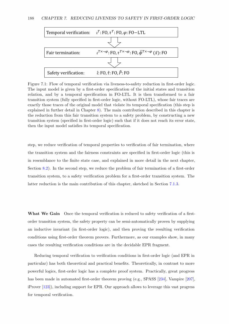
188 CHAPTER 7. REDUCING LIVENESS TO SAFETY IN FIRST-ORDER LOGIC
Temporal verification: 𝜄𝑇: FO, 𝜏𝑇: FO, 𝜑: FO−LTL
Fair termination: 𝜄𝑇׬𝜑: FO, 𝜏𝑇׬𝜑: FO, ത𝜙𝑇׬𝜑 ( ҧ𝑥): FO
Safety verification: Ƹ𝜄: FO, Ƹ𝜏: FO, 𝑃: FO
Figure 7.1: Flow of temporal verification via liveness-to-safety reduction in first-order logic.The input model is given by a first-order specification of the initial states and transitionrelation, and by a temporal specification in FO-LTL. It is then transformed to a fairtransition system (fully specified in first-order logic, without FO-LTL), whose fair traces areexactly those traces of the original model that violate its temporal specification (this step isexplained in further detail in Chapter 8). The main contribution described in this chapter isthe reduction from this fair transition system to a safety problem, by constructing a newtransition system (specified in first-order logic) such that if it does not reach its error state,then the input model satisfies its temporal specification.
step, we reduce verification of temporal properties to verification of fair termination, where
the transition system and the fairness constraints are specified in first-order logic (this is
in resemblance to the finite state case, and explained in more detail in the next chapter,
Section 8.2). In the second step, we reduce the problem of fair termination of a first-order
transition system, to a safety verification problem for a first-order transition system. The
latter reduction is the main contribution of this chapter, sketched in Section 7.1.3.
What We Gain Once the temporal verification is reduced to safety verification of a first-
order transition system, the safety property can be semi-automatically proven by supplying
an inductive invariant (in first-order logic), and then proving the resulting verification
conditions using first-order theorem provers. Furthermore, as our examples show, in many
cases the resulting verification conditions are in the decidable EPR fragment.
Reducing temporal verification to verification conditions in first-order logic (and EPR in
particular) has both theoretical and practical benefits. Theoretically, in contrast to more
powerful logics, first-order logic has a complete proof system. Practically, great progress
has been made in automated first-order theorem proving (e.g., SPASS [234], Vampire [207],
iProver [123]), including support for EPR. Our approach allows to leverage this vast progress
for temporal verification.

7.1. OVERVIEW 189
global nat s, n
local nat m1 2m=n++
[m>s]
3[m≤s]
s++
Figure 7.2: The ticket protocol for mutual exclusion. Threads in state 1 are idle; a thread instate 2 is waiting to enter the critical section; and state 3 is the critical section.
7.1.1 A Running Example
We illustrate our approach using the ticket protocol for ensuring mutual exclusion with
non-starvation among multiple threads, depicted in Figure 7.2. The ticket protocol is an
idealized version of spinlocks used in the Linux kernel [54]. The protocol uses natural numbers
as ticket values. The global state contains a variable, n, that records the next available
ticket, and a variable, s, that records the ticket that is currently being served. Each thread
contains a local ticket variable m. Each thread that wishes to enter the critical section runs
the code depicted in Figure 7.2, where it first acquires a ticket by setting a local variable m
to n and atomically incrementing the next available ticket n. It then waits until its ticket
m is equal to s, the ticket that is served. When this happens, it enters the critical section.
When it exits the critical section, it increases s, allowing the next thread to be served.
We note that the ticket protocol may be run by any number of threads. In fact, the
ticket protocol supports the unbounded-parallelism model, in which new threads may be
created during the run of the protocol. Thus, when considering infinite traces of the ticket
protocol, we cannot assume a finite set of threads, not even an unbounded one. Similarly,
the set of ticket numbers is infinite. The latter is true even if we assume that the number of
threads is finite, since threads may attempt to enter the critical section infinitely often.
7.1.2 First-Order Temporal Specification
We formalize temporal verification problems using first-order transition system specifications
as presented in Section 2.4 to capture the system of interest, and formulas in FO-LTL to
capture temporal specifications. Notice that the FO-LTL specification goes beyond pure
first-order logic, since the semantics of linear temporal logic (where time ranges over the
natural numbers) is not first-order expressible (see e.g., [2]). We now illustrate this formalism
using the ticket example.
In our running example, the formalization of the protocol as a first-order transition
system T t = (Σt,Γt, ιt, τ t) is straightforward, using total orders to abstract the counters
as explained in Chapter 3. The formula for τ t appears in full detail later in this chapter
in Figure 7.4. More interesting is the temporal specification of the ticket protocol, i.e.,

190 CHAPTER 7. REDUCING LIVENESS TO SAFETY IN FIRST-ORDER LOGIC
Liveness Property ∀x : thread. � (pc2(x)→ ♦ pc3(x))
Fairness Assumption ∀x : thread. �♦ scheduled(x)
Temporal Spec. (ϕ) (∀x : thread. �♦ scheduled(x))→ ∀x : thread. � (pc2(x)→ ♦ pc3(x))
¬ϕ (∀x : thread. �♦ scheduled(x)) ∧ (∃x : thread. ♦ (pc2(x) ∧�¬pc3(x)))
Skolem(¬ϕ) (∀x : thread. �♦ scheduled(x)) ∧ ♦ (pc2(t0) ∧�¬pc3(t0))
TSkolem(¬ϕ) ¬q qpc₂(t₀) ∧ ¬pc₃(t₀)
¬pc₃(t₀)φ1(x) = scheduled(x)
φ2 = q
Figure 7.3: Expressing the temporal specification of the ticket protocol. The livenessproperty and fairness assumptions are expressed in FO-LTL. The FO-LTL specification of theprotocol states that the fairness assumptions imply the liveness properties. To obtain a fairtransition system that captures infinite traces that violate the specification, we first negatethe specification and Skolemize the result (t0 is a Skolem constant from the subformula∃x : thread. ♦(pc2(x)∧�¬pc3(x))). We then convert it to the depicted fair transition systemTSkolem(¬ϕ). TSkolem(¬ϕ) has two states, labeled q and ¬q (q is a new nullary relation), andfairness constraints φ1(x), φ2.
non-starvation. Figure 7.3 depicts the FO-LTL specification for the ticket protocol. The
specification we wish to verify is that every thread that requests to enter the critical section
(i.e., reaches location 2), eventually enters (i.e., reaches location 3). This should hold under
the fairness assumption that all the threads are scheduled infinitely often. Thus, the FO-LTL
specification is that the fairness assumption implies liveness. Figure 7.3 also depicts the
negation of the specification, and a “monitor” that tracks it, which we explain next.
Reduction from FO-LTL specification to fair termination As a first step in our
approach for verifying that a transition system given by T = (Σ,Γ, ι, τ) in first-order
logic satisfies a specification given by an FO-LTL formula ϕ, we follow an approach which
generalizes the standard automata theoretic approach from the propositional case to the
first-order case. Specifically, we reduce the problem of verifying a temporal specification for
a transition system, to the problem of checking that a fair transition system has no infinite
fair traces.
A fair transition system is specified by (Σ,Γ, ι, τ, {φ1(x), . . . , φn(x)}), where Σ,Γ, ι, τ
specify the state space, initial states and transitions as usual (see Section 2.4), and each
φi(x) is a first-order formula with free variables, used to specify Buchi acceptance conditions,
which we call fairness constraints. The semantics of the fairness constraints requires that
a fair trace must satisfy each fairness constraint infinitely often, for every assignment to
the free variables. They thus capture infinitely many fairness constraints, for example, that
every thread is scheduled infinitely often.

7.1. OVERVIEW 191
Given a first-order transition system specification T = (Σ,Γ, ι, τ) and an FO-LTL
specification ϕ, we would like to check if T |= ϕ. To reduce this problem to fair termination,
we first negate ϕ and Skolemize it. We then convert the negation of the specification to
a fair transition system, whose fair traces are precisely those that violate ϕ. This can
be done using standard techniques, one of which is presented in Section 8.2. This process
is illustrated for the ticket example in Figure 7.3 (the fair transition system is simplified
for purposes of presentation, but still encodes the correct specification). We then take the
product of the original transition system T , and the transition system that encodes the
negation of ϕ. The result is a fair transition system, whose fair traces are in one-to-one
correspondence to runs of the T that violate ϕ. From this point, all that remains is to check
if the resulting fair transition system is empty or not (i.e., does it have a fair trace). This
reduction to fair termination is both sound and complete.
For the ticket example, the result is a fair transition system with an additional Skolem
constant t0 and an additional nullary relation q that represents the state of an automaton
that is depicted in Figure 7.3, which encodes the negation of the liveness property. The
resulting transition system has two fairness constraints: φ1 = scheduled(x), φ2 = q. Note
that the first constraint has a free thread variable, in order to enforce that every thread is
scheduled infinitely often.
7.1.3 Reducing Fair Termination to Safety
The core result presented in this chapter is a technique for reducing the fair termination
problem of a fair transition system (Σ,Γ, ι, τ, {φ1(x), . . . , φn(x)}) to a safety problem given by
(Σ, Γ, ι, τ) and P , when both systems are specified in first-order logic. This allows standard
methods and other methods developed in this thesis for proving safety to be used.
7.1.3.1 Intuition from the Ticket Protocol Example
Before presenting our reduction, let us gain some intuition from the example of the ticket
protocol. Consider the following intuitive argument that explains why the ticket protocol
satisfies its specification. We need to show that there is no infinite trace in which every
thread is scheduled infinitely often, but at some point it time, say k0, thread t0 takes a
ticket (enters pc2) and from k0 on, t0 never enters the critical section (pc3). We observe that
to show no such trace exists, it suffices to consider the finite set A of threads and ticket
numbers that are active at k0, that is, all threads that were scheduled prior to k0, and all
ticket numbers allocated prior to k0. The reason is that for any interval [k1, k2] later than k0
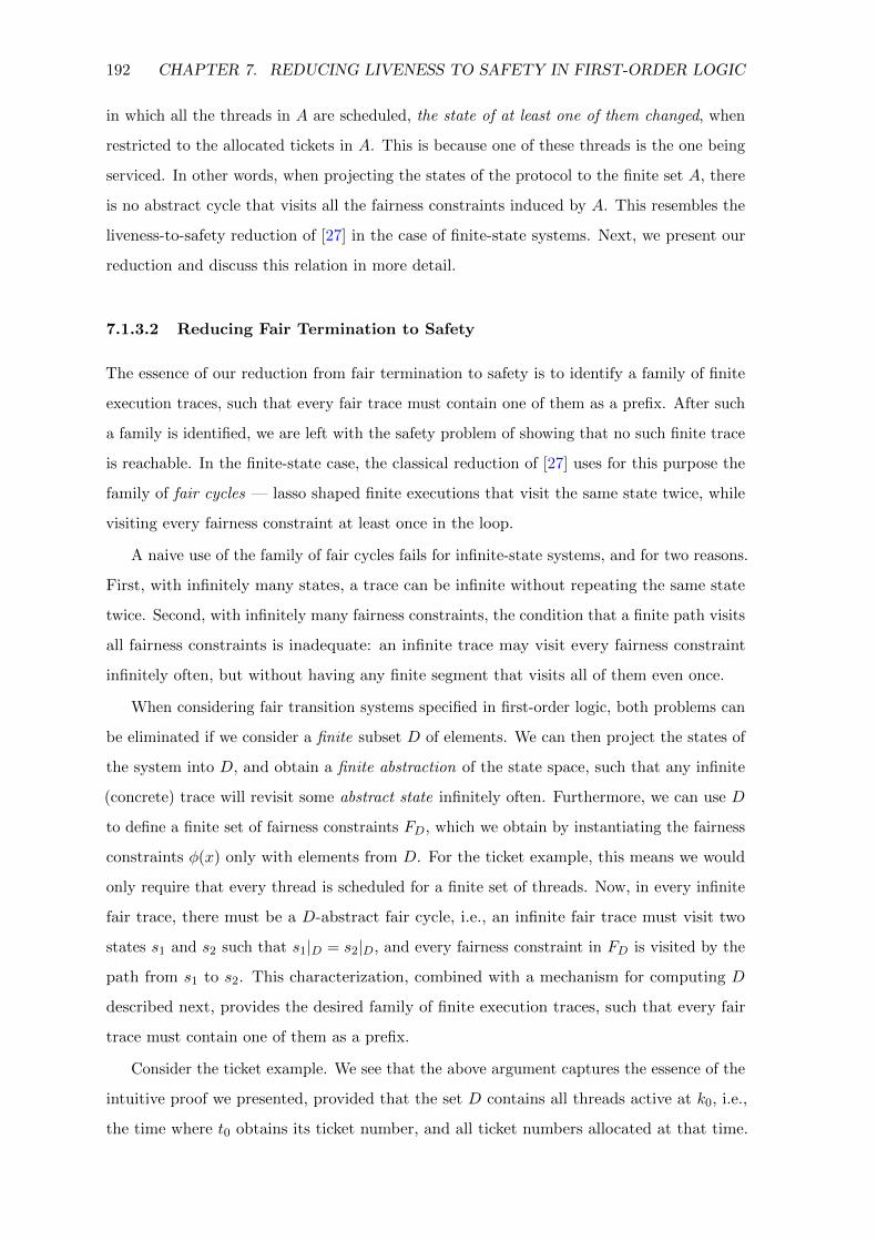
192 CHAPTER 7. REDUCING LIVENESS TO SAFETY IN FIRST-ORDER LOGIC
in which all the threads in A are scheduled, the state of at least one of them changed, when
restricted to the allocated tickets in A. This is because one of these threads is the one being
serviced. In other words, when projecting the states of the protocol to the finite set A, there
is no abstract cycle that visits all the fairness constraints induced by A. This resembles the
liveness-to-safety reduction of [27] in the case of finite-state systems. Next, we present our
reduction and discuss this relation in more detail.
7.1.3.2 Reducing Fair Termination to Safety
The essence of our reduction from fair termination to safety is to identify a family of finite
execution traces, such that every fair trace must contain one of them as a prefix. After such
a family is identified, we are left with the safety problem of showing that no such finite trace
is reachable. In the finite-state case, the classical reduction of [27] uses for this purpose the
family of fair cycles — lasso shaped finite executions that visit the same state twice, while
visiting every fairness constraint at least once in the loop.
A naive use of the family of fair cycles fails for infinite-state systems, and for two reasons.
First, with infinitely many states, a trace can be infinite without repeating the same state
twice. Second, with infinitely many fairness constraints, the condition that a finite path visits
all fairness constraints is inadequate: an infinite trace may visit every fairness constraint
infinitely often, but without having any finite segment that visits all of them even once.
When considering fair transition systems specified in first-order logic, both problems can
be eliminated if we consider a finite subset D of elements. We can then project the states of
the system into D, and obtain a finite abstraction of the state space, such that any infinite
(concrete) trace will revisit some abstract state infinitely often. Furthermore, we can use D
to define a finite set of fairness constraints FD, which we obtain by instantiating the fairness
constraints φ(x) only with elements from D. For the ticket example, this means we would
only require that every thread is scheduled for a finite set of threads. Now, in every infinite
fair trace, there must be a D-abstract fair cycle, i.e., an infinite fair trace must visit two
states s1 and s2 such that s1|D = s2|D, and every fairness constraint in FD is visited by the
path from s1 to s2. This characterization, combined with a mechanism for computing D
described next, provides the desired family of finite execution traces, such that every fair
trace must contain one of them as a prefix.
Consider the ticket example. We see that the above argument captures the essence of the
intuitive proof we presented, provided that the set D contains all threads active at k0, i.e.,
the time where t0 obtains its ticket number, and all ticket numbers allocated at that time.

7.1. OVERVIEW 193
Indeed, for the ticket example, as well as for other interesting examples, one cannot use any
a priori fixed finite set D. A key enabling insight we present is to determine a different D
for different traces, in a way which ensures that for any fair trace, we would assign a finite
set D. In the ticket example, we can define D to be the set of threads scheduled and ticket
numbers allocated prior to k0. A key question is how to determine D in the general case.
Dynamic abstraction and fairness selection using footprint For determining D, we
present a natural solution that is sufficient to fully automate the reduction (i.e., we do not
ask for the user’s help), while being precise enough to capture challenging examples. Our
solution is to maintain a finite set of elements that is the footprint of a finite execution prefix.
Transitions are usually local, in the sense that each transition affects (and is affected by)
a finite set of elements. We show that we can syntactically extract this finite set from the
transition relation τ . For the ticket example, the footprint of a prefix would precisely be all
the threads scheduled, and all the ticket numbers allocated.
This gives rise to a natural way to define D. Given a trace, wait for a time k0 when a
certain condition is met, and then let D be the footprint of the execution prefix up to k0. In
the ticket example, a suitable condition is that thread t0 obtains its ticket number. In the
general case, we must choose a condition such that every infinite fair trace eventually meets
it. Our canonical solution for this is to wait for a finite subset of the fairness constraints,
which is determined by the initial state. In particular, it will include all nullary fairness
constraints, i.e., fairness constraints given by formulas without free variables. For the ticket
example, φ2 = q is a nullary fairness constraint, ensuring that k0 is after t0 obtains its ticket
number. This works well for other interesting examples as well.
Realization of the reduction With these definitions ofD and k0, we define an algorithmic
reduction of fair termination to safety in first-order logic. Given a fair first-order transition
system, the reduction augments it by a monitor that identifies finite execution traces that
(1) reach the point k0 in which D is set to the footprint of the execution so far, and (2)
afterwards visit two states s1 and s2 such that s1|D = s2|D and every fairness constraint in
FD is visited by the path from s1 to s2. Upon identifying such a prefix, the monitor enters
an error state. The output of the reduction is the augmented transition system and the
safety property that the error state is not reachable.
Note that, while the soundness of our reduction relies on a notion of a dynamic finite
abstraction, we do not construct an abstract transition system. In fact, the reduction does
not incur any abstraction of the transitions. The finite abstraction is only used by the

194 CHAPTER 7. REDUCING LIVENESS TO SAFETY IN FIRST-ORDER LOGIC
monitor that augments the transition system, for abstract fair cycle detection.
Parameterized systems Parameterized systems are a special case of infinite-state systems,
where each value of the parameter defines a finite-state instance of the system, but the
parameter itself is unbounded. In first-order logic, this means we are only interested in traces
over finite domains. In this case, it is sound to prove fair termination by proving the absence
of fair cycles. This can be viewed as a special case of our approach, where the footprint
includes all elements of the domain. Note that for this setting, the reduction to safety is
complete, i.e., if the original transition system has no infinite fair traces, then the resulting
system will be safe. While our main interest here is in systems that are truly infinite-state,
it is nice to note that our general formalism maintains completeness in the special case of
parameterized systems.
7.1.4 A Nested Termination Argument
For finite-state systems and for parameterized transition systems the reduction from fair
termination to fair cycle detection is complete. For infinite-state systems the reduction we
present is sound but not complete. This is expected, since fair termination is theoretically
harder than safety1. Incompleteness of the reduction means that for some instances where
the input system has no fair traces, the output system will not be safe. While incompleteness
is unavoidable, we would like a reduction that works for examples of interest. However, the
reduction presented in the previous section fails for a particular class of natural examples.
Intuitively, this happens when progress is not obtained in a bounded number of steps
after we fix the finite set of elements used for abstract fair cycle detection. To handle such
examples, we develop a more powerful reduction that relies on a nesting structure provided
by the user. A nesting structure divides the transitions of a system into several nested levels.
Given such a structure, one can use abstract fair cycle detection for each level separately,
while assuming subsequent levels terminate.
7.2 Preliminaries
In this section we extend the formalism presented in Chapter 2 to temporal specifications
using FO-LTL. We also present the fair transition systems in first-order logic, the analog of
(generalized) Buchi automata for first-order transition systems.
1For transition systems in first-order logic, it is easy to show that fair termination is Π11 hard (see [2]),
while safety is in the arithmetical hierarchy.

7.2. PRELIMINARIES 195
7.2.1 First-Order Linear Temporal Logic (FO-LTL)
To specify temporal properties of first-order transition systems we use First-Order Linear
Temporal Logic (FO-LTL), which combines LTL with first-order logic (see e.g., [2]). For
simplicity of presentation, we consider only the “globally” (�) and the “eventually” (♦)
temporal operators. Our approach also extends to other standard temporal operators (i.e.,
“next” and “until”).
Syntax Given a first-order vocabulary Σ, FO-LTL formulas are defined by:
f ::= r(t1, . . . , tn) | t1 = t2 | ¬f | f1 ∨ f2 | ∃x.f | �f
where r is an n-ary relation symbol in Σ, x is a variable, each ti is a term over Σ (defined
as in first-order logic) and � denotes the “globally” temporal operator. We also use the
standard shorthand for the “eventually” temporal operator: ♦f = ¬�¬f , and the usual
shorthands for logical operators (e.g., ∀x.f = ¬∃x.¬f).
Semantics FO-LTL formulas over Σ are interpreted over infinite sequences of states
(first-order structures) over Σ, with the same domain D. Atomic formulas are interpreted
over states (which are first-order structures), the temporal operators are interpreted as in
traditional LTL, and first-order quantifiers are interpreted over the shared domain D.
Formally, the semantics is defined w.r.t. an infinite sequence of states π = s0, s1, . . .
and an assignment σ that maps variables to D — the shared domain of all states in π. We
sometimes omit σ when the formula has no free variables. We define πi = si, si+1, . . . to be
the suffix of π starting at index i. The semantics is defined as follows.
π, σ |= r(t1, . . . , tn)⇔ s0, σ |= r(t1, . . . , tn)
π, σ |= t1 = t2 ⇔ s0, σ |= t1 = t2
π, σ |= ¬ψ ⇔ π, σ 6|= ψ
π, σ |= ψ1 ∨ ψ2 ⇔ π, σ |= ψ1 or π, σ |= ψ2
π, σ |= ∃x.ψ ⇔ exists d ∈ D s.t. π, σ[x 7→ d] |= ψ
π, σ |= �ψ ⇔ forall i ≥ 0, πi, σ |= ψ
We say that a first-order transition system (Σ,Γ, ι, τ) satisfies a closed FO-LTL formula
ϕ over Σ if all of its traces satisfy ϕ (i.e., for every D).

196 CHAPTER 7. REDUCING LIVENESS TO SAFETY IN FIRST-ORDER LOGIC
Σt = {n : ticket, s : ticket,m : thread→ ticket,≤ (ticket, ticket), pc1(thread), pc2(thread), pc3(thread), scheduled(thread)}Γt = {ψtotal order}ιt = ψmin(n) ∧ ψmin(s) ∧ ∀x : thread. pc1(x) ∧ ¬pc2(x) ∧ ¬pc3(x) ∧ ψmin(m(x)) ∧ ¬scheduled(x)
τ t = ∃x : thread. τ(x)
τ(x) = (τ12(x) ∨ τ22(x) ∨ τ23(x) ∨ τ31(x)) ∧ ∀y : thread.scheduled ′(y)↔ x = y
τ12(x) = ψ12(x) ∧m′(x) = n ∧ (∀y : thread. x 6= y → m ′(y) = m(y)) ∧ ψsucc(n, n′) ∧ s′ = s
τ22(x) = ψ22(x) ∧m(x) > s ∧ (∀y : thread. m ′(y) = m(y)) ∧ n′ = n ∧ s′ = s
τ23(x) = ψ23(x) ∧m(x) ≤ s ∧ (∀y : thread. m ′(y) = m(y)) ∧ n′ = n ∧ s′ = s
τ31(x) = ψ31(x) ∧ (∀y : thread. m ′(y) = m(y)) ∧ n′ = n ∧ ψsucc(s, s′)
ψij(x) = pci(x) ∧ pc′j(x) ∧(∧
k 6=j ¬pc′k(x))∧∧
k ∀y : thread. x 6= y → (pc′k(y)↔ pck(y))
ψmin(x) = ∀y : ticket. x ≤ yψsucc(x, y) = x < y ∧ ∀z : ticket. x < z → y ≤ zψtotal order = (∀x : ticket. x ≤ x) ∧ (∀x, y, z : ticket. x ≤ y ∧ y ≤ z → x ≤ z)∧
(∀x, y : ticket. x ≤ y ∧ y ≤ x→ x = y) ∧ (∀x, y : ticket. x ≤ y ∨ y ≤ x)
Figure 7.4: First-order logic specification of the ticket protocol. The vocabulary includesuninterpreted relations and functions, and a total order on ticket values ≤, axiomatized byψtotal order.
7.2.2 Fair Transition Systems
A (Buchi) fair transition system is a tuple (S, S0, R,F) where (S, S0, R) are a usual transition
system (as in Section 2.3), and F ⊆ P (S) is a (possibly infinite) set of fairness constraints.
An infinite trace π = s0, s1, . . . is fair if it visits every fairness constraint F ∈ F infinitely
often, i.e., for every F ∈ F the set {i | si ∈ F} is infinite.
Fair termination The fair transition system (S, S0, R,F) terminates if it has no fair
(infinite) traces.
Specification in first-order logic As usual, we specify transition systems in first-order
logic, by providing (Σ,Γ, ι, τ). As an example, Figure 7.4 depicts the first-order logic
specification of the ticket protocol. In this chapter, we simplify the formal presentation by
handling only relations and constant symbols from the vocabulary, as function symbols can
be treated as special relations with increased arity.
A first-order logic specification of a fair transition system is (Σ,Γ, ι, τ,Φ), where Σ,Γ, ι, τ
are as usual, and Φ = {φ1, . . . , φn}, where each φi is a formula over Σ that may contain
free variables. For each domain D, the semantics of (Σ,Γ, ι, τ,Φ) is a fair transition system
(S, S0, R,F) where S, S0, R are as usual, and F is a possibly infinite set of fairness constraints

7.2. PRELIMINARIES 197
defined by Φ:
F = {Fφ(e) | φ(x1, . . . , xn) ∈ Φ, e ∈ Dn}
where Fφ(e) = {s ∈ S | s, [x1 7→ e1, . . . , xn 7→ en] |= φ(x1, . . . , xn)}
Note that each fairness formula φ ∈ Φ with free variables induces a set of fairness constraints
of the form Fφ(e), for each e ∈ Dn. Observe that since D may be infinite, φ may stand for
infinitely many such fairness constraints.
We say that (Σ,Γ, ι, τ,Φ) terminates if it has no fair (infinite) traces, i.e., if for any D,
the fair transition system defined for D terminates.
7.2.3 Reducing FO-LTL Verification to Fair Termination
Given any closed formula f in FO-LTL over vocabulary Σ, we can construct a fair transition
system (monitor) over an extended vocabulary Σf ⊇ Σ such that the pointwise-projection of
its set of fair traces on Σ is exactly the set of all traces that satisfy f . This is a straightforward
extension of the classical construction of a Buchi automaton for an LTL formula used in the
automata theoretic approach to verification [233, 236], except that instead of a finite-state
automaton we obtain a fair first-order transition system. We defer explaining this in detail
to Section 8.2 in the next chapter.
To check whether a given transition system (Σ,Γ, ι, τ) satisfies f we can then take
the product of the “monitor” of ¬f and the original transition system. Proving that the
original transition system satisfies the FO-LTL formula f reduces to proving that the product
transition system has no fair traces. This reduction is sound and complete, meaning that
(Σ,Γ, ι, τ) satisfies f if and only if the fair transition system terminates. As such, from
now on we focus on proving fair termination. This allows us to verify arbitrary FO-LTL
properties.
7.2.3.1 Illustration on the Ticket Protocol
Consider the first-order logic specification of the ticket protocol, (Σt,Γt, ιt, τ t), presented in
Figure 7.4. Its desired FO-LTL specification, and the steps of constructing a monitor for its
negation are presented in Figure 7.3. The constructed monitor is a fair transition system,
defined over vocabulary {pc2(thread), pc3(thread), scheduled(thread), t0 : thread, q}. We
compose it with the transition system of the ticket protocol. The result is a fair transition
system (Σ,Γ, ι, τ,Φ) defined below, whose fair (infinite) traces represent traces of the protocol

198 CHAPTER 7. REDUCING LIVENESS TO SAFETY IN FIRST-ORDER LOGIC
waitingW := µ(s)
W := W \ {F ∈ ℱ | s ∈ F}
frozen
[W=∅]A := α(s) saved
t := sW := µ(s)
W := W \ {F ∈ ℱ | s ∈ F}
error[W=∅∧A(t)=A(s)]
Figure 7.5: Monitor that checks the (α, µ)-acyclicity condition. The monitor uses auxiliarystate: W ∈ Pfin (F), A : S → X, and t ∈ S. The variable s denotes the current state of themonitored transition system. W is a finite set of fairness constraints for which the monitor iswaiting. A is used to store α(skf ), and t is used to store sk1 (see Definition 7.8). The monitorstarts with an initial condition that W is µ(s0), and then goes into waiting state, in which itupdates W by removing fairness constraints that have been satisfied. Once W = ∅, a fairprefix is obtained, hence the monitor non-deterministically decides whether kf is reached, inwhich case it freezes the abstraction by setting A to α(skf ). It then non-deterministicallychooses when to fix k1. When this happens, the monitor saves sk1 in t, and also resets Wto µ(sk1). It then keeps updating W , and checks if we reach a point in which W = ∅ andA(t) = A(s), i.e., a point k2 s.t. [k1, k2] is µ-fair, and α(skf )(sk1) = α(skf )(sk2). If thishappens, the monitor goes to the error state. The error state is thus reachable in the productof the monitor with the transition system if and only if the (α, µ)-acyclicity condition isviolated.
that violate the specification, hence its fair termination implies correctness of the protocol:
Σ = Σt ∪ {t0 : thread, q}
Γ = Γt
ι = ιt ∧ ¬q
τ = ∃x : thread. τ(x) ∧ t′0 = t0 ∧ τq
where τq = (¬q ∧ ¬q′) ∨ (¬q ∧ q′ ∧ pc′2(t0) ∧ ¬pc′3(t0)) ∨ (q ∧ q′ ∧ ¬pc′3(t0))
Φ = {φ1(x), φ2} where φ1(x) = scheduled(x), φ2 = q
7.3 Reducing Fair Termination to Safety in First-Order Logic
In this section we introduce our approach for proving fair termination using first-order logic.
The approach is based on a reduction from fair termination to safety that is applied to
transition systems in first-order logic. We start by presenting the reduction parameterized
by a dynamic abstraction function and a fairness selection function, and establishing its
soundness. Next, we show how to apply the reduction using first-order logic, by defining a
canonical dynamic abstraction and fairness selection functions.

7.3. REDUCING FAIR TERMINATION TO SAFETY IN FIRST-ORDER LOGIC 199
7.3.1 Parametric Reduction via Dynamic Abstraction
For clarity of the presentation, we first present the reduction of fair termination to safety in a
semantic way, ignoring the first-order logic aspects. This semantic reduction is parameterized
by a dynamic finite abstraction function, and a dynamic fairness selection function (defined
below). In Section 7.3.2, we show how to algorithmically derive these functions for transition
systems that are specified in first-order logic.
Fix a fair transition system (S, S0, R,F). Roughly speaking, the termination argument
for proving that (S, S0, R,F) has no fair traces is based on showing that no fair abstract
cycle exists. To ensure soundness of this argument, we use a dynamic finite abstraction
function that must abstract states into a finite set, and we use a dynamic fairness selection
function that must select a finite set of fairness constraints, to ensure that eventually they
are all satisfied in a finite trace (facilitating the existence of a fair abstract cycle). Formally:
Definition 7.6 (Dynamic Finite Abstraction). A dynamic finite abstraction function is a
function α : S → S → X, where X is any set, and for any s ∈ S the range of α(s) is finite.
Definition 7.7 (Dynamic Fairness Selection). A dynamic fairness selection function is a
function µ : S → Pfin (F) (where Pfin (F) denotes the set of finite subsets of F). Given a
trace (either infinite or finite) π = s0, s1, . . . and 0 ≤ k < k′ < |π|, we say that the [k, k′]
segment of π is µ-fair if ∀F ∈ µ(sk). {sk+1, . . . , sk′−1} ∩ F 6= ∅.
Recall that we consider transition systems with infinitely many fairness constrains. (In
first-order logic transition systems, the fairness formulas induce infinitely many fairness
constraints, by instantiating the free variables.) In this setting, an infinite trace can be
fair without containing any finite segment that visits all fairness constraints. The dynamic
fairness selection function is therefore used to select a finite subset of the fairness constraints
that is “relevant” for a particular state (note that each fairness constraint that is selected for
µ(s) is taken as a whole from F ; that is, µ does not change the individual fairness constraints,
and only selects finitely many fairness constraints for each state). Note that in an infinite
fair trace, for every k there exists a k′ > k such that the [k, k′] segment is µ-fair.
To prove that (S, S0, R,F) has no fair traces, we require a dynamic finite abstraction
function α and a dynamic fairness selection function µ such that there are no (α, µ)-abstract
fair cycles, as defined below.
Definition 7.8 ((α, µ)-Abstract Fair Cycle). A finite trace s0, s1, . . . , sn contains an (α, µ)-
abstract fair cycle if there are kf < k1 < k2 ≤ n such that the segments [0, kf ] and [k1, k2]

200 CHAPTER 7. REDUCING LIVENESS TO SAFETY IN FIRST-ORDER LOGIC
are µ-fair, and we have α(skf )(sk1) = α(skf )(sk2). The (α, µ)-acyclicity condition requires
that no trace contains an (α, µ)-abstract fair cycle.
Intuitively, the acyclicity condition requires that any fair segment [k1, k2] that follows a
fair prefix [0, kf ] cannot form a cycle when states are abstracted by the finite abstraction
associated with skf . The index kf can therefore be viewed as the “freeze” point of the finite
abstraction, after which no fair abstract cycle is allowed. Note that the condition requires
that no matter which freeze point is selected (as long as the prefix [0, kf ] is µ-fair), the finite
abstraction α(skf ) is precise enough to exclude a fair abstract cycle.
Lemma 7.9. Let (S, S0, R,F) and α and µ be s.t. the (α, µ)-acyclicity condition is satisfied,
then (S, S0, R,F) has no fair traces.
Proof. Assume to the contrary that (sk)∞k=0 is a fair trace of (S, S0, R,F). Let kf be an
index such that the [0, kf ] segment is µ-fair. Consider the sequence(α(skf )(sk)
)∞k=0
. Since
the range of α(skf ) is finite, there must be an infinite subsequence that consists of a constant
x ∈ X. Let k1 ≥ kf be the index of the first occurrence of x after kf . Due to fairness,
there must exist k2 > k1 such that the [k1, k2] segment is µ-fair. The reason is that a fair
trace must visit every element of F infinitely often. This ensures that whenever we fix k1
and select the finite subset of F given by µ(sk1), we will encounter all elements of µ(sk1)
after some finite number of transitions. In particular, this segment can be extended such
that α(skf )(sk2) = x (since x repeats infinitely often), i.e., α(skf )(sk1) = α(skf )(sk2). This
contradicts the acyclicity condition.
Monitoring the (α, µ)-acyclicity condition Since an (α, µ)-abstract fair cycle is mani-
fested in a finite prefix of the trace, the (α, µ)-acyclicity condition (Definition 7.8) is a safety
property of (S, S0, R,F). Hence, given α and µ, Lemma 7.9 lets us reduce fair termination
to safety checking.
The safety property can be further simplified by creating a monitor that checks the
presence of (α, µ)-abstract fair cycles. Figure 7.5 presents such a monitor that is parameterized
by α and µ. The monitor runs in parallel to the transition system and tracks violations
of the (α, µ)-acyclicity condition, i.e., presence of (α, µ)-abstract fair cycles. That is, the
monitor checks for the presence of a trace s0, s1, . . . of (S, S0, R,F) where for some kf the
segments [0, kf ] and [k1, k2] are µ-fair but α(skf )(sk1) = α(skf )(sk2). To identify the µ-fair
prefix [0, kf ], the monitor starts in state “waiting” and uses a set W ∈ Pfin (F) of fairness
constraints that is initialized to µ(s0); while the monitor is in state “waiting”, W is updated
whenever the current state s of the monitored transition system visits one of the fairness

7.3. REDUCING FAIR TERMINATION TO SAFETY IN FIRST-ORDER LOGIC 201
constraints. When W = ∅, the prefix is µ-fair, hence the monitor non-deterministically selects
the “freeze” point kf and stores the corresponding finite abstraction α(skf ) in A : S → X. It
then moves to state “frozen” from which it non-deterministically selects k1, where it saves sk1
in t ∈ S and initializes W to µ(sk1) in order to identify a µ-fair segment. It then continues
to state “saved” where it updates W in each step, and when W = ∅, i.e., [k1, k2] is a µ-fair
segment, if a state s is encountered where A(s) = A(t), then the monitor goes to state “error”
and declares violation.
Clearly, the error state is reachable in the product of the monitor with the transition
system if and only if the (α, µ)-acyclicity condition is violated. Therefore, the reduction from
fair termination to safety constructs the product of the monitor with the transition system.
Fair termination then reduces to checking that the product transition system, denoted
(S, S0, R), satisfies the safety property P¬error defined by the set of states where the monitor
is not in its error state. Note that the product transition system has no fairness constraints,
since we are only interested in its safety (i.e., in its finite traces). We also note that (S, S0, R)
is not an abstract transition system. The use of the dynamic finite abstraction α does not
incur any abstraction of the transitions, and it is only used for checking the (α, µ)-acyclicity
condition.
Lemma 7.10. Let (S, S0, R,F) be a transition system, α a dynamic finite abstraction
function and µ a dynamic fairness selection function, and let (S, S0, R) be the transition
system obtained from the composition of (S, S0, R) with the (α, µ)-acyclicity monitor specified
in Figure 7.15. If (S, S0, R) satisfies the safety property P¬error, then (S, S0, R,F) has no
fair traces.
7.3.2 Uniform Reduction in First-Order Logic
We now present the realization of the reduction for a first-order transition system T =
(Σ,Γ, ι, τ,Φ). The main ingredients are the algorithmic extraction of a dynamic finite
abstraction function α and a fairness selection function µ based on the footprint of a trace,
and the realization of the acyclicity monitor based on these functions as a transition system
in first-order logic.
Tracking the footprint of a trace The dynamic finite abstraction and fairness selection
functions formalized in the previous section rely on finiteness arguments. The first key idea
that allows us to realize these functions in first-order logic is to augment the first-order
transition system (Σ,Γ, ι, τ,Φ) with a new unary relation d that will always contain a finite

202 CHAPTER 7. REDUCING LIVENESS TO SAFETY IN FIRST-ORDER LOGIC
number of elements, and will intuitively accumulate all the elements that the trace has seen
or affected so far.
Assume, without loss of generality, that ι and τ are given in the following form:
ι = ∃x1, . . . , xn. ι(x1, . . . , xn) τ = ∃x1, . . . , xm. τ(x1, . . . , xm)
Then, define an augmented transition system (Σd,Γd, ιd, τd,Φd) where
Σd = Σ ∪ {d1}
Γd = Γ
ιd = ∃x1, . . . , xn. ι ∧ ∀x. d(x)↔(∨n
i=1 x = xi ∨∨c∈Σ x = c
)τd = ∃x1, . . . , xm. τ ∧ ∀x. d′(x)↔
(d(x) ∨∨m
i=1 x = xi ∨∨c∈Σ x = c′
)Φd = Φ
Intuitively, the d relation contains the elements that affect or are affected by the transition,
captured by the existentially quantified variables and constants. For both sequential programs
and distributed algorithms, each transition usually interacts with a finite set of elements
(e.g., threads, memory locations, values, etc.). This set is sometimes called the footprint of
a transition. The idea of d is that it is updated so that it includes the footprint of all the
transitions in the trace so far.
The augmentation of the transition system with d has two benefits, captured by the
following lemmas. First, it does not affect termination:
Lemma 7.11. (Σd,Γd, ιd, τd,Φd) terminates if and only if (Σ,Γ, ι, τ,Φ) terminates.
Second, it provides a way to select a finite set of elements in each reachable state:
Lemma 7.12. Let s = (D, I) be a reachable state of (Σd,Γd, ιd, τd,Φd). Then the interpre-
tation of d, I(d) ⊆ D, is a finite set.
The reason is that d initially contains at most n+ |C| elements, and with each transition
it grows by at most m+ |C| elements, where C denotes the set of constant symbols in Σ.
Dynamic finite abstraction and fairness selection functions based on footprints
Now, we apply the reduction from fair termination to safety on (Σd,Γd, ιd, τd,Φd). To do so,
we define the finite abstraction function for (Σd,Γd, ιd, τd,Φd) by projecting all relations to
the finite set given by d (at kf ), and we define the fairness selection function by taking all

7.3. REDUCING FAIR TERMINATION TO SAFETY IN FIRST-ORDER LOGIC 203
the fairness constraints over all elements of d. Given an interpretation I and a set A, define
the projection of I to A as I|A = λr. I(r) ∩ Aarity(r). Observe that if A is finite, then the
range of λI.I|A is finite. For s = (D, I), define s|A = (A, I|A).
Definition 7.13 (First-order α and µ). For any state s = (D, I) of (Σd,Γd, ιd, τd,Φd), let
α(s) = λs′. s′|I(d)
µ(s) = {Fφ(e) | φ(x1, . . . , xn) ∈ Φ, e ∈ (I(d))n} see Section 7.2 for the definition of Fφ(e)
Since I(d) is finite, the range of α(s) is finite, and so is µ(s)2.
Implementing the acyclicity monitor in first-order logic Having defined the dy-
namic finite abstraction function α and the fairness selection function µ, in order to complete
the reduction of fair termination to safety it remains to implement the monitor presented in
Figure 7.5 for α and µ in first-order logic, and compose it with (Σd,Γd, ιd, τd,Φd).
Figure 7.15 presents the realization of the monitor in first-order logic, using a vocabulary
Σm ⊇ Σd which we describe next. The control states of the monitor are tracked using nullary
relations waiting, frozen, saved, error ∈ Σm. The key ideas are to “freeze” the abstraction
at kf by copying the relation d ∈ Σd at the freeze point into an auxiliary unary relation
a ∈ Σm, and to “select” the relevant subset of the fairness constraints (both initially and
when moving to the “saved” state) by introducing an auxiliary relation wi ∈ Σm for each
quantified fairness constraint φi and initializing it to all tuples in d. To implement the check
whether A(t) = A(s) (indicating that an abstract state is repeated), the monitor remembers t
by introducing a copy Σs = {as | a ∈ Σ} of Σ which is set when moving to the “saved” state.
Then, the equality of the abstract states is checked by comparing the relation and constant
symbols in Σs (representing the old state t) and their counterparts in Σ (representing the
current state s) on the elements in a. This mimics applying the projection which defines the
abstraction at kf . We denote the first-order specification of the monitor by (Σm, ιm, τm).
The product of (Σd,Γd, ιd, τd,Φd) with the monitor is then the first-order transition
2 Strictly speaking, this is only true for the reachable states of (Σd,Γd, ιd, τd), since there are unreachablestates in which d contains infinitely many elements. However, the soundness result is unaffected by this, sincethe proof of Lemma 7.9 only applies α and µ to reachable states.

204 CHAPTER 7. REDUCING LIVENESS TO SAFETY IN FIRST-ORDER LOGIC
cmd first-order realization
W := µ(s)∧
i ∀x. w′i(x)↔ ∧
j d(xj)
W := W \ {F ∈ F | s ∈ F} ∧i ∀x. w′
i(x)↔ (wi(x) ∧ ¬φi(x))
[W = ∅] ∧i ∀x. ¬wi(x)
A := α(s) ∀x. a′(x)↔ d(x)
t := s∧
r∈Σ ∀x. r′s(x)↔ r(x) ∧ ∧c∈Σ c′s = c
[A(t) = A(s)]∧
r∈Σ ∀x.(∧
j a(xj))→ (rs(x)↔ r(x)) ∧∧c∈Σ(a(c) ∨ a(cs))→ c = cs
Figure 7.15: Realization in first-order logic of commands from Figure 7.5. The first-orderlogic realization uses the following relations: wi for each φi ∈ Φ (wi has the same arity asφi), to implement W ; a unary relation a, capturing A by recording the interpretation of d atkf ; a relation rs for every r ∈ Σ (with the same arity), to implement t and capture a copy ofthe interpretation of all state relations at k1.
system (without fairness constraints) T = (Σ, Γ, ι, τ), where
Σ = Σm = Σd ∪ Σs ∪ {waiting, frozen, saved, error, a} ∪ {wi | φi ∈ Φ}
Γ = Γd = Γ
ι = ιd ∧ ιm
τ = τd ∧ τm
The following theorem summarizes the reduction from fair termination to safety in
first-order logic, as well as its correctness:
Theorem 7.14. Let T = (Σ,Γ, ι, τ,Φ) be a fair transition system in first-order logic, and
let T = (Σ, Γ, ι, τ) be the transition system defined above. If T satisfies the safety property
P = ¬error, then T has no fair traces.
The reduction from fair termination to safety is linear (both in time and space) in the size
of (the description of) T . The size of (the description of) the resulting first-order transition
system T is approximately twice as big as that of T (due to the copied relations).
Handling finite domains In some settings, we have additional knowledge that some
sets of elements are always finite. For example, we could be interested in a distributed or
multithreaded protocol without unbounded-parallelism. That is, we consider the protocol
only when it is running on a fixed, finite (albeit unbounded) set of nodes or threads. Such a
protocol can still use some infinite sorts representing integer values, messages, etc. In such
a setting, we may include all threads, nodes, or any other set that is known to be finite
into the initial condition for d. Another example is where we might include all elements
smaller than some constant representing a natural number initially in d. The soundness of

7.3. REDUCING FAIR TERMINATION TO SAFETY IN FIRST-ORDER LOGIC 205
the reduction is maintained, as long as d is guaranteed to be finite in all reachable states.
In particular, in the case of parameterized systems, where all the sorts are finite, we can
include all elements of the domain in the initial condition of d, while preserving soundness of
the reduction. In fact, in this case, fair cycle detection is sound without any abstraction nor
fairness selection. Thus, the transition system of the monitor can be simplified by eliminating
both d and a, and starting the monitor in the “frozen” state, while initializing W to contain
all fairness constraints, and including all elements in the cycle detection (instead of just the
ones in a).
Using derived relations and ghost code to increase precision Our dynamic abstrac-
tion of a state is computed completely automatically by projecting the first-order structure
to the set of elements determined by the footprint I(d) at the freeze point. The precision of
the abstraction can thus be increased by using additional derived relations, which can allow
the projection to distinguish between more states. For example, consider a vocabulary with a
unary relation r. Suppose that two states, s1 and s2, differ in their interpretation of r, where
I1(r) = ∅ and I2(r) = {e}, but e is not included in the finite set by which the abstraction
is computed. In this case, α(sf )(s1) = s1|If (d) = s2|If (d) = α(sf )(s2). However, if we add
to the vocabulary a nullary derived relation r′ that tracks the formula ∃x. r(x), then we
will now have that α(sf )(s1) 6= α(sf )(s2), due to the different interpretation of r′. We used
such derived relations for the liveness verification of Paxos protocols (see Section 7.6.1).
Another possible way to increase the precision of the abstraction is by adding ghost code
that increases the footprint of transitions. This will also cause the finite set of elements to
which we project to be larger, making the abstraction more precise.
7.3.3 Detailed Illustration for Ticket Protocol
We now illustrate our reduction of fair termination to safety on the ticket protocol. Let
(Σ,Γ, ι, τ,Φ) be the fair transition system defined in Section 7.2.3.1 for the ticket protocol.
To prove the fair termination of (Σ,Γ, ι, τ,Φ) we apply our reduction to safety. The first step
is to augment the transition system by tracking the footprint. This results in the following
transition system, T d (note that we add a unary relation for each sort):

206 CHAPTER 7. REDUCING LIVENESS TO SAFETY IN FIRST-ORDER LOGIC
Σd = Σ ∪ {dthread(thread), dticket(ticket)}
Γd = Γt
ιd = ι ∧ (∀x : thread. dthread(x)↔ (x = t0)) ∧ (∀x : ticket. dticket(x)↔ (x = n ∨ x = s))
τd = ∃x : thread. τ(x) ∧ t′0 = t0 ∧ τq ∧(∀y : thread. d′thread(y)↔ (dthread(y) ∨ x = y)
)∧(
∀y : ticket. d′ticket(y)↔ (dticket(y) ∨ y = n′ ∨ y = s′))
Next, we construct the first-order realization of the monitor of Figure 7.5 and compose it
with the augmented transition system. This completes the reduction from fair termination
to safety reduction, and results in the following transition system, T :
Σ = Σd ∪ {rs | r ∈ Σ} ∪ {waiting , frozen, saved , error}
∪ {athread(thread), aticket(ticket), w1(thread), w2}
Γ = Γd = Γt
ι = ιd ∧ waiting ∧ ¬frozen ∧ ¬saved ∧ ¬error ∧ (∀x : thread. w1(x)↔ dthread(x)) ∧ w2
τ = τd ∧ (τwait ∨ τfreeze ∨ τsave ∨ τerror)
τwait = (waiting ′ ↔ waiting) ∧ (frozen ′ ↔ frozen) ∧ (saved ′ ↔ saved)∧(∀x : thread. w′1(x)↔ (w1(x) ∧ ¬scheduled(x))
)∧ (w′2 ↔ (w2 ∧ ¬q))
τfreeze = waiting ∧ ¬waiting ′ ∧ frozen ′ ∧ ¬saved ′ ∧ (∀x : thread. ¬w1(x)) ∧ ¬w2 ∧(∀x : thread. a′thread(x)↔ dthread(x)
)∧(∀x : ticket. a′ticket(x)↔ dticket(x)
)τsave = frozen ∧ ¬waiting ′ ∧ ¬frozen ′ ∧ saved ′ ∧
(∀x : thread. w′1(x)↔ dthread(x)
)∧ w′2 ∧
n′s = n ∧ s′s = s ∧ q′s ↔ q ∧ ∀x : thread. m′s(x) = m(x) ∧∧
kpck′s(x)↔ pck(x)
τerror = saved ∧ error ′ ∧ (∀x : thread. ¬w1(x)) ∧ ¬w2 ∧ qs ↔ q ∧(∀x : thread. athread(x)→
∧k
pcks(x)↔ pck(x))∧
(∀x : ticket. aticket(x)→ (ns = x↔ n = x) ∧ (ss = x↔ s = x))∧
(∀x : thread, y : ticket. athread(x) ∧ aticket(y)→ (ms(x) = y ↔ m(x) = y))
Inductive invariant To provide a better understanding of the entire verification process,
we discuss the inductive invariant that establishes the safety of the system T that results
from the reduction for the example of the ticket protocol. The inductive invariant includes

7.4. CAPTURING NESTED TERMINATION ARGUMENTS 207
some rather straightforward properties of reachable states of the ticket protocol. The most
interesting part of the inductive invariant is the one that establishes the connection between
the protocol state and the footprint, as well as the absence of fair abstract cycles. This part
is:
∀x : thread. (pc2(x) ∨ pc3(x))→ dthread(x)
∀x : ticket. x ≤ n→ dticket(x)
(frozen ∨ saved)→ ∀x : thread. (pc2(x) ∨ pc3(x)) ∧m(x) ≤ m(t0)→ athread(x)
(frozen ∨ saved)→ ∀x : ticket. x ≤ m(t0)→ aticket(x)
∀x : ticket. s ≤ x < n→ ∃y : thread. m(y) = x ∧ (pc2(y) ∨ pc3(y))
saved → ∀x : thread. (ms(x) = ss ∧ pc2s(x) ∧ ¬w1(x))→
((pc1(x) ∧m(x) = ss) ∨ (pc2(x) ∧m(x) > m(t0)) ∨ (pc3(x) ∧m(x) = ss))
saved → ∀x : thread. (ms(x) = ss ∧ pc3s(x) ∧ ¬w1(x))→
((pc1(x) ∧m(x) = ss) ∨ (pc2(x) ∧m(x) > m(t0)))
Note that this invariant establishes the fact that all threads in pc2 or pc3 are in dthread,
and that all allocated ticket numbers are in dticket. It then establishes that after the freeze
point, athread and aticket include all the threads ahead of t0, and all the ticket numbers lower
than the ticket of t0. The rest of the invariant establishes the existence of the thread whose
state must change in every fair segment. Notice in particular the use of ¬w1(x), which
expresses the fact that thread x has been scheduled since the save point (for threads that
were active at the save point). This structure is typical, and represents the structure of the
inductive invariants we obtained in all of our examples.
We note that for the ticket example, the resulting verification conditions fall into
the decidable EPR fragment of first-order logic (all quantifier alternations are stratified).
This means that for the ticket protocol, our reduction actually allows decidable deductive
verification of liveness.
7.4 Capturing Nested Termination Arguments
While sound, the reduction presented in the previous section loses completeness even for
systems that are of practical interest. In particular, it does not capture a form of termination
arguments we call nested, which are needed for interesting protocols. In this section we

208 CHAPTER 7. REDUCING LIVENESS TO SAFETY IN FIRST-ORDER LOGIC
initially: sender_i = receiver_i = 0, sender_bit = receiver_bit = 0
process sender
action send_data:
data_channel.send(
sender_array[sender_i], sender_bit)
action receive_ack:
b := ack_channel.receive()
if b = sender_bit:
sender_i := sender_i + 1
sender_bit := !sender_bit
process receiver
action receive_data:
d, b := data_channel.receive()
if b = receiver_bit:
receiver_array[receiver_i] := d
receiver_i := receiver_i + 1
receiver_bit := !receiver_bit
action send_ack:
if receiver_i > 0:
ack_channel.send(!receiver_bit)
Figure 7.16: The alternating bit protocol for transition of messages using lossy first-in-first-out (FIFO) channels. The protocol comprises of two processes, sender and receiver, andtwo lossy FIFO channels, data and ack.
present a more powerful reduction that relies on a user-provided nesting structure that
captures such arguments. Chapter 8 presents a more advanced solution to this issue, based
on temporal prophecy, that subsumes the technique developed in this section. However, the
technique developed here is simpler and provides useful insight.
We start by presenting the example of the alternating bit protocol for motivation and
intuition. We show that for this protocol, the reduction presented in Section 7.3 is incomplete,
i.e., it results in an unsafe transition system. We then present the more powerful reduction
based on a nesting structure.
7.4.1 Alternating Bit Protocol
The alternating bit protocol (ABP) is a classic communication algorithm for transition of
messages using lossy first-in-first-out (FIFO) channels. The protocol involves a sender and a
receiver, which operate according to the code in Figure 7.16. The protocol uses two channels,
the data channel from the sender to the receiver, and the ack channel, from the receiver
to the sender. The sender and the receiver each have a state bit, initialized to 0, which
acts as a “sequence number”. We assume that the sender initially has an (infinite) array
sender array filled with values that we wish to transmit to the receiver. The sender keeps
sending the first value with a “sequence number bit” of 0. When the receiver receives this
value, it will store it in receiver array, flip its bit, and start sending an acknowledgment
message for sequence bit 0. When the sender receives this, it will also flip its bit and start
sending the second value from the array with sequence bit 1. The sender and receiver realize
when they should move on to the next value by comparing their bit to the sequence bit of
the incoming messages. Assuming the array is infinite, the protocol continues to send values
and the receiver keeps receiving them.

7.4. CAPTURING NESTED TERMINATION ARGUMENTS 209
For this protocol, we wish to prove the following progress property, asserting that every
element of the sender’s data array is eventually transferred to the receiver:
∀i. ♦ receiver array[i] = sender array[i]
The protocol satisfies the above property under suitable fairness assumptions. For
simplicity of the presentation, in this section we take the fairness assumptions to be that the
4 actions send data, send ack, receive ack, and receive data are called infinitely often.
The more realistic fairness assumptions are explained in Section 7.6.
As explained in Section 7.2.3, verifying the progress property under the fairness assump-
tions is equivalent to proving termination of the fair transition system obtained by the
product of the system with a “monitor” for the (Skolemized) negation of the specification:
( ∧A∈A�♦ A is called
)∧� receiver array[i0] 6= sender array[i0]
where A = {send data, send ack, receive ack, receive data}.
7.4.2 Inadequacy of the Fair Termination to Safety Reduction for ABP
The ABP protocol satisfies its specification, which ensures that the above fair transition
system has no fair traces. Nevertheless, applying the liveness-to-safety reduction of Section 7.3
results in an unsafe transition system. This is already the case for the parametric reduction
described in Section 7.3.1 with any α and µ, due to the following lemma:
Lemma 7.17. Let (SABP, SABP0 , RABP,FABP) be the fair transition system whose fair
termination characterizes the correctness of ABP. The (α, µ)-acyclicity condition does not
hold for any dynamic finite abstraction function α and fairness selection function µ.
Proof. First, we observe that the (α, µ)-acyclicity condition is monotone in µ. Namely, the
more fairness constraints µ selects, the “easier” it is for the acyclicity condition to hold.
Since in this case FABP is finite (it contains 4 constraints, corresponding to the four actions
in A), we restrict ourselves to the case of µ = λs. FABP, and show that no suitable α exists.
(As explained above, if the condition holds for some α and µ, it will also hold with this µ.)
We prove the lemma by providing a family of execution prefixes of the form wf · wnfor n ∈ N, such that wf is fair (i.e., visits all fairness constraints), and wn contains n fair
segments (i.e., n disjoint segments, each of them visits all the fairness constraints). Now,
consider any dynamic finite abstraction function α and assume that it satisfies the acyclicity

210 CHAPTER 7. REDUCING LIVENESS TO SAFETY IN FIRST-ORDER LOGIC
condition. Let sf be the state at the end of wf . The range of α(sf ) must be finite, and
let N denote its cardinality. Now, consider the execution prefix wf · wN+2 = s0, . . . , sm.
Let kf < k1 < . . . < kN+1 be such that kf is the index of the last state in wf (so [0, kf ] is
fair, and skf = sf ), and such that for every 1 ≤ i ≤ N , the segment [ki, ki+1] is fair. Now,
by the acyclicity condition α(sf )(ski) 6= α(sf )(skj ) for every 1 ≤ i < j ≤ N + 1. However,
the cardinality of the range of α(sf ) is N , so by the pigeonhole principle we reached a
contradiction.
To see that the alternating bit protocol contains such a family of execution prefixes, take:
wf = (send data) · (receive data) · (send ack) · (receive ack)
wn = yn · zn where:
yn = (send data)n · (send ack)n · (receive data) · (receive ack)
zn = ((send data) · (receive data) · (send ack) · (receive ack))n−1
First, note that wf is fair, yn is fair, and zn contains n− 1 fair segments, so wn indeed
contains n fair segments. Let us consider the values transferred in such an execution prefix.
After wf , the first value of the array is transferred to the receiver. After yn, the second
value is transferred, but the data channel contains n − 1 copies of the second value, and
the acknowledgment channel contains n− 1 acknowledgments for the first value. After zn,
these n− 1 copies are all received, but the third value of the sender array has not yet been
transferred to the receiver. Therefore, if we take i0 = 2 (the index of the third value), then
these are indeed execution prefixes of (SABP, SABP0 , RABP,FABP).
The key idea of the above proof is that after the freeze point kf , any given α actually
bounds the number of fair segments that the system can take. However, as we saw, for
the alternating bit protocol there can be no such bound: there is no bound on the number
of (fair) steps that are needed from the time a message is sent for index i to the time its
acknowledgment is received.
However, once a data message for some value is sent, we can give a bound on how many
fair segments can happen before it is received — the bound is the amount of messages ahead
of it in the channel (note that even if it is dropped, it will be re-transmitted). A similar
argument holds for acknowledgment messages — once an acknowledgment message is sent,
we can bound the number of fair segments before it (or a copy of it) is received. Intuitively,
this gives the alternating bit protocol a flavor of a nested loop. The outer loop iterates
through the array, each iteration of it corresponds to a new value being transmitted. The

7.4. CAPTURING NESTED TERMINATION ARGUMENTS 211
inner loop keeps retransmitting data and acknowledgment messages until they are received.
This intuition leads to a more general liveness-to-safety reduction, which can prove the
liveness of the alternating bit protocol. The motivating idea is to split the transitions of
the transition system into several nested levels, and to prove the fair termination of every
level separately, while assuming the inner levels terminate. For the alternating bit protocol,
the inner level will consist of transitions in which the sender bit and the receiver bit do not
change, and the outer level will consist of transitions which change those bits.
Next, we formalize this nested reduction. We later return to the alternating bit protocol
and explain its proof.
7.4.3 Reduction with Nesting Structure
Fix a fair transition system (S, S0, R,F). In order to support termination proofs of systems
such as the alternating bit protocol, we introduce a nesting structure.
Definition 7.18 (Nesting Structure). For a fair transition system (S, S0, R,F), a nesting
structure with n levels is η = 〈η0, . . . , ηn−1〉 such that for every 0 ≤ i < n, ηi ⊆ S × S ,
η0 = R, and for every 0 ≤ i < n − 1, ηi+1 ⊆ ηi. Given a nesting structure, and a trace
π = s0, s1, . . ., we define the level of position k by levelπ(k) = max{i | (sk, sk+1) ∈ ηi}.
To prove that (S, S0, R,F) has no fair traces, we require a nesting structure η, a dynamic
finite abstraction function α and a dynamic fairness selection function µ such that the
following condition holds:
Definition 7.19 (Nested Acyclicity Condition). The (η, α, µ)-nested acyclicity condition
requires that for any trace π = s0, s1, . . ., for any nesting level 0 ≤ i < n and for any ke ≤kf < k1 < k2 such that: (i) ∀ke ≤ k < k2. levelπ(k) ≥ i, and (ii) levelπ(k1) = levelπ(k2) = i,
and (iii) the segments [ke, kf ] and [k1, k2] are µ-fair, we have α(skf )(sk1) 6= α(skf )(sk2).
By augmenting a transition system with a nesting structure, we decompose the fair
termination proof to a proof for each level, assuming the subsequent levels terminate. This
is analogous to proving that a program with nested loops terminates by proving that each
loop terminates under the assumption that the inner ones terminate.
Lemma 7.20. Let (S, S0, R,F) and η and α and µ be s.t. the above conditions are satisfied
(Definitions 7.6, 7.7, 7.18 and 7.19), then (S, S0, R,F) has no fair traces.
Proof. Assume to the contrary that π = (sk)∞k=0 is a fair trace of (S, S0, R,F). Consider
the sequence (levelπ(k))∞k=0, and let im be the minimal level that appears infinitely often
212 CHAPTER 7. REDUCING LIVENESS TO SAFETY IN FIRST-ORDER LOGIC
waiting
W := µ(s);i∈{0,...,n-1}
[level ≥ i]W := W \ {F ∈ ℱ | s ∈ F}
W := µ(s)
frozen
[level ≥ i ∧ W=∅]A := α(s)
[level ≥ i]
saved
[level = i]t := s ; W := µ(s)
[level ≥ i]W := W \ {F ∈ ℱ | s ∈ F}
error
[level = i ∧W=∅∧A(t)=A(s)]
Figure 7.21: Monitor that checks the (η, α, µ)-acyclicity condition. The monitor extendsthe monitor depicted in Figure 7.5 to also track the nesting level. It uses an auxiliary state0 ≤ i < n, which is initialized non-deterministically. The variable level denotes the level ofthe current position of the monitored transition system, computed based on η. The monitornon-deterministically selects when to fix ke, the entry position to level i, and from thatpoint on behaves similarly to the monitor in Figure 7.5, except that it also makes surethat the level always remains at least i, and that the level of the points k1 and k2 whereα(skf )(sk1) = α(skf )(sk2) is exactly i. The error state is reachable in the product of themonitor and the monitored transition system if and only if the (η, α, µ)-acyclicity conditionis violated.
in this sequence. We can now choose a subsequence k0 < k1 < . . . s.t. levelki = im and
∀k0 ≤ k. im ≤ levelk. Let jf be the first index such that the [k0, kjf ] segment is µ-fair.
Consider the sequence(α(skjf )(skj )
)∞j=0
. Since the range of α(skjf ) is finite, there must
be an infinite subsequence which is a constant x ∈ X. Let j1 ≥ jf be the index of the first
occurrence of x after jf . Due to fairness, there must exist j2 > j1 such that the [kj1 , kj2 ]
segment is µ-fair. In particular, this segment can be extended such that α(skf )(skj2 ) = x
(since x repeats infinitely often), i.e., α(skf )(skj1 ) = α(skf )(skj2 ). Now, for ke = k0, kf = kjf ,
k1 = kj1 and k2 = kj2 , this contradicts the nested acyclicity condition.
A monitor for the nested acyclicity condition Similarly to the non-nested acyclicity
condition, we depict in Figure 7.21 a monitor, parameterized by α, µ and η, that tracks
violations of the (η, α, µ)-acyclicity condition. The key difference compared to the monitor
of the non-nested condition is the tracking of the nesting level. To identify violations of the
condition in every nesting level, the monitor non-deterministically selects a level 0 ≤ i < n.
It then uses the self edge in state “waiting” to non-deterministically select the “entry” point
ke to level i after which an abstract fair cycle in level i will be detected. From this point on,
it makes sure that the level remains at least i, and that the states that close an abstract
cycle are both encountered at level exactly i. If this happens, a violation is detected and the
monitor moves to state “error”.
When using the monitor from Figure 7.21 instead of the one given in Figure 7.15,
Lemma 7.10 extends to formalize the soundness of the reduction of fair termination to safety
verification for every α, µ, and nesting structure η.

7.5. LIMITATIONS OF OUR REDUCTION IN FIRST-ORDER LOGIC 213
Realization in first-order logic To realize the reduction using a nesting structure in
first-order logic, we let the user specify the nesting structure η = 〈η0, . . . , ηn−1〉 by providing
n− 1 two vocabulary formulas ϕ1η, . . . , ϕ
n−1η (i.e., formulas over Σ ∪ Σ′), and then define:
ηi ={
(s, s′) ∈ S × S | (s, s′) |=(τ ∧
∧1≤j≤i
ϕjη
)}Note that this satisfies η0 = R, and for every 0 ≤ i < n − 1, ηi+1 ⊆ ηi. With this
definition, it is straightforward to construct a first-order transition system that implements
the monitor of Figure 7.21. We also note that for the degenerate case of n = 1, i.e., a single
level, this construction is identical to that of Section 7.3.
Nesting structure for ABP Finally, we demonstrate the use of a nesting structure
on the alternating bit protocol. For the alternating bit protocol, we need 2 levels, which
means we specify η by providing the following formula: ϕ1η = (sender bit′ ↔ sender bit) ∧
(receiver bit′ ↔ receiver bit). This lets the “inner loop” consist of the transitions that do
not change the sender or the receiver’s bit, and effectively lets the proof of the “outer loop”
assume that in any fair trace, the bits change infinitely often. Using this nesting structure,
the resulting transition system is safe, and we are able to verify its safety using an inductive
invariant in first-order logic (actually, in EPR). More interesting details about this example
appear in Section 7.6.1.
7.5 Limitations of Our Reduction in First-Order Logic
Incompleteness of first-order inductive invariant for proving safety One kind
of incompleteness that affects the verification process occurs after our liveness-to-safety
reduction. It could be the case that the transition system produced by our reduction is
safe, but its safety cannot be proven by any inductive invariant expressible in first-order
logic. In such cases, one can employ the known methods of adding ghost code and auxiliary
predicates (to the resulting system) to express the inductive invariant. However, even with
these methods, there is no complete proof system for safety of first-order transition systems,
as verifying their safety is in general undecidable.
For the rest of this section, we discuss incompleteness of the reduction itself, i.e., cases
where the resulting transition system is unsafe.
Incompleteness of the reduction in first-order logic While sound, our reduction is
incomplete. As demonstrated in Section 7.4.2 for the non-nested reduction, some incomplete-

214 CHAPTER 7. REDUCING LIVENESS TO SAFETY IN FIRST-ORDER LOGIC
while (¬flag)y := y + 1;
P (y)
flag := true;
initially: y = 0 ∧ ¬flag P1(y) := while (y > 0)y := y − 1;
P2(y) := y := y + 2;while (y > 0)
y := y − 1;
P3(y) := compute Ackermann(y, y)
Figure 7.22: Program that non-deterministically chooses a natural number y and performs acomputation P (y) depending on y. The different programs P1, P2, P3 are used to demonstratethe limits of our verification technique.
ness is incurred already for the parametric reduction, i.e., for any choice of α and µ. That
is, there are some fair transition systems with no infinite fair traces, such that for any α
and µ, the reduction results in an unsafe transition system. However, we consider the more
interesting incompleteness incurred by our uniform α and µ in first-order logic, that is, the
use of the footprint and structure projection. In this section, we shed some light on this
incompleteness using examples in which it manifests. However, we start by a simple example
for which the reduction is successful, to illustrate the small differences that can cause it to
fail.
The AnyY program Consider the program in Figure 7.22 where P (y) is instantiated
with P1(y). The program contains two threads, and we assume they are scheduled fairly.
Consider the transition system that results from applying the reduction of Section 7.3.2 to
this program. In this transition system, the freeze point will be after the flag is set to true
(since we wait for both threads to be scheduled). At that point, the footprint will contain all
elements seen so far, which are all elements smaller than or equal to y. By projecting to
this finite set, the abstraction can distinguish between all states of the remaining execution.
Therefore, no abstract fair cycle is present, and the transition system is safe.
The AnyY+2 program Now, consider the same program in Figure 7.22 where P (y) is
instantiated with P2(y). If we use the footprint to define α as before, the resulting abstraction
will not be able to distinguish between the values yf + 1 and yf + 2, where yf is the value
of y at the freeze point, since both these values will not be in the relation d. As a result,
the obtained transition system will not be safe. This happens despite the fact that with the
parametric version of the reduction of Section 7.3, we can actually find a suitable α such
that the resulting transition system is safe (for µ we simply take both fairness constraints, as
there are only two). Take α = λs. λs′.min(s(y) + 2, s′(y)), where s(y) denotes the value of y
at state s. Thus, α(s) abstracts states into the finite set {0, . . . , s(y) + 2}. This abstraction

7.5. LIMITATIONS OF OUR REDUCTION IN FIRST-ORDER LOGIC 215
distinguishes between all states of the remaining execution, so the reduction results in a safe
transition system.
While the first-order reduction of Section 7.3.2 fails for this program, the first-order
reduction of Section 7.4 can succeed, if we use a 2-level nesting structure that puts the while
loop in P2(y) into a separate level.
The AnyAck program As seen in the proof of Lemma 7.17, for a program with a finite
set of fairness constraints, the (α, µ)-acyclicity condition requires that from any reachable
freeze point s, the system cannot take more than N fair segments after the freeze point,
where N is the cardinality of α(s). In first order logic, N = O(exp(poly(k))), where k is the
length of the path from the initial state to the freeze point. This is because the size of the
footprint d is linear in k, and the number of different projections of structures from a fixed
vocabulary to a set of n elements is O(exp(poly(n))).
Applying this argument to programs of the form of Figure 7.22, we obtain that the
reduction of Section 7.3.2 must fail if P (y) takes more than exponential time in y. By using
a nesting structure and the reduction of Section 7.4, this limitation is lifted. However, one
can still show that the number of steps that P (y) may do, can be computed by a primitive
recursive function over y. This means that if we let P (y) be a program that computes the
Ackermann function of y, no nesting structure can make the reduction in first-order logic to
work. This is in sharp contrast to the parametric reduction, which can prove programs of
this form for any terminating P (y) without a nesting structure at all, simply by letting α(s)
contain as many elements as the number of steps P (s(y)) takes to terminate.
Summary of limitations In Section 7.4.2 we already saw an example where the para-
metric reduction without nesting function fails, but adding a nesting structure lets even the
first-order reduction succeed. In this section, we saw examples for which the parametric
reduction succeeds without a nesting structure (for a suitable α), but the first order reduc-
tion either requires a nesting structure (AnyY+2), or even fails for any nesting structure
(AnyAck). This shows that the theoretical characterization of the proof theoretic power of
our formalism is intriguing, and we consider it an attractive direction for future investigation.
However, from the practical perspective, when considering distributed protocols (that do not
ordinarily lead to non-primitive recursion), we expect our reduction in first-order using a
nesting structure to provide a powerful enough proof system. This is already demonstrated
by the challenging examples we considered in this work.
216 CHAPTER 7. REDUCING LIVENESS TO SAFETY IN FIRST-ORDER LOGIC
7.6 Evaluation
To evaluate the applicability of the presented approach, we used it to verify liveness properties
of several challenging protocols. For safety verification, we used the Ivy deductive verification
system [171, 186], which uses the Z3 theorem prover [61] to discharge verification conditions.
For each example, we manually applied our reduction to obtain a safety verification problem3.
We then used Ivy to interactively find an inductive invariant that proves safety of the
resulting system, and to automatically check the resulting verification conditions.
For all examples except the TLB shootdown, the resulting verification conditions are
in the EPR decidable fragment. However, even for the TLB shootdown, Z3 was able
to verify the inductive invariant in a few minutes. Figure 7.23 lists the examples, along
with the run times for checking verification conditions. The artifact of [189] contains the
Ivy files for all described examples. The artifact is available at https://www.cs.tau.ac.
il/~odedp/reducing-liveness-to-safety-in-first-order-logic/, or alternatively at
https://dl.acm.org/citation.cfm?id=3158114&picked=formats.
Next we discuss the interesting features of each example (Section 7.6.1), and the user
experience and effort required in the verification process (Section 7.6.2), which is an important
aspect in evaluating the practicality of our approach.
7.6.1 Examples
Ticket Protocol The example of the ticket protocol has been discussed in detail through-
out this chapter. We note that in order to have the verification conditions in EPR, we
modeled the local variable m using a relation, rather than a function. This allows us to
use a ∀ticket. ∃thread quantifier alternation which is needed in the inductive invariant (see
Section 7.3.3), without breaking stratification. We also emphasize that our proof shows the
non-starvation even for the case of unbounded-parallelism, i.e., unbounded dynamic thread
creation.
Alternating Bit Protocol The alternating bit protocol was described in Section 7.4.1.
Our model and proof are naturally performed in EPR. We model the FIFO channels using
dynamic totally ordered sets. Section 7.4.1 presented simplified fairness constraints. For
the evaluation, we used the standard fairness constraints for each channel: if messages are
infinitely often sent, then messages are infinitely often received. The proof is done using a
3 In Chapter 8 we develop a deeper integration of the liveness verification technique into Ivy, where thereis no need to manually apply the reduction, and the notion of temporal prophecy introduced there provides aclean syntax that allows the user to specify invariants directly for the system that results from the reduction.

7.6. EVALUATION 217
Protocol <∞ ∞ |η| Cs Ce Cm VC t [sec]
Ticket Protocol − threads, tickets 1 15 3 19 EPR 3.7
Alternating Bit Protocol {i : index | i < i0} indices, values, messages 2 13 2 20 EPR 6.9
TLB Shootdown − processors, pagemaps, entries 3 22 9 60 FO 219
Paxos nodes ballots, values 1 9∗ 11 22 EPR 8.4
Multi-Paxos nodes ballots, values, instances 1 10∗ 13 32 EPR 9.0
Stoppable Paxos nodes ballots, values, instances 1 14∗ 14 34 EPR 9.9
Figure 7.23: Protocols for which we verified liveness. For each protocol, < ∞ reportswhat is assumed to be finite (but unbounded), and ∞ reports what is allowed to be trulyinfinite. |η| reports the number of nesting levels used in the proof. Cs, Ce, and Cm listthe number of conjectures used in the inductive invariant (which provides some measureof user effort, see Section 7.6.2), split into: conjectures used to prove safety of the originalprotocol (Cs), conjectures added for the liveness proof that express additional properties ofthe original protocol (Ce), and conjectures that prove the safety of the transition systemresulting from the liveness-to-safety reduction by relating the state of the protocol and thestate of the monitor (Cm). VC mentions if the resulting verification conditions are in EPRor FO (general first-order logic). Finally, t reports the run time (in seconds) for checkingthe verification conditions using Ivy and Z3. The experiments were performed on a laptoprunning 64-bit Linux, with a Core-i7 1.8 GHz CPU. Z3 version 4.5.0 was used, along withthe latest version of Ivy at the time (commit 7ce6738). Z3 uses heuristics which employrandomness. Therefore, each experiment was repeated 10 times using random seeds, and wereport the mean.∗ For the Paxos examples, not all conjectures in Cs were used in the liveness proof, in order to avoid
quantifier alternations that would result in verification conditions outside of EPR. Nevertheless, Cs counts
all conjectures needed to prove safety, in order to compare the difficulty of proving safety and the difficulty of
proving liveness.

218 CHAPTER 7. REDUCING LIVENESS TO SAFETY IN FIRST-ORDER LOGIC
nesting structure with 2 levels, as described in Section 7.4.
Another interesting feature of this example is that we must assume there are
only finitely many indices smaller than i0 (the Skolem constant from the negation of
∀i. ♦ receiver array[i] = sender array[i]). Indeed, for a domain in which the indices are a
total order which includes unreachable elements, the system does not actually satisfy the
progress property for every i0. The assumption that i0 is reachable is cleanly expressed in
our formalism by letting the initial condition for d include all indices smaller than i0. A
possible alternative to this would be to explicitly model a concurrent action that fills the
sender array with values, and rephrase the progress property such that for every array entry,
once it is filled at the sender it must eventually be copied to the receiver. This will actually
have the same effect, as it will make sure that by the freeze point, all elements smaller than
i0 are included in d.
We note that the alternating bit protocol was also considered by [8]. The liveness
property they verify is that the sender and the receiver change their bits infinitely often.
Thus, comparing with our proof, they only verified that the “inner-loop” terminates, while
we prove the more natural specification that every array entry is eventually transmitted.
TLB Shootdown The TLB shootdown algorithm [29] is used in the Mach operating
system. Modern processors use page tables to translate from virtual to physical memory.
These page tables are cached in the processors in the Translation Look-aside Buffer (TLB).
When some processor changes the page table, it interrupts all other processors currently
using the page table and waits for them to receive the interrupt before changing the entries.
In [106], an abstracted version of this algorithm was formally verified, after adding one
critical atomic region to the code that prevents an error path. They only showed safety of
the algorithm, and to the best of the author’s knowledge, the work presented here is the first
to mechanically prove its liveness property.
The algorithm itself runs in four phases: (1) the initiator interrupts all processors using a
page table, (2) the interrupted processors set a flag that they are deactivated, (3) when every
processor set the flag, the initiator changes the page table and finishes, (4) the responders
can then continue and flush their TLB. The algorithm is further complicated by the fact
that a processor can non-deterministically choose to act as initiator in which case it doesn’t
respond to interrupts.
We show that each processor will either infinitely often run through the main loop or
infinitely often trough the responder loop, which shows that both the initiator and the loop
body of the responder terminate. Similarly to the ticket protocol, we implemented the lock

7.6. EVALUATION 219
operation as spin-locks to expose dead-locks as non-terminating runs. We also added strong
fairness assumptions for the page table lock; otherwise, a process can be blocked indefinitely
when waiting for the lock.
We took the code from [106] and translated it into Ivy. The resulting transition system
has 24 program locations. To apply our reduction, we use a nesting structure with 3 levels.
Interestingly, our proof is sound even in the case where processors are added dynamically
and the number of processors is unbounded.
Paxos, Multi-Paxos, and Stoppable Paxos As explained in Chapter 4, the Paxos
family of protocols is widely used in practice to build fault-tolerant distributed systems, and
verifying the safety and liveness of protocols in the family constitutes a current verification
challenge [70, 100, 235]. Recall that protocols in the family are variations on the Paxos
consensus algorithm [135, 136]. Under certain fairness assumptions, Paxos allows a set of
crash-prone nodes in an asynchronous network to solve the consensus problem, i.e., to agree
on a common decision taken among values that the nodes propose. Fairness assumptions are
unavoidable, as purely asynchronous fault-tolerant distributed consensus is impossible [77].
We prove that Paxos eventually reaches a decision under the standard fairness assumptions
as formalized, e.g., in [140]. We assume that there is a node l and a majority of nodes Q
such that (i) no action of l or of any node in Q can become forever enabled and never
executed, (ii) every message sent between l and the nodes in Q is eventually delivered,
and (iii) eventually, no node different from l tries to propose values. For comparison, [138]
contains an informal proof of about a page of the same property under similar assumptions.
Practical systems use more complex protocols in the Paxos family such as Multi-
Paxos [136], which allows a set of nodes to agree on a growing log (i.e., a sequence of
values). Under the Paxos fairness assumptions, we prove that every position in the log is
eventually agreed upon.
An important aspect of distributed systems is their dynamic nature: nodes crash and
are replaced, and participants may arrive or leave the system dynamically. In such a
dynamic environment, it is necessary to be able to reconfigure the set of participants of a
protocol. Stoppable Paxos [140, 142], also explained in Section 4.6.4, extends Multi-Paxos
with the ability to stop all participating nodes by deciding on a special stop command,
such that all nodes terminate with the same final log. The set of participants can then be
reconfigured, after which log replication can resume using a new incarnation of Stoppable
Paxos. Compared to alternative approaches to reconfiguration, Stoppable Paxos has both
practical advantages (e.g., it does not limit parallelism in the absence of reconfiguration) and

220 CHAPTER 7. REDUCING LIVENESS TO SAFETY IN FIRST-ORDER LOGIC
aesthetic advantages [142]. However, it is one of the most intricate protocol in the Paxos
family, exhibiting a dependency between rounds (ballots) and instances not present in other
Paxos variants. As admitted by [140], “getting the details right was not easy”. Specifically,
the liveness of Stoppable Paxos requires a careful argument, since one must show that nodes
cannot be stuck in a situation where no command can be decided due to a stop command
that is perceived to be choosable, while at the same time the stop command never gets
decided either.
We model a single incarnation of Stoppable Paxos (thus the set of participants is fixed)
and we prove that, under the Paxos fairness assumptions, for every position i in the log,
eventually either a value is agreed upon or Stoppable Paxos stops with a final log of length
strictly smaller than i. Our proof is the first mechanically-checked liveness proof of Stoppable
Paxos. For comparison, [140] gives an informal but detailed proof of the liveness property
of Stoppable Paxos (under the same fairness assumptions we use here) in about 3 pages of
temporal-logic reasoning. Compared to this informal proof, proving liveness of Stoppable
Paxos with our approach is more succinct and seems less tedious, and of course has the
benefit that the proof is mechanically checked.
Our proofs for Paxos protocols are based on the Ivy models presented in Chapter 4, with
the addition of the temporal specification in FO-LTL and invariants for proving the safety
of the system after the reduction. In all three cases, when applying the liveness-to-safety
reduction, we exploit the fact that the set of nodes is finite (albeit unbounded) by initially
adding all nodes to the relation d. We also use derived relations to increase the precision
of the abstraction, e.g., by projecting away the value component of the relation modeling
proposals in order to track whether some value has been proposed despite that value not
being in the footprint at the freeze point. The proof requires only a single level.
7.6.2 Discussion of User Experience
Verifying the safety of the transition system resulting from the reduction An
important aspect of our approach is the effort required from the user to prove the safety of
the reduced system. Our experience has been positive: in all of the examples we considered,
we managed to find inductive invariants for the reduced systems with reasonable effort,
comparable to the effort required for proving safety of the original system.
Recall that the vocabulary of the reduced system consists of the vocabulary of the original
system and the vocabulary of the temporal property and the monitor. Existing invariants
(from the safety proof) of the original system can be reused unchanged, and then additional

7.6. EVALUATION 221
invariants are needed to prove acyclicity. Thinking of these invariants requires the user to
understand the meaning of the new relations. This can be viewed as a different way of
thinking about termination, and in our experience, when the user gets used to this way
of thinking, finding invariants that prove acyclicity is comparable to finding usual safety
invariants (which is indeed a creative task that requires a sophisticated user). During this
process, Ivy’s feedback in the form of graphically displayed counterexamples to induction
proved helpful, in the same way that it helps to find a usual safety invariant.
The invariant for the reduced system of the ticket protocol (Section 7.3.3) gives a good
sense of the style (and complexity) of the invariants used to prove acyclicity. The form of this
invariant is representative of the other examples we considered: the invariant is composed
of parts that assert that a and d are large enough (the abstraction is precise enough), and
parts that assert the existence of a difference between the current state and the saved state.
Figure 7.23 lists for each example the number of conjectures needed to prove the safety
of the original system (Cs), the number of additional conjectures that only refer to the
vocabulary of the original system (Ce), and the number of conjectures that relate symbols
of the original system to symbols of the monitor (Cm). Each conjecture is a conjunct in
the inductive invariant, and they are the “mental building blocks” of the invariant (most
conjectures are expressed in one line). We thus use conjectures as a measure of the difficulty
of finding inductive invariants. As the figure shows, the number of conjectures needed to
prove liveness is 2− 4 times higher than the number required to prove safety. However, many
of these conjectures are quite repetitive, and we found the effort required to prove liveness
comparable to the effort required to prove safety.
Understanding that a nesting structure is needed Another interesting point that
requires sophistication from the user is the realization that a nesting structure is needed.
This is somewhat analogous to the realization that a lexicographic ranking function is needed
rather than a simple one in traditional termination proofs.
Our experience and intuition is that a nesting structure is needed when the transition
system has an implicit “nested loop” structure. An indication of this is usually the fact
that an important object is “missing” from the abstraction, as seen in a counterexample to
induction. This intuition is demonstrated in Section 7.4.2 for the alternating bit protocol.
While the alternating bit protocol does not syntactically contain a nested loop structure,
there is an implicit nested loop present in the traces of the system: the inner loop transmits
a single value (by retransmitting data and ack messages), and the outer loop iterates through
the array of values. The verification of the TLB protocol contains more examples of the

222 CHAPTER 7. REDUCING LIVENESS TO SAFETY IN FIRST-ORDER LOGIC
same flavor, where in the “outer loop” a thread is waiting for another thread to free a lock
and in the “inner loop” the other thread checks that all other threads have set a flag.
We note that when attempting to prove such a system without a suitable nesting structure,
the user may try to find an inductive invariant for the reduced system (which is actually not
safe), and during this process the counterexamples to induction provided by Ivy are helpful
in assisting the user to realize that a nesting structure is needed (in a way which is similar
to how counterexample to induction can help detect a bug).
7.7 Related Work for Chapter 7
There is an enormous body of literature on automatic or deduction-style temporal reasoning;
see, e.g., [67] or [93] and pointers therein. These works share common goals with our work
(and some also use first-order logic), but are mostly orthogonal to the topic of our work,
which is the reduction of liveness to safety.
[72] prove liveness properties of parameterized systems by a liveness-to-safety reduction,
and by applying the method of invisible invariants [197] to prove the resulting safety properties.
They handle “bounded response” properties of the form � (q → ♦ r), where a global bound
exists on the number of rounds between q and r. In the perspective of response properties,
our approach can handle cases in which there is no global bound on the number of rounds
between q and r. Dynamic abstraction allows the bound to be dynamic, i.e., to be determined
at the point where q happens, while a nesting structure can handle cases where no finite
(dynamic) bound exists.
Liveness-to-safety reductions based on acyclicity in the style of [27] have been extended
in [213] to the settings of regular model checking, push-down systems, and timed automata.
A contribution of our work is that we show how to extend acyclicity to the setting of
first-order logic transition systems, which is beyond the above mentioned models. A key
difference is that for regular model checking, push-down systems and timed automata, a
dynamic abstraction (and the notion of a freeze point) is not needed. Instead, these restricted
formalisms admit a fixed abstraction which makes cycle detection sound (e.g., since the set
of states reachable from any initial state is finite).
In [60], liveness of infinite-state systems is automatically proven by implicit predicate
abstraction combined with well-founded relations. While their approach can automatically
handle some infinite-state systems, it ultimately relies on a finite-state abstraction for the
liveness-to-safety reduction, whereas our approach can handle systems in which no finite
abstraction can be used to prove liveness.

7.7. RELATED WORK FOR CHAPTER 7 223
Another interesting formalism for temporal verification of infinite-state systems is rewrit-
ing logic [172, 174], and the linear temporal logic of rewriting (LTLR) [173]. This formalism,
based on term rewriting, is extremely expressive, and can also express unbounded-parallelism.
Indeed, our use of free variables in expressing infinitely many fairness constraints is analogous
to rewriting logic’s notion of localized and parameterized fairness constraints. Techniques
for model checking temporal properties of rewrite systems have been developed in [18–20].
Other than the differences in underlying formalism (term rewriting vs. first-order transition
systems), these techniques differ from our work in that they use abstraction and simulation
(via rewriting logic’s narrowing) to obtain a symbolic state space that is finite (or with
finitely many states reachable from any initial state). This is in contrast to our notion of
dynamic abstraction and freezing. An interesting direction for future work could be to adapt
our dynamic abstraction and acyclicity condition to the setting of rewriting logic.
We next discuss the reduction of liveness to safety for general programs which relies on the
concept of transition invariants from [200, 202], a concept which originates from size-change
analysis [24, 145]. Here, the safety property is the validity of a transition invariant. The
burden of finding a ranking function for the input program is thus shifted to the burden of
finding an inductive invariant for the input program. The shift of burden has proven useful in
many approaches to proving program termination and liveness for many classes of programs;
see, e.g., [48, 49, 128, 132, 146, 176, 198]. Since the transition invariant is translated from a
set of ranking functions, one still has to find ranking functions. For arithmetic programs, this
is in general considered a minor task, mostly because the ranking functions can be derived
from automatic termination proofs for comparatively small programs of a specific form [199].
However, these methods do not apply directly to systems like distributed protocols with
states of a rich structure as considered by our work.
In the approach of trace abstraction for proving program termination and general LTL
properties in [64, 101], a set of ranking functions (which is constructed for a set of small
programs of a specific form, as in the approach discussed above) is here translated to a set of
finite-state Buchi automata (and not to a transition invariant). We then need to check the
inclusion between Buchi automata (instead of checking the validity of a transition invariant).
The inclusion check gets reduced to checking emptiness of a Buchi automaton, and thus to
checking repeated reachability in a finite-state graph.
The advertised goal of the work in [73] is a liveness-to-safety reduction for the verification
of concurrent programs with an unbounded number of threads (the ticket protocol is given
as a motivating example). Following the approach of trace abstraction as in [64, 101], a set

224 CHAPTER 7. REDUCING LIVENESS TO SAFETY IN FIRST-ORDER LOGIC
of ranking functions is now translated to a class of (infinite-state) Buchi automata (over
an infinite alphabet) for which non-emptiness cannot be reduced to repeated reachability.
Again, since the approach relies on ranking functions, it is not clear how the approach can
be applied directly to systems like distributed protocols handled by our approach.
The works of [8, 55, 229] are related to our work in that it also avoids the constraint-
based synthesis of ranking functions, replacing it essentially by new forms of widening in a
CTL-style backwards fixpoint iteration. The approaches have not yet been extended to deal
with general liveness and fairness and to deal with the data structures typically found in
distributed protocols.
In the termination analysis for heap-manipulating programs presented in [160], the use
of ranking functions is avoided by a novel form of reasoning over sets of heap elements, sets
which are a priori known to be finite. However, as we have seen, for liveness of distributed
systems the key is to identify when to fix a finite set, a problem which does not exists
when considering sequential heap-manipulating programs. A similar problem does arise in
verification of concurrent data structures (e.g., [93]), but the dominant approach for proving
liveness and termination in this context is to use ranking functions.
The work in [30, 120–122] addresses the problem of verifying liveness by using a restricted
language, the formalism of Threshold Automata, for specifying distributed algorithms
operating in a partially synchronous communication mode. This restriction allows them
to derive decision procedures based on cutoff theorems, both for safety and liveness. The
derivation of the bounds on the lengths of counterexamples seems specific to the formalism,
and not related to the implicit bounds in our setting. It is not clear whether the formalism
can capture the complexity of the distributed protocols considered in our work.
In the context of regular model checking [31], the technique developed in [221, 222]
contains an ingredient that bears similarity to dynamic abstraction. In these works, system
states are represented by finite words, and the developed technique assumes that the
reachability relation is itself regular, and as a result derives decidability of several model
checking problems. The analogue of dynamic abstraction in this setting is realized by
fixing some length n at a “freeze point” (so n depends on the trace), and from this point
forward projecting words to their prefix of length n, obtaining a finite abstraction. Our
representation of states as first-order structures (combined with the use of quantifiers in
inductive invariants), rather than finite words, provides greater flexibility; and protocols
as complex as the ones considered in our evaluation are beyond the scope of the above
mentioned technique. More recently, regular model checking techniques have also been

7.7. RELATED WORK FOR CHAPTER 7 225
applied to prove liveness properties of probabilistic and random systems [149, 156], and it
would be interesting to try to generalize the technique we present here to such systems as
well.
To summarize, none of the existing approaches proposes a liveness-to-safety reduction
that addresses the problem of verifying liveness for distributed protocols and other systems
modeled with first-order logic. In particular, our notion of dynamic finite abstraction and our
acyclicity condition differ from existing works that either use ranking functions, or a fixed
abstraction (with finitely many states reachable from any initial state). Furthermore, none
of the existing approaches has demonstrated its practical potential on verification problems
at the scale of the examples considered in our evaluation.

Chapter 8
Temporal Prophecy
This chapter is based on the results published in [190].
In this chapter, we introduce temporal prophecy as a proof technique that improves the
precision of the liveness-to-safety reduction developed in Chapter 7. Temporal prophecy
provides a more powerful alternative to the nesting structure, and also allows to integrate
the proof technique naturally into the Ivy deductive verification system. As we shall see,
temporal prophecy also leads to robustness of the proof method, which is manifested by a
theorem of closure under first-order reasoning, with cut elimination as a special case.
There are various techniques in the literature that transform the problem of verifying
liveness of a system to the problem of verifying safety of a different system. These transforma-
tions (a.k.a. reductions) compose the system with a device that has the known property that
some safety condition P implies liveness. The classical example of this is proving termination
of a while loop with a ranking function. In this case, the device evaluates a chosen function
r on loop entry, where the range of r is a well-founded set. The safety property P is that r
decreases at every iteration, which implies that the loop must terminate.
A related reducion, due to Armin Biere [27], applies to finite-state (possibly parameterized)
systems. The safety property P is, in effect, that no state occurs twice, from which we can
infer termination. In the infinite-state case, this can be generalized using a function f that
projects the program state onto a finite set. We can think of this as a ranking that tracks the
set of unseen values of f and is ordered by set inclusion. However, the property that no value
of f occurs twice is simpler to verify, since the composed device can non-deterministically
guess the recurring value. In general, the effectiveness of a liveness-to-safety transformation
depends strongly on the difficulty of the resulting safety proof problem.
226

227
Other methods can be seen as instances of this general approach. For example, the
Terminator tool [51] might be seen as combining the ranking and the finite projection
approaches. Another approach by Fang et al. applies a collection of ad-hoc devices with
known safety-to-liveness properties to prove liveness of parameterized protocols [72]. Our
focus here is the reduction presented in Chapter 7, which uses a dynamically chosen finite
projection that depends on a finite prefix of the system’s execution.
In the case of infinite-state systems, these transformations from liveness verification
to safety verification are not precise reductions. That is, while safety implies liveness, a
counterexample to the safety property P does not in general imply a counterexample to
liveness. For example, in the projection method, a terminating infinite-state system may
have runs whose length exceeds the finite range of any chosen projection f , forcing some
value to repeat.
In this chapter, we show that the precision of a liveness-to-safety transformation can be
usefully increased by the addition of prophecy variables. These variables are expressed as
first-order LTL formulas. For example, suppose we augment the state of the system with a
variable r�p that tracks the truth value of the proposition �p, which is true when p holds
in all future states. We can soundly add two constraints to the transition system. To the
transition relation, we add r�p ↔ (p ∧ r�p′), where r�p′ denotes the value of the prophecy
variable in the post-state. We also add the fairness constraint that r�p ∨ ¬p holds infinitely
often. These constraints are typical of tableau constructions that convert a temporal formula
to a symbolic automaton. As we show in this chapter, the additional information they provide
refines the trace set of the transformed system, potentially eliminating false counterexamples.
In particular, we will show how to integrate tableau-based prophecy with the liveness-to-
safety transformation of Chapter 7. We show that the precision of this transformation is
consequently increased. The result is that we can prove properties that otherwise would not
be directly provable using the technique, unless a nesting structure is used. Furthermore,
temporal prophecy leads to robustness of the proof method, which is manifested by a cut
elimination theorem. Temporal prophecy also provides a natural way to integrate the
liveness-to-safety transformation into the Ivy deductive verification system.
This chapter makes the following contributions:
• Introduce the notion of temporal prophecy, including prophecy formulas and prophecy
witnesses, via a first-order LTL tableau construction.
• Show that temporal prophecy increases the proof power (i.e., precision) of the safety-
to-liveness reduction of Chapter 7, and further show that the properties provable with

228 CHAPTER 8. TEMPORAL PROPHECY
global nat s, n
local nat m, q idle wait/ m=n++
[m>s] /
critical[m≤s] / q=*
[q=0] / s++
[q>0] / q--
Figure 8.1: The ticket mutual exclusion protocol with task queues. Edges are labeled bycondition / action.
temporal prophecy are closed under first-order reasoning, with cut elimination as a
special case.
• Integrate the liveness-to-safety reduction based on dynamic abstraction and temporal
prophecy into the Ivy deductive verification system, deriving the prophecy formulas
from an inductive invariant provided by the user (for proving the safety property).
• Demonstrate the effectiveness of the approach on some challenging examples that cannot
be handled by the reduction without temporal prophecy (or a nesting structure).
• Demonstrate that prophecy witnesses can eliminate quantifier alternations in the
verification conditions generated for the safety problem obtained after the reduction,
facilitating decidable reasoning.
8.1 Illustrative Example: Ticket with Task Queues
We motivate and illustrate temporal prophecy using the ticket protocol with task queues,
depicted in Figure 8.1. This protocol is a modified version of the ticket protocol used as
the running example of Chapter 7 (Figure 7.2). Like the ticket protocol of Chapter 7, this
protocol obtains mutual exclusion with non starvation among multiple threads. It may be
run by any number of threads, and also allows dynamic spawning of threads. Each thread can
be in one of three states: idle, waiting to enter the critical section, or in the critical section.
The right to enter the critical section is determined by a ticket number. A global variable n,
records the next available ticket, and a global variable s, records the ticket currently being
served. Each thread has a local variable m that records the ticket it holds. A thread only
enters the critical section when m ≤ s. Unlike the ticket protocol of Chapter 7, here once a
thread enters the critical section, it handles tasks that accumulated in its task queue, and
stays in the critical section until its queue is empty (tasks are only added to the queue when
the thread is outside the critical section). In Figure 8.1, this is modeled by the task counter
q, a thread-local variable which is non-deterministically set when a thread enters the critical
section (to account for the unbounded, but finite, number of tasks), and is then decremented

8.1. ILLUSTRATIVE EXAMPLE: TICKET WITH TASK QUEUES 229
in each step. When q = 0 the thread leaves the critical section, and increments s to allow
other threads to be served.
The protocol is designed to satisfy the following first-order temporal property:
(∀x.�♦scheduled(x))→ ∀y.� (wait(y)→ ♦critical(y))
That is, if every process is scheduled infinitely often, then every waiting process eventually
enters its critical section. (Note that we encode fairness assumptions as part of the temporal
property.)
Insufficiency of the liveness-to-safety reduction While the temporal property is
clearly satisfied by the ticket protocol, proving it is challenging for liveness-to-safety trans-
formations. First, due to the unbounded values obtained by the ticket number and the task
counter, and also due to dynamic spawning of threads, this example does not belong to the
class of parameterized systems [196], where a simple lasso argument is sound (and complete)
for proving liveness. Second, while using a finite abstraction can recover soundness, no fixed
finite abstraction is precise enough to show the absence of a lasso-shaped counterexample
in this example. The reason is that a thread can go to the waiting state (wait) with any
number of threads waiting “ahead of it in line”.
For cases where no finite abstraction is sufficiently precise to prove liveness, we may
instead apply the liveness-to-safety transformation of Chapter 7. This transformation
relaxes the requirement of proving absence of lassos over a fixed finite abstraction, and
instead requires one to prove absence of lassos over a dynamic finite abstraction that is
only determined after some prefix of the trace (allowing for better precision). Soundness is
maintained since the abstraction is still finite. Technically, the technique requires to prove
that no abstract cycle exists. An abstract cycle (Definition 7.8), which we also call an abstract
lasso, is a finite execution prefix that (i) visits a freeze point, at which a finite projection
(abstraction) of the state space is fixed; (ii) the freeze point is followed by two states that are
equal in the projection, which we call the repeating states; and (iii) all fairness constraints
are visited both before the freeze point and between the repeating states.
Unlike fixed finite abstractions, dynamic abstractions allow us to prove that an eventuality
holds if there is a finite upper bound on the number of steps required at the time the eventuality
is asserted (the freeze point). The bound need not be fixed a priori. Unfortunately, due
to the non-determinism introduced by the task counter q, each of the k threads ahead of t
in line could require an unbounded number of steps to leave the critical section, and this

230 CHAPTER 8. TEMPORAL PROPHECY
number is not yet determined when t makes its request. As a result, there is an abstract
lasso which freezes the abstraction when t makes its request, after which some other thread
t0 enters the critical section and loops, decrementing its task counter q. Since the value
of the task counter of t0 is not captured in the abstraction, the loop does not change the
abstract state. This spurious abstract lasso prevents this liveness-to-safety transformation
from proving the property.
Temporal prophecy to the rescue The key to fixing this problem by temporal prophecy
is to predict the future to the extent that a bound on the steps required for progress is
determined at the freeze point. Surprisingly, this is accomplished by the use of one temporal
prophecy variable corresponding to the truth value of the following formula:
∃x.♦�critical(x).
If this formula is initially true, there is some thread t0 that eventually enters the critical
section and stays there. At this point, we can prove it eventually exits (a contradiction)
because the number of steps needed for this is bounded by the current task counter of t0.
Operationally, the freeze point is delayed until �critical(x) holds at which point t0’s task
counter is captured in the finite projection, ruling out an abstract lasso. On the other hand if
the prophecy variable is initially false, then all threads are infinitely often out of the critical
section. With this fairness constraint, thread t requires only a finite number of steps to be
served, determined by the number of threads with lesser tickets. Operationally, the extra
fairness constraint extends the lasso loop until the abstract state must change, ruling out an
abstract lasso.
Though the liveness-to-safety transformation via dynamic abstraction and abstract lasso
detection cannot handle the problem as given, introducing suitable temporal prophecy
eliminates the spurious abstract lassos. Some spurious lassos are eliminated by postponing
the freeze point, thus refining the finite abstraction, and others are eliminated by additional
fairness constraints on the lasso loop. This example is explained in greater detail in
Section 8.3.3.
8.2 Tableau for FO-LTL
In order to define temporal prophecy, we present a standard tableau construction for FO-LTL
formulas that results in a fair first-order transition system (as defined in Section 7.2). This

8.2. TABLEAU FOR FO-LTL 231
is a straightforward extension of the classical construction of a Buchi automaton for an LTL
formula used in the automata theoretic approach to verification [233, 236]. However, unlike
the classical construction, we define the tableau for a set of formulas, not necessarily a single
temporal formula.
For an FO-LTL formula ϕ, we denote by sub(ϕ) the set of subformulas of ϕ, defined in
the usual way. In the sequel, we consider a finite set A of FO-LTL formulas that is closed
under subformulas, i.e. for every ϕ ∈ A, sub(ϕ) ⊆ A. Note that A may contain formulas
with free variables.
Definition 8.2 (Tableau vocabulary). Given a finite set A as above over a first-order
vocabulary Σ, the tableau vocabulary for A, denoted ΣA, is obtained from Σ by adding a
fresh relation symbol r�ϕ of arity k for every formula �ϕ ∈ A with k free variables.
Recall that � is the only primitive temporal operator we consider (a similar construction
can be done for other operators). The symbols added in ΣA will be used to “label” states by
temporal subformulas that are satisfied by all outgoing fair traces. To translate temporal
formulas over Σ to first-order formulas over ΣA we use the following definition.
Definition 8.3. For an FO-LTL formula ϕ ∈ A (over Σ), its first-order representation,
denoted FO [ϕ], is a first-order formula over ΣA, defined inductively, as follows.
FO [ϕ] = ϕ if ϕ = r(t1, . . . , tn) or ϕ = t1 = t2
FO [�ψ(x)] = r�ψ(x)(x)
FO [¬ψ] = ¬FO [ψ]
FO [ψ1 ∨ ψ2] = FO [ψ1] ∨ FO [ψ2]
FO [∃x.ψ] = ∃x.FO [ψ]
Note that FO [ϕ] has the same free variables as ϕ. We can now define the tableau for A
as a fair transition system specification in first-order logic.
Definition 8.4 (Tableau transition system). The tableau transition system for A is the
first-order fair transition system TA = (ΣA,ΓA, ιA, τA,ΦA) where ΣA is defined as above,
232 CHAPTER 8. TEMPORAL PROPHECY
and:
ΓA = ∅
ιA = true
τA =∧�ϕ∈A
∀x. (r�ϕ(x)↔ (FO [ϕ(x)] ∧ r�ϕ′(x)))
ΦA = {FO [�ϕ(x) ∨ ¬ϕ(x)] | �ϕ(x) ∈ A}
Note that the original symbols in Σ (and Σ′) are not constrained by τA, and may change
arbitrarily with each transition. However, the r�ϕ relations are updated in accordance with
the property that π, σ |= �ϕ iff s0, σ |= ϕ and π1, σ |= �ϕ (where π = s0, s1, . . . is a trace
and ϕ is a first-order formula over Σ). The definition of the fairness constraints ΦA ensures
that in a fair trace, an eventuality cannot be postponed forever (note that �ϕ(x) ∨ ¬ϕ(x),
used above, is equivalent to ♦¬ϕ(x)→ ¬ϕ(x)).
The next claims summarize the properties of the tableau. Lemma 8.5 states that the
FO-LTL formulas over Σ that hold in the outgoing fair traces of a tableau state correspond
to the first-order formulas over ΣA that hold in the state. Lemma 8.6 states that every
sequence of states over Σ has a representative trace in the tableau. Finally, Theorem 8.8
states that a transition system satisfies an FO-LTL formula iff its product with the tableau
of the negated formula has no fair traces.
Lemma 8.5. In a fair trace π = s0, s1, . . . of TA (over ΣA), for every FO-LTL formula
ψ(x) ∈ A, for every assignment σ and for every index i ∈ N, we have that si, σ |= FO [ψ(x)]
iff πi, σ |= ψ(x).
Lemma 8.6. Every infinite sequence of states s0, s1, . . . over Σ can be extended to a fair
trace π = s0, s1, . . . of TA (over ΣA) s.t. for every i ∈ N, si|Σ = si.
Definition 8.7 (Product system). Given a transition system T = (Σ,Γ, ι, τ), a closed FO-
LTL formula ϕ over Σ, a finite set A of FO-LTL formulas over Σ closed under subformulas
such that ¬ϕ ∈ A, we define the product system of T and ¬ϕ over A as the first-order

8.3. LIVENESS-TO-SAFETY REDUCTION WITH TEMPORAL PROPHECY 233
transition system TP = (ΣP ,ΓP , ιP , τP ,ΦP ) given by:
ΣP = ΣA
ΓP = Γ
ιP = ι ∧ FO [¬ϕ]
τP = τ ∧ τA
ΦP = ΦA
where TA = (ΣA,ΓA, ιA, τA,ΦA) is the tableau for A.
Theorem 8.8. Let TP be the product system of T and ¬ϕ over A as defined in Definition 8.7.
Then T |= ϕ iff TP has no fair traces.
Intuitively, the product system augments the states of T with temporal formulas from
A, splitting each state into many (often infinitely many) states according to the future
behavior of its outgoing traces. Note that Theorem 8.8 holds already when A = sub(¬ϕ).
However, as we will see, taking a larger set A is useful for proving fair termination via the
liveness-to-safety reduction.
8.3 Liveness-to-Safety Reduction with Temporal Prophecy
In this section we present our liveness proof approach using temporal prophecy and a liveness-
to-safety reduction. As in earlier approaches, our reduction (i) uses a tableau construction to
construct a product transition system equipped with fairness constraints such that the latter
has no fair traces iff the temporal property holds of the original system, and (ii) defines
a safety property over the product transition system such that safety implies that no fair
traces exist (note that the opposite direction does not hold).
The gist of our reduction is that we augment the construction of the product transition
system with two forms of prophecy detailed in below. We then apply the liveness-to-safety
reduction of Chapter 7. We will see that the augmentation with temporal prophecy has the
effect of “refining” the product system such that it eliminates spurious abstract cycles.
Our construction exploits both temporal prophecy formulas and prophecy witnesses,
explained below. For the rest of this section we fix a first-order transition system T =
(Σ,Γ, ι, τ) and a closed FO-LTL formula ϕ over Σ, and consider proving that T |= ϕ.

234 CHAPTER 8. TEMPORAL PROPHECY
8.3.1 Temporal Prophecy Formulas
First, given a set A of (not necessarily closed) FO-LTL formulas closed under subformula
that contains ¬ϕ, we construct the product system TP = (ΣP ,ΓP , ιP , τP ,ΦP ) defined in
Definition 8.7. By Theorem 8.8, T |= ϕ iff TP has no fair traces. Note that classical tableau
constructions are defined with A = sub(¬ϕ), and we allow A to include more formulas.
These formulas act as “temporal prophecy variables” in the sense that they split the states
of T , according to the future behavior of outgoing traces.
While the construction is already sound with A = sub(¬ϕ), one of the chief observations
of this chapter is that temporal prophecy formulas improve the precision of the liveness-to-
safety reduction. The additional formulas in A split the states of T into more states in TP ,
and they cause some non-determinism of the future trace to be “pulled backwards” (the
outgoing traces contain less non-determinism). For example, if r�ϕ holds for some elements
in the current state, then ϕ must continue to hold for these elements in the future of the
trace. Similarly, for elements where r�ϕ does not hold, there will be some time in the future
of the trace where ϕ would not hold for them.
This is exploited by the liveness-to-safety reduction in three ways, eliminating spurious
abstract lassos. First, having more temporal formulas in A increases ΦP . This refines the
definition of a fair segment (Definition 7.7). As per Definition 7.8, this postpones the freeze
point, making the abstraction defined by the footprint up to the freeze point more precise.
For example, if r�ϕ does not hold for a ground formula ϕ in the initial state, then the freeze
point would be postponed until after ϕ does not hold for the first time. Second, having more
temporal formulas in A strengthens the requirement on the segment between the repeating
states sk1 . . . sk2 (see Definition 7.8), in a similar way. Third, the additional relations in
ΣP = ΣA are part of the state as considered by the reduction, and a difference in these
relations (projected to the footprint up to the freeze point) is a valid difference that prevents
a cycle. These three ways all play a role in the examples considered in our evaluation.
8.3.2 Temporal Prophecy Witnesses
The notion of an abstract lasso (Definition 7.8) considers a finite abstraction according to
the footprint, which depends on the constant symbols in the vocabulary. To further increase
the precision of the abstraction, we augment the vocabulary with fresh constant symbols
that serve as prophecy witnesses for existential temporal properties.
To illustrate the idea, consider the formula ψ(x) = ♦�p(x) where x is a free variable. If
ψ holds for some element, it is useful to include in the vocabulary a constant c that serves as

8.3. LIVENESS-TO-SAFETY REDUCTION WITH TEMPORAL PROPHECY 235
a witness for ψ(x), and whose interpretation will be taken into account by the abstraction
(via the footprint). If ψ holds for some x, the interpretation of c will be taken as such an x.
Otherwise, c will be allowed to take any value. In the notation of Hilbert’s epsilon calculus,
we are defining the constant c to be εxψ(x).
Temporal prophecy witnesses not only refine the abstraction, they can also be used in
the inductive invariant. In some cases this allows to avoid quantifier alternation cycles in
the verification conditions, leading to decidability of VC checking. This is demonstrated in
the TLB Shootdown example considered in our evaluation, as explained in Section 8.5.2.3.
Formally, given a set B ⊆ A, we construct a transition system augmented with witness
constants, TW = (ΣW ,ΓW , ιW , τW ,ΦW ), as follows. We extend ΣP to ΣW by adding fresh
constant symbols cψ1 , . . . , cψn for every formula ψ(x1, . . . , xn) ∈ B. We denote by C the
set of new constants, i.e., ΣW = ΣP ∪ C. We set ΓW = ΓP and ΦW = ΦP . We extend
the transition relation formula to keep the new constants unchanged by transitions, i.e.
τW = τP ∧∧c∈C c = c′. We define ιW by
ιW = ιP ∧∧
ψ(x1,...,xn)∈BFO [(∃x1, . . . , xn.ψ(x1, . . . , xn))→ ψ(c1, . . . , cn)]
Namely, for every ψ(x1, . . . , xn) ∈ B, the constants cψ1 , . . . , cψn are required to serve as
witnesses for ψ(x1, . . . , xn) in case it holds in the initial state for some elements, and
otherwise they may get any interpretation at the initial state, after which their interpretation
remains unchanged. Adding these fresh constants and their defining formulas to the initial
state is a conservative extension, in the sense that every fair trace of TP can be extended to
a fair trace of TW , and every fair trace of TW can be projected to a fair trace of TP . As such
we have the following:
Lemma 8.9. Let TP = (ΣP ,ΓP , ιP , τP ,ΦP ) and TW = (ΣW ,ΓW , ιW , τW ,ΦW ) be defined as
above. Then, TP has no fair traces iff TW has no fair traces.
We then apply the liveness-to-safety reduction of Chapter 7 (Section 7.3) to TP , whose
vocabulary includes the prophecy witness constant symbols, and therefore these constants will
participate in the footprint and increase the precision of the liveness-to-safety reduction. The
overall soundness of the liveness-to-safety reduction with temporal prophecy and prophecy
witnesses is given by the following theorem.
Theorem 8.10 (Soundness). Consider a given first-order transition system T and a closed
FO-LTL formula ϕ both over Σ, as well as a given set of temporal prophecy formulas A over

236 CHAPTER 8. TEMPORAL PROPHECY
Σ that contains ¬ϕ and is closed under subformula, and a given set of temporal prophecy
witness formulas B ⊆ A. Let TW be defined as above, and let T and P be defined by applying
the liveness-to-safety reduction to TW , i.e., as in Theorem 7.14. If T satisfies the safety
property P , then T |= ϕ.
Proof. Assume T |= P . By Theorem 7.14, TW has no fair traces. Then, by Lemma 8.9, TP
has no fair traces. Finally, by Theorem 8.8, T |= ϕ.
8.3.3 Illustration on the Ticket Protocol with Task Queues
In this section we show in greater detail how prophecy increases the power of the liveness-
to-safety reduction. As an illustration we return to the ticket protocol with task queues
depicted in Figure 8.1. As we shall see in detail below, in this example the reduction without
temporal prophecy fails, but it succeeds when adding prophecy.
To model the ticket example as a first-order transition system, we use a vocabulary
with two sorts: thread and number. The first represents threads, and the second represents
ticket values and counter values. The vocabulary also includes a static binary relation
symbol ≤: number, number, with suitable first-order axioms to make it a total order (as
in Chapter 3). The state of the system is modeled by unary relations for the program
counter: idle,wait , critical , constant symbols of sort number for the global variables n, s, and
functions from thread to number for the local variables m, c. The vocabulary also includes a
unary relation scheduled , which holds the last scheduled thread.
Insufficiency of the reduction without temporal prophecy We illustrate the incom-
pleteness of the reduction without temporal prophecy on the ticket example. Namely, we
show that without temporal prophecy, an abstract lasso exists in the obtained transition
system.
Suppose we do not augment the tableau with additional prophecy. That is, take A to
contain just the subformulas of the temporal property:
(∀x.�♦scheduled(x))→ ∀y.� (wait(y)→ ♦critical(y))
We observe that the reduction results in a system that contains an abstract lasso. This is
regardless of the choice of B. To see this, consider the following trace with two threads
denoted t1 and t2:
1. Process t1 enters the wait state, obtaining m = 0 and increasing n to 1;

8.3. LIVENESS-TO-SAFETY REDUCTION WITH TEMPORAL PROPHECY 237
2. Process t2 enters the wait state, obtaining m = 1 and increasing n to 2;
3. Process t1 enters the critical section, setting its counter to 10;
4. Process t1 is scheduled, decreasing its counter to 9 and staying in the critical section;
5. Process t2 is scheduled, and stays in the wait state;
6. Process t1 is scheduled, decreasing its counter to 8 and staying in the critical section;
7. Process t2 is scheduled, and stays in the wait state. . .
The freeze point occurs after step 2, before t1 enters the critical section (in this point both
threads have already been scheduled, making the segment fair). Thus, the footprint contains
only thread values {t1, t2} and number values 0 . . . 2. The projection to the footprint turns
the function encoding the local variable c into a partial function that is undefined for t1
(since the counter value is greater than 2). Because of this, steps 4 and 5 constitute a lasso,
since they satisfy the fairness constraints on {t1, t2}, and the starting and ending states
agree on the value of all relations (and functions) using the footprint.
Sufficiency of the reduction with temporal prophecy Next we show that when
adding the temporal prophecy formula ∃x.♦�critical(x) to the tableau construction, no
abstract lasso exists in the augmented transition system, hence the reduction succeeds to
prove the property. Formally, in this case, A includes the following two formulas and their
subformulas:
¬ ((∃x.¬�¬�¬scheduled(x)) ∨ ¬∃x.¬� (¬wait(x) ∨ ¬�¬critical(x)))
∃x.¬�¬�critical(x)
And B = {¬� (¬wait(x) ∨ ¬�¬critical(x)) , ¬�¬�critical(x)}. Therefore, ΣW extends the
original vocabulary with the following 6 unary relations:
r�¬scheduled(x), r�¬�¬scheduled(x), r�¬critical(x),
r�¬wait(x)∨¬�¬critical(x), r�critical(x), r�¬�critical(x)
as well as two constants for prophecy witnesses: c1 for ¬� (¬wait(x) ∨ ¬�¬critical(x)), and
c2 for ¬�¬�critical(x).
We now explain why there is no abstract lasso. To do this, we show that the tableau
construction, combined with the dynamic abstraction and the fair segment requirements,
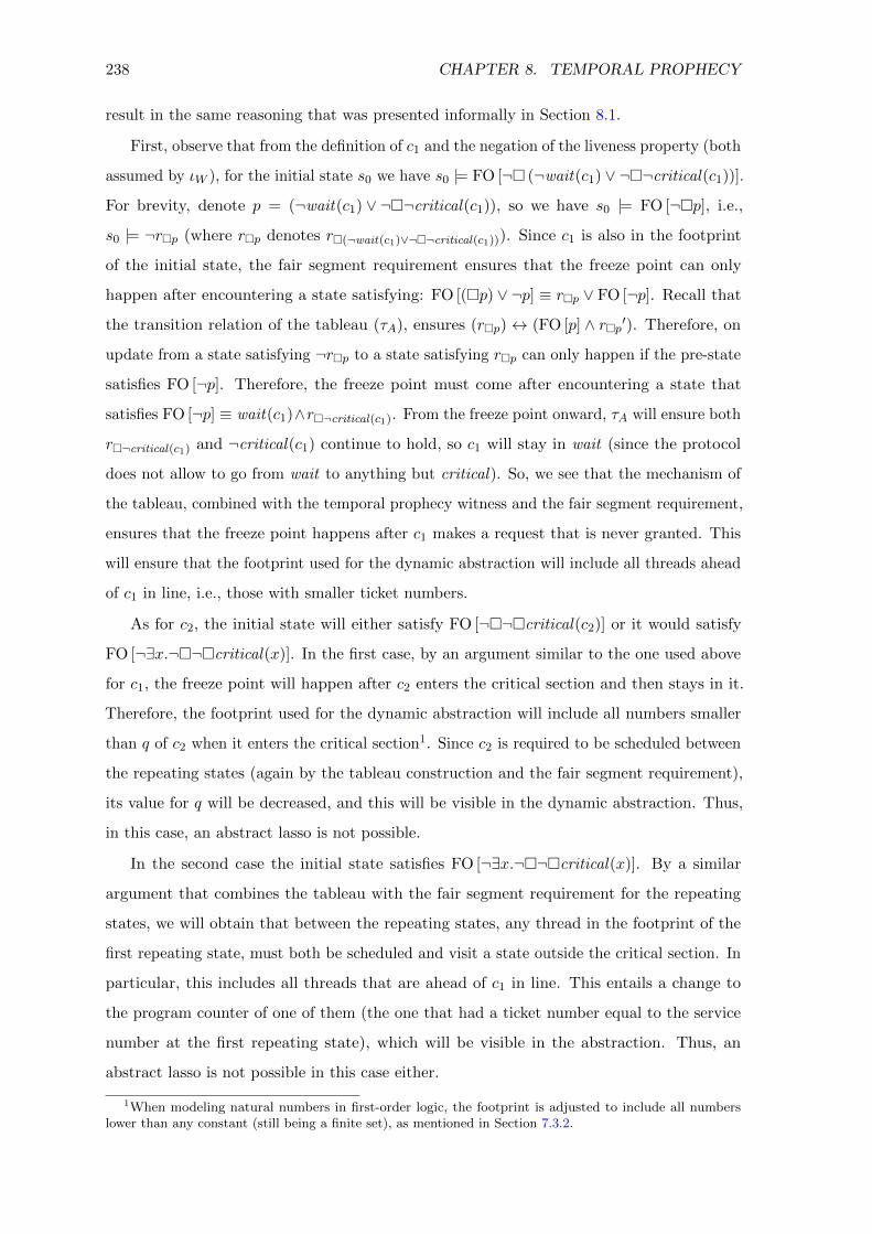
238 CHAPTER 8. TEMPORAL PROPHECY
result in the same reasoning that was presented informally in Section 8.1.
First, observe that from the definition of c1 and the negation of the liveness property (both
assumed by ιW ), for the initial state s0 we have s0 |= FO [¬� (¬wait(c1) ∨ ¬�¬critical(c1))].
For brevity, denote p = (¬wait(c1) ∨ ¬�¬critical(c1)), so we have s0 |= FO [¬�p], i.e.,
s0 |= ¬r�p (where r�p denotes r�(¬wait(c1)∨¬�¬critical(c1))). Since c1 is also in the footprint
of the initial state, the fair segment requirement ensures that the freeze point can only
happen after encountering a state satisfying: FO [(�p) ∨ ¬p] ≡ r�p ∨ FO [¬p]. Recall that
the transition relation of the tableau (τA), ensures (r�p) ↔ (FO [p] ∧ r�p′). Therefore, on
update from a state satisfying ¬r�p to a state satisfying r�p can only happen if the pre-state
satisfies FO [¬p]. Therefore, the freeze point must come after encountering a state that
satisfies FO [¬p] ≡ wait(c1)∧r�¬critical(c1). From the freeze point onward, τA will ensure both
r�¬critical(c1) and ¬critical(c1) continue to hold, so c1 will stay in wait (since the protocol
does not allow to go from wait to anything but critical). So, we see that the mechanism of
the tableau, combined with the temporal prophecy witness and the fair segment requirement,
ensures that the freeze point happens after c1 makes a request that is never granted. This
will ensure that the footprint used for the dynamic abstraction will include all threads ahead
of c1 in line, i.e., those with smaller ticket numbers.
As for c2, the initial state will either satisfy FO [¬�¬�critical(c2)] or it would satisfy
FO [¬∃x.¬�¬�critical(x)]. In the first case, by an argument similar to the one used above
for c1, the freeze point will happen after c2 enters the critical section and then stays in it.
Therefore, the footprint used for the dynamic abstraction will include all numbers smaller
than q of c2 when it enters the critical section1. Since c2 is required to be scheduled between
the repeating states (again by the tableau construction and the fair segment requirement),
its value for q will be decreased, and this will be visible in the dynamic abstraction. Thus,
in this case, an abstract lasso is not possible.
In the second case the initial state satisfies FO [¬∃x.¬�¬�critical(x)]. By a similar
argument that combines the tableau with the fair segment requirement for the repeating
states, we will obtain that between the repeating states, any thread in the footprint of the
first repeating state, must both be scheduled and visit a state outside the critical section. In
particular, this includes all threads that are ahead of c1 in line. This entails a change to
the program counter of one of them (the one that had a ticket number equal to the service
number at the first repeating state), which will be visible in the abstraction. Thus, an
abstract lasso is not possible in this case either.
1When modeling natural numbers in first-order logic, the footprint is adjusted to include all numberslower than any constant (still being a finite set), as mentioned in Section 7.3.2.

8.4. CLOSURE UNDER FIRST-ORDER REASONING 239
8.4 Closure Under First-Order Reasoning
The reduction from temporal verification to safety verification enhanced by temporal prophecy,
as summarized in Theorem 8.10, still involves an abstraction, and incurs a loss of precision.
That is, for some systems and properties, liveness holds but the safety of the resulting
system does not hold, no matter what temporal prophecy is used. (This is unavoidable for a
reduction from arbitrary FO-LTL properties to safety properties, as mentioned in Chapter 7.)
However, in this section, we show that the set of instances for which the reduction can be
made precise (via temporal prophecy) is closed under first-order reasoning. This is unlike the
reduction of Chapter 7. It shows that the use of temporal prophecy results in a particular
kind of robustness.
We consider a proof system in which the reduction of Section 8.3, i.e., with temporal
prophecy, is performed and the resulting safety property is checked by an oracle. That is,
for a transition system T and a temporal property ϕ (a closed FO-LTL formula), we write
T ` ϕ if there exist finite sets of FO-LTL formulas A and B satisfying the conditions of
Theorem 8.10, such that the resulting transition system is safe, i.e., TW does not contain an
abstract lasso.
We now show that the relation ` satisfies a powerful closure property.
Theorem 8.11 (Closure under first-order reasoning). Let T be a transition system, and
ψ,ϕ1, . . . , ϕn be closed FO-LTL formulas, such that FO [ϕ1 ∧ . . . ∧ ϕn] |= FO [ψ]. If T ` ϕifor all 1 ≤ i ≤ n, then T ` ψ.
The condition that FO [ϕ1 ∧ . . . ∧ ϕn] |= FO [ψ] means that ϕ1 ∧ . . . ∧ ϕn entails ψ when
using only first-order reasoning, and treating temporal operators as uninterpreted. The
theorem states that provability using the liveness-to-safety reduction with temporal prophecy
and prophecy witnesses is closed under such reasoning. Two special cases of Theorem 8.11
given by the following corollaries:
Corollary 8.12 (Modus Ponens). If T is a transition system and ϕ and ψ are closed
FO-LTL formulas such that T ` ϕ and T ` ϕ→ ψ, then T ` ψ.
Corollary 8.13 (Cut). If T is a transition system and ϕ and ψ are closed FO-LTL formulas
such that T ` ϕ→ ψ and T ` ¬ϕ→ ψ, then T ` ψ.
Proof of Theorem 8.11. In the proof we use the notation TW (T, ϕ,A,B) to denote the
transition system constructed for T and ϕ when using A,B as temporal prophecy formulas.
Likewise, we refer to the vocabulary, initial states and transition relation formulas of

240 CHAPTER 8. TEMPORAL PROPHECY
the transition system as ΣW (T, ϕ,A,B), ιW (T, ϕ,A,B), and τW (T, ϕ,A,B), respectively.
Let (A1, B1), . . . , (An, Bn) be such that TW (T, ϕi, Ai, Bi) has no abstract lasso, for every
1 ≤ i ≤ n. Now, let A =⋃ni=1Ai and B =
⋃ni=1Bi. We show that TW (T, ψ,A,B) has no
abstract lasso. Assume to the contrary that s0, . . . , si, . . . , sj , . . . , sk, . . . , sn is an abstract
lasso for TW (T, ψ,A,B). Since s0 |= ιW (T, ψ,A,B), we know that s0 |= ¬FO [ψ], and since
FO [ϕ1 ∧ . . . ∧ ϕn] |= FO [ψ], there must be some 1 ≤ ` ≤ n s.t. s0 |= ¬FO [ϕ`]. Denote Σ′ =
ΣW (T, ϕ`, A`, B`). Now, s0|Σ′ , . . . , si|Σ′ , . . . , sj |Σ′ , . . . , sk|Σ′ , . . . , sn|Σ′ is an abstract lasso of
TW (T, ϕ`, A`, B`), which is a contradiction. To see that, we first simplify the notation and
denote sm|Σ′ by sm. Let f(s0, . . . , si) denote the footprint of the trace s0, . . . , si, and similarly
for f(s0, . . . , si). The footprint f(s0, . . . , si) contains more elements than the footprint
f(s0, . . . , si), since ΣW (T, ψ,A,B) ⊇ ΣW (T, ϕ`, A`, B`). Therefore, given that sj |f(s0,...,si) =
sk|f(s0,...,si), we have that sj |f(s0,...,si) = sk|f(s0,...,si) as well. Moreover, the fairness constraints
in TW (T, ϕ`, A`, B`), determined by A`, are a subset of those in TW (T, ψ,A,B)), determined
by A, so the segments [0, i] and [j, k] are also fair in TW (T, ϕ`, A`, B`).
The proof of Theorem 8.11 sheds more light on the power of using temporal prophecy
formulas that are not subformulas of the temporal property to prove. In particular, the
theorem does not hold if A is restricted to subformulas of the temporal proof goal.
8.5 Implementation & Evaluation
We have implemented the temporal verification approach described in this chapter and
integrated it into the Ivy deductive verification system. We have also evaluated the benefit
of temporal prophecy on several challenging examples. Below we report on the scheme
of integrating the liveness-to-safety reduction with temporal prophecy into Ivy, report on
protocols we verified to evaluate it, and compare it to the nesting structure of Chapter 7.
8.5.1 Integration in Ivy
Our implementation in Ivy allows the user to model the transition system in the Ivy language
(which internally translates into a first-order transition system), and express temporal
properties directly in FO-LTL. In our implementation, the safety property that results from
the liveness-to-safety reduction is proven by a suitable inductive invariant, provided by the
user. Ivy internally constructs TW , and composes it with a suitable monitor for the safety
property, i.e., the absence of abstract lasso’s in TW , as described in Theorem 8.10. The
user then provides an inductive invariant for TW composed with the monitor. As explained

8.5. IMPLEMENTATION & EVALUATION 241
in Section 7.3.2, the monitor keeps track of the footprint and the fairness constraints, and
non-deterministically selects the freeze point and repeated states of the abstract lasso. The
monitor keeps a shadow copy of the “saved state”, which is the first of the two repeated
states. These are maintained via designated relation symbols (in addition to ΣW ). The
user’s inductive invariant must then prove that it is impossible for the monitor to detect an
abstract lasso.
Mining temporal prophecy from the inductive invariant As presented in previous
sections, our liveness-to-safety reduction is parameterized by sets of formulas A and B.
In the implementation, these sets are implicit, and are extracted automatically from the
inductive invariant provided by the user. The inductive invariant provided by the user
contains temporal formulas, and also prophecy witness constants, where every temporal
formula �ϕ is a shorthand, and is internally rewritten to, r�ϕ. The set A to be used in
the construction is defined by all the temporal subformulas that appear in the inductive
invariant (and all their subformulas), and the set B is defined according to the prophecy
witness constants that are used in the inductive invariant.
In addition, the user’s invariant may refer to the satisfaction of each fairness constraint
FO [�ϕ ∨ ¬ϕ] for �ϕ ∈ A, both before the freeze point and between the repeated states, via
a convenient syntax provided by Ivy and illustrated in Section 8.5.2.1.
Interacting with Ivy If the user provides an inductive invariant that is not inductive,
Ivy presents a graphical counterexample to induction. This guides the user to adjust the
inductive invariant, which may also lead to new formulas being added to A or B, if the
user adds new temporal formulas or prophecy witnesses to the inductive invariant. In this
process, the user’s mental image is of a liveness-to-safety reduction where A and B include
all (countably many) FO-LTL formulas over the system’s vocabulary, so the user is free
to use any temporal formula, or prophecy witness for any formula. However, since the
user’s inductive invariant is a finite formula, the liveness-to-safety reduction needs only to
be applied to finite A and B, and the infinite A and B are just a mental model.
8.5.2 Examples
We have used our implementation to prove liveness for several challenging examples, sum-
marized in Figure 8.14. We focused here on examples that were beyond reach for the
liveness-to-safety reduction of Chapter 7, unless a nesting structure is used. Our experience
shows that with temporal prophecy, the invariants are simpler than with a nesting structure
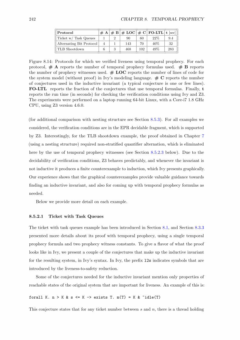
242 CHAPTER 8. TEMPORAL PROPHECY
Protocol # A # B # LOC # C FO-LTL t [sec]
Ticket w/ Task Queues 1 2 90 60 22% 9.4
Alternating Bit Protocol 4 1 143 70 40% 32
TLB Shootdown 6 3 468 102 49% 283
Figure 8.14: Protocols for which we verified liveness using temporal prophecy. For eachprotocol, # A reports the number of temporal prophecy formulas used. # B reportsthe number of prophecy witnesses used. # LOC reports the number of lines of code forthe system model (without proof) in Ivy’s modeling language. # C reports the numberof conjectures used in the inductive invariant (a typical conjecture is one or few lines).FO-LTL reports the fraction of the conjectures that use temporal formulas. Finally, treports the run time (in seconds) for checking the verification conditions using Ivy and Z3.The experiments were performed on a laptop running 64-bit Linux, with a Core-i7 1.8 GHzCPU, using Z3 version 4.6.0.
(for additional comparison with nesting structure see Section 8.5.3). For all examples we
considered, the verification conditions are in the EPR decidable fragment, which is supported
by Z3. Interestingly, for the TLB shootdown example, the proof obtained in Chapter 7
(using a nesting structure) required non-stratified quantifier alternation, which is eliminated
here by the use of temporal prophecy witnesses (see Section 8.5.2.3 below). Due to the
decidability of verification conditions, Z3 behaves predictably, and whenever the invariant is
not inductive it produces a finite counterexample to induction, which Ivy presents graphically.
Our experience shows that the graphical counterexamples provide valuable guidance towards
finding an inductive invariant, and also for coming up with temporal prophecy formulas as
needed.
Below we provide more detail on each example.
8.5.2.1 Ticket with Task Queues
The ticket with task queues example has been introduced in Section 8.1, and Section 8.3.3
presented more details about its proof with temporal prophecy, using a single temporal
prophecy formula and two prophecy witness constants. To give a flavor of what the proof
looks like in Ivy, we present a couple of the conjectures that make up the inductive invariant
for the resulting system, in Ivy’s syntax. In Ivy, the prefix l2s indicates symbols that are
introduced by the liveness-to-safety reduction.
Some of the conjectures needed for the inductive invariant mention only properties of
reachable states of the original system that are important for liveness. An example of this is:
forall K. n > K & s <= K -> exists T. m(T) = K & ~idle(T)
This conjecture states that for any ticket number between s and n, there is a thread holding

8.5. IMPLEMENTATION & EVALUATION 243
that ticket that is also not in the idle state (see Figure 8.1).
Some conjectures are needed to state that the footprint used in the dynamic abstraction
contains enough elements. An example of such a conjecture is:
l2s_frozen & (globally critical(c2)) -> forall N. N <= q(c2) -> l2s_a(N)
This conjecture states that after the freeze point (indicated by the special symbol l2s frozen),
if the prophecy witness c2 (which is the prophecy witness defined for ♦�critical(x)) is globally
in the critical section, then the finite domain of the frozen abstraction (stored in the unary
relation l2s a) contains all numbers up to q(c2).
Other conjectures are needed to show that the current state is different from the saved
state. One example is:
l2s_saved & (globally critical(c2)) & ~($l2s_w X. scheduled(X))(c2) ->
q(c2) ~= ($l2s_s X. q(X))(c2)
The special operator $l2s w lets the user query whether a fairness constraint has been
encountered, and $l2s s exposes to the user the saved state (both syntactically λ-like
binders). This conjecture states that after we saved a shadow state (indicated by l2s saved),
if the prophecy witness c2 is globally in the critical section, and if we have encountered
the fairness constraints associated with scheduled(x) ∨�¬scheduled(x) instantiated for c2
(which can only happen after c2 has been scheduled), then the current value c2 has for q is
different from the same value in the shadow state.
8.5.2.2 Alternating Bit Protocol
The alternating bit protocol (also presented in Section 7.4.1) is a classic communication algo-
rithm for transition of messages using lossy first-in-first-out (FIFO) channels. The protocol
uses two channels: a data channel from the sender to the receiver, and an acknowledgment
channel from the receiver to the sender. The sender and the receiver each have a state bit,
and messages include a bit that functions as a “sequence number”. We assume that the
sender has an (infinite) array of values to send, which is filled by some independent process.
The liveness property we wish to prove is that every value entered into the sender array is
eventually received by the receiver.
The protocol is live under fair scheduling assumptions, as well as standard fairness
constraints for the channels: if messages are infinitely often sent, then messages are infinitely
often received. This makes the structure of the temporal property more involved. Formally,

244 CHAPTER 8. TEMPORAL PROPHECY
the liveness property we prove is:
(�♦sender scheduled) ∧ (�♦receiver scheduled)∧
((�♦data sent)→ (�♦data received)) ∧ ((�♦ack sent)→ (�♦ack received)) →
∀x.�(sender array(x) 6= ⊥ → ♦receiver array(x) 6= ⊥))
As explained in Section 7.4.2, this property cannot be proven without temporal prophecy or
a nesting structure. However, it can be proven using 4 temporal prophecy formulas:
{♦� (sender bit = s ∧ receiver bit = r) | s, r ∈ {0, 1}}
Intuitively, these formulas make a distinction between traces in which the sender and receiver
bits eventually become fixed, and traces in which they change infinitely often.
8.5.2.3 TLB Shootdown
The TLB shootdown algorithm [29], also considered in Section 7.6.1, is used (e.g., in the
Mach operating system) to maintain consistency of Translation Look-aside Buffers (TLB)
across processors. When some processor (dubbed the initiator) changes the page table, it
interrupts all other processors currently using the page table (dubbed the responders) and
waits for them to receive the interrupt before making changes.
The liveness property we prove is that no processor can become stuck either as an initiator
or as a responder (formally, it will respond or initiate infinitely often). This liveness depends
on fair scheduling assumptions, as well as strong fairness assumptions for the page table
locks used by the protocol.
We use one witness for the process that does not satisfy the liveness property. Another
witness is used for a pagemap that is never unlocked, if this exists. A third witness is used
for a process that possibly gets stuck while holding the lock blocking the first process.
We use six prophecy formulas to case split on when some process may get stuck. Two of
them are used for the two loops in the initiator to distinguish the cases whether the process
that hogs the lock gets stuck there. They are of the form ♦�pc(c2) ∈ {i3, . . . , i8}. Two are
used for the two lock instructions to indicate that the first process gets stuck: ♦�pc(c1) = i2.
And two are used for the second and third witness to indicate whether such a witness exists,
e.g., ♦�plock(c3). Compared to the proof of Chapter 7, our proof is simpler due to the
temporal prophecy, and avoids non-stratified quantifier alternation, resulting in decidable
verification conditions.

8.6. RELATED WORK FOR CHAPTER 8 245
8.5.3 Comparison With Chapter 7
Comparing Figure 8.14 and Figure 7.23, we see that here we generally use more conjectures.
The reason for this is that in the evaluation described in Section 7.6, temporal monitors were
constructed manually, and contained some shortcuts. In contrast, the tableau construction
(Section 8.2), which is made automatic in this chapter (and implemented in Ivy), results in
systems that require slightly more verbose invariants. To illustrate this on the ticket protocol,
note that FO [∀x.�♦scheduled(x)] must be included in the inductive invariant to assert that
it keeps holding. In contrast, in the evaluation of Section 7.6, scheduled(x) was taken as
an apriori fairness constraint, which is a manual optimization of the tableau construction.
For the Alternating Bit Protocol, some conjectures related to fairness constraints repeat 4
times, for combinations of sender and receiver bit values. Similarly, in the TLB Shootdown
example, further conjectures are needed to track properties of the prophecy formulas and
the witness constants.
Comparing temporal prophecy to the nesting structure introduced in Section 7.4, we note
that a nesting structure must be defined by the user (via first-order formulas), and has the
effect of splitting the transition system into levels (analogous to nested loops) and proving
each level separately. Temporal prophecy in contrast is more general, and in particular, any
proof that is possible with a nesting structure, is also possible with temporal prophecy (by
adding a temporal prophecy formula ♦�δ for every nesting level, defined by δ). However,
our experience is that coming up with temporal prophecy is usually easier and more natural
than coming up with a nesting structure. Moreover, the nesting structure does not admit
cut elimination or closure under first-order reasoning, and is therefore less robust.
8.6 Related Work for Chapter 8
Prophecy variables were first introduced in [3], in the context of refinement mappings. There,
prophecy variables are required to range over a finite domain to ensure soundness. Our
notion of prophecy via first-order temporal formulas and witness constants does not meet
this criterion, but is still sound as assured by Theorem 8.10. In [118], LTL formulas are used
to define prophecy variables in a way that is similar to ours, but only to show refinement
between finite-state processes. We use temporal prophecy defined by FO-LTL formulas in
the context of infinite-state systems. Furthermore, we consider a liveness-to-safety reduction
(rather than refinement mappings), which can be seen as a proof system for FO-LTL.
One effect of prophecy is to split cases in the proof on some aspect of the future. This

246 CHAPTER 8. TEMPORAL PROPHECY
very general idea occurs in various approaches to liveness, particularly in the large body of
work on lexicographic or disjunctive rankings for termination [17, 36, 48, 51, 52, 55, 81, 89,
95, 98, 128, 146, 200, 201, 226–228, 230]. In the work of [97], the partitioning of the space of
potentially infinite executions is based on the a priori decomposition of regular expressions
for iterated loop segments. Often the partitioning here amounts to a split according to a
fairness condition (“command a is taken infinitely often or it is not”). The partitioning is
constructed dynamically (and represented explicitly through a union of Buchi automata)
in [101] (for termination), in [64] (for liveness), and in [73] (for liveness of parameterized
systems). None of these works uses a temporal tableau construction to partition the space
of futures, however.
Here, we use prophecy to, in effect, partially determinize a system by making non-
deterministic choices earlier in an execution. This same effect was used for a different purpose
in refining an abstraction from LTL to ACTL [50] and checking CTL* properties [53]. The
prophecy in this case relates only to the next transition and is not expressed temporally. The
method of “temporal case splitting” in [170] can also be seen as a way to introduce prophecy
variables to increase the precision of an abstraction, though in that case the reduction was to
finite-state liveness, not infinite-state safety. Moreover, it only introduces temporal witnesses.
We have considered only proof methods that reduce liveness to safety (which includes
the classical ranking approach for while loops). There are approaches, however, which do
not reduce liveness to safety. For example, the approaches in [8, 55, 229] are essentially
forms of widening in a CTL-style backwards fixpoint iteration. It is not clear to what extent
temporal prophecy might be useful in increasing the precision of such abstractions, but it
may be an interesting topic for future research.


Chapter 9
Conclusion
The central theme explored in this thesis is using first-order logic, and the EPR decidable
fragment, for deductive verification. As we have seen, this seemingly weak and inexpressive
fragment can be made surprisingly powerful, by using appropriate encodings and abstractions,
and by utilizing a technique for elimination of quantifier alternation cycles when they arise.
We have also seen a technique for proving liveness and temporal properties that fits well
with the scheme of first-order logic based verification, and does not require ranking functions
nor reasoning about arithmetic.
From a practical perspective, this thesis provides a step towards increasing the pro-
ductivity and practicality of deductive verification using automated theorem provers. The
increase in productivity is obtained by using the automated solvers only on a decidable
logical fragment, which leads to greater solver stability, and as a result to a more productive
and enjoyable verification process. To obtain this, one must pay the cost of engineering
the verification such that VCs are always in the decidable fragment. The initial experience
presented in this thesis suggests that this is possible in many interesting cases, and that the
effort is worthwhile.
The techniques developed in this thesis have been implemented in the Ivy deductive
verification system, and successfully applied to verify several protocols, some formally verified
for the first time. It is encouraging to note that EPR was powerful enough to verify protocols
from the Paxos family including Stoppable Paxos, as well as other protocols such as the
Chord protocol and the TLB Shootdown protocol. These protocols are quite challenging to
verify, and the verification obtained in this thesis required significantly less effort compared
to state-of-the-art techniques.
Aside from this thesis, the author has used Ivy in a verification workshop course in Tel
Aviv University. Twenty undergraduate students participated in the workshop, and each
249

250 CHAPTER 9. CONCLUSION
team of 2-3 students verified safety of a classic mutual exclusion protocol. The workshop was
encouraging as all the students were able to use Ivy’s modeling language to model protocols as
transition systems in first-order logic, and were successful in finding comprehensible inductive
invariants. While working with Ivy, the students greatly benefited from the fact that Z3 is a
practically stable decision procedure for EPR. The finite counterexamples produced by Z3
and displayed by Ivy were key in enabling the students to find correct inductive invariants.
In the setting of using first-order logic for deductive verification, and with the VCs set in
a decidable logic, this thesis also explored the question of invariant inference. We have seen
several decidability and undecidability results for the invariant inference problem. While
these results were developed and presented primarily in a theoretical mindset, the author
hopes that some of the ideas presented can also be useful in designing practical heuristics for
automated or semi-automated invariant inference. This thesis also presented a technique for
finding universally quantified inductive invariants in a cooperative process between the user
and well-defined decidable automated queries. While the technique presented here targets
universally quantified invariants, the idea of a systematic interactive process for finding
inductive invariants is general, and can hopefully be extended to other classes of inductive
invariants.
For liveness proofs, we have seen a powerful proof technique that is based on transforming
liveness verification to safety verification, by exploiting the representation of states as
first-order structures. The transformation involves an abstraction, and we have seen two
mechanisms for increasing the precision of the abstraction: a nesting structure that allows
to split the proof into nested levels, analogous to nested loops; and the more powerful
mechanism of temporal prophecy, which also leads to a cut elimination theorem for the proof
method. Temporal prophecy also facilitates verification using EPR, as it allows to eliminate
some quantifiers from inductive invariants by replacing them with a special kind of Skolem
constants.
While the liveness verification techniques developed in this thesis were presented in the
context of verification based on first-order logic, some of the ideas behind them are actually
general, and can hopefully be useful in other contexts. The idea of dynamic abstraction,
as a technique for proving liveness and temporal properties, does not depend on the use of
first-order logic; and the parameterized formulation of dynamic abstraction developed here
may be instantiated in other contexts. The idea of temporal prophecy is also general, and
using prophecy variables defined by temporal formulas may also benefit other liveness and
termination proofs techniques.

251
Finally, as this thesis developed several techniques for reducing safety and liveness
verification of complex protocols to decidable EPR satisfiability queries, an interesting
question that remains open is the following: what is it about these protocols that makes it
possible to reduce their verification to EPR queries? The techniques developed in this thesis
were successfully applied to a variety of protocols (e.g., several Paxos variants, Chord, TLB
Shootdown). Furthermore, the techniques’ structure is also general and influenced mostly by
logical considerations (e.g., handling quantifiers), rather than protocol specific ones. However,
it is clear that the developed techniques are not a complete proof system, and not every
infinite-state system can be verified in EPR; in particular, this would contradict Godel’s
incompleteness theorems [90]. Despite trying, the author has not been able to find any
interesting case of a protocol that provably cannot be verified in EPR. (For an uninteresting
case, construct a system whose safety or liveness depends on the truth of the Godel sentence
of ZFC.) It therefore remains for future research to obtain a better theoretical understanding
of what systems can be proven by EPR.
Another perspective on this issue is that the provability of a system in EPR (i.e., by the
techniques we have seen) exploits and uncovers some simplicity that exists in the system
and its correctness argument. The simplicity exists even though the system is expressed in a
Turing-complete formalism that does not make it apparent. This situation occurs across
most of the field of program analysis and verification: we devise an algorithm or a method
to analyze programs, which is known to be theoretically impossible; yet we expect that the
specific programs encountered in practice will have some simplicity in them that will allow
our method to succeed. (Even for classes in which verification is theoretically decidable, the
theoretical time complexity is very high, yet we expect practical run time to be reasonable.)
The author hopes that in the future, we will have a better theoretical understanding of this
simplicity, which underlies our expectation that program analysis and verification methods
would succeed in spite of the theoretical intractability of the problems they aim to solve.

Bibliography
[1] Aharon Abadi, Alexander Rabinovich, and Mooly Sagiv. Decidable fragments of many-
sorted logic. J. Symb. Comput., 45(2):153–172, 2010. doi: 10.1016/j.jsc.2009.03.003.
URL https://doi.org/10.1016/j.jsc.2009.03.003. 15, 35
[2] Martın Abadi. The power of temporal proofs. Theor. Comput. Sci., 65(1):35–
83, 1989. doi: 10.1016/0304-3975(89)90138-2. URL https://doi.org/10.1016/
0304-3975(89)90138-2. 21, 184, 189, 194, 195
[3] Martın Abadi and Leslie Lamport. The existence of refinement mappings. Theor.
Comput. Sci., 82(2):253–284, 1991. doi: 10.1016/0304-3975(91)90224-P. URL https:
//doi.org/10.1016/0304-3975(91)90224-P. 245
[4] Parosh Abdulla and Bengt Jonsson. Verifying programs with unreliable channels.
In Logic in Computer Science, 1993. LICS’93., Proceedings of Eighth Annual IEEE
Symposium on, pages 160–170. IEEE, 1993. 154
[5] Parosh Aziz Abdulla and Bengt Jonsson. Ensuring completeness of symbolic verification
methods for infinite-state systems. Theoretical Computer Science, 256(1):145–167,
2001. 18, 113, 115, 121, 154
[6] Parosh Aziz Abdulla, Karlis Cerans, Bengt Jonsson, and Yih-Kuen Tsay. General
decidability theorems for infinite-state systems. In Logic in Computer Science, 1996.
LICS’96. Proceedings., Eleventh Annual IEEE Symposium on, pages 313–321. IEEE,
1996. 8, 18, 113, 115, 121, 154
[7] Parosh Aziz Abdulla, Karlis Cerans, Bengt Jonsson, and Yih-Kuen Tsay. Algorithmic
analysis of programs with well quasi-ordered domains. Information and Computation,
160(1):109–127, 2000. doi: 10.1006/inco.1999.2843. URL http://dx.doi.org/10.
1006/inco.1999.2843. 18, 113, 115, 121, 154, 182
253

254 BIBLIOGRAPHY
[8] Parosh Aziz Abdulla, Bengt Jonsson, Ahmed Rezine, and Mayank Saksena. Proving
liveness by backwards reachability. In CONCUR, volume 4137 of Lecture Notes in
Computer Science, pages 95–109. Springer, 2006. 218, 224, 246
[9] Parosh Aziz Abdulla, Giorgio Delzanno, Noomene Ben Henda, and Ahmed Rezine.
Regular model checking without transducers (on efficient verification of parameterized
systems). In Tools and Algorithms for the Construction and Analysis of Systems, pages
721–736. Springer, 2007. 18, 113, 121, 154
[10] Parosh Aziz Abdulla, Ahmed Bouajjani, Jonathan Cederberg, Frederic Haziza, and
Ahmed Rezine. Monotonic abstraction for programs with dynamic memory heaps. In
CAV’08, pages 341–354, 2008. 155
[11] Parosh Aziz Abdulla, Jonathan Cederberg, and Tomas Vojnar. Monotonic abstraction
for programs with multiply-linked structures. Int. J. Found. Comput. Sci., 24(2):
187–210, 2013. 155
[12] Ittai Abraham, Guy Gueta, Dahlia Malkhi, Lorenzo Alvisi, Ramakrishna Kotla, and
Jean-Philippe Martin. Revisiting fast practical byzantine fault tolerance. CoRR,
abs/1712.01367, 2017. URL http://arxiv.org/abs/1712.01367. 11
[13] Ittai Abraham, Guy Gueta, Dahlia Malkhi, and Jean-Philippe Martin. Revisiting fast
practical byzantine fault tolerance: Thelma, velma, and zelma. CoRR, abs/1801.10022,
2018. URL http://arxiv.org/abs/1801.10022. 11
[14] Francesco Alberti, Silvio Ghilardi, and Elena Pagani. Counting Constraints in Flat
Array Fragments. In Automated Reasoning, pages 65–81. Springer, Cham, 2016. 73,
107
[15] Bowen Alpern and Fred B. Schneider. Defining liveness. Information processing letters,
21(4):181–185, 1985. 9, 36
[16] Hagit Attiya and Jennifer Welch. Distributed Computing: Fundamentals, Simulations
and Advanced Topics. John Wiley & Sons, Inc., USA, 2004. ISBN 0471453242. 9
[17] Domagoj Babic, Alan J. Hu, Zvonimir Rakamaric, and Byron Cook. Proving termina-
tion by divergence. In SEFM, pages 93–102, 2007. 246
[18] Kyungmin Bae and Jose Meseguer. State/event-based ltl model checking under
parametric generalized fairness. In Ganesh Gopalakrishnan and Shaz Qadeer, editors,

BIBLIOGRAPHY 255
Computer Aided Verification: 23rd International Conference, CAV 2011, Snowbird, UT,
USA, July 14-20, 2011. Proceedings, pages 132–148, Berlin, Heidelberg, 2011. Springer
Berlin Heidelberg. ISBN 978-3-642-22110-1. doi: 10.1007/978-3-642-22110-1 11. URL
https://doi.org/10.1007/978-3-642-22110-1_11. 223
[19] Kyungmin Bae and Jose Meseguer. Infinite-state model checking of LTLR formulas
using narrowing. In Rewriting Logic and Its Applications - 10th International Workshop,
WRLA 2014, Held as a Satellite Event of ETAPS, Grenoble, France, April 5-6, 2014,
Revised Selected Papers, pages 113–129, 2014. doi: 10.1007/978-3-319-12904-4 6. URL
https://doi.org/10.1007/978-3-319-12904-4_6. 223
[20] Kyungmin Bae and Jose Meseguer. Model checking linear temporal logic of rewriting
formulas under localized fairness. Science of Computer Programming, 99(Supplement
C):193 – 234, 2015. ISSN 0167-6423. doi: https://doi.org/10.1016/j.scico.2014.02.006.
URL http://www.sciencedirect.com/science/article/pii/S0167642314000471.
Selected Papers from the Ninth International Workshop on Rewriting Logic and its
Applications (WRLA 2012). 223
[21] Kshitij Bansal, Andrew Reynolds, Clark W. Barrett, and Cesare Tinelli. A new decision
procedure for finite sets and cardinality constraints in SMT. In Nicola Olivetti and
Ashish Tiwari, editors, Automated Reasoning - 8th International Joint Conference,
IJCAR 2016, Coimbra, Portugal, June 27 - July 2, 2016, Proceedings, volume 9706
of Lecture Notes in Computer Science, pages 82–98. Springer, 2016. ISBN 978-3-
319-40228-4. doi: 10.1007/978-3-319-40229-1\ 7. URL https://doi.org/10.1007/
978-3-319-40229-1_7. 73
[22] Clark Barrett, Christopher L. Conway, Morgan Deters, Liana Hadarean, Dejan Jo-
vanovi’c, Tim King, Andrew Reynolds, and Cesare Tinelli. CVC4. In Ganesh
Gopalakrishnan and Shaz Qadeer, editors, Proceedings of the 23rd International
Conference on Computer Aided Verification (CAV ’11), volume 6806 of Lecture
Notes in Computer Science, pages 171–177. Springer, July 2011. URL http:
//www.cs.stanford.edu/~barrett/pubs/BCD+11.pdf. Snowbird, Utah. 3
[23] Clark W. Barrett, Roberto Sebastiani, Sanjit A. Seshia, and Cesare Tinelli. Satisfiability
modulo theories. In Armin Biere, Marijn Heule, Hans van Maaren, and Toby Walsh,
editors, Handbook of Satisfiability, volume 185 of Frontiers in Artificial Intelligence and
Applications, pages 825–885. IOS Press, 2009. ISBN 978-1-58603-929-5. doi: 10.3233/

256 BIBLIOGRAPHY
978-1-58603-929-5-825. URL https://doi.org/10.3233/978-1-58603-929-5-825.
3
[24] Amir M. Ben-Amram. General size-change termination and lexicographic descent.
In The Essence of Computation, volume 2566 of Lecture Notes in Computer Science,
pages 3–17. Springer, 2002. 223
[25] Josh Berdine, Cristiano Calcagno, and Peter W. O’Hearn. A decidable fragment of
separation logic. In FSTTCS 2004: Foundations of Software Technology and Theoretical
Computer Science, 24th International Conference, Chennai, India, December 16-18,
2004, Proceedings, pages 97–109, 2004. doi: 10.1007/978-3-540-30538-5\ 9. URL
https://doi.org/10.1007/978-3-540-30538-5_9. 5
[26] Yves Bertot and Pierre Casteran. Interactive Theorem Proving and Program Devel-
opment - Coq’Art: The Calculus of Inductive Constructions. Texts in Theoretical
Computer Science. An EATCS Series. Springer, 2004. ISBN 978-3-642-05880-6. doi: 10.
1007/978-3-662-07964-5. URL http://dx.doi.org/10.1007/978-3-662-07964-5.
2, 108, 158, 182
[27] Armin Biere, Cyrille Artho, and Viktor Schuppan. Liveness checking as safety checking.
Electr. Notes Theor. Comput. Sci., 66(2):160–177, 2002. 21, 186, 192, 222, 226
[28] Ken Birman. A history of the virtual synchrony replication model. In Replication:
Theory and Practice, pages 91–120, 2010. doi: 10.1007/978-3-642-11294-2 6. URL
https://doi.org/10.1007/978-3-642-11294-2_6. 104, 302
[29] D. L. Black, R. F. Rashid, D. B. Golub, and C. R. Hill. Translation lookaside buffer
consistency: A software approach. In Proceedings of the Third International Conference
on Architectural Support for Programming Languages and Operating Systems, ASPLOS
III, pages 113–122, New York, NY, USA, 1989. ACM. ISBN 0-89791-300-0. doi:
10.1145/70082.68193. URL http://doi.acm.org/10.1145/70082.68193. 23, 218,
244
[30] Roderick Bloem, Swen Jacobs, Ayrat Khalimov, Igor Konnov, Sasha Rubin, Hel-
mut Veith, and Josef Widder. Decidability of Parameterized Verification. Synthesis
Lectures on Distributed Computing Theory. Morgan & Claypool Publishers, 2015.
doi: 10.2200/S00658ED1V01Y201508DCT013. URL http://dx.doi.org/10.2200/
S00658ED1V01Y201508DCT013. 107, 224

BIBLIOGRAPHY 257
[31] Ahmed Bouajjani, Bengt Jonsson, Marcus Nilsson, and Tayssir Touili. Regular model
checking. In CAV, volume 1855 of Lecture Notes in Computer Science, pages 403–418.
Springer, 2000. 224
[32] Ahmed Bouajjani, Marius Bozga, Peter Habermehl, Radu Iosif, Pierre Moro, and
Tomas Vojnar. Programs with lists are counter automata. Formal Methods in System
Design, 38(2):158–192, 2011. 117, 155
[33] Ana Bove, Peter Dybjer, and Ulf Norell. A brief overview of agda - A functional
language with dependent types. In Stefan Berghofer, Tobias Nipkow, Christian
Urban, and Makarius Wenzel, editors, Theorem Proving in Higher Order Logics,
22nd International Conference, TPHOLs 2009, Munich, Germany, August 17-20,
2009. Proceedings, volume 5674 of Lecture Notes in Computer Science, pages 73–78.
Springer, 2009. ISBN 978-3-642-03358-2. doi: 10.1007/978-3-642-03359-9\ 6. URL
https://doi.org/10.1007/978-3-642-03359-9_6. 2
[34] Aaron R. Bradley. Sat-based model checking without unrolling. In Ranjit Jhala and
David A. Schmidt, editors, Verification, Model Checking, and Abstract Interpretation
- 12th International Conference, VMCAI 2011, Austin, TX, USA, January 23-25,
2011. Proceedings, volume 6538 of Lecture Notes in Computer Science, pages 70–87.
Springer, 2011. ISBN 978-3-642-18274-7. doi: 10.1007/978-3-642-18275-4\ 7. URL
https://doi.org/10.1007/978-3-642-18275-4_7. 18, 113, 155, 182
[35] Aaron R. Bradley, Zohar Manna, and Henny B. Sipma. What’s decidable about
arrays? In Verification, Model Checking, and Abstract Interpretation, 7th International
Conference, VMCAI 2006, Charleston, SC, USA, January 8-10, 2006, Proceedings,
pages 427–442, 2006. doi: 10.1007/11609773 28. URL http://dx.doi.org/10.1007/
11609773_28. 5
[36] Marc Brockschmidt, Byron Cook, and Carsten Fuhs. Better termination proving
through cooperation. In Computer Aided Verification - 25th International Conference,
CAV 2013, Saint Petersburg, Russia, July 13-19, 2013. Proceedings, pages 413–429,
2013. 246
[37] Michael Burrows. The chubby lock service for loosely-coupled distributed systems. In
7th Symposium on Operating Systems Design and Implementation OSDI ’06), November
6-8, Seattle, WA, USA, pages 335–350. USENIX Association, 2006. 10, 24

258 BIBLIOGRAPHY
[38] Alessandro Carioni, Silvio Ghilardi, and Silvio Ranise. Automated termination in
model-checking modulo theories. Int. J. Found. Comput. Sci., 24(2):211–232, 2013.
154
[39] Venkatesan T. Chakaravarthy. New results on the computability and complexity of
points - to analysis. In Conference Record of POPL 2003: The 30th SIGPLAN-SIGACT
Symposium on Principles of Programming Languages, New Orleans, Louisisana, USA,
January 15-17, 2003, pages 115–125, 2003. 155
[40] Saksham Chand, Yanhong A. Liu, and Scott D. Stoller. Formal Verification of Multi-
Paxos for Distributed Consensus. In FM 2016: Formal Methods: 21st International
Symposium, Limassol, Cyprus, November 9-11, 2016, Proceedings 21, pages 119–136.
Springer, 2016. 25, 109
[41] Tushar Deepak Chandra, Robert Griesemer, and Joshua Redstone. Paxos made
live: an engineering perspective. In Indranil Gupta and Roger Wattenhofer, editors,
Proceedings of the Twenty-Sixth Annual ACM Symposium on Principles of Distributed
Computing, PODC 2007, Portland, Oregon, USA, August 12-15, 2007, pages 398–
407. ACM, 2007. ISBN 978-1-59593-616-5. doi: 10.1145/1281100.1281103. URL
http://doi.acm.org/10.1145/1281100.1281103. 24
[42] C.C. Chang and H.J. Keisler. Model Theory. Studies in Logic and the Foundations of
Mathematics. Elsevier Science, 1990. ISBN 9780080880075. 116, 127
[43] Ernest Chang and Rosemary Roberts. An improved algorithm for decentralized
extrema-finding in circular configurations of processes. Communications of the ACM,
22(5):281–283, 1979. 49
[44] Bernadette Charron-Bost and Andr Schiper. The heard-of model: Computing in
distributed systems with benign faults. Distributed Computing, 22(1):49–71, 2009. 107
[45] Kaustuv Chaudhuri, Damien Doligez, Leslie Lamport, and Stephan Merz. The
TLA+Proof System: Building a Heterogeneous Verification Platform. In Proceedings
of the 7th International Colloquium Conference on Theoretical Aspects of Computing,
ICTAC’10, pages 44–44. Springer-Verlag, 2010. ISBN 978-3-642-14807-1. 109
[46] Haogang Chen, Daniel Ziegler, Tej Chajed, Adam Chlipala, M. Frans Kaashoek, and
Nickolai Zeldovich. Using crash hoare logic for certifying the FSCQ file system. In
Proceedings of the 25th Symposium on Operating Systems Principles, SOSP 2015,

BIBLIOGRAPHY 259
Monterey, CA, USA, October 4-7, 2015, pages 18–37, 2015. doi: 10.1145/2815400.
2815402. URL http://doi.acm.org/10.1145/2815400.2815402. 108
[47] Gregory V. Chockler, Idit Keidar, and Roman Vitenberg. Group communication
specifications: a comprehensive study. ACM Comput. Surv., 33(4):427–469, 2001. doi:
10.1145/503112.503113. URL http://doi.acm.org/10.1145/503112.503113. 104,
302
[48] B. Cook, A. Podelski, and A. Rybalchenko. Termination proofs for systems code. In
PLDI, pages 415–426, 2006. 223, 246
[49] B. Cook, A. Gotsman, A. Podelski, A. Rybalchenko, and M. Y. Vardi. Proving that
programs eventually do something good. In Martin Hofmann and Matthias Felleisen,
editors, POPL, pages 265–276, 2007. 223
[50] Byron Cook and Eric Koskinen. Making prophecies with decision predicates. In
Proceedings of the 38th ACM SIGPLAN-SIGACT Symposium on Principles of Pro-
gramming Languages, POPL 2011, Austin, TX, USA, January 26-28, 2011, pages
399–410, 2011. doi: 10.1145/1926385.1926431. URL http://doi.acm.org/10.1145/
1926385.1926431. 246
[51] Byron Cook, Andreas Podelski, and Andrey Rybalchenko. Proving program termination.
Commun. ACM, 54(5):88–98, 2011. 227, 246
[52] Byron Cook, Abigail See, and Florian Zuleger. Ramsey vs. lexicographic termination
proving. In TACAS, pages 47–61, 2013. 246
[53] Byron Cook, Heidy Khlaaf, and Nir Piterman. On automation of ctl* verification for
infinite-state systems. In Computer Aided Verification - 27th International Conference,
CAV 2015, San Francisco, CA, USA, July 18-24, 2015, Proceedings, Part I, pages
13–29, 2015. doi: 10.1007/978-3-319-21690-4 2. URL https://doi.org/10.1007/
978-3-319-21690-4_2. 246
[54] Jonathan Corbet. Ticket spinlocks. https://lwn.net/Articles/267968/, 2008. 189
[55] P. Cousot and R. Cousot. An abstract interpretation framework for termination. In
POPL, pages 245–258, 2012. 224, 246
[56] Patrick Cousot and Radhia Cousot. Abstract interpretation: A unified lattice model
for static analysis of programs by construction or approximation of fixpoints. In

260 BIBLIOGRAPHY
Proceedings of the 4th ACM SIGACT-SIGPLAN Symposium on Principles of Program-
ming Languages, POPL ’77, pages 238–252, New York, NY, USA, 1977. ACM. doi:
10.1145/512950.512973. URL http://doi.acm.org/10.1145/512950.512973. 7, 18,
113, 115
[57] Patrick Cousot and Radhia Cousot. Systematic design of program analysis frameworks.
In Proceedings of the 6th ACM SIGACT-SIGPLAN Symposium on Principles of
Programming Languages, POPL ’79, pages 269–282, New York, NY, USA, 1979. ACM.
doi: 10.1145/567752.567778. URL http://doi.acm.org/10.1145/567752.567778. 7,
18, 113, 115
[58] Patrick Cousot, Radhia Cousot, Jerome Feret, Laurent Mauborgne, Antoine Mine,
David Monniaux, and Xavier Rival. The astree analyzer. In Shmuel Sagiv, edi-
tor, Programming Languages and Systems, 14th European Symposium on Program-
ming,ESOP 2005, Held as Part of the Joint European Conferences on Theory and
Practice of Software, ETAPS 2005, Edinburgh, UK, April 4-8, 2005, Proceedings,
volume 3444 of Lecture Notes in Computer Science, pages 21–30. Springer, 2005. ISBN
3-540-25435-8. doi: 10.1007/978-3-540-31987-0\ 3. URL https://doi.org/10.1007/
978-3-540-31987-0_3. 7
[59] Patrick Cousot, Radhia Cousot, and Francesco Logozzo. A parametric segmentation
functor for fully automatic and scalable array content analysis. In Proceedings of the
38th ACM SIGPLAN-SIGACT Symposium on Principles of Programming Languages,
POPL 2011, Austin, TX, USA, January 26-28, 2011, pages 105–118, 2011. 116
[60] Jakub Daniel, Alessandro Cimatti, Alberto Griggio, Stefano Tonetta, and Sergio Mover.
Infinite-state liveness-to-safety via implicit abstraction and well-founded relations.
In Swarat Chaudhuri and Azadeh Farzan, editors, Computer Aided Verification -
28th International Conference, CAV 2016, Toronto, ON, Canada, July 17-23, 2016,
Proceedings, Part I, volume 9779 of Lecture Notes in Computer Science, pages 271–291.
Springer, 2016. ISBN 978-3-319-41527-7. doi: 10.1007/978-3-319-41528-4 15. URL
https://doi.org/10.1007/978-3-319-41528-4_15. 222
[61] Leonardo de Moura and Nikolaj Bjørner. Z3: An efficient SMT solver. In Tools and
Algorithms for the Construction and Analysis of Systems, 14th International Conference,
TACAS 2008, Held as Part of the Joint European Conferences on Theory and Practice
of Software, ETAPS 2008, Budapest, Hungary, March 29-April 6, 2008. Proceedings,

BIBLIOGRAPHY 261
volume 4963 of Lecture Notes in Computer Science, pages 337–340. Springer, 2008. 3,
105, 158, 177, 216
[62] Leonardo De Moura and Nikolaj Bjørner. Satisfiability modulo theories: Introduction
and applications. Commun. ACM, 54(9):69–77, September 2011. ISSN 0001-0782. doi:
10.1145/1995376.1995394. URL http://doi.acm.org/10.1145/1995376.1995394. 3
[63] Leonardo Mendonca de Moura, Soonho Kong, Jeremy Avigad, Floris van Doorn, and
Jakob von Raumer. The lean theorem prover (system description). In Amy P. Felty
and Aart Middeldorp, editors, Automated Deduction - CADE-25 - 25th International
Conference on Automated Deduction, Berlin, Germany, August 1-7, 2015, Proceedings,
volume 9195 of Lecture Notes in Computer Science, pages 378–388. Springer, 2015.
ISBN 978-3-319-21400-9. doi: 10.1007/978-3-319-21401-6\ 26. URL https://doi.
org/10.1007/978-3-319-21401-6_26. 2
[64] Daniel Dietsch, Matthias Heizmann, Vincent Langenfeld, and Andreas Podelski. Fair-
ness modulo theory: A new approach to LTL software model checking. In CAV, volume
9206 of Lecture Notes in Computer Science, pages 49–66. Springer, 2015. 223, 246
[65] Edsger W. Dijkstra. A short introduction to the art of programming. EWD316,
circulated privately., August 1971. URL http://www.cs.utexas.edu/users/EWD/
ewd03xx/EWD316.PDF. 6
[66] Edsger W. Dijkstra. A Discipline of Programming. Prentice-Hall, 1976. 1, 6, 44
[67] Clare Dixon, Michael Fisher, Boris Konev, and Alexei Lisitsa. Practical first-order
temporal reasoning. In TIME, pages 156–163. IEEE Computer Society, 2008. 222
[68] Guozhu Dong and Jianwen Su. Incremental and decremental evaluation of transitive
closure by first-order queries. Inf. Comput., 120(1):101–106, 1995. doi: 10.1006/inco.
1995.1102. URL https://doi.org/10.1006/inco.1995.1102. 73
[69] Cezara Dragoi, Thomas A. Henzinger, Helmut Veith, Josef Widder, and Damien
Zufferey. A logic-based framework for verifying consensus algorithms. In International
Conference on Verification, Model Checking, and Abstract Interpretation, pages 161–181.
Springer, 2014. 73, 107
[70] Cezara Dragoi, Thomas A. Henzinger, and Damien Zufferey. PSync: A partially
synchronous language for fault-tolerant distributed algorithms. ACM SIGPLAN
Notices, 51(1):400–415, 2016. 24, 73, 107, 219

262 BIBLIOGRAPHY
[71] Bruno Dutertre. Yices 2.2. In Armin Biere and Roderick Bloem, editors, Computer-
Aided Verification (CAV’2014), volume 8559 of Lecture Notes in Computer Science,
pages 737–744. Springer, July 2014. 3
[72] Yi Fang, Kenneth L. McMillan, Amir Pnueli, and Lenore D. Zuck. Liveness by invisible
invariants. In Formal Techniques for Networked and Distributed Systems - FORTE
2006, 26th IFIP WG 6.1 International Conference, Paris, France, September 26-29,
2006., pages 356–371, 2006. doi: 10.1007/11888116 26. URL https://doi.org/10.
1007/11888116_26. 222, 227
[73] Azadeh Farzan, Zachary Kincaid, and Andreas Podelski. Proving liveness of parame-
terized programs. In LICS, pages 185–196. ACM, 2016. 223, 246
[74] Yotam M. Y. Feldman, Oded Padon, Neil Immerman, Mooly Sagiv, and Sharon
Shoham. Bounded quantifier instantiation for checking inductive invariants. In Tools
and Algorithms for the Construction and Analysis of Systems - 23rd International
Conference, TACAS 2017, Held as Part of the European Joint Conferences on The-
ory and Practice of Software, ETAPS 2017, Uppsala, Sweden, April 22-29, 2017,
Proceedings, Part I, pages 76–95, 2017. doi: 10.1007/978-3-662-54577-5\ 5. URL
https://doi.org/10.1007/978-3-662-54577-5_5. 109
[75] Andrew Ferraiuolo, Andrew Baumann, Chris Hawblitzel, and Bryan Parno. Komodo:
Using verification to disentangle secure-enclave hardware from software. In Proceedings
of the 26th Symposium on Operating Systems Principles, Shanghai, China, October
28-31, 2017, pages 287–305, 2017. 3, 16
[76] Alain Finkel and Ph Schnoebelen. Well-structured transition systems everywhere!
Theoretical Computer Science, 256(1):63–92, 2001. 8, 18, 113, 154
[77] Michael J. Fischer, Nancy A. Lynch, and Michael S. Paterson. Impossibility of
distributed consensus with one faulty process. J. ACM, 32(2):374–382, April 1985.
ISSN 0004-5411. doi: 10.1145/3149.214121. URL http://doi.acm.org/10.1145/
3149.214121. 24, 85, 219
[78] Cormac Flanagan and K. Rustan M. Leino. Houdini, an annotation assistant for esc/-
java. In FME 2001: Formal Methods for Increasing Software Productivity, International
Symposium of Formal Methods Europe, pages 500–517, 2001. 179
[79] Cormac Flanagan and James B. Saxe. Avoiding exponential explosion: generating
compact verification conditions. In Chris Hankin and Dave Schmidt, editors, Conference

BIBLIOGRAPHY 263
Record of POPL 2001: The 28th ACM SIGPLAN-SIGACT Symposium on Principles
of Programming Languages, London, UK, January 17-19, 2001, pages 193–205. ACM,
2001. ISBN 1-58113-336-7. doi: 10.1145/360204.360220. URL http://doi.acm.org/
10.1145/360204.360220. 45
[80] Robert W. Floyd. Assigning meanings to programs. In Mathematical Aspects of
Computer Science, Proceedings of Symposia in Applied Mathematics, pages 19–32.
American Mathematical Society, 1967. 1, 6, 9
[81] Pierre Ganty and Samir Genaim. Proving termination starting from the end. In Com-
puter Aided Verification - 25th International Conference, CAV 2013, Saint Petersburg,
Russia, July 13-19, 2013. Proceedings, pages 397–412, 2013. 246
[82] Thomas Gawlitza, Jerome Leroux, Jan Reineke, Helmut Seidl, Gregoire Sutre, and
Reinhard Wilhelm. Polynomial precise interval analysis revisited. In Efficient Algo-
rithms, Essays Dedicated to Kurt Mehlhorn on the Occasion of His 60th Birthday,
pages 422–437, 2009. 156
[83] Thomas Martin Gawlitza and David Monniaux. Invariant generation through strategy
iteration in succinctly represented control flow graphs. Logical Methods in Computer
Science, 8(3), 2012. 156
[84] Yeting Ge and Leonardo De Moura. Complete instantiation for quantified formulas
in satisfiabiliby modulo theories. In International Conference on Computer Aided
Verification, pages 306–320. Springer, 2009. 17
[85] Steven M. German and A. Prasad Sistla. Reasoning about systems with many processes.
J. ACM, 39(3):675–735, 1992. doi: 10.1145/146637.146681. URL http://doi.acm.
org/10.1145/146637.146681. 182
[86] Silvio Ghilardi and Silvio Ranise. Backward reachability of array-based systems by
SMT solving: Termination and invariant synthesis. Logical Methods in Computer
Science, 6(4), 2010. doi: 10.2168/LMCS-6(4:10)2010. URL http://dx.doi.org/10.
2168/LMCS-6(4:10)2010. 154
[87] Roberto Giacobazzi, Francesco Ranzato, and Francesca Scozzari. Making abstract
interpretations complete. J. ACM, 47(2):361–416, 2000. 155
[88] Roberto Giacobazzi, Francesco Logozzo, and Francesco Ranzato. Analyzing program
analyses. In Proceedings of the 42nd Annual ACM SIGPLAN-SIGACT Symposium on

264 BIBLIOGRAPHY
Principles of Programming Languages, POPL 2015, Mumbai, India, January 15-17,
2015, pages 261–273, 2015. 156
[89] Jurgen Giesl, Rene Thiemann, Peter Schneider-Kamp, and Stephan Falke. Automated
termination proofs with AProVE. In RTA, pages 210–220, 2004. 246
[90] Kurt Godel. Uber formal unentscheidbare Satze der Principia Mathematica und
verwandter Systeme I. MMP, 38:173–198, 1931. English translation in Davis, M., 1965,
The Undecidable: Basic Papers on Undecidable Propositions, Unsolvable Problems
and Computable Functions, Hewlett, NY: Raven Press, pp. 4–38. 251
[91] H. H. Goldstine and John von Neumann. Planning and coding of problems for an
electronic computing instrument. Report prepared for the U. S. Army Ordinance
Department. Reprinted in A. H. Taub (Ed.), John von Neumann, Collected Works
(vol. 5). Pergamon, London, 1963, pp. 80–235., 1947. 6
[92] Mike Gordon. From LCF to HOL: a short history. In Gordon D. Plotkin, Colin Stirling,
and Mads Tofte, editors, Proof, Language, and Interaction, Essays in Honour of Robin
Milner, pages 169–186. The MIT Press, 2000. ISBN 978-0-262-16188-6. 2
[93] Alexey Gotsman, Byron Cook, Matthew J. Parkinson, and Viktor Vafeiadis. Proving
that non-blocking algorithms don’t block. In POPL, pages 16–28, 2009. doi: 10.1145/
1480881.1480886. URL http://doi.acm.org/10.1145/1480881.1480886. 222, 224
[94] Jim Gray and Leslie Lamport. Consensus on transaction commit. ACM Trans.
Database Syst., 31(1):133–160, 2006. doi: 10.1145/1132863.1132867. URL http:
//doi.acm.org/10.1145/1132863.1132867. 24
[95] Sergey Grebenshchikov, Nuno P. Lopes, Corneliu Popeea, and Andrey Rybalchenko.
Synthesizing software verifiers from proof rules. In ACM SIGPLAN Conference
on Programming Language Design and Implementation, PLDI ’12, Beijing, China
- June 11 - 16, 2012, pages 405–416, 2012. doi: 10.1145/2254064.2254112. URL
http://doi.acm.org/10.1145/2254064.2254112. 246
[96] Rachid Guerraoui. Indulgent Algorithms (Preliminary Version). In Proceedings of the
Nineteenth Annual ACM Symposium on Principles of Distributed Computing, PODC
’00, pages 289–297. ACM, 2000. ISBN 978-1-58113-183-3. 24, 85
[97] Sumit Gulwani, Sagar Jain, and Eric Koskinen. Control-flow refinement and progress
invariants for bound analysis. In PLDI, pages 375–385, 2009. 246

BIBLIOGRAPHY 265
[98] William R. Harris, Akash Lal, Aditya V. Nori, and Sriram K. Rajamani. Alternation for
termination. In Static Analysis - 17th International Symposium, SAS 2010, Perpignan,
France, September 14-16, 2010. Proceedings, pages 304–319, 2010. 246
[99] Chris Hawblitzel, Jon Howell, Jacob R. Lorch, Arjun Narayan, Bryan Parno, Danfeng
Zhang, and Brian Zill. Ironclad apps: End-to-end security via automated full-system
verification. In 11th USENIX Symposium on Operating Systems Design and Im-
plementation, OSDI ’14, Broomfield, CO, USA, October 6-8, 2014., pages 165–181,
2014. URL https://www.usenix.org/conference/osdi14/technical-sessions/
presentation/hawblitzel. 3
[100] Chris Hawblitzel, Jon Howell, Manos Kapritsos, Jacob R. Lorch, Bryan Parno,
Michael L. Roberts, Srinath T. V. Setty, and Brian Zill. Ironfleet: proving prac-
tical distributed systems correct. In Proceedings of the 25th Symposium on Operating
Systems Principles, SOSP, pages 1–17, 2015. 3, 16, 24, 25, 108, 178, 181, 219
[101] Matthias Heizmann, Jochen Hoenicke, and Andreas Podelski. Termination analysis by
learning terminating programs. In CAV, volume 8559 of Lecture Notes in Computer
Science, pages 797–813. Springer, 2014. 223, 246
[102] Jesper G. Henriksen, Jakob L. Jensen, Michael E. Jørgensen, Nils Klarlund, Robert
Paige, Theis Rauhe, and Anders Sandholm. Mona: Monadic second-order logic in
practice. In Tools and Algorithms for Construction and Analysis of Systems, First
International Workshop, TACAS, pages 89–110, 1995. 5, 182
[103] W. Hesse. Dynamic computational complexity. PhD thesis, Dept. of Computer Science,
University of Massachusetts, Amherst, MA, 2003. 73
[104] Graham Higman. Ordering by divisibility in abstract algebras. Proceedings of
the London Mathematical Society, s3-2(1):326–336, 1952. doi: 10.1112/plms/s3-2.
1.326. URL https://londmathsoc.onlinelibrary.wiley.com/doi/abs/10.1112/
plms/s3-2.1.326. 19, 118, 141
[105] C. A. R. Hoare. An axiomatic basis for computer programming. Commun. ACM,
12(10):576–580, 1969. doi: 10.1145/363235.363259. URL http://doi.acm.org/10.
1145/363235.363259. 1, 6, 45
[106] Jochen Hoenicke, Rupak Majumdar, and Andreas Podelski. Thread modularity at
many levels: a pearl in compositional verification. In POPL, pages 473–485. ACM,
2017. 218, 219
266 BIBLIOGRAPHY
[107] Heidi Howard, Dahlia Malkhi, and Alexander Spiegelman. Flexible paxos: Quorum
intersection revisited. arXiv preprint arXiv:1608.06696, 2016. 24, 103, 298
[108] Carsten Ihlemann, Swen Jacobs, and Viorica Sofronie-Stokkermans. On local reasoning
in verification. In Tools and Algorithms for the Construction and Analysis of Systems,
14th International Conference, TACAS 2008, Held as Part of the Joint European Con-
ferences on Theory and Practice of Software, ETAPS 2008, Budapest, Hungary, March
29-April 6, 2008. Proceedings, pages 265–281, 2008. doi: 10.1007/978-3-540-78800-3\19. URL https://doi.org/10.1007/978-3-540-78800-3_19. 73
[109] Neil Immerman. Descriptive Complexity. Graduate Texts in Computer Science.
Springer, 1999. 73, 150
[110] IronFleet Project. Distributed lock service protocol source code. https://github.
com/Microsoft/Ironclad/blob/40b281f9f9fa7cfca5a00a7085cb302e6b1a9aa6/
ironfleet/src/Dafny/Distributed/Protocol/Lock/Node.i.dfy. Accessed:
2016-03-20. 178
[111] Shachar Itzhaky. Automatic Reasoning for Pointer Programs Using Decidable Logics.
PhD thesis, Tel Aviv University, 2014. 12, 56, 59, 60, 73, 109
[112] Shachar Itzhaky, Anindya Banerjee, Neil Immerman, Aleksandar Nanevski, and Mooly
Sagiv. Effectively-propositional reasoning about reachability in linked data structures.
In CAV, volume 8044 of LNCS, pages 756–772, 2013. 12, 19, 56, 59, 73, 109, 113, 116,
117, 128, 137
[113] Shachar Itzhaky, Anindya Banerjee, Neil Immerman, Ori Lahav, Aleksandar Nanevski,
and Mooly Sagiv. Modular reasoning about heap paths via effectively propositional
formulas. In the 41st Annual ACM SIGPLAN-SIGACT Symposium on Principles of
Programming Languages, POPL, pages 385–396, 2014. 12, 56, 73, 109
[114] Daniel Jackson. Software Abstractions: Logic, Language, and Analysis. The MIT Press,
2006. ISBN 0262101149. 160
[115] Mauro Jaskelioff and Stephan Merz. Proving the correctness of disk paxos. Archive
of Formal Proofs, June 2005. ISSN 2150-914x. http://isa-afp.org/entries/
DiskPaxos.shtml, Formal proof development. 109
[116] Aleksandr Karbyshev, Nikolaj Bjørner, Shachar Itzhaky, Noam Rinetzky, and Sharon
Shoham. Property-directed inference of universal invariants or proving their absence.
BIBLIOGRAPHY 267
J. ACM, 64(1):7:1–7:33, 2017. doi: 10.1145/3022187. URL http://doi.acm.org/10.
1145/3022187. 18, 113, 155, 158, 182
[117] Matt Kaufmann, Panagiotis Manolios, and J. Strother Moore. Computer-aided rea-
soning: an approach. Kluwer Academic Publishing, 2000. ISBN 0-7923-7744-3. URL
http://www.cs.utexas.edu/users/moore/acl2. 2
[118] Yonit Kesten, Amir Pnueli, Elad Shahar, and Lenore D. Zuck. Network invariants in
action. In Proceedings of the 13th International Conference on Concurrency Theory,
CONCUR ’02, pages 101–115, Berlin, Heidelberg, 2002. Springer-Verlag. ISBN 3-540-
44043-7. URL http://dl.acm.org/citation.cfm?id=646737.701938. 245
[119] Gerwin Klein, June Andronick, Kevin Elphinstone, Toby C. Murray, Thomas Sewell,
Rafal Kolanski, and Gernot Heiser. Comprehensive formal verification of an OS
microkernel. ACM Trans. Comput. Syst., 32(1):2:1–2:70, 2014. doi: 10.1145/2560537.
URL http://doi.acm.org/10.1145/2560537. 2
[120] Igor Konnov, Helmut Veith, and Josef Widder. SMT and POR beat counter abstraction:
Parameterized model checking of threshold-based distributed algorithms. In CAV (1),
volume 9206 of Lecture Notes in Computer Science, pages 85–102. Springer, 2015. 107,
224
[121] Igor V. Konnov, Helmut Veith, and Josef Widder. What you always wanted to know
about model checking of fault-tolerant distributed algorithms. In Manuel Mazzara
and Andrei Voronkov, editors, Perspectives of System Informatics - 10th International
Andrei Ershov Informatics Conference, PSI 2015, in Memory of Helmut Veith, Kazan
and Innopolis, Russia, August 24-27, 2015, Revised Selected Papers, volume 9609
of Lecture Notes in Computer Science, pages 6–21. Springer, 2015. ISBN 978-3-
319-41578-9. doi: 10.1007/978-3-319-41579-6 2. URL http://dx.doi.org/10.1007/
978-3-319-41579-6_2. 107, 224
[122] Igor V. Konnov, Marijana Lazic, Helmut Veith, and Josef Widder. A short counterexam-
ple property for safety and liveness verification of fault-tolerant distributed algorithms.
In Giuseppe Castagna and Andrew D. Gordon, editors, Proceedings of the 44th ACM
SIGPLAN Symposium on Principles of Programming Languages, POPL 2017, Paris,
France, January 18-20, 2017, pages 719–734. ACM, 2017. ISBN 978-1-4503-4660-3.
doi: 10.1145/3009837. URL http://dl.acm.org/citation.cfm?id=3009860. 107,
224

268 BIBLIOGRAPHY
[123] Konstantin Korovin. iProver - an instantiation-based theorem prover for first-order
logic (system description). In Automated Reasoning, 4th International Joint Conference,
IJCAR 2008, Sydney, Australia, August 12-15, 2008, Proceedings, pages 292–298, 2008.
3, 188
[124] Konstantin Korovin. Non-cyclic sorts for first-order satisfiability. In Frontiers of Com-
bining Systems - 9th International Symposium, FroCoS 2013, Nancy, France, September
18-20, 2013. Proceedings, pages 214–228, 2013. doi: 10.1007/978-3-642-40885-4 15.
URL https://doi.org/10.1007/978-3-642-40885-4_15. 15
[125] Ramakrishna Kotla, Lorenzo Alvisi, Michael Dahlin, Allen Clement, and Edmund L.
Wong. Zyzzyva: speculative byzantine fault tolerance. In Thomas C. Bressoud and
M. Frans Kaashoek, editors, Proceedings of the 21st ACM Symposium on Operating
Systems Principles 2007, SOSP 2007, Stevenson, Washington, USA, October 14-17,
2007, pages 45–58. ACM, 2007. ISBN 978-1-59593-591-5. doi: 10.1145/1294261.1294267.
URL http://doi.acm.org/10.1145/1294261.1294267. 10
[126] Ramakrishna Kotla, Allen Clement, Edmund L. Wong, Lorenzo Alvisi, and Michael
Dahlin. Zyzzyva: speculative byzantine fault tolerance. Commun. ACM, 51(11):86–95,
2008. doi: 10.1145/1400214.1400236. URL http://doi.acm.org/10.1145/1400214.
1400236. 11
[127] Ramakrishna Kotla, Lorenzo Alvisi, Michael Dahlin, Allen Clement, and Edmund L.
Wong. Zyzzyva: Speculative byzantine fault tolerance. ACM Trans. Comput. Syst.,
27(4):7:1–7:39, 2009. doi: 10.1145/1658357.1658358. URL http://doi.acm.org/10.
1145/1658357.1658358. 11
[128] Daniel Kroening, Natasha Sharygina, Aliaksei Tsitovich, and Christoph M. Winter-
steiger. Termination analysis with compositional transition invariants. In Computer
Aided Verification, 22nd International Conference, CAV 2010, Edinburgh, UK, July
15-19, 2010. Proceedings, pages 89–103, 2010. 223, 246
[129] J.B. Kruskal. Well-quasi-ordering, the tree theorem, and Vazsonyi’s conjecture. Trans-
actions of the American Mathematical Society, 95(2), May 1960. 19, 113, 116, 131
[130] Joseph B. Kruskal. The theory of well-quasi-ordering: A frequently discovered concept.
J. Comb. Theory, Ser. A, 13(3):297–305, 1972. doi: 10.1016/0097-3165(72)90063-5.
URL https://doi.org/10.1016/0097-3165(72)90063-5. 8, 121

BIBLIOGRAPHY 269
[131] Viktor Kuncak, Huu Hai Nguyen, and Martin Rinard. Deciding boolean algebra with
presburger arithmetic. Journal of Automated Reasoning, 36(3):213–239, Apr 2006.
ISSN 1573-0670. doi: 10.1007/s10817-006-9042-1. URL https://doi.org/10.1007/
s10817-006-9042-1. 5, 69, 73
[132] Takuya Kuwahara, Tachio Terauchi, Hiroshi Unno, and Naoki Kobayashi. Automatic
termination verification for higher-order functional programs. In ESOP, volume 8410
of Lecture Notes in Computer Science, pages 392–411. Springer, 2014. 223
[133] Shuvendu K. Lahiri and Shaz Qadeer. Back to the future: revisiting precise program
verification using SMT solvers. In Proceedings of the 35th ACM SIGPLAN-SIGACT
Symposium on Principles of Programming Languages, POPL 2008, San Francisco,
California, USA, January 7-12, 2008, pages 171–182, 2008. doi: 10.1145/1328438.
1328461. URL http://doi.acm.org/10.1145/1328438.1328461. 12, 56, 73
[134] Leslie Lamport. Proving the correctness of multiprocess programs. IEEE Transactions
Software Engineering, 3(2):125–143, March 1977. ISSN 0098-5589. 8
[135] Leslie Lamport. The part-time parliament. ACM Trans. Comput. Syst., 16(2):133–
169, 1998. doi: 10.1145/279227.279229. URL http://doi.acm.org/10.1145/279227.
279229. 3, 23, 52, 84, 219
[136] Leslie Lamport. Paxos made simple. ACM SIGACT News, 32(4):18–25, 2001. 23, 52,
84, 219
[137] Leslie Lamport. Specifying Systems: The TLA+ Language and Tools for Hardware
and Software Engineers. Addison-Wesley Longman Publishing Co., Inc., Boston, MA,
USA, 2002. ISBN 032114306X. 109, 160
[138] Leslie Lamport. Fast paxos. Distributed Computing, 19(2):79–103, 2006. 24, 68, 103,
219, 291
[139] Leslie Lamport. Lower bounds for asynchronous consensus. Distributed Computing, 19
(2):104–125, 2006. 85
[140] Leslie Lamport, Dahlia Malkhi, and Lidong Zhou. Stoppable paxos. Technical report,
Microsoft Research, 2008. URL https://www.microsoft.com/en-us/research/
publication/stoppable-paxos/. 23, 24, 25, 26, 104, 187, 219, 220, 302, 303, 304,
306

270 BIBLIOGRAPHY
[141] Leslie Lamport, Dahlia Malkhi, and Lidong Zhou. Vertical paxos and primary-backup
replication. In Proceedings of the 28th ACM Symposium on Principles of Distributed
Computing, pages 312–313. ACM, 2009. 24, 102, 283
[142] Leslie Lamport, Dahlia Malkhi, and Lidong Zhou. Reconfiguring a State Machine.
SIGACT News, 41(1):63–73, 03 2010. 104, 219, 220, 302
[143] Marijana Lazic, Igor Konnov, Josef Widder, and Roderick Bloem. Synthesis of
distributed algorithms with parameterized threshold guards. In James Aspnes, Alysson
Bessani, Pascal Felber, and Joao Leitao, editors, 21st International Conference on
Principles of Distributed Systems, OPODIS 2017, Lisbon, Portugal, December 18-20,
2017, volume 95 of LIPIcs, pages 32:1–32:20. Schloss Dagstuhl - Leibniz-Zentrum fuer
Informatik, 2017. ISBN 978-3-95977-061-3. doi: 10.4230/LIPIcs.OPODIS.2017.32.
URL https://doi.org/10.4230/LIPIcs.OPODIS.2017.32. 73, 107
[144] Marijana Lazic, Igor Konnov, Josef Widder, and Roderick Bloem. Synthesis of Dis-
tributed Algorithms with Parameterized Threshold Guards. In James Aspnes, Alysson
Bessani, Pascal Felber, and Joao Leitao, editors, 21st International Conference on
Principles of Distributed Systems (OPODIS 2017), volume 95 of Leibniz Interna-
tional Proceedings in Informatics (LIPIcs), pages 32:1–32:20, Dagstuhl, Germany,
2018. Schloss Dagstuhl–Leibniz-Zentrum fuer Informatik. ISBN 978-3-95977-061-
3. doi: 10.4230/LIPIcs.OPODIS.2017.32. URL http://drops.dagstuhl.de/opus/
volltexte/2018/8635. 68
[145] Chin Soon Lee, Neil D. Jones, and Amir M. Ben-Amram. The size-change principle
for program termination. In POPL, pages 81–92. ACM, 2001. 223
[146] Wonchan Lee, Bow-Yaw Wang, and Kwangkeun Yi. Termination analysis with al-
gorithmic learning. In Computer Aided Verification - 24th International Conference,
CAV 2012, Berkeley, CA, USA, July 7-13, 2012 Proceedings, pages 88–104, 2012. 223,
246
[147] K. Rustan M. Leino. Efficient weakest preconditions. Inf. Process. Lett., 93(6):281–288,
2005. doi: 10.1016/j.ipl.2004.10.015. URL https://doi.org/10.1016/j.ipl.2004.
10.015. 45
[148] K Rustan M Leino. Dafny: An automatic program verifier for functional correctness. In
Logic for Programming, Artificial Intelligence, and Reasoning, pages 348–370. Springer,
2010. 3, 108, 181, 182

BIBLIOGRAPHY 271
[149] Ondrej Lengal, Anthony Widjaja Lin, Rupak Majumdar, and Philipp Rummer. Fair ter-
mination for parameterized probabilistic concurrent systems. In Axel Legay and Tiziana
Margaria, editors, Tools and Algorithms for the Construction and Analysis of Systems
- 23rd International Conference, TACAS 2017, Held as Part of the European Joint
Conferences on Theory and Practice of Software, ETAPS 2017, Uppsala, Sweden, April
22-29, 2017, Proceedings, Part I, volume 10205 of Lecture Notes in Computer Science,
pages 499–517, 2017. ISBN 978-3-662-54576-8. doi: 10.1007/978-3-662-54577-5\ 29.
URL https://doi.org/10.1007/978-3-662-54577-5_29. 225
[150] Jerome Leroux. The general vector addition system reachability problem by Presburger
inductive invariants. In Logic In Computer Science, 2009. LICS’09. 24th Annual IEEE
Symposium on, pages 4–13. IEEE, 2009. 154
[151] Tal Lev-Ami, Thomas W. Reps, Shmuel Sagiv, and Reinhard Wilhelm. Putting static
analysis to work for verification: A case study. In ISSTA, pages 26–38. ACM, 2000.
116
[152] Tal Lev-Ami, Neil Immerman, Thomas W. Reps, Mooly Sagiv, Siddharth Srivastava,
and Greta Yorsh. Simulating reachability using first-order logic with applications to
verification of linked data structures. Logical Methods in Computer Science, 5(2), 2009.
55, 73
[153] Harry R. Lewis. Complexity results for classes of quantificational formulas. Journal of
Computer and System Sciences, 21(3):317 – 353, 1980. 15, 34
[154] David Liben-Nowell, Hari Balakrishnan, and David R. Karger. Analysis of the evolution
of peer-to-peer systems. In Aleta Ricciardi, editor, Proceedings of the Twenty-First An-
nual ACM Symposium on Principles of Distributed Computing, PODC 2002, Monterey,
California, USA, July 21-24, 2002, pages 233–242. ACM, 2002. ISBN 1-58113-485-1.
doi: 10.1145/571825.571863. URL http://doi.acm.org/10.1145/571825.571863.
10
[155] Leonid Libkin. Elements of Finite Model Theory. Texts in Theoretical Computer Science.
An EATCS Series. Springer, 2004. ISBN 3-540-21202-7. doi: 10.1007/978-3-662-07003-1.
URL https://doi.org/10.1007/978-3-662-07003-1. 73
[156] Anthony W. Lin and Philipp Rummer. Liveness of randomised parameterised systems
under arbitrary schedulers. In Swarat Chaudhuri and Azadeh Farzan, editors, Computer
Aided Verification - 28th International Conference, CAV 2016, Toronto, ON, Canada,

272 BIBLIOGRAPHY
July 17-23, 2016, Proceedings, Part II, volume 9780 of Lecture Notes in Computer
Science, pages 112–133. Springer, 2016. ISBN 978-3-319-41539-0. doi: 10.1007/
978-3-319-41540-6\ 7. URL https://doi.org/10.1007/978-3-319-41540-6_7. 225
[157] R. J. Lipton. Reduction: A method of proving properties of parallel programs.
Communications of the ACM, 18(12):717–721, 1975. 72
[158] P. Madhusudan, Gennaro Parlato, and Xiaokang Qiu. Decidable logics combining
heap structures and data. In Thomas Ball and Mooly Sagiv, editors, Proceedings
of the 38th ACM SIGPLAN-SIGACT Symposium on Principles of Programming
Languages, POPL 2011, Austin, TX, USA, January 26-28, 2011, pages 611–622.
ACM, 2011. ISBN 978-1-4503-0490-0. doi: 10.1145/1926385.1926455. URL http:
//doi.acm.org/10.1145/1926385.1926455. 5, 182
[159] Dahlia Malkhi, Florian Oprea, and Lidong Zhou. Omega meets paxos: Leader election
and stability without eventual timely links. In Pierre Fraigniaud, editor, Distributed
Computing, 19th International Conference, DISC 2005, Cracow, Poland, September
26-29, 2005, Proceedings, volume 3724 of Lecture Notes in Computer Science, pages
199–213. Springer, 2005. ISBN 3-540-29163-6. doi: 10.1007/11561927\ 16. URL
https://doi.org/10.1007/11561927_16. 24
[160] Roman Manevich, Boris Dogadov, and Noam Rinetzky. From shape analysis to
termination analysis in linear time. In CAV (1), volume 9779 of Lecture Notes in
Computer Science, pages 426–446. Springer, 2016. 224
[161] Zohar Manna. Mathematical Theory of Computation. McGraw-Hill, Inc., New York,
NY, USA, 1974. ISBN 0070399107. 1
[162] Zohar Manna and Amir Pnueli. Verification of concurrent programs: A temporal proof
system. In J. W. de Bakker and J. van Leeuwen, editors, Foundations of Computer
Science: Distributed Systems, pages 163–255. Mathematisch Centrum, Amsterdam,
1983. 21, 184
[163] Zohar Manna and Amir Pnueli. The Temporal Logic of Reactive and Concurrent
Systems: Specification. Springer-Verlag, Berlin, Heidelberg, 1992. ISBN 0-387-97664-7.
8
[164] Zohar Manna and Amir Pnueli. Temporal verification of reactive systems - safety.
Springer, 1995. ISBN 978-0-387-94459-3. 187

BIBLIOGRAPHY 273
[165] Ognjen Maric, Christoph Sprenger, and David A. Basin. Cutoff bounds for con-
sensus algorithms. In Computer Aided Verification - 29th International Conference,
CAV 2017, Heidelberg, Germany, July 24-28, 2017, Proceedings, Part II, pages 217–
237, 2017. doi: 10.1007/978-3-319-63390-9 12. URL https://doi.org/10.1007/
978-3-319-63390-9_12. 107
[166] Jean-Philippe Martin and Lorenzo Alvisi. Fast byzantine consensus. In 2005
International Conference on Dependable Systems and Networks (DSN 2005), 28
June - 1 July 2005, Yokohama, Japan, Proceedings, pages 402–411. IEEE Com-
puter Society, 2005. ISBN 0-7695-2282-3. doi: 10.1109/DSN.2005.48. URL
https://doi.org/10.1109/DSN.2005.48. 11
[167] Jean-Philippe Martin and Lorenzo Alvisi. Fast byzantine consensus. IEEE Trans.
Dependable Sec. Comput., 3(3):202–215, 2006. doi: 10.1109/TDSC.2006.35. URL
https://doi.org/10.1109/TDSC.2006.35. 11
[168] Richard Mayr. Undecidable problems in unreliable computations. Theoretical Computer
Science, 297(1):337–354, 2003. 154
[169] Kenneth L. McMillan. Ivy. http://microsoft.github.io/ivy/. Accessed: 2018-07-
05. 11, 27
[170] Kenneth L. McMillan. A methodology for hardware verification using composi-
tional model checking. Sci. Comput. Program., 37(1-3):279–309, 2000. doi: 10.1016/
S0167-6423(99)00030-1. URL https://doi.org/10.1016/S0167-6423(99)00030-1.
246
[171] Kenneth L. McMillan and Oded Padon. Deductive verification in decidable frag-
ments with Ivy. In Static Analysis - 25th International Symposium, SAS 2018,
Freiburg, Germany, August 29-31, 2018, Proceedings, pages 43–55, 2018. doi: 10.1007/
978-3-319-99725-4\ 4. URL https://doi.org/10.1007/978-3-319-99725-4_4. 11,
37, 40, 105, 177, 216
[172] Jose Meseguer. Conditional rewriting logic as a unified model of concurrency. Theoretical
Computer Science, 96(1):73–155, 1992. 223
[173] Jose Meseguer. The temporal logic of rewriting: A gentle introduction. In Pierpaolo
Degano, Rocco De Nicola, and Jose Meseguer, editors, Concurrency, Graphs and
Models, Essays Dedicated to Ugo Montanari on the Occasion of His 65th Birthday,

274 BIBLIOGRAPHY
volume 5065 of Lecture Notes in Computer Science, pages 354–382. Springer, 2008.
ISBN 978-3-540-68676-7. doi: 10.1007/978-3-540-68679-8 22. URL https://doi.org/
10.1007/978-3-540-68679-8_22. 223
[174] Jose Meseguer. Twenty years of rewriting logic. J. Log. Algebr. Program., 81(7-8):
721–781, 2012. doi: 10.1016/j.jlap.2012.06.003. URL https://doi.org/10.1016/j.
jlap.2012.06.003. 223
[175] F. L. Morris and C. B. Jones. An early program proof by Alan Turing. IEEE Ann. Hist.
Comput., 6(2):139–143, April 1984. ISSN 1058-6180. doi: 10.1109/MAHC.1984.10017.
URL https://doi.org/10.1109/MAHC.1984.10017. 1
[176] Akihiro Murase, Tachio Terauchi, Naoki Kobayashi, Ryosuke Sato, and Hiroshi Unno.
Temporal verification of higher-order functional programs. In POPL, pages 57–68.
ACM, 2016. 223
[177] C. St. J. A. Nash-Williams. On well-quasi-ordering finite trees. Mathemati-
cal Proceedings of the Cambridge Philosophical Society, 59(4):833–835, 1963. doi:
10.1017/S0305004100003844. 131
[178] Peter Naur. Proof of algorithms by general snapshots. BIT Numerical Mathematics,
6(4):310–316, Jul 1966. ISSN 1572-9125. doi: 10.1007/BF01966091. URL https:
//doi.org/10.1007/BF01966091. 6
[179] Greg Nelson. Verifying reachability invariants of linked structures. In John R. Wright,
Larry Landweber, Alan J. Demers, and Tim Teitelbaum, editors, Conference Record of
the Tenth Annual ACM Symposium on Principles of Programming Languages, Austin,
Texas, USA, January 1983, pages 38–47. ACM Press, 1983. ISBN 0-89791-090-7. doi:
10.1145/567067.567073. URL http://doi.acm.org/10.1145/567067.567073. 73
[180] Chris Newcombe, Tim Rath, Fan Zhang, Bogdan Munteanu, Marc Brooker, and
Michael Deardeuff. How Amazon web services uses formal methods. Communications
of the ACM, 58(4):66–73, 2015. 10, 24, 109
[181] Tobias Nipkow, Lawrence C. Paulson, and Markus Wenzel. Isabelle/HOL: A Proof
Assistant for Higher-Order Logic, volume 2283. Springer Science & Business Media,
2002. 2, 158, 182
[182] Brian M. Oki and Barbara Liskov. Viewstamped replication: A general primary
copy. In Danny Dolev, editor, Proceedings of the Seventh Annual ACM Symposium

BIBLIOGRAPHY 275
on Principles of Distributed Computing, Toronto, Ontario, Canada, August 15-17,
1988, pages 8–17. ACM, 1988. ISBN 0-89791-277-2. doi: 10.1145/62546.62549. URL
http://doi.acm.org/10.1145/62546.62549. 24
[183] Diego Ongaro and John K. Ousterhout. In search of an understandable consensus algo-
rithm. In 2014 USENIX Annual Technical Conference, USENIX ATC ’14, Philadelphia,
PA, USA, June 19-20, 2014., pages 305–319, 2014. URL https://www.usenix.org/
conference/atc14/technical-sessions/presentation/ongaro. 3, 24, 108, 109
[184] Sam Owre, John M. Rushby, and Natarajan Shankar. PVS: A prototype verification
system. In Automated Deduction - CADE-11, 11th International Conference on
Automated Deduction, Saratoga Springs, NY, USA, June 15-18, 1992, Proceedings,
pages 748–752, 1992. doi: 10.1007/3-540-55602-8\ 217. URL https://doi.org/10.
1007/3-540-55602-8_217. 2
[185] Oded Padon, Neil Immerman, Sharon Shoham, Aleksandr Karbyshev, and Mooly
Sagiv. Decidability of inferring inductive invariants. In Proceedings of the 43rd Annual
ACM SIGPLAN-SIGACT Symposium on Principles of Programming Languages, POPL
2016, St. Petersburg, FL, USA, January 20 - 22, 2016, pages 217–231, 2016. doi:
10.1145/2837614.2837640. URL http://doi.acm.org/10.1145/2837614.2837640.
11, 112
[186] Oded Padon, Kenneth L. McMillan, Aurojit Panda, Mooly Sagiv, and Sharon Shoham.
Ivy: safety verification by interactive generalization. In Chandra Krintz and Emery
Berger, editors, Proceedings of the 37th ACM SIGPLAN Conference on Programming
Language Design and Implementation, PLDI 2016, Santa Barbara, CA, USA, June
13-17, 2016, pages 614–630. ACM, 2016. ISBN 978-1-4503-4261-2. doi: 10.1145/
2908080.2908118. URL http://doi.acm.org/10.1145/2908080.2908118. 11, 37, 40,
48, 105, 157, 177, 216
[187] Oded Padon, Giuliano Losa, Mooly Sagiv, and Sharon Shoham. Paxos made EPR:
decidable reasoning about distributed protocols. Proc. ACM Program. Lang., 1
(OOPSLA):108:1–108:31, October 2017. ISSN 2475-1421. doi: 10.1145/3140568.
URL http://doi.acm.org/10.1145/3140568. 11, 48, 74, 106, 283
[188] Oded Padon, Giuliano Losa, Mooly Sagiv, and Sharon Shoham. Paxos made EPR:
decidable reasoning about distributed protocols. CoRR, abs/1710.07191, 2017. URL
http://arxiv.org/abs/1710.07191. 11, 74, 92, 283

276 BIBLIOGRAPHY
[189] Oded Padon, Jochen Hoenicke, Giuliano Losa, Andreas Podelski, Mooly Sagiv, and
Sharon Shoham. Reducing liveness to safety in first-order logic. PACMPL, 2
(POPL):26:1–26:33, 2018. doi: 10.1145/3158114. URL http://doi.acm.org/10.
1145/3158114. 11, 184, 216
[190] Oded Padon, Jochen Hoenicke, Kenneth L. McMillan, Andreas Podelski, Mooly Sagiv,
and Sharon Shoham. Temporal prophecy for proving temporal properties of infinite-
state systems. In 2018 Formal Methods in Computer-Aided Design, FMCAD 2018,
Austin, Texas, USA, October 30 - November 2, 2018, pages 74–84, 2018. 11, 226
[191] Robert Paige and Shaye Koenig. Finite differencing of computable expressions. ACM
Trans. Program. Lang. Syst., 4(3):402–454, 1982. doi: 10.1145/357172.357177. URL
http://doi.acm.org/10.1145/357172.357177. 83
[192] Bryan Parno. private communication, 2016. 181
[193] Valentin Perrelle and Nicolas Halbwachs. An analysis of permutations in arrays. In
Verification, Model Checking, and Abstract Interpretation, 11th International Confer-
ence, VMCAI 2010, Madrid, Spain, January 17-19, 2010. Proceedings, pages 279–294,
2010. 116
[194] Ruzica Piskac, Thomas Wies, and Damien Zufferey. Automating separation logic using
SMT. In Computer Aided Verification - 25th International Conference, CAV 2013, Saint
Petersburg, Russia, July 13-19, 2013. Proceedings, pages 773–789, 2013. doi: 10.1007/
978-3-642-39799-8\ 54. URL https://doi.org/10.1007/978-3-642-39799-8_54.
12, 56, 73
[195] Ruzica Piskac, Thomas Wies, and Damien Zufferey. Automating separation logic with
trees and data. In Computer Aided Verification - 26th International Conference, CAV
2014, Held as Part of the Vienna Summer of Logic, VSL 2014, Vienna, Austria, July
18-22, 2014. Proceedings, pages 711–728, 2014. doi: 10.1007/978-3-319-08867-9\ 47.
URL https://doi.org/10.1007/978-3-319-08867-9_47. 12, 56, 73
[196] Amir Pnueli and Elad Shahar. Liveness and acceleration in parameterized verification.
In CAV, volume 1855 of Lecture Notes in Computer Science, pages 328–343. Springer,
2000. 21, 186, 229
[197] Amir Pnueli, Sitvanit Ruah, and Lenore D. Zuck. Automatic deductive verification with
invisible invariants. In Tiziana Margaria and Wang Yi, editors, Tools and Algorithms

BIBLIOGRAPHY 277
for the Construction and Analysis of Systems, 7th International Conference, TACAS
2001 Held as Part of the Joint European Conferences on Theory and Practice of
Software, ETAPS 2001 Genova, Italy, April 2-6, 2001, Proceedings, volume 2031 of
Lecture Notes in Computer Science, pages 82–97. Springer, 2001. ISBN 3-540-41865-2.
doi: 10.1007/3-540-45319-9 7. URL https://doi.org/10.1007/3-540-45319-9_7.
182, 222
[198] Amir Pnueli, Andreas Podelski, and Andrey Rybalchenko. Separating fairness and
well-foundedness for the analysis of fair discrete systems. In TACAS, volume 3440 of
Lecture Notes in Computer Science, pages 124–139. Springer, 2005. 223
[199] Andreas Podelski and Andrey Rybalchenko. A complete method for the synthesis
of linear ranking functions. In VMCAI, volume 2937 of Lecture Notes in Computer
Science, pages 239–251. Springer, 2004. 223
[200] Andreas Podelski and Andrey Rybalchenko. Transition invariants. In 19th IEEE
Symposium on Logic in Computer Science (LICS 2004), 14-17 July 2004, Turku,
Finland, Proceedings, pages 32–41, 2004. 223, 246
[201] Andreas Podelski and Andrey Rybalchenko. Transition predicate abstraction and fair
termination. In Proceedings of the 32nd ACM SIGPLAN-SIGACT Symposium on
Principles of Programming Languages, POPL 2005, Long Beach, California, USA,
January 12-14, 2005, pages 132–144, 2005. 246
[202] Andreas Podelski and Andrey Rybalchenko. Transition invariants and transition
predicate abstraction for program termination. In TACAS, volume 6605 of Lecture
Notes in Computer Science, pages 3–10. Springer, 2011. 223
[203] Joseph R. Shoenfield. Mathematical Logic. Addison-Wesley, Reading, Massachusetts,
1967. ISBN 0201070286. 13, 30, 55, 66
[204] Vincent Rahli, David Guaspari, Mark Bickford, and Robert L. Constable. Formal
specification, verification, and implementation of fault-tolerant systems using eventml.
ECEASST, 72, 2015. URL http://journal.ub.tu-berlin.de/eceasst/article/
view/1013. 108
[205] Frank P. Ramsey. On a problem in formal logic. In Proc. London Math. Soc., 1930.
15, 34

278 BIBLIOGRAPHY
[206] Thomas W. Reps, Mooly Sagiv, and Alexey Loginov. Finite differencing of logical
formulas for static analysis. ACM Trans. Program. Lang. Syst., 32(6), 2010. 83
[207] Alexandre Riazanov and Andrei Voronkov. The design and implementation of vampire.
AI Commun., 15(2,3):91–110, August 2002. ISSN 0921-7126. URL http://dl.acm.
org/citation.cfm?id=1218615.1218620. 3, 188
[208] Shmuel Sagiv, Thomas W. Reps, and Reinhard Wilhelm. Parametric shape analysis
via 3-valued logic. ACM Trans. Program. Lang. Syst., 24(3):217–298, 2002. 116
[209] Nicolas Schiper, Vincent Rahli, Robbert van Renesse, Mark Bickford, and Robert L.
Constable. Developing correctly replicated databases using formal tools. In 44th Annual
IEEE/IFIP International Conference on Dependable Systems and Networks, DSN 2014,
Atlanta, GA, USA, June 23-26, 2014, pages 395–406, 2014. doi: 10.1109/DSN.2014.45.
URL https://doi.org/10.1109/DSN.2014.45. 108
[210] Fred B. Schneider. Implementing fault-tolerant services using the state machine
approach: A tutorial. ACM Computing Surveys (CSUR), 22(4):299–319, 1990. 24, 84
[211] Philippe Schnoebelen. Lossy counter machines decidability cheat sheet. In Reachability
Problems, 4th International Workshop, RP 2010, Brno, Czech Republic, August 28-29,
2010. Proceedings, pages 51–75, 2010. 19, 153, 155
[212] Philippe Schnoebelen. Revisiting Ackermann-hardness for lossy counter machines
and reset petri nets. In Mathematical Foundations of Computer Science 2010, 35th
International Symposium, MFCS 2010, Brno, Czech Republic, August 23-27, 2010.
Proceedings, pages 616–628, 2010. doi: 10.1007/978-3-642-15155-2 54. URL http:
//dx.doi.org/10.1007/978-3-642-15155-2_54. 19, 153
[213] Viktor Schuppan and Armin Biere. Liveness checking as safety checking for infinite
state spaces. Electr. Notes Theor. Comput. Sci., 149(1):79–96, 2006. 222
[214] Ilya Sergey, Aleksandar Nanevski, and Anindya Banerjee. Mechanized verification
of fine-grained concurrent programs. In Proceedings of the 36th ACM SIGPLAN
Conference on Programming Language Design and Implementation, Portland, OR,
USA, June 15-17, 2015, pages 77–87, 2015. doi: 10.1145/2737924.2737964. URL
http://doi.acm.org/10.1145/2737924.2737964. 108
[215] Viorica Sofronie-Stokkermans. Hierarchic reasoning in local theory extensions. In
Automated Deduction - CADE-20, 20th International Conference on Automated De-

BIBLIOGRAPHY 279
duction, Tallinn, Estonia, July 22-27, 2005, Proceedings, pages 219–234, 2005. doi:
10.1007/11532231\ 16. URL https://doi.org/10.1007/11532231_16. 73
[216] Ion Stoica, Robert Tappan Morris, David R. Karger, M. Frans Kaashoek, and Hari
Balakrishnan. Chord: A scalable peer-to-peer lookup service for internet applications.
In SIGCOMM, pages 149–160, 2001. doi: 10.1145/383059.383071. URL http://doi.
acm.org/10.1145/383059.383071. 10, 179
[217] Zhendong Su and David Wagner. A class of polynomially solvable range constraints for
interval analysis without widenings. Theor. Comput. Sci., 345(1):122–138, 2005. 156
[218] Norihisa Suzuki and David Jefferson. Verification decidability of presburger array
programs. J. ACM, 27(1):191–205, 1980. doi: 10.1145/322169.322185. URL http:
//doi.acm.org/10.1145/322169.322185. 5
[219] Marcelo Taube, Giuliano Losa, Kenneth L. McMillan, Oded Padon, Mooly Sagiv,
Sharon Shoham, James R. Wilcox, and Doug Woos. Modularity for decidability of
deductive verification with applications to distributed systems. In Jeffrey S. Foster
and Dan Grossman, editors, Proceedings of the 39th ACM SIGPLAN Conference on
Programming Language Design and Implementation, PLDI 2018, Philadelphia, PA,
USA, June 18-22, 2018, pages 662–677. ACM, 2018. doi: 10.1145/3192366.3192414.
URL http://doi.acm.org/10.1145/3192366.3192414. 11, 25, 27, 69, 109
[220] Aditya V. Thakur, Akash Lal, Junghee Lim, and Thomas W. Reps. Posthat and all
that: Automating abstract interpretation. Electr. Notes Theor. Comput. Sci., 311:
15–32, 2015. 155
[221] Anthony Widjaja To and Leonid Libkin. Recurrent reachability analysis in regular
model checking. In Iliano Cervesato, Helmut Veith, and Andrei Voronkov, editors,
Logic for Programming, Artificial Intelligence, and Reasoning, 15th International
Conference, LPAR 2008, Doha, Qatar, November 22-27, 2008. Proceedings, volume
5330 of Lecture Notes in Computer Science, pages 198–213. Springer, 2008. ISBN
978-3-540-89438-4. doi: 10.1007/978-3-540-89439-1\ 15. URL https://doi.org/10.
1007/978-3-540-89439-1_15. 224
[222] Anthony Widjaja To and Leonid Libkin. Algorithmic metatheorems for decidable
LTL model checking over infinite systems. In C.-H. Luke Ong, editor, Foundations
of Software Science and Computational Structures, 13th International Conference,
FOSSACS 2010, Held as Part of the Joint European Conferences on Theory and

280 BIBLIOGRAPHY
Practice of Software, ETAPS 2010, Paphos, Cyprus, March 20-28, 2010. Proceedings,
volume 6014 of Lecture Notes in Computer Science, pages 221–236. Springer, 2010.
ISBN 978-3-642-12031-2. doi: 10.1007/978-3-642-12032-9\ 16. URL https://doi.
org/10.1007/978-3-642-12032-9_16. 224
[223] Nishant Totla and Thomas Wies. Complete instantiation-based interpolation. In The
40th Annual ACM SIGPLAN-SIGACT Symposium on Principles of Programming
Languages, POPL ’13, Rome, Italy - January 23 - 25, 2013, pages 537–548, 2013. doi:
10.1145/2429069.2429132. URL http://doi.acm.org/10.1145/2429069.2429132.
12, 56, 73
[224] Nishant Totla and Thomas Wies. Complete instantiation-based interpolation. J.
Autom. Reasoning, 57(1):37–65, 2016. doi: 10.1007/s10817-016-9371-7. URL https:
//doi.org/10.1007/s10817-016-9371-7. 12, 56, 73
[225] Alan M. Turing. Checking a large routine. In Report of a Conference on High Speed
Automatic Calculating Machines, pages 67–69, Cambridge, England, 1949. URL
http://www.turingarchive.org/browse.php/B/8. 1, 6, 9
[226] Caterina Urban. The abstract domain of segmented ranking functions. In SAS, volume
7935 of Lecture Notes in Computer Science, pages 43–62. Springer, 2013. 246
[227] Caterina Urban and Antoine Mine. An abstract domain to infer ordinal-valued ranking
functions. In Programming Languages and Systems - 23rd European Symposium on
Programming, ESOP 2014, Held as Part of the European Joint Conferences on Theory
and Practice of Software, ETAPS 2014, Grenoble, France, April 5-13, 2014, Proceedings,
pages 412–431, 2014. 246
[228] Caterina Urban and Antoine Mine. A decision tree abstract domain for proving
conditional termination. In SAS, volume 8723 of Lecture Notes in Computer Science,
pages 302–318. Springer, 2014. 246
[229] Caterina Urban and Antoine Mine. Inference of ranking functions for proving temporal
properties by abstract interpretation. Computer Languages, Systems & Structures, 47:
77–103, 2017. 224, 246
[230] Caterina Urban, Arie Gurfinkel, and Temesghen Kahsai. Synthesizing ranking functions
from bits and pieces. In TACAS, volume 9636 of Lecture Notes in Computer Science,
pages 54–70. Springer, 2016. 246

BIBLIOGRAPHY 281
[231] Klaus v. Gleissenthall, NikolajBjørner Bjørner, and Andrey Rybalchenko. Cardinali-
ties and Universal Quantifiers for Verifying Parameterized Systems. In Proceedings
of the 37th ACM SIGPLAN Conference on Programming Language Design and Im-
plementation, PLDI ’16, pages 599–613. ACM, 2016. ISBN 978-1-4503-4261-2. 73,
107
[232] Robbert van Renesse and Deniz Altinbuken. Paxos made moderately complex. ACM
Comput. Surv., 47(3):42:1–42:36, 2015. doi: 10.1145/2673577. URL https://doi.
org/10.1145/2673577. 24
[233] M.Y. Vardi and P. Wolper. An automata-theoretic approach to automatic program
verification. In Proc. 1st Symp. on Logic in Computer Science, pages 332–344, Cam-
bridge, June 1986. URL http://www.cs.rice.edu/~vardi/papers/lics86.pdf.gz.
197, 231
[234] Christoph Weidenbach, Dilyana Dimova, Arnaud Fietzke, Rohit Kumar, Martin Suda,
and Patrick Wischnewski. SPASS version 3.5. In Automated Deduction - CADE-22,
22nd International Conference on Automated Deduction, Montreal, Canada, August
2-7, 2009. Proceedings, pages 140–145, 2009. 3, 188
[235] James R. Wilcox, Doug Woos, Pavel Panchekha, Zachary Tatlock, Xi Wang, Michael D.
Ernst, and Thomas E. Anderson. Verdi: a framework for implementing and formally
verifying distributed systems. In Proceedings of the 36th ACM SIGPLAN Conference
on Programming Language Design and Implementation, Portland, OR, USA, June
15-17, 2015, pages 357–368, 2015. 3, 24, 25, 108, 177, 181, 219
[236] Pierre Wolper. Constructing automata from temporal logic formulas: A tutorial. In
Ed Brinksma, Holger Hermanns, and Joost-Pieter Katoen, editors, Lectures on Formal
Methods and Performance Analysis, First EEF/Euro Summer School on Trends in
Computer Science, Berg en Dal, The Netherlands, July 3-7, 2000, Revised Lectures,
volume 2090 of Lecture Notes in Computer Science, pages 261–277. Springer, 2000.
ISBN 3-540-42479-2. doi: 10.1007/3-540-44667-2 7. URL https://doi.org/10.1007/
3-540-44667-2_7. 197, 231
[237] Doug Woos, James R. Wilcox, Steve Anton, Zachary Tatlock, Michael D. Ernst, and
Thomas E. Anderson. Planning for change in a formal verification of the raft consensus
protocol. In Proceedings of the 5th ACM SIGPLAN Conference on Certified Programs
and Proofs, Saint Petersburg, FL, USA, January 20-22, 2016, pages 154–165, 2016. doi:

282 BIBLIOGRAPHY
10.1145/2854065.2854081. URL http://doi.acm.org/10.1145/2854065.2854081. 3,
108
[238] Yuan Yu, Panagiotis Manolios, and Leslie Lamport. Model checking tla+ specifications.
In Correct Hardware Design and Verification Methods, 10th IFIP WG 10.5 Advanced
Research Working Conference, CHARME ’99, Bad Herrenalb, Germany, September
27-29, 1999, Proceedings, pages 54–66, 1999. doi: 10.1007/3-540-48153-2 6. URL
http://dx.doi.org/10.1007/3-540-48153-2_6. 109
[239] Pamela Zave. Using lightweight modeling to understand chord. Computer Com-
munication Review, 42(2):49–57, 2012. doi: 10.1145/2185376.2185383. URL http:
//doi.acm.org/10.1145/2185376.2185383. 10
[240] Pamela Zave. How to make chord correct (using a stable base). CoRR, abs/1502.06461,
2015. URL http://arxiv.org/abs/1502.06461. 179
[241] Pamela Zave. A practical comparison of alloy and spin. Formal Asp. Comput., 27(2):
239–253, 2015. doi: 10.1007/s00165-014-0302-2. URL https://doi.org/10.1007/
s00165-014-0302-2. 10
[242] Pamela Zave. Reasoning about identifier spaces: How to make chord correct. IEEE
Trans. Software Eng., 43(12):1144–1156, 2017. doi: 10.1109/TSE.2017.2655056. URL
https://doi.org/10.1109/TSE.2017.2655056. 10
[243] Yang Zhang, Russell Power, Siyuan Zhou, Yair Sovran, Marcos K Aguilera, and Jinyang
Li. Transaction chains: achieving serializability with low latency in geo-distributed
storage systems. In Proceedings of the Twenty-Fourth ACM Symposium on Operating
Systems Principles, pages 276–291. ACM, 2013. 178

Appendix A
Paxos Variants
This appendix is based on the results published in [187, 188].
This appendix contains additional details about protocols from the Paxos family that
have been successfully verified in this thesis, as presented in Chapter 4. For each protocol,
we briefly explain the protocol, and present its modeling in first-order logic (along with RML
code), its inductive invariant, and the transformation required to carry the verification in
EPR.
A.1 Vertical Paxos
Vertical Paxos [141] is a variant of Paxos whose set of participating nodes and quorums (called
a configuration) can be changed dynamically by an external reconfiguration master (master
for short) assumed reliable. Vertical Paxos is important in practice because reconfiguration
allows to replace failed nodes to achieve long-term reliability. Moreover, by appropriately
choosing the quorums, Vertical Paxos can survive the failure of all but one node, compared
to at most bn/2c nodes for Paxos, where n is the total number of nodes. Finally, the role of
master in Vertical Paxos is limited to managing configurations and requires few resources.
A reliable master can therefore be implemented cheaply using an independent replicated
state machine. Vertical Paxos has two variants, Vertical Paxos I and Vertical Paxos II. We
consider only Vertical Paxos I.
In Vertical Paxos I, a node starts a round r only when directed to by the master through
a configure-round message that includes the configuration to use for round r. This allows
the master to change the configuration by directing a node to start a new round. Since
quorums are now different depending on the round, and quorums of different rounds may
283

284 APPENDIX A. PAXOS VARIANTS
not intersect at all, we require the owner of r to send start-round messages and to collect
join-acknowledgment messages from at least one quorum in each round r′ < r (we say the
the owner of round r accesses all rounds r′ < r). However this may be costly in practice or
simply impossible as nodes from old configurations may not stay reachable forever.
To limit the number of previous rounds that must be accessed when starting a new round,
the master tracks the rounds r for which (a) no value is choosable at any r′ < r, or (b) a
value v has beed decided. Such a round r is said to be complete. Note that if r is complete,
then rounds lower than r do not need to be accessed anymore and can safely be retired,
because a quorum of join-acknowledgment messages from round r suffices to compute a value
that is safe with respect to any decision that may have been made below round r.
To let the configuration master keep track of complete rounds, a node noticing that a
round has become complete when it receives a quorum of join-acknowledgment messages
notifies the master. In turn, when directing a node to start a new round, the master passes
on the highest complete round it knows of along with the new configuration. A node starting
a new round r then only accesses the rounds above the highest complete round rc associated
to the configuration of r, starting from rc.
A.1.1 Protocol Model in First-Order Logic
Our RML model of Vertical Paxos appears in Figure A.1. Below wee highlight the main
changes compared to the first-order logic model of Paxos (Figure 4.6).
Axiomatization of configurations We model configurations in first-order logic by in-
troducing a new sort config, the relation quorum in : quorum, config, and the function
complete of : config → round where quorum in(c, q) means that quorum q is a quorum of
configuration c and complete of (c) = r means that r is the complete round that the master
associated to configuration c. Note that the function complete of never needs to be updated:
when the master must associate a particular complete round r to a configuration c, we simply
pick c such that complete of (c) = r holds.
We change the intersection property of quorums to only require that quorums of the
same configuration intersect, with the following axiom:
∀c, q1, q2. quorum in(q1, c) ∧ quorum in(q2, c)→ ∃n. member(n, q1) ∧member(n, q2)
State of the master The state of the master consists of a single individual
master complete : round that represents the highest complete round that the master knows

A.1. VERTICAL PAXOS 285
1 sort node, quorum, round, value2 sort config # configurations3
4 # in join ack msg, ⊥ indicates the absence of a vote5 individual ⊥: value6
7 relation ≤ : round, round8 axiom Γtotal order[≤]9
10 relation member : node, quorum11 relation quorum in : quorum, config12 axiom ∀c : config, q1, q2 : quorum.13 quorum in(q1, c) ∧ quorum in(q2, c) →14 ∃n : node. member(n, q1) ∧member(n, q2)15
16 relation start round msg : round, round17 relation join ack msg : node, round, round, value18 relation propose msg : round, value19 relation vote msg : node, round, value20 relation decision : node, round, value21 relation configure round msg : round, config22 individual complete msg : round23 function complete of : config→ round24 # master state: highest round known to be complete25 individual master complete : round26
27 init ∀r1, r2. ¬start round msg(r1, r2)28 init ∀n, r1, r2, v. ¬join ack msg(n, r1, r2, v)29 init ∀r, v. ¬propose msg(r, v)30 init ∀n, r, v. ¬vote msg(n, r, v)31 init ∀n, r, v. ¬decision(n, r, v)32 init ∀r, c. ¬configure round msg(r, c)33 init ∀r. ¬complete msg(r)34 # master complete is initially set to the first round:35 init ∀r. master complete ≤ r36
37 # master actions:38 action configure round(r : round, c : config) {39 assume ∀c. ¬configure round msg(r, c)40 assume master complete ≤ r41 assume complete of (c) = master complete42 configure round msg(r, c) := true43 }44 action mark complete(r : round) {45 # assume a node sent a “complete” message46 assume complete msg(r)47 if (master complete < r) {48 master complete := r49 }50 }51
52 # node actions:53 action start round(r : round, c : config) {54 # receive a “configure-round” message:55 assume configure round msg(r, c)56 start round msg(r, R) := start round msg(r, R)∨57 (complete of (c) ≤ R ∧R < r)58 }59
60 action join round(n : node, r : round, rp : round) {61 assume start round msg(r, rp)62 assume ¬∃r′, r′′, v. join ack msg(n, r′, r′′, v) ∧ r < r′
63 local v:value := ∗64 if (∀v. ¬vote msg(n, rp, v)) {65 v := ⊥66 } else {67 assume vote msg(r, rp, v)68 }69 join ack msg(n, r, rp, v) := true70 }71
72 # the function quorum of round is local to propose73 function quorum of round : round→ quorum74 action propose(r : round, c : config) {75 quorum of round := ∗76 assume configure round msg(r, c)77 assume ∀v. ¬propose msg(r, v)78 # rounds between the complete round and r must79 # be configured:80 assume ∀r′. complete of (c) ≤ r′ < r →81 ∃c.configure round msg(r′, c)82 # quorum of round(r′) is a quorum of the config. of r′:83 assume ∀r′, c.84 complete of (c) ≤ r′ < r ∧ configure round msg(r′, c)→85 quorum in(quorum of round(r′), c)86 # got messages from all quorums between complete of (c) and r87 assume ∀r′, n.88 complete of (c) ≤ r′ < r ∧member(n, quorum of round(r′))→89 ∃v. join ack msg(n, r, r′, v)90 # find the maximal maximal vote in the quorums:91 local maxr, v := max{(r′, v′) | ∃n.92 complete of (c) ≤ r′ ∧ r′ < r ∧member(n, quorum of round(r′))93 ∧join ack msg(n, r, r′, v′) ∧ v′ 6= ⊥}94 if (v = ⊥) {95 v := ∗ # set v to an arbitrary non-none value96 assume v 6= ⊥97 # notify master that r is complete:98 complete msg(r) := true99 }
100 propose msg(r, v) := true # propose value v101 }102
103 action vote(n : node, r : round, v : value) {104 assume v 6= ⊥105 assume propose msg(r, v)106 # never joined a higher round:107 assume ¬∃r′, r′′, v. r′ > r ∧ join ack msg(n, r′, r′′, v)108 vote msg(n, r, v) := true109 }110 action learn(n : node, r : round, c : config,111 v : value, q : quorum) {112 assume v 6= ⊥113 assume configure round msg(r, c)114 assume quorum in(q, c)115 assume ∀n. member(n, q)→ vote msg(n, r, v)116 decision(n, r, v) := true117 complete msg(r) := true118 }
Figure A.1: RML model of Vertical Paxos.

286 APPENDIX A. PAXOS VARIANTS
of. The individual master complete is initializedd to the first round.
Messages In addition to the messages used in Paxos, there are two kinds of messages
exchanged between the nodes and the master. First, the master sends messages to instruct
a round owner to start a round with a prescribed configuration and complete round. The
relation configure round msg : round, config models configure-round messages from the
master. A message configure round msg(r, c) is informs the owner of round r that it must
start round r with configuration c and complete round complete of (c). Second, nodes
send messages to the master to notify it that a round has become complete. The relation
complete msg : round models these messages.
Finally, in contrast to Paxos, start-round messages are not sent to all nodes, but only to
the nodes of the configuration of particular rounds. Therefore we make the start round msg :
round, round relation binary, such that start round msg(r, r′) models start-round messages
from round r to the nodes in the configuration of round r′.
Master actions The action configure round(r : round, c : config) models the master
sending a message to the owner of round r to inform it that it must start round r with
configuration c and complete round complete of (c). When this action happens, we say that
the master configures round r. The master can perform this action when round r has not
been configured yet and is strictly greater than the highest complete round known to the
master. Moreover, the master picks a configuration c whose complete round equals its highest
known complete round.
The action mark complete(r : round) models the master receiving a notification from
a node that round r has become complete. The master then updates its estimate of the
highest complete round by updating master complete.
Node actions As in Paxos, nodes perform five types of actions: start round,
join round, propose, vote, and learn. The major changes compared to Paxos is
how the owner of a round starts a new round and determines what proposal to make, i.e.,
the actions start round, join round, and propose.
In the action start round(r, c) the owner of round r starts r upon receiving a configure-
round message from the master instructing it to start r with a configuration c and a complete
round complete of (c). The owner of round r broadcasts one join-round message to each
configuration corresponding to a round r′ such that complete of (c) ≤ r′ < r.
The action join round(n, r, rp) differs from Paxos in that it models node n responding

A.1. VERTICAL PAXOS 287
to a start-round message addressed specifically to round rp. Node n responds with a join-
acknowledgment message join ack msg(n, r, rp, v) indicating that n voted for v in rp. If n
did not vote in rp, the value component of the join-acknowledgment message is set to ⊥.
Note that the meaning of a join-acknowledgment message is different from Paxos; in Paxos,
a join ack msg(n, r, rmax, v) message contains the highest round rmax lower than r in which
n voted.
In the action propose, the owner of round r makes a proposal to the configuration c
associated to r after receiving enough join-acknowledgment messages. The action requires
that for each round r′ such that complete of (c) ≤ r′ < r, the owner of r received join-
acknowledgment messages from a quorum of the configuration of r′ (which also requires that
those rounds have a known configuration). This is modeled in first-order logic by fixing a
function quorum of round : round→ quorum and assuming that for every round r′ such that
complete of (c) ≤ r′ < r, the quorum quorum of round(r′) is a quorum of the configuration
of r′. To determine its proposal, the owner of round r checks whether a vote was reported
between complete of (c) and r. If no vote was reported (i.e. all join ack msg(n, r, r′, v) have
v = ⊥), then the owner of r proposes an arbitrary value and notifies the master that r is
complete, as no value can be choosable below r. If a vote was reported, then the owner of
round r computes the maximal round maxr, with complete of (c) ≤ maxr < r, in which a
vote v was reported and proposes v (in this case v is may still be choosable at a lower round,
so r is not complete).
The action vote(n, r, v), modeling node n casting a vote for v in round r remains the
same as in Paxos. The action learn(n, r, c, v, q) differs from Paxos in that it must take into
account the configuration of a round to determine the quorums that must vote for a value v
for v to become decided. Moreover, a node making a decision notifies the master that round
r has become complete, modeled by updating the complete msg relation.
A.1.2 Inductive Invariant
As for Flexible Paxos and Fast Paxos, the safety property that we prove is the same as in
Paxos.
The core property of the inductive invariant, on top of the relation between proposals
and choosable values established for Paxos, is that a round r declared complete by a node
is such that either (a) no value is choosable in any round r′ < r, or (b) there is a value v
decided in r.
As for Paxos, we start with rather mundane properties that are required for the in-

288 APPENDIX A. PAXOS VARIANTS
ductiveness. The first such property is that there is at most one proposal per round:
∀r : round, v1, v2 : value. propose msg(r, v1) ∧ propose msg(r, v2)→ v1 = v2. (A.2)
There is a most one configuration assigned to a round:
∀r : round, c1, c2 : config. configure round msg(r, c1)∧configure round msg(r, c2)→ c1 = c2.
(A.3)
A start-round message is sent only upon receiving a configure-round message from the master:
∀r1, r2 : round. start round msg(r1, r2)→ ∃c : config. configure round msg(r1, c). (A.4)
A start-round message starting round r1 is sent only to round strictly lower than r1:
∀r1, r2 : round. start round msg(r1, r2)→ r2 < r1. (A.5)
A node votes only for a proposal:
∀r : round, n, v : value. vote msg(n, r, v)→ propose msg(r, v) (A.6)
A proposal is made only when the configuration of lower rounds is known:
∀r1, r2 : round, v : value. propose msg(r2, v)∧r1 < r2 → ∃c : config. configure round msg(r1, c).
(A.7)
The special round ⊥ is never used for deciding a value:
∀r : round, n : node. ¬propose msg(r,⊥) ∧ ¬vote msg(n, r,⊥) ∧ ¬decision(n, r,⊥). (A.8)
A join-acknowledgment message is sent only in response to a start-round message:
∀n, r1, r2, v. join ack msg(n, r1, r2, v)→ start round msg(r1, r2). (A.9)
The join-acknowledgment messages faithfully represent votes:
∀n, r1, r2, v. join ack msg(n, r1, r2,⊥)→ ¬vote msg(n, r2, v) (A.10)
∀n, r1, r2, v. join ack msg(n, r1, r2, v) ∧ v 6= ⊥ → vote msg(n, r2, v). (A.11)

A.1. VERTICAL PAXOS 289
A configure-round message configuring round r contains a complete round lower than r and
lower than the highest complete round known to the master:
∀r, c, cr. configure round msg(r, c) ∧ complete of (c, cr)→ cr ≤ r ∧ cr ≤ master complete.
(A.12)
Any round lower than a round appearing in a complete messages has been configured:
∀r1, r2. complete msg(r2) ∧ r1 ≤ r2 → ∃c. configure round msg(r1, c). (A.13)
The highest complete round known to the master or the complete round that the master
assigns to a configuration has been marked complete by a node or is the first round:
∀r1, r2, r3, c. (r2 = master complete ∨ (configure round msg(r3, c) ∧ complete of (c) = r2) ∧ r1 < r2 →
complete msg(r2).
(A.14)
A decisions comes from a quorum of votes from a configured round:
∀r, v. (∃n. decision(n, r, v))→
∃c : config, q. configure round msg(r, c) ∧ quorum in(q, c)∧
(∀n.member(n, q)→ vote msg(n, rv)).
(A.15)
Note that the number of the invariants above may seem overwhelming, but those invariants
are easy to infer from the counterexamples to induction displayed graphically by Ivy when
they are missing.
Finally, the two crucial invariants of Vertical Paxos I relate, first, proposals to choosable

290 APPENDIX A. PAXOS VARIANTS
values (similarly to Paxos), and, second, relate rounds declared complete to choosable values:
∀r1, r2,v1, v2, q, c.
r1 < r2 ∧ propose msg(r2, v2) ∧ v1 6= v2 ∧ configure round msg(r1, c) ∧ quorum in(q, c)→
∃n, r3, r4, v. member(n, q) ∧ r1 < r3 ∧ join ack msg(n, r3, r4, v) ∧ ¬vote msg(n, r1, v1)
(A.16)
∀r1, r2,c, q.
complete msg(r2) ∧ r1 < r2 ∧ configure round msg(r1, c) ∧ quorum in(q, c))∧
¬(∃n, r3, r4, v.member(n, q) ∧ r1 < r3 ∧ join ack msg(n, r3, r4, v) ∧ ¬vote msg(n, r, v))→
∃n.decision(n, r, v)
(A.17)
A.1.3 Transformation to EPR
As in Paxos, we start by introducing the derived relation left round(n, r) with representation
invariant
∀n, r. left round(n, r)↔ ∃r′ > r, rp, v. join ack msg(n, r′, rp, v) (A.18)
and we rewrite the join round and propose accordingly.
Then, we notice that the function complete of : config→ round, together with eqs. (A.4),
(A.7), (A.13) and (A.15), creates a cycle in the quantifier alternation graph involving
the sort config and round. We eliminate this cycle by introducing the derived relation
complete of (c : config, r : round) (here we overload complete of to represent both the
function and the relation) with representation invariant
∀c, r. complete of (c) = r ↔ complete of (c, r) (A.19)
We rewrite the configure round, start round, and propose actions to use the
complete of in its relation form instead of the function. The function complete of is now
unused in the model and we remove it, thereby eliminating the cycle in the quantifier
alternation graph involving the sorts config and round.
After this step we observe that the quantifier alternation graph is acyclic, and Ivy
successfully verifies that the invariant is inductive.
Surprisingly, the transformation of the Vertical Paxos I model to EPR is simpler than the
A.2. FAST PAXOS 291
transformation of the Paxos model to EPR because we do not need to introduce the derived
relation joined round and, in consequence, to rewrite the propose action to use vote msg
instead of join ack msg . The derived relation joined round is not needed because, compared
to Paxos, the assume condition of the propose action contains the formula
∀r′n. cr ≤ r′∧r′ < r∧member(n, quorum of round(c))→ ∃v : value.join ack msg(n, r, r′, v)
(A.20)
instead of the formula
∀n : node. member(n, q)→ ∃r′ : round, v : value. join ack msg(n, r, r′, v). (A.21)
Notice how eq. (A.20) introduces an edge in the quantifier alternation graph from sort node to
value only, whereas eq. (A.21) introduces an edge from sort round to sorts value and round. In
combination with the conjunct of the inductive invariant that expresses the relation between
choosable values and proposals, eq. (A.21) introduces a cycle in the quantifier alternation
graph, whereas eq. (A.20) does not.
The full model of Vertical Paxos in EPR appears in Figure A.22
A.2 Fast Paxos
When a unique node starts a round, a value sent by a client to that node is decided by Paxos
in at most 3 times the worst-case message latency (one message to deliver the proposal to
the owner of the round, and one round trip for the owner of the round to complete phase
2). Fast Paxos [138] reduces this latency to twice the worst-case message latency under
the assumption that messages broadcast by the nodes are received in the same order by all
nodes (a realistic assumption in some settings, e.g., in an Ethernet network). When this
assumption is violated, the cost of Fast Paxos increases depending on the conflict-recovery
mechanism employed.
In Fast Paxos, rounds are split into a set of fast rounds and a set of classic rounds (e.g.
even rounds are fast and odd ones are classic). In a classic round, nodes vote for the proposal
that the owner of the round sends and a value is decided when a quorum of nodes vote for
it, as in Paxos. However, in a fast round r, the owner can send an “any” message instead of
a proposal, and a node receiving it is allowed to vote for any value of its choice in r (but it
cannot change its mind after having voted). This allows clients to broadcast their proposals
without first sending it to the leader, saving on message delay. But, as a result, different

292 APPENDIX A. PAXOS VARIANTS
1 sort node, quorum, round, value2 sort config # configurations3
4 # in join ack msg, ⊥ indicates the absence of a vote5 individual ⊥: value6
7 relation ≤ : round, round8 axiom Γtotal order[≤]9
10 relation member : node, quorum11 relation quorum in : quorum, config12 axiom ∀c : config, q1, q2 : quorum.13 quorum in(q1, c) ∧ quorum in(q2, c) →14 ∃n : node. member(n, q1) ∧member(n, q2)15
16 relation start round msg : round, round17 relation join ack msg : node, round, round, value18 relation propose msg : round, value19 relation vote msg : node, round, value20 relation decision : node, round, value21 relation configure round msg : round, config22 individual complete msg : round23 # relation replacing the function:24 relation complete of : config, round25 # immutable, so we can use axiom:26 axiom ∀c, r1, r2.27 complete of (c, r1) ∧ complete of (c, r2)→ r1 = r228 # master state: highest round known to be complete29 individual master complete : round30 relation left round : node, round31
32 init ∀r1, r2. ¬start round msg(r1, r2)33 init ∀n, r1, r2, v. ¬join ack msg(n, r1, r2, v)34 init ∀r, v. ¬propose msg(r, v)35 init ∀n, r, v. ¬vote msg(n, r, v)36 init ∀n, r, v. ¬decision(n, r, v)37 init ∀r, c. ¬configure round msg(r, c)38 init ∀r. ¬complete msg(r)39 # master complete is initially set to the first round:40 init ∀r. master complete ≤ r41
42 # master actions:43 action configure round(r : round, c : config) {44 assume ∀c. ¬configure round msg(r, c)45 assume master complete ≤ r46 assume complete of (c) = master complete47 configure round msg(r, c) := true48 }49 action mark complete(r : round) {50 # assume a node sent a “complete” message51 assume complete msg(r)52 if (master complete < r) {53 master complete := r54 }55 }56
57 # node actions:58 action start round(r : round, c : config, cr : round) {59 # receive a “configure-round” message:60 assume configure round msg(r, c)61 # get the complete round sent with the config.:62 assume complete of (c, cr)63 start round msg(r, R) := start round msg(r, R)∨64 (cr ≤ R ∧R < r)65 }
66 action join round(n : node, r : round, rp : round) {67 assume start round msg(r, rp)68 assume ¬left round(n, r) # rewritten69 local v:value := ∗70 if (∀v. ¬vote msg(n, rp, v)) {71 v := ⊥72 } else {73 assume vote msg(r, rp, v)74 }75 join ack msg(n, r, rp, v) := true76 left round(n, R) := left round(n, R) ∨R < r77 }78
79 # the function quorum of round is local to propose80 function quorum of round : round→ quorum81 action propose(r : round, c : config, cr : round) {82 quorum of round := ∗83 assume configure round msg(r, c)84 assume complete of (c, cr)85 assume ∀v. ¬propose msg(r, v)86 # rounds between the complete round and r must87 # be configured:88 assume ∀r′. cr ≤ r′ < r →89 ∃c.configure round msg(r′, c)90 # quorum of round(r′) is a quorum of the config. of r′:91 assume ∀r′, c.92 cr ≤ r′ < r ∧ configure round msg(r′, c)→93 quorum in(quorum of round(r′), c)94 # got messages from all quorums between cr and r95 assume ∀r′, n.96 cr ≤ r′ < r ∧member(n, quorum of round(r′))→97 ∃v. join ack msg(n, r, r′, v)98
99 # find the maximal maximal vote in the quorums:100 local maxr, v := max{(r′, v′) | ∃n.101 cr ≤ r′ ∧ r′ < r ∧member(n, quorum of round(r′))102 ∧join ack msg(n, r, r′, v′) ∧ v′ 6= ⊥}103 if (v = ⊥) {104 v := ∗ # set v to an arbitrary non-none value105 assume v 6= ⊥106 # notify master that r is complete:107 complete msg(r) := true108 }109 propose msg(r, v) := true # propose value v110 }111
112 action vote(n : node, r : round, v : value) {113 assume v 6= ⊥114 assume propose msg(r, v)115 # never joined a higher round:116 assume ¬left round(n, r) # rewritten117 vote msg(n, r, v) := true118 }119
120 action learn(n : node, r : round, c : config,121 v : value, q : quorum) {122 assume v 6= ⊥123 assume configure round msg(r, c)124 assume quorum in(q, c)125 assume ∀n. member(n, q)→ vote msg(n, r, v)126 decision(n, r, v) := true127 complete msg(r) := true128 }129
130
Figure A.22: RML model of Vertical Paxos in EPR.

A.2. FAST PAXOS 293
values may be voted for in the same (fast) round, a situation that cannot arise in Paxos.
Now that different values may be voted for in the same (fast) round, the rule used in the
propose action of Paxos to determine a value to propose does not work anymore, as there
may be different votes in the highest reported round. Remember that this rule ensured that
the owner p of round r would not miss any value choosable in a lower round r′ < r. With
different values being voted for in fast round r′, how is node p to determine which value
is choosable in r′? This problem is solved by requiring that any 2 fast quorums and one
classic quorum have a common node, and by modifying the way p determines which value is
choosable at r′, as follows.
As in Paxos, the owner p waits for a classic quorum q of nodes to have joined its round r.
If the highest reported round maxr is a fast round and there are different votes reported
in maxr, then p checks whether there exists a fast quorum f such that all nodes in q ∩ fvoted for the same value v in maxr; if there is such a fast quorum f and value v, then p
proposes v, and otherwise it can propose any value. By the intersection property of quorums
there can be at most one value v satisfying those conditions. Moreover, if v is choosable at
r′, then there will be a fast quorum f such that all nodes in q ∩ f voted for v at maxr. If
there is only a single value v reported voted for in maxr, then p proposes v, as in Paxos.
In Paxos, a round may not decide a value if its owner is not able to contact a quorum
of nodes before they leave the round (e.g. because the owner crashed, is slow, or because
of message losses in the network). In Fast Paxos there is one more cause for a round not
deciding a value: a fast round r may not decide a value if the votes cast in r are such that,
no matter what new votes are cast from this point on, no value can be voted for by a fast
quorum (e.g. when every nodes voted for a different value). In this case we say that a
conflict has occured. Fast Paxos has three different conflict-recovery mechanisms: starting a
new round, coordinated recovery, and uncoordinated recovery. Our model does not include
coordinated or uncoordinated recovery, but starting a new round is of course part of the
model.
A.2.1 FOL model of Fast Paxos
The FOL model of Fast Paxos appears in fig. A.47. We now highlight the main changes
compared to the FOL model of Paxos.
Quorums We axiomatize the properties of fast quorums and classic quorums in first-order
logic by defining two different sorts quorumc and quorumf for classic and fast quorums, and a
separate membership relation for each. The intersection properties of quorums are expressed

294 APPENDIX A. PAXOS VARIANTS
as follows:
∀q1, q2 : quorumc.∃n : node.c member(n, q1) ∧ c member(n, q2) (A.23)
∀q : quorumc, f1, f2 : quorumf .∃n : node.c member(n, q) ∧ f member(n, f1) ∧ f member(n, f2)
(A.24)
New relations To identify fast rounds we add a unary relation fast : round which contains
all fast rounds. We add a relation any msg to model the “any” messages sent by the owners
of fast rounds.
Actions The start round, vote, and join round actions remain the same as in Paxos.
The propose action is modified to reflect the new rule that the owner of a round r uses
to determine what command to propose. We start by assuming the owner has received
join-acknowledgment messages from a quorum q (line 63), and we compute the maximal
reported round maxr and pick a vote v reported at maxr (line 69). Note that there may be
different votes reported in maxr if maxr is a fast round.
If at least one vote was reported (maxr 6= ⊥), then the owner propose the value v′ chosen
as follows (line 75): if there exists a fast quorum f such that all nodes in f ∩ q reported
voting for v′ at maxr, then the owner proposes v′. Otherwise, if no such fast quorum exists,
it proposes v (as defined above). Formally, we assume
(∃f. ∀n. f member(n, f) ∧ c member(n, q)→ join ack msg(n, r,maxr, v′))
∨ (v′ = v ∧ ∀v′′, f ′. ∃n. f member(n, f ′) ∧ c member(n, q) ∧ ¬join ack msg(n, r,maxr, v′′))
(A.25)
If no vote was reported (maxr = ⊥) then, if the round being started is a fast round then
the owner sends an “any” message, and otherwise the owner proposes an arbitrary value.
Finally, we replace the learn action by two actions learnc and learnf that update
the decision relation when a classic (for learnc) or fast (for learnf) quorum has voted for
the same value in the same round.
A.2.2 Inductive Invariant
The safety property we prove is the same as in Paxos, namely that all decisions are for the
same value regardless of the node making them and of the round in which they are made:
∀n1, n2, r1, r2, v. decision(n1, r1, v1) ∧ decision(n2, r2, v2)→ v1 = v2 (A.26)

A.2. FAST PAXOS 295
The inductive invariant is similar to the one of Paxos with cases to distinguish classic
and fast rounds. The main addition is that no value can be choosable at a round r′ < r
when there is an “any” message in r.
We start by expressing rather mundane facts about the algorithm, but which are necessary
for inductiveness. There is at most one proposal per round:
∀r : round, v1, v2 : value. ¬fast(r) ∧ propose msg(r, v1) ∧ propose msg(r, v2)→ v1 = v2.
(A.27)
In a classic round, nodes voted for a value v only if v was proposed:
∀r : round, n, v : value. ¬fast(r) ∧ vote msg(n, r, v)→ propose msg(r, v). (A.28)
An “any” message can occur only in a fast round:
∀r : round. any msg(r)→ fast(r). (A.29)
In a fast round, a node votes for a value v only if v was proposed or if an “any” message
was sent in the round:
∀r : round, n, v. fast(r) ∧ vote msg(n, r, v)→ (propose msg(r, v) ∨ any msg(r)). (A.30)
There cannot be both a proposal and an any message in the same round:
∀r : round, v. ¬(propose msg(r, v) ∧ any msg(r)). (A.31)
A node votes only once per round:
∀n : node, r : round, v1, v2 : value. vote msg(n, r, v1) ∧ vote msg(n, r, v2)→ v1 = v2. (A.32)
There is no vote in the round ⊥:
∀n : node, v : value. ¬vote msg(n,⊥, v). (A.33)

296 APPENDIX A. PAXOS VARIANTS
Decisions come from fast quorums in fast rounds and classic quorums in classic rounds:
∀r : round, v : value. ¬fast(r) ∧ (∃n : node.decision(n, r, v))→
∃q : quorumc.∀n : node.c member(n, q)→ vote msg(n, r, v)(A.34)
∀r : round, v : value. fast(r) ∧ (∃n : node.decision(n, r, v))→
∃f : quorumf .∀n : node.f member(n, f)→ vote msg(n, r, v).(A.35)
Then we express the fact that join-acknowledgment messages faithfully represent the
node votes (exactly as in Paxos).
∀n : node, r, r′ : round, v, v′ : value. join ack msg(n, r,⊥, v) ∧ r′ < r → ¬vote msg(n, r′, v′)
(A.36)
∀n : node, r, r′ : round, v : value. join ack msg(n, r, r′, v) ∧ r′ 6= ⊥ → (A.37)
r′ < r ∧ vote msg(n, r′, v) (A.38)
∀n : node, r, r′, r′′ : round, v, v′ : value. join ack msg(n, r, r′, v) ∧ r′ 6= ⊥ ∧ r′ < r′′ < r →
¬vote msg(n, r′′, v′).
(A.39)
Finally, we express that if v is choosable at round r, then only v can be proposed at a
round r′ > r, and that there cannot be an “any” message at a round r′ > r. We differentiate
the case of a value choosable in a classic round and in a fast round.
∀r1, r2, v1, v2, q : quorumc. ¬fast(r1) ∧ ((propose msg(r2, v2) ∧ v1 6= v2) ∨ any msg(r2)) ∧ r1 < r2 →
∃n : node, r′, r′′ : round, v : value. c member(n, q)
∧ ¬vote msg(n, r1, v1) ∧ r′ > r1 ∧ join ack msg(n, r′, r′′, v)
(A.40)
∀r1, r2, v1, v2, f : quorumf . fast(r1) ∧ ((propose msg(r2, v2) ∧ v1 6= v2) ∨ any msg(r2)) ∧ r1 < r2 →
∃n : node, r′, r′′ : round, v : value. f member(n, f)
∧ ¬vote msg(n, r1, v1) ∧ r′ > r1 ∧ join ack msg(n, r′, r′′, v)
(A.41)

A.2. FAST PAXOS 297
A.2.3 Transformation to EPR
To transform the Fast Paxos model to EPR we introduce the same derived relations as
in Paxos (i.e. left round and joined round) and we rewrite as explained in section 4.4.
However the verification of the second rewrite step is not as simple as in Paxos. This
step consists in rewriting the propose action by considering directly votes instead of join-
acknowledgment messages. In Paxos, we verified the rewrite using the auxiliary invariant
Iaux, and the verification condition is in EPR. We employ the same method for Fast Paxos,
using eqs. (A.27) to (A.39) as auxiliary invariant. However, for Fast Paxos, the verification
condition of the rewrite does not fall in EPR when done naively.
Verifying the rewrite of the statement at line line 69, from
max{(r′, v′) | ∃n. c member(n, q) ∧ join ack msg(n, r, r′, v′) ∧ r′ 6= ⊥} (A.42)
to
max{(r′, v′) | ∃n. c member(n, q) ∧ vote msg(n, r, v′) ∧ r′ 6= ⊥ ∧ r′ < r} (A.43)
is exactly as in Paxos and poses no problem.
However, we also need to verify the rewrite of the assume statement at line 75 from
assuming
(∃f. ∀n. f member(n, f) ∧ c member(n, q)→ join ack msg(n, r,maxr, v′))
∨ (v′ = v ∧ ∀v′′, f ′. ∃n. f member(n, f ′) ∧ c member(n, q) ∧ ¬join ack msg(n, r,maxr, v′′))
(A.44)
to assuming
(∃f. ∀n. f member(n, f) ∧ c member(n, q)→ vote msg(n,maxr, v′))
∨ (v′ = v ∧ ∀v′′, f ′. ∃n. f member(n, f ′) ∧ c member(n, q) ∧ ¬vote msg(n,maxr, v′′))
(A.45)
With the assume statement at the beginning of the propose action (without which the
equivalence does not hold)
∀n. c member(n, q)→ ∃r′, v. join ack msg(n, r, r′, v) (A.46)

298 APPENDIX A. PAXOS VARIANTS
we get a verification condition that is not stratified: there is a cycle involving the sorts
node and value in the quantifier alternation graph. However, as explained in section 4.1.2,
we observe that we only have to verify the rewrite of the sub-formula c member(n, q) ∧¬join ack msg(n, r,maxr, v′′) to c member(n, q) ∧ ¬vote msg(n,maxr, v′′). Assuming the
auxiliary invariant and the conditions of the assume statements of the propose action before
line 75, this equivalence check falls in EPR and successfully verifies.
The EPR model of Fast Paxos appears in fig. A.48.
A.3 Flexible Paxos
Flexible Paxos [107] extends Paxos based on the observation that in Paxos it is only necessary
that every phase-1 quorum intersects with every phase-2 quorum (quorums of the same
phase do not have to intersect). Thus nodes may use different sets of quorums for phase
1 (to compute which value may be choosable in lower rounds) and for phase 2 (to get a
value decided in the current round) as long as every phase-1 quorum intersects every phase-2
quorum. For example, in a system with a large number of nodes, one may choose that a
value is decided if any set of 3 nodes (a phase-2 quorum) votes for it, and at the same time
require that a node wait for n−2 nodes (a phase-1 quorum) to join its round when starting a
new round, where n is the total number of nodes. The opposite configuration is also possible
(i.e. phase-1 quorums of size 3 and phase-2 quorums of size n− 2). This approach allows a
trade-off between the cost of starting a new round and the cost of deciding on a value. Note
that no inconsistency may arise due to the fact that same-phase quorums do not intersect
because the leader of a round proposes a unique value.
To model Flexible Paxos in IVY we introduce two sorts for the two different types
of quorums, quorum 1 and quorum 2, and we modify the actions to use quorums of sort
quorum 1 in phase 1 and of sort quorum 2 in phase 2. We also adapt the quorum intersection
axiom:
∀q1 : quorum1, q2 : quorum2. ∃n : node. member1(n, q1) ∧member2(n, q2).
The derived relations and rewriting steps are the same as in Paxos, and the safety
property and inductive invariant is also the same as in Paxos except that the quorums are
taken from the sort quorum 2 in eq. (4.13) and eq. (4.18).
The FOL model of Flexible Paxos appears in fig. A.49.

A.3. FLEXIBLE PAXOS 299
1 sort node, round, value2 sort quorumc # classic quorums3 sort quorumf # fast quorums4
5 relation ≤ : round, round6 axiom Γtotal order[≤]7 individual ⊥ : round8
9 relation fast : round # identifies fast rounds10
11 relation c member : node, quorumc12 relation f member : node, quorumf13
14 # classic quorums intersect15 axiom ∀q1, q2 : quorumc. ∃n.16 c member(n, q1) ∧ c member(n, q2)17
18 # a classic quorum and a two fast quorums intersect19 axiom ∀q1 : quorumc, q2, q3 : quorumf . ∃n.20 c member(n, q1) ∧ f member(n, q2) ∧ f member(n, q3)21
22 relation start round msg : round23 relation join ack msg : node, round, round, value24 relation propose msg : round, value25 relation vote msg : node, round, value26 relation decision : node, round, value27 relation any msg : round # the ‘‘any’’ messages28
29 init ∀r. ¬start round msg(r)30 init ∀n, r1, r2, v. ¬join ack msg(n, r1, r2, v)31 init ∀r, v. ¬propose msg(r, v)32 init ∀n, r, v. ¬vote msg(n, r, v)33 init ∀n, r, v. ¬decision(n, r, v)34 init ∀r. ¬any msg(r)35
36 action start round(r : round) {37 assume r 6= ⊥38 start round msg(r) := true39 }40 action join round(n : node, r : round) {41 assume r 6= ⊥42 assume start round msg(r)43 assume ¬∃r′, r′′, v. r′ > r ∧ join ack msg(n, r′, r′′, v)44 # find the maximal round in which n voted, and45 # the corresponding vote; maxr = ⊥ and v is46 # arbitrary when n never voted.47 local maxr, v := max{(r′, v′) | vote msg(n, r′, v′)∧48 r′ < r}49 join ack msg(n, r,maxr, v) := true50 }
51 action vote(n : node, r : round, v : value) {52 # either vote for a proposal, or vote arbitrarily if53 # there is an ‘‘any’’ message54 assume r 6= ⊥55 assume ¬∃r′, r′′, v. join ack msg(n, r′, r′′, v) ∧ r < r′
56 assume ∀v. ¬vote msg(n, r, v)57 assume propose msg(r, v) ∨ any msg(r)58 vote msg(n, r, v) := true59 }60 action propose(r : round, q : quorumc) {61 assume r 6= ⊥62 assume ∀v. ¬propose msg(r, v)63 assume ∀n. c member(n, q)→ ∃r′, v.64 join ack msg(n, r, r′, v)65 # find the maximal round in which a node in the66 # quorum reported voting, and pick a corresponding67 # vote (there may be several); v is arbitrary when68 # no such node voted.69 local maxr, v := max{(r′, v′) | ∃n. c member(n, q)∧70 join ack msg(n, r, r′, v′) ∧ r′ 6= ⊥}71 if (maxr 6= ⊥) {72 # a vote was reported in round maxr, and there73 # are no votes in higher rounds.74 local vp := ∗ # the proposal the node will make75 assume
76(∃f. ∀n. f member(n, f) ∧ c member(n, q)→
77 join ack msg(n, r,maxr, vp))∨
78(vp = v ∧ ∀v′′, f ′. ∃n. f member(n, f ′)∧
79 c member(n, q) ∧ ¬join ack msg(n, r,maxr, v′′))
80 propose msg(r, vp) := true81 } else { # no vote was reported at all.82 if fast(r) { # fast round, send ‘‘any’’ message83 any msg(r) := true84 } else { # classic round, propose arbitrary value85 propose msg(r, v) := true86 }87 }88 }89 action learnc(n : node, r : round, v : value,90 q : quorumc) {91 assume r 6= ⊥92 assume ∀n. c member(n, q)→ vote msg(n, r, v)93 decision(n, r, v) := true94 }95 action learnf(n : node, r : round, v : value,96 q : quorumf) {97 assume r 6= ⊥98 assume ∀n. f member(n, q)→ vote msg(n, r, v)99 decision(n, r, v) := true
100 }
Figure A.47: RML model of Fast Paxos.

300 APPENDIX A. PAXOS VARIANTS
1 sort node, round, value, quorumc, quorumf2
3 relation ≤ : round, round4 axiom Γtotal order[≤]5 individual ⊥ : round6
7 relation fast : round # identifies fast rounds8
9 relation c member : node, quorumc10 relation f member : node, quorumf11
12 # classic quorums intersect13 axiom ∀q1, q2 : quorumc. ∃n.14 c member(n, q1) ∧ c member(n, q2)15
16 # a classic quorum and a two fast quorums intersect17 axiom ∀q1 : quorumc, q2, q3 : quorumf . ∃n.18 c member(n, q1) ∧ f member(n, q2) ∧ f member(n, q3)19
20 relation start round msg : round21 relation join ack msg : node, round, round, value22 relation propose msg : round, value23 relation vote msg : node, round, value24 relation decision : node, round, value25 relation any msg : round # the ‘‘any’’ messages26 relation left round : node, round27 relation joined round : node, round28
29 init ∀r. ¬start round msg(r)30 init ∀n, r1, r2, v. ¬join ack msg(n, r1, r2, v)31 init ∀r, v. ¬propose msg(r, v)32 init ∀n, r, v. ¬vote msg(n, r, v)33 init ∀n, r, v. ¬decision(n, r, v)34 init ∀r. ¬any msg(r)35 init ∀n, r. ¬left round(n, r)36 init ∀n, r. ¬joined round(n, r)37
38 action start round(r : round) {39 assume r 6= ⊥40 start round msg(r) := true41 }42 action join round(n : node, r : round) {43 assume r 6= ⊥44 assume start round msg(r)45 assume ¬left round(n, r) # rewritten46 local maxr, v := max{(r′, v′) | vote msg(n, r′, v′)∧47 r′ < r}48 join ack msg(n, r,maxr, v) := true49 # generated update code for derived relations:50 left round(n, R) := left round(n, R) ∨R < r51 joined round(n, r) := true52 }
53 action vote(n : node, r : round, v : value) {54 # either vote for a proposal, or vote arbitrarily if55 # there is an ‘‘any’’ message56 assume r 6= ⊥57 assume ¬∃r′, r′′, v. join ack msg(n, r′, r′′, v) ∧ r < r′
58 assume ∀v. ¬vote msg(n, r, v)59 assume propose msg(r, v) ∨ any msg(r)60 vote msg(n, r, v) := true61 }62 action propose(r : round, q : quorumc) {63 assume r 6= ⊥64 assume ∀v. ¬propose msg(r, v)65 # rewriten:66 assume ∀n. c member(n, q)→ joined round(n, r)67 # find the maximal round in which a node in the68 # quorum reported voting, and pick a corresponding69 # vote (there may be several); v is arbitrary when70 # no such node voted.71 local maxr, v := max{(r′, v′) | ∃n. c member(n, q)∧72 vote msg(n, r′, v′) ∧ r′ 6= ⊥ ∧ r′ < r} # rewritten73 if (maxr 6= ⊥) {74 # a vote was reported in round maxr, and there75 # are no votes in higher rounds.76 local vp := ∗ # the proposal the node will make77 # rewritten:78 assume
79(∃f. ∀n. f member(n, f) ∧ c member(n, q)→
80 vote msg(n,maxr, vp))∨
81(vp = v ∧ ∀v′′, f ′. ∃n. f member(n, f ′)∧
82 c member(n, q) ∧ ¬vote msg(n,maxr, v′′))
83 propose msg(r, vp) := true84 } else { # no vote was reported at all.85 if fast(r) { # fast round, send ‘‘any’’ message86 any msg(r) := true87 } else { # classic round, propose arbitrary value88 propose msg(r, v) := true89 }90 }91 }92 action learnc(n : node, r : round, v : value,93 q : quorumc) {94 assume r 6= ⊥95 assume ∀n. c member(n, q)→ vote msg(n, r, v)96 decision(n, r, v) := true97 }98 action learnf(n : node, r : round, v : value,99 q : quorumf) {
100 assume r 6= ⊥101 assume ∀n. f member(n, q)→ vote msg(n, r, v)102 decision(n, r, v) := true103 }104
Figure A.48: RML model of Fast Paxos in EPR.

A.3. FLEXIBLE PAXOS 301
1 sort node, round, value2 sort quorum1 # phase 1 quorums3 sort quorum2 # phase 2 quorums4
5 relation ≤ : round, round6 axiom Γtotal order[≤]7 individual ⊥ : round8
9 # every phase 1 quorum and phase 2 quorum intersect10 relation member1 : node, quorum111 relation member2 : node, quorum212 axiom ∀q1 : quorum1, q2 : quorum2. ∃n : node. member1(n, q1) ∧member2(n, q2)13
14 relation start round msg : round15 relation join ack msg : node, round, round, value16 relation propose msg : round, value17 relation vote msg : node, round, value18 relation decision : node, round, value19
20 init ∀r. ¬start round msg(r)21 init ∀n, r1, r2, v. ¬join ack msg(n, r1, r2, v)22 init ∀r, v. ¬propose msg(r, v)23 init ∀n, r, v. ¬vote msg(n, r, v)24 init ∀n, r, v. ¬decision(n, r, v)25
26 action start round(r : round) {27 assume r 6= ⊥28 start round msg(r) := true29 }30 action join round(n : node, r : round) {31 assume r 6= ⊥32 assume start round msg(r)33 assume ¬∃r′, r′′, v. r′ > r ∧ join ack msg(n, r′, r′′, v)34 # find the maximal round in which n voted, and the corresponding vote;35 # maxr = ⊥ and v is arbitrary when n never voted.36 local maxr, v := max{(r′, v′) | vote msg(n, r′, v′) ∧ r′ < r}37 join ack msg(n, r,maxr, v) := true38 }39 action propose(r : round, q : quorum1) {40 assume r 6= ⊥41 assume ∀v. ¬propose msg(r, v)42 # 1b from a phase 1 quorum q:43 assume ∀n. member1(n, q)→ ∃r′, v. join ack msg(n, r, r′, v)44 # find the maximal round in which a node in the quorum reported voting, and the corresponding vote;45 # v is arbitrary when no such node voted.46 local maxr, v := max{(r′, v′) | ∃n. member1(n, q) ∧ join ack msg(n, r, r′, v′) ∧ r′ 6= ⊥}47 propose msg(r, v) := true # propose value v48 }49 action vote(n : node, r : round, v : value) {50 assume r 6= ⊥51 assume propose msg(r, v)52 assume ¬∃r′, r′′, v. r′ > r ∧ join ack msg(n, r′, r′′, v)53 vote msg(n, r, v) := true54 }55 action learn(n : node, r : round, v : value, q : quorum2) {56 assume r 6= ⊥57 # 2b from a phase 2 quorum q:58 assume ∀n. member2(n, q)→ vote msg(n, r, v)59 decision(n, r, v) := true60 }
Figure A.49: RML model of Flexible Paxos.

302 APPENDIX A. PAXOS VARIANTS
A.4 Stoppable Paxos
Stoppable Paxos [140] extends Multi-Paxos with the ability for a node to propose a special
stop command in order to stop the algorithm, with the guarantee that if the stop command
is decided in instance i, then no command is ever decided at an instance j > i. Stoppable
Paxos therefore enables Virtually Synchronous system reconfiguration [28, 47]: Stoppable
Paxos stops in a state known to all participants, which can then start a new instance of
Stoppable Paxos in a new configuration (e.g., in which participants have been added or
removed); moreover, no pending commands can leak from a configuration to the next, as
only the final state of the command sequence is transfered from one configuration to the
next.
Stoppable Paxos may be the most intricate algorithm in the Paxos family: as acknowledged
by Lamport et al. [140], “getting the details right was not easy”. The main algorithmic
difficulty in Stoppable Paxos is to ensure that no command may be decided after a stop
command while at the same time allowing a node to propose new commands without waiting,
when earlier commands are still in flight (which is important for performance). In contrast,
in the traditional approach to reconfigurable SMR [142], a node that has c outstanding
command proposals may cause up to c commands to be decided after a stop command is
decided; those commands need to be passed-on to the next configuration and may contain
other stop commands, adding to the complexity of the reconfiguration system.
Before proposing a command in an instance in Stoppable Paxos, a node must check if
other instances have seen stop commands proposed and in which round. This creates a
non-trivial dependency between rounds and instances, which are mostly orthogonal concepts
in other variants of Paxos. This manifest as the instance sort having no incoming edge in
the quantifier alternation graph in other variants, while such edges appear in Stoppable
Paxos. Interestingly, the rule given by Lamport et al. to propose commands results in
verification conditions that are not in EPR, and rewriting seems difficult. However, we found
an alternative rule which results in EPR verification conditions. As explained below, this
alternative rule soundly overapproximates the original rule (and introduces new behaviors),
and, as we have verified (in EPR), it also maintains safety.
Stoppable Paxos uses the same messages and actions as Multi-Paxos, and a special
command value stop. In addition to the usual consensus property of Paxos, Stoppable Paxos
ensures the following safety property, ensuring that nothing is ever decided after a stop value
A.4. STOPPABLE PAXOS 303
is decided:
∀i1, i2 : instance, n1, n2 : node, r1, r2 : round, v : value.
decision(n1, i1, r1, stop) ∧ i2 > i1 → ¬decision(n2, i2, r2, v)(A.50)
In order to obtain this property, Stoppable Paxos uses an intricate condition in the
instate round action, to ensure that if a stop value is choosable at instance i1, then no
value is be proposed for any instance i2 > i1. Recall that in Multi-Paxos, the owner of round
r takes the instate round action once it has received join-acknowledgment messages from a
quorum of nodes. These messages allow to compute the maximal vote (by round number) in
each instance, by any node in the quorum. Let m denote the votemap representing these voted
(as computed in Figure 4.23 line 45). In Multi-Paxos, these votes are simply re-proposed
for round r. However, in Stoppable Paxos we must take special care for stop commands.
Suppose that for some instance i1, we have roundof (m, i1) 6= ⊥ ∧ valueof (m, i1) = stop.
Naively, this suggests we should not propose any value for instances larger than i1; otherwise,
if the stop value is eventually decided at ii, we will violate the safety property that requires
that no value be decided after a stop command. However, it could be that for some i2 > i1,
we also find roundof (m, i2) 6= ⊥. Here we face a dilemma: if the stop value at i1 is eventually
decided, proposing at i2 may lead to a safety violation; but if the stop value at i1 is in fact not
choosable and the value at i2 is eventually decided, then re-proposing the stop value at i1 may
lead to a safety violation too. As explained in [140], there is a way to ensure that either the
stop value at i1 is choosable or the other value at i2 is choosable, but not both, and to know
which one is choosable. The solution depends on whether roundof (m, i2) > roundof (m, i1),
in which case the stop command for i1 cannot be choosable and is voided by treating it as if
roundof (m, i1) = ⊥. Otherwise, the value at i2 cannot be choosable and the owner should
propose the stop command for i1, and not propose any other values for instances larger than
i1.
The rule described in [140] is to first compute which stop commands are voided, and
then to propose all commands except those made impossible by a non-voided stop command
(i.e., a non-voided stop command at a lower instance). Formalizing this introduces cyclic
quantifier alternation over instances, since the condition for voiding a stop command involves
an existential quantifier over instances. Formally, let mL denote the votemap obtained from
m by voiding according to the rule of [140] (where it is called sval2a). mL is given by:

304 APPENDIX A. PAXOS VARIANTS
∀i : instance. (valueof (mL, i) = valueof (m, i)) ∧ (ϕvoid → roundof (mL, i) = ⊥)∧
(¬ϕvoid → roundof (mL, i) = roundof (m, i))
where:
ϕvoid = ∃i′ : instance. i′ > i ∧ roundof (m, i′) 6= ⊥ ∧ roundof (m, i′) > roundof (m, i)
Then, the rule in [140] makes proposals for instances i that satisfy the condition condition:
roundof (mL, i) 6= ⊥ ∧ ∀i′ : instance. i′ < i ∧ valueof (mL, i′) = stop → roundof (mL, i
′) = ⊥
This introduces yet another quantifier alternation cycle, since it must be applied with
universal quantification to all instances.
To avoid this cyclic quantifier alternation, we observe that a relaxed rule can be used,
and verify a realization of Stoppable Paxos based on our relaxed rule. The relaxed rule
avoids the quantifier alternation, and it also provides an overapproximation of the rule of
[140]. The relaxed rule is to first find the stop command with the highest round in m, and
then check if it is voided (by a value at a higher instance and higher round). If it is not
voided, then we void all other stop commands, and all proposals at higher instances. If the
maximal stop is voided, we void all stop commands, as well as all proposals with higher
instances and lower rounds (compared to the stop command with the highest round). This
rule does not lead to any quantifie alternation cycles.
A.4.1 Model of the Protocol
Our model of Stoppable Paxos in first-order logic appears in Figure A.51. The only actions
that differ from Multi-Paxos (Figure 4.23) are instate round and propose. The rule
described above is implemented in the instate round action. Line 38 computes m as in
Multi-Paxos. Then, line 41 checks if there are any stop commands reported in m. If there
are no stop commands, then line 42 proposes exactly as in Multi-Paxos (Figure 4.23 line 48).
If there are stop commands in m, then line 45 finds is, the instance of the stop command
with the highest round present in m. Line 47 then checks if this stop command is voided
by a value present in m at a higher instance and with a higher round. If so, then line 48
proposes all values from m that are not stop commands, excluding those which are voided
by the stop at is, i.e., those at a higher instance and lower round. In case the stop at is is
not voided, line 51 proposes all non-stop commands until is, as well as a stop at is, and does

A.4. STOPPABLE PAXOS 305
1 sort node, quorum, round, value, instance, votemap2
3 relation ≤r : round, round4 relation ≤i : instance, instance5 axiom Γtotal order[≤r]6 axiom Γtotal order[≤i]7 individual ⊥ : round8 individual stop : instance # the special ‘‘stop’’ command9 relation member : node, quorum
10 axiom ∀q1, q2 : quorum. ∃n : node. member(n, q1) ∧member(n, q2)11
12 relation start round msg : round13 relation join ack msg : node, round, votemap14 relation propose msg : instance, round, value15 relation active : round16 relation vote msg : node, instance, round, value17 relation decision : node, instance, round, value18 function roundof : votemap, instance→ round19 function valueof : votemap, instance→ value20
21 init ∀r. ¬start round msg(r)22 init ∀n, r,m. ¬join ack msg(n, r,m)23 init ∀i, r, v. ¬propose msg(i, r, v)24 init ∀r. ¬active(r)25 init ∀n, i, r, v. ¬vote msg(n, i, r, v)26 init ∀r, v. ¬decision(r, v)27
28 action start round # same as Multi-Paxos (Figure 4.23 line 30)29 action join round # same as Multi-Paxos (Figure 4.23 line 34)30 action vote # same as Multi-Paxos (Figure 4.23 line 55)31 action learn # same as Multi-Paxos (Figure 4.23 line 59)32
33 action instate round(r : round, q : quorum) {34 assume r 6= ⊥35 assume ¬active(r)36 assume ∀n. member(n, q)→ ∃m. join ack msg(n, r,m)37 local m : votemap := ∗38 assume ∀i. (roundof (m, i), valueof (m, i)) = max {(r′, v′) | ∃n,m′. member(n, q) ∧ join ack msg(n, r,m′)∧39 r′ = roundof (m′, i) ∧ v′ = valueof (m′, i) ∧ r′ 6= ⊥}40 active(r) := true41 if (∀i.roundof (m, i) 6= ⊥ → valueof (m, i) 6= stop) { # no stops in m42 propose msg(I, r, V ) := propose msg(I, r, V ) ∨ (roundof (m, I) 6= ⊥ ∧ V = valueof (m, I))43 } else { # find maximal stop in m and propose accordingly44 local is : instance := ∗45 assume roundof (m, is) 6= ⊥ ∧ valueof (m, is) = stop ∧46 ∀i. (roundof (m, i) 6= ⊥ ∧ valueof (m, i) = stop)→ roundof (m, i) ≤r roundof (m, is)47 if (∃i. i >i is ∧ roundof (m, i) 6= ⊥ ∧ roundof (m, i) >r roundof (m, is)) { # maximal stop is voided48 propose msg(I, r, V ) := propose msg(I, r, V )∨49 (roundof (m, I) 6= ⊥ ∧ V = valueof (m, I) ∧ V 6= stop ∧ (I >i is → roundof (m, I) >r roundof (m, is)))50 } else { # maximal stop not voided51 propose msg(I, r, V ) := propose msg(I, r, V )∨52 (roundof (m, I) 6= ⊥ ∧ V = valueof (m, I) ∧ I ≤i is ∧ (V = stop → I = is))53 }54 }55 }56 action propose new value(r : round, i : instance, v : value) {57 assume r 6= ⊥58 assume active(r) ∧ ∀v. ¬propose msg(i, r, v)59 assume ∀i. i ≤i i→ ¬propose msg(i, r, stop))60 assume v = stop → ∀i, v. i ≤i i→ ¬propose msg(i, r, v)61 propose msg(r, v) := true62 }
Figure A.51: RML model of Stoppable Paxos.

306 APPENDIX A. PAXOS VARIANTS
not propose anything for higher instances.
The propose action is similar to Multi-Paxos, but contains a few changes as described
in [140]. First, we may not propose any value if we have proposed a stop command at a
lower instance (line 59). Second, we may only propose a stop value at an instance such that
we have not already proposed anything at higher instances (line 60).
Our rule for Stoppable Paxos provides an overapproximation of the rule of [140], in that
it forces less proposals in the instate round action. Thus, any behaviour of [140] can be
simulated by an instate round action followed by several propose actions to produce
the missing proposals. We have also verified this using Ivy and Z3, albeit the verification
conditions were outside of EPR. Nevertheless, Z3 was able to verify this in under 2 seconds.
This is in contrast to verifying the inductive invariant for the version of [140], for which Z3
diverged.
A.4.2 Inductive Invariant
The inductive invariant for Stoppable Paxos contains the inductive invariant for Multi-Paxos
(Section 4.5.2), and in addition includes conjuncts that capture the special meaning of stop
commands, and ensure the additional safety property of eq. (A.50). Below we list these
additional conjuncts.
First, the inductive invariant asserts that a stop command proposed at some instance
forbids proposals of other commands in higher instances in the same round :
∀i1, i2 : instance, r : round, v : value. propose msg(i1, r, stop) ∧ i2 >i i1 → ¬propose msg(i2, r, v)
(A.52)
Next, the inductive invariant connects different rounds via the choosable concept (see
Section 4.3.2, eq. (4.18)). If any value is proposed, then stop command cannot be choosable
at lower instances and lower rounds:
∀i1, i2 : instance, r1, r2 : round, v : value, q : quorum. propose msg(i2, r2, v) ∧ r1 <r r2 ∧ i1 <i i2 →
∃n : node, r′, r′′ : round, v′ : value.
member(n, q) ∧ ¬vote msg(n, r1, stop) ∧ r′ > r1 ∧ join ack msg(n, r′, r′′, v′)
(A.53)
And, in addition, if stop is proposed, than nothing can be choosable at lower rounds and

A.4. STOPPABLE PAXOS 307
higher instances:
∀i1, i2 : instance, r1, r2 : round, v : value, q : quorum. propose msg(i1, r2, stop) ∧ r1 <r r2 ∧ i1 <i i2 →
∃n : node, r′, r′′ : round, v′ : value.
member(n, q) ∧ ¬vote msg(n, r1, v) ∧ r′ > r1 ∧ join ack msg(n, r′, r′′, v′)
(A.54)
A.4.3 Transformation to EPR
The quantifier alternation structure of Figure A.51 and the inductive invariant described
above is the same as the one obtained for Multi-Paxos. Notice that eqs. (A.53) and (A.54)
introduce a quantifier alternation cycle identical to the one introduced by eq. (4.27) for
Multi-Paxos (and by eq. (4.18) for single decree Paxos). Thus, the transformation of the
Stoppable Paxos model to EPR is identical to that of Multi-Paxos (Section 4.5.3), using
the same derived relations joined round and left round , when left round is used to rewrite
eqs. (A.53) and (A.54) in the inductive invariant in the same way it was used in Section 4.4.
This again shows the reusability of the derived relations across many variants of Paxos.


פרסומים
הבאים: הפרסומים על מבוסס זה חיבור
1. Oded Padon, Neil Immerman, Sharon Shoham, Aleksandr Karbyshev,
and Mooly Sagiv. Decidability of inferring inductive invariants. In
Proceedings of the 43rd Annual ACM SIGPLAN-SIGACT Symposium
on Principles of Programming Lan- guages, pages 217�231, POPL 2016.
2. Oded Padon, Kenneth L. McMillan, Aurojit Panda, Mooly Sagiv, and
Sharon Shoham. Ivy: safety veri�cation by interactive generaliza-
tion. In Proceedings of the 37th ACM SIGPLAN Conference on Pro-
gramming Language Design and Implementation, pages 614�630, PLDI
2016.
3. Oded Padon, Giuliano Losa, Mooly Sagiv, and Sharon Shoham. Paxos
made EPR: Decidable reasoning about distributed protocols. PACMPL,
1(OOPSLA):108:1� 108:31, OOPSLA 2017.
4. Oded Padon, Jochen Hoenicke, Giuliano Losa, Andreas Podelski, Mooly
Sagiv, and Sharon Shoham. Reducing liveness to safety in �rst-order
logic. PACMPL, 2(POPL):26:1�26:33, POPL 2018.
5. Oded Padon, Jochen Hoenicke, Kenneth L. McMillan, Andreas Podel-
ski, Mooly Sagiv, and Sharon Shoham. Temporal prophecy for proving
temporal properties of in�nite-state systems. In 2018 Formal Methods
in Computer-Aided Design, Proceedings, pages 74�84, FMCAD 2018.
14

שפותחה חדשה טכניקה באמצעות טמפורליות תכונות להוכחת ייחודית הזדמנות מספק
. ־8 ו 7 בפרקים ומוצגת זו, בתזה
ראשון, מסדר לוגיקה של כמבנים מצבים ייצוג של הגמישות את מנצלת הטכניקה
בעבודה שפותחו האחרות הטכניקות ואת קיימות, בטיחות אימות טכניקות למנף ומאפשרת
טכניקה אמנם מבוזרים. פרוטוקולים של הזמניים המאפיינים ואת החיות את לאמת כדי זו,
מספר מציג זה חיבור אבל החישוביות, תורת של מסיבות שלמה להיות יכולה לא כזו שכזו
שעבורם פרוטוקולים כולל מאתגרים, פרוטוקולים מספר של טמפורליות תכונות של הוכחות
הראשונה. הממוכנת הטמפורלית ההוכחה את השיג זה מחקר
דומים ואלגוריתמים PAXOS אלגוריתם של אימות
פרוטוקולים למספר EPR ו־ ראשון מסדר לוגיקה באמצעות דדוקטיבי אימות מציגה זו עבודה
שכאלה מורכבים פרוטוקולים כי מראה זו עבודה למדי, מפתיע באופן . PAXOS במשפחת
הכריע. בפרגמנט לאימות ניתנין אכן
לוגיקה באמצעות PAXOS אלגוריתם של הראשון האימות את השיג כאן המוצג המחקר
, STOPPABLE PAXOS ו־ , FAST PAXOS , VERTICAL PAXOS ובהן גרסאות, כמה עבור כריעה.
הראשון. ממוכן האימות את מציגה זו עבודה
13

אוניברסאלית מכומתים אינווראנטים של אינטראקטיבית הסקה
טעניקות אך תיאורטי באופן כריעה היא כאשר וכן כריעה, אינה אינווריאנטים הסקת כאשר
להיות חייב המשתמש מלאה, אוטומציה לאפשר כדי מספיק יעילות אינן (עדיין) מעשיות
זו עבודה כאלה, במקרים אפילו אינדוקטיביים. אינווריאנטים מציאת של בתהליך מעורב
מעבר נוספים יתרונות מביא ראשון מסדר לוגיקה של כריע בפרגמנט השימוש כי מראה
נגד. דוגמאות למצוא ליכולת
והמאתגרים היצירתיים החלקים אחד היא אינדוקטיביים אינווריאנטים של ידנית מציאה
אינדוקטיביים אינווריאנטים של המיוחד המקרה עבור דדוקטיבי. אימות של ביותר
NORMAL FORM) פרנקסית בצורה ∀∗ כמתים קידומת בעלי כלומר אוניברסאלית, מכומתים
אינווריאנט למצוא למשתמש המאפשר אינטראקטיבי תהליך מפתחת זו עבודה ,(PRENEX
מכומתים אינווריאנטים של הן גרפי ייצוג על מבוססת בתהליך האינטראקציה אינדוקטיבי.
דוגמאות־נגד. של והן אוניברסאלית
דדוקטיבי. לאימות IVY במערכת ומיושמת , 6 בפרק בפירוט מוסברת זו מתודולוגיה
טמפורליות תכונות של אימות
אינדוקטיביים. אינווריאנטים באמצאות להוכיח ניתן (SAFETY PROPERTIES) בטיחות תכונות
(TEMPORAL PROPERTIES) טמפורליות ותכונות (LIVENESS PROPERTIES) חיות תכונות זאת, לעומת
דירוג פונקציות באמצאות רוב פי על מוכחות מצבים, אינסוף בעלות מערכות של כלליות
ללא ראשון מסדר לוגיקה זאת, לעומת היטב. סדורה קבוצה לתוך (RANKING FUNCTIONS)
לכן, היטב. סדורה קבוצה של המושג את או דירוג, פונקציות לבטא יכולה לא תיאוריות
ראשון. מסדר בלוגיקה ביצוע בר אינו טמפורליות תכונות של אימות כי נראה פניו על
ראשון מסדר לוגיקה של הפורמליזם להיפך, כי ומראה זה אתגר עם מתמודת זו תזה
12

אי־ תוצאות משיגה וגם כריעה, שהבעיה להבטיח שמספיקות הגבלות מפתח כללי, בהקשר
הגבלה בשל כי היא מרכזית אבחנה כריעות. לצורך הכרחיות שההגבלות שמראות כריעות
אינווריאנטים ההסקה בעיית מסוימת, לשפה אפשריים אינדוקטיביים אינווריאנטים של
במקרים גם כריעה להיות עשויה ולכן, בטיחו, תכונות אימות מבעיית שונה אינדוקטיביים
כריע. אינו בטיחות אימות שבהם
/ ”בטוח אינה הצפויה התוצאה אינדוקטיביים, אינווריאנטים של ההסקה בבעיית
אינווריאנט קיים לא / הנתונה בשפה קיים אינדוקטיבי ”אינווריאנט אלא בטוח“, לא
הנתונה“. בשפה אינדוקטיבי
לפתח כדי חשובה אינדוקטיביים אינווריאנטים של ההסקה בעיית של הכריעות חקירת
כדוגמת בטיחות, ולאימות אינווריאנטים להסקת קיימות שיטות של יותר טובה יסודית הבנה
שיטות שכן ,[117 ,34] IC3 / PDR ו־ [57 ,56] (INTERPRETATION ABSTRAITE) מופשט פירוש
הבסיסית הבעיה ולכן מסוימת, בשפה אינדוקטיבי אינווריאנט להסיק כדי רק יכולות כאלה
אינדוקטיביים אינווריאנטים הסקת אלא בטיחות, אימות לא למעשה היא פותרים שהם
היא מסוים בהקשר אינדוקטיביים אינווריאנטים של ההסקה בעיית אם לכן, נתונה. בשפה
מחפש; הוא שבה השפה עבור אפילו שלם להיות יכול אינו אימות כלי אז כריעה, בלתי
שלם אלגוריתם שמהווים כלים לפתח לשאוף ניתן כריעה, היא הבעיה כאשר זאת, לעומת
מחפשים. הם שבה המוגבלת השפה עבור
אינווריאנטים של ההסקה בעיית עבור ואי־כריעות כריעות תוצאות מספר משיג זה חיבור
אוניברסאלית. מכומתים אינדוקטיביים אינווריאנטים של שפות עבור במיוחד אינדוקטיביים,
.5 בפרק בפירוט בפירוט מופיעות התוצאות
11

.(PRENEX NORMAL FORM) פרנקסית בצורה
למעט כימות או פונקציה סימני כל מאפשרת אינה הקלאסית EPR ה מחלקת בעוד
מרובת ראשון מסדר ללוגיקה המחלקה של בהרחבה משתמשים אנו זו בעבודה , ∃∗∀∗
אינם הם עוד כל כמתים וחילופי פונקציה סימני מתאפשרים זה מוכלל בפרגמנט סוגים.
מעגלים. יוצרים
בלבד מעגלים ללא כמתים וחילופי פונקציה לסימני המורחב הפרגמנט של המגבלה
טבעי קידוד זה, בחיבור שנדונים רבים פרוטוקולים עבור אכן, חמורה. די מגבלה נראית
להתגבר כדי מעגליים. כמתים חילופי המכילים אימות לתנאי מוביל ראשון מסדר בלוגיקה
שימוש תוך נאותה, בצורה המעגלים את לסלק שיטתית דרך מפתחת זו עבודה כך, על
נוסחאות. ושכתוב נגזרים ביחסים
המערכת את להפוך למשתמש מאפשרות ,4 בפרק פירוט ביתר המוסברות אלה, טכניקות
לבדוק ניתן גם השכתוב של הנאותות את הכריע. בפרגמנט לאמת שניתן למערכת המקורית
תת־בעיות, למספר מפוצלת המקורית האימות בעיית למעשה לכן, הכריע. הפרגמנט בעזרת
הכריע. בפרגמנט להבעה ניתנת מהן אחת שכל
אינדוקטיביים אינווראנטים הסקת של כריעות
שלהן, האינדוקטיביים והאינווריאנטים מערכות מידול לצורך כריע בפרגמנט שימוש בעת
הכריעות את לחקור טבעי לכן, כריעה. היא אינקודטיבי הוא אינווריאנט האם הבדיקה
אינווריאנט מציאת של הבעיה כלומר, אינדוקטיביים; אינווריאנטים של ההסקה בעיית של
נתונה. (בטיחות) נכונות תכונת מספקת נתונה מערכת כי להוכיח כדי מתאים אינדוקטיבי
בלוגיקה נוסחאות של אינסופית קבוצה (כלומר ראשון מסדר בשפה פרמטרית היא זו בעיה
אפשריים. אינדוקטיביים אינווריאנטים של החיפוש מרחב את שמהווה ראשון), מסדר
אינדוקטיביים אינווריאנטים של ההסקה בעיית של הכריעות את בוחן זה חיבור
10

ברי למעשה הם הפרוטוקול את לאמת כדי הדרושים שהמאפיינים ראינו המקרים ובכל
פרוטוקולים של הדדוקטיבי האימות את מאוד מפשט זה רעיון ראשון. מסדר בלוגיקה ביטוי
ולשאר קבוצות, של בגדלים שתלוי לחלק ההוכחה את נקי באופן מפריד הוא שכן מבוזרים,
והאינווראיאנטים הפרוטוקול של נקי ניסוח מאפשר זה הפרוטוקול. של הלוגית הנכונות
מפשט שמאוד מה ראשון, מסדר בלוגיקה האימות, תנאי את גם כמו שלו, האינדוקטיביים
האימות. תהליך על ומקל
.3.4 בפרק מפורטת זו טכניקה
להניח עשויים הודעות העברת באמצעות הפועלים מבוזרים פרוטוקולים שונים רשת מודלי
ולשנות לשכפל לאבד, שיכולה רשת של היא אחת נפוצה דוגמה שונים. רשת מודלי מספר
לא אבל הודעות, מחדש ולסדר לאבד שיכולה רשת היא נוספת דוגמה הודעות. של סדר
ההודעות אך הודעות, לאבד שיכולה רשת היא נוספת נפוצה דוגמה הודעות. לשכפל יכול
נשלחו. בו בסדר נמסרות נמסרות, שכן
להבעה ניתנים הרשת להתנהגות האלה המודלים כל כי העובדה את מנצלת זו עבודה
.3.5 בפרק מפתחים שאנו כפי טבעית, בדרך ראשון מסדר בלוגיק
מעגליים כמתים חילופי סילוק
אימות לצורך ראשון מסדר לוגיקה של כריע בפרגמנט השימוש מפתחים אנו זה בחיבור
בשם הידועה הקלאסית המחלקה של הכללה הוא משתמשים אנו בו הפרגמנט דדוקטיבי.
EFFECTIVELY PROPOSITIONAL REASONING גם ומכונה ,BERNAYS SCHONFINKEL RAMSEY מחלקת
.EPR —
קבוע סימני מכילות נוסחאות כלומר רלציוני, מילים לאוצר מוגבלת הקלאסית המחלקה
∃∗∀∗ מהצורה כמתים קידומת בעלות ולנוסחאות פונקציה, סימני לא אבל יחס וסימני
9

לוגיקה של הביטוי כוח אתגר עם להתמודדות זו בעבודה המפותחת הגישה את נסקור להלן
. 3 בפרק פירוט ביתר מופיעה זו גישה ראשון. מסדר
באימות, ראשון מסדר בלוגיקה לשימוש העיקריים המכשולים אחד דטרמיניסטיים מסלולים
224, 225] קודמות עבודות כמה טרנזיטיבי. סגור לבטא יכולה אינה שהיא העובדה היא
עבור הנגישות יכולת מקושרים נתונים במבני מסלולים כי הראו [112–114, 134, 195, 196,
כריע בפרגמנט מקודדים להיות יכולים ועצים מקושרות רשימות כגון מקושרים נתונים מבני
מסלולים של למידול רעיונות אותם את מיישמים אנו זה בחיבור ראשון. מסדר לוגיקה של
מבוזרים. פרוטוקולים של אימות של בהקשר טרנזיטיבי וסגור
הקידוד, של ולנאותות לשלמות הנוגעות תוצאות וכן זה, קידוד על נוספים פרטים
.3.3 בפרק מופיעים
בקבוצות משתמשים רבים מבוזרים פרוטוקולים (QUORUMS) רוב וקבוצות קבוצות גדלי
עשוי פרוטוקול לדוגמה, הקבוצה. גודל פי על המוגדרות נוספות וקבוצות (QUORUMS) רוב
הוא N כאשר פקודה, ביצוע לפני הצעה לאשר כדי צמתים N2מ להודעות לפחות לחכות
של במודלים עקביות. להבטיח כדי קרובות לעתים משמש זה צמתים. של הכולל המספר
ביזנטיים. להיות עלולים מהצמתים שליש היותר לכל שבו ,2N3הוא נפוץ סף ביזנטי, כישלון
עם קבוצות. של גדלים על אילוצים את לחלוטין ללכוד יכולה לא ראשון מסדר לוגיקה
פשוטים מאפיינים על מסתמכת הפרוטוקול נכונות כי העובדה את ננצל זה בחיבור זאת,
להבעה ניתנים אלה פשוטים מאפיינים הקבוצות. גדלי על מהספים המשתמעים למדי
לוגיקה עבור סטנדרטי קידוד של בגרסה להשתמש הוא הרעיון ראשון. מסדר בלוגיקה
שנובעים המאפיינים את שמבטאות אקסיומות בתוספת ראשון, מסדר בלוגיקה שני מסדר
הקבוצות. גדלי על מספים
ספים, במגוון המשתמשים מבוזרים פרוטוקולים לאמת כדי זה רעיון מנצלת זו עבודה
8

עיקריות תרומות
ב פורסמו אלה תרומות זה. בחיבור המוצגות העיקריות התרומות את נסקור להלן
מערכת — [187 ,172] IVY ממערכת כחלק ממומשות גם המפותחות הטכניקות .[186–191]
.[170] MIT רישיון תחת פתוח בקוד שזמינה דדוקטיבי אימות
ראשון מסדר לוגיקה של כריע בפרגמנט מידול
אימות עבור ראשון מסדר לוגיקה של כריע בפרגמנט השימוש את מפתחת זו עבודה
נכונות, תכונות פרוטוקולים, להביע מסוגלים להיות עלינו זאת, להשיג כדי דדוקטיבי.
שלבים. בשני זאת משיגים אנו הכריע. בפרגמנט אינדוקטיביים, ואינווריאנטים
ואינווראינטים נכונות, תכונות פרוטוקולים, לבטא שניתן מראה זו עבודה ראשית,
וחיבור משמעותיים, אתגרים מספר עולים זה בשלב ראשון. מסדר בלוגיקה אינדוקטיביים
איתם. להתמודדות טכניקות מפתח זה
וכיצד כמתים, חילופי לגבי הכריע הפרגמנט של המגבלות עם מתמודדים אנו שנית,
אלה. מגבלות על להתגבר
ראשון מסדר בלוגיקה מידול
אינדוקטיביים, ואינווריאנטים נכונות, תכונות פרוטוקולים, להביע הוא שלנו הראשון הצעד
אינה ראשון מסדר לוגיקה שכן אפשרי, בלתי נראה אולי זה ראשון. מסדר בלוגיקה
מסוגלת אינה ראשון מסדר לוגיקה לדוגמה, להוכחה. הנחוצים רבים מושגים להביע מסוגלת
רשת (למשל, רשת בטופולוגיות שקשורות תכונות להביע חיוני אשר טרנזיטיבי, סגור להביע
גדלים של תכונות להביא מסוגלת אינה גם ראשון מסדר לוגיקה טבעת). של בטופולוגיה
.(CONSENSUS PROTOCOLS) מבוזרת הסכמה פרוטוקולי של לניתוח חיוניים אשר קבוצות של
7

דדוקטיבי אימות עבור כריעה לוגיקה
דדוקטיבי. אימות עבור ראשון מסדר לוגיקה של כריע בפרגמנט השימוש את בוחן זה חיבור
כך מתוכנן האימות ותהליך אוטומטי, פותרן על־ידי מוכחים הם האימות תנאי כלומר,
בפרגמנט השימוש הפותרן. על־ידי שנתמך כריע בפרגמנט מבוטאים יהיו האימות שתנאי
כן וכמו מעשיים, יתרונות והן תיאורטיים יתרונות הן מביא ראשון מסדר לוגיקה של כריע
איתם. להתמודד שיש אתגרים מספר
מבוטאים האימות שתנאי כך מובנה להיות יכול האימות אם תיאורטית, מבט מנקודת
ברורה לתשובה להגיע סופי בזמן יצליח האוטומטי שהפותרן מובטח אז כריע, בפרגמנט
של הכוללת הנכונות את מוכיחות בתוכנית שהוערו המקומיות הטענות "האם לשאלה
לא?". או התוכנית
פעם בכל כי היא הדבר משמעות סופי. מודל תכונת גם יש זה בחיבור שנידון לפרגמנט
ראשון) מסדר לוגיקה (של סופי מבנה יש מספקות, אינן או נכונות אינן המוערות שהטענות
כזה, מודל למצוא יכול אוטומטי פותרן המוערות. הטענות של לתוקף נגד תוגמת שמהווה
למשתמש. קונקרטית נגד דוגמת להציג ניתן פיו ועל
את לשפר יכול ראשון מסדר לוגיקה של כריע בפרגמנט השימוש מעשית, מבט מנקודת
ניסיון זה, בחיבור שנידונים והיישומים הפרגמנט עבור האימות. תהליך של הפרודוקטיביות
לחלוטין. נעלם האוטומטי הפותרן של היציבות שחוסר כך על מצביע ראשוני
שכן משמעותי, באופן (ומהנה) פרודוקטיבי יותר הוא האימות תהליך מכך כתוצאה
תקפות, הטענות כי אישור או האוטומטי: מהפותרן מועיל משוב מקבל תמיד המשתמש
את ומנחות מדריכות המוחשיות הנגד דוגמאות ההיפך. שמראה מוחשית נגד דוגמת או
מוביל המהיר המשוב תקפות. טענות ומציאת המוערות הטענות תיקון של בכיוון המשתמש
מהיר. התקדמות למחזור
6

קלות, הפרעות זאת, עם מצליח. והאימות כנכונה מוכחת התוכנית אז האימות, תנאי את
הפותרן, של ביוריסטיקות שימוש נעשה שבו (RANDOM SEED) האקראי בזרע שינויים כגון
את ממחיש [75] מ ציטוט נכשל. והאימות צפוי, בלתי באופן להיכשל לפותרן לגרום יכולים
מאומתות: מערכות של מפתחים של המבט מנקודת הבעיה
אפילו [...] בהוכחה. יציבות חוסר הייתה ביותר המתסכלת החוזרת הבעיה
מכך, חמור קלות. הפרעות עקב שוב להיכשל יכולה ההוכחה שתוקנה, לאחר
לכאורה. קשורות לא בהוכחות לכשלונות לגרום יכולים קלים שינויים
שאין גם משמעה כריעה, אינה אימות תנאי של תקיפות של ההכרעה שבעיית העובדה
פיצול על־ידי (למשל יותר קטנות לבעיות האימות פיצול כי להבטיח תיאורטית אפשרות
לא הפותרן כאשר מכך, חמור הפותרן. של הביצועים את ישפר מודולים) למספר הקוד
האם ברורה תשובה ללא נשאר המשתמש האימות, תנאי של התקפות את להוכיח מסוגל
להוכיח מצליח לא פשוט הפותרן האם או מספיקות, או נכונות אינן על־ידו שסופקו הטענות
אותם.
היוריסטיקות ריצת את לנתח היא הנחוש המשתמש של היחידה הברירה כאלה במקרים
ואפילו לה, מסוגלים מעטים משתמשים שרק משימה זו השתבש. מה להבין כדי הפותרן של
רב. זמן ודורש מייגע זה עבורם
תהליך של והחזרתי ההדרגתי האופי את בחשבון כשלוקחים יותר אף חמור זה מצב
רציף להיות חייב והוא וחד־פעמי, ענק מאמץ להיות יכול לא אימות כלומר, תוכנה. פיתוח
מתפתח. המקור שקוד כשם ועדכון לתחזוקה סביר מאמץ עם והמשכי,
5

פורמלית. הוכחה
אוטומטיים משפטים מוכיחי
לתיאוריה ביחס ספיקות ופותרני (AUTOMATED THEOREM PROVERS) אוטומטיים משפטים מוכיחי
על מבוסס לוגי בפורמליזם תומכים כלל בדרך (SATISFIABILITY MODULO THEORIES – SMT)
(שלמים, אריתמטיקה של סוגים לכלול יכולות תיאוריות תיאוריות. עם ראשון מסדר לוגיקה
לוגי ניתוח המאפשרות תיאוריות וכן ליניארית), לא או ליניארית סיביות, וקטורי ממשיים,
ועוד. אלגבריים נתונים טיפוסי מחרוזות, רשימות, מערכים, כגון נתונים, מבני של
לתיאוריה ביחס ספיקות ופותרני אוטומתיים משפטים מוכיחי על המבוססים אימות כלי
המשתמש כאלה, בכלים השימוש בעת התכנות. ושפות האימות בקהילת מאוד מוצלחים הפכו
מבוצעת המתקבלים האימות תנאי של התקפות והוכחת לתוכנית, טענות להוסיף רק צריך
לעומת מעשית יותר לקל האימות ביצוע את להפוך שיכול מה לחלוטין, אוטומטי באופן
IRONFLEET פרוייקט מבוזרות, מערכות של היישום בתחום אינטראקטיביים. משפטים מוכיחי
שנידון ,MULTI־PAXOS פרוטוקול של מאומת יישום לפתח כדי אלה בשיטות השתמש [101]
זה. בחיבור גם ומאומת
דדוקטיבי באימות אוטומטיים משפטים מוכיחי של אי־יציבות
באופן מפחית לתיאוריה ביחס ספיקות ופותרני אוטומטיים משפטים במוכיחי השימוש
אוטומטיים בפותרנים השימוש זאת, עם המשתמש. על המוטל ההוכחה נטל את משמעותי
הפותרן של ליוריסטיקות רגיש להיות הופך האימות שכן לתהליך, רבה אי־יציבות מכניס
דדוקטיבי אימותת לצורך אוטומטיים בפותרנים שמשתמשים פרוייקטים לאחרונה, האוטומטי.
הפותרנים של היציבות חוסר את זיהו [75] KOMODOו־ IRONFLEET כגון מבוזרות מערכות של
לוכיח מצליח הפותרן אם דדוקטיבי. אימות של מעשי לאימוץ גדול שמכשול האוטומטיים
4

שבהם כלים ,(INTERACTIVE THEOREM PROVERS) אינטראקטיביים משפטים מוכיחי .1
את להבטיח כדי בהוכחה צעד כל בודק והמחשב ידני באופן בעיקר נכתבת ההוכחה
נכונותה.
שמשתמשים כלים ,(AUTOMATED THEOREM PROVERS) אוטומטיים משפטים מוכיחי .2
כריעה. בלתי בעיה אוטומטי באופן לפתור לנסות כדי ביוריסטיקות
אינטראקטיביים משפטים מוכיחי
בדרך ,(PROOF ASSISTANTS) הוכחה כעוזרי גם הידועים אינטראקטיביים, משפטים מוכיחי
TYPE THEORY) תלוי טיפוס תורת על מבוסס מאוד עשיר לוגי בפורמליזם תומכים כלל
בעוד המתמטיקה. רוב את לבטא יכול אשר לוגיקה, גבוה מסדר לוגיקה או (DEPENDENT
ידני מאמץ דורשים כלל בדרך הם אקספרסיבי, מאוד לוגי בפורמליזם תומכים אלה כלים
הפחתת טקטיקות, של אינטראקטיבית בהפעלה המשתמש, על מבוססת הוכחות בניית גדול.
זה בעבר. שהוכחו ולמות משפטים והפעלת יותר, פשוטות למטרות הנוכחית ההוכחה מטרת
של הנאותות את מבטיח הכלי בעוד מאוד, מפורטת הוכחה לספק מהמשתמש דורש בעצם
ידני מאמץ ודורש מאוד מייגע הוא מערכות של מעשי אימות כי היא התוצאה ההוכחה.
עצום.
זה פרויקט מאומתת. הפעלה מערכת ליבת מיקרו פיתח [120] SEL4 פרוייקט לדוגמה,
מיליון מחצי ולמעלה יישום, של קוד שורות כ־10,000 וכולל אדם, שנות 20 של מאמץ דרש
פורמלית. הוכחה של שורות
אימת אשר .[236,238] VERDI פרוייקט הוא זה חיבור של היישום לתחום יותר קרוב
PAXOS של משפחה מאותה מבוזר פרוטוקול ,[184] RAFT פרוטוקול את שמיישמת מערכת
שורות 50,000 ומעל יישום, של קוד שורות 530 כולל VERDI פרויקט זה. בחיבור גם שנידונה
3

המעבר לנוסחת מתאימה
x'=x+1
.
מהצורה (HOARE TRIPLE) הור שלשת
{P}C{Q}
יקיים הביצוע לאחר המצב אזי ,P טענה מתקיימת בו במצב מבוצע C פקודה אם כי קובעת ,
הור, שלשות של לאוסף טבעי באופן מיתרגמת לוגיות טענות עם מוערת תוכנית .Q טענה את
נוסחאות של לתקפות להפחתה ניתנת הור שלשות של תקיפות תקפות. להיות נועדו אשר
מוערת שהתוכנית לאחר לכן, התוכנית. פקודות של הלוגית במשמעות שימוש תוך לוגיות,
בדיקת של לבעיה מכנית לתרגם ניתן אלה טענות בדיקת של הבעיה את לוגיות, בטענות
אימות. תנאי הנקראות לוגיות, נוסחאות של תוקפן
מוכיחי הנקראים כלים באמצעות למיכון, ניתן גם לוגיות נוסחאות של תוקפן קביעת
זו גישה אוטומטיים. או אינטראקטיביים להיות שיכולים ,(THEOREM PROVERS) משפטים
במהימנות תוכניות של נכונות להוכיח מאפשרת והיא דדוקטיבי, תוכנה אימות בשם נודעת
נייר“. ”הוכחות או ידניות, הוכחות מאשר יותר גבוהה
חישובית. מבחינה קשה נותרת הלוגיים האימות תנאי של התקיפות קביעת של הבעיה
הדרושות הטענות תוכנה, מערכות עבור שבשימוש. הלוגי בפורמליזם תלוי זו בעיה של הקושי
כימות, הכולל עשיר לוגי פורמליזם דורשות רוב פי על התוכנה נכונות את להוכיח כדי
תנאי של תוקף בדיקת מכך, כתוצאה ועוד. טרנזיטיבי, סגור קבוצות, של גדלים אריתמטיקה,
רקורסיבית. למניה ניתנת אינה אף המקרים וברוב כריעה, אינה כלל בדרך היא האימות
ביניהן): (והשילוב דרכים בשתי זה מצב עם מתמודדים האימות, בקהילת
2

תקציר
מבקשים אנו תוכנה באימות המחשב. במדעי הבסיסיות הבעיות אחת הוא תוכנה אימות
מתנהגתת ממוחשבת) מערכת יותר כללי באופן (או תוכנית כי מתמטית, ודאות עם להוכיח,
,[226 ,176] 1949 בשנת כבר לנושא התייחס טיורינג אלן נתון. למפרט ביחס נכונה בצורה
(HOARE־ פלויד־הור בשיטת אימות או דדוקטיבי, אימות כיום שמכונה מה את למעשה והציע
בשיטת באימות .[106] והור [80] פלויד של של המשפיעות בעבודות פותח שהוא ,כפי (FLOYD
הנכונות נובעת שמהן (ASSERTIONS) מקומיות לוגיות טענות בעזרת מוערת תוכנית פלויד־הור,
גדולה“ שגרה ”בדיקת 1949 משנת במאמרו טיורינג שכתב כפי התוכנית. של הגלובלית
:[226]
בכדי נכונה? שהיא לוודא של במובן השגרה את לבדוק אפשר איך
טענות מספר לטעון צריך המתכנת מדי, קשה משימה תהיה לא שיבדוק שלמי
התוכנית כל של הנכונות ושמהן בנפרד, מהן אחת כל לבדוק ניתן אשר ברורות
בקלות. נובעת
לוגיקה מבוסס דדוקטיבי אימות
של למצב המתייחס לוגי בפורמליזם בנוסחאות מבוטאות הטענות דדוקטיבי באימות
פקודות חיובי. X התוכנית משתנה של שהערך פירושה x>0 הטענה לדוגמה, התוכנית.
לתנאי דייקסטרה של התחשיב, באמצעות או לוגית, משמעות הן גם מקבלות התוכנית
נוסחאות באמצעות לחילופין או (DIJKSTRA׳S WEAKEST PRECONDITION) ביותר חלש מקדים
הפקודה לדוגמה, בתוכנית. המצב מעברי את המביעות כפול מילים באוצר מעבר
x := x + 1
1

תמצית
המודרניות. המחשוב בתשתיות קריטי מרכיב מהווים מבוזרות ומערכות מבוזרים אלגוריתמים
האפשריים התרחישים כל תחת כאלה ומערכות אלגוריתמים של נכונות הבטחת זאת, עם
ומערכות אלגוריתמים כי להוכיח מתמטית דרך מספק פורמלי אימות משמעותי. אתגר מהווה
ומקרי־הפינה. האפשריים התרחישים כל את לבדוק כדי במחשב שימוש על־ידי נכונים, הינם
הוכחות משל וכן תוכנה, בדיקות משל יותר גבוהה וודאות ברמת נכונות מתקבלת כך
ומערכות מבוזרים אלגוריתמים עבור פורמלי באימות שימוש זאת, עם ידניות. מתמטיות
כללי ובאופן אינסופי, מצבים מרחב להם יש כלל בדרך שכן בכך, מה של עניין אינו מבוזרות
כריעה. אינה אוטומטית נכונות בדיקת
אינסופי, מצבים מרחב בעלות מערכות של פורמלי אימות של חקירה מציג זה חיבור
הרעיון ראשון. מסדר לוגיקה של כריע בפרגמנט שימוש תוך מבוזרים, אלגוריתמים ובפרט
בפרגמט אידוקטיביים, ואינווארינרטים נכונות, תכונות אינסופיות, מערכות לבטא הוא העיקרי
כריעות, לתת־בעיות מפוצלת כריעה הבלתי האימות בעיית כך, ראשון. מסדר לוגיקה של כריע
ומבוססים. קיימים אוטומטיים פותרנים על־ידי לפתירה שניתנות
הפרגמנט של המפתיע הביטוי כוח כולל היבטים, במספר מפותחות תיאורטיות תרומות
בלוגיקה ושימוש אינדוקטיביים, אינוואריאנטים של ההסקה בעיית של הכריעות שאלת הכריע,
מתודולוגיה גם מפותחת אלה, רעיונות על בהתבסס טמפורליות. תכונות להוכחת ראשון מסדר
המתודולוגיה אינסופיות. מערכות של טמפורליות ותכונות בטיחות תכונות של לאימות מעשית
אלגורתים של וריאנטים כולל מאתגרים, מבוזרים אלגוריתמים כמה של אימות לצורך מופעלת
הראשונה. בפעם פורמאלית שמאומתים מבוזרים אלגוריתמים ומספר PAXOS
i

סאקלר ובברלי ריימונד ע"ש מדוייקים למדעים הפקולטה
בלבטניק ע"ש המחשב למדעי הספר בית
מבוזרים פרוטוקולים של דדוקטיבי אימותראשון מסדר בלוגיקה
לפילוסופיה דוקטור תואר קבלת לשם חיבורמאת
פדון־קורן צבי עודד
של: בהנחייתו הוכנה זו עבודה
שגיב מולי פרופסור
של: ובהדרכתה
שוהם שרון דוקטור
אביב תל אוניברסיטת של לסנאט הוגש
2018 דצמבר
תשע"ט טבת