decoupling and balancing of space and time errors - scientific
TRANSCRIPT

INTERNATIONAL JOURNAL FOR NUMERICAL METHODS IN ENGINEERINGThis is the pre-peer reviewed version of an article accepted in Int. J. Numer. Meth. Engng
Decoupling and Balancing of Space and Time Errors in theMaterial Point Method (MPM)
Michael Steffen, Robert M. Kirby∗† and Martin Berzins
School of Computing and Scientific Computing and Imaging Institute,University of Utah, Salt Lake City, UT, 84112, USA
SUMMARY
The Material Point Method (MPM) is a computationally effective particle method with mathematicalroots in both particle-in-cell and finite element type methods. The method has proven itself extremelyuseful in solving solid mechanics problems involving large deformations and/or fragmentation ofstructures, problem domains which are sometimes problematic for finite element type methods.Recently, the MPM community has focused significant attention on understanding the basicmathematical error properties of the method.
Complementary to this thrust, in this paper we show how spatial and temporal errors are typicallycoupled within the MPM framework. In an attempt to overcome the challenge to analysis that thiscoupling poses, we take advantage of MPM’s connection to finite element methods by developinga “moving-mesh” variant of MPM which allows us to use finite element type error analysis todemonstrate and understand the spatial and temporal error behaviors of MPM. We then providean analysis and demonstration of various spatial and temporal errors in MPM and in simplifiedMPM-type simulations.
Our analysis allows us to anticipate the global error behavior in MPM type methods and allows usto estimate the time-step where spatial and temporal errors are balanced. Larger time-steps result insolutions dominated by temporal errors and show second-order temporal error convergence. Smallertime-steps result in solutions dominated by spatial errors, and hence temporal refinement producesno appreciative change in the solution. Based upon our understanding of MPM from both analysisand numerical experimentation, we are able to provide to MPM practitioners a collection of guidelinesto be used in the selection of simulation parameters that respect the interplay between spatial (grid)resolution, number of particles and time step.
Copyright c© 2009 John Wiley & Sons, Ltd.
key words: Material Point Method, Meshfree Methods, Meshless Methods, Particle Methods,
Smoothed Particle Hydrodynamics, Quadrature, Time Stepping
∗Correspondence to: R.M. Kirby, School of Computing, University of Utah, 50 S. Central Campus Drive, SaltLake City, UT 84112, USA†Email: [email protected]
Contract/grant sponsor: U.S. Department of Energy through the Center for the Simulation of Accidental Firesand Explosions (C-SAFE); contract/grant number: W-7405-ENG-48
Received 01 July 2009Copyright c© 2009 John Wiley & Sons, Ltd.
2 M. STEFFEN, R.M. KIRBY AND M. BERZINS
1. INTRODUCTION
The Material Point Method (MPM) [1,2] is a mixed Lagrangian and Eulerian method utilizing acollection of Lagrangian particles to discretize a material and an Eulerian background mesh onwhich to calculate derivatives and solve equations of motion. MPM has proven itself extremelysuccessful in simulating high-deformation and otherwise complicated engineering problemssuch as densification of foam [3], compression of wood [4], sea ice dynamics [5], and energeticdevice explosions [6], to name a few.
While these simulations are impressive and have pushed the boundaries of high-deformationsimulation science where other finite element methods often fail, there has been a relative lackof basic error analysis of the method. For example, time-stepping algorithms within the methodhave received little attention. While the centered difference time stepping scheme often usedfor advancing velocities and displacements is well explained within the ODE literature, thecomplicated interconnection between spatial and temporal errors in MPM makes quantifyingthe error behavior more complex. In particular, the motivation of this paper is to reconcilethrough analysis and numerical experimentation statements that the time-stepping methodused in MPM is “formally second-order” [5] with the recent and detailed convergence testsshowing “zero-order” temporal convergence [7].
In this paper we give a detailed explanation of both standard MPM and a variant of MPMto which we refer to as “moving-mesh MPM” and provide an analysis and demonstration ofspatial and temporal errors of the method. Moving-mesh MPM is a fully Lagrangian methodwhich helps control some of the more complicated sources of errors within MPM – quadratureand grid crossing errors – thereby allowing us to construct computational experiments whichhelp ferret out the mathematical and algorithmic choices within MPM which violate themathematical assumptions upon which time-stepping algorithms are based. A simplified non-physical mathematical problem with similar error characteristics to MPM helps us to bothanalyze and demonstrate expected error behaviors in MPM type simulations.
We then extend this work to provide intuition and guidelines by which the MPM practitionercan select time-step sizes which balance space and time errors. In particular, we help thepractitioner understand the trade-offs between increasing spatial resolution through increasinggrid spacing and number of particles and the corresponding impact on temporal errors. In thecase in which explicit time-stepping algorithms are used (as are often the case in the MPMcommunity and as are analyzed in this paper), the practitioner can also further appreciate thetrade-offs between temporal accuracy and stability as dictated by their time-step choice.
This paper is organized as follows. Section 2 provides a small amount of historical backgroundto help give context as to where and how MPM fits into the family of particle methods. Previousresults of MPM error analysis and demonstrations are reviewed, focusing on previous analysisof spatial and temporal error behaviors. Section 3 provides an overview of the MPM method,beginning with a review of how MPM comes about through a collection of approximationsand assumptions injected into the standard Galerkin approximation process applied to theequations of motion. With this algorithmic background in place, moving-mesh MPM is thenfully described. Section 4 provides an explanation of the coupling of spatial and temporalerrors within MPM. Section 5 provides three studies of various error behaviors for both asimplified non-physical problem with MPM type characteristics and a single step standardand moving-mesh MPM. Section 6 shows a demonstration of the errors analyzed in Section 5,this time in the full MPM framework. Section 7 provides some guidelines to the practitioner
Copyright c© 2009 John Wiley & Sons, Ltd. Int. J. Numer. Meth. Engng 2009; 00:1–1Prepared using nmeauth.cls

DECOUPLING AND BALANCING OF SPACE AND TIME ERRORS IN MPM 3
on how algorithm parameters affect various errors. And lastly, Section 8 is a summary of ourfindings, our conclusions, and future work.
2. BACKGROUND
The Material Point Method (MPM) is a mixed Lagrangian-Eulerian method with movingparticles which store history-dependent variables, and a fixed background grid used forcalculating derivatives and for solving equations of motion. MPM [1, 2] descends from along line of Particle-in-Cell (PIC) methods, specifically as a solid mechanics extension tothe “full particle” formulation of PIC called FLIP [8, 9]. More recently, the GeneralizedInterpolation Material Point Method (GIMP) [10] was developed as a generalization of MPMwhere particles are represented by particle-characteristic functions, of which the Dirac deltafunction δ(x−xp) results in the original MPM method. These methods share the same generalframework – namely, that the solution of the equations of motion can be accomplished througha discretization of the solution domain with a set of particles, projection of particle informationto a background mesh, solving of the equations of motion on the background mesh, and thenby using the mesh solution to both move and update particles’ history dependent variables.
As was previously stated, these algorithms have enabled, from the engineering perspective,complicated large-deformation simulations where finite element-type methods often fail due tonumerical issues such as mesh-entanglement. While the broad applicability and robustness ofthese methods has been used to encourage their adoption within the engineering community,the final critique consisting of a detailed understanding of the basic error properties of themethod is just starting to form.
As an example of such a critique, recent published work has focused on understanding theimpact of quadrature choices within the MPM framework. It is well acknowledged that withinalmost all numerical methods, the accuracy of the method can depend highly on the accuracy ofthe numerical quadrature used. Recently, Steffen et al. [11] performed an analysis of the spatialquadrature errors in MPM, equating the quadrature errors in MPM to integration errors whenusing a composite midpoint rule with breaks in continuity of the integrand. This analysis helpedexplain why second-order spatial convergence, as one would expect in finite element methods,is not possible when piecewise-linear basis functions are used for represented field quantities onthe Eulerian mesh within MPM. The simple adaptation to quadratic B-spline basis functions(also detailed in [12]) allowed the demonstration of second-order spatial convergence of fullMPM simulations. Midpoint integration errors are also second-order and therefore, whilehigher-order basis functions may improve the overall error further, spatial convergence rateswill not improve with current integration strategies. For higher than second-order spatialconvergence, more advanced techniques than nodal integration as currently employed wouldbe required.
The analysis in [11, 12] assumed the use of a fixed background grid – a grid that “resets”back to the starting position after each time-step. While particles may start in ideal positionswith particle voxel boundaries aligned with grid cell boundaries, any motion will quickly leadto an arrangement where particles overlap grid cell boundaries. It is this overlap which leadsto the largest quadrature errors. Another option is to use moving-mesh MPM, where thebackground mesh moves with the particles and is never reset. The particles will remain at theirideal positions, eliminating the errors associated with particle voxel and grid cell boundary
Copyright c© 2009 John Wiley & Sons, Ltd. Int. J. Numer. Meth. Engng 2009; 00:1–1Prepared using nmeauth.cls

4 M. STEFFEN, R.M. KIRBY AND M. BERZINS
overlap. While this technique may seem contrary to the spirit of MPM, it remains effectivefor small deformation problems and completely eliminates grid-crossing errors, allowing forsimpler analysis and demonstration of temporal errors. Moving-mesh MPM has previouslybeen used to model the biological mechanics of cells [13] and in studying texture evolution inpolychrystalline nickel [14].
Another example within the MPM literature of the trend to analyze the mathematicalalgorithmic properties of choices made within the MPM framework is given by the work ofLove and Sulsky [15, 16], in which the selection of time-stepping algorithm employed withinMPM were scrutinized. Love and Sulsky [15,16] analyzed an energy consistent implementationof MPM, the second of these papers showing an implicit implementation to be unconditionallystable and energy-momentum consistent. We note that their use of full consistent mass matricesand implicit time-integration strategies add considerable computational complexity to theoriginal explicit algorithm, and hence are not often used in practice. Our study will remainfocused on the more ubiquitous second-order scheme used in engineering practice.
A third example within the MPM literature of the aforementioned trend is the work ofBardenhagen [17] and subsequently Wallstedt and Guilkey [7] in which rigorous tests wereperformed comparing various explicit time-stepping algorithms which have appeared in theliterature. Specifically “Update Stress First” (USF), “Update Stress Last” (USL), and centereddifference (CD) methods were compared, with USL and CD showing superiority with respectto overall error magnitudes. While CD was shown to have the lowest error of the time-steppingmethods in their tests, the method showed no temporal error convergence in the regions oftime-step selection where their simulations were stable.
This paper seeks to use and extend the perspective on spatial errors gained in [11, 12]to understand the lack of temporal convergence demonstrated in [7]. The inspiration forconnecting the spatial error characteristics with the temporal error characteristics lies outsidethe MPM literature. Lawson et al. [18] demonstrate a method of error control in solvingparabolic equations, and is the basis on which we formulate our analysis. In this work, we donot go as far as attempting to control errors in MPM, but as in the work of Lawson et al., wemodel our time-update equation for an ODE of the form v = a as,
vk+1 = vk + (ak + c1hp)∆t + c2∆tq (1)
where the spatial errors in a are assumed to be O(hp) and the time-stepping method hastemporal errors of O(∆tq). Here, h represents our spatial discretization spacing and ∆t is ourtime-step size. Constants c1 and c2 are problem dependent, but once determined can be used tofind the location where spatial and temporal errors are balanced (i.e. where c1h
p∆t = c2∆tq).The confluence of these perspectives allow us to both appreciate and explain why MPM exhibitsthe temporal convergence behavior as reported in the literature, and more importantly, allowsus to provide guidelines to the practitioner concerning the interplay between space and timeerrors.
3. OVERVIEW OF MPM
In this section, we will begin with a very short review of the Galerkin discretization ofequations of motion. Next, we will show how MPM can be derived from various approximations
Copyright c© 2009 John Wiley & Sons, Ltd. Int. J. Numer. Meth. Engng 2009; 00:1–1Prepared using nmeauth.cls

DECOUPLING AND BALANCING OF SPACE AND TIME ERRORS IN MPM 5
while solving the Galerkin discretization. Moving-mesh MPM will then be outlined and thedifferences between standard and moving-mesh MPM will be highlighted.
3.1. Galerkin Discretization of Equations of Motion
The equation of motion for a continuum in the updated Lagrangian frame is given by:
ρa = ∇ · σ + ρb. (2)
Here, ρ is the material density, a is acceleration, σ is Cauchy stress (assumed to be symmetricin this paper), and b is the acceleration due to body forces. Next, we write acceleration as alinear combination of basis functions φi, where a(x) =
∑
i aiφi(x). Substituting this into (2)and taking the inner product of each term with a test function φj leaves us with the Galerkinweak-form of the equation of motion:
(ρ∑
i
aiφi, φj) = −(σ,∇φj) + (ρb, φj), (3)
where the notation (a, b) represents the inner product of the functions a and b over our domainΩ, i.e., (a, b) =
∫
Ωa · b dΩ. Equation (3) represents a linear system written as the following
matrix equation†:Ma = f int + fext (4)
where
Mij =
∫
Ω
ρφiφj dΩ, (5)
f inti = −
∫
Ω
σ · ∇φi dΩ, (6)
and
fexti =
∫
Ω
ρbφi dΩ. (7)
One method for simplifying (4) such that solving a linear system is no longer required isto lump the mass matrix M–that is, substitute M with a diagonal matrix M. There are anumber of methods to mass lump M [19]; however, we will only consider mass lumping usingthe row-sum technique, as it is the most prevalent used method employed in practice withinthe MPM community. The row-sum technique is particularly simple: Mii = mi =
∑
j Mij .Once M has been mass lumped, the solution to (4) reduces to:
ai = (f inti + fext
i )/mi. (8)
If the basis functions maintain a partition of unity within the domain,∑
i φi(x) = 1 for allx ∈ Ω, and the diagonal term mi can be calculated directly and efficiently, without generatingall the terms in M, since
mi =∑
j
Mij =
∫
Ω
ρφi
∑
j
φj dΩ =
∫
Ω
ρφi dΩ. (9)
†When written as a linear system, it is tacitly understood that lower case terms are arrays of values, as in (4).
Copyright c© 2009 John Wiley & Sons, Ltd. Int. J. Numer. Meth. Engng 2009; 00:1–1Prepared using nmeauth.cls
6 M. STEFFEN, R.M. KIRBY AND M. BERZINS
Once ai is determined, the rate equations for velocity (v = a) and position (x = v) can beintegrated and updated with standard ODE time-stepping algorithms.
3.2. Standard MPM
The MPM procedure begins by discretizing the problem domain Ω with a set of materialpoints, or particles. These particles are assigned initial values of position (in the reference ormaterial frame), displacement, velocity, mass, volume, and deformation gradient, denoted Xp,up, vp, mp, Vp, and Fp respectively. The subscript index p is used to distinguish particle valuesversus an index of i for grid node values. The current position of a particle in the deformedconfiguration can easily be calculated as xp = Xp + up, where Xp is the initial position inthe material frame and up is the displacement vector. Alternatively, instead of velocity andmass, momentum and mass density may be prescribed at the particle location, from whichmp and vp can be calculated. Depending on the simulation, other quantities may be requiredat the material points as well, such as temperature. A computational background mesh fullyencompassing the simulated objects is constructed, which for ease of computation is usuallychosen to be a regular Cartesian lattice.
In order to advance from time-level tk to tk+1 (all of the following quantities will be assumedto be at time-level tk unless otherwise noted), the first step in the MPM computationalalgorithm involves projecting (or spreading) data from the material points to the grid. Aninitial Galerkin projection of particle momentum allows grid velocity to be calculated:
(ρ∑
i
viφi, φj) = (ρv, φj). (10)
Solving (10) for all i and j is again equivalent to solving the following linear system:
Mv = p, (11)
where vi is the velocity associated with node i, M is the mass matrix (5), and
pi =
∫
Ω
ρvφi dΩ. (12)
To avoid an expensive linear solve, we again mass lump our matrix M, in which case vi is nowfound by solving
vi =pi
mi=
∫
Ωρvφi dΩ
∫
Ωρφi dΩ
. (13)
A defining feature of the MPM algorithm is the use of nodal integration to approximate theintegrals in equations such as (13). Given an initial undeformed particle volume V 0
p and itscurrent deformation gradient Fp, the current particle volume is calculated as
Vp = det(Fp)V0p . (14)
Using this updated volume, (13) is approximated with nodal integration (a quasi-midpointrule) where field quantities are assumed to be sampled by particle values as follows:
vi =pi
mi≈
∑
p ρpvpφipVp∑
p ρpφipVp=
∑
pmp
Vp
vpφipVp∑
pmp
Vp
φipVp=
∑
p mpvpφip∑
p mpφip(15)
Copyright c© 2009 John Wiley & Sons, Ltd. Int. J. Numer. Meth. Engng 2009; 00:1–1Prepared using nmeauth.cls

DECOUPLING AND BALANCING OF SPACE AND TIME ERRORS IN MPM 7
where φip = φi(xp) is the basis function centered at grid node i evaluated at the particleposition xp. We will define mi =
∑
p mpφip as nodal mass, which also represents themass-lumped version of what Sulsky and Kaul [20] describe as the consistent mass matrixMij =
∑
p φipφjpmp. Next, the internal force term (6) is found by first calculating stress asa function of the constitutive model and the deformation gradient stored with each particle,then by multiplying stress by the gradient of φi. Again, nodal integration is used as a meansof approximating the integral in the expression:
f inti = −
∫
Ω
σ · ∇φi dΩ ≈ −∑
p
σp · ∇φipVp, (16)
where the stress is a function of the deformation gradient, σp = σ(Fp), and where ∇φip =∇φi(xp). The external force term (7) is then calculated given any body forces as follows:
fexti =
∫
Ω
ρbφi dΩ ≈∑
p
mp
VpbpφipVp ≈
∑
p
mpbpφip. (17)
Using nodal mass mi and the internal and external forces from (16) and (17) respectively,we can now calculate nodal accelerations ai using (8). Grid velocities are then updated with anappropriate time-stepping scheme. Implicit time stepping schemes exist for MPM [16, 20, 21];however we choose to use the explicit Euler-Forward time discretization presented within theoriginal MPM algorithm, which has the following expression for the update of velocity:
vk+1i = vk
i + ai∆t. (18)
Velocity gradients are then calculated at the particle positions using the updated gridvelocities:
∇vk+1p =
∑
i
∇φipvk+1i . (19)
Lastly, the history-dependent particle quantities are time-advanced. Particle deformationgradients, velocities, and displacements are updated using calculated velocity gradients, gridaccelerations, and grid velocities:
Fk+1p = (I + ∇vk+1
p ∆t)Fkp, (20)
vk+1p = vk
p +∑
i
φipai∆t, (21)
and
uk+1p = uk
p +∑
i
φipvk+1i ∆t. (22)
Equations (15)-(22) outline one time-step of MPM and assume initialization of particle valuesat time t0: u0
p, v0p, F0
p, and V 0p . If possible, a simple change of initializing particle velocities
a half time step earlier, i.e. v−1/2p , and using the same MPM algorithmic procedure outlined
above leads to the following set of staggered central-difference update equations:
vk+ 1
2
i = vk− 1
2
i + ai∆t, (23)
Copyright c© 2009 John Wiley & Sons, Ltd. Int. J. Numer. Meth. Engng 2009; 00:1–1Prepared using nmeauth.cls

8 M. STEFFEN, R.M. KIRBY AND M. BERZINS
∇vk+ 1
2
p =∑
i
∇φipvk+ 1
2
i , (24)
Fk+1p = (I + ∇v
k+ 1
2
p ∆t)Fkp, (25)
vk+ 1
2
p = vk− 1
2
p +∑
i
φipai∆t, (26)
and
uk+1p = uk
p +∑
i
φipvk+ 1
2
i ∆t. (27)
A similar staggered central difference method is used for MPM by Sulsky et al. [5], the benefitsof which are reviewed in detail by Wallstedt and Guilkey [7].
The calculation of σp involves a constitutive model evaluation and is specific for differentmaterial models. The neo-Hookean elastic constitutive model used in this paper is more fullydescribed in Section 6.1.
Most standard MPM implementations use piecewise-linear basis functions for φi due to theirease of implementation and small local support. The one-dimensional form of the piecewise-linear basis function is given by:
φ(x) =
1 − |x|/h : |x| < h
0 : otherwise,(28)
where h is the grid spacing. The basis function associated with grid node i at position xi
is then φi = φ(x − xi). The basis functions in multiple dimensions are separable functions,constructed using (28) in each dimension. For example, in three-dimensions, we have:
φi(x) = φxi (x)φy
i (y)φzi (z). (29)
Recently, the benefits of smoother basis functions have been explored within the MPMframework. For example, B-splines have been shown to decrease quadrature errors and improvespatial convergence rates for many MPM problems [11]. A typical one-dimensional quadraticB-spline can be constructed by convolving piecewise-constant basis functions with themselves:
φ = χ ∗ χ ∗ χ/(|χ|)2, (30)
where χ is the piecewise constant basis function:
χ(x) =
1 : |x| < 12 l
0 : otherwise,(31)
and l is the width of χ. A separable three-dimensional B-spline basis function can then beconstructed using (29).
If we depart from the idea that each grid node corresponds to a single basis function, wecan discretize our one-dimensional domain of length L with n knots, and construct quadraticB-spline basis functions from the open knot vector:
[x0, x0, x1, . . . , xi, . . . , xn−2, xn−1, xn−1], (32)
Copyright c© 2009 John Wiley & Sons, Ltd. Int. J. Numer. Meth. Engng 2009; 00:1–1Prepared using nmeauth.cls

DECOUPLING AND BALANCING OF SPACE AND TIME ERRORS IN MPM 9
where xi = x0+i ·h, and the knot spacing h = L/(n−1). For a k-order B-splines (for quadraticB-splines, k = 3), there will be n + k − 2 basis functions, which are calculated recursively as
φi,k = φi,k−1x − xi
xi+k−1 − xi+ φi+1,k−1
xi+k − x
xi+k − xi+1, (33)
φi,1 =
1 : xi ≤ x < xi+1
0 : otherwise.(34)
This is more akin to high-order finite elements, where the number of degrees of freedomremain constant within each grid cell. However, unlike high-order finite elements, these B-spline basis functions maintain the partition of unity property required for the simple mass-lumping implicit in the MPM algorithm. These B-spline basis functions are also C1 continuousat grid node boundaries, allowing for reduced quadrature and grid crossing errors [11]. Moredetails regarding the use of B-spline basis functions within MPM, including boundary conditionchoices, are outlined in [12].
3.3. Moving-Mesh MPM
The term “moving-mesh MPM” which we (and others) employ, denotes an MPM method thatis fully Lagrangian, where the mesh “moves” with the particles. However, moving-mesh MPMis actually implemented by keeping both the mesh and particles stationary in the referenceconfiguration and keeping track of displacements for the particles and grid nodes. This issimilar to what is done in standard FEM methods with the major difference being thatparticle locations essentially define the quadrature point locations. Moving-mesh MPM mayseem contrary to the spirit of MPM, in that typical FEM difficulties such as mesh-entanglementcan occur. However, many of the benefits of standard MPM are still present in moving-meshMPM, such as ease of initial discretization of complex geometries using techniques similar tothose used by Brydon et al. in the simulation of foam [3].
To help understand the mathematical and algorithmic differences between standard MPMand moving-mesh MPM, we start by examining the calculation of mass at grid nodes withinthe standard MPM algorithm:
mi =
∫
Ω
ρ(x)φi(x) dΩ (35)
≈∑
p
ρpφi(xp)Vp (36)
=∑
p
mp
VpφipVp (37)
=∑
p
mpφip, (38)
where ρp ≡ mp/Vp. If instead of the position of the particles, we keep track of displacements
Copyright c© 2009 John Wiley & Sons, Ltd. Int. J. Numer. Meth. Engng 2009; 00:1–1Prepared using nmeauth.cls

10 M. STEFFEN, R.M. KIRBY AND M. BERZINS
u such that x = X + u(X), we can represent this as
mi =
∫
Ω0
ρ(X)Φi(X)J dΩ0 (39)
≈∑
p
ρpΦi(Xp)det(Fp)V0p (40)
=∑
p
mp
VpΦipdet(Fp)V
0p (41)
=∑
p
mp
det(Fp)V 0p
Φipdet(Fp)V0p (42)
=∑
p
mpΦip. (43)
Here, J = det(F) is the Jacobian of the mapping from Ω0 to Ω. Therefore, algorithmically,mass and velocity projections in moving-mesh MPM are very similar to mass projections instandard MPM, except that Φi is evaluated in the reference configuration at Xp instead ofthe deformed configuration at xp. The first algorithmic difference between moving-mesh MPMand standard MPM then comes when calculating the deformation gradients Fp. In standardMPM, deformation gradients are time-integrated as in (20). However, the definition of thedeformation gradient is F = I + ∂u
∂Xand since displacements are maintained on the grid, Fp
can be directly calculated from ui:
Fp = I +∑
i
∇0Φi(Xp)ui, (44)
where ∇0 denotes the gradient with respect to coordinates in the reference frame and an outerproduct is implied. Stress can then be calculated from Fp.
The next departure from standard MPM is the calculation of internal force. Using therelation between the 1st Piola-Kirkhhoff and Cauchy stress tensors: P = JσF−T , and theappropriate transformation of test functions (via the deformation gradient), one arrives at theequivalent force calculation and approximation (16) in the reference frame:
f inti = −
∫
Ω
σ(x) · ∇φi(x) dΩ = −∫
Ω0
P(X) · ∇0Φi(X) dΩ0 ≈ −∑
p
Pp · ∇0ΦipV0p . (45)
This internal force calculation differs from standard MPM in that ∇0Φ is evaluated at Xp inthe reference configuration, the 1st Piola-Kirkhhoff stress is used instead of the Cauchy stress,and the initial undeformed particle volume V 0
p is used instead of the updated volume Vp.The initialization of moving-mesh MPM is similar to standard MPM, discretizing the
problem domain with a set of material points and assigning those points initial particle values,including displacements up = u0(Xp), with u0(X) the initial displacement field. Particlesshould be equally-spaced and aligned with the grid cell boundaries since the major benefits ofmoving-mesh MPM are only obtained when particles are in these “ideal” positions.
Since grid displacements are maintained and used in (44), initialization also requires aprojection of u0 onto the grid. This is accomplished by initializing ui through an approximateL2 projection of u0 onto Φi. Again, the full L2 projection would come from solving thefollowing equation:
Au = b, (46)
Copyright c© 2009 John Wiley & Sons, Ltd. Int. J. Numer. Meth. Engng 2009; 00:1–1Prepared using nmeauth.cls

DECOUPLING AND BALANCING OF SPACE AND TIME ERRORS IN MPM 11
where Aij = (Φi,Φj) and bi =∫
Ω0
Φi(X)u0(X) dΩ0. Continuing with the MPM philosophy,we solve the above equation first by mass lumping A, then by nodal integration. Thus weobtain
ui =bi
∑
j Aij(47)
=
∫
Ω0
Φi(X)u0(X) dΩ0∫
Ω0
Φi dΩ0(48)
≈∑
p ΦipupV0p
∑
p ΦipV 0p
. (49)
A typical moving-mesh MPM algorithm would then proceed as follows: during initialization,grid displacements are initialized from particle displacements:
ui =
∑
p ΦipupV0p
∑
p ΦipV 0p
. (50)
Then, for each time-step, perform the following operations:
Solve for mass at grid mi =∑
p
mpΦip (51)
Solve for grid velocity vki =
∑
p
mpvkpΦip/mi (52)
Solve for external forces fexti =
∑
p
mpbpΦip (53)
Solve for internal forces f inti = −
∑
p
Pkp · ∇0ΦipV
0p (54)
Solve for grid acceleration aki = (f int
i + fexti )/mi (55)
Time advance grid velocity vk+1i = vk
i + aki ∆t (56)
Time advance grid displacements uk+1i = uk
i + vk+1i ∆t (57)
Time advance particle deformation gradient Fk+1p = I +
∑
i
∇0Φipuk+1i (58)
Solve constitutive model Pk+1p = P(Fk+1
p ) (59)
Time advance particle velocities vk+1p = vk
p + ∆t∑
i
aki Φip (60)
Time advance particle displacements uk+1p = uk
p + ∆t∑
i
vk+1i Φip. (61)
Another significant difference between standard MPM and moving-mesh MPM is how Fp iscalculated. Standard MPM time integrates F as in (20), where moving-mesh MPM calculatesFp directly from grid displacements in (58).
Copyright c© 2009 John Wiley & Sons, Ltd. Int. J. Numer. Meth. Engng 2009; 00:1–1Prepared using nmeauth.cls

12 M. STEFFEN, R.M. KIRBY AND M. BERZINS
(a) Reference (b) Standard MPM (c) Moving-mesh MPM
Figure 1. Standard MPM versus moving-mesh MPM. In moving-mesh MPM, particles remain at theirideal positions within grid cells (in the reference configuration). In standard MPM, particles change
locations and cross grid cells leading to larger quadrature errors.
4. INTERPRETING THE COUPLING OF LAGRANGIAN AND EULERIANSIMULATIONS
Although the Material Point Method involves numerous discretization and approximationchoices in the simulation of physical and mathematical problems, many of the errors previouslyobserved in MPM, including grid crossing errors, can be viewed as quadrature errors inintegrating spatial quantities. Specifically, [11] shows how nodal integration in MPM isessentially a midpoint integration type scheme, where discontinuities in spatial quantities (atthe grid nodes, in particular) are not respected within the integration scheme, as one wouldnormally do when integrating discontinuous functions with the midpoint rule. This occursbecause particle voxels may not be aligned with grid cells. It is this overhanging of particlevoxels with grid cell boundaries that result in errors greater than what would normally beexpected with the midpoint integration rule.
Quadrature errors are unique in MPM, in that they are fairly low order and time-dependent,or coupled, in standard Eulerian MPM. In standard MPM, a simulation may be initiallydiscretized with particle voxels aligned with grid cells; however, as the simulation progresses,particles move with respect to the grid (or in an alternate view, the grid is reset, whichstill causes the particles to be displaced with respect to their original grid positions), andthese particle voxel overlaps with grid cell boundaries begin to develop. Furthermore, thisquadrature error will generate errors in acceleration, and in turn cause errors in velocity andposition, changing again the particle positions with respect to grid cells, and thus influencingfuture quadrature errors. This is to say, quadrature errors have a compounding effect in MPM.
One time-stepping algorithm currently employed in MPM to solve the two coupled first-orderODEs:
v(x, t) = a(x, t) (62)
u(x, t) = v(x, t). (63)
Copyright c© 2009 John Wiley & Sons, Ltd. Int. J. Numer. Meth. Engng 2009; 00:1–1Prepared using nmeauth.cls

DECOUPLING AND BALANCING OF SPACE AND TIME ERRORS IN MPM 13
is the centered difference time integration method:
vk+1/2 = vk−1/2 + ak∆t (64)
uk+1 = uk + vk+1/2∆t. (65)
As has been pointed out in the MPM literature [5], this method is “formally” second-orderin time. However, this formal analysis carries with it assumptions regarding smoothness andaccuracy of a, assumptions which do not hold within the MPM framework. In particular, theacceleration calculated using the MPM algorithm may have significant quadrature errors inspace and discontinuities in time [22], both of which make second-order temporal convergenceunrealizable to the MPM practitioner. Figure 2 shows a sample of a typical grid accelerationfield a(x) =
∑
i φi(x)ai encountered in standard MPM when piecewise-linear basis functionsare used‡. The jump in acceleration occurs when a particle’s position in space crosses a gridcell boundary. The calculated acceleration is obviously not smooth in this case, the impact ofwhich has repercussions on the updated velocity and displacement of the particle.
0.5 0.55 0.6 0.65 0.7 0.75 0.8 0.85 0.9 0.95 1−1.5
−1
−0.5
0
0.5
1
1.5
Normalized Time
Nor
mal
ized
Acc
eler
atio
n
Grid Crossing Event
Jump in Acceleration
Figure 2. Grid acceleration field over time sampled by following the displacement of one particle.Standard MPM and piecewise-linear basis functions were used. The jump in acceleration occurs when
a particle crosses a grid cell.
One way to decouple and alleviate these errors is to employ Lagrangian, or moving-meshMPM, as outlined in Section 3.3. As can be seen in Figure 1, particles will remain fixed withrespect to the grid for all time. Since particles do not move with respect to the grid, quadratureerrors, while still present, are not time-dependent. Furthermore, if particles are initially grid-cell aligned, they will remain so as the simulation progresses, allowing for decreased quadratureerrors since no particle-voxel and grid cell boundary overlap occurs.
‡The actual problem being simulated in Figure 2 is the 1-D elastic bar detailed in Section 6.1 but is only usedas a qualitative motivating example here.
Copyright c© 2009 John Wiley & Sons, Ltd. Int. J. Numer. Meth. Engng 2009; 00:1–1Prepared using nmeauth.cls
14 M. STEFFEN, R.M. KIRBY AND M. BERZINS
Moving-mesh MPM is very similar to standard FEM methods and thus suffers from many ofthe same problems. In particular, moving-mesh MPM is not well suited for large deformationproblems and can experience mesh entanglement issues. The use of moving-mesh MPM mayseem counter intuitive as large deformation problems are one of the main strengths of MPM,however our use of moving-mesh MPM will allow for the decoupling of spatial and temporalerrors and aid in analysis and demonstration of these errors in following sections.
5. STUDIES OF SIMPLIFIED DECOUPLED PROBLEMS
The entire MPM algorithm, whether we consider standard MPM or moving mesh MPM asoutlined in Equations (50)-(61), involves many steps and many approximations. Furthermore,as argued in Section 4, spatial and temporal errors are interconnected and exhibit compoundingbehavior, making analysis of full MPM simulations difficult. In this section, we start bypresenting our decoupling strategy which allows us to study and analyze simpler problemswhich still demonstrate many of the numerical errors present in a full MPM simulation.Next, we will study the impact of spatial discontinuities on time-stepping by performing ananalysis and showing demonstrations of the time-stepping jump error, where we look at theerror associated with time-integrating past discontinuities in the velocity field. A study on theimpact of quadrature errors on time-stepping follows. We conclude this section by examiningthe balance between spatial and temporal errors.
5.1. Decoupling Strategy
If we consider the MPM algorithm in a reverse order of operations, our final goal is to time-integrate particle information, including the particle position:
dxp
dt= v(xp(t)). (66)
MPM most often uses a Forward-Euler, or centered difference scheme to integrate the aboveequation, and again, the errors associated with these schemes are well understood [23]. Mostprevious analysis, however, assumes some level of continuity of the function v(x). In standardMPM, the velocity field v is generated as a linear combination of piecewise-linear basisfunctions, giving rise to a piecewise-linear velocity field v. The integration of particle position(or displacement) in standard MPM is akin to performing streamline integration through atime-dependent piecewise-linear field in which the velocity field v is created from informationon the particles. The errors arising in this situation will be illustrated in Section 5.2 by fixinga piecewise-linear velocity field v(x), and performing streamline integration through this fixedvelocity field to demonstrate the resulting jump errors.
In standard MPM, the velocity field is also time-integrated using an acceleration field a,which is also calculated using information from the particles:
dvp
dt= a(xp(t)) (67)
ap = a(xp) =∑
i
aiφi(xp) (68)
Copyright c© 2009 John Wiley & Sons, Ltd. Int. J. Numer. Meth. Engng 2009; 00:1–1Prepared using nmeauth.cls

DECOUPLING AND BALANCING OF SPACE AND TIME ERRORS IN MPM 15
ai = fi/mi =1
mi
∫
Ω
∇φi(x)σ(x) dΩ ≈ 1
mi
∑
p
∇φipσ(xp)Vp. (69)
Previous work [11] analyzed the quadrature errors which come about from the nodalintegration approximation in Equation (69). Our next decoupling strategy which will allowus to look at the impact of these spatial quadrature errors on time-stepping is to specifya discontinuous field g(x) (since ∇φi(x)σ(x) is discontinuous when piecewise-linear basisfunctions are used) and define acceleration as ae =
∫
Ωg(x) dΩ. This integral will be
approximated in a similar fashion to the approximations in MPM. The resulting accelerationwill not be the same as the acceleration calculated in (69), however the integration will beover a similarly discontinuous function, and thus we will see similar error behaviors. To helpavoid confusion, we will refer to ae as “external acceleration”. Employing this strategy willlead us to global error approximations in position resulting from spatial quadrature errors ateach time step. Analysis and results for this problem follow in Section 5.3.
And finally, in Section 5.4 we will consider all errors in the problem. With betterunderstanding of both spatial and temporal error behaviors, we will be able to predict anddemonstrate where these spatial and temporal errors are balanced.
5.2. Impact of Spatial Discontinuities on Time-Stepping
Recent work by Tran et al. [22] analyzed errors in an MPM algorithm with respect to a gasdynamics problem. One feature of their MPM implementation which differs from most otherimplementations is a volume normalization step. While most implementations of MPM forsolid mechanics define particle volume at time tk as V k
p = det(Fkp)V 0
p , the algorithm used in
Tran et al. defines particle volume (in 1-D) as V kp = h/nk
i , where h is the grid spacing and nki
is the number of particles in grid cell i (of which particle p also belongs to). Therefore, muchof their analysis relating to spatial errors is not directly applicable to the variants of MPMpresented here. They do, however, consider temporal errors when integrating past a jump incontinuity of the velocity field. This error is present in the standard MPM algorithm and wewill consider it here.
5.2.1. Simplified Problem Before we proceed with an analysis, we wish to devise a simplifiednon-physical problem which exhibits many of the same mathematical approximations andtraits as the full MPM algorithm. The errors in this simplified problem will display similarcharacteristics to errors in the full MPM algorithm, but will be easier to analyze and willprovide us insight into expected error behavior in MPM.
The main mathematical features we wish to preserve from the full MPM algorithm is theevaluation of a piecewise-linear velocity field when time-integrating particle positions, andthe integration of a discontinuous field in the acceleration calculation. In doing so, we willconsider a single particle p, starting at x = 0 at time t = 0. We will fix a piecewise-linearvelocity field v(x) on the domain Ω = [0, 1], as shown in Figure 3(a). This velocity field is not
Copyright c© 2009 John Wiley & Sons, Ltd. Int. J. Numer. Meth. Engng 2009; 00:1–1Prepared using nmeauth.cls

16 M. STEFFEN, R.M. KIRBY AND M. BERZINS
time-dependent and is defined by:
v(x) =
3x + 1 : x ∈ [0, 1/3]
6x : x ∈ [1/3, 2/3]
12x − 4 : x ∈ [2/3, 5/6]
18x − 9 : x ∈ [5/6, 1].
(70)
With a particle initiating at x = 0, the particle position can be determined by solving thefollowing equation for x(t):
∂x
∂t= v(x(t)). (71)
Since our velocity field is piecewise-linear, this function can be solved analytically. For a linearvelocity field v(x) = ax + b, the solution to this equation is
x(t) =b + ax0
aeat0eat − b
a. (72)
The solution for x ∈ [0, 1/3], with a = 3, b = 1, t0 = 0, and x0 = 0, is then
x(t) =1
3e3t − 1
3. (73)
This solution is valid only for x ∈ [0, 1/3]. We can find which times these are valid by solvingthe inverse equation with x = xcross
1 = 1/3 for tcross1 :
tcross1 =
1
aln
[
xcross1 + b/a
b + ax0aeat0
]
. (74)
Therefore, (73) is valid for t = [0, tcross1 ]. The second segment, valid for x ∈ [1/3, 2/3], is
calculated in a similar manner, with a = 6, b = 0, t0 = tcross1 , and x0 = 1/3. The second
crossing time tcross2 is calculated in a similar manner to (74), with x = xcross
2 = 2/3. Theresulting piecewise-exponential position function x(t) is shown in Figure 3(b).
0 0.1 0.2 0.3 0.4 0.5 0.6 0.7 0.8 0.9 11
2
3
4
5
6
7
8
9
x
v(x)
v = 3x + 1
v = 6x
v = 12x − 4
v = 18x − 9
(a) Velocity Field
0 0.05 0.1 0.15 0.2 0.25 0.3 0.35 0.40
0.1
0.2
0.3
0.4
0.5
0.6
0.7
0.8
0.9
1
t
x(t)
x(t)crossing points
(b) Particle Position
Figure 3. Fixed piecewise-linear velocity field and resulting x(t) for our simplified problem.
Copyright c© 2009 John Wiley & Sons, Ltd. Int. J. Numer. Meth. Engng 2009; 00:1–1Prepared using nmeauth.cls

DECOUPLING AND BALANCING OF SPACE AND TIME ERRORS IN MPM 17
We can see the error behavior of this system by performing the following Forward-Eulertime-integration strategy:
xk+1p = xk
p + v(xkp)∆t. (75)
The full MPM algorithm exhibits similar jump errors as the above problem due to thesimilarities in the piecewise-linear velocity fields.
5.2.2. Analysis Figure 4 demonstrates a situation where a particle p samples a piecewise-linear velocity field v(x) at time tk. The particle position is then time-integrated to tk+1 usingthe standard forward Euler scheme xk+1
p = xkp + ∆tv(xk
p). In this scenario, a grid crossing has
occurred, i.e., xkp < xi < xk+1
p . Since the velocity field v(x) has a jump in continuity at xi,standard ODE error bounds do not necessarily apply.
Figure 4. One-step versus two-step method for crossing a discontinuity in a velocity field.
One method for handling this situation is to perform a two-step time-integration strategy,where a time step of ∆t1 is determined, which will bring the particle to the discontinuity, thena second time-step of ∆t2 = ∆t − ∆t1 is taken, reevaluating the velocity field for the secondtime step.
The algorithm would then be to calculate xk+1p = xk
p +∆tv(xkp) as normal. If a grid crossing
has occurred where xkp < xk+1
i < xk+1p , calculate the first time-step ∆t1 = (xi − xk
p)/v(xkp)
which will advance the particle to the grid node xi. Next, calculate an adjusted two-stepparticle position as xk+1
p = xi + ∆t2v(xi).
The difference between the two-step and one-step particle positions, xk+1p − xk+1
p , or thetime-stepping jump error, was calculated in [22]. They showed this difference to be:
xn+1p −xn+1
p = (vn+1i −vn+1
i−1 )
[
xi − xnp
xi − xi−1
]
∆t2+
[
ani−1 +
xnp − xi−1
xi − xi−1(an
i − ani−1)
]
∆t1∆t2. (76)
Here, we continue to expand on the analysis in [22] to help understand the relationship betweendecreasing ∆t and the expected behavior of the difference xn+1
p − xn+1p in (76).
Copyright c© 2009 John Wiley & Sons, Ltd. Int. J. Numer. Meth. Engng 2009; 00:1–1Prepared using nmeauth.cls

18 M. STEFFEN, R.M. KIRBY AND M. BERZINS
To simplify, the second term (in the square brackets) is merely the projection of gridacceleration onto the particle at time n: an
p . Therefore, we can rewrite this as:
xn+1p − xn+1
p = (vn+1i − vn+1
i−1 )
[
xi − xnp
xi − xi−1
]
∆t2 + anp∆t1∆t2. (77)
Rearranging the first term gives:
vn+1i − vn+1
i−1
xi − xi−1(xi − xn
p )∆t2 ≈ ∂v
∂x(xi − xn
p )∆t2. (78)
To arrive at this point, we have assumed that the particle has crossed the grid node xi duringa full time step. i.e., xn
p < xi < xn+1p . Furthermore, we know that xi = xn
p +vp∆t1, where vp isthe projection of grid velocities to the particle position. Therefore, xi − xn
p = vp∆t1. Pluggingthis into the above, we see the first term looks like:
∂v
∂xvp∆t1∆t2. (79)
Thus, we get an error in position of the form:
xn+1p − xn+1
p =
[
∂v
∂xvp + an
p
]
∆t1∆t2 (80)
Since ∆t2 = ∆t − ∆t1 with ∆t1 < ∆t, we can rewrite these time steps as ∆t1 = α∆t with0 < α < 1 and ∆t2 = (1 − α)∆t. Thus
∆t1∆t2 = α(1 − α)∆t2. (81)
The term α(1−α) has a maximum of 1/4 at α = 1/2, thus the error in position is bounded by
xn+1p − xn+1
p ≤ 1
4
[
∂v
∂xvp + an
p
]
∆t2. (82)
Therefore, the time-stepping jump error, or the error between the two-step and one-stepmethods, is O(∆t2). The following section will show results demonstrating this second-ordererror behavior.
5.2.3. Results The following is a test with a piecewise-linear velocity field (arising frompiecewise-linear basis functions). Given a time-step ∆t, the equation
xi = xp + ∆t1v(xp) (83)
was solved for xp with ∆t1 = ∆t/2. This gives us a starting position, such that the velocity fieldwill move the particle such that xi is halfway between xn
p and xn+1p . Next, xn+1
p is calculatedin the two-step method, i.e.:
xn+1p = xn
p + vp∆t1 + vi∆t2 = xi +∆t
2vi. (84)
The difference xn+1p −xn+1
p is calculated and plotted in Figure 5. Here, we can see the O(∆t2)convergence we expect.
Copyright c© 2009 John Wiley & Sons, Ltd. Int. J. Numer. Meth. Engng 2009; 00:1–1Prepared using nmeauth.cls

DECOUPLING AND BALANCING OF SPACE AND TIME ERRORS IN MPM 19
10−4
10−3
10−2
10−1
100
10−7
10−6
10−5
10−4
10−3
10−2
10−1
100
∆ t
x 2n+1 −
x1n+
1
Jump Error2nd order
Figure 5. Convergence of the jump error (xn+1p − xn+1
p ) when xi is half the distance between xnp and
xn+1p .
Our estimate for the jump error in Section 5.2.2 was
εjump =1
4
[
∂v
∂x−
vp + anp
]
∆t2. (85)
The terms ∂v/∂x, vp, and ap are easily calculated for the simplified problem in Section 5.2.1.Using an initial time-step (before refinement) of ∆t0 = 0.01, we can measure the jump errorsand compare against our estimates. The jump error is estimated using (85) and calculated asthe difference between performing the time integration strategy in the standard fashion (givingxp) and performing the time-integration utilizing the two-step strategy to obtain xp:
εkjump = xk
p − xkp. (86)
Figures 6(a) and 6(b) show the calculated jump errors for various time-step selections. Table Ishows the estimated and calculated jump errors for a particular time-step, demonstrating theerror bounds are tight.
Jump Estimated Jump Calculated Jump
1 2.34 × 10⁻⁸ 1.81 × 10⁻⁸
2 9.36 × 10⁻⁸ 7.60 × 10⁻⁸
3 2.81 × 10⁻⁷ 1.84 × 10⁻⁷
Table I. Estimated and calculated values for all three jumps in the simplified problem, showing tightbounds for the estimated jump error.
5.3. Impact of Spatial Quadrature Errors on Time Stepping
Recent work [11] analyzed quadrature errors in the MPM framework but did not extend totake into account the feedback that occurs between spatial and temporal errors as a simulation
Copyright c© 2009 John Wiley & Sons, Ltd. Int. J. Numer. Meth. Engng 2009; 00:1–1Prepared using nmeauth.cls
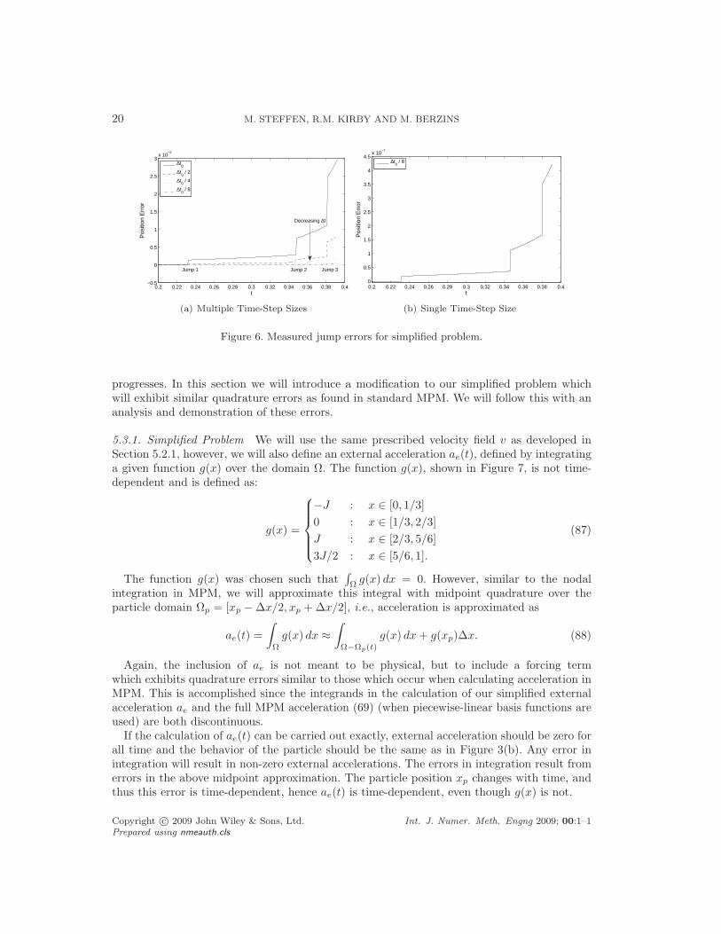
20 M. STEFFEN, R.M. KIRBY AND M. BERZINS
0.2 0.22 0.24 0.26 0.28 0.3 0.32 0.34 0.36 0.38 0.4−0.5
0
0.5
1
1.5
2
2.5
3x 10
−5
t
Pos
ition
Err
or
∆t
0
∆t0 / 2
∆t0 / 4
∆t0 / 8
Decreasing ∆t
Jump 1 Jump 2 Jump 3
(a) Multiple Time-Step Sizes
0.2 0.22 0.24 0.26 0.28 0.3 0.32 0.34 0.36 0.38 0.40
0.5
1
1.5
2
2.5
3
3.5
4
4.5x 10
−7
t
Pos
ition
Err
or
∆t
0 / 8
(b) Single Time-Step Size
Figure 6. Measured jump errors for simplified problem.
progresses. In this section we will introduce a modification to our simplified problem whichwill exhibit similar quadrature errors as found in standard MPM. We will follow this with ananalysis and demonstration of these errors.
5.3.1. Simplified Problem We will use the same prescribed velocity field v as developed inSection 5.2.1, however, we will also define an external acceleration ae(t), defined by integratinga given function g(x) over the domain Ω. The function g(x), shown in Figure 7, is not time-dependent and is defined as:
g(x) =
−J : x ∈ [0, 1/3]
0 : x ∈ [1/3, 2/3]
J : x ∈ [2/3, 5/6]
3J/2 : x ∈ [5/6, 1].
(87)
The function g(x) was chosen such that∫
Ωg(x) dx = 0. However, similar to the nodal
integration in MPM, we will approximate this integral with midpoint quadrature over theparticle domain Ωp = [xp − ∆x/2, xp + ∆x/2], i.e., acceleration is approximated as
ae(t) =
∫
Ω
g(x) dx ≈∫
Ω−Ωp(t)
g(x) dx + g(xp)∆x. (88)
Again, the inclusion of ae is not meant to be physical, but to include a forcing termwhich exhibits quadrature errors similar to those which occur when calculating acceleration inMPM. This is accomplished since the integrands in the calculation of our simplified externalacceleration ae and the full MPM acceleration (69) (when piecewise-linear basis functions areused) are both discontinuous.
If the calculation of ae(t) can be carried out exactly, external acceleration should be zero forall time and the behavior of the particle should be the same as in Figure 3(b). Any error inintegration will result in non-zero external accelerations. The errors in integration result fromerrors in the above midpoint approximation. The particle position xp changes with time, andthus this error is time-dependent, hence ae(t) is time-dependent, even though g(x) is not.
Copyright c© 2009 John Wiley & Sons, Ltd. Int. J. Numer. Meth. Engng 2009; 00:1–1Prepared using nmeauth.cls

DECOUPLING AND BALANCING OF SPACE AND TIME ERRORS IN MPM 21
0 0.1 0.2 0.3 0.4 0.5 0.6 0.7 0.8 0.9 1−1.5
−1
−0.5
0
0.5
1
1.5
2
x
g(x)
g(x) = −J x ∈ [0,1/3]
g(x) = 0 x ∈ [1/3,2/3]
g(x) = J x ∈ [2/3,5/6]
g(x) = 3J/2 x ∈ [5/6,1]
Figure 7. Function g(x) used in calculating external acceleration for a simplified problem.
Finally, we can see the behavior of this system by performing the following Forward-Eulertime-integration strategy
ake =
∫
Ω−Ωp
g(x) dx + g(xkp)∆x (89)
vk+1e = vk
e + ake∆t (90)
vk+1 = v(xkp) + vk+1
e (91)
xk+1p = xk
p + vk+1∆t. (92)
The MPM algorithm exhibits similar behavior as seen in this simplified problem due toquadrature errors in calculating internal forces (16). This complicated interplay between spatialand temporal errors is one reason why analysis of MPM is not straightforward.
5.3.2. Analysis Analysis of quadrature errors in the MPM framework [11] calculated errorsin internal force when evenly spaced particles sample a material with constant stress:
Ef =
∫
Ω
σ(x) · ∇φi dΩ −∑
p
σp · ∇φipVp = σ ·[
∫
Ω
∇φi dΩ − ∆x∑
p
∇φip
]
, (93)
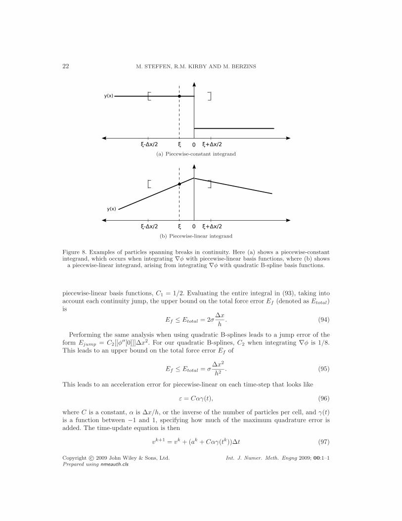
where ∆x is the particle spacing, or volume. Here, ∇φi is either piecewise-constant or piecewise-linear depending on if piecewise-linear or quadratic B-spline basis functions are used. Thebracketed term is equivalent to the error in integrating a piecewise-constant or piecewise-linear function using a composite midpoint rule. This error should be zero if particle voxelsalign with breaks in continuity of the integrand; however, in general this is not the case withMPM. Figure 8 shows an example of a particle spanning breaks in continuity.
The maximum internal force error from Equation (93) when using piecewise-linear basisfunctions is due to integrating over breaks in continuity of the piecewise-constant function∇φ, as can be seen in Figure 8(a). This error looks like Ejump = C1[[φ
′(0)]]∆x, where [[·]]denotes the jump condition, and C1 is a constant depending on the integrand. For the case of
Copyright c© 2009 John Wiley & Sons, Ltd. Int. J. Numer. Meth. Engng 2009; 00:1–1Prepared using nmeauth.cls
22 M. STEFFEN, R.M. KIRBY AND M. BERZINS
(a) Piecewise-constant integrand
(b) Piecewise-linear integrand
Figure 8. Examples of particles spanning breaks in continuity. Here (a) shows a piecewise-constantintegrand, which occurs when integrating ∇φ with piecewise-linear basis functions, where (b) shows
a piecewise-linear integrand, arising from integrating ∇φ with quadratic B-spline basis functions.
piecewise-linear basis functions, C1 = 1/2. Evaluating the entire integral in (93), taking intoaccount each continuity jump, the upper bound on the total force error Ef (denoted as Etotal)is
Ef ≤ Etotal = 2σ∆x
h. (94)
Performing the same analysis when using quadratic B-splines leads to a jump error of theform Ejump = C2[[φ
′′[0]]]∆x2. For our quadratic B-splines, C2 when integrating ∇φ is 1/8.This leads to an upper bound on the total force error Ef of
Ef ≤ Etotal = σ∆x2
h2. (95)
This leads to an acceleration error for piecewise-linear on each time-step that looks like
ε = Cαγ(t), (96)
where C is a constant, α is ∆x/h, or the inverse of the number of particles per cell, and γ(t)is a function between −1 and 1, specifying how much of the maximum quadrature error isadded. The time-update equation is then
vk+1 = vk + (ak + Cαγ(tk))∆t (97)
Copyright c© 2009 John Wiley & Sons, Ltd. Int. J. Numer. Meth. Engng 2009; 00:1–1Prepared using nmeauth.cls

DECOUPLING AND BALANCING OF SPACE AND TIME ERRORS IN MPM 23
xk+1 = xk + vk+1∆t (98)
= xk + vk∆t + ak∆t2 + Cαγ(tk)∆t2 (99)
where the term Cαγ(t)∆t2 is the error term. Continuing, assuming another error in accelerationon the next time-step, we get the following:
vk+2 = vk+1 + (ak+1 + Cαγ(tk+1))∆t (100)
= vk + ak∆t + Cαγ(tk)∆t + ak+1∆t + Cαγ(tk+1)∆t. (101)
Now, let us assume γ(t) is the worst possible case for all t, that is |γ(t)| = 1. Then
vk+2 = vk + ak∆t + ak+1∆t + 2Cα∆t (102)
xk+2 = xk+1 + vk+2∆t (103)
= xk + vk∆t + ak∆t2 + Cα∆t2 + vk∆t + ak∆t2 + ak+1∆t2 + 2Cα∆t2 (104)
= xk + 2vk∆t + 2ak∆t2 + 3Cα∆t2. (105)
If we continue our time steps inductively, we get the following after N steps:
vN = v0 +N
∑
i=1
ai∆t + NCα∆t (106)
xN = x0 +
N∑
j=1
vj∆t (107)
= x0 + Nv0∆t +
N∑
j=1
[
(
j∑
i=1
ai∆t) + jCα∆t
]
∆t (108)
= x0 + Tv0 +
N∑
j=1
j∑
i=1
ai∆t2 +
N∑
j=1
jCα∆t2 (109)
= x0 + Tv0 +N
∑
i=1
(N − i + 1)ai∆t2 +N(N + 1)
2Cα∆t2 (110)
= x0 + Tv0 +
N∑
i=1
(N − i + 1)ai∆t2 +1
2TCα∆t +
1
2T 2Cα, (111)
where T is the final time T = t0 +N∆t. The global quadrature errors with piecewise-constantg(x) is then
Eq =1
2TCα∆t +
1
2T 2Cα. (112)
When piecewise-quadratic basis functions are used, such as B-splines or GIMP functions, theanalysis is similar, leading to global quadrature errors of the form
Eq =1
2TCα2∆t +
1
2T 2Cα2. (113)
Copyright c© 2009 John Wiley & Sons, Ltd. Int. J. Numer. Meth. Engng 2009; 00:1–1Prepared using nmeauth.cls
24 M. STEFFEN, R.M. KIRBY AND M. BERZINS
Our simplified problem with piecewise-linear f will exhibit similar error behavior as theanalysis above for MPM with piecewise-linear basis functions. The following section will showa demonstration of these errors in the simplified problem.
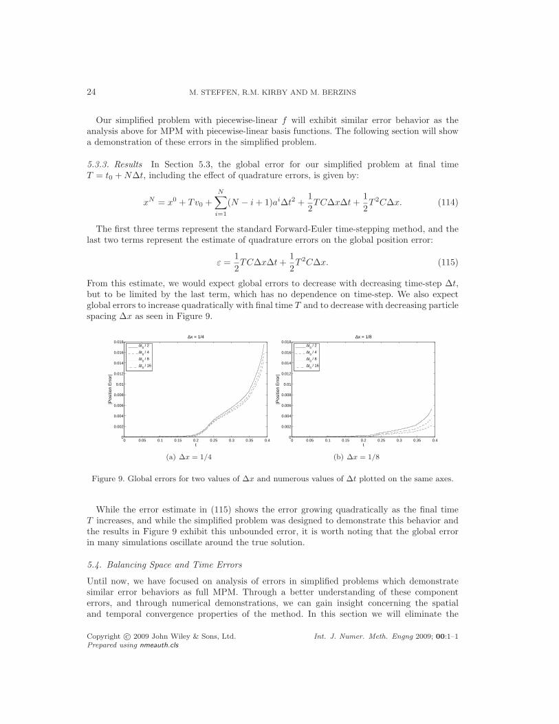
5.3.3. Results In Section 5.3, the global error for our simplified problem at final timeT = t0 + N∆t, including the effect of quadrature errors, is given by:
xN = x0 + Tv0 +N
∑
i=1
(N − i + 1)ai∆t2 +1
2TC∆x∆t +
1
2T 2C∆x. (114)
The first three terms represent the standard Forward-Euler time-stepping method, and thelast two terms represent the estimate of quadrature errors on the global position error:
ε =1
2TC∆x∆t +
1
2T 2C∆x. (115)
From this estimate, we would expect global errors to decrease with decreasing time-step ∆t,but to be limited by the last term, which has no dependence on time-step. We also expectglobal errors to increase quadratically with final time T and to decrease with decreasing particlespacing ∆x as seen in Figure 9.
0 0.05 0.1 0.15 0.2 0.25 0.3 0.35 0.40
0.002
0.004
0.006
0.008
0.01
0.012
0.014
0.016
0.018∆x = 1/4
t
|Pos
ition
Err
or|
∆t
0 / 2
∆t0 / 4
∆t0 / 8
∆t0 / 16
(a) ∆x = 1/4
0 0.05 0.1 0.15 0.2 0.25 0.3 0.35 0.40
0.002
0.004
0.006
0.008
0.01
0.012
0.014
0.016
0.018∆x = 1/8
t
|Pos
ition
Err
or|
∆t
0 / 2
∆t0 / 4
∆t0 / 8
∆t0 / 16
(b) ∆x = 1/8
Figure 9. Global errors for two values of ∆x and numerous values of ∆t plotted on the same axes.
While the error estimate in (115) shows the error growing quadratically as the final timeT increases, and while the simplified problem was designed to demonstrate this behavior andthe results in Figure 9 exhibit this unbounded error, it is worth noting that the global errorin many simulations oscillate around the true solution.
5.4. Balancing Space and Time Errors
Until now, we have focused on analysis of errors in simplified problems which demonstratesimilar error behaviors as full MPM. Through a better understanding of these componenterrors, and through numerical demonstrations, we can gain insight concerning the spatialand temporal convergence properties of the method. In this section we will eliminate the
Copyright c© 2009 John Wiley & Sons, Ltd. Int. J. Numer. Meth. Engng 2009; 00:1–1Prepared using nmeauth.cls

DECOUPLING AND BALANCING OF SPACE AND TIME ERRORS IN MPM 25
compounding of errors in MPM by focusing on single time-step, local truncation errors in thefull MPM framework. Using models for the expected behavior of spatial and temporal errors,we will be able to estimate the balancing point (a particular time-step ∆t) where these twoerrors are equal.
5.4.1. Moving-Mesh MPM The velocity update equation in Equation (64) is astraightforward second-order discretization of v = a. This can be seen by performing Taylorseries expansions of v about time tk:
vk+1/2 =vk + vk(∆t/2) +1
2vk(∆t/2)2 +
1
6
...v k(∆t/2)3 + O(∆t)4 (116)
vk−1/2 =vk − vk(∆t/2) +1
2vk(∆t/2)2 − 1
6
...v k(∆t/2)3 + O(∆t)4. (117)
Subtracting (117) from (116) yields:
vk+1/2 − vk−1/2 = ∆tvk +1
24∆t3
...v k + · · · . (118)
Rearranging terms elucidates to us how this discretization is second-order in time, assuminga is sufficiently smooth:
ak = vk =vk+1/2 − vk−1/2
∆t+ O(∆t2). (119)
And lastly, if we measure local truncation errors, we would expect to see third-order behavior:
vk+1/2 = vk−1/2 + ∆tak + O(∆t3). (120)
Again, these are standard ODE theory results and assume a is known and sufficientlysmooth [23]. However, as was shown above, significant spatial errors can exist in MPM. Infact, assuming second-order spatial errors, acceleration will take the form
ak = ak + c1h2, (121)
where a is our calculated acceleration and c1 is a constant not dependent on h. Substituting(121) into (120) gives us our MPM time-update equation for the centered difference velocityupdate scheme:
vk+1/2 = vk−1/2 + ∆t(ak + c1h2) + c2∆t3. (122)
Here, the term c1h2∆t represents the spatial contribution to the local truncation error. The
term c2∆t3 is the temporal contribution to the local truncation error. Thus, we would expecta transition point between spatial and temporal errors dominating when
c1h2 = c2∆t2 (123)
which occurs when
∆t = Ch, (124)
with C =√
c1/c2.
Copyright c© 2009 John Wiley & Sons, Ltd. Int. J. Numer. Meth. Engng 2009; 00:1–1Prepared using nmeauth.cls

26 M. STEFFEN, R.M. KIRBY AND M. BERZINS
5.4.2. Standard MPM When using standard MPM with piecewise-linear basis functions, weexpect first-order spatial errors. Therefore, instead of (121), acceleration will now be:
ak = ak + c1h, (125)
where a is the calculated acceleration. Substituting (125) into (120) gives us our MPM time-update equation for the centered difference velocity update scheme within the standard MPMframework:
vk+1/2 = vk−1/2 + ∆t(ak + c1h) + c2∆t3. (126)
This differs from (122) in that the spatial error term is first-order, rather than second-order.We would now expect the transition point between spatial and temporal errors dominating at
c1h = c2∆t2, (127)
which occurs when∆t = C
√h, (128)
with C =√
c1/c2.Quadratic B-spline basis functions, however, still exhibit second-order spatial errors for
this problem, even with standard MPM. Therefore, instead of (128), the transition point forstandard MPM with B-spline basis functions should still occur when ∆t = Ch, as in (124).
Demonstrations of these transition, or balancing points will be shown in Section 6.4 for bothmoving-mesh and standard MPM.
6. RESULTS FOR FULL MPM SIMULATIONS
In Section 5, we studied, analyzed, and demonstrated various errors on simplified and decoupledproblems. These problems were chosen due to their relative ease of analysis and becausethey exhibit similar errors to those that exist in a full MPM simulation. In this section, wedemonstrate that these same errors exist in a full MPM simulation and have similar behaviors.
6.1. One-D Periodic Bar
To allow for quantitative measurements of errors, a one-dimensional transient problem with ananalytic solution will be used to perform numerical tests. We will use the same one-dimensionalperiodic bar we have used in previous MPM tests [12]. The problem we are considering has anassumed analytical displacement on the domain [0, 1], and resultant deformation gradient of:
u(X, t) = A sin(2πX) cos(Cπt), (129)
F (X, t) = 1 + 2Aπ cos(2πX) cos(Cπt), (130)
where X is the material position in the reference configuration, A is the maximum deformationpercentage, and C =
√
E/ρ0 is the wave speed. The bar is subjected to a body force of
b(X, t) = C2π2u(X, t)(2F (X, t)−2 + 1). (131)
The functions u and F are included in (131) only to simplify notation. The constitutive modelis a simple 1-D neo-Hookean model, assuming zero Poisson’s ratio:
σ =E
2
(
F − 1
F
)
. (132)
Copyright c© 2009 John Wiley & Sons, Ltd. Int. J. Numer. Meth. Engng 2009; 00:1–1Prepared using nmeauth.cls
DECOUPLING AND BALANCING OF SPACE AND TIME ERRORS IN MPM 27
This constitutive model, when combined with the body force given by (131) will lead to theanalytical displacement solution in (129). We take advantage of the equivalence between the1st Piola-Kirkhhoff and Cauchy stresses in 1-D in the implementation of this test problem.
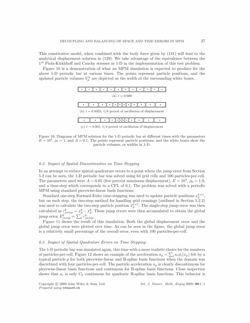
Figure 10 is a demonstration of what an MPM simulation is expected to produce for theabove 1-D periodic bar at various times. The points represent particle positions, and theupdated particle volumes V k
p are depicted as the width of the surrounding white boxes.
(a) t = 0.000
(b) t = 0.0025, 1/8 period of oscillation of displacement
(c) t = 0.005, 1/4 period of oscillation of displacement
Figure 10. Diagrams of MPM solution for the 1-D periodic bar at different times with the parametersE = 104, ρ0 = 1, and A = 0.1. The points represent particle positions, and the white boxes show the
particle volumes, or widths in 1-D.
6.2. Impact of Spatial Discontinuities on Time Stepping
In an attempt to reduce spatial quadrature errors to a point where the jump error from Section5.2 can be seen, the 1-D periodic bar was solved using 64 grid cells and 100 particles-per-cell.The parameters used were A = 0.05 (five percent maximum displacement), E = 104, ρ0 = 1.0,and a time-step which corresponds to a CFL of 0.1. The problem was solved with a periodicMPM using standard piecewise-linear basis functions.
Standard one-step Forward-Euler time-stepping was used to update particle positions xk+1p ,
but on each step, the two-step method for handling grid crossings (outlined in Section 5.2.2)was used to calculate the two-step particle position xk+1
p . The single-step jump error was then
calculated as εkjump = xk
p − xkp. These jump errors were then accumulated to obtain the global
jump error Ekjump =
∑
k εkjump.
Figure 11 shows the result of this simulation. Both the global displacement error and theglobal jump error were plotted over time. As can be seen in the figure, the global jump erroris a relatively small percentage of the overall error, even with 100 particles-per-cell.
6.3. Impact of Spatial Quadrature Errors on Time Stepping
The 1-D periodic bar was simulated again, this time with a more realistic choice for the numbersof particles-per-cell. Figure 12 shows an example of the acceleration ap =
∑
i aiφi(xp) felt by atypical particle p for both piecewise-linear and B-spline basis functions when the domain wasdiscretized with four particles-per-cell. The particle acceleration ap is clearly discontinuous forpiecewise-linear basis functions and continuous for B-spline basis functions. Close inspectionshows that ai is only C0 continuous for quadratic B-spline basis functions. This behavior is
Copyright c© 2009 John Wiley & Sons, Ltd. Int. J. Numer. Meth. Engng 2009; 00:1–1Prepared using nmeauth.cls

28 M. STEFFEN, R.M. KIRBY AND M. BERZINS
0 0.002 0.004 0.006 0.008 0.01 0.012 0.014 0.016 0.018 0.02
0
10
20x 10
−5
t
|Err
or|
Displacement ErrorGlobal Jump Error
Figure 11. Displacement error and cumulative jump error (calculated as the sum of the differencebetween single step and two-step time integration) for a single typical particle in a simulation with 64
grid cells and 100 particles-per-cell.
mainly due to the quadrature errors generated as particles cross grid nodes. This jump inacceleration is unaffected by time-step selection.
0.5 1 1.5 2 2.5 3 3.5 4 4.5
x 10−3
−6000
−5500
−5000
−4500
−4000
−3500
−3000
−2500
−2000
−1500
−1000
−500
t
a
LinearQuadratic B−splineTrue
Figure 12. Acceleration felt by a particle for both piecewise-linear and B-spline basis functions instandard MPM. Discontinuities in accelerations occur at grid crossings with piecewise-linear basisfunctions. With B-spline basis functions, acceleration remains continuous when particles cross grid
nodes.
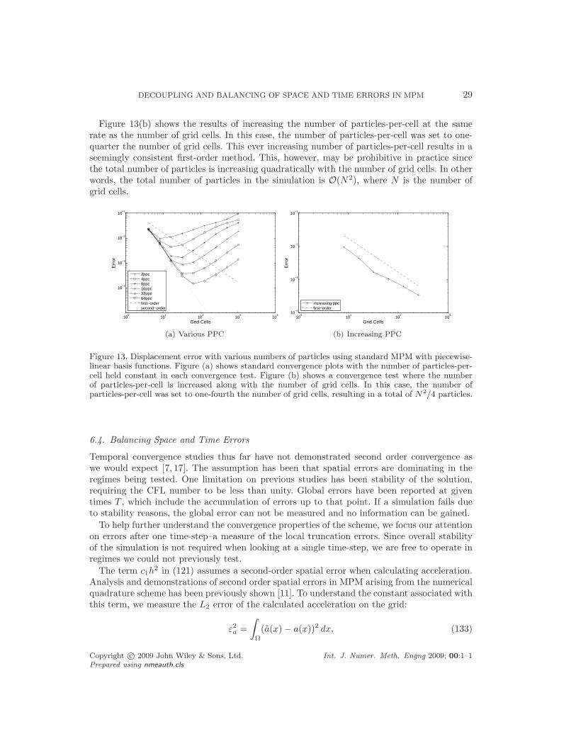
Spatial convergence studies were then performed on the 1-D bar with various numbers ofparticles-per-cell, and the RMS displacement error was calculated after one full period ofoscillation. When the number of particles-per-cell is held constant, standard MPM initiallyconverges at as O(h2), as would be expected in standard finite elements with piecewise-linear basis functions, but soon reaches a point where quadrature error starts to dominate,and convergence is lost. Increasing the number of particles-per-cell lowers the point at whichquadrature errors start to dominate. Figure 13(a) shows these results.
Copyright c© 2009 John Wiley & Sons, Ltd. Int. J. Numer. Meth. Engng 2009; 00:1–1Prepared using nmeauth.cls
DECOUPLING AND BALANCING OF SPACE AND TIME ERRORS IN MPM 29
Figure 13(b) shows the results of increasing the number of particles-per-cell at the samerate as the number of grid cells. In this case, the number of particles-per-cell was set to one-quarter the number of grid cells. This ever increasing number of particles-per-cell results in aseemingly consistent first-order method. This, however, may be prohibitive in practice sincethe total number of particles is increasing quadratically with the number of grid cells. In otherwords, the total number of particles in the simulation is O(N2), where N is the number ofgrid cells.
100
101
102
103
104
10−4
10−3
10−2
10−1
Grid Cells
Err
or
2ppc4ppc8ppc16ppc32ppc64ppcfirst−ordersecond−order
(a) Various PPC
100
101
102
103
10−4
10−3
10−2
10−1
Grid Cells
Err
or
increasing ppcfirst−order
(b) Increasing PPC
Figure 13. Displacement error with various numbers of particles using standard MPM with piecewise-linear basis functions. Figure (a) shows standard convergence plots with the number of particles-per-cell held constant in each convergence test. Figure (b) shows a convergence test where the numberof particles-per-cell is increased along with the number of grid cells. In this case, the number ofparticles-per-cell was set to one-fourth the number of grid cells, resulting in a total of N2/4 particles.
6.4. Balancing Space and Time Errors
Temporal convergence studies thus far have not demonstrated second order convergence aswe would expect [7, 17]. The assumption has been that spatial errors are dominating in theregimes being tested. One limitation on previous studies has been stability of the solution,requiring the CFL number to be less than unity. Global errors have been reported at giventimes T , which include the accumulation of errors up to that point. If a simulation fails dueto stability reasons, the global error can not be measured and no information can be gained.
To help further understand the convergence properties of the scheme, we focus our attentionon errors after one time-step–a measure of the local truncation errors. Since overall stabilityof the simulation is not required when looking at a single time-step, we are free to operate inregimes we could not previously test.
The term c1h2 in (121) assumes a second-order spatial error when calculating acceleration.
Analysis and demonstrations of second order spatial errors in MPM arising from the numericalquadrature scheme has been previously shown [11]. To understand the constant associated withthis term, we measure the L2 error of the calculated acceleration on the grid:
ε2a =
∫
Ω
(a(x) − a(x))2 dx, (133)
Copyright c© 2009 John Wiley & Sons, Ltd. Int. J. Numer. Meth. Engng 2009; 00:1–1Prepared using nmeauth.cls

30 M. STEFFEN, R.M. KIRBY AND M. BERZINS
where a is the true acceleration field from our manufactured solution and a is the calculatedfield:
a(x) =∑
i
aiφi(x). (134)
Figure 14 shows the spatial convergence of these acceleration errors with both piecewise-linearand quadratic B-spline basis functions at a time corresponding to approximately 1/10 theperiod of oscillation (specifically at time t = 0.2122 · C). This time was chosen such thatparticles will have non-zero displacements and velocities.
102
103
104
10−5
10−4
10−3
10−2
10−1
100
101
Grid Cells
Err
or
Piecewise−LinearQuadratic B−splineSecond Order
Figure 14. Spatial convergence of grid acceleration L2 errors at time t = 0.2122 · C, with moving-mesh MPM, four particles-per-cell (PPC), and periodic boundary conditions for the 1D axis aligned
problem.
Again, assuming the acceleration error takes the form εa = c1h2, and since the data in Figure
14 is clearly second order, we can choose one point to calculate the value of c1 for our test case.For example, the acceleration error at 1024 grid cells with piecewise-linear basis functions iscalculated to be 1.7895× 10⁻². Thus, the constant c1 (since our domain is of length L = 1) is
c1 =εa
h2= 1.8764 × 10⁴. (135)
Next, to measure the constant c2, we measured the L2 errors in grid velocity after asingle time-step. The data in Figure 15 shows third-order temporal convergence for the localtruncation error as expected from (122). Knowing that the local velocity truncation errortakes the form εv = c2∆t3, we can choose one point to calculate the value of c2 for our testcase. With piecewise-linear basis functions, the velocity error corresponding to a time-step of∆t = 1.0 × 10⁻⁴ is 1.1277 × 10⁻⁵. This leads to a value for c2 of
c2 =εv
∆t3= 1.1277 × 10⁷. (136)
Copyright c© 2009 John Wiley & Sons, Ltd. Int. J. Numer. Meth. Engng 2009; 00:1–1Prepared using nmeauth.cls

DECOUPLING AND BALANCING OF SPACE AND TIME ERRORS IN MPM 31
10−7
10−6
10−5
10−4
10−3
10−14
10−12
10−10
10−8
10−6
10−4
10−2
∆t
Err
or
Piecewise−LinearQuadratic B−splineThird Order
Figure 15. Temporal convergence of local truncation errors in grid velocity with moving-mesh MPM,220 grid cells, four particles per cell (PPC), and periodic boundary conditions for the 1D axis aligned
problem.
Running a single time-step with 2048 grid cells, (h = 4.88 × 10⁻⁴), we would expect thetransition to occur from (124) at ∆t = 1.9917×10⁻⁵. Figure 16 shows this experiment and thetransition occurs precisely where we expect. Using the same techniques above with the datain Figures 14 and 15, we calculate the transition to occur at ∆t = 2.3908× 10⁻⁵ with B-splinebasis functions. These transition points are very similar, which should not be surprising sincethe errors for piecewise-linear and quadratic B-splines are comparable.
6.4.1. Standard MPM Figure 17 shows the spatial convergence of acceleration errors withstandard MPM. Here, piecewise-linear basis functions initially exhibit second-order spatialconvergence with smaller numbers of grid cells when approximation, or mass-lumping errorsare dominating. However, the asymptotic O(h) quadrature errors eventually dominate whenenough grid cells are used. Quadratic B-spline basis functions still exhibit the expected second-order spatial convergence with standard MPM.
Since the acceleration error for piecewise-linear basis functions now takes the form εa = c1hin the asymptotic region, and since the data in Figure 17 demonstrates that behavior, we canchoose one point to calculate the value of c1 for our test case. For the four particle-per-cellcase, the acceleration error at 1024 grid cells is calculated to be 5.9119× 10⁻². Therefore, theconstant c1 is
c1 =εa
h= 6.0538 × 101. (137)
Next, we again measure the constant c2 using the errors in grid velocity after a single time-step. The data in Figure 18 shows strong third-order local truncation error convergence withlarger ∆t, as expected from (126). With smaller ∆t, a convergence plateau is reached, wherethe larger spatial errors in standard MPM are starting to dominate. Since the local velocity
Copyright c© 2009 John Wiley & Sons, Ltd. Int. J. Numer. Meth. Engng 2009; 00:1–1Prepared using nmeauth.cls
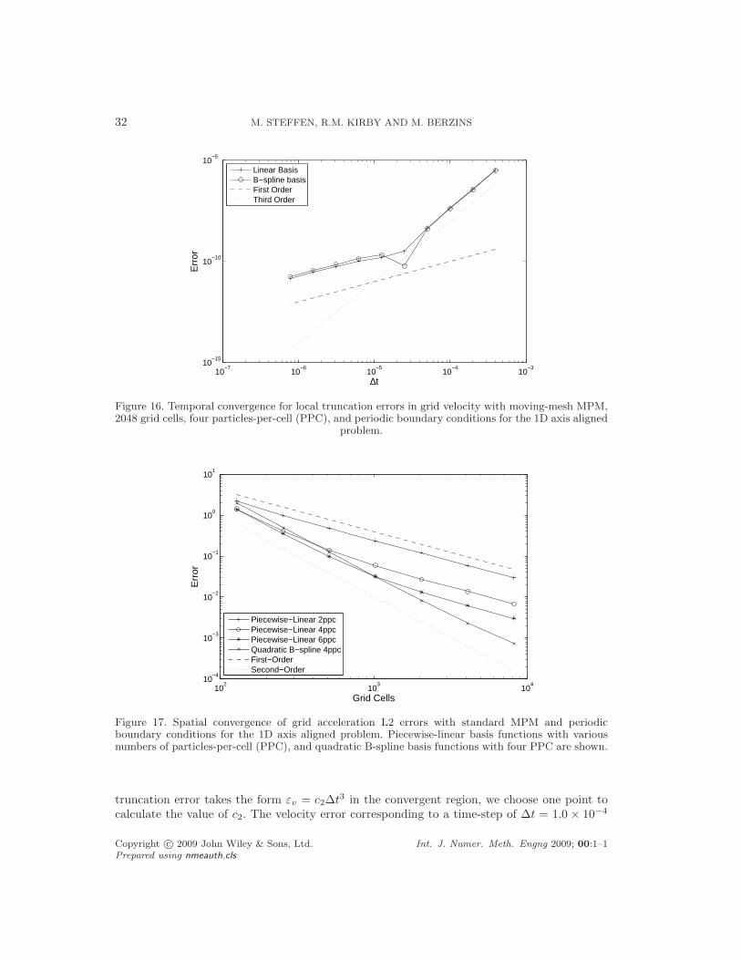
32 M. STEFFEN, R.M. KIRBY AND M. BERZINS
10−7
10−6
10−5
10−4
10−3
10−15
10−10
10−5
∆t
Err
or
Linear BasisB−spline basisFirst OrderThird Order
Figure 16. Temporal convergence for local truncation errors in grid velocity with moving-mesh MPM,2048 grid cells, four particles-per-cell (PPC), and periodic boundary conditions for the 1D axis aligned
problem.
102
103
104
10−4
10−3
10−2
10−1
100
101
Grid Cells
Err
or
Piecewise−Linear 2ppcPiecewise−Linear 4ppcPiecewise−Linear 6ppcQuadratic B−spline 4ppcFirst−OrderSecond−Order
Figure 17. Spatial convergence of grid acceleration L2 errors with standard MPM and periodicboundary conditions for the 1D axis aligned problem. Piecewise-linear basis functions with variousnumbers of particles-per-cell (PPC), and quadratic B-spline basis functions with four PPC are shown.
truncation error takes the form εv = c2∆t3 in the convergent region, we choose one point tocalculate the value of c2. The velocity error corresponding to a time-step of ∆t = 1.0 × 10⁻⁴
Copyright c© 2009 John Wiley & Sons, Ltd. Int. J. Numer. Meth. Engng 2009; 00:1–1Prepared using nmeauth.cls
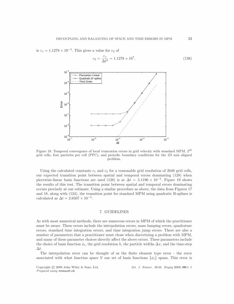
DECOUPLING AND BALANCING OF SPACE AND TIME ERRORS IN MPM 33
is εv = 1.1278 × 10⁻⁵. This gives a value for c2 of
c2 =εv
∆t3= 1.1278 × 10⁷. (138)
10−7
10−6
10−5
10−4
10−3
10−9
10−8
10−7
10−6
10−5
10−4
10−3
∆t
Err
or
Piecewise−LinearQuadratic B−splineThird Order
Figure 18. Temporal convergence of local truncation errors in grid velocity with standard MPM, 220
grid cells, four particles per cell (PPC), and periodic boundary conditions for the 1D axis alignedproblem.
Using the calculated constants c1 and c2 for a reasonable grid resolution of 2048 grid cells,our expected transition point between spatial and temporal errors dominating (128) whenpiecewise-linear basis functions are used (128) is at ∆t = 5.1196 × 10⁻⁵. Figure 19 showsthe results of this test. The transition point between spatial and temporal errors dominatingoccurs precisely at our estimate. Using a similar procedure as above, the data from Figures 17and 18, along with (124), the transition point for standard MPM using quadratic B-splines iscalculated as ∆t = 2.6507 × 10⁻⁵.
7. GUIDELINES
As with most numerical methods, there are numerous errors in MPM of which the practitionermust be aware. These errors include the interpolation errors, mass lumping errors, quadratureerrors, standard time integration errors, and time integration jump errors. There are also anumber of parameters that a practitioner must chose when discretizing a problem with MPM,and many of these parameter choices directly affect the above errors. These parameters includethe choice of basis function φi, the grid resolution h, the particle widths ∆x, and the time-step∆t.
The interpolation error can be thought of as the finite element type error - the errorassociated with what function space V our set of basis functions φi spans. This error is
Copyright c© 2009 John Wiley & Sons, Ltd. Int. J. Numer. Meth. Engng 2009; 00:1–1Prepared using nmeauth.cls

34 M. STEFFEN, R.M. KIRBY AND M. BERZINS
10−7
10−6
10−5
10−4
10−3
10−15
10−10
10−5
∆ t
Err
or
Linear BasisB−spline basisFirst OrderThird Order
Figure 19. Temporal convergence for local truncation errors in grid velocity with standard MPM, 2048grid cells, four particles-per-cell (PPC), and periodic boundary conditions for the 1D axis aligned
problem.
well understood in the context of finite element methods and received little treatment in thispaper. Generally, this error is O(hk) where h is some measure of grid spacing, and k is somemeasure of the order of the basis functions. Thus, both the choice of basis functions and thegrid spacing affect this error. However, even with the simplest piecewise-linear basis functions,this error is O(h2). Increasing the order of basis functions will decrease this error, however thespatial error in MPM is already limited to O(h2) due to other approximations. Therefore theinterpolation error is rarely the limiting factor.
The mass lumping error is also well understood in the context of finite element frameworks[19]. The type of mass lumping employed in MPM is generally considered to provide a O(h2)approximation to the complete (unlumped) mass matrix and is therefore rarely the limitingerror in our simulations. It is important to note that mass lumping can provide positive benefitswith respect to stabilization and monotonicity of the MPM method – things not explored inthis work.
Temporal errors also exist in MPM. The standard time-stepping errors are affected by thechoice of time-step ∆t. In Section 5.2, we focused heavily on the time-stepping jump error– also a function of ∆t, but the smoothness of which is also a function of the basis functionchoice. Smoother basis functions will change the order of this jump error since smoother basisfunctions result in smoother velocity fields that particles travel through.
In Section 5.3 we examined the impact of spatial quadrature errors on time-stepping. Here,the global displacement errors were a function of αk, where α = ∆x/h, and k is again ameasure relating to the smoothness of the basis functions. Increasing the smoothness of thebasis functions from piecewise-linear to piecewise-quadratic (as is the case with the quadraticB-splines used in this paper) increases k from 1 to 2, and since α is typically much less than 1,this significantly reduces the overall effect of quadrature errors on the final global displacement
Copyright c© 2009 John Wiley & Sons, Ltd. Int. J. Numer. Meth. Engng 2009; 00:1–1Prepared using nmeauth.cls

DECOUPLING AND BALANCING OF SPACE AND TIME ERRORS IN MPM 35
error. The choice of ∆t does not affect these quadrature errors.One interesting result is when quadrature errors are dominating (as is often the case
when using piecewise-linear basis functions), the global displacement error looks like αk. Ifthe number of particles-per-cell remains constant, α also remains constant, and the globaldisplacement error will not be reduced as grid resolution is increased. To have a consistentmethod, α must be reduced as grid resolution is increased, meaning the number of particlesper cell must increase as the number of grid cells is increased. A demonstration of this is shownin Section 6.3.
The local truncation error results in Section 6.4 suggest that the time-step, ∆t, where spatialand temporal errors are balanced is much higher than the stability limit when the explicitcentered difference time stepping scheme is used on this type of problem. This explains whyprevious researchers [7] were not able to demonstrate the second-order temporal convergenceexpected from the method in full MPM simulations. Therefore, with a proper implementationof the centered difference time-stepping scheme, time-stepping errors will have generallyconverged to remaining spatial errors by the stability limit, and thus running with a time-stepsignificantly lower than the stability limit has no effect on reducing temporal errors further.
To demonstrate the effects of following these guidelines while solving an engineering problem,the 1-D periodic bar from section 6.1 was simulated with two different sets of parameters. Ina naive attempt at reducing errors, the problem was simulated with piecewise-linear basisfunctions, 128 grid cells, four particles-per-cell, and a relatively small time-step correspondingto a CFL of 0.1. A second simulation used more expensive quadratic B-spline basis functions,64 grid cells, the same four particles-per-cell, and a larger time-step corresponding to a CFLof 0.9. The RMS error of particle positions and corresponding run-times are shown in Table II.Here, we see that a selection of parameters based upon the guidelines provided above resultsin a much lower error with significantly less computational effort.
RMS Error Run-Time (seconds)
Simulation 1 2.21 × 10⁻² 9.62Simulation 2 8.39 × 10⁻⁵ 0.50
Table II. RMS error and run-time for two simulations of a 1D periodic bar. The second simulationmore closely follows the guidelines in this section, resulting in lower error and lower run-time.
8. SUMMARY AND CONCLUSIONS
In this paper we performed three studies on various errors present in the Material PointMethod. These studies, which included analysis and demonstrations, were performed onsimplified problems which exhibit similar error characteristics to the full MPM framework.We also demonstrated these errors in a full MPM simulation. In the process, we have outlinedand demonstrated the moving-mesh MPM algorithm–a fully Lagrangian method which helpscontrol some of the complexities of MPM error analysis, mainly quadrature and grid crossingerrors.
Copyright c© 2009 John Wiley & Sons, Ltd. Int. J. Numer. Meth. Engng 2009; 00:1–1Prepared using nmeauth.cls

36 M. STEFFEN, R.M. KIRBY AND M. BERZINS
The first major error in consideration was the time-stepping jump error, and how spatialdiscontinuities impact these time-stepping errors. We showed that this jump error is second-order with respect to time-step size, and was not a large contributor to the overall globalerrors. The second study focused on the impact of spatial quadrature errors on time-stepping.Building on previous work by the authors, we were able to develop an estimate for globalerrors arising from the compounding effects of the quadrature errors. And lastly, using amodel for the error behavior in the method, we were able to estimate a time-step inflectionpoint where spatial and temporal errors are balanced. Time-steps larger than the inflectionpoint result in solutions dominated by temporal errors, while smaller time steps lead to spatialerror dominated solutions.
These studies allowed us to formulate guidelines for the practitioner when implementing asimilar variant of MPM as used in this paper. The two main guidelines are that the use ofsmoother basis functions (such as quadratic b-splines) greatly reduce the quadrature errors andtherefore reduce global errors in the method, and that time-steps near the stability limit aresufficient in most cases since time-steps near the stability limit already lead to solutions whichare dominated by spatial errors. This helps more fully explain results showing zero-order globaltemporal convergence demonstrated by previous researchers [7]. Further guidelines were given,helping the practitioner understand which algorithm parameters can be expected to affect thevarious errors in the method.
Previous analysis has shown that the nodal integration and the implicit mass lumping inMPM currently restrict the method to second-order in space [11]. To further reduce errors inthe method, more advanced error control techniques beyond simple grid refinement may berequired. Therefore, a detailed understanding of the balance of space and time errors in themethod is key in driving these types of improvements.
9. ACKNOWLEDGMENTS
This work was supported by the U.S. Department of Energy through the Center for theSimulation of Accidental Fires and Explosions (C-SAFE), under grant W-7405-ENG-48. Inaddition, the authors would like to acknowledge helpful discussions with members of the UtahMPM Group – in particular Drs. Jim Guilkey, Phil Wallstedt, and Rebecca Brannon.
REFERENCES
1. D. Sulsky, Z. Chen, and H. L. Schreyer. A particle method for history-dependent materials. ComputerMethods in Applied Mechanics and Engineering, 118:179–196, 1994.
2. D. Sulsky, S. Zhou, and H. L. Schreyer. Application of a particle-in-cell method to solid mechanics.Computer Physics Communications, 87:236–252, 1995.
3. A. D. Brydon, S. G. Bardenhagen, E. A. Miller, and G. T. Seidler. Simulation of the densification of realopen-celled foam microstructures. Journal of the Mechanics and Physics of Solids, 53:2638–2660, 2005.
4. J. A. Nairn. Numerical simulations of transverse compression and densification in wood. Wood and FiberScience, 38(4):576–591, 2006.
5. D. Sulsky, H. Schreyer, K. Peterson, R. Kwok, and M. Coon. Using the material point method to modelsea ice dynamics. Journal of Geophysical Research, 112, 2007.
6. J. E. Guilkey, T. B. Harman, and B. Banerjee. An Eulerian-Lagrangian approach for simulating explosionsof energetic devices. Computers and Structures, 85(11-14):660–674, 2007.
Copyright c© 2009 John Wiley & Sons, Ltd. Int. J. Numer. Meth. Engng 2009; 00:1–1Prepared using nmeauth.cls
DECOUPLING AND BALANCING OF SPACE AND TIME ERRORS IN MPM 37
7. P. C. Wallstedt and J. E. Guilkey. An evaluation of explicit time integration schemes for use with thegeneralized interpolation material point method. Journal of Computational Physics, 227(22):9628–9642,2008.
8. J. U. Brackbill and H. M. Ruppel. FLIP: a method for adaptively zoned, particle-in-cell calculations offluid flows in two dimensions. Journal of Computational Physics, 65:314–343, 1986.
9. J. U. Brackbill, D. B. Kothe, and H. M. Ruppel. FLIP: a low-dissipation, particle-in-cell method for fluidflow. Computer Physics Communications, 48:25–38, 1988.
10. S. G. Bardenhagen and E. M. Kober. The generalized interpolation material point method. ComputerModeling in Engineering and Science, 5(6):477–495, 2004.
11. M. Steffen, R. M. Kirby, and M. Berzins. Analysis and reduction of quadrature errors in the materialpoint method (MPM). International Journal for Numerical Methods in Engineering, 76(6):922–948, 2008.DOI: 10.1002/nme.2360.
12. M. Steffen, P. C. Wallstedt, J. E. Guilkey, R. M. Kirby, and M. Berzins. Examination and analysis ofimplementation choices within the material point method (MPM). Computer Modeling in Engineering &Sciences, 32(2):107–127, 2008.
13. J. E. Guilkey, J. B. Hoying, and J. A. Weiss. Computational modeling of multicellular constructs withthe material point method. Journal of Biomechanics, 39(11):2074–2086, 2006.
14. Liangzhe Zhang. Dynamic description of texture evolution in polycrystalline nickel under mechanicalloading with elastic and plastic deformation via Monte Carlo and Material Point Method simulation.PhD thesis, Colorado School of Mines, 2008.
15. E. Love and D. L. Sulsky. An energy-consistent material-point method for dynamic finite deformationplasticity. International Journal for Numerical Methods in Engineering, 65(10):1608–1638, 2006.
16. E. Love and D. L. Sulsky. An unconditionally stable, energy-momentum consistent implementation of thematerial-point method. Computer Methods in Applied Mechanics and Engineering, 195(33-36):3903–3925,2006.
17. S. Bardenhagen. Energy conservation error in the material point method for solid mechanics. Journal ofComputational Physics, 180:383–403, 2002.
18. J. Lawson, M. Berzins, and P.M. Dew. Balancing space and time errors in the method of lines for parabolicequations. Siam Journal on Scientific and Statistical Computing, 12(3):573–594, 1991.
19. T. J. R. Hughes. The finite element method: linear static and dynamic finite element analysis. Prentice-Hall, 1987.
20. D. Sulsky and A. Kaul. Implicit dynamics in the material-point method. Computer Methods in AppliedMechanics and Engineering, 193(12-14):1137–1170, 2004.
21. J. E. Guilkey and J. A. Weiss. Implicit time integration for the material point method: Quantitative andalgorithmic comparisons with the finite element method. International Journal for Numerical Methodsin Engineering, 57(9):1323–1338, 2003.
22. L. T. Tran, J. Kim, and M. Berzins. Solving Time-Dependent PDEs using the Material Point Method,A Case Study from Gas Dynamics. International Journal for Numerical Methods in Fluids, 2009. DOI:10.1002/nme.2360.
23. E. Hairer, S.P. Nrsett, and G. Wanner. Solving Ordinary Differential Equations I. Springer, 1993.
Copyright c© 2009 John Wiley & Sons, Ltd. Int. J. Numer. Meth. Engng 2009; 00:1–1Prepared using nmeauth.cls