decomposition algorithms for two-stage …

DECOMPOSITION ALGORITHMS FOR TWO-STAGEDISTRIBUTIONALLY ROBUST MIXED BINARY PROGRAMS

MANISH BANSAL∗, KUO-LING HUANG† , AND SANJAY MEHROTRA‡

Abstract. In this paper, we introduce and study a two-stage distributionally robust mixed bi-nary problem (TSDR-MBP) where the random parameters follow the worst-case distribution belong-ing to an uncertainty set of probability distributions. We present a decomposition algorithm, whichutilizes distribution separation procedure and parametric cuts within Benders’ algorithm or L-shapedmethod, to solve TSDR-MBPs with binary variables in the first stage and mixed binary programsin the second stage. We refer to this algorithm as distributionally robust integer (DRI) L-shapedalgorithm. Using similar decomposition framework, we provide another algorithm to solve TSDRlinear problem where both stages have only continuous variables. We investigate conditions and thefamilies of ambiguity set for which our algorithms are finitely convergent. We present two examplesof ambiguity set, defined using moment matching or Kantorovich-Rubinstein distance (Wassersteinmetric), which satisfy the foregoing conditions. We also present a cutting surface algorithm to solveTSDR-MBPs. We computationally evaluate the performance of the DRI L-shaped algorithm andthe cutting surface algorithm in solving distributionally robust versions of a few instances from theStochastic Integer Programming Library, in particular stochastic server location and stochastic mul-tiple binary knapsack problem instances. We also discuss the usefulness of incorporating partialdistribution information in two-stage stochastic optimization problems.

Key words. Distributionally robust optimization; two-stage stochastic mixed binary programs;Benders’ decomposition; L-shaped method; ambiguity set; parametric cutting planes; moment match-ing; Kantorovich-Rubinstein distance; Wasserstein metric.

AMS subject classifications. 90C10, 90C15

1. Introduction. Stochastic programming and robust optimization are well es-tablished optimization models used for making decisions under parametric uncer-tainty. In stochastic programs, it is assumed that the uncertain parameters followa specified probability distribution and an objective function is specified by takingexpectation over these parameters. On the other hand, robust optimization handlesthe uncertainty by solving a minimax problem, where the max is taken over a setof possible values of uncertain parameters. These two competing ideas in decisionmaking under uncertainty can be unified in the framework of distributionally robustoptimization (DRO). In DRO we seek a solution that optimizes the expected value ofthe objective function for the worst case probability distribution within a prescribed(ambiguity) set of distributions that may be followed by the uncertain parameters.Note that in DRO, the exact distribution followed by the uncertain parameters isunknown.

In this paper, we consider a unification of DRO with two-stage stochastic mixedbinary programs (TSS-MBPs), thereby leading to a two-stage distributionally robustoptimization (TSDRO) framework with binary variables in both stages. More specif-ically, we study the following two-stage distributionally robust mixed binary program(TSDR-MBP):

min

cTx+ max

P∈PEξP [Qω(x)]

∣∣∣∣Ax ≥ b, x ∈ 0, 1p.(1)

∗Corresponding author. Grado Department of Industrial and Systems Engineering, Virginia Tech,Blacksburg, VA 24060, USA ([email protected]).†Department of Industrial Engineering and Management Sciences, Northwestern University,

Evanston, IL 60208 ([email protected], [email protected]).

1

mailto:[email protected]



2 MANISH BANSAL, KUO-LING HUANG, AND SANJAY MEHROTRA

where ξP is a random vector defined by probability distribution P with support Ωand for any scenario ω of Ω,

Qω(x) := min gTω yω(2a)

s.t. Wωyω ≥ rω − Tωx(2b)

yω ∈ 0, 1q1 × Rq−q1 .(2c)

We refer to the set of distributions P as the ambiguity set. In (1), the parametersc ∈ Qp, A ∈ Qm1×p, b ∈ Qm1 , and for each ω ∈ Ω, gω ∈ Qq, recourse matrixWω ∈ Qm2×q, technology matrix Tω ∈ Qm2×p, and rω ∈ Qm2 . The formulationdefined by (2) and the function Qω(x) are referred to as the second-stage subproblemand recourse function, respectively.

We assume that

1. X := x : Ax ≥ b, x ∈ 0, 1p is non-empty,2. Kω(x) := yω : (2b)-(2c) hold is non-empty for all x ∈ X and ω ∈ Ω

(relatively complete recourse),3. Each probability distribution P ∈ P has finite support Ω, i.e. |Ω| is finite.

Without loss of generality, we also assume that all elements of the following vectors ormatrices are integer valued (which can be obtained by multiplying these parameterswith appropriate multipliers): c, A, b, and for ω ∈ Ω, gω, Wω, Tω, and rω. Further-more, we assume that there exists an oracle that provides a probability distributionP ∈ P, i.e., pωω∈Ω where pω is the probability of occurrence of scenario ω ∈ Ω, bysolving the optimization problem:

Q(x) := maxP∈P

EξP [Qω(x)](3)

for a given x ∈ X. We refer to this optimization problem as distribution separationproblem corresponding to an ambiguity set, and the algorithm to solve this problemis referred to as the distribution separation algorithm. In Section 1.7, we providetwo examples of ambiguity set and the distribution separation problems associated tothem. To the best of our knowledge, TSDR-MBPs have not been studied before.

1.1. Contributions of this paper. We present a decomposition algorithm,which utilizes distribution separation procedure and parametric cuts within Benders’algorithm [10], to solve TSDR-MBPs. We refer to this algorithm as distributionallyrobust integer (DRI) L-shaped algorithm because it generalizes the well-known integerL-shaped algorithm [27] developed for a special case of TSDR-MBP where P is single-ton. Using similar decomposition framework, we develop a decomposition algorithmfor two-stage distributionally robust linear program, i.e. TSDR-MIP with no binaryrestrictions on both first and second stage variables. Moreover, we provide conditionsand the families of ambiguity set P for which our algorithms are finitely convergent.Furthermore, we present a cutting surface algorithm to solve TSDR-MBPs and com-putationally evaluate the performance of DRI L-shaped algorithm and the cuttingsurface algorithm in solving DR versions of stochastic server location problem andstochastic multiple binary knapsack problem instances from Stochastic Integer Pro-gramming Library (SIPLIB) [1], and stochastic server location problem with randomrecourse [31]. We observe that our DRI L-shaped algorithm solves all these probleminstances to optimality in less than an hour. It is important to note that the TSDR-MBP generalizes various classes of optimization problems studied in literature. Beloware few of them:

ALGORITHMS FOR TWO-STAGE DISTRIBUTIONALLY ROBUST PROGRAMS 3

– Two-Stage Stochastic Mixed Binary Program (TSS-MBP): TSDR-MBP (1)with a singleton P = P0 defines TSS-MBP [21, 27, 40].

– Two-Stage Robust Mixed Binary Program(TSR-MBP): TSDR-MBP (1) witha set P that consists of all probability distributions supported on Ω is equiv-alent to TSR-MBP.

– Distributionally Robust Optimization (DRO): In literature, the general DROproblem [17, 29, 36, 38, 39] is defined as follows:

(4) minx∈X

maxP∈P

EξP [Hω(x)]

where Hω is a random cost or disutility function corresponding to scenario ω.Assuming that X = X and Hω is defined by a mixed binary program, Prob-lem (4) is a special case of TSDR-MBP (i.e., Problem (1)) where c is a vectorof zeros.

– Two-Stage Distributionally Robust Linear Program (TSDR-LP): The TSDR-LP [11, 22, 28] is a relaxation of TSDR-MBP where the both stages have onlycontinuous variables.

Note that the TSDR-MBP is at least as hard as the TSS-MBP (a special caseof TSDR-MBP) which is an #P-hard problem [19]. The remaining section providessignificance of TSDRO framework (Section 1.2), literature review of TSS-MBP, DROframework and TSDR-LP, and ambiguity sets (Section 1.3, 1.4, and 1.5, respectively),and organization of this paper (Section 1.6).

1.2. Significance of TSDRO framework. The ability to allow incompleteinformation on the probability distribution is a major advantage of the TSDRO ap-proach to model formulation. In a two-stage decision framework where future predic-tions are generated using a data driven approach, no assumptions on the knowledgeof prediction error distribution is required. The prediction errors can be empiricallygenerated, and the TSDRO framework can be used to robustify around the empiricalerror distribution. Alternatively, when the uncertain parameters in the model arespecified by uncertainty quantification (UQ) techniques, this framework allows one tomodel errors in UQ without requiring the errors to follow a specified (e.g., normal)distribution. In addition, TSDRO framework provides decision sensitivity analysiswith respect to the reference probability distribution.

One can also view the TSDR-MBP not only as a common generalization of TSR-MBP and TSS-MBP, but also as an optimization model with an adjustable level ofrisk-aversion. To see this, consider a nested sequence of sets of probability distribu-tions P0 ⊇ P1 ⊇ · · · , where P0 is the set of all probability distributions supported on

Ω, and P∞def= ∩∞i=0Pi is a singleton set. In the corresponding sequence of problems

(1), the first one (P = P0) is the TSR-MBP, which is the most conservative (risk-averse) of all, and the last one is the TSS-MBP, where the optimization is againsta fixed distribution. At the intermediate levels the models correspond to decreasinglevels of risk-aversion.

Remark 1. For the sake of reader’s convenience, below we list the abbreviationsused in this paper:

– TSS: Two-stage stochastic– TSR: Two-stage robust– TSDR: Two-stage distributionally robust– MBP: Mixed binary program– LP: Linear program


– MIP: Mixed integer program– DRO: Distributionally robust optimization– DRI: Distributionally robust integer– SSLP: Stochastic server location problem– SMKP: Stochastic multiple binary knapsack problem– SSLPR: SSLP with random recourse– SIPLIB: Stochastic Integer Programming Library

1.3. Literature review of TSS-MBPs. Laporte and Louveaux [27] providethe integer L-shaped algorithm for TSS-MBP by assuming that the second stageproblems are solved to optimality at each iteration. Sherali and Fraticelli [40] considersingle scenario TSS-MBPs, i.e. Ω := ω1. They develop globally valid cuts in (x, yω1

)space using the reformulation-linearization technique. These cuts are then used whilesolving the second stage mixed binary programs for a given x ∈ X and hence the cutsin yω space are referred to as the “parametric” cuts. Likewise, Gade et. al. [21] utilizethe parametric Gomory fractional cuts within Benders’ decomposition algorithm forsolving TSS-MIPs with only binary variables in the first stage and non-negative integervariables in the second stage. To solve TSS-MBPs, different forms of parametric cutshave been used in literature; for instance see [15, 21, 31, 37]. Readers can referto [26] for a comprehensive survey on algorithms for TSS-MBPs and to [13, 42] foralgorithms for TSS-LPs which utilize bounds on expectation of the recourse function[8, 24]. Note that in the aforementioned papers, the parametric cuts are added insuccession. In contrast, Bansal et al. [4] provide conditions under which the secondstage mixed integer programs of two-stage stochastic mixed integer program (TSS-MIP) can be convexified by adding parametric inequalities a priori. They provideexamples of TSS-MIPs which satisfy these conditions by considering parametrizedversions of some structured mixed integer set such as special cases of continuousmulti-mixing set [5, 6], and convex objective integer programs in the second stage.

1.4. Literature review of DRO framework and TSDR-LPs. Scarf [36]introduced the concept of DRO by considering a news vendor problem. Thereafter,this framework has been used to model varieties of problems [9, 18, 20, 33]. Onalgorithmic front for solving DRO problems, Shapiro and Kleywegt [39] and Shapiroand Ahmed [38] provide approaches to derive an equivalent stochastic program witha certain distribution. Delage and Ye [17] give general conditions for polynomial timesolvability of DRO where the ambiguity set is defined by setting constraints on firstand second moments. Using ellipsoidal method, they [17] also show that under certainconditions on the disutility functions Hω and the ambiguity set P, Problem (4) issolvable in polynomial time. Mehrotra and Zhang [30] extend this result by providingpolynomial time methods for distributionally robust least squares problems, usingsemidefinite programming. Mehrotra and Papp [29] develop a central cutting surfacealgorithm for Problem (4) where the ambiguity set is defined using constraints onfirst to fourth moments. Recently, Postek et al. [34] study the DRO problem wherethe ambiguity set is defined using mean-dispersion measures and utilize the resultsof Ben-Tal and Hochman [8], i.e. bounds on expectation of a convex function of arandom variable, to derive algorithms for variants of the DRO problem.

Lately researchers have been considering two-stage stochastic linear programswith ambiguity sets, in particular TSDR-LP [11, 28, 22]. More specifically, Bertsimaset al. [11] consider TSDR-LP where the ambiguity set is defined using multivariatedistributions with known first and second moments and risk is incorporated in themodel using a convex nondecreasing piecewise linear function on the second stage


costs. They show that the corresponding problem has semidefinite programmingreformulations. Jiang and Guan [25] present sample average approximation algorithmto solve a special case of TSDR-MBP with binary variables only in the first stage wherethe ambiguity set is defined using l1-norm on the space of all (continuous and discrete)probability distributions. Recently, Love and Bayraksan [28] develop a decompositionalgorithm for solving TSDR-LP where the ambiguity set is defined using φ-divergence.Whereas Hanasusanto and Kuhn [22] provide a conic programming reformulations forTSDR-LP where the ambiguity set comprises of a 2-Wasserstein ball centered at adiscrete distribution. As per our knowledge, no work has been done to solve TSDR-LP with binary variables in both stages, i.e. TSDR-MBP. In this paper, we developnew decomposition algorithms for TSDR-LP and TSDR-MBP with a general familyof ambiguity sets, and provide conditions and families of ambiguity sets for whichthese algorithms are finitely convergent.

1.5. Literature review of ambiguity sets. Though in this paper we considera general family of ambiguity sets, in literature there exists different ways to constructthe ambiguity set of distributions; refer to [23] and references therein for more details.To begin with, Scarf [36] define the ambiguity set using linear constraints on thefirst two moments of the distribution. Similar ambiguity set is also considered in[12, 18, 35]; whereas Bertsimas et al. [11] and Delage and Ye [17] use conic constraintsto describe the set of distributions with moments, and a more general model allowingbounds on higher order moments has been recently studied in [29]. Other definitionsof the ambiguity sets considered in the literature include the usage of the measurebounds and general moment constraints [30, 38], Kantorovich distance or Wassersteinmetric [30, 32, 33, 45], ζ-structure metrics [48], φ-divergences such as χ2 distanceand Kullback-Leibler divergence [7, 14, 25, 28, 43, 46], and Prokhorov metrics [20].We give two examples of families of ambiguity set in Section 1.7 and also providedistribution separation problem associated to each of the ambiguity sets.

1.6. Organization of this paper. In Section 2, we present a decompositionalgorithm to solve TSDR-LP by embedding distribution separation algorithm (asso-ciated to the ambiguity set) within L-shaped method. We refer to our algorithmas the distributionally robust L-shaped algorithm and provide families of ambiguityset for which it is finitely convergent. In Section 3, we further extend our algo-rithm to solve TSDR-MBPs using parametric cuts, thereby generalizing the integerL-shaped method. We refer to this generalized algorithm as the distributionally ro-bust integer (DRI) L-shaped algorithm. In Section 3.3, we provide conditions andthe families of ambiguity set for which the DRI L-shaped algorithm is finitely con-vergent. Interestingly, the two examples of ambiguity set discussed in Section 1.7satisfy the aforementioned conditions. In Section 3.4, we present a cutting surfacealgorithm where we solve the subproblems to optimality using branch-and-cut ap-proach. Thereafter, in Section 4 we computationally evaluate the performance of theDRI L-shaped algorithm and the cutting surface algorithm in solving distributionallyrobust versions of problem instances taken from the Stochastic Integer ProgrammingLibrary (SIPLIB) [1] and the paper [31]. In particular, we consider instances of thestochastic server location problem (with random recourse) and stochastic multiplebinary knapsack problem. Finally, we give concluding remarks in Section 5.

1.7. Examples of ambiguity set and associated distribution separationprocedures. In this section, we provide two examples of ambiguity sets and thedistribution separation algorithm associated to these sets. These sets, referred to as


the moment matching set (5) and Kantorovich set (7), are defined by polytopes withfinite number of extreme points.

Moment matching set. We define the set P via bounds on some (not neces-sarily polynomial) moments. For a finite sample space Ω := ω1, . . . , ω|Ω|, letv := (v1, . . . , v|Ω|) be the corresponding probability measure. Given continuous basisfunctions f1, . . . , fN defined for (Ω, X) 7→ R, the moment matching set is given by:

(5) PM :=

v ∈ R|Ω|+ : u ≤|Ω|∑l=1

vlf(ωl) ≤ u

,

where u and u are lower and upper bound vectors, respectively, on the correspond-ing moments. In addition, the optimization (or distribution separation) problem (3)associated with PM is a linear program:

(6) maxv∈R|Ω|

|Ω|∑l=1

vlQωl(x)

∣∣∣∣∣∣ u ≤|Ω|∑l=1

vlf(ωl) ≤ u, v ≥ 0

,

where decision variables are the weights vl that the distribution P assigns to eachpoint ωl ∈ Ω for l = 1, . . . , |Ω|.Kantorovich set. The use of Kantorovich-Rubinstein (KR) distance (or Wassersteinmetric) is another important choice in specifying ambiguity in a distribution. Assumethat P∗ is a known reference probability measure and ε > 0 is given. Again, ifΩ := ω1, . . . , ω|Ω| is a finite set, v := (v1, . . . , v|Ω|) is the corresponding probabilitymeasure, and v∗j , j = 1, . . . , |Ω|, are given probabilities corresponding to a referencedistribution defined on the sample space, then the Kantorovich set is given by:

PK :=

v ∈ R|Ω| :

|Ω|∑i=1

|Ω|∑j=1

‖ωi − ωj‖1ki,j ≤ ε,

|Ω|∑j=1

ki,j = vi, i = 1, . . . , |Ω|

|Ω|∑i=1

ki,j = v∗j , j = 1, . . . , |Ω|

|Ω|∑i=1

vi = 1

vi ≥ 0, i = 1, . . . , |Ω|

ki,j ≥ 0, i = 1, . . . , |Ω|, j = 1, . . . , |Ω|,

(7)

and the associated distribution separation problem is given by the following linearprogram:

max

|Ω|∑l=1

vlQωl(x) : v ∈ PK

.(8)


In (8), the decision variables are ki,j and vi for i, j ∈ 1, . . . , |Ω|, and the constraintsare similar to those in a standard transportation problem with an additional inequalityconstraint.

2. Distributionally robust L-shaped algorithm for TSDR-LP. In thissection, we develop a decomposition algorithm which utilizes distribution separationalgorithm within Benders’ method for solving TSDR-LP where the ambiguity set Pis defined by a polytope with a finite number of extreme points (for example, momentmatching set PM and Kantorovich set PK). Recall that TSDR-LP is a relaxation ofTSDR-MBP, i.e. (1), where the both stages have only continuous variables. We referto our algorithm as the distributionally robust L-shaped algorithm. The pseudocodeof this algorithm is given by Algorithm 1. Now, let LB and UB be the lower boundand upper bound, respectively, on the optimal solution value of a given TSDR-LP.We define subproblem Sω(x), for x ∈ XLP := x ∈ Rp : Ax ≥ b and ω ∈ Ω, asfollows:

Qsω(x) := min gTω yω(9a)


yω ∈ Rq.(9c)

Let π∗ω,0(x) ∈ Rm2 be the optimal dual multipliers corresponding to constraints(9b) which are obtained by solving Sω(x) for a given x ∈ XLP and ω ∈ Ω. We derive alower bounding approximation of the linear programming relaxation of the first stageproblem (1) using the following optimality cut, OCS(π∗ω,0(x), pωω∈Ω):

(10)∑ω∈Ω

pω

π∗ω,0(x)T (rω − Tωx)

≤ θ,

where pωω∈Ω is obtained by solving the distribution separation problem associatedto the ambiguity set P. We refer to the lower bound approximation of the first stageproblem (1) as the master problem which is defined by

mincTx+ θ : x ∈ XLP and OCS(π∗ω,0(xk), pkωω∈Ω) holds, for k = 1, . . . , l(11)

where xk ∈ XLP for k = 1 . . . , l, π∗ω,0(xk) is the set of optimal dual multiplier obtained

by solving Sω(xk), ω ∈ Ω, and pkωω∈Ω is the set of probabilities for scenarios insample space Ω obtained by solving distribution separation problem for xk ∈ XLP ,k ∈ 1, . . . , l. We denote this problem by Ml for l ∈ Z+. Note that M0 is themaster problem without any optimality cut.

Now, we initialize Algorithm 1 by setting lower bound LB to negative infinity,upper bound UB to positive infinity, iteration counter l to 1, and by solving M0 toget a first stage feasible solution x1 ∈ XLP (Line 1). At each iteration l ≥ 1, we solvelinear programs Sω(xl) for all ω ∈ Ω and store the corresponding optimal solutiony∗ω(xl) and the optimal solution value Qs

ω(xl) := gTω y∗ω(xl) for each ω ∈ Ω (Lines 3-5).

Next, we solve the distribution separation problem associated to the ambiguity set Pand obtain the optimal solution, i.e. plωω∈Ω (Line 7). Since y∗ω(xl) ∈ Kω(xl) for allω ∈ Ω, we have a feasible solution (xl, y∗ω1

(xl), . . . , y∗ω|Ω|(xl)) for the original problem.

Therefore, using plωω∈Ω, we update UB if the solution value corresponding to thusobtained feasible solution is smaller than the existing upper bound (Lines 8-9). Wealso utilize the stored information and optimal dual multipliers (Line 14) to derive


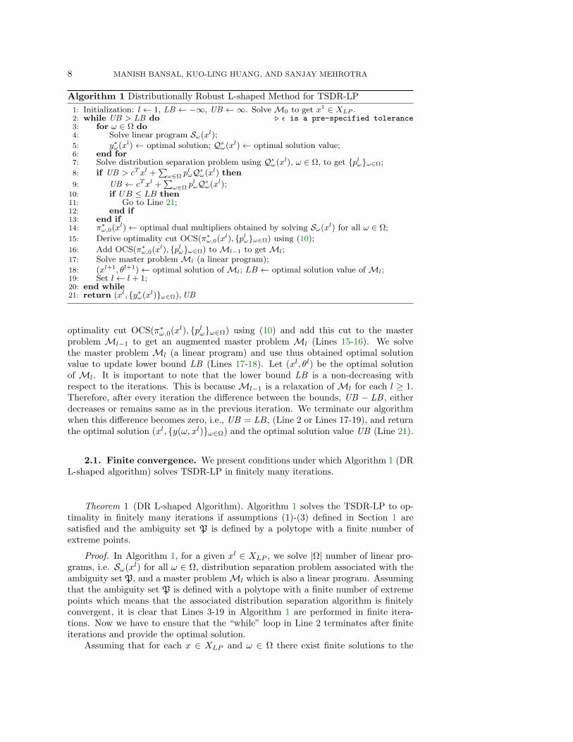
Algorithm 1 Distributionally Robust L-shaped Method for TSDR-LP

1: Initialization: l← 1, LB ← −∞, UB ←∞. Solve M0 to get x1 ∈ XLP .2: while UB > LB do . ε is a pre-specified tolerance3: for ω ∈ Ω do4: Solve linear program Sω(xl);5: y∗ω(xl)← optimal solution; Qs

ω(xl)← optimal solution value;6: end for7: Solve distribution separation problem using Qs

ω(xl), ω ∈ Ω, to get plωω∈Ω;8: if UB > cTxl +

∑ω∈Ω p

lωQs

ω(xl) then

9: UB ← cTxl +∑

ω∈Ω plωQs

ω(xl);10: if UB ≤ LB then11: Go to Line 21;12: end if13: end if14: π∗ω,0(xl)← optimal dual multipliers obtained by solving Sω(xl) for all ω ∈ Ω;

15: Derive optimality cut OCS(π∗ω,0(xl), plωω∈Ω) using (10);

16: Add OCS(π∗ω,0(xl), plωω∈Ω) to Ml−1 to get Ml;17: Solve master problem Ml (a linear program);18: (xl+1, θl+1)← optimal solution of Ml; LB ← optimal solution value of Ml;19: Set l← l + 1;20: end while21: return (xl, y∗ω(xl)ω∈Ω),UB

optimality cut OCS(π∗ω,0(xl), plωω∈Ω) using (10) and add this cut to the masterproblem Ml−1 to get an augmented master problem Ml (Lines 15-16). We solvethe master problem Ml (a linear program) and use thus obtained optimal solutionvalue to update lower bound LB (Lines 17-18). Let (xl, θl) be the optimal solutionof Ml. It is important to note that the lower bound LB is a non-decreasing withrespect to the iterations. This is because Ml−1 is a relaxation of Ml for each l ≥ 1.Therefore, after every iteration the difference between the bounds, UB − LB , eitherdecreases or remains same as in the previous iteration. We terminate our algorithmwhen this difference becomes zero, i.e., UB = LB , (Line 2 or Lines 17-19), and returnthe optimal solution (xl, y(ω, xl)ω∈Ω) and the optimal solution value UB (Line 21).

2.1. Finite convergence. We present conditions under which Algorithm 1 (DRL-shaped algorithm) solves TSDR-LP in finitely many iterations.

Theorem 1 (DR L-shaped Algorithm). Algorithm 1 solves the TSDR-LP to op-timality in finitely many iterations if assumptions (1)-(3) defined in Section 1 aresatisfied and the ambiguity set P is defined by a polytope with a finite number ofextreme points.

Proof. In Algorithm 1, for a given xl ∈ XLP , we solve |Ω| number of linear pro-grams, i.e. Sω(xl) for all ω ∈ Ω, distribution separation problem associated with theambiguity set P, and a master problemMl which is also a linear program. Assumingthat the ambiguity set P is defined with a polytope with a finite number of extremepoints which means that the associated distribution separation algorithm is finitelyconvergent, it is clear that Lines 3-19 in Algorithm 1 are performed in finite itera-tions. Now we have to ensure that the “while” loop in Line 2 terminates after finiteiterations and provide the optimal solution.

Assuming that for each x ∈ XLP and ω ∈ Ω there exist finite solutions to the


second stage programs (Assumptions 1-3 defined in Section 1), we first prove that theoptimality cuts (10) are supporting hyperplanes of Qs(x) := maxP∈P EξP [Qsω(x)] forall x ∈ XLP . Notice that the original problem TSDR-LP is equivalent to

min (cTx+ θ)(12)

s.t. x ∈ XLP(13)

maxP∈P

∑ω∈Ω

pωQsω(x)

≤ θ.(14)

Furthermore, for each xl ∈ XLP ,

Qsω(xl) = π∗ω,0(xl)T(rω − Tωxl

),

and after solving the distribution separation problem for xl, we get

Qs(xl) = maxP∈P

∑ω∈Ω

pωQsω(xl)

=∑ω∈Ω

plωQsω(xl)(15)

=∑ω∈Ω

plω

π∗ω,0(xl)T

(rω − Tωxl

).(16)

Since Qsω(x) is convex in x, EξP [Qω(x)] =∑ω∈Ω pωQsω(x) is convex for a given

probability distribution P ∈ P or pωω∈Ω. This implies Qs(x) is also a convexfunction of x because maximum over an arbitrary collection of convex functions isconvex. Therefore from the subgradient inequality,

Qs(x) = maxP∈P

∑ω∈Ω

pωQsω(x)

≥∑ω∈Ω

plω

π∗ω,0(xl)T (rω − Tωx)

,

and hence from (14), it is clear that∑ω∈Ω

plω

π∗ω,0(xl)T (rω − Tωx)

≤ θ.(17)

Inequalities (17) are same as the optimality cuts OCS(π∗ω,0(xl), plωω∈Ω) and are thesupporting hyperplanes for Qs(x). Also, in (12)-(14), θ is unrestricted except forθ ≥ Qs(x).

Let (xl+1, θl+1) be the optimal solution obtained after solving the master problemMl (11) in Step 17 of Algorithm 1. Then, either of the following two cases will occur:

Case I [θl+1 ≥ Qs(xl+1)]: Observe that (xl+1, θl+1) is a feasible solution to theproblem defined by (12)-(14) because xl+1 ∈ XLP and θl+1 ≥ Qs(xl+1). Interest-ingly, it is also the optimal solution of the problem because if there exists a solution(x∗, θ∗) 6= (xl+1, θl+1) such that cTx∗ + θ∗ < cTxl+1 + θl+1 then (x∗, θ∗) must be theoptimal solution to the master problem Ml. Also,

LB = cTxl+1 + θl+1 ≥ cTxl+1 +∑ω∈Ω

pl+1ω Qsω(xl+1) = UB.

The last inequality satisfies the termination condition in Line 10 and hence, Algorithm1 terminates whenever this case occurs and returns the optimal solution.


Case II [θl+1 < Qs(xl+1)]: Clearly (xl+1, θl+1) is not a feasible solution to theproblem (12)-(14) because constraint (14) is violated by it. Also,

LB = cTxl+1 + θl+1 < cTxl+1 +∑ω∈Ω

pl+1ω Qsω(xl+1) = UB.

Since the termination condition in Line 10 is not satisfied, we derive optimality cutin Line 15 to cut-off the point (xl+1, θl+1).

Next we show that Case II will occur finite number of times in Algorithm 1, whichimplies that the ”while” loop will terminate after finite iterations and will return theoptimal solution. In Case II, θl+1 < Qs(xl+1); it means that none of the previ-ously derived optimality cuts adequately impose Qs(x) ≤ θ at (xl+1, θl+1). Thereforeprobability distribution pl+1

ω ω∈Ω and a new set of dual multipliers π∗ω,0(xl+1)ω∈Ω

are obtained in Lines 7 and 14, respectively, to derive an appropriate optimality cutOCS(π∗ω,0(xl+1), pl+1

ω ω∈Ω) which cut-off the point (xl+1, θl+1). It is important to

note that adding the optimality cut toMl forces θ ≥ Qs(xl+1). Since each dual multi-plier π∗ω,0(x) corresponds to one of the finitely many different basis, there are finitelynumber of the set of dual multiplier. In addition, because of the assumption thatthe ambiguity set P is defined by a polytope with finite number of extreme points,there are finite number of possible solutions pl+1

ω ω∈Ω to the distribution separationalgorithm for xl+1. Hence, there are finite number of optimality cuts. Therefore,after finite iterations with Case II, Case I occurs and Algorithm 1 terminates. Thiscompletes the proof.

3. Distributionally robust integer L-shaped algorithm for TSDR-MBP.In this section, we further generalize the distributionally robust L-shaped algorithm(Algorithm 1) for solving TSDR-MBP using parametric cuts. We refer to this gen-eralized algorithm as the distributionally robust integer L-shaped algorithm. Thepseudocode of our algorithm is given by Algorithm 2. Because of the presence of thebinary variables in both stages, we re-define subproblem Sω(xl), master problemMl,and optimality cuts for Algorithm 2.

First, we define subproblem Sω(x), for x ∈ X and ω ∈ Ω, as follows:

Qsω(x) := min gTω yω(18a)


αtωyω ≥ βtω − ψtωx, t = 1, . . . , τω(18c)

yω ∈ Rq+,(18d)

where αtω ∈ Qq, ψtω ∈ Qp, and βtω ∈ Q are the coefficients of yω, coefficients of x,and the constant term in the right hand side, respectively, of a parametric inequality.We will discuss how these parametric inequalities (more specifically, parametric lift-and-project cuts) are developed in succession for mixed binary second stage problemsin Section 3.1. Also, for a given x ∈ X and ω ∈ Ω, the optimal dual multipliersobtained by solving Sω(x) are defined by π∗ω(x) = (π∗ω,0(x), π∗ω,1(x), . . . , π∗ω,τω (x))T

where π∗ω,0(x) ∈ Rm2 corresponds to constraints (18b) and π∗ω,t(x) ∈ R correspondsto constraint (18c) for t = 1, . . . , τ(ω). In contrast to the previous section, we derivea lower bounding approximation of the first stage problem (1), referred as the masterproblem Ml:

mincTx+ θ : x ∈ X and OCS(π∗ω(xk), pkωω∈Ω) holds, for k = 1, . . . , l,(19)


using the following optimality cut, OCS(π∗ω(x), pωω∈Ω):

(20)∑ω∈Ω

pω

π∗ω,0(x)T (rω − Tωx) +

τω∑t=1

π∗ω,t(x)(βtω − ψtωx

)≤ θ.

Algorithm 2 Distributionally Robust Integer L-shaped Method for TSDR-MBP

1: Initialization: l← 1, LB ← −∞, UB ←∞, τω ← 0 for all ω ∈ Ω. Assume x1 ∈ X.2: while UB − LB > ε do . ε is a pre-specified tolerance3: for ω ∈ Ω do4: Solve linear program Sω(xl);5: y∗ω(xl)← optimal solution; Qs∗

ω (xl)← optimal solution value;6: end for7: if y∗ω(xl) /∈ Kω(xl) for some ω ∈ Ω then8: for ω ∈ Ω where y∗ω(xl) /∈ Kω(xl) do . Add parametric inequalities9: Add the parametric cut to Sω(x) as explained in Section 3.1;

10: Set τω ← τω + 1 and solve linear program Sω(xl);11: y∗ω(xl)← optimal solution; Qs∗

ω (xl)← optimal solution value;12: end for13: end if14: Solve distribution separation problem using Qs∗

ω (xl), ω ∈ Ω, to get plωω∈Ω;15: if y∗ω(xl) ∈ Kω(xl) for all ω ∈ Ω and UB > cTxl +

∑ω∈Ω p

lωQs∗

ω (xl) then

16: UB ← cTxl +∑

ω∈Ω plωQs∗

ω (xl);17: if UB ≤ LB + ε then18: Go to Line 21;19: end if20: end if21: π∗ω(xl)← optimal dual multipliers obtained by solving Sω(xl) for all ω ∈ Ω;22: Derive optimality cut OCS(π∗ω(xl), plωω∈Ω) using (10);23: Add OCS(π∗ω(xl), plωω∈Ω) to Ml−1 to get Ml;24: Solve master problem Ml as explained in Section 3.1;25: (xl+1, θl+1)← optimal solution of Ml; LB ← optimal solution value of Ml;26: Set l← l + 1;27: end while28: return (xl, y∗ω(xl)ω∈Ω),UB

Notice that in Algorithm 2, some steps are similar to the steps of Algorithm 1,except Lines 1, 7-13, 15, and 24. However for the sake of readers’ convenience andthe completeness of this section, we explain all the steps of Algorithm 2 which worksas follows: First, we initialize Algorithm 2 by setting lower bound LB to negativeinfinity, upper bound UB to positive infinity, iteration counter l to 1, number ofparametric inequalities τω for all ω ∈ Ω to zero, and by selecting a first stage fea-sible solution x1 ∈ X (Line 1). At each iteration l ≥ 1, we solve linear programsSω(xl) for all ω ∈ Ω and store the corresponding optimal solution y∗ω(xl) and theoptimal solution value Qs

ω(xl) := gTω y∗ω(xl) for each ω ∈ Ω (Lines 3-5). Now, for each

ω ∈ Ω with y∗ω(xl) /∈ Kω(xl), we develop parametric lift-and-project cut for mixedbinary second stage programs (explained in Section 3.2), add it to Sω(x), resolve theupdated subproblem Sω(x) by fixing x = xl, and obtain its optimal solution y∗ω(xl)along with optimal solution value (Lines 8-12). Next, we solve the distribution sep-aration problem associated to the ambiguity set P and obtain the optimal solution,i.e. plωω∈Ω (Line 14). Interestingly, in case y∗ω(xl) ∈ Kω(xl) for all ω ∈ Ω, we have afeasible solution (xl, y∗ω1

(xl), . . . , y∗ω|Ω|(xl)) for the original problem. Therefore, using

plωω∈Ω, we update UB if the solution value corresponding to thus obtained feasiblesolution is smaller than the existing upper bound (Lines 15-16). We also utilize the


stored information and optimal dual multipliers (Line 21) to derive optimality cutOCS(π∗ω(xl), plωω∈Ω) using (10) and add this cut to the master problem Ml−1 toget an augmented master problem Ml (Lines 22-23). We solve the master problemMl as explained in Section 3.1 and use thus obtained optimal solution value to up-date lower bound LB (Lines 24-25) as it is lower bounding approximation of (1). Let(xl, θl) be the optimal solution of Ml. It is important to note that the lower boundLB is a non-decreasing with respect to the iterations. This is because Ml−1 is a re-laxation of Ml for each l ≥ 1. Therefore, after every iteration the difference betweenthe bounds, UB − LB , either decreases or remains same as in the previous iteration.We terminate our algorithm when this difference becomes zero, i.e., UB = LB , orreaches a pre-specified tolerance ε (Line 2 or Lines 17-19), and return the optimalsolution (xl, y(ω, xl)ω∈Ω) and the optimal solution value UB (Line 28).

In the following sections, we customize well-known cutting plane algorithms tosolve master problem at iteration l ≥ 1, i.e. Ml, and subproblems for a given x ∈ X,i.e. Sω(x) for all ω ∈ Ω. Also in Section 3.3, we investigate the conditions underwhich Algorithm 2 solves TSDR-MBP in finitely many iterations.

3.1. Solving master problem using cutting planes. Notice that Ml is amixed binary program for TSDR-MBP where θ ∈ R is the continuous variable. Balaset al. [3] develop a specialized lift-and-project algorithm to solve mixed binary pro-grams which terminates after a finite number of iterations (see Page 227 of [16]).Therefore, we use their algorithm to solve master problem associated of TSDR-MBP.

3.2. Solving subproblems using parametric cuts. Next, we showcase howto develop “parametric cuts” using simplex tableau for solving the subproblems. Morespecifically, we develop parametric lift-and-project cuts for TSDR-MBP by developingvalid inequalities for the following extensive formulation of TSDR-MBP:

min cTx+ maxP∈P

EξP

[gTω yω

](21a)

s.t. Ax ≥ b(21b)

Wωyω ≥ rω − Tωx ω ∈ Ω(21c)

x ∈ 0, 1p(21d)

yω ∈ 0, 1q1 × Rq−q1 ω ∈ Ω.(21e)

Let E := (x, yωω∈Ω) : (21b) − (21e) hold. It is important to note that given(x, ω) ∈ (X,Ω), a parametric cut for Sω(x) is developed by first deriving a validinequality for E which has the form

∑pi=1 ψixi +

∑qj=1 αω,jyω,j ≥ βω where ψ ∈ Qp,

αω ∈ Qq, and βω ∈ Q, and then projecting this inequality on to yω space by settingx = x. As a result, the same valid inequality for E can be used to derive cutsfor Sω(x) for all values of parameter x ∈ X. To do so, we utilize lift-and-projectcuts of Balas et al. [3]. Assume that the slack variables of both stages are alsoincorporated in the matrices A, Wω, and Tω. Now let the basis matrix associatedto the optimal solution of the linear programming relaxation of first stage programbe denoted by AB := (aB1 , . . . , aBm) where aj is the jth column of A. Likewise, wedefine Tω,B := (tω,B1

, . . . , tω,Bm) where tω,j is the jth column of Tω. Also, for given

xl ∈ X and ω ∈ Ω, let Wω,B be the basis matrix associated to the optimal solution of

the linear programming relaxation of the second stage programs with x = xl. Then


the lift-and-project cuts generated from any row of

(22) G

ATω1

Tω2

...Tω|Ω|

x+G

0 0 . . . 0

Wω10 . . . 0

0 Wω2 . . . 0...

.... . .

...0 0 . . . Wω|Ω|

yω1

yω2

yω3

...yω|Ω|

= G

brω1

rω2

...rω|Ω|

where

G :=

A−1B 0 0 . . . 0

−W−1ω1,B

Tω1,BA−1B Wω1

0 . . . 0

−W−1ω2,B

Tω2,BA−1B 0 Wω2

. . . 0...

......

. . ....

−W−1ω|Ω|,B

TωΩ,BA−1B 0 0 . . . Wω|Ω|

,

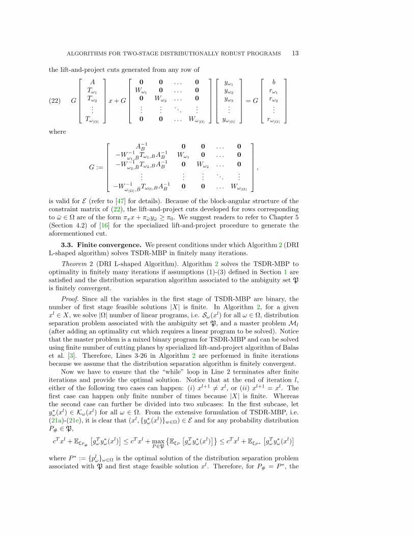
is valid for E (refer to [47] for details). Because of the block-angular structure of theconstraint matrix of (22), the lift-and-project cuts developed for rows correspondingto ω ∈ Ω are of the form πxx+ πωyω ≥ π0. We suggest readers to refer to Chapter 5(Section 4.2) of [16] for the specialized lift-and-project procedure to generate theaforementioned cut.

3.3. Finite convergence. We present conditions under which Algorithm 2 (DRIL-shaped algorithm) solves TSDR-MBP in finitely many iterations.

Theorem 2 (DRI L-shaped Algorithm). Algorithm 2 solves the TSDR-MBP tooptimality in finitely many iterations if assumptions (1)-(3) defined in Section 1 aresatisfied and the distribution separation algorithm associated to the ambiguity set Pis finitely convergent.

Proof. Since all the variables in the first stage of TSDR-MBP are binary, thenumber of first stage feasible solutions |X| is finite. In Algorithm 2, for a givenxl ∈ X, we solve |Ω| number of linear programs, i.e. Sω(xl) for all ω ∈ Ω, distributionseparation problem associated with the ambiguity set P, and a master problem Ml

(after adding an optimality cut which requires a linear program to be solved). Noticethat the master problem is a mixed binary program for TSDR-MBP and can be solvedusing finite number of cutting planes by specialized lift-and-project algorithm of Balaset al. [3]. Therefore, Lines 3-26 in Algorithm 2 are performed in finite iterationsbecause we assume that the distribution separation algorithm is finitely convergent.

Now we have to ensure that the “while” loop in Line 2 terminates after finiteiterations and provide the optimal solution. Notice that at the end of iteration l,either of the following two cases can happen: (i) xl+1 6= xl, or (ii) xl+1 = xl. Thefirst case can happen only finite number of times because |X| is finite. Whereasthe second case can further be divided into two subcases: In the first subcase, lety∗ω(xl) ∈ Kω(xl) for all ω ∈ Ω. From the extensive formulation of TSDR-MBP, i.e.(21a)-(21e), it is clear that (xl, y∗ω(xl)w∈Ω) ∈ E and for any probability distributionP# ∈ P,

cTxl + EξP#

[gTω y

∗ω(xl)

]≤ cTxl + max

P∈P

EξP

[gTω y

∗ω(xl)

]≤ cTxl + EξP∗

[gTω y

∗ω(xl)

]where P ∗ := plωω∈Ω is the optimal solution of the distribution separation problemassociated with P and first stage feasible solution xl. Therefore, for P# = P ∗, the


lower bound LB = cTxl+∑ω∈Ω p

lωg

Tω y∗ω(xl), which is equal to UB . This implies that

(xl, y∗ω(xl)ω∈Ω) is the optimal solution and we get (xl+1, θl+1) = (xl, θl). Hence, inthis subcase the algorithm terminates after returning the optimal solution and optimalobjective value UB .

In the second subcase, let y∗ω(xl) /∈ Kω(xl) for some ω ∈ Ω or more specifically,y∗ω(xl) /∈ 0, 1q1 × Rq−q1 . For this subcase, we derive a lift-and-project cut (Line 9)in (x, yω) subspace to cut-off the point (xl, y∗ω(xl)), project this cutting plane toyω space, add this (globally valid) parametric cut to Sω(x), and resolve the linearprogram for x = xl. Since we assume relatively complete recourse, for each ω ∈ Ω,Kω(xl) and its relaxations are nonempty. Notice that xl ∈ ver(X) where ver(X) isthe set of vertices of conv(X) because X is defined by binary variables only. Hence,x = xl defines a face of conv(E) and since we assume relatively complete recourse,each extreme point of conv(E) ∩ x = xl has yω ∈ 0, 1q1 × Rq−q1 for all ω ∈ Ω.Therefore, using the arguments in the proof of Theorem 3.1 of Balas et al. [3],we can obtain y∗ω(xl) ∈ 0, 1q1 × Rq−q1 , i.e. y∗ω(xl) ∈ Kω(xl), by adding a finitenumber of parametric lift-and-projects cuts to Sω(x). This step can be repeateduntil y∗ω(xl) ∈ Kω(xl) for all ω ∈ Ω. As explained above, under such situation, ouralgorithm terminates and returns the optimal solution after finite number of iterationsas |Ω| is finite and in cases where (xl+1, θl+1) 6= (xl, θl), (xl, θl) will not be visitedagain in future iterations because the optimality cut generated in Line 15 cuts-off thepoint (xl, θl). This completes the proof.

Remark 2. Instead of solving the master problem (11) to optimality at each iter-ation, a branch-and-cut approach can also be adopted for a practical implementation.In this approach, similar to the integer L-shaped method [27], a linear programmingrelaxation of the master problem is solved. The solution thus obtained is used toeither generate a feasibility cut (if this current solution violates any of the relaxedconstraints), or create new branches/nodes following the usual branch-and-cut pro-cedure. The (globally valid) optimality cut, OCS(π∗ω(x), pωω∈Ω), is derived at anode whenever the current solution is also feasible for the original master problem.Interestingly, because of the finiteness of the branch-and-bound approach, it is easyto prove the finite convergence of this algorithm under the conditions mentioned inTheorem 1.

Remark 3. The distribution separation algorithm associated with the momentmatching set PM and Kantorovich set PK are finitely convergent.

3.4. A cutting surface algorithm for TSDR-MBPs. In this section, wepresent a cutting surface algorithm to solve TSDR-MBP where the ambiguity set is aset of finite number distributions (denoted by PF ) which are not known beforehand.This algorithm utilizes branch-and-cut approach to solve master problems, similar tothe integer L-shaped algorithm [27]. Unlike Algorithm 2, we solve the subproblemsto optimality using branch-and-cut method instead of sequentially adding parametriclift-and-project cuts. Furthermore, instead of considering the whole set of distribu-tions PF at once, we solve multiple TSDR-MBPs for an increasing sequence of knownambiguity sets, P0

F , P1F , . . ., such that P0

F ⊂ P1F ⊂ . . . ⊂ PF , until we reach a

subset of PF which contains the optimal probability distribution. Assume that thedistributions in the set Pi

F are known at step i of our implementation. Then, sinceeach probability distribution is equivalent to a set of probabilities of occurrence offinite number of scenarios, i.e. pωω∈Ω, the distribution separation problem (3) as-sociated to the set Pi

F can be solved in finite iterations by explicitly enumerating the


distributions in the set.The cutting surface algorithm works as follows. We start with a known distribu-

tion P0 belonging to PF and set P0F := P0 or obtain it by solving the distribution

separation algorithm corresponding to P for a first stage feasible solution. Then atstep i ≥ 0, given a known ambiguity set Pi

F ⊆ PF , similar to the integer L-shapedmethod, we solve a linear programming relaxation of the master problem. The solu-tion thus obtained is used to either generate a feasibility cut (if this current solutionviolates any of the relaxed constraints), or create new branches/nodes following theusual branch-and-cut procedure. Whenever the current solution is also feasible for theoriginal master problem, we solve the distribution separation problem associated tothe set Pi

F (as mentioned above) to get optimal pωω∈Ω corresponding to the currentfirst stage feasible solution. Thereafter, we derive the globally valid optimality cut,OCS(., pωω∈Ω) and add it to the master problem. We continue the exploration ofthe nodes until we solve the TSDR-MBP for the ambiguity set Pi

F . Then we uti-lize thus obtained optimal solution to solve the distribution separation problem (3)associated to PF and obtain the optimal probability distribution. In case this distri-bution already belongs to Pi

F , we terminate our implementation; otherwise we add itto Pi

F to get Pi+1F and resolve the TSDR-MBP for the ambiguity set Pi+1

F using theaforementioned procedure.

4. Computational experiments. In this section, we evaluate the performanceof the DRI L-shaped algorithm (Algorithm 2) and the cutting surface algorithm (dis-cussed in the previous section) by solving DR versions of stochastic server locationproblem (SSLP), stochastic multiple binary knapsack problem (SMKP), and SSLPwith random recourse (SSLPR). The SSLP and SMKP instances are part of theStochastic Integer Programming Library (SIPLIB) [1], and the SSLPR instances aretaken from [31]. These instances have only binary variables in the first stage andmixed binary programs in the second stage. Also, the probability of occurrence ofeach scenario is same in these instances, i.e. pω = 1/|Ω| for all ω ∈ Ω. On theother hand, in our DR version of SSLP, SMKP, and SSLPR, referred to as the distri-butionally robust server location problem (DRSLP), distributionally robust multiplebinary knapsack problem (DRMKP), DRSLP with random recourse (DRSLPR), re-spectively, the probability distribution belongs to the moment matching set PM (5) orKantorovich set PK (7). Recall that the distribution separation problem associatedto PM and PK are linear programs and both PM and PK are polytopes with finitenumber of extreme points. This implies that in these two cases, the ambiguity setis a set of finite number of distributions corresponding to the extreme points whichare not known beforehand and the associated distribution separation algorithms arefinitely convergent.

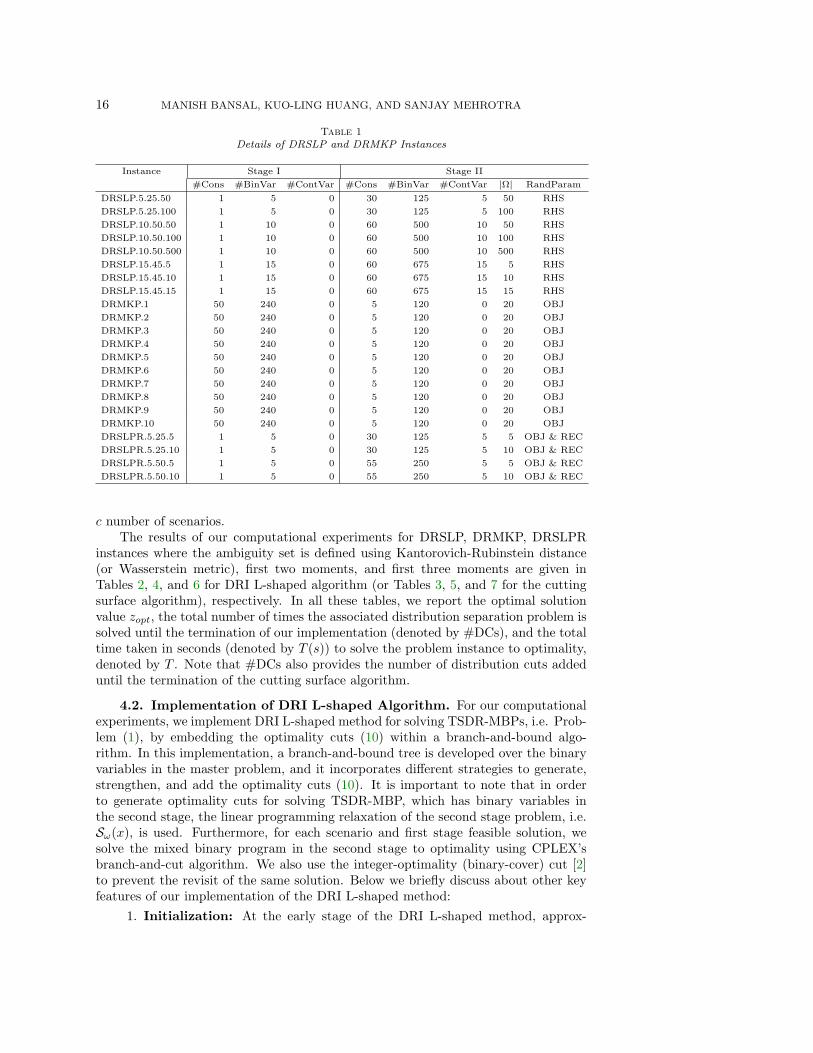
4.1. Instance generation. In Table 1, we provide details of the DRSLP, DRMKP,and DRSLPR instances used for our experiments. In particular, #Cons, #BinVar,and #ContVar denote the number of constraints, binary variables, and continuousvariables, respectively, in Stage I and Stage II of the problems. The number of sce-narios is given by the column labeled as |Ω|. Also, only the right hand side, i.e. rω,are uncertain in DRSLP instances, only the coefficients in the objective function, i.e.gω, are uncertain in DRMKP instances, and both recourse matrix, i.e. Wω, and gωare uncertain in DRSLPR instances. For the sake of uniformity, we are using simi-lar nomenclature for DRSLP and DRSLPR as used for SSLP in SIPLIB [1]. Noticethat instance DRSLP(R).α.β.c has α number of binary variables in the first stage,α × β binary variables and α non-zero continuous variables in the second stage, and


Table 1Details of DRSLP and DRMKP Instances

Instance Stage I Stage II

#Cons #BinVar #ContVar #Cons #BinVar #ContVar |Ω| RandParam

DRSLP.5.25.50 1 5 0 30 125 5 50 RHS

DRSLP.5.25.100 1 5 0 30 125 5 100 RHS

DRSLP.10.50.50 1 10 0 60 500 10 50 RHS

DRSLP.10.50.100 1 10 0 60 500 10 100 RHS

DRSLP.10.50.500 1 10 0 60 500 10 500 RHS

DRSLP.15.45.5 1 15 0 60 675 15 5 RHS

DRSLP.15.45.10 1 15 0 60 675 15 10 RHS

DRSLP.15.45.15 1 15 0 60 675 15 15 RHS

DRMKP.1 50 240 0 5 120 0 20 OBJ

DRMKP.2 50 240 0 5 120 0 20 OBJ

DRMKP.3 50 240 0 5 120 0 20 OBJ

DRMKP.4 50 240 0 5 120 0 20 OBJ

DRMKP.5 50 240 0 5 120 0 20 OBJ

DRMKP.6 50 240 0 5 120 0 20 OBJ

DRMKP.7 50 240 0 5 120 0 20 OBJ

DRMKP.8 50 240 0 5 120 0 20 OBJ

DRMKP.9 50 240 0 5 120 0 20 OBJ

DRMKP.10 50 240 0 5 120 0 20 OBJ

DRSLPR.5.25.5 1 5 0 30 125 5 5 OBJ & REC

DRSLPR.5.25.10 1 5 0 30 125 5 10 OBJ & REC

DRSLPR.5.50.5 1 5 0 55 250 5 5 OBJ & REC

DRSLPR.5.50.10 1 5 0 55 250 5 10 OBJ & REC

c number of scenarios.The results of our computational experiments for DRSLP, DRMKP, DRSLPR

instances where the ambiguity set is defined using Kantorovich-Rubinstein distance(or Wasserstein metric), first two moments, and first three moments are given inTables 2, 4, and 6 for DRI L-shaped algorithm (or Tables 3, 5, and 7 for the cuttingsurface algorithm), respectively. In all these tables, we report the optimal solutionvalue zopt, the total number of times the associated distribution separation problem issolved until the termination of our implementation (denoted by #DCs), and the totaltime taken in seconds (denoted by T (s)) to solve the problem instance to optimality,denoted by T . Note that #DCs also provides the number of distribution cuts addeduntil the termination of the cutting surface algorithm.

4.2. Implementation of DRI L-shaped Algorithm. For our computationalexperiments, we implement DRI L-shaped method for solving TSDR-MBPs, i.e. Prob-lem (1), by embedding the optimality cuts (10) within a branch-and-bound algo-rithm. In this implementation, a branch-and-bound tree is developed over the binaryvariables in the master problem, and it incorporates different strategies to generate,strengthen, and add the optimality cuts (10). It is important to note that in orderto generate optimality cuts for solving TSDR-MBP, which has binary variables inthe second stage, the linear programming relaxation of the second stage problem, i.e.Sω(x), is used. Furthermore, for each scenario and first stage feasible solution, wesolve the mixed binary program in the second stage to optimality using CPLEX’sbranch-and-cut algorithm. We also use the integer-optimality (binary-cover) cut [2]to prevent the revisit of the same solution. Below we briefly discuss about other keyfeatures of our implementation of the DRI L-shaped method:

1. Initialization: At the early stage of the DRI L-shaped method, approx-


Table 2Computational results for the DRI L-shaped algorithm: Ambiguity set is defined using KR distance

Instance ε = 5.0 ε = 10.0

zopt #DCs T (s) zopt #DCs T (s)

DRSLP.5.25.50 14.0 7 2.6 14.0 7 2.5

DRSLP.5.25.100 -40.0 10 7.3 -40.0 10 7.1

DRSLP.10.50.50 -200.0 5 240.0 -200.0 5 236.6

DRSLP.10.50.100 -237.0 16 656.1 -237.0 16 657.2

DRSLP.10.50.500 -159.0 7 1151.6 -159.0 7 1148.9

DRSLP.15.45.5 -252.0 5 288.5 -252.0 5 287.8

DRSLP.15.45.10 -220.0 7 518.4 -220.0 7 515.2

DRSLP.15.45.15 -208.0 11 1203.2 -208.0 11 1202.3

DRMKP.1 9686.0 10 285.4 9686.0 6 101.7

DRMKP.2 9388.0 9 906.0 9388.0 5 591.2

DRMKP.3 8844.0 10 1462.2 8844.0 6 900.5

DRMKP.4 9237.0 23 2695.1 9237.0 14 2485.2

DRMKP.5 10024.0 9 1656.9 10024.0 5 1199.0

DRMKP.6 9515.0 9 257.3 9515.0 5 185.9

DRMKP.7 10003.0 9 434.4 10003.0 5 316.2

DRMKP.8 9427.0 28 4554.3 9427.0 18 3503.7

DRMKP.9 10038.0 10 1090.0 10038.0 6 697.3

DRMKP.10 9082.2 13 4870.0 9082.0 7 3072.8

DRSLPR.5.25.5 -129105.5 55 291.7 -129025.2 56 283.1

DRSLPR.5.25.10 -72721.4 75 1222.4 -72702.2 75 1450.2

DRSLPR.5.50.5 99178.4 200 10800.0 99227.0 128 8560.8

DRSLPR.5.50.10 99734.1 51 10800.0 99929.6 49 10800.0

Table 3Computational results for the cutting surface algorithm: Kantorovich set as the ambiguity set

Instance ε = 5.0 ε = 10.0

zopt #DCs T (s) zopt #DCs T (s)

DRSLP.5.25.50 14.0 5 4.1 14.0 5 4.6

DRSLP.5.25.100 -40.0 7 21.2 -40.0 7 23.4

DRSLP.10.50.50 -200.0 3 136.2 -200.0 3 134.3

DRSLP.10.50.100 -237.0 7 712.9 -237.0 7 710.7

DRSLP.10.50.500 -159.0 3 611.9 -159.0 3 614.0

DRSLP.15.45.5 -252.0 5 182.2 -252.0 5 181.0

DRSLP.15.45.10 -220.0 5 772.5 -220.0 5 773.7

DRSLP.15.45.15 -208.0 4 584.0 -208.0 4 584.7

DRMKP.1 9686.0 10 243.2 9686.0 9 780.0

DRMKP.2 9388.0 10 878.4 9388.0 6 589.6

DRMKP.3 8844.0 11 1345.1 8844.0 11 5685.0

DRMKP.4 9237.0 14 10800.0 9237.0 10 10800.0

DRMKP.5 10024.0 11 3732.5 10024.0 6 1053.8

DRMKP.6 9515.0 10 225.0 9515.0 6 162.6

DRMKP.7 10003.0 10 386.7 10003.0 6 261.9

DRMKP.8 9426.8 18 2910.4 9426.9 11 2301.2

DRMKP.9 10038.0 18 10800.0 10038.0 10 3739.4

DRMKP.10 9084.0 10 10800.0 9084.0 10 10800.0

DRSLPR.5.25.5 -128934.5 130 10800.0 -128660.1 134 10800.0

DRSLPR.5.25.10 -72735.4 34 10800.0 -72701.3 34 10800.0

DRSLPR.5.50.5 99114.9 83 10800.0 99204.2 81 10800.0

DRSLPR.5.50.10 99693.7 26 10800.0 99721.9 26 10800.0

imation of the recourse function tends to be worse because the optimalitycuts (10) are based on a linear programming relaxation of the second stage


problems. As a result, these cuts generated at the early stage may becomeunpromising eventually. To handle this issue, TSDR-LP is solved using theDR L-shaped method and the generated optimality cuts are used to get aninitial approximation for the recourse function. This provides a stronger lowerbound for the branch-and-cut procedure.

2. Hybrid cut method. Each optimality cut corresponds to a scenario, andtherefore, these cuts can be added to the master problem in two differentways: (1) Multi-cut approach, i.e. all optimality cuts are added to the mas-ter problem, and (2) Single-cut approach, i.e. a single cut (10) obtained byaggregating all optimality cut is added to the master problem. A tradeoffsolution between single-cut and multi-cut approaches is called a hybrid-cutapproach, which attempts to find a balance between information loss (due toaggregation) and computing time gains (due to less number of cuts gener-ated) [41, 44]. This method has been incorporated in our implementation.

3. Cut consolidation technique. In order to reduce the size of the mas-ter problem, it may be useful to remove inactive optimality cuts generatedin previous iterations. To do so, a cut consolidation technique of Wolf andKoberstein [44] has been incorporated in our implementation which not onlyremoves the inactive cuts but also generates a new cut by aggregating allinactive cuts generated in the same iteration. This technique preserves infor-mation of the recourse function, and thus potentially avoids recomputing thesame cuts after being removed.

4. Cut reactivation technique. The idea behind the cut reactivation tech-nique is to store the removed cuts (which have been consolidated) in a separatecut pool, and conditionally “reactivate” some of these cuts by adding themback to the master problem, in case they are useful. More precisely, at aniteration, the violation of each cut in the cut pool is evaluated and then cutswith a significant violation are added back to master problem. The masterproblem is reoptimized and this cut reactivation procedure is repeated for apredetermined number of times.

4.3. Computational results for instances with Kantorovich set as theambiguity set. We solve DRSLP, DRMKP, and DRSLPR instances with Kan-torovich set (7) as the ambiguity set and present our computational results in Ta-bles 2 and 3. We consider two different values of ε, i.e. 5.0 and 10.0, and observe thatfor each problem instance, zopt remains same for both values of ε. It is importantto note that the average number of times the distribution separation problem (8) issolved in DRI L-shaped method and cutting surface algorithm are 23 and 20, respec-tively. Interestingly, the DRI L-shaped algorithm solves all DRSLP and DRMKP in-stances to optimality, whereas the cutting surface algorithm failed to solve DRMKP.4,DRMKP.9, and DRMKP.10 to optimality within a time limit of 3 hours. Out of 8DRSLPR instances, DRI L-shaped solved 5 instances in 40 minutes (on average), butthe cutting surface algorithm failed to solve any instance within 3 hours. Moreover,the DRI L-shaped algorithm is on average two times faster than the cutting surfacealgorithm. Also, notice that for DRSLPR instances in Tables 2 and 3, zopt increaseswith increase in ε as the size of the ambiguity set increases with increase in ε. Inother words, the decision maker becomes conservative as the size of the ambiguity setincreases.

4.4. Computational results for instances with moment matching set asthe ambiguity set. In this section, we discuss about our computational results for


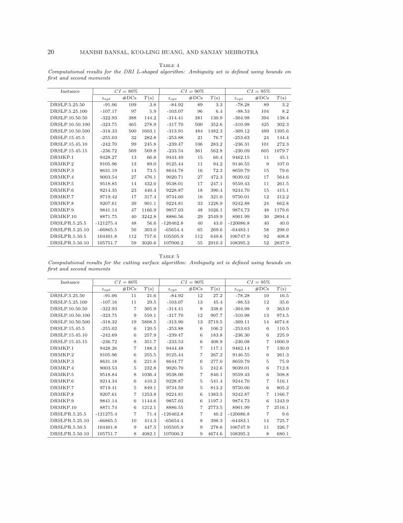
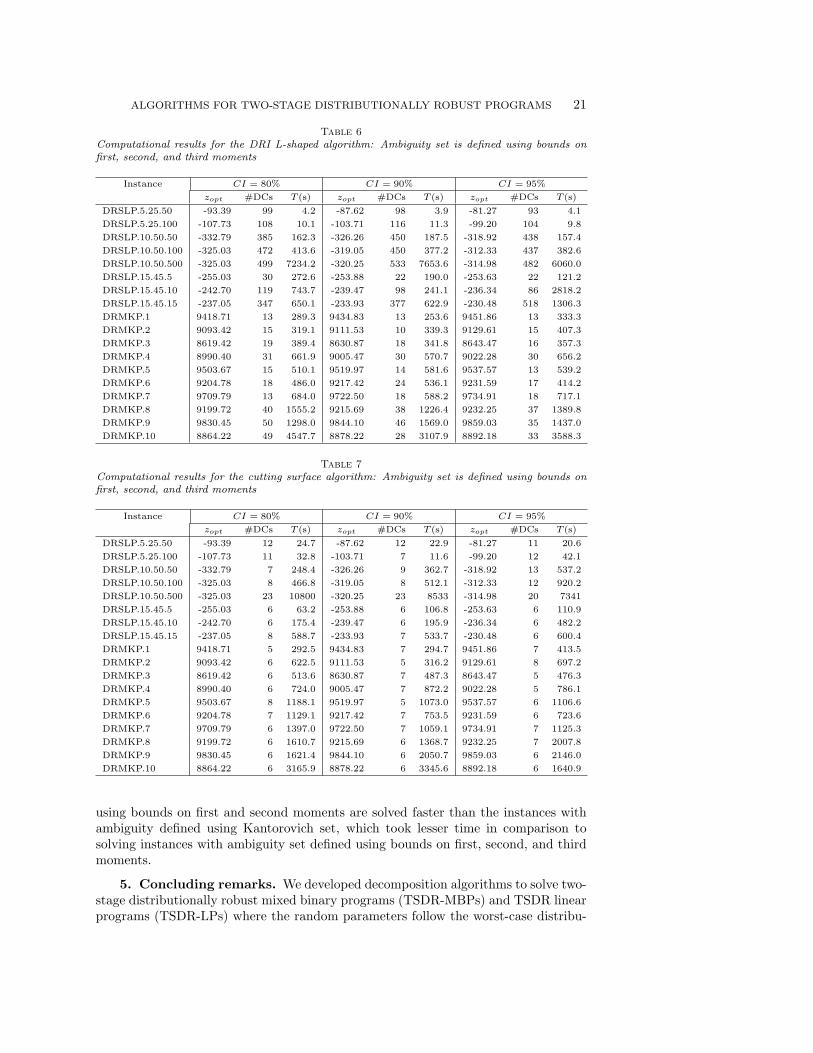
solving DRSLP, DRMKP, and DRSLPR instances with moment matching set (5) asthe ambiguity set. We consider bounds on the first and second moments in Tables4 and 5, and bounds on the first, second, and third moments in Tables 6 and 7.Furthermore, in each of these tables we consider three different values of confidenceinterval (CI), i.e. 80%, 90%, and 95%. Observe that for each problem instance in eachtable, zopt increases with increase in CI as the size of the ambiguity set increases withincrease in CI. In other words, the decision maker becomes conservative as the size ofthe ambiguity set increases. Because of the similar argument, it is evident that thezopt decreases when additional bound constraints are added in the moment matchingset. Comparing zopt for each problem instance with same CI in Tables 4 and 6 (orTables 5 and 7), we notice that zopt decreases because of the presence of bounds onthe third moment.

Next we evaluate the performance of DRI L-shaped algorithm and the cuttingsurface algorithm in solving DRSLP, DRMKP, and DRSLPR instances with momentmatching set. The DRI L-shaped algorithm solves DRSLP and DRMKP instancesto optimality, whereas for instance DRSLP.10.50.500 in Table 7, the cutting surfacealgorithm failed to terminate within the time limit of 3 hours. With regard to theDRSLPR instances, both algorithms solved the instances where ambiguity set is de-fined using bounds on first and second moments (Tables 4 and 5), but both of themfailed to even perform initialization step (discussed in Section 4.2) within 3 hours forthe instances where ambiguity set is defined using bounds on first, second, and thirdmoments. On average DRI L-shaped algorithm is 1.4 times faster than the cuttingsurface algorithm. However, for some instances the latter is faster than the former.In addition, these two algorithms differ in the number of the times distribution sepa-ration problems is solved. As expected #DCs is more for DRI L-shaped algorithm incomparison to the cutting surface algorithm.

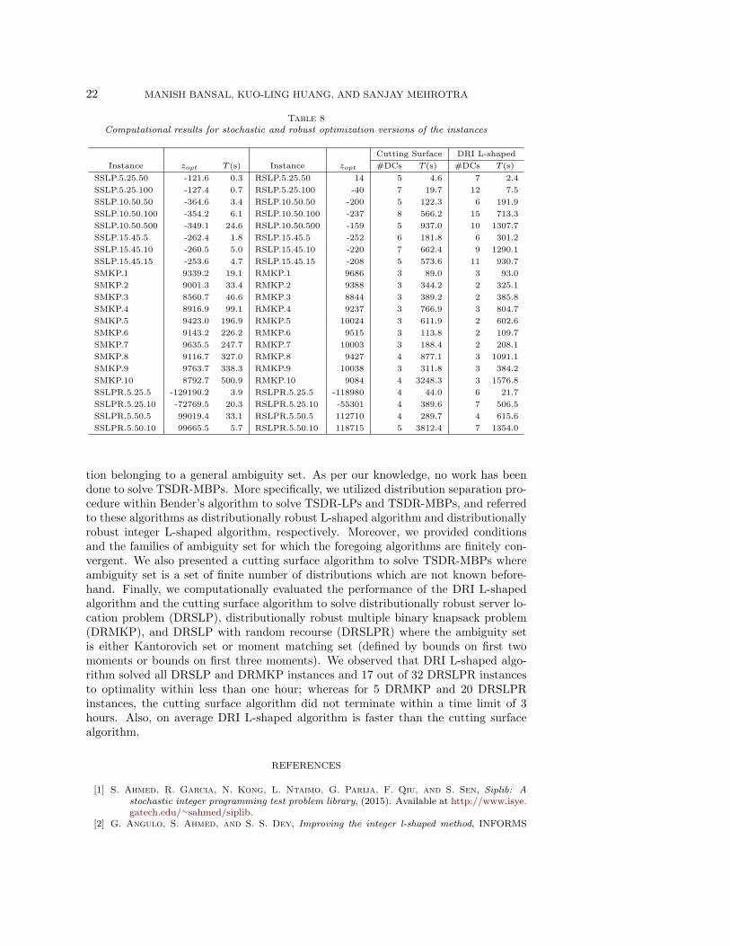
4.5. Computational results for stochastic and robust optimization ver-sions of the test instances. In Table 8, we report the results of computationalexperiments performed on stochastic and robust optimization versions of the DRSLP,DRMKP, and DRSLPR instances. It is important to note that when |P| = 1, the cut-ting surface algorithm and DRI L-shaped algorithm are same as the integer L-shapedalgorithm with the additional features discussed in Section 4.2. For the stochasticversions, we use the same nomenclature as used in the SIPLIB library and [31], i.e.SSLP, SMKP, and SSLPR. We denote the robust optimization versions of the DRSLP,DRMKP, and DRSLPR instances by RSLP, RMKP, and RSLPR, respectively, whichare generated by setting plω∗ = 1 for the scenario ω∗ that has maximum recoursevalue Qω(xl), and use zero probability for the remaining scenarios, i.e. plω = 0 forω ∈ Ω\ω∗.

By observing the optimal objective value zopt of all instances in Tables 2-8, it isclear that the RSLP, RMKP, and RSLPR instances are the most conservative (risk-averse) of all, and the SSLP, SMKP, and SSLPR instances are the risk-neutral in-stances where the probability distribution is known. Whereas, the DRSLP, DRMKP,and DRSLPR instances are the intermediate level models with an adjustable levelof risk-aversion (depending on how ambiguity set is defined). With regard to thecomputational time taken to solve these instances, (on average) the stochastic op-timization instances are solved faster than the robust optimization instances whichtook lesser time in comparison to solving the DRO instances. Even among the DROinstances, because of different levels of complexity of the distributional separation al-gorithm associated with the ambiguity sets, the instances with ambiguity set defined


Table 4Computational results for the DRI L-shaped algorithm: Ambiguity set is defined using bounds onfirst and second moments

Instance CI = 80% CI = 90% CI = 95%

zopt #DCs T (s) zopt #DCs T (s) zopt #DCs T (s)

DRSLP.5.25.50 -91.06 109 3.8 -84.92 89 3.3 -78.28 89 3.2

DRSLP.5.25.100 -107.17 97 5.9 -103.07 96 6.4 -98.53 104 8.2

DRSLP.10.50.50 -322.93 388 144.2 -314.41 381 130.9 -304.98 394 138.4

DRSLP.10.50.100 -323.75 465 278.9 -317.70 500 352.6 -310.98 425 302.3

DRSLP.10.50.500 -318.33 500 1603.1 -313.91 484 1482.3 -309.12 489 1395.6

DRSLP.15.45.5 -255.03 32 282.8 -253.88 21 76.7 -253.63 24 144.4

DRSLP.15.45.10 -242.70 99 245.8 -239.47 106 283.2 -236.31 101 272.3

DRSLP.15.45.15 -236.72 569 569.8 -233.54 361 562.8 -230.09 605 1079.7

DRMKP.1 9428.27 13 66.8 9444.49 15 60.4 9462.15 11 45.1

DRMKP.2 9105.96 13 89.0 9125.44 11 94.2 9146.55 9 107.0

DRMKP.3 8631.19 14 73.5 8644.78 16 72.3 8659.79 15 79.6

DRMKP.4 9003.54 27 476.1 9020.71 27 472.3 9039.02 17 564.6

DRMKP.5 9518.85 14 432.0 9538.01 17 247.1 9559.43 11 261.5

DRMKP.6 9214.35 23 440.4 9228.87 18 390.4 9244.70 15 415.1

DRMKP.7 9719.42 17 317.4 9734.60 16 321.0 9750.01 12 312.2

DRMKP.8 9207.61 39 901.1 9224.81 33 1228.9 9242.88 24 662.8

DRMKP.9 9841.14 47 1166.9 9857.03 48 1026.1 9874.73 48 1179.6

DRMKP.10 8871.75 40 3242.8 8886.56 29 2549.9 8901.99 30 2894.4

DRSLPR.5.25.5 -121275.4 48 56.6 -120462.8 40 43.0 -120086.8 40 40.0

DRSLPR.5.25.10 -66865.5 56 303.0 -65654.4 65 269.6 -64483.1 58 298.0

DRSLPR.5.50.5 104401.8 112 757.6 105505.9 112 649.6 106747.9 92 408.8

DRSLPR.5.50.10 105751.7 59 3020.6 107000.2 55 2910.3 108395.2 52 2837.9

Table 5Computational results for the cutting surface algorithm: Ambiguity set is defined using bounds onfirst and second moments



DRSLP.5.25.50 -91.06 11 21.6 -84.92 12 27.2 -78.28 10 16.5

DRSLP.5.25.100 -107.16 11 29.5 -103.07 13 45.4 -98.53 12 35.6

DRSLP.10.50.50 -322.93 7 305.9 -314.41 8 338.6 -304.98 9 363.0

DRSLP.10.50.100 -323.75 9 559.1 -317.70 12 907.7 -310.98 13 974.5

DRSLP.10.50.500 -318.32 19 5808.5 -313.90 13 3719.5 -309.11 14 4074.8

DRSLP.15.45.5 -255.02 6 120.5 -253.88 6 106.2 -253.63 6 110.5

DRSLP.15.45.10 -242.69 6 257.9 -239.47 6 183.8 -236.30 6 225.9

DRSLP.15.45.15 -236.72 8 351.7 -233.53 6 408.9 -230.08 7 1000.9

DRMKP.1 9428.26 7 188.3 9444.48 7 117.1 9462.14 7 130.0

DRMKP.2 9105.96 6 255.5 9125.44 7 267.2 9146.55 6 261.3

DRMKP.3 8631.18 6 221.6 8644.77 6 277.0 8659.79 5 75.9

DRMKP.4 9003.53 5 232.8 9020.70 5 242.6 9039.01 6 712.8

DRMKP.5 9518.84 8 1036.4 9538.00 7 840.1 9559.43 6 508.8

DRMKP.6 9214.34 6 410.2 9228.87 5 541.4 9244.70 7 516.1

DRMKP.7 9719.41 5 849.1 9734.59 5 813.2 9750.00 6 805.2

DRMKP.8 9207.61 7 1253.8 9224.81 6 1383.5 9242.87 7 1166.7

DRMKP.9 9841.14 6 1144.6 9857.03 6 1197.1 9874.73 6 1243.9

DRMKP.10 8871.74 6 1212.1 8886.55 7 2773.5 8901.99 7 2516.1

DRSLPR.5.25.5 -121275.4 7 71.4 -120462.8 7 40.2 -120086.8 7 9.6

DRSLPR.5.25.10 -66865.5 10 414.3 -65654.4 8 398.3 -64483.1 14 725.7

DRSLPR.5.50.5 104401.8 9 447.5 105505.9 9 278.6 106747.9 11 326.7

DRSLPR.5.50.10 105751.7 8 4082.1 107000.2 9 4674.6 108395.2 8 680.1


Table 6Computational results for the DRI L-shaped algorithm: Ambiguity set is defined using bounds onfirst, second, and third moments



DRSLP.5.25.50 -93.39 99 4.2 -87.62 98 3.9 -81.27 93 4.1

DRSLP.5.25.100 -107.73 108 10.1 -103.71 116 11.3 -99.20 104 9.8

DRSLP.10.50.50 -332.79 385 162.3 -326.26 450 187.5 -318.92 438 157.4

DRSLP.10.50.100 -325.03 472 413.6 -319.05 450 377.2 -312.33 437 382.6

DRSLP.10.50.500 -325.03 499 7234.2 -320.25 533 7653.6 -314.98 482 6060.0

DRSLP.15.45.5 -255.03 30 272.6 -253.88 22 190.0 -253.63 22 121.2

DRSLP.15.45.10 -242.70 119 743.7 -239.47 98 241.1 -236.34 86 2818.2

DRSLP.15.45.15 -237.05 347 650.1 -233.93 377 622.9 -230.48 518 1306.3

DRMKP.1 9418.71 13 289.3 9434.83 13 253.6 9451.86 13 333.3

DRMKP.2 9093.42 15 319.1 9111.53 10 339.3 9129.61 15 407.3

DRMKP.3 8619.42 19 389.4 8630.87 18 341.8 8643.47 16 357.3

DRMKP.4 8990.40 31 661.9 9005.47 30 570.7 9022.28 30 656.2

DRMKP.5 9503.67 15 510.1 9519.97 14 581.6 9537.57 13 539.2

DRMKP.6 9204.78 18 486.0 9217.42 24 536.1 9231.59 17 414.2

DRMKP.7 9709.79 13 684.0 9722.50 18 588.2 9734.91 18 717.1

DRMKP.8 9199.72 40 1555.2 9215.69 38 1226.4 9232.25 37 1389.8

DRMKP.9 9830.45 50 1298.0 9844.10 46 1569.0 9859.03 35 1437.0

DRMKP.10 8864.22 49 4547.7 8878.22 28 3107.9 8892.18 33 3588.3

Table 7Computational results for the cutting surface algorithm: Ambiguity set is defined using bounds onfirst, second, and third moments



DRSLP.5.25.50 -93.39 12 24.7 -87.62 12 22.9 -81.27 11 20.6

DRSLP.5.25.100 -107.73 11 32.8 -103.71 7 11.6 -99.20 12 42.1

DRSLP.10.50.50 -332.79 7 248.4 -326.26 9 362.7 -318.92 13 537.2

DRSLP.10.50.100 -325.03 8 466.8 -319.05 8 512.1 -312.33 12 920.2

DRSLP.10.50.500 -325.03 23 10800 -320.25 23 8533 -314.98 20 7341

DRSLP.15.45.5 -255.03 6 63.2 -253.88 6 106.8 -253.63 6 110.9

DRSLP.15.45.10 -242.70 6 175.4 -239.47 6 195.9 -236.34 6 482.2

DRSLP.15.45.15 -237.05 8 588.7 -233.93 7 533.7 -230.48 6 600.4

DRMKP.1 9418.71 5 292.5 9434.83 7 294.7 9451.86 7 413.5

DRMKP.2 9093.42 6 622.5 9111.53 5 316.2 9129.61 8 697.2

DRMKP.3 8619.42 6 513.6 8630.87 7 487.3 8643.47 5 476.3

DRMKP.4 8990.40 6 724.0 9005.47 7 872.2 9022.28 5 786.1

DRMKP.5 9503.67 8 1188.1 9519.97 5 1073.0 9537.57 6 1106.6

DRMKP.6 9204.78 7 1129.1 9217.42 7 753.5 9231.59 6 723.6

DRMKP.7 9709.79 6 1397.0 9722.50 7 1059.1 9734.91 7 1125.3

DRMKP.8 9199.72 6 1610.7 9215.69 6 1368.7 9232.25 7 2007.8

DRMKP.9 9830.45 6 1621.4 9844.10 6 2050.7 9859.03 6 2146.0

DRMKP.10 8864.22 6 3165.9 8878.22 6 3345.6 8892.18 6 1640.9

using bounds on first and second moments are solved faster than the instances withambiguity defined using Kantorovich set, which took lesser time in comparison tosolving instances with ambiguity set defined using bounds on first, second, and thirdmoments.

5. Concluding remarks. We developed decomposition algorithms to solve two-stage distributionally robust mixed binary programs (TSDR-MBPs) and TSDR linearprograms (TSDR-LPs) where the random parameters follow the worst-case distribu-


Table 8Computational results for stochastic and robust optimization versions of the instances

Cutting Surface DRI L-shaped

Instance zopt T (s) Instance zopt #DCs T (s) #DCs T (s)

SSLP.5.25.50 -121.6 0.3 RSLP.5.25.50 14 5 4.6 7 2.4

SSLP.5.25.100 -127.4 0.7 RSLP.5.25.100 -40 7 19.7 12 7.5

SSLP.10.50.50 -364.6 3.4 RSLP.10.50.50 -200 5 122.3 6 191.9

SSLP.10.50.100 -354.2 6.1 RSLP.10.50.100 -237 8 566.2 15 713.3

SSLP.10.50.500 -349.1 24.6 RSLP.10.50.500 -159 5 937.0 10 1307.7

SSLP.15.45.5 -262.4 1.8 RSLP.15.45.5 -252 6 181.8 6 301.2

SSLP.15.45.10 -260.5 5.0 RSLP.15.45.10 -220 7 662.4 9 1290.1

SSLP.15.45.15 -253.6 4.7 RSLP.15.45.15 -208 5 573.6 11 930.7

SMKP.1 9339.2 19.1 RMKP.1 9686 3 89.0 3 93.0

SMKP.2 9001.3 33.4 RMKP.2 9388 3 344.2 2 325.1

SMKP.3 8560.7 46.6 RMKP.3 8844 3 389.2 2 385.8

SMKP.4 8916.9 99.1 RMKP.4 9237 3 766.9 3 804.7

SMKP.5 9423.0 196.9 RMKP.5 10024 3 611.9 2 602.6

SMKP.6 9143.2 226.2 RMKP.6 9515 3 113.8 2 109.7

SMKP.7 9635.5 247.7 RMKP.7 10003 3 188.4 2 208.1

SMKP.8 9116.7 327.0 RMKP.8 9427 4 877.1 3 1091.1

SMKP.9 9763.7 338.3 RMKP.9 10038 3 311.8 3 384.2

SMKP.10 8792.7 500.9 RMKP.10 9084 4 3248.3 3 1576.8

SSLPR.5.25.5 -129190.2 3.9 RSLPR.5.25.5 -118980 4 44.0 6 21.7

SSLPR.5.25.10 -72769.5 20.3 RSLPR.5.25.10 -55301 4 389.6 7 506.5

SSLPR.5.50.5 99019.4 33.1 RSLPR.5.50.5 112710 4 289.7 4 615.6

SSLPR.5.50.10 99665.5 5.7 RSLPR.5.50.10 118715 5 3812.4 7 1354.0

tion belonging to a general ambiguity set. As per our knowledge, no work has beendone to solve TSDR-MBPs. More specifically, we utilized distribution separation pro-cedure within Bender’s algorithm to solve TSDR-LPs and TSDR-MBPs, and referredto these algorithms as distributionally robust L-shaped algorithm and distributionallyrobust integer L-shaped algorithm, respectively. Moreover, we provided conditionsand the families of ambiguity set for which the foregoing algorithms are finitely con-vergent. We also presented a cutting surface algorithm to solve TSDR-MBPs whereambiguity set is a set of finite number of distributions which are not known before-hand. Finally, we computationally evaluated the performance of the DRI L-shapedalgorithm and the cutting surface algorithm to solve distributionally robust server lo-cation problem (DRSLP), distributionally robust multiple binary knapsack problem(DRMKP), and DRSLP with random recourse (DRSLPR) where the ambiguity setis either Kantorovich set or moment matching set (defined by bounds on first twomoments or bounds on first three moments). We observed that DRI L-shaped algo-rithm solved all DRSLP and DRMKP instances and 17 out of 32 DRSLPR instancesto optimality within less than one hour; whereas for 5 DRMKP and 20 DRSLPRinstances, the cutting surface algorithm did not terminate within a time limit of 3hours. Also, on average DRI L-shaped algorithm is faster than the cutting surfacealgorithm.

REFERENCES

[1] S. Ahmed, R. Garcia, N. Kong, L. Ntaimo, G. Parija, F. Qiu, and S. Sen, Siplib: Astochastic integer programming test problem library, (2015). Available at http://www.isye.gatech.edu/∼sahmed/siplib.

[2] G. Angulo, S. Ahmed, and S. S. Dey, Improving the integer l-shaped method, INFORMS

http://www.isye.gatech.edu/~sahmed/siplib

http://www.isye.gatech.edu/~sahmed/siplib


Journal on Computing, 28 (2016), pp. 483–499.[3] E. Balas, S. Ceria, and G. Cornujols, A lift-and-project cutting plane algorithm for mixed

0-1 programs, Mathematical Programming, 58 (1993), pp. 295–324.[4] M. Bansal, K.-L. Huang, and S. Mehrotra, Tight second-stage formulations in two-stage

stochastic mixed integer programs, SIAM Journal on Optimization, 28(1) (2018), pp. 788–819.

[5] M. Bansal and K. Kianfar, n-step cycle inequalities: facets for continuous multi-mixing setand strong cuts for multi-module capacitated lot-sizing problem, Mathematical Program-ming, (2015), pp. 1–32.

[6] M. Bansal and K. Kianfar, Facets for continuous multi-mixing set with general coefficientsand bounded integer variables, Discrete Optimization, 25 (2017), pp. 1–26.

[7] A. Ben-Tal, D. den Hertog, A. De Waegenaere, B. Melenberg, and G. Rennen, Ro-bust Solutions of Optimization Problems Affected by Uncertain Probabilities, ManagementScience, 59 (2012), pp. 341–357.

[8] A. Ben-Tal and E. Hochman, More Bounds on the Expectation of a Convex Function of aRandom Variable, Journal of Applied Probability, 9 (1972), pp. 803–812.

[9] A. Ben-Tal and E. Hochman, Stochastic Programs with Incomplete Information, OperationsResearch, 24 (1976), pp. 336–347.

[10] J. F. Benders, Partitioning procedures for solving mixed-variables programming problems,Numerische Mathematik, 4 (1962), pp. 238–252.

[11] D. Bertsimas, X. V. Doan, K. Natarajan, and C.-P. Teo, Models for minimax stochasticlinear optimization problems with risk aversion, Mathematics of Operations Research, 35(2010), pp. 580–602.

[12] D. Bertsimas and I. Popescu, Optimal inequalities in probability theory: A convex optimiza-tion approach, SIAM Journal on Optimization, 15 (2005), pp. 780–804.

[13] J. R. Birge and R. J.-B. Wets, Designing approximation schemes for stochastic optimizationproblems, in particular for stochastic programs with recourse, in Stochastic Programming84 Part I, Mathematical Programming Studies, Springer, Berlin, Heidelberg, 1986, pp. 54–102.

[14] G. Calafiore, Ambiguous Risk Measures and Optimal Robust Portfolios, SIAM Journal onOptimization, 18 (2007), pp. 853–877.

[15] C. C. Carøe and J. Tind, A cutting-plane approach to mixed 0–1 stochastic integer programs,European Journal of Operational Research, 101 (1997), pp. 306–316.

[16] M. Conforti, G. Cornujols, and G. Zambelli, Integer Programming, vol. 271 of GraduateTexts in Mathematics, Springer International Publishing, Cham, 2014.

[17] E. Delage and Y. Ye, Distributionally robust optimization under moment uncertainty withapplication to data-driven problems, Operations Research, 58 (2010), pp. 595–612.

[18] J. Dupacova, The minimax approach to stochastic programming and an illustrative applica-tion, Stochastics, 20 (1987), pp. 73–88.

[19] M. Dyer and L. Stougie, Computational complexity of stochastic programming problems,Mathematical Programming, 106 (2006), pp. 423–432.

[20] E. Erdogan and G. Iyengar, Ambiguous chance constrained problems and robust optimiza-tion, Mathematical Programming, 107 (2006), pp. 37–61.

[21] D. Gade, S. Kucukyavuz, and S. Sen, Decomposition algorithms with parametric gomory cutsfor two-stage stochastic integer programs, Mathematical Programming, (2012), pp. 1–26.

[22] G. A. Hanasusanto and D. Kuhn, Conic programming reformulations of two-stage distribu-tionally robust linear programs over wasserstein balls, under review (2016). Available athttps://arxiv.org/abs/1609.07505.

[23] G. A. Hanasusanto, V. Roitch, D. Kuhn, and W. Wiesemann, A distributionally robust per-spective on uncertainty quantification and chance constrained programming, MathematicalProgramming, 151 (2015), pp. 35–62.

[24] C. C. Huang, W. T. Ziemba, and A. Ben-Tal, Bounds on the Expectation of a Convex Func-tion of a Random Variable: With Applications to Stochastic Programming, OperationsResearch, 25 (1977), pp. 315–325.

[25] R. Jiang and Y. Guan, Risk-averse two-stage stochastic program with distributional ambiguity,(2015). Available at http://www.optimization-online.org/DB FILE/2015/05/4908.pdf.

[26] S. Kucukyavuz and S. Sen, An introduction to two-stage stochastic mixed-integer program-ming, in The Operations Research Revolution (INFORMS Tutorials in Operations Re-search, 2017, ch. 1, pp. 1–27, https://doi.org/10.1287/educ.2017.0171.

[27] G. Laporte and F. V. Louveaux, The integer L-shaped method for stochastic integer programswith complete recourse, Operations Research Letters, 13 (1993), pp. 133–142.

[28] D. K. Love and G. Bayraksan, Phi-divergence constrained ambiguous stochastic pro-

https://arxiv.org/abs/1609.07505

http://www.optimization-online.org/DB_FILE/2015/05/4908.pdf

https://doi.org/10.1287/educ.2017.0171


grams for data-driven optimization, under review (2016). Available at http://www.optimization-online.org/DB HTML/2016/03/5350.html.

[29] S. Mehrotra and D. Papp, A cutting surface algorithm for semi-infinite convex programmingwith an application to moment robust optimization, SIAM J. on Optimization, 24 (2014),pp. 1670–1697.

[30] S. Mehrotra and H. Zhang, Models and algorithms for distributionally robust least squaresproblems, Mathematical Programming, 148 (2014), pp. 123–141.

[31] L. Ntaimo, Disjunctive decomposition for two-stage stochastic mixed-binary programs withrandom recourse, Operations Research, 58 (2009), pp. 229–243.

[32] G. Pflug, A. Pichlera, and D. Wozabalb, The 1/n investment strategy is optimal underhigh model ambiguity, Journal of Banking and Finance, 36 (2012), pp. 410–417.

[33] G. Pflug and D. Wozabal, Ambiguity in portfolio selection, Quantitative Finance, 7 (2007),pp. 435–442,.

[34] K. Postek, A. Ben-Tal, D. den Hertog, and B. Melenberg, Exact Robust Counterparts ofAmbiguous Stochastic Constraints Under Mean and Dispersion Information, OperationsResearch, in print (2018).

[35] A. Prekopa, Stochastic Programming, Kluwer Academic, 1995.[36] H. Scarf, A min-max solution of an inventory problem, in Studies in the Mathematical Theory

of Inventory and Production, 1958, ch. 12, pp. 201–209.[37] S. Sen and J. L. Higle, The C3 theorem and a D2 algorithm for large scale stochastic mixed-

integer programming: set convexification, Mathematical Programming, 104 (2005), pp. 1–20.

[38] A. Shapiro and S. Ahmed, On a class of minimax stochastic programs, SIAM Journal onOptimization, 14 (2004), pp. 1237–1249.

[39] A. Shapiro and A. Kleywegt, Minimax analysis of stochastic problems, Optimization Meth-ods and Software, 17 (2002), pp. 523–542.

[40] H. D. Sherali and B. M. Fraticelli, A modification of benders’ decomposition algorithm fordiscrete subproblems: An approach for stochastic programs with integer recourse, Journalof Global Optimization, 22 (2002), pp. 319–342.

[41] S. Trukhanov, L. Ntaimo, and A. Schaefer, Adaptive multicut aggregation for two-stagestochastic linear programs with recourse, European Journal of Operational Research, 206(2010), pp. 395 – 406.

[42] R. Van Slyke and R. Wets, L-shaped linear programs with applications to optimal control andstochastic programming, SIAM Journal on Applied Mathematics, 17 (1969), pp. 638–663.

[43] Z. Wang, P. W. Glynn, and Y. Ye, Likelihood robust optimization for data-driven problems,Computational Management Science, 13 (2016), pp. 241–261.

[44] C. Wolf and A. Koberstein, Dynamic sequencing and cut consolidation for the parallelhybrid-cut nested l-shaped method, European Journal of Operational Research, 230 (2013),pp. 143 – 156.

[45] D. Wozabal, A framework for optimization under ambiguity, Annals of Operations Research,193 (2012), pp. 21–47.

[46] h. Yankolu and D. den Hertog, Safe Approximations of Ambiguous Chance ConstraintsUsing Historical Data, INFORMS Journal on Computing, 25 (2012), pp. 666–681.

[47] M. Zhang and S. Kucukyavuz, Finitely convergent decomposition algorithms for two-stagestochastic pure integer programs, SIAM Journal on Optimization, 24 (2014), pp. 1933–1951.

[48] C. Zhao and Y. Guan, Data-driven risk-averse two-stage stochastic program with ζ-structureprobability metrics, under review (2015). Available at http://www.optimization-online.org/DB HTML/2015/07/5014.html.

http://www.optimization-online.org/DB_HTML/2016/03/5350.html




decomposition algorithms for two-stage …

Documents