Decomposing the Persistence of Real Exchange Rates

Dimitrios Malliaropulos∗ Ekaterini Panopoulou†

Theologos Pantelidis‡ Nikitas Pittis§

Abstract

We propose a new methodology for decomposing the persistence of deviations

from Purchasing Power Parity (PPP). By directly comparing the impulse response

function (IRF) of a VAR model, where the real exchange rate is Granger caused by a

set of candidate variables, with the IRF of the equivalent ARMA model for the real

exchange rate, we capture the effects of the Granger-causing variables on the half-life

of deviations from PPP. Our empirical results for a set of 20 industrialised countries

suggest that up to 62% of the persistence of real exchange rates can be attributed

to interest rate differentials and relative business cycle position with the numenaire

country.

Keywords: real exchange rate; persistence measures; VAR; impulse response func-

tion; PPP.

JEL Classification: F31, C32.

Acknowledgements: Financial support from the Greek Ministry of Education

and the European Union under “Hrakleitos” grant is greatly appreciated. Panopoulou

thanks the Irish Higher Education Authority for providing research support under the

North South Programme for Collaborative Research. The usual disclaimer applies.

∗Department of Banking and Financial Management, University of Piraeus and EFG-Eurobank.†Department of Statistics and Insurance Science, University of Piraeus, Greece and Department of Eco-

nomics, National University of Ireland, Maynooth. Correspondence to: Ekaterini Panopoulou, Departmentof Statistics and Insurance Science, University of Piraeus, 80 Karaoli & Dimitriou Str., 18534, Piraeus,Greece. E-mail: apano@unipi.gr. Tel: 0030 210 4142728. Fax: 0030 210 4142340.

‡Department of Economics, National University of Ireland, Maynooth.§Department of Banking and Financial Management, University of Piraeus.

1

1 Introduction

Long-run Purchasing Power Parity (PPP) states that real exchange rates, defined as the

relative price of a basket of goods expressed in a common currency, should be stationary,

implying that changes in the real exchange rate should be arbitraged away in the long run.

Yet, one characteristic of real exchange rates is that they are highly persistent processes.

In other words, the speed at which a given shock to the real exchange rate dissipates

is very slow. One measure of persistence is half-life, defined as the number of periods

required for a given shock to reduce to half its initial value. A large number of empirical

studies has found that real exchange rates are stationary, but highly persistent processes

with the consensus of half-lives of deviations from PPP between three and five years as

Rogoff (1996) claimed.1

The majority of empirical studies compute half-lives of PPP deviations within a uni-

variate framework, typically by estimating a first-order autoregressive model (AR(1)).2

In such a specification, the error term, which accounts for the variation of the real ex-

change rate, can be thought of as a ‘composite shock’ that incorporates various individual

shocks, such as monetary shocks or shocks to tastes and technology. As a result, impulse

response analysis within the univariate framework cannot identify the effect of each indi-

vidual shock, but simply tells us how fast the real exchange rate adjusts to a disturbance

of unknown origins.

Various studies have attempted to measure the contributions of monetary and real

shocks to the variability of the real exchange rate by estimating structural Vector Autore-

gressive (VAR) models. The results are mixed. Clarida and Gali (1994) find monetary

shocks to be unimportant in contrast to aggregate demand shocks, which appear to be the

major determinant of real exchange rate variability. On the other hand, Rogers (1999) re-

ports that 20% to 60% of the variability of real exchange rates is attributable to monetary

shocks.1Taylor (2003, 2006) and Taylor and Taylor (2004) provide us with excellent literature reviews on the

issue.2Alternative methodologies include panel data models (see, inter alia, Frankel and Rose, 1996; Lothian,

1997; and Papell,1997) and nonlinear time series models (see, Taylor and Peel, 2000; Shintani, 2006; amongothers).

2

In this paper, we also employ a VAR methodology, although we take a different ap-

proach than decomposing the variance of the real exchange rate within a structural VAR

framework. Rather than trying to identify the sources of structural shocks to the real

exchange rate, we measure the relative contribution of a number of explanatory variables

to the persistence of a shock on the real exchange rate by comparing the half-life estimates

obtained from a VAR model with those obtained from the equivalent univariate ARMA

models of the real exchange rate.3 The VAR model includes apart from the real exchange

rate, a set of explanatory variables that determine the short-run dynamics of the real ex-

change rate. By doing so, we are able to isolate the effect of these explanatory variables on

the speed of adjustment of the real exchange rate towards the PPP level. By comparing

the half-life of the VAR model with the half-life of the equivalent univariate model, we are

able to measure directly the contribution of the explanatory variables to the persistence of

the real exchange rate. For example, if the multivariate half-life estimates are not shorter

than the univariate ones, then the explanatory variables cannot account, even partly, for

the persistence of a shock on the real exchange rate.

In order to motivate our proposed methodology, let us first define the real exchange

rate, y1t, as the relative price of foreign goods in terms of domestic goods. In log form:

y1t ≡ st − (pt − p∗t )

where st is the nominal exchange rate, measured in units of domestic currency per unit of

foreign currency, and pt (p∗t ) is the domestic (foreign) price index. Furthermore, let Yt =

[y1t,y2t]0 be an (n×1)−vector of variables where y2t is an (n−1)-vector of macroeconomic

variables, which affect the dynamic adjustment of the real exchange rate towards the PPP

level.

Let us further assume that Yt follows a n−variate VAR(1) model.4 It is well knownthat each variable in the VAR(1) model (including y1t) has an equivalent univariate

3The methodology introduced in this paper can be used to measure the contribution of any (group of)explanatory variable(s) to the persistence of any variable of interest.

4The VAR(1) model is assumed at this stage for expositional purposes only. This assumption is relaxedin Section 2 that describes the methodology in a general framework.

3

ARMA(n, n − 1) representation, where n and n − 1 are the maximum orders of the au-

toregressive and moving average parts, respectively (see Lutkepohl, 1993). In view of this

‘equivalence’, there is no specification error involved in one’s decision to employ the ARMA

model for estimating the response of y1t to a unit shock in the error term, say et. The

latter, however, is a combination of the errors in the VAR model, which in turn implies

that the origins of this shock cannot be identified. Assume for simplicity that there is

no contemporaneous correlation among the elements of Yt, and consider the first equation

of the VAR model, that is the one for the real exchange rate.5 The error term in this

equation, say ε1t, describes the shocks in y1t not accounted for by y2t, that is it describes

the effects of any other random factors that affect y1t. The VAR-response, IRFm, of y1t to

a unit shock in ε1t will, in general, be different from its equivalent ARMA-response, IRFu,

to a unit shock in et if the variables y2t have actually a role to play. Indeed, the difference,

D = IRFu − IRFm, describes the dynamic adjustment path of the real exchange rate

which is solely due to the observed variables y2t. Obviously, the effects of other factors

that influence y1t not taken into account in the VAR specification are captured by IRFu

itself. The bigger D is, the more (less) important the role of y2t (other factors) for the

persistence of the y1t will be.

To further clarify our point, assume that the half-life of y1t, estimated within the

ARMA model for y1t is 20 quarters. On the other hand, assume that the half-life estimate

obtained from the VAR model, which includes y1t and y2t is only 12 quarters. This means

that the contribution of y2t to the half-life of y1t is 20-12=8 quarters. The remaining 12

quarters is the number of periods required for y1t to adjust (by half) to shocks in other

factors. In such a scenario, y2t accounts for 40% (=8/20) of the persistence of y1t.

Our methodology has three main advantages over the structural VAR approaches pre-

viously employed in the literature. First, it does not require to impose identifying restric-

tions in order to decompose innovations in the real exchange rate into structural shocks.

Second, it allows to recover directly the effect of any variable on the persistence of PPP de-

viations from the impulse-response function, as opposed to the structural VAR approach,

5Once again, we consider the first equation of the VAR model for expositional purposes only. Thisassumption is relaxed in Section 2.

4

which focuses on the effect of some type of structural shocks on the variance of the real

exchange rate. Third, it provides simple testable conditions on the estimates of the VAR

which allow the researcher to assess the role of any candidate variable in determining the

persistence of PPP deviations.

Our aim is to shed some light on the contribution of a set of macroeconomic vari-

ables, which are considered to be fundamental determinants of real exchange rates, to the

persistence of deviations from PPP. This set of variables includes output growth differen-

tials, short- and long-term interest rate differentials (both nominal and real) between the

domestic and the foreign economy.

The remainder of the paper is structured as follows. Section 2 describes the method-

ology introduced in this paper and presents our main theoretical results. In Section 3 we

provide an empirical illustration of our methodology by quantifying the relative impor-

tance of a set of macroeconomic variables on the persistence of the real exchange rate.

Finally, Section 4 concludes this paper.

2 Impulse Response Analysis: MultivariateModels and their

Equivalent Univariate Representations

This section highlights our methodology that aims at measuring the contribution of a

group of explanatory variables to the persistence of a variable of interest. The method-

ology is based on the fact that the impulse response analysis within a VAR model differs

in general from that conducted within the equivalent univariate ARMA models. The dif-

ference between the two IRFs reveals the contribution of the explanatory variables to the

persistence of a shock on the variable of interest.

The analysis is based on a zero-mean, n−variate VAR(p) model.6 Throughout this sec-tion, we assume that we want to measure the contribution of zt := (y1t, .., yk−1t, yk+1t, .., ynt)0

to the persistence of ykt.7 Thoughout this section, the subscript k is assumed to be fixed.

6The existence of a non-zero mean does not affect the impulse response analysis.7 In the empirical part of the paper (Section 3) ykt stands for the real exchange rate.

5

Let Yt = (y1t, y2t, .., ynt)0 follow a stable VAR(p) process:

Yt = A1Yt−1 +A2Yt−2 + ..+ApYt−p + Ut (1)

where Am := [aij,m], i, j = 1, 2, .., n and m = 1, 2, .., p are (n× n) matrices of parameters.

The error vector Ut = (u1t, u2t, .., unt)0 is a white noise process, that is, E(Ut) = 0,

E(UtU0t) = Σu := [σij ], i, j = 1, 2, .., n and E(UtU

0s) = 0 for t 6= s. The covariance matrix

Σu is assumed to be non-singular.

Before we proceed any further, it is important to emphasize the role of σik, i 6= k on

the interpretation of the errors in the VAR model. If σik 6= 0 for some i 6= k, then the error,

ukt, in the k − th equation of the VAR model, cannot be interpreted as the innovations

driving ykt. On the other hand, if σik = 0 for every i 6= k, then ukt regains its status

as ‘the innovations’ of ykt in the VAR model and can be thought of as summarizing the

factors that contribute to the variability of ykt, other than ykt−i and zt−i, i = 1, 2, .., p.

Following Lutkepohl (1993), each component series yit, i = 1, 2, .., n of Yt has an

equivalent univariate ARMA(p, q) representation where p ≤ np and q ≤ (n − 1)p.8 Forexample, the equivalent univariate model for ykt is:

ykt = a1,kykt−1 + ...+ ap,kykt−p + ekt + γ1,kekt−1 + ..+ γq,kekt−q (2)

where ai,k, i = 1, 2, .., p and γi,k, i = 1, 2, .., q are functions of the VAR parameters aij,m

and σij ( i, j = 1, 2, .., n and m = 1, 2, .., p). In view of this ‘equivalence’, there is no

specification error involved in one’s decision to employ the ARMA model for estimating

the response of ykt to a unit shock in the error term ekt.

It is interesting to note that the MA error term, wkt ≡ ekt + γ1,kekt−1 + ..+ γq,kekt−q,

is related to the original VAR error. The error in the univariate representation of ykt can

be thought of as an aggregation of the original errors in the VAR model. As a result, the

variation of wkt is due to the variation of any conbination of uit, i = 1, 2, ..., n. Furthermore,

the variance, σ2k, of the error term, ekt, is a complicated function of the VAR parameters.

8For a proof, see Corollary 6.1.1. in Lutkepohl (1993), page 232.

6

This means that the shock ekt of ykt in the context of the ARMA model is determined by

the structure of the intertemporal interactions between ykt and zt and the second moments

of ukt and (u1t, .., uk−1t, uk+1t, .., unt). As a consequence, its ‘origins’ are far from clear.

Assume for simplicity that there is no contemporaneous correlation among the elements

of Yt, and consider the k− th equation of the VAR model. The error term in this equationukt describes the shocks in ykt not accounted for by zt, that is it describes the effects of

any other random factors that affect ykt. The VAR-response, IRFm, of ykt to a unit shock

in ukt describes the effects of factors other than zt that affect ykt.9 On the other hand, the

IRF of the equivalent ARMA model, IRFu, shows the effect of all the factors that influence

ykt (other than its own past values) on ykt. Specifically, the difference, D = IRFu−IRFm,describes the persistence of ykt which is solely due to the explanatory variables zt. The

size of D determines the importance of zt for the persistence of ykt.

Let us now compare the two IRFs, i.e.IRFm and IRFu, for two different cases. Section

2.1 examines the case where σik = 0 for every i 6= k and Section 2.2 examines the case

where σik 6= 0 for some i 6= k.10

2.1 The Case of a Diagonal Covariance Matrix, σik = 0 for i 6= k

Throughout this subsection we assume σik = 0 for i 6= k. The impulse response functions,

IRFm, in the context of the VAR(p) model is usually defined in the context of the infinite

moving average representation of Yt, that is Yt =∞Xi=0

ΦiUt−i where Φ0 = In and Φi =

iXj=1

Φi−jAj for i = 1, 2, ... (Aj = 0 for j > p). We want to examine the response of ykt to

a unit shock in its innovations. Note that ykt = FYt where F =·0 .. 0 1 0 .. 0

¸is a (1×n) matrix with a unit element in the k− th column. Then, it is easy to show that

IRFm(t) = FΦtF0 = F (

tXj=1

Φt−jAj)F0 := φkk,t

9 In the case of the VAR model, a response in ykt may be caused by an impulse in uit, i 6= k even ifσik = 0 (i 6= k).10The diagonality restrictions on the covariance matrix are tested in the empirical part of the paper for

all the countries under consideration.

7

where φkk,t is the k − th diagonal element of Φt.

Similarly, we can derive the infinite moving average representation of the equivalent

univariate ARMA(p, q) model for ykt, say ykt =∞Xi=0

ψi,kekt−i, and calculate the impulse

response function as follows:

IRFu(t) = ψt,k (3)

We are interested in comparing IRFu(t) with IRFm(t) in order to measure the contri-

bution of zt to the persistence of ykt. It is straightforward to see that in general the two

impulse response functions are different for finite t. Note that given the stability of (1),

both IRFu and IRFm tend to zero as t −→∞.However, there is one case where IRFu(t) = IRFm(t) for every t. Specifically, this

case arises when zt does not Granger-cause ykt. Hence:

Proposition 1 In the context of (1) with σik = 0 for i 6= k, i = 1, 2, .., n and its equivalent

univariate representation (2), when zt := (y1t, .., yk−1t, yk+1t, .., ynt)0 does not Granger-

cause ykt, i.e. when aki,m = 0 for i 6= k and m = 1, 2, .., p, IRFu(t) = IRFm(t) for every

t ≥ 0.

Proof: See Appendix.

2.2 The Case of a Non-Diagonal Covariance Matrix, σik 6= 0 for some

i 6= k

Similarly to the previous case, the impulse response function for ykt based on the equivalent

univariate representation can be calculated by (3). On the other hand, the error term, ukt,

in the k− th equation of the VAR(p) model does not coincide with the innovations drivingykt. Following standard practice, we restore the orthogonality of the errors by utilizing the

Cholesky decomposition of Σu, that is Σu = PP 0, where P is a lower triangular matrix.

We also define the following three matrices, (i) a diagonal matrixD with the same diagonal

elements with P , (ii) W = PD−1 and (iii) Λ = DD0. We can now obtain a different form

of the Cholesky decomposition, that is Σu = WΛW 0. After some algebra, we can rewrite

8

the VAR(p) model as follows:

Yt = B0Yt +B1Yt−1 + ..+B0pYt−p + Vt (4)

where B0 = In − W−1, Bi = W−1Ai, i = 1, 2, .., p and Vt = W−1Ut. This particular

representation was obtained by assuming that y1t is causally prior to all other components

of Yt. This means that the current values of y1t do not react contemporaneously to changes

in any of y2t, ..., ynt.11 Similarly, this decomposition assumes that the k− th equation can

contain y1t, ..., yk−1t but not ykt, ..., ynt. The error term, vkt, in the k − th equation of

(4) is orthogonal to Yt−i, i = 1, 2, .., p and y1t, .., yk−1t, that is, it can be thought of as

summarizing all the other factors that contribute to the variability of ykt, apart from Yt−i,

i = 1, 2, .., p and y1t, .., yk−1t. Once again, we define the impulse response function based

on the following infinite MA representation of Yt:

Yt =∞Xi=0

ΘiWt−i (5)

where Θi = ΦiP and the components ofWt = (w1t, w2t, .., wnt)0 := P−1Ut are uncorrelated

with variance-covariance matrix ΣW = In.

We now define the Impulse Response Function, IRFmo, of ykt to be the response of

ykt to a unit shock in its innovations, vkt, after t periods. Therefore, IRFmo(k) is directly

comparable to IRFu(k)... We first need to note that Vt = DWt. By construction, the

diagonal element dii (i = 1, 2, .., n) of D equals the diagonal element pii (i = 1, 2, .., n) of

P . Given that the element θkk,t of Θt in (5) measures the effect of a unit shock in wkt on

ykt after t periods, we define IRFmo to be:

IRFmo(t) =θkk,tpkk

The difference between IRFmo(t) and IRFu(t)measures the contribution of zt and y1t, .., yk−1t

to the persistence of ykt. It is straightforward to see that in general the two impulse re-

11Similarly to the methodology of variance decomposition, this is the typical problem of the ordering ofthe variables.

9

sponse functions are different for finite t.

Once again, there is one case where IRFu(t) = IRFmo(t) for every t. Specifically, this

case arises when zt does not Granger cause ykt. Hence, the following proposition holds:

Proposition 2 In the context of (1) with σik 6= 0 for some i 6= k, i = 1, 2, .., n and its

equivalent univariate representation (2), when zt does not Granger cause ykt, i.e. aki,m = 0

for i 6= k and m = 1, 2, .., p, IRFu(t) = IRFmo(t) for every t ≥ 0.

Proof: See Appendix.

3 An Application to Real Exchange Rate

We now implement the methodology described in the previous section to calculate the

relative importance of a set of macroeconomic variables on the persistence of the real

exchange rate. We first provide a rationale for the choice of the explanatory variables and

then we present our findings.

3.1 Choice of Economic Variables

Economic theory has identified two main sets of determinants of real exchange rates: (a)

real variables which describe the evolution of tastes and technology and determine the

long-run equilibrium real exchange rate,12 and (b) monetary/aggregate demand variables

which describe the deviations of real exchange rates from PPP.13

While real disturbances, such as changes in tastes and technology, are likely to explain

long-term changes in the real exchange rate, medium- and short-term changes are more

likely to reflect monetary or aggregate demand shocks. Such shocks can have substantial

effects on the real economy in the presence of short-term nominal price rigidities. This

is a central feature of the Dornbusch (1976) sticky-price monetary model. In this model,

monetary disturbances lead to overshooting of the real exchange rate due to short-term

12See, e.g. Balassa (1964) and Samuelson (1964). According to the so-called “Balassa-Samuelson hy-pothesis”, the long-run equilibrium real exchange rate is determined by the share of nontradable goods inthe consumer basket (i.e. by consumer preferences) and relative total factor productivity in the tradablesand non-tradables sector.13See, e.g. Dornbusch (1976, 1989) and Meese and Rogoff (1988).

10

price stickiness. During the adjustment to long-term equilibrium, deviations from PPP

are related to output and interest rate differentials between the domestic and the foreign

economy. Frankel (1979) derives an alternative representation of the real exchange rate in

terms of real interest rate differentials.14

Guided by these theories, we choose GDP growth differentials, short- and long-term

interest rate differentials (both nominal and real) between the domestic and the foreign

economy as the main driving forces of real exchange rates.

A disclaimer is in order. It is clear that these variables capture a combination of

both real and monetary disturbances making it difficult to relate them to any particular

theory of exchange rate determination. For example, GDP growth differentials are related

to the relative business cycle position between the domestic and the foreign economy

but also reflect productivity differentials. Consequently, they capture a mixture of both

monetary/aggregate demand disturbances and real disturbances.

Since it is very difficult in practice to proxy monetary and real disturbances with two

orthogonal sets of variables, our empirical work does not aim at identifying the contribu-

tion of monetary and real shocks to the persistence of real exchange rates and, hence, at

resolving the so-called “PPP puzzle”. However, conditional on choosing the set of macro-

economic determinants of real exchange rates carefully, our methodology opens the way

to directly test different theories of exchange rate determination.

3.2 Data

Our empirical analysis is based on post-1973, quarterly, real exchange rates for twenty

countries.15 Data for nominal exchange rates, consumer prices, short- and long-term

interest rates and real GDP are collected from International Financial Statistics (IFS

CD-Rom, December 2006).16

14 In an empirical paper, Baxter (1994) finds a strong correlation between real exchange rates and realinterest rate differentials.15The countries employed are Australia, Austria, Belgium, Canada, Denmark, Finland, France, Germany,

Greece, Ireland, Italy, Japan, the Netherlands, New Zealand, Norway, Portugal, Spain, Switzerland, Swedenand the UK. The sample period spans from 1973:Q1 to 2006:Q4.16Nominal exchange rate: line ae.zf, long-term interest rate: line 61...zf, short term interest rate: line

60C...zf or 60B...zf, CPI: line 64...zf, real GDP: line 99BVRZF.

11

We consider twenty country pairs, with the US serving as the foreign country. The

bilateral real exchange rate is measured as the nominal exchange rate, defined in units of

domestic currency per dollar, multiplied by the ratio between the US and the domestic

consumer price index. The business cycle position relative to the US is proxied by the

4-quarter real GDP growth differential between the home country and the US. Long-term

interest rates are yields to maturity of 10-15 year government bonds and short-term interest

rates are 3-month T-bills or money market rates depending on data availability. In order

to compute real long-term interest rates, we subtract consumer price inflation over the past

four quarters from the nominal yield. Although this method for computing real interest

rates is not entirely satisfactory, since inflation is not measured over the term of the bond,

it avoids problems of overlapping observations, compared with the method of computing

true ex post real interest rates. Similarly, nominal short-term interest rates are made real

by subtracting the inflation rate over the respective quarter. Interest rate differentials are

calculated against the relative figures of the US which serves as the numenaire country in

this analysis.

Inferences on the presence of unit roots in real exchange rates depends heavily on both

the testing strategy and the sample employed. For example, Huizinga (1987) and Meese

and Rogoff (1988) fail to reject the unit root null by means of standard unit root tests

for the post-1973 period. The notorious low power of these tests may of course be the

sole reason for not rejecting the null.17 On the other hand, when longer-run time series

are employed, blending fixed and floating rate data, the unit root hypothesis is rejected.18

Similar evidence is obtained when the post-1973 data are expanded cross-sectionally, by

means of panel data methods.19 In the present case, the results from a variety of unit-root

tests are, as usual, mixed.20 When the null hypothesis of stationarity is tested, the KPSS

17Some recent results by Taylor (2001) forcefully point towards the ‘low-power’ interpretation of notrejecting the unit root null. Specifically, sampling the data at low frequencies makes it impossible toidentify an adjustment process occurring at high frequencies, thus producing the false impression of longor even infinite half-lives. In another recent paper, Imbs et al. (2005) show that estimates of persistenceof real exchange rates suffer from a positive cross-sectional aggregation bias.18See, for example, Abuaf and Jorion (1990), Frankel (1990), Lothian and Taylor (1996) and Cheung

and Lai (1998, 2000).19See, for example, Wei and Parsley (1995), Frankel and Rose (1996), Higgins and Zakrajsek (1999).20The unit root null is tested by means of the following tests: the standard Dickey-Fuller test (Dickey

and Fuller, 1979), the Dickey-Fuller test with GLS detrending (Elliott et al., 1996), the Point Optimal test

12

test fails to reject the null for the real exchange rates as well as the other macroeconomic

variables for all the countries under consideration. When the null hypothesis of a unit root

is tested, the standard Dickey-Fuller (DF) or Phillips-Perron (PP) tests typically fail to

reject the null. The GLS versions of the DF tests, however, being more powerful than the

standard DF tests, reject the unit root null in many cases.

The general picture emerging from the empirical literature and our own tests suggests

treating real exchange rates and the candidate variables as having a highly persistent but

ultimately stationary univariate representation.

3.3 Empirical Results

We begin by estimating a general VAR model that contains apart from the real exchange

rate, two explanatory variables, that is the GDP growth differential and one of the available

interest rate differentials (short- and long-term, real and nominal).21 If typical Wald tests

indicate that both explanatory variables are statistically significant for describing the

behaviour of real exchange rate, we base the analysis on the estimated trivariate model.

On the other hand, if our trivariate models suggest that either the growth differential or

the interst rate differential measure does not influence the real exchange rate, we focus

on finding a bivariate model that provides an adequate description of the dynamics of

the real exchange rate.22 In the event that no bivariate model improves on a univariate

specification, we conclude that none of the available explanatory variables Granger causes

the respective real exchange rate. Interestingly, our analysis points to seven countries

that do not admit a multivariate specification. This is the case for Australia, Denmark,

Finland, Greece, Italy, Spain and Sweden.23 Taking this into account, we continue the

analysis for the remaining thirteen countries.

(Elliott et al., 1996), the Phillips-Perron test (Phillips and Perron, 1988) and the Ng-Perron test (Ng andPerron, 2001). The stationary null hypothesis is tested by means of the KPSS test (Kwiatkowski et al.,1992). Results are available upon request.21Some explanatory variables are not available for particular countries due to data limitations.22We employ the Schwartz Information Criterion (SIC) to select the lag order of both the bivariate and

trivariate VAR models. In all cases, SIC selects one lag. The only exception is Belgium where two lags areneeded.23Please note that the set of variables employed is not exhaustive. Other variables may prove significant

for the decomposition of persistence of the real exchange rates in these countries.

13

Before proceeding to the calculation of the half-life of deviations from PPP in the VAR

model, we test whether the contemporaneous correlation between innovations in the real

exchange rate and other variables in each multivariate model is statistically different from

zero. The importance of this condition was already discussed in Section 2. In the case of a

zero correlation, we can compute the half-life using the original VAR innovations, otherwise

our calculations should be based on the orthogonal transformation of the VAR innovations.

In order to test this assumption, we estimated both a restricted and an unrestricted model

and computed the Likelihood Ratio (LR) statistic. The results, reported in Table 1,

suggest that the orthogonality restriction, i.e. zero contemporaneous correlation between

the innovations in the real exchange rate and the other variables included in the VAR

model holds for only six countries at a 10% significance level.

[INSERT TABLE 1]

We now turn on revealing the dynamic characteristics of the real exchange rates under

consideration by examining the impulse response functions. In the cases that the orthog-

onality restriction between innovations in the real exchange rate and other variables is

satisfied, we employ responses to a unit shock. In all other cases, we employ orthogonal

impulse responses. It is important to note that when orthogonal IRFs are considered, these

are dependent on the ordering of the variables. To ensure comparability of multivariate

IRFs with the equivalent univariate IRFs, the real exchange rate is the first variable in

the VAR model. Our results are reported in Table 2.

[INSERT TABLE 2]

The last column of Table 2 reports the explanatory variables employed in each country.

Based on the model selection strategy outlined previously, trivariate VAR models were em-

ployed for Austria, Canada, Japan, New Zealand, Norway, Portugal, Switzerland and the

UK, while bivariate ones for Belgium, France, Germany, Ireland and the Netherlands. As

already mentioned, seven of the countries employed do not admit a VAR representation

14

along the lines of our study. Estimated half-lives from the VAR models along with their

Monte Carlo 95% confidence intervals are presented in Columns 6 and 7, respectively. The

respective figures range from 5 quarters (Ireland) to 21 quarters (Canada). Interestingly,

the confidence intervals have finite bounds in all cases with Germany and the UK generat-

ing the tightest intervals. In these cases, even the upper bound hovers at around 2 years.

Consistent with other studies (see, e.g. Shintani, 2006), the greater upper bound, though

finite, is detected for Canada (53 quarters).

Next, we turn to our main focus, which is the contribution of the explanatory variables

included in the VAR model to the persistence of the real exchange rates. In order to do

this, we need to estimate the equivalent univariate model for each one of the real exchange

rate series. As noted in Section 2, the order of the equivalent ARMA model depends on

the lag order of the VAR model and the number of variables included in the VAR. Thus, in

cases of trivariate VAR(1) models, the equivalent univariate model is ARMA(3,2), while

in cases for bivariate VAR(1) models, the equivalent univariate model is ARMA(2,1).

Finally, in the case of Belgium where the estimated VAR model is bivariate with two lags,

the corresponding univariate model is ARMA(4,2). The lag order of the equivalent ARMA

models, along with the estimated half-lives and their 95% simulated confidence intervals

are reported in columns 3, 4 and 5 respectively (Table2). For comparison purposes, we

also report the estimated half-life of the univariate AR(1) model in the second column

of Table 2. Our results show that the half-lives in the context of the ARMA models are

higher than those of the VAR models, revealing that the explanatory variables contribute

to the persistence of real exchange rate. Specifically, ARMA estimates of half-lifes range

from 7 quarters (Switzerland) to 26 quarters (Portugal). In this case, the median half-life

is 12 quarters compared to the respective figure of 8.5 quarters in the case of VAR models.

It is worth mentioning that our VAR methodology produces tighter confidence intervals

than the respective univariate ones in the majority of the cases.

We can now measure the contribution of the explanatory variables included in the

VAR models to the persistence of real exchange rate by simply comparing the estimated

half-lives of the VAR models and the equivalent ARMA models. We compute the fraction

15

of half-life attributable to the set of macroeconomic variables included in the VAR model

as (HLu -HLv)/HLu, with HLu and HLv denoting the half-lifes of the univariate and

VAR models, respectively. Column 7 of Table 2 tabulates this measure of contribution

to the peristence of real exchange rates. On average, the explanatory variables included

in this analysis contribute around 30% to the persistence of real exchange rate. These

contributions range from just 6% in the case of Belgium to an impressive 62% in the case

of Portugal.

4 Conclusions

In this paper, we estimated the half-life of PPP deviations in the context of a Vector

Autoregressive model, where the real exchange rate is allowed to interact with a set of

macroeconomic variables, suggested by theories of exchange rate determination. By doing

this, we were able to discern the relative effect of these variables on the speed of adjustment

of the real exchange rate towards long-run PPP. We first showed that the impulse response

function of a variable participating in the VAR model is not, in general, the same with

the impulse response function obtained from the equivalent ARMA representation of this

variable, if the latter is Granger caused by other variables in the system. The difference

between the two impulse response functions captures the effect of the Granger-causing

variables on the dynamic adjustment process of the variable of interest.

We investigated the implications of our analytical results for the speed of adjustment

of twenty real exchange rates vis-a-vis the US dollar during the post-Bretton Woods pe-

riod. Our empirical results suggest that real exchange rates are in fact Granger caused

by these variables in the majority of cases. As a result, the adjustment horizons of de-

viations from PPP decrease substantially. The median half-life estimate across the pairs

of real exchange rates is around two years, suggesting that real or nominal interest rate

differentials and GDP growth differentials account for a significant fraction of deviations

from PPP. Comparing the half-life estimates of the equivalent univariate models with the

half-life estimates of the VAR model, we conclude that on average 30% of the half-life of

deviations from PPP is due to these variables.

16

Of course, although real or nominal interest rate differentials and GDP growth differ-

entials explain a significant fraction of deviations from PPP, our results leave a good bit of

variation in real exchange rates to unknown sources. These sources still account on average

for a half-life of two years, hence, a puzzle remains as to whether real sources are volatile

enough to explain the observed movements of real exchange rates. However, recent work

on the PPP puzzle suggests that standard methods of estimation used in the literature

largely overestimate the size of real exchange rates half-lives because they fail to correct

for a number of biases stemming from parameter heterogeneity, temporal aggregation and

nonlinear adjustment.

Our method is not able to identify whether the persistence of real exchange rates is

due to real or monetary shocks and, hence, does not address the so-called “PPP puzzle”.

However, it opens the way to assess the role of fundamental determinants of real exchange

rates identified by different theories on the persistence of deviations from PPP. Further

work is needed to address the issue of identification. Finally, our method is general enough

to assess the importance of fundamental determinants on the observed persistence of a

wide range of economic and financial variables, such as inflation, real wages, dividend-

price ratios etc.

17

References

[1] Abuaf, N. and P. Jorion (1990). Purchasing power parity in the long-run. Journal of

Finance, 45, 157-174.

[2] Balassa, B. (1964). The purchasing power parity doctrine: a reappraisal, Journal of

Political Economy, 72, 584-596.

[3] Baxter, M. (1994). Real exchange rates and real interest differentials. Have we missed

the business-cycle relationship? Journal of Monetary Economics, 33, 5-37.

[4] Cheung, Y.W. and K. S. Lai (1998). Parity revision in real exchange rates during

the post-Bretton Woods period. Journal of International Money and Finance, 17,

597-614.

[5] Cheung, Y.W and K.S. Lai (2000). On the purchasing power parity puzzle, Journal

of International Economics, 52, 321-330.

[6] Clarida, R. and J. Gali (1994). Sources of real exchange rate fluctuations: How im-

portant are nominal shocks? Carnegie-Rochester Conference Series on Public Policy,

41, 1-56.

[7] Dickey, D.A. and W.A. Fuller (1979). Distribution of the estimators for autoregressive

time series with a unit root. Journal of the American Statistical Association, 74, 427—

431.

[8] Dornbusch, R. (1976). Expectations and exchange rate dynamics. Journal of Political

Economy, 84, 1161-1176.

[9] Dornbusch, R. (1989). Real exchange rates and macroeconomics: A selective survey.

Scandinavian Journal of Economics, 91, 401-432.

[10] Elliott, G., T.J. Rothenberg and J.H. Stock (1996). Efficient tests for an autoregressive

unit root. Econometrica 64, 813-836.

[11] Frankel, J. (1979). On the mark: A theory of floating exchange rates based on real

interest differentials. American Economic Review, 69(4), 610-622.

18

[12] Frankel, J. (1990). Zen and the art of modern macroeconomics: A commentary. In:

Haraf, W.S. and T.A. Willett (eds): Monetary policy for a volatile global economy,

117-123. AEI Press, Washington, DC.

[13] Frankel, J. and A. Rose (1996). A panel project on purchasing power parity: Mean

reversion within and between countries. Journal of International Economics, 40, 209-

224.

[14] Higgins, M., and E. Zakrajsek (1999). Purchasing power parity: Three stakes through

the heart of the unit root null. Federal Reserve Bank of New York.

[15] Huizinga, J. (1987). An empirical investigation of the long-run behavior of real ex-

change rates. Carnegie-Rochester Conference Series on Public Policy, 27, 149-215.

[16] Imbs, J., H. Mumtaz, M.O. Ravn and H. Rey (2005). PPP strikes back: Aggregation

and the real exchange rate. The Quarterly Journal of Economics, 120(1), 1-43.

[17] Kwiatkowski, D., P.C.B. Phillips, P. Schmidt and Y. Shin (1992). Testing the null

hypothesis of stationarity against the alternative of a unit root: How sure are we that

economic time series have a unit root? Journal of Econometrics, 54, 159-178.

[18] Lothian, J. R. (1997). Multi-country evidence on the behavior of purchasing power

parity under the current float. Journal of International Money and Finance, 16,19-35.

[19] Lothian, J.R. and M.P. Taylor (1996). Real exchange rate behavior: The recent float

from the perspective of the past two centuries. Journal of Political Economy, 104,

488-509.

[20] Lutkepohl, H. (1993). Introduction to multiple time series analysis, Second Edition.

New York: Springer-Verlag.

[21] Meese, R. and K. Rogoff (1988). Was it real? The exchange rate - interest differential

relation over the modern floating-rate period. Journal of Finance, 43, 933-948.

[22] Ng, S. and P. Perron (2001). Lag length selection and the construction of unit root

tests with good size and power. Econometrica, 69, 1519-1554.

19

[23] Papell, O. (1997). Searching for stationarity: Purchasing power parity under the

current float. Journal of International Economics, 43, 313-332.

[24] Phillips, P.C.B. and P. Perron (1988). Testing for a unit root in time series regression.

Biometrika, 75, 335—346.

[25] Rogers, J.H. (1999).Monetary shocks and real exchange rates. Journal of International

Economics, 49, 269-288.

[26] Rogoff, K. (1996). The purchasing power parity puzzle. Journal of Economic Litera-

ture, 34, 647-668.

[27] Samuelson, P.A. (1964). Theoretical notes on trade problems. Review of Economics

and Statistics, 51, 239-246.

[28] Shintani, M. (2006). A nonparametric measure of convergence to wards purchasing

power parity. Journal of Applied Econometrics, 21, 589-604.

[29] Taylor, A.M. (2001). Potential pitfalls for the purchasing-power parity puzzle? Sam-

pling and specification biases in mean-reversion tests of the law of one price. Econo-

metrica, 69, 473-498.

[30] Taylor, A.M. and M.P. Taylor (2004) The purchasing power parity debate, Journal

of Economic Perspectives, 18(4), 135-58.

[31] Taylor, M.P. (2003) Purchasing power parity, Review of International Economics,

11(3), 436-52

[32] Taylor, M.P. (2006) Real exchange rates and purchasing power parity: Mean-reversion

in economic thought, Applied Financial Economics, 16(1-2), 1-17.

[33] Taylor, M.P. and D.A. Peel (2000). Nonlinear adjustment, long-run equilibrium and

exchange rate fundamentals. Journal of International Money and Finance, 19, 33-53.

[34] Wei, S.-J. and D.C. Parsley (1995). Purchasing power dis-parity during the floating

rate period: Exchange rate volatility, trade barriers, and other culprits. Working

Paper Series no. 5032, National Bureau of Economic Research.

20

Appendix

Remark 1: Let A := [aij ] and B := [bij ] be two (n× n) matrices where aki = bki = 0

for some k and i 6= k. Define Γ := [γij ] = A+B and ∆ := [δij ] = AB. Then, γki = δki = 0

for i 6= k.

Proof. For i 6= k, γki = aki + bki = 0 + 0 = 0.

Similarly for i 6= k, δki =nX

m=1

akmbmi = 0 since akm = 0 when m 6= k and when

m = k, bmi = bki = 0 since i 6= k.

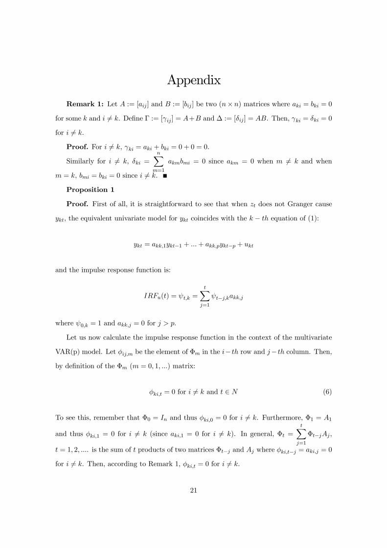
Proposition 1

Proof. First of all, it is straightforward to see that when zt does not Granger cause

ykt, the equivalent univariate model for ykt coincides with the k − th equation of (1):

ykt = akk,1ykt−1 + ...+ akk,pykt−p + ukt

and the impulse response function is:

IRFu(t) = ψt,k =tX

j=1

ψt−j,kakk,j

where ψ0,k = 1 and akk,j = 0 for j > p.

Let us now calculate the impulse response function in the context of the multivariate

VAR(p) model. Let φij,m be the element of Φm in the i− th row and j− th column. Then,by definition of the Φm (m = 0, 1, ...) matrix:

φki,t = 0 for i 6= k and t ∈ N (6)

To see this, remember that Φ0 = In and thus φki,0 = 0 for i 6= k. Furthermore, Φ1 = A1

and thus φki,1 = 0 for i 6= k (since aki,1 = 0 for i 6= k). In general, Φt =tX

j=1

Φt−jAj ,

t = 1, 2, .... is the sum of t products of two matrices Φt−j and Aj where φki,t−j = aki,j = 0

for i 6= k. Then, according to Remark 1, φki,t = 0 for i 6= k.

21

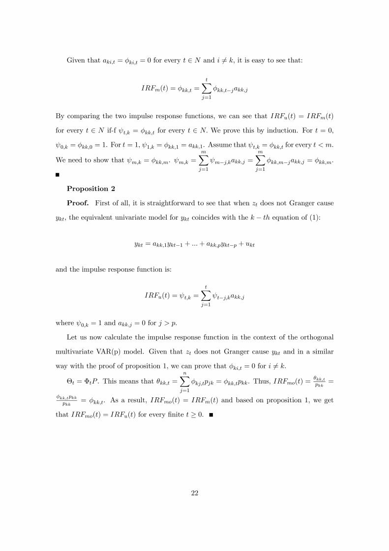
Given that aki,t = φki,t = 0 for every t ∈ N and i 6= k, it is easy to see that:

IRFm(t) = φkk,t =tX

j=1

φkk,t−jakk,j

By comparing the two impulse response functions, we can see that IRFu(t) = IRFm(t)

for every t ∈ N if-f ψt,k = φkk,t for every t ∈ N. We prove this by induction. For t = 0,

ψ0,k = φkk,0 = 1. For t = 1, ψ1,k = φkk,1 = akk,1. Assume that ψt,k = φkk,t for every t < m.

We need to show that ψm,k = φkk,m. ψm,k =mXj=1

ψm−j,kakk,j =mXj=1

φkk,m−jakk,j = φkk,m.

Proposition 2

Proof. First of all, it is straightforward to see that when zt does not Granger cause

ykt, the equivalent univariate model for ykt coincides with the k − th equation of (1):

ykt = akk,1ykt−1 + ...+ akk,pykt−p + ukt

and the impulse response function is:

IRFu(t) = ψt,k =tX

j=1

ψt−j,kakk,j

where ψ0,k = 1 and akk,j = 0 for j > p.

Let us now calculate the impulse response function in the context of the orthogonal

multivariate VAR(p) model. Given that zt does not Granger cause ykt and in a similar

way with the proof of proposition 1, we can prove that φki,t = 0 for i 6= k.

Θt = ΦtP . This means that θkk,t =nX

j=1

φkj,tpjk = φkk,tpkk. Thus, IRFmo(t) =θkk,tpkk

=

φkk,tpkkpkk

= φkk,t. As a result, IRFmo(t) = IRFm(t) and based on proposition 1, we get

that IRFmo(t) = IRFu(t) for every finite t ≥ 0.

22

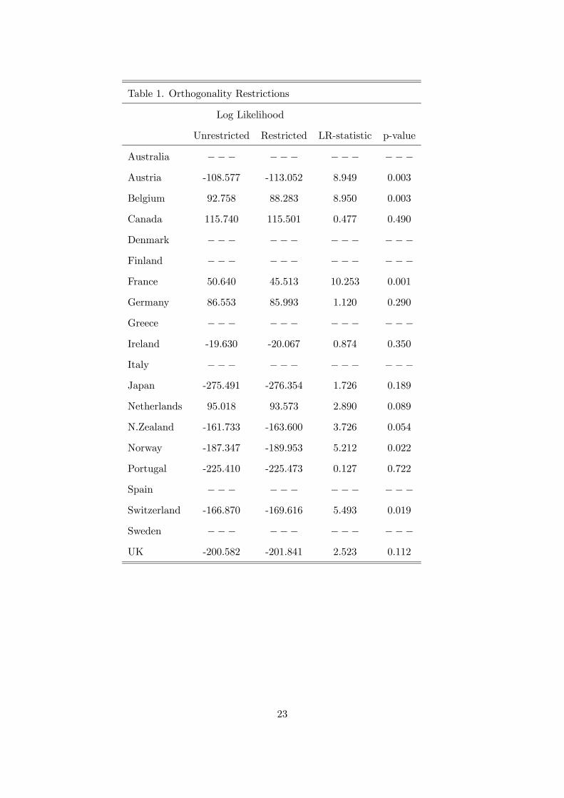
Table 1. Orthogonality Restrictions

Log Likelihood

Unrestricted Restricted LR-statistic p-value

Australia −−− −−− −−− −−−Austria -108.577 -113.052 8.949 0.003

Belgium 92.758 88.283 8.950 0.003

Canada 115.740 115.501 0.477 0.490

Denmark −−− −−− −−− −−−Finland −−− −−− −−− −−−France 50.640 45.513 10.253 0.001

Germany 86.553 85.993 1.120 0.290

Greece −−− −−− −−− −−−Ireland -19.630 -20.067 0.874 0.350

Italy −−− −−− −−− −−−Japan -275.491 -276.354 1.726 0.189

Netherlands 95.018 93.573 2.890 0.089

N.Zealand -161.733 -163.600 3.726 0.054

Norway -187.347 -189.953 5.212 0.022

Portugal -225.410 -225.473 0.127 0.722

Spain −−− −−− −−− −−−Switzerland -166.870 -169.616 5.493 0.019

Sweden −−− −−− −−− −−−UK -200.582 -201.841 2.523 0.112

23

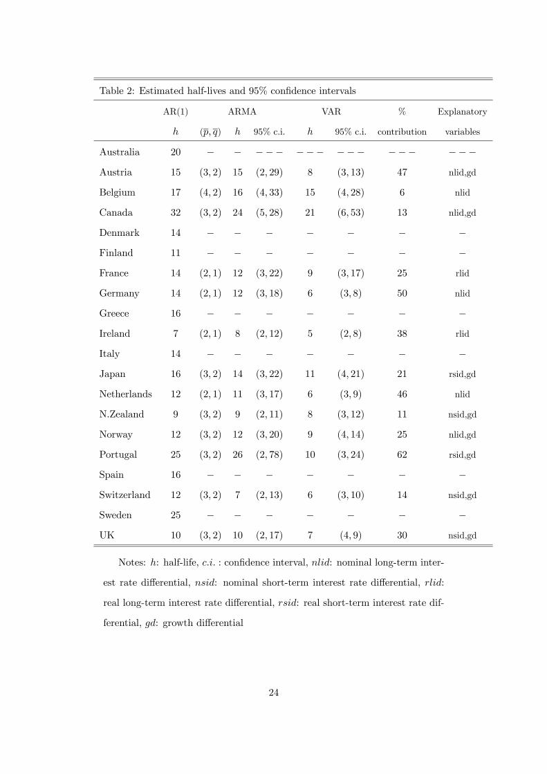
Table 2: Estimated half-lives and 95% confidence intervals

AR(1) ARMA VAR % Explanatory

h (p, q) h 95% c.i. h 95% c.i. contribution variables

Australia 20 − − −−− −−− −−− −−− −−−Austria 15 (3, 2) 15 (2, 29) 8 (3, 13) 47 nlid,gd

Belgium 17 (4, 2) 16 (4, 33) 15 (4, 28) 6 nlid

Canada 32 (3, 2) 24 (5, 28) 21 (6, 53) 13 nlid,gd

Denmark 14 − − − − − − −Finland 11 − − − − − − −France 14 (2, 1) 12 (3, 22) 9 (3, 17) 25 rlid

Germany 14 (2, 1) 12 (3, 18) 6 (3, 8) 50 nlid

Greece 16 − − − − − − −Ireland 7 (2, 1) 8 (2, 12) 5 (2, 8) 38 rlid

Italy 14 − − − − − − −Japan 16 (3, 2) 14 (3, 22) 11 (4, 21) 21 rsid,gd

Netherlands 12 (2, 1) 11 (3, 17) 6 (3, 9) 46 nlid

N.Zealand 9 (3, 2) 9 (2, 11) 8 (3, 12) 11 nsid,gd

Norway 12 (3, 2) 12 (3, 20) 9 (4, 14) 25 nlid,gd

Portugal 25 (3, 2) 26 (2, 78) 10 (3, 24) 62 rsid,gd

Spain 16 − − − − − − −Switzerland 12 (3, 2) 7 (2, 13) 6 (3, 10) 14 nsid,gd

Sweden 25 − − − − − − −UK 10 (3, 2) 10 (2, 17) 7 (4, 9) 30 nsid,gd

Notes: h: half-life, c.i. : confidence interval, nlid: nominal long-term inter-

est rate differential, nsid: nominal short-term interest rate differential, rlid:

real long-term interest rate differential, rsid: real short-term interest rate dif-

ferential, gd: growth differential

24