deckling formulating two-stage, two- machine … · tappsa journal | volume 1 2012 31 deckling...

TAPPSA JOURNAL | VOLUME 1 2012 31

DECKLING

Formulating two-stage, two-machine deckling with compact LP

Adolf Diegel, Cutline Research, 66 Edmonds Road, Durban 4001Corresponding author, [email protected], www.cutworks7.com

Olaf Diegel, Massey University, Auckland, [email protected], www.massey.ac.nz

Abstract

Deckling or cutting stock problems involve large units to be split into small ones. We aim to reduce stock usage and setups, favour long runs, surplus over waste, low pattern loss, few order splits as well as prompt delivery. We may also have to respect trade tolerance or keep pattern loss within the width of a disposal chute. Finally, when sheets are to be made or reels too narrow for a winder’s knife settings, we generate parent reels (cutreels) for the winder, to be deckled again on a second cutter or re-reeler,

“two-stage”, involving two machines.

Beyond its running cost, a cutter wastes trim at each edge, so cutreels should be as wide as possible. But wide units may fit the winder poorly: one machine’s settings may impair the other’s efficiency. So we include winder broke, second-stage trim and reels-in-cutreels in a compact LP-routine to quantify conflicting objectives. A companion paper does this for compulsory or optional cutreels and portrait or landscape sheets.

Keywords: Deckling, Cutting stock, Two-stage, two-machine optimisation.

Introduction: Deckling in a paper mill

We study paper cutting because orders come by the tonne, so any savings matter. Paper also leads to other materials (Diegel 2011a), each with its own constraints, some going beyond the classic Trim Loss Problem (Paul 1956). Paper cutting is also the topic analyzed by Zak (2002).

To appreciate the reasons for successive machines in cutting paper, one should observe a paper machine. Wet pulp enters, dry paper exits so fast that it can be wound, but not slit. The output is a machine roll, pope-reel or jumbo, a unit so large in width and diameter and so heavy that it cannot be shipped. The first task is to rewind a jumbo into smaller sets: “stock units” or “rolls”, to become narrow “reels”.

This is done on a winder, in first-stage deckling. It is often called “cutting”, yet it involves several steps. Cores are supplied and blades set by a winder crew or by automated devices. The winder unwinds a jumbo and, while slitting the paper, rewinds it. Rewinding runs so fast that the winder can only deckle (unwind, slit and rewind). It cannot chop sheets, nor can it slit very narrow reels, below its knife settings.

Some reels may be shipped as they come off the winder, wide as they are, “saleable reels”. Others go to a second machine. They are “re-reelers”, to be deckled again into narrow reels, or “cutreels” to be unwound, slit lengthwise and chopped crosswise into sheets. (Cutreel reels cease to be reels upon chopping, but they are counted as reels when converting tonnes by diameter and GSM, “grammes per square metre”.) Finally, “coated papers” and “laminates” are re-reelers rewound in fixed multiples.

A second-stage machine works like the first one: it unwinds and slits wide rolls, to rewind narrow reels or to chop sheets. Yet, to simplify terms, we use “winder”, then “cutter” for both re-reeler and chopper.

Winder and cutter efficiency reflect distinct cost factors. On both, a poor fit wastes energy. On a winder, it leaves unused material, “broke”, to be pulped. On a cutter, material is wasted, too, “trim”, taken off each side to make smooth edges. Trim is fixed, so, for the same output, narrow units entail more waste and longer runs.

Thus deckling was initially called “The Trim Problem” (Paul 1956, Cheng 1994): it concerned a winder and “trim” was used for waste. We separate cutter trim from winder

32 TAPPSA JOURNAL | VOLUME 1 2012

DECKLING

broke. Except perhaps for single reels, trim is inevitable. At best we can reduce its total by forcing cutreels to their greatest width. Yet good deckling may minimise winder broke.

In short, we must account separately and explicitly for broke and trim, to balance the efficiency of both stages. Narrow units tend to fill the winder, but leave the cutter at a fraction of its capacity and with much trim. Yet wide cutreels may not fit the winder: as one machine’s cost goes up, the other’s goes down and a graph would show this in curves. Combining them yields the classic U-shaped total cost curve.

Computational aspects

A stock roll being in a horizontal position, we show a cutting plan in the same way, its reels side by side as they come off a winder. Figure 1 presents such a plan for the data quantified in Table 1.

This plan lists the reel widths at hand, nett usable stock width, then demand. Patterns come with their label and frequency or run length. The first has 13 runs of 600*5 + 400*2 = 3800 mm with 80 mm loss. Then the other pattern obtains the reels not provided by Pattern 1.

A plan’s bottom line summarises all runs. First come the rolls used. Then follow the reels obtained for each width. Totals may differ from demand, with surplus (or deficit, once it is allowed): 80 400s are on order, 13*2 + 7*8 or 82 are output, with 2 extra reels. Finally, the bottom line ends with total loss (broke, pulp or scrap).

The quantitative plan uses n-up, reel frequency. Here it is (5 2), then (1 8), eventually covering all possible patterns.

Figure 1. Simple picture-type cutting plan

Table 1. Quantitative plan: orders, pattern and

reel frequency, output

Generally,ai, a pattern with each reel’s number up, possibly zero and (i = 1 to m), the number of sizes on order;

xj, the run length or frequency of cutting pattern j, (j = 1 to n), any one pattern among n generated. Then

∑(aij * xj) ≥ di, total stock usage, to be minimised while filling demand for all orders.

If such a formulation applied to EOQ, the Economic Order Quantity, its derivative would yield one deterministic solution.

Not so here: we deal with Finite Mathematics (Kemeny 1962) and Linear Programming. It uses a flow diagram as in Kemeny’s second edition (1972, p. 283) for Compact LP (without explicit identity matrix) to invert an initial to a final table and to guarantee minimal stock usage.

Yet unlike a derivative with one result, LP may yield many, depending on how one starts. In our context, optimal plans minimise stock, but they may differ in setups, run length, pattern loss, order spread and splits (Diegel 2011b), even total loss: minimal stock may yet allow much loss, to be traded for surplus and other criteria, as will be seen shortly.

But before we turn to solutions, we present our LP-table (“tableau” in most textbooks). Its data are those from Table 1 for a winder, one-stage to begin with. As in a quantitative plan, patterns appear row by row (Diegel 1987, 1988, 1996). Also, Table 2 lists all possible patterns as each will appear in at least one of the plans in Table 3 (see following page).

In the initial tableau, heading rows list the widths of reels


DECKLING

and stock, then demand, negative, “unfilled”, to be filled by patterns. Wanted are 72 reels of 600 mm and 80 400s. Then -20 in the 3880-column is the lowest possible stock usage: total demand is 600*72 + 400*80 or 75200 mm; dividing by 3880 rounds up to 20 rolls. These enter as -20, a “demand” to use so much stock. (20 rolls make 77600, so 2400 mm remain as “slack”, to cover broke or possibly surplus.)

Reels and demand are followed by patterns, row by row. Their labels are negative to distinguish patterns from reel widths. A label starts with the pattern’s consecutive number, then includes its number of reels, here 06 to 09. Column 2 at left has pattern loss: 600*6 reels in 3880 stock leave an offcut of 280 mm. Pattern -106 supplies 6 reels of 600 mm, no 400s, then 1 to the “demand” to use 20 rolls. And so on.

Selectively inverting the initial tableau exchanges demand

for patterns, at right in Table 2: -207 & -609 run 13 and 7 times to yield 72 600s and 82 400s, with 2 surplus reels of 400 mm and 1600 mm total loss. Thus the initial “slack” of 2400 mm covered this loss plus 800 mm surplus.

Space prevents us from exploring LP, but its results are clear: orders were replaced by patterns, demand by run lengths or surplus. This was done selectively, to favour long runs and little waste.

Opportunity costs, alternative solutions

Initial choices determine a final plan. Yet once it was found, others may emerge from exploring opportunity costs (shadow prices) and exchange coefficients. To study these, we kept all feasible patterns in Table 2. (In fact, only a few “good” patterns were generated dynamically, “column generation” when patterns were in columns, Gilmore 1961).

Table 3. 10 alternative cutting plans for 2 orders

Table 2. First and last LP-tableau for simple data


DECKLING

Thus we note that pattern -408 at right in Table 2 has 0 loss: it will not change total loss, but other aspects of the solution. To enter this pattern, we pivot on row -408 and column -609, replacing 7 runs of one by 7/.50 or 14 runs of the other. This simultaneously reduces -207 from 13 runs to 6. We show the original plan and 9 alternatives in Table 3.

Patterns have their labels from Table 2, including n-across: three plans need as many as 9 and the others 8 reels in at least one pattern. This becomes critical below (when we do not have so many knives).

Here we note that each plan is unique in at least one aspect: surplus, pattern loss and total loss, setups, run length, order splits (Diegel 2005, 2006a, 2009, 2011c, 2011d, Goulimis 1990). Yet we do not now choose a “best” plan, nor do we initially know how to find it. We do show that 2 orders may yield at least 10 plans.

Thus LP differs from formal methods with a deterministic outcome. LP depends not on derivative and integral, but on informed programming.

Compulsory and optional re-reeling

There are two reasons for machines to run in tandem. One is technical, to make re-reeling compulsory; the other reflects cost, the optional case. We should understand the difference to relate to previous work.

Re-reeling is inevitable for very narrow reels, those below a winder’s knife settings: they are unwound, slit

and rewound on a second cutter. Similarly for sheets: the winder runs so fast that it can slit only, so sheets must be chopped crosswise on a chopper. Finally, some materials come too fast off a primary machine to be made to their final size: steel (Ferreira 1990) or foil, film or wrap (Diegel 2009, 2011a).

The optional case occurs when winder knives are “too few” rather than “too wide” for the orders on hand: “The need for two stages is due to a limited number of slitters on the winder” (Zak 2002, p. 1144).

To illustrate, consider reels of 300 mm. They cannot come off a winder with wide knife settings, but are combined as cutreels for the winder, to be slit on a second cutter. One of 2080 mm with 20 mm trim can run up to 6 reels: 300*6 plus trim makes 1820, then 1520, 1220, 920 or 620 mm cutreels. A 4400 mm winder fills an order for 560 reels with 3 cutreels on the winder, 1820*2 + 620, and 40 stock rolls, Plan A in Figure 2.

For the optional case, we take a winder which can slit 300s, but note that 4400/300 is 14: even a modern winder may not have enough knives. If it can do at most 8 reels at once, 8*300 is 2400 and 4400 - 2400 leaves 2000 mm unused. We rather use this offcut for a 1820 mm cutreel. Can we do with this one optional cutreel? See Plans B and C.

All plans yield 14 final reels from each pattern, to use 40 stock rolls for 560 reels. Plan A has only cutreels because its winder cannot slit any 300s, compulsory re-reeling. For the optional case, we start with Plan B. It repeats A except for a 620-cutreel: this winder can do 300s, so why

Figure 2. Winder plans for compulsory and optional re-reelers


DECKLING

waste time, energy and trim in sending them to a cutter? B has two 1820s because we know from A that they fit well and use the cutter fully; also, with 2 cutreels and 2 simple reels we run only 4 across.

Should the extra cutreel be 1820 or 620, as in Plan C? It would be 1820 if reels must be shipped in 6-packs. Otherwise a 620-cutreel for 2 300s reduces re-reeling from 6 + 6 to 6 + 2. 6 300s can come off the winder at no cost. More critically, it is a total of 40*6 or 240 reels.

Cutter runs may not be as expensive as a winder’s, but, beyond energy and trim, they entail storage, extra handling and work in process. So, to minimise total cost, compulsory cutreels should be wide, to fill demand with minimal trim and few cutreel runs.

In the optional case, few winder knives may impose cutreels, yet we aim to reduce their output, ideally to zero. This means distinct objectives: minimise any cutreels as against narrow cutreels.

To implement either objective, it is not enough to minimise trim. As in Plans B and C, it is the same for the same number of cutreels. Rather, to minimise reels-in-a-cutreel, we must count them explicitly.

Previous work

The papers mentioned below cover one objective or the other. Zak defines optional re-reeling, others consider a compulsory second stage. This may reflect the facts of making steel, for example; but slitting it admits cutreels as well as paper does. Also, all papers start with LP, but add other methods for stage 2, as quoted in chronological order.

The earliest reference we found is Haessler (1971, submitted 1969). Yet in (1979, p. 145) he states: “This problem has not been discussed in the literature even though it occurs in a number of industries.” Then, “A computer programme that employs a number of heuristics in conjunction with a linear programming algorithm was developed...” (1979, p. 148).

Ferreira et al. (1990) call “two-phase” a case in the iron and steel industry. For stage 2 they propose a heuristic “based on an automatic sequential search” and claim that the inclusion of second-stage costs makes “a nonlinear cutting stock problem” (p. 185).

de Carvalho and Rodrigues (1995) deal with a compulsory second phase in steel making, separate “first phase” broke from “second phase” trim and propose an LP-model combined with knapsack subproblem simulation.

Zak (2002, submitted March 2000) was quoted above for the optional case. For stage 2 he adds rows for “intermediate rolls” to his stage 1 table. Extra columns cover “a non-linear knapsack problem” (p. 1143).

Correia et al. (2004), who co-authored with Ferreira (1990), similarly approach “Reel and sheet cutting at a paper mill”.

“An effective solution for a real cutting stock problem in manufacturing plastic rolls” (Varela et al., 2009) covers compulsory re-reeling to “propose a heuristic solution based on a GRASP algorithm ... and a Sequential Heuristic Randomized Procedure (SHRP)” (p. 125). “Neither underproduction nor overproduction is allowed for any of the orders”, but “a number of additional rolls ... should be explicitly permitted by the expert, to be stored in the shop stock” (p. 127).

We do not use any of the auxiliary methods listed above, but optimise re-reeling with the LP-routine for one-stage problems. We merely add 2 columns for reels-in-cutreels, then count all of them for the optional case, narrow ones otherwise, as explained below.

Introducing our approach: cutreels from reels

Our example’s orders and winder data are from Zak (2002, p. 1152), but in mm. They appear at the top of a cutting plan, notably in Table 4. It repeats the first two plans from Table 3, those optimal if surplus is preferred to waste. The plans do differ: runs of 13 and 7 against 6 and 14, then “n-across”, maximal number of reels per pattern, 9 against 8.

Slightly different run lengths seem insignificant, but the winder crew does like long runs. Yet n-across is critical: here we prefer 9 across, but can safely do with 8 (even for 3 of the 5 exact plans at the bottom of Table 3). But what if we cannot run 8 reels across the winder?

We start with at most 7 reels: now knives are “too few” rather than “too wide”. Some 600s or 400s must be combined as cutreels on the winder, to be re-reeled. Which should it be? How many? To find an answer, we

Table 4. Two good winder plans if surplus is preferred to waste


DECKLING

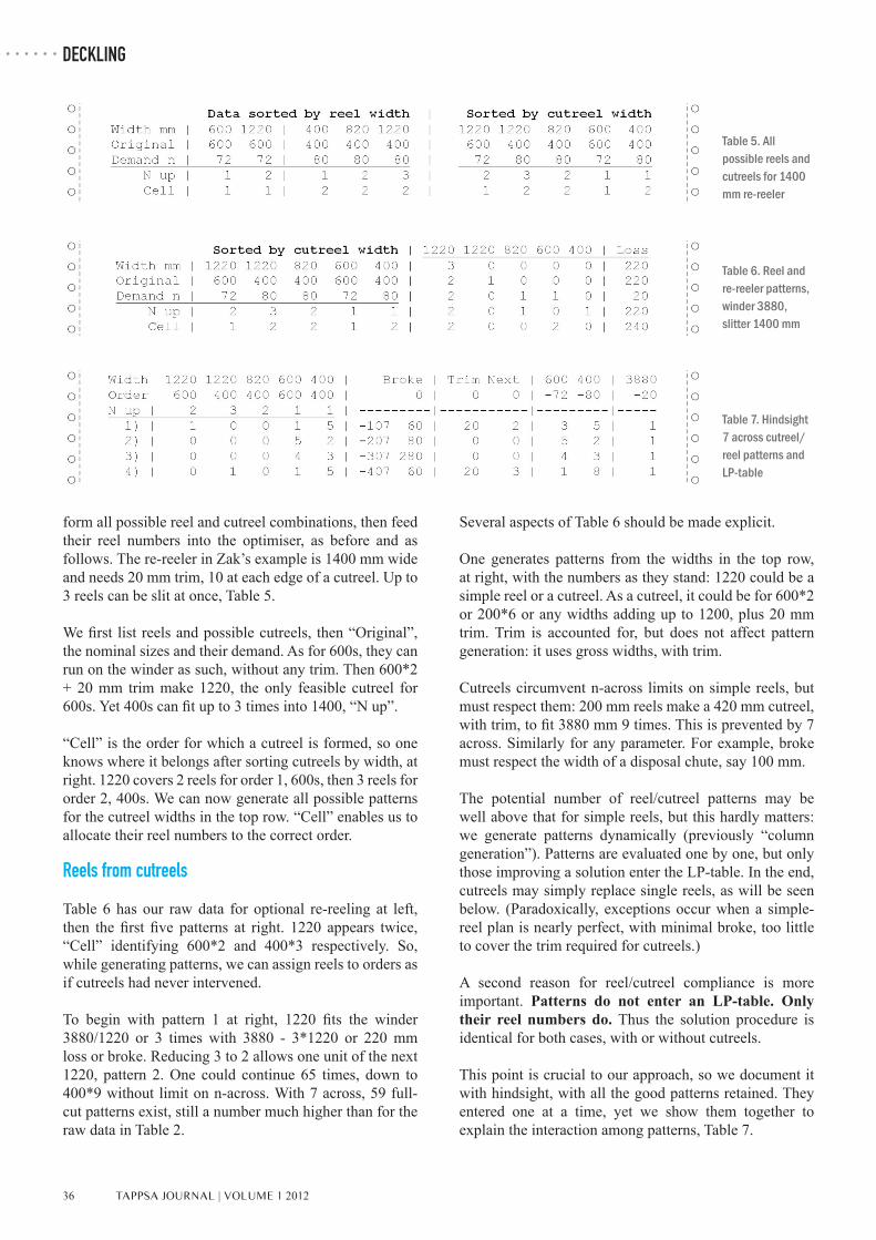
form all possible reel and cutreel combinations, then feed their reel numbers into the optimiser, as before and as follows. The re-reeler in Zak’s example is 1400 mm wide and needs 20 mm trim, 10 at each edge of a cutreel. Up to 3 reels can be slit at once, Table 5.

We first list reels and possible cutreels, then “Original”, the nominal sizes and their demand. As for 600s, they can run on the winder as such, without any trim. Then 600*2 + 20 mm trim make 1220, the only feasible cutreel for 600s. Yet 400s can fit up to 3 times into 1400, “N up”.

“Cell” is the order for which a cutreel is formed, so one knows where it belongs after sorting cutreels by width, at right. 1220 covers 2 reels for order 1, 600s, then 3 reels for order 2, 400s. We can now generate all possible patterns for the cutreel widths in the top row. “Cell” enables us to allocate their reel numbers to the correct order.

Reels from cutreels

Table 6 has our raw data for optional re-reeling at left, then the first five patterns at right. 1220 appears twice, “Cell” identifying 600*2 and 400*3 respectively. So, while generating patterns, we can assign reels to orders as if cutreels had never intervened.

To begin with pattern 1 at right, 1220 fits the winder 3880/1220 or 3 times with 3880 - 3*1220 or 220 mm loss or broke. Reducing 3 to 2 allows one unit of the next 1220, pattern 2. One could continue 65 times, down to 400*9 without limit on n-across. With 7 across, 59 full-cut patterns exist, still a number much higher than for the raw data in Table 2.

Table 5. All possible reels and cutreels for 1400 mm re-reeler

Table 6. Reel and re-reeler patterns, winder 3880, slitter 1400 mm

Several aspects of Table 6 should be made explicit.

One generates patterns from the widths in the top row, at right, with the numbers as they stand: 1220 could be a simple reel or a cutreel. As a cutreel, it could be for 600*2 or 200*6 or any widths adding up to 1200, plus 20 mm trim. Trim is accounted for, but does not affect pattern generation: it uses gross widths, with trim.

Cutreels circumvent n-across limits on simple reels, but must respect them: 200 mm reels make a 420 mm cutreel, with trim, to fit 3880 mm 9 times. This is prevented by 7 across. Similarly for any parameter. For example, broke must respect the width of a disposal chute, say 100 mm.

The potential number of reel/cutreel patterns may be well above that for simple reels, but this hardly matters: we generate patterns dynamically (previously “column generation”). Patterns are evaluated one by one, but only those improving a solution enter the LP-table. In the end, cutreels may simply replace single reels, as will be seen below. (Paradoxically, exceptions occur when a simple-reel plan is nearly perfect, with minimal broke, too little to cover the trim required for cutreels.)

A second reason for reel/cutreel compliance is more important. Patterns do not enter an LP-table. Only their reel numbers do. Thus the solution procedure is identical for both cases, with or without cutreels.

This point is crucial to our approach, so we document it with hindsight, with all the good patterns retained. They entered one at a time, yet we show them together to explain the interaction among patterns, Table 7.

Table 7. Hindsight 7 across cutreel/reel patterns and LP-table


DECKLING

At left are 7 across patterns, 1 + 1 + 5, 5 + 2 or 4 + 3, so all labels end on “07”. Yet at right we have up to 9 reels. Is this correct? It is because a cutreel contains several simple reels, 600*2 or 400*3 in 1220, at the cost of trim and a second run. Yet the cost has a benefit: few cutreels yield many reels, hence our heading, “reels from cutreels”. Only reels enter the LP-table, to fill demand. The optimiser does not care about a reel’s origin. We do: the care is reflected in the new columns, “Trim” and “Next”.

“Trim” records what is due to cutreels, “Next” the reels for stage two. Patterns 2 and 3 have simple reels, with 0 for Trim and Next. Patterns 1 and 4 need the same 20 mm trim for one cutreel, yet it yields 2 reels in pattern 1, then 3 in pattern 4, Next. So minimising trim favours few and wide cutreels, hence many reels for stage 2. Few are wanted for optional re-reeling, so Next is the dominant objective, with priority over Trim. Trim and Next are the only stage 2 columns added to our table (we do not add Zak’s indefinite number of rows for “intermediate rolls”). In turn, the new columns are updated just like any others in an LP-table.

Two-stage interaction

The interaction between two stages is quantified by opportunity costs. Table 8 clarifies these by keeping patterns next to the initial tableau. We used patterns 1 and 2 to fill demand and, in step 3, exchanged unused stock for surplus, 400*2. The dynamic table would hold only patterns 1 and 2, but we included 3 and 4 to study their potential.

The initial solution runs patterns -107 and –207, 14 & 6 times, to fill demand and yield 2 surplus 400s. 14*60 +

6*80 makes 840 + 480 or 1320 mm broke, then 14*20 or 280 mm trim for pattern 1. 14 runs of that pattern include a 1220 mm cutreel for 600*2: 14*2 or 28 reels will come off a re-reeler, “Next”, reels which need a next or second stage.

Can we reduce re-reeling? The “Next”-column has -1 for patterns 3 and 4: each run saves 1 reel. How often can they run? We check their critical ratio: we could exchange -307 for surplus 400s 2/-.50 or -4 times, or else -407 for -107, 14/-2 or -7 times. Either number is multiplied by the Next-coefficient to yield the “Nett effect of pattern on Next”:

Next-coefficient * Critical Ratio, -1 * 2/-.5 = -1*-4 = 4, pattern 3.

We double-check this by placing the original simple-reel plan from Table 3 next to the initial cutreel plan, Table 9.

The main conclusion is this: simple and cutreel plans are functionally identical. The 3-up 600s at left became a 600*2 cutreel and 1 simple reel. Thus the cutreel plan at right has less broke than the original, but it needs 280 mm trim and 1320 + 280 = 1600 mm total loss. Trim is for 14 cutreels in Pattern 1 and 14*20 = 280, the total from Table 8.

As for final output, consider 400s: all are simple reels and 14*5 + 6*2 makes 82, 2 surplus reels beyond 80. Yet 600s come in 2 lots: 14 runs of a 1220-cutreel with 2 reels, so 14*2 = 28, then 14*1 + 6*5 or 44 from the winder, and 28 + 44 = 72. Demand is filled, but 14 cutreels go to a second stage. They cost energy and time, plus the handling of 28 reels which could have been shipped as they came off the winder.

Table 9. First good 8 across winder

plan and its 7 across version

Table 8. 7 across patterns, initial

tableau and first solution

38 TAPPSA JOURNAL | VOLUME1 2012

DECKLING

Can we reduce the number of reels requiring extra handling? “Nett effect” in Table 8 suggests that patterns 3 and 4, each on its own, can save 4 and 7 reels. We check the larger effect from pattern 4 in Table 10: the very best winder plan (with more equal runs, Table 3) corresponds to a good cutreel plan: instead of 14*2 or 28 reels for stage 2, there are only 21, confirming 7 reels “nett effect” computed in Table 8.

Similarly, enforcing pattern 3 would make a cutreel plan with 28 - 4 or 24 next runs, with 4 as “nett effect”. It is less obvious that patterns 2, 3 and 4 together yield the plan in Table 11.

Cutter performance is optimal, with only 18 optional re-reelers instead of 28 in the initial solution, a nett saving of 10. (10 is not 4 + 7, the cumulative “nett effect” of patterns 3 and 4. When two patterns are added at once, the LP-table is revised, simultaneously.) Yet to reduce 21 to 18 cutter runs we need an extra setup and lose two surplus 400s.

Comparing results: Technical or cost-related performance?

We have seen that second stage cutting can be minimised, absolutely. Yet does it dominate efficiency? What about stock usage, setups, run length and surplus? These are to be accounted for, by assessing their cost, but space obliges us to cover this topic elsewhere (Diegel 2006b, 2011e).

What we can do here is reduce n-across until it becomes tight enough to increase stock usage. Our best plans began

Table 10. Best 9 across winder plan and its 7 across version

Table 11. Poor no-limit winder plan and best 7 across version

Table 12. N-across and winder vs cutter results for 20, then 21 rolls

with 9 across and good runs, 13 and 7. These change to 14 and 6 with 8 across, but stock usage, broke and surplus are the same. 7 across affects setups, but maintains stock usage even though cutreels require trim. This is so because of initial “slack”, a gap between demand and minimal stock usage, 2400 mm. Slack covers broke plus trim down to 4 across, as shown in Table 12 for fewer and fewer knives. At 3 across, 4620 mm broke require 21 stock rolls.

Critical are the columns at right: “Simple” and “Cutreel” are winder reels, then “Re-reel” the 600 or 400 mm reels slit on the cutter. Simple reels decline from 154 to 24 and 0, the rest to be re-reeled. 3 across and 21 rolls yield 72 600s and 81 400s or 153 reels to be re-reeled. So winder results are steady from 9 to 4 across, but stage 2 costs increase in cutreels (hours) and the handling of so many more re-reelers.

It is also critical that we keep 24 simple reels at 4, the lowest feasible n-across for 20 rolls. Zak has all reels re-reeled (2002, p. 1154). To document this, Table 13 has the 4 across plans for both procedures.

Zak’s plan has less winder broke, 880 against 1280 mm, yet so much cutter trim that total loss is the same: 880 + 1520 and 1280 + 1120 add up to 2400 mm. More trim means more cutter runs, 1520/20 against 1120/20 mm or 76 against 56, 20 extra second-stage cutter runs.

In our plan, some 600 mm reels do come from 1220-cutreels, 48 of them, 16*1*2 + 4*2*2 from both patterns. 24 come off the winder, 16*1 + 4*2. Output equals demand, 48 + 24 or 72 for 600s and 48 + 32 or 80


DECKLING

for 400s. The same applies to Zak’s totals, but all reels are re-reeled, at the extra cost of slitting 600 + 400 in a 1020-cutreel.

In short, winder broke is not the main objective in two-stage problems. One must also count cutreels, narrow ones in the compulsory case, all reels-in-cutreels for optional re-reeling. As for an absolute minimum, on the one hand, we have shown that we can find it; on the other hand, how far to go is a matter of balancing cutter against winder efficiency.

We would test our programme against others, but none are available. As a colleague wrote, “Concerning your surprise that so little seems to have been published in this area, I think it’s because practitioners have had to tackle this issue in practice, but have been loath to publish”. Our optimiser can be downloaded from www.cutworks7.com.

Summary

We have integrated two-stage, two-machine deckling in one optimiser. Our approach is based on “reels being reels”, whether they are slit on a first-stage winder or a second-stage cutter. After generating a cutreel pattern, for each cutreel we count how many reels it contains, then add these to simple reels in the same pattern: the sum enters an LP-table by pattern and order number. The table holds reels only, whether they come simply or from cutreels. It is the same as in one-stage winder deckling, but has two new columns for second-stage objectives.

We used data primarily for optional re-reeling (with few winder knives). Other examples of the interaction between the efficiency of two stages are found in “Two-stage optimisation” (Diegel 2006b, 2011e).

References

A search for our topic is complicated by “stage” covering “multistage” and “two or more dimensions” (Gilmore 1965, Below 2003), but neither means two dimensions (Diegel 1984) nor two machines. “Second phase” also covers “uncertain demand” (Demirci 2006). Among those with two machines, we find “nonlinear” (Haessler 1971), “multistage” (Zak 2002) or “two-phase” without “two” in the paper’s title (Correia 2004). Wäscher’s “improved typology” includes “Second-Level Standard Problems” (2007, pp. 1112-1113), but these cover stock of “different

sizes”, not a second machine. The two-machine case is not mentioned, while two or more stock sizes can be part of a one-stage formulation (Diegel 1984, 2007). Below, G. and G. Scheithauer (2003). Models with variable strip widths for two-dimensional two-stage cutting. www.math.tu-dresden.de/~capad/PAPERS/03-varwidth.pdf, 25 September 2003. Cheng, C. H., B. R. Feiring and T. C. E. Cheng (1994). The cutting stock problem - a survey. Int. Journal of Production Economics 36:291-305. Correia, M. Helena, Jose F. Oliveira and J. Soeiro Ferreira (2004). Reel and sheet cutting at a paper mill. Computers and Operations Research 31 8:1223-1243. Demirci, Mehmet C., Brady Hunsaker, Andrew J. Schaefer and Jay M. Rosenberger (2006). Column Generation within the L-shaped Method for Stochastic Linear Programmes. Under review, p. 14. Diegel, Adolf (1984). Optimal dimensions of virgin stock in cutting glass to order. Decision Sciences, The Journal for the American Institute of Decision Sciences 15 2:260-274. Diegel, Adolf (1987). Cutting paper in Richards Bay: Dynamic local or global optimization in the trim problem. ORiON Journal of the Operations Research Society of South Africa 3 1:42-55. First presented at Annual Meeting, ORSA, University of Cape Town, 1986. Diegel, Adolf (1988). Integer LP solution for large trim problems. Paper presented at EURO/TIMS, Paris, 6-8 July 1988. Diegel, Adolf, Edouard Montocchio, Edward Walters, Sias van Schalkwyk and Spurs Naidoo (1996). Setup minimising conditions in the trim loss problem. European Journal of Operational Research 95:631-640. Diegel, Adolf, Garth Miller, Edouard Montocchio, Sias van Schalkwyk and Olaf Diegel (2006a). Enforcing minimum run length in the cutting stock problem. European Journal of Operational Research 171:708-721. Presented at EURO/INFORMS, Istanbul 6 July 2003. Diegel, Adolf, Garth Miller, Edouard Montocchio, Sias van Schalkwyk, George Pritchard and Olaf Diegel (2006b). Two-stage optimization of the cutting stock problem. 3rd ESICUP meeting, Porto 16-18 March 2006.

NOTE: Due to space constrictions, the full list of references for this paper has not been published. To receive the complete list of references, please email the Editor at [email protected]

Table 13. Winder plans for our’s and Zak’s approach, 4 across

deckling formulating two-stage, two- machine … · tappsa journal | volume 1 2012 31 deckling...

Documents