decision-theory for crisis management - the air university
TRANSCRIPT

Decision-Theory for Crisis Management
| Final Report |
Mois�es Goldszmidt
(Principal Investigator and Program Manager)
Adnan Darwiche
(Principal Investigator)
Tom Ch�avez
David Smith
James White
Additional Participants:
John Breese, Denise Draper, Max Henrion, and Mark Peot
Rockwell Science Center
Palo Alto, CA 94301
(415) 325 7145
PIIN:
F30602-91-C-0031PR NO.
B-1-3356ARPA Order Number:
7741
E�ective Date of Contract:
February-01-1991
Contract Expiration Date:
September-30-1994
Amount of Contract:
$1,808,626.00
The views and conclusions contained in this document are those of the
authors and should not be interpreted as representing the official poli-
cies, either expressed or implied, of the Advanced Research Projects
Agency or the U.S. Government.
i

Contents
1 Executive Summary 1
1.1 Plan Generation Results : : : : : : : : : : : : : : : : : : : : : : : : : : : 1
1.2 Plan Evaluation Results : : : : : : : : : : : : : : : : : : : : : : : : : : : 2
1.3 Plan Simulation Results : : : : : : : : : : : : : : : : : : : : : : : : : : : 3
2 Introduction: Decision-Theory for Crisis Management 4
3 Plan Generation 5
3.1 Conditional Planning : : : : : : : : : : : : : : : : : : : : : : : : : : : : : 6
3.2 Control of Planning Search : : : : : : : : : : : : : : : : : : : : : : : : : : 7
3.2.1 Operator graphs : : : : : : : : : : : : : : : : : : : : : : : : : : : 8
3.2.2 Operator relevance : : : : : : : : : : : : : : : : : : : : : : : : : : 10
3.2.3 Variable analysis : : : : : : : : : : : : : : : : : : : : : : : : : : : 10
3.2.4 Open condition ordering : : : : : : : : : : : : : : : : : : : : : : : 12
3.2.5 Recursion analysis : : : : : : : : : : : : : : : : : : : : : : : : : : 13
3.2.6 Postponing Con icts : : : : : : : : : : : : : : : : : : : : : : : : : 14
3.2.7 Con ict resolution strategies : : : : : : : : : : : : : : : : : : : : : 15
3.3 Partial Plan Evaluation : : : : : : : : : : : : : : : : : : : : : : : : : : : : 16
4 Plan Evaluation 18
4.1 Transportation Trade-o� Analyzer : : : : : : : : : : : : : : : : : : : : : : 20
4.2 Decision-Theoretic Modeling Tools in the CPE : : : : : : : : : : : : : : : 20
4.3 Course Of Action Trade-o� Analyzer : : : : : : : : : : : : : : : : : : : : 22
4.4 Sensitivity Analysis in Planning : : : : : : : : : : : : : : : : : : : : : : : 25
4.4.1 The Expected Value of Information : : : : : : : : : : : : : : : : : 26
4.4.2 Computing the Value of Information in Large Decision Models : : 26
5 Plan Simulation 29
5.1 Action Networks : : : : : : : : : : : : : : : : : : : : : : : : : : : : : : : 30
5.1.1 Introduction into action networks : : : : : : : : : : : : : : : : : : 31
5.1.2 Progress on Action Networks : : : : : : : : : : : : : : : : : : : : 31
5.2 Algorithms : : : : : : : : : : : : : : : : : : : : : : : : : : : : : : : : : : : 33
5.2.1 Introduction : : : : : : : : : : : : : : : : : : : : : : : : : : : : : : 33
5.2.2 Dynamic Conditioning : : : : : : : : : : : : : : : : : : : : : : : : 35
5.2.3 Prediction Algorithm: Speci�c to action networks : : : : : : : : : 36
5.2.4 Prediction Algorithm: Speci�c to order-of-magnitude networks : : 37
5.2.5 Bounded Conditioning : : : : : : : : : : : : : : : : : : : : : : : : 37
ii

6 Concluding Remarks 39
A Appendix: Relevant Papers 44
iii
List of Figures
1 A partial conditional plan. : : : : : : : : : : : : : : : : : : : : : : : : : 7
2 Operator graph for a simple propositional problem. : : : : : : : : : : : : 9
3 First-order Operator graph. : : : : : : : : : : : : : : : : : : : : : : : : : 11
4 Operator graph after variable analysis. : : : : : : : : : : : : : : : : : : : 12
5 Partial plans with recursion. : : : : : : : : : : : : : : : : : : : : : : : : 14
6 Search space relationships for �ve threat removal strategies. : : : : : : : 16
7 Propositional operator graph with operator costs. : : : : : : : : : : : : : 17
8 Partial plan with two open conditions. : : : : : : : : : : : : : : : : : : : 18
9 Model structure used in the Transportation Trade-O� Analyzer. : : : : : 19
10 An example of an in uence diagram in IDEAL-EDIT. : : : : : : : : : : 21
11 The graph describes the buildup of U.S. citizens at an assembly area. : : 22
12 Top level model for the NEO course of action analysis tool. The tool
generates graphs describing risks for U.S. citizens and estimates of trans-
portation times. : : : : : : : : : : : : : : : : : : : : : : : : : : : : : : : 23
13 Conceptual overview of the algorithm for estimating EVI. : : : : : : : : 27
14 Probability distribution on Z. : : : : : : : : : : : : : : : : : : : : : : : : 28
15 Schematic view of a plan simulation scenario. : : : : : : : : : : : : : : : 30
16 An example of an action network. : : : : : : : : : : : : : : : : : : : : : 32
17 Current realization of the Plan Simulator and Analyzer (PSA) tool. : : : 35
List of Tables
1 Summary of Rockwell's contributions to ARPI. : : : : : : : : : : : : : : : 1
2 Impact on scienti�c and applications communities and future plans. : : : 2
3 Operator de�nitions. : : : : : : : : : : : : : : : : : : : : : : : : : : : : : 8
iv

1 Executive Summary
The Rockwell Science Center's main contribution to the ARPA Planning Initiative
(ARPI) has been the development and application of decision theoretic concepts and
tools to the problem of military transportation and crisis planning. Real world planning,
like most complex problems, involves multiple competing objectives and uncertainty
about actual outcomes. Thus, e�ective operational tools for planning must be able to
e�ciently manage uncertainty and trade-o�s between competing objectives. Rockwell's
contributions span three main areas of the planning process: generation, evaluation,
and simulation. Contributions range from basic research results to application oriented
software tools for military transportation planning. These contributions are brie y enu-
merated in the sections below, and are summarized in Tables 1 and 2.
Planning Basic Advances Demonstrations & Deliverables
Subtask
Generation Conditional planning (First CNLP). Brie�ng atControl of planning search (Op. Graphs). Rome Labs 1993.
Evaluation of partial plans.
Evaluation Transportation Trade-o� IFD-3 Sept 1993.Analyzer Tool (TTA). ARPI Workshops
Course of Action Trade-o� 1992, 1993, and 1994.Analyzer Tool (COATA). Software training sessions
New Algorithms for for Rome Labs Manager,Sensitivity Analysis. Sept. 1993
TTA, IDEAL,IDEAL-DEMOS May 1992.
Simulation Uncertainty modeling over time. Site visit (Palo Alto) by
Suite of approximate and exact Rome Labs Manager,algorithms for inference. Sept 1994.
Table 1: Summary of Rockwell's contributions to ARPI.
1.1 Plan Generation Results
� Conditional planning. Developed and implemented the �rst algorithm for condi-tional partial order planning. The algorithm accepts a goal, initial conditions, and
Strips-like operators, extended to allow uncertain outcomes. It produces partially-ordered plans with conditional branches for observed uncertainties. Details of the
algorithm are in [37]. The ideas from this algorithm are now used in several other
planners and algorithms including [18, 20, 8]. See Section 3.1.
1

Planning Impact Future
Subtask Plans
Generation Techniques and methods in uenced Techniques being extended inother planners such as ARPA{MADE program.
[18, 20, 8, 27, 34, 29]. Part of Rockwell IR&D.
Evaluation Decision theoretical Graphical interfaces beingcomponent in TARGET. extended for in-house tools.
Simulation Uncertainty modeling techniques Extend simulation techniques to
being used by other generation.researchers [25, 1]. Applications to diagnosis
for Rockwell business divisions.
Table 2: Impact on scienti�c and applications communities and future plans.
� Control of planning search. Developed, implemented, and evaluated a numberof techniques to help control the combinatorial explosion that occurs in genera-
tive planning. The control techniques include smart ordering of open conditions,recognition and control of recursion, variable binding analysis, and smart resolu-tion of threats between operators. Descriptions of these techniques can be foundin [42, 44, 38, 41]. Several of these ideas are now being investigated in othergenerative planners [27, 34, 29]. See Section 3.2.
� Evaluation of partial plans. Developed a technique for estimating the value
of partially completed plans. This technique provides estimates of the cost andprobability of success of achieving di�erent possible subgoals that could occur fora problem. This information is then used to compute an estimate of the costand probability of success for a partial plan [41]. We are currently investigatingthis technique further for the generation of assembly plans in the ARPA MADE
project. See Section 3.3.
1.2 Plan Evaluation Results
� Software tools. During the course of the program Rockwell produced and made
available to the ARPI community a set of tools for utility modeling and decision
theoretic evaluation of plans. These include:
{ IDEAL, IDEAL-DEMOS. Domain independent decision theoretic soft-ware tools, which enable construction and evaluation of utility models (madeavailable to CPE in May 1992). Delivered to the Common Prototyping En-
vironment (CPE) (1992). See Section 4.2.
{ Transportation Trade-o� Analyzer (TTA). Utility models and inferencemachinery for computing trade-o�s between consumption of resources and
2
the expected time for the achievements of goals under uncertainty in the
transportation domain (delivered in May 1992). See Section 4.1.
{ Course Of Action Trade-o� Analyzer (COATA). Utility models and in-
ference machinery for the evaluation of courses of action in the noncombatant
evacuation domain. COATA constituted the decision theoretic component of
the \Theater-level Analysis, Replanning and Graphical Execution Toolbox"
(TARGET) for the third Integrated Feasibility Demonstration (IFD-3) (May
and September 1993). See Section 4.3.
� Sensitivity analysis. Developed a new approximation algorithm for uncovering
relevant data with respect to a given set of decisions and a course of actions. This
functionality has proven to be essential for building utility models in both COATA
and the TTA. See Section 4.4.
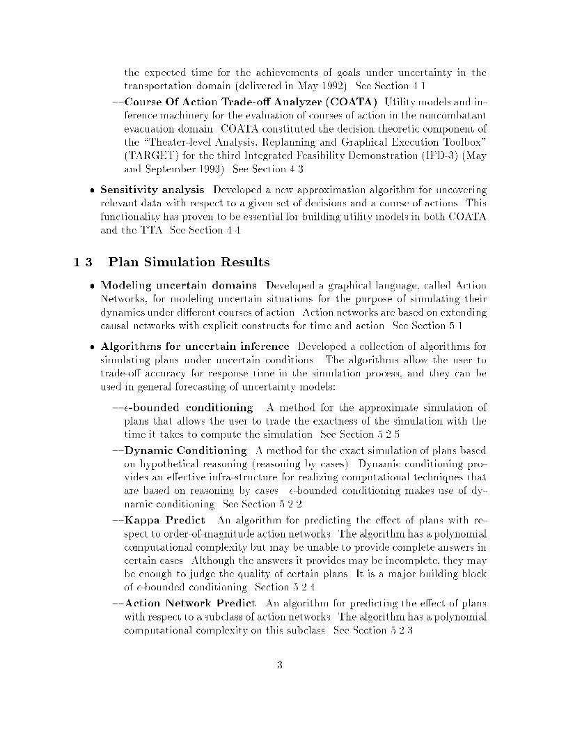
1.3 Plan Simulation Results
� Modeling uncertain domains. Developed a graphical language, called ActionNetworks, for modeling uncertain situations for the purpose of simulating their
dynamics under di�erent courses of action. Action networks are based on extendingcausal networks with explicit constructs for time and action. See Section 5.1.
� Algorithms for uncertain inference. Developed a collection of algorithms for
simulating plans under uncertain conditions. The algorithms allow the user totrade-o� accuracy for response time in the simulation process, and they can beused in general forecasting of uncertainty models:
{ �-bounded conditioning. A method for the approximate simulation ofplans that allows the user to trade the exactness of the simulation with thetime it takes to compute the simulation. See Section 5.2.5.
{ Dynamic Conditioning. A method for the exact simulation of plans basedon hypothetical reasoning (reasoning by cases). Dynamic conditioning pro-
vides an e�ective infra-structure for realizing computational techniques thatare based on reasoning by cases. �-bounded conditioning makes use of dy-
namic conditioning. See Section 5.2.2.
{ Kappa Predict. An algorithm for predicting the e�ect of plans with re-
spect to order-of-magnitude action networks. The algorithm has a polynomial
computational complexity but may be unable to provide complete answers incertain cases. Although the answers it provides may be incomplete, they maybe enough to judge the quality of certain plans. It is a major building block
of �-bounded conditioning. Section 5.2.4.
{ Action Network Predict. An algorithm for predicting the e�ect of planswith respect to a subclass of action networks. The algorithm has a polynomial
computational complexity on this subclass. See Section 5.2.3.
3
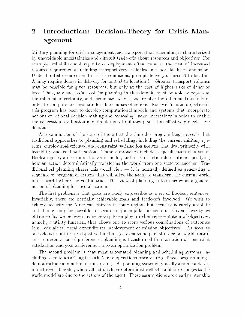
2 Introduction: Decision-Theory for Crisis Man-
agement
Military planning for crisis management and transportation scheduling is characterized
by unavoidable uncertainties and di�cult trade-o�s about resources and objectives. For
example, reliability and rapidity of deployment often come at the cost of increased
resource requirements, including transport crew, vehicles, fuel, port facilities, and so on.
Under limited resources and in crisis conditions, prompt delivery of force A to location
X may require delays in delivery for unit B to location Y . Greater transport volumes
may be possible for given resources, but only at the cost of higher risks of delay or
loss. Thus, any successful tool for planning in this domain must be able to represent
the inherent uncertainty, and formulate, weight and resolve the di�erent trade-o�s in
order to compute and evaluate feasible courses of actions. Rockwell's main objective in
this program has been to develop computational models and systems that incorporatenotions of rational decision making and reasoning under uncertainty in order to enablethe generation, evaluation and simulation of military plans that e�ectively meet these
demands.
An examination of the state of the art at the time this program began reveals that
traditional approaches to planning and scheduling, including the current military sys-tems, employ goal-oriented and constraint satisfaction notions that deal primarily withfeasibility and goal satisfaction. These approaches include a speci�cation of a set ofBoolean goals, a deterministic world model, and a set of action descriptions specifyinghow an action deterministically transforms the world from one state to another. Tra-
ditional AI planning shares this world view | it is normally de�ned as generating asequence or program of actions that will allow the agent to transform the current worldinto a world where the goal is true. This view of planning is too narrow as a generalnotion of planning for several reasons.
The �rst problem is that goals are rarely expressible as a set of Boolean sentences.Invariably, there are partially achievable goals and trade-o�s involved. We wish toachieve security for American citizens in some region, but security is rarely absolute
and it may only be possible to secure major population centers. Given these types
of trade-o�s, we believe it is necessary to employ a richer representation of objectives,
namely, a utility function, that allows one to score various combinations of outcomes(e.g., casualties, �scal expenditures, achievement of mission objectives). As soon as
one adopts a utility or objective function (or even some partial order on world states)as a representation of preferences, planning is transformed from a notion of constraint
satisfaction and goal achievement into an optimization problem.
The second problem is that most automated planning and scheduling systems, in-
cluding techniques arising in both AI and operations research (e.g. linear programming),
do not include any notion of uncertainty. AI planning systems typically assume a deter-ministic world model, where all actions have deterministic e�ects, and any changes to the
world model are due to the actions of the agent. These assumptions are clearly untenable
4

for military planning and scheduling. Action e�ects are not guaranteed because planes
can break down, ports can be bombed, and weather can be adverse, all in unpredictable
ways. Other agents, such as the enemy or some other threat, can interfere with ongoing
plans or actions in a non-deterministic manner. Therefore, mechanisms for addressing
uncertainty are necessary in a planning situation. To deal with this problem, existing
DOD planning exercises often assume a worst-case scenario in order to assess the impact
of an adverse outcome on the plan. Unfortunately, this strategy yields in exible plans
with sometimes unacceptable economical costs. In this project, we adopt probability as
a mechanism for modeling uncertainty. This provides a theoretically sound means for in-
corporating uncertainty, and allows us to utilize a number of well-established algorithms
for reasoning.
Rockwell activities in this program cover three main areas in planning technology:
1. Plan Generation. The objective behind this area of planning has been to re-search and develop general purpose planning systems suitable for military trans-portation planning and crisis management based on generalizing classical gener-
ative planning techniques to incorporate utility and probability metrics. Severalsigni�cant advances were made that led to scholarly papers. Upon publicationthese advances were adopted by other researchers in their automated generativeplanners.
2. Plan Evaluation. The work in this area concentrated on developing approachesand software tools for the construction, analysis, and explanation of utility modelsin the domain of military transportation planning and crisis management. Someof these models were developed in close collaboration with military personnel.
3. Plan Simulation. Our involvement on plan simulation has been directed towardscreating a tool for supporting and assisting a military planner in simulating thebehavior of each possible course of action to enable a choice of which one to
adopt. This work, under the name Action Networks, has signi�cantly extendedthe power of the probabilistic reasoning methods with the addition of capabilitiesfor qualitative reasoning, the explicit representation of time and actions, and theincreased ease of end-user domain modeling.
A summary of the technical approach and main results in each of these areas can be
found in Sections 3, 4, and 5 respectively. The details can be found in the set of paperswe include in the Appendix.
3 Plan Generation
Our work on plan generation has focused on three areas:
1. Extension of generative planning techniques to allow the generation of conditional
plans and plans under uncertainty.
5

2. Controlling the search required to generate plans.
3. Using utility information to help guide a planner towards better plans.
We have made signi�cant progress in all three of these areas and give brief descrip-
tions below.
3.1 Conditional Planning
Classical goal based planners assume that 1) the e�ects of operators are determinis-
tic and completely speci�ed, and 2) no exogenous events or actions take place during
plan execution. Because of these assumptions, classical planners generate unconditional
deterministic plans.
A conditional plan is necessary when uncertainties in the environment or in thee�ects of actions preclude the selection of a single course of action to accomplish a goal.A conditional plan contains tests and branches that result in di�erent courses of actiondepending on the outcome of each test.
Under this contract we developed the �rst algorithm for conditional partial orderplanning (CNLP). The algorithm is based on the Systematic Non-Linear Planning al-gorithm (SNLP) of McAllester and Rosenblitt [31]. Like SNLP, CNLP accepts a goal,initial conditions, and Strips-like operators. However, unlike, SNLP, operators can have
several di�erent sets of e�ects. Each set of e�ects denotes a di�erent possible outcomefor the operator. For example the operator:
Drive(x; y)Pre: fAt(x), Route(x; y)gE�ects: fAt(y), :At(x)g
fStuck(x; y), :At(x)g
has two possible outcomes, one where the destination is attained, and one where thevehicle gets stuck enroute. (One can imagine other possible outcomes.)
Like the SNLP algorithm, CNLP works backwards from open conditions (goals and
preconditions) and inserts new steps and causal links into the plan to achieve those openconditions. For CNLP, an action can be inserted into the plan if any one of its e�ect sets
would achieve the open condition. When a step is introduced with multiple outcomes,CNLP needs to consider how to achieve the goal if any of the alternative (contingent)
outcomes were to occur.
To do this, CNLP must keep track of two additional kinds of information:
1. Context: the set of contingencies under which each action in the plan will be
executed.
2. Reason: the ultimate purpose for each action and open condition in the plan.
6

Finish
S1
G
S2
PQ
G’
Context S2:P
Context S2:Q
Reason S2:Q
Figure 1: A partial conditional plan.
When a step with multiple outcomes is introduced, each outcome is tagged with adi�erent context label. This context indicates the conditions under which any dependentsteps will be executed, so any action supported by that e�ect inherits the context label.
To plan for contingent outcomes, the planner reintroduces the original goal as anopen condition, but gives it a reason label that corresponds to the contingent contextbeing considered. Planning then proceeds as before, except that steps in the original
context cannot be used to achieve open conditions with the new reason label.
As an example, consider the partial plan in Figure 1. The original goal is the singleclause G, and the step S1 is being used to achieve it. The step S2 is being used to achieve
the precondition P of S1. However, S2 has another possible outcome, Q. The step S1 istherefore labelled with the context S2 : P . CNLP also adds a new open condition G0
(a copy of the goal G) with reason S2 : Q. Because S2 : P and S2 : Q are incompatible,the step S1 cannot be used to achieve G0.
Threat resolution for CNLP is also more complex than for SNLP. For example,threats cannot occur between incompatible contexts. Conditioning an action on a con-
tingent outcome can therefore be used to remove a threat from a plan.
Detailed descriptions of CNLP can be found in [37] and [36]. Techniques developedfor CNLP are now being used in several other planners including [18], [20], and [8].
3.2 Control of Planning Search
Control of search is a critical problem in generative planning. The trouble is that there
are too many partial plans, most of which either fail, or are very costly. Unfortunately,the introduction of uncertainty and conditionals only makes the problem worse; there
are more circumstances that can occur and therefore more possibilities that must be
considered.
7

We have developed and investigated a number of techniques to help control search
including:
1. Recognition of operator relevance,
2. Variable binding analysis,
3. Smart open condition ordering,
4. Recursion analysis,
5. Con ict postponement,
6. Smart con ict resolution strategies.
Most of these techniques make use of a structure called an operator graph (also
developed under this contract). Operator graphs facilitate meta-level reasoning aboutthe way in which relevant operators can interact. In the next section we brie y describeoperator graphs. In subsequent sections we brie y describe each of the above controltechniques. Several of these control techniques are now being investigated by otherresearchers including Draper, Joslin [27], Kambhampati and Weld.
3.2.1 Operator graphs
An operator graph is a directed graph consisting of operators and their preconditions.Edges in the graph indicate which preconditions belong to which operators, and whichoperators can potentially be used to satisfy which preconditions. To illustrate, considerthe simple set of operators in the table below:
Operator Precondition E�ects
O1 R A
O2 S A
O3 T B
O4 U; V B
O5 W T
Table 3: Operator de�nitions.
Suppose that the goal is A and B and the initial conditions are R, S, U , V , andW . The operator graph for this problem is shown in Figure 2. Intuitively the operator
graph is a schematic that shows the basic relationships between the goals, subgoals and
operators for this problem. Among other things, it shows that both O1 and O2 can
potentially be used to achieve A, and that O3 and O4 can potentially be used to achieve
B.
8

Finish
O1
A B
O2
SR
O3 O4
UT V
O5
W
Figure 2: Operator graph for a simple propositional problem.
9
While there may be many potential plans for a problem there is only one operator
graph, and each operator appears only once in the graph. As a result the operator graph
has bounded size and is quick and easy to construct. A more complete description of
operator graphs and their construction can be found in [44].
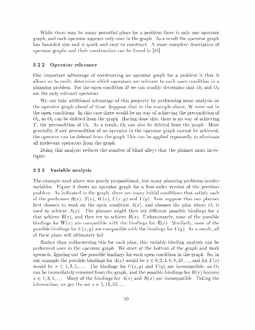
3.2.2 Operator relevance
One important advantage of constructing an operator graph for a problem is that it
allows us to easily determine which operators are relevant to each open condition in a
planning problem. For the open condition B we can readily determine that O3 and O4
are the only relevant operators.
We can take additional advantage of this property by performing some analysis on
the operator graph ahead of time. Suppose that in the example above, W were not in
the open conditions. In this case there would be no way of achieving the precondition ofO5, so O5 can be deleted from the graph. Having done this, there is no way of achievingT , the precondition of O3. As a result, O3 can also be deleted from the graph. Moregenerally, if any precondition of an operator in the operator graph cannot be achieved,
the operator can be deleted from the graph.This can be applied repeatedly to eliminateall irrelevant operators from the graph.
Doing this analysis reduces the number of blind alleys that the planner must inves-
tigate.
3.2.3 Variable analysis
The example used above was purely propositional, but many planning problems involvevariables. Figure 3 shows an operator graph for a �rst-order version of the previousproblem. As indicated in the graph, there are many initial conditions that satisfy eachof the predicates R(x), S(x), W (x), U(x; y) and V (y). Now suppose that our planner
�rst chooses to work on the open condition A(x), and chooses the plan where O1 isused to achieve A(x). The planner might then try di�erent possible bindings for xthat achieve R(x), and then try to achieve B(x). Unfortunately, none of the possible
bindings for W (x) are compatible with the bindings for R(x). Similarly, none of thepossible bindings for U(x; y) are compatible with the bindings for V (y). As a result, all
of these plans will ultimately fail.
Rather than rediscovering this for each plan, this variable binding analysis can be
performed once in the operator graph. We start at the bottom of the graph and work
upwards, �guring out the possible bindings for each open condition in the graph. So, inour example the possible bindings for A(x) would be x 2 0; 2; 4; 6; 8; 10 : : :, and for T (x)would be x 2 1; 3; 5; : : :. The bindings for U(x; y) and V (y) are incompatible, so O4
can be immediately removed from the graph, and the possible bindings for B(x) become
x 2 1; 3; 5; : : :. Many of the bindings for A(x) and B(x) are incompatible. Taking theintersection, we get the set x 2 5; 15; 25; : : :.
10

Finish
O1
A(x) B(x)
O2
S(x)R(x)
O3 O4
U(x,y)T(x) V(y)
O5
W(x)
x 2 4 6 …, , ,{ }∈ x 0 5 10 …, , ,{ }∈
x 1 3 5 …, , ,{ }∈
x 1 3 5 …, , ,{ }∈y 0= y 1 2 3 …, , ,{ }∈
Figure 3: First-order Operator graph.
11

Finish
A(x) B(x)
O2
S(x)
O3
T(x)
O5
W(x)
x 5 15 25 …, , ,{ }∈
x 5 15 25 …, , ,{ }∈
x 5 15 25 …, , ,{ }∈
x 5 15 25 …, , ,{ }∈
x 5 15 25 …, , ,{ }∈
Figure 4: Operator graph after variable analysis.
The second part of the process is to propagate these limitations back down the tree.When we do this for A(x) we �nd that the remaining bindings are incompatible with thebindings for R(x), so O1 can be deleted from the graph. When the process is complete,the resulting operator graph is as shown in Figure 4. This operator graph dramaticallylimits the space of plans that will have to be explored by the planner.
In general, variable analysis in the operator graph can be expensive because the sets ofvariable bindings can become large. However it is always possible to simplify the bindingsets by removing those variables that have too many possible solutions. Removing the
variable means that we are assuming it can take on any possible value. This may reduce
the amount of pruning that can be done, but doesn't a�ect the completeness or soundnessof the planning process.
3.2.4 Open condition ordering
The choice of which open condition to work on next often results in orders of magnitude
di�erence in the amount of search required. The most important factor in deciding which
open condition to work on next is the number of di�erent possible ways of achieving theopen condition. If there are few potential plans for an open condition, then choosing
and expanding that open condition does not signi�cantly increase the number of partialplans. Alternatively, expanding an open condition with many options leads to many
12

possible plans.
Counting the number of possible expansions for each open condition does add over-
head to the planning process. However, the operator graph can be used to help speed
this process. First, it provides an upper bound on the number of possibilities for each
open condition. Second, it allows the planner to rapidly �nd and count the relevant
expansions for each open condition. As a result, the overhead for this technique seems
to be minimal. We have evaluated this technique in several standard planning test do-
mains and found it to be extremely successful. These experimental results can be found
in [38]. Joslin [27] has done further evaluation of this technique and has con�rmed its
signi�cance.
3.2.5 Recursion analysis
Many operators in planning problems allow recursion. For example, a transportation
operator might be used to go from A to B, but might also be used to go back from B
to A. This means that a plan can be constructed that involves going back and forthbetween A and B any number of times. Sometimes this may be necessary. For example,several trips might be necessary to transport all the supplies to B. Unfortunately, suchoperators also allow planners to construct and investigate lots of ridiculous plans.
We've developed a technique that helps to avoid useless recursion. The basic idea isto recognize when the planner has generated a repeated subgoal and suspend work on
that subgoal until there is some other reason for exploring that repeated subgoal. Toillustrate, consider the partial plan in Figure 5a. The goal is to achieve P and R, andthe step S1 is used to achieve P . S2 is used to achieve the precondition Q of S1, but S2
has the precondition P , which is one of the goals the planner was trying to achieve in the�rst place. As a result, the open condition P of S2 can be suspended. This means thatthe planner should not work on this open condition unless some other open condition is
linked into either S1 or S2. In Figure 5b, the open condition R is now being establishedby S2. As a result, the condition P must be reenabled. In contrast, if no other opencondition is ever linked to S1 or S2 (as in Figure 5c), the plan is discarded.
There is considerable overhead involved in recognizing recursive open conditions, andin checking to see when they should be re-enabled. Operator graphs help considerablyin this process because they make it clear which open conditions are susceptible to
recursion, and also make it clear which operators could potentially link into a recursion
and cause open conditions to be re-enabled. (If there is no possibility of such links, theplan can be discarded early.)
There are a number of subtleties involved in the general technique.
1. The presence of variables makes suspension and enablement conditions more com-
plex.
2. Certain con icts between operators may also require re-enablement of suspended
open conditions.
13

Finish
S1
S2
P
Q
P
R
Finish
S1
S2
P
Q
P
R
(suspended) (re-enabled)
Finish
S1
S2
P
Q
P
R
(suspended)
S3
Figure 5: Partial plans with recursion.
A more complete description of this technique can be found in [40].
3.2.6 Postponing Con icts
During the planning process, con icts often arise between operators used to achievedi�erent parts of a goal. For example, one operator may consume a resource needed foranother operator, or may change some condition in the world that is a prerequisite foranother operator. Resolving these con icts is therefore a critical part of the planningprocess.
Several planners [39], [49], [50] ignore con icts until planning is otherwise complete,and then try to �x the plan to eliminate con icts. If the subgoals in the problem interact
only loosely, this can be an e�cient strategy. However, if there are complex interactions
between the subgoals and operators for a problem, this approach results in extensivebacktracking by the planner.
An alternative approach used in recent planning systems [31], [2], [52], [8] is to resolve
each con ict as it arises during the planning process. Using this approach a planner
notices unresolvable con icts early in the planning process. The problem is that there
are often many possible ways to resolve each con ict, thus contributing to an explosion
in the search space. More bluntly, resolving con icts during planning multiplies theexponential task of con ict resolution by the exponential task of planning.
Both of these alternatives are too extreme. Many con icts are simple to resolve andcan be delayed until the end. However, those that are tightly interconnected need to be
14
resolved during the planning process (once the entire group of con icts is generated). We
have developed techniques for automatically deciding which con icts should be resolved
during the planning process, and which con icts should be delayed until planning is oth-
erwise complete. The basic idea is to analyze the potential con icts between operators
in the operator graph. Roughly, a set of con icts can be postponed if we can show in the
operator graph that there will always be a way of eliminating the con icts by imposing
partial ordering constraints among the operators. Under these circumstances, the post-
poned con icts can be ignored during planning, and can always be resolved by imposing
additional ordering constraints on the otherwise complete plan. The technique is also
recursive; postponing one set of con icts may then allow postponing more con icts.
In loosely coupled domains, many of the con icts can usually be postponed. This has
the e�ect of decoupling the planning problem into two pieces: selection of the operators
for achieving the goals, and ordering the operators to eliminate con icts between them.
This can result in dramatic reductions in the amount of search required to �nd a plan.
More complete descriptions of this technique can be found in [43] and [44].
3.2.7 Con ict resolution strategies
Not all con icts can be postponed. In this case the question arises as to when con ictsshould be resolved during the planning process. The two options, resolve con icts im-
mediately, and resolve con icts at the end, represent two extreme positions. There areseveral other interesting options:
DSEP : Wait to resolve a con ict until the variable bindings guarantee that the con ict
will occur.
DUNF : Wait to resolve a con ict until there is only a single way of resolving it.
DRES : Continue checking each con ict to make sure it can be resolved, but don'tresolve con icts until the end.
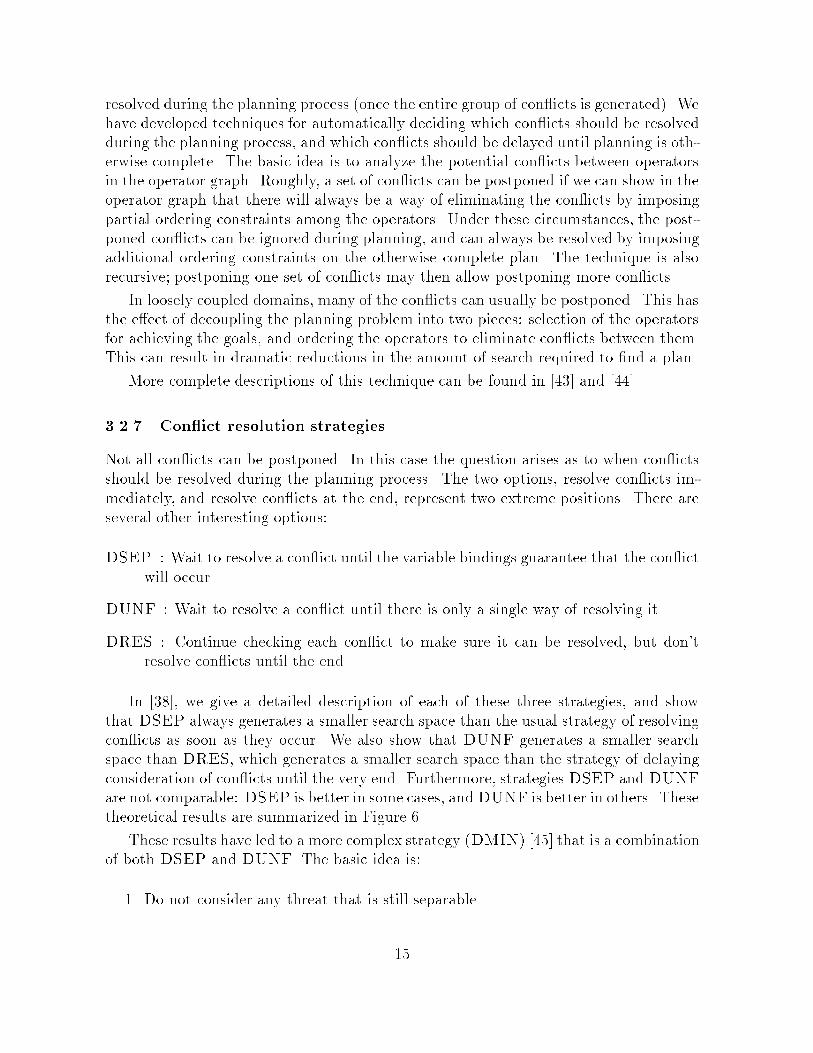
In [38], we give a detailed description of each of these three strategies, and showthat DSEP always generates a smaller search space than the usual strategy of resolvingcon icts as soon as they occur. We also show that DUNF generates a smaller search
space than DRES, which generates a smaller search space than the strategy of delaying
consideration of con icts until the very end. Furthermore, strategies DSEP and DUNFare not comparable: DSEP is better in some cases, andDUNF is better in others. These
theoretical results are summarized in Figure 6
These results have led to a more complex strategy (DMIN) [45] that is a combination
of both DSEP and DUNF. The basic idea is:
1. Do not consider any threat that is still separable.
15

Immediate
DSEP DUNF
DRES
Delay
Figure 6: Search space relationships for �ve threat removal strategies.
2. Resolve any threat that has only one possible resolution.
3. Verify that there is a way of resolving any remaining threats (not covered by 1 and2), but do not commit to any particular resolution of these threats.
We have shown, theoretically, that this combination strategy always generates a
search space that is the same size or smaller than that of either DSEP or DUNF.We have veri�ed all of these theoretical results by testing these strategies on severalstandard planning test domains. A complete description of these experiments can befound in [38]. Joslin, [27], and Kambhampati, [28], have also con�rmed several of theseexperimental results.
3.3 Partial Plan Evaluation
In general we want planners that �nd not just any plan, but a good plan. Given utilitymodels for a planning domain, we can evaluate and compare completed plans. However,it is computationally intractable to generate and compare all possible plans for a signif-
icant domain. Instead, we need to be able to evaluate and compare partial plans duringthe planning process, so that planning e�ort can be focused on the most \promising"plans. The tough part here is being able to estimate the cost and probability of suc-cess for those parts of the plan that are not yet complete. More precisely, we want to
know how much it will cost, and how likely it is that we can achieve the remaining open
conditions in the plan. This, together with the actions already in the plan, allows anestimate of the overall worth of the partial plan.
Operator graphs can be used to help estimate costs and probabilities for un�nished
parts of the plan. To see how this works, consider the operator graph in Figure 7, where
C1 through C5 are the costs of operators O1 through O5 respectively. According to the
operator graph, the conditions R, S, W , U , and V can all be satis�ed by the initialconditions. As a result, they would all have cost 0. Next consider the condition A.
There are two possible operators that can be used to achieve A, O1, and O2. If O1 is
used, a cost of C1 will be incurred, plus the cost of achieving O1's preconditions. If O2 is
16

Finish
O1
A B
O2
SR
O3 O4
UT V
O5
W
C1 C2 C3 C4
C5
Figure 7: Propositional operator graph with operator costs.
used, a cost of C2 will be incurred, plus the cost of achieving O2's preconditions. Thusthe best we can expect for achieving A is the minimum of these two costs, min(C1; C2).Similarly, the best we can expect for achieving B is min(C3 + C5; C4).
Now consider the partial plan shown in Figure 8. It contains one step, an instanceof O2, and two open conditions, S, and B. The cost of O2 is C2, the cost for S is 0, andthe best cost for B is min(C3+C5; C4). As a result, the best cost for this partial plan isC2+min(C3+C5; C4). Using this cost, this plan can be compared with other candidatepartial plans.
In the above example, our calculations were particularly simple because the operatorsare all propositional (no variables) and there is no recursion possible. When variablesand/or recursion are present, the analysis becomes much more complex. For example,
when variables are present, the cost of achieving a particular open condition may depend
heavily on the variable bindings. To take this into account we must use variable analysislike that described in Section 3.2.3 to �nd out the possible relevant bindings for variables.
We then compute minimumcosts for these di�erent possible variable bindings. Recursionamong the operators poses similar problems.
Although we only considered cost in this example, the same kind of calculations can
be done for probability of success and utility. The key is that the operator graph allowsus to consider the alternative ways of achieving each potential subgoal, to facilitate some
17

Finish
A B
O2
S
C2
Figure 8: Partial plan with two open conditions.
estimate of how costly it will be to achieve that subgoal.
A more detailed description of this ongoing work can be found in [41].
4 Plan Evaluation
For plan evaluation, Rockwell e�orts concentrated on the building of utility models, and
the use of both in-house tools (IDEAL and IDEAL-DEMOS [48, 46]) and commercialtools (DEMOS [51]) for decision making and inference. The �rst signi�cant productof this e�ort was the Transportation Trade-o� Analyzer (TTA). This was a decision-theoretic based tool that demonstrated substantial capability enhancements over tra-ditional transportation schedulers and feasibility estimators. The TTA is described in
Section 4.1 and in previous annual reports to ARPI [4, 3].
The TTA was demonstrated at the end of the �rst year of the program, and as aresult, Rockwell was invited to apply these decision-theoretic tools to the crisis action
planning domain for the Third Integrated Feasibility Demonstration (IFD-3). Rockwell,along with ISX, developed the Course Of Action Trade-o� Analyzer (COATA) for Non-
combatant Evacuation Operations. The functionality provided by COATA was well
received by the Operational Planning Team at the U.S. Paci�c Command, and COATAwas showcased in the original version of TARGET developed for IFD-3 as one of only
a handful of Planning Initiative technologies then present in TARGET. On the basis ofthe work on COATA, Rockwell was invited to be a member of BBN's successful bid for
the Deployable Joint Task Force Advanced Technology Program. COATA is describedin Section 4.3.
Rockwell made available two decision-theoretic tools to the Planning Initiative com-
18

Figure 9: Model structure used in the Transportation Trade-O� Analyzer.
munity through the CPE.1 These tools, IDEAL and IDEAL-DEMOS, are general decision-
theoretic modeling tools that can be applied to a wide range of tasks. IDEAL is currently
in use by hundreds of researchers within the decision theory and probabilistic reasoningcommunity. Section 4.2 brie y describes the capabilities of IDEAL and IDEAL-DEMOS;further information can be found in [47, 46].
Finally, the development of utility models for crisis management pointed to the need
for new techniques on sensitivity analysis, speci�cally on the computation of expectedvalue of information. The new techniques and algorithms developed by Rockwell for this
program are described in Section 4.4.
1Rockwell was in fact one of the �rst PI members to provide tools for other members.
19

4.1 Transportation Trade-o� Analyzer
As the ARPI began in 1991, the focus was on increasing the capabilities of DOD tools
for military transportation planning and scheduling. Our �rst goal was to explore the
domain of military transportation planning and to capture the essential uncertainties and
trade-o�s inherent in this domain. The strategy was to develop utility and value models
that express trade-o�s between consumption of resources and achievement of goals under
uncertainty, in order to express the preferences, objectives, and knowledge of DOD
planning commands. Once this was done, we encoded this information in a decision-
theoretic model which provided help with such capabilities as generating alternative
plans, guiding search, and controlling computational resource allocation.
The domain study included training at the Armed Forces Sta� College. The resulting
tool was named \Transportation Trade-o� Analyzer (TTA)". Uncertainty was modeled
explicitly using belief networks and in uence diagrams [32], and e�cient mechanismsfor reasoning with probabilistic information were employed. By explicitly modelingcosts, the e�ects of delay, and uncertainties in the transportation process, TTA is ableto optimize the transportation plan for changing requirements and under the changing
conditions of the real world. In its most basic con�guration, holding costs and resources�xed, the TTA model performs the same functionality as RAPIDSIM or DART in mea-suring plan feasibility. By relaxing these arti�cial constraints, TTA is able to providesigni�cantly enhanced information. The characteristics of the TTA model are describedin depth in Rockwell's �rst annual report [4]. A picture of the top level TTA screen is
shown in Figure 9.
4.2 Decision-Theoretic Modeling Tools in the CPE
After the �rst year of the PI program, Rockwell made two general decision-theoreticmodeling tools available to the other members of the PI community. These tools, IDEAL
and IDEAL-DEMOS [48, 47, 46], were placed in the Common Prototyping Environment(CPE), and were some of the �rst researcher-based tools to be made available there.
IDEAL is a LISP-based test bed for work in in uence diagrams and Bayesian net-
works. It contains various inference algorithms for belief networks and evaluation al-gorithms for in uence diagrams. It contains facilities for creating and editing in uencediagrams and belief networks both programmatically and via a CLIM-based graphical
editor called IDEAL-EDIT [17]. An IDEAL-EDIT window displaying a basic IDEAL
in uence diagram is shown below in Figure 10.
IDEAL-DEMOS is a LISP reimplementation of the core of the DEMOS [51] modeling
language. The objective was to complement the IDEAL inference system with some ofthe inference capabilities present in DEMOS.2
2DEMOS is a commercially available system for decision modeling.
20

Figure 10: An example of an in uence diagram in IDEAL-EDIT.
21

US
CIT
S a
t A
ssem
bly
Day0 2 4 6 8 1 0
0
5 0 0
1 0 0 0
1 5 0 0
2 0 0 0
Key Transport Force ChoiceC - 1 3 0 sC-141s and Chartered
Figure 11: The graph describes the buildup of U.S. citizens at an assembly area.
4.3 Course Of Action Trade-o� Analyzer
The success of the TTA model and the knowledge learned from its construction wasbene�cial in several ways. As well as providing feedback that was useful in other research
e�orts, Rockwell was invited to apply the same techniques used in the TTA model tothe domain of crisis action planning for the Third Integrated Feasibility Demonstration(IFD-3) of the ARPA/Rome Labs Planning Initiative. Rockwell provided the decision-theoretic plan evaluation capabilities for the Theater-level Analysis, Replanning and
Graphical Execution Toolbox (TARGET) during IFD-3. These capabilities included the
means of estimating the feasibility, costs, casualties, and times associated with variouscourses of actions (COA). The targeted user was the executive o�cer of the Opera-
tional Planning Team (OPT). The objective was to provide a computational tool, called\Course of Action Trade-o� Analyzer" (COATA), for capturing the assumptions and the
rationale behind the planning process. The output of COATA is a set of estimates andentries that can support the development of a COA selection matrix. Figure 11 shows
an example of these outputs.
COATA consists of three components: a decision model, an inference engine, and a
graphical interface. The decision model was developed by Rockwell personnel in con-
junction with U.S. Paci�c Command to support COA analysis for Non-combatant Evac-
22

AircraftPerformance
In Country toAssembly Area
Transfer
NEOCourse
of ActionAlternatives
Assembly Areato Safe Haven
Transfer
TotalEstimatedAMCITSAttrition
NEO Transferto Safe Haven
Profile
UncertaintyAnalysis
Inputs andAssumptions
In CountryEstimated
Attrition
Assembly Area Estimated
Attrition
DatabaseInformation
COA Selection
Matrix
Security ForceTransfer toAssembly
Figure 12: Top level model for the NEO course of action analysis tool. The tool generates
graphs describing risks for U.S. citizens and estimates of transportation times.
23

uation Operations (NEO). The inference engine is part of a Rockwell in-house tool for
decision making under uncertainty, and the run-time graphical interface was developed
primarily by ISX.
The model assumes the following scenario: A situation arises which requires the
evacuation of U.S. civilians from a foreign country. These U.S. citizens, located in one
or more regions in the host country, are told to move from their current locations to
one or more assembly areas in the country. Simultaneously, U.S. military forces are
deployed from their current locations in the world to the assembly areas. Upon arrival,
the military forces secure the assembly areas for civilian transit. Transportation assets
are utilized to move the U.S. citizens from the assembly areas to safe haven(s), which
are generally located outside of the country. The top level model (in the form of an
in uence diagram) is shown in Figure 12.
The COATA model allows the user to instantiate a generic NEO plan with speci�c
locations, forces, and destinations, along with the (possible) uncertainties associatedwith this information (represented by probability distributions), and then to performtrade-o� analyses for di�erent courses of action. The user or some other automatedplanner must specify the speci�c data regarding country locations and number of citizens,
the assembly areas, safe havens, security forces, and transportation assets. In addition,estimates on the risk to the U.S. citizens and the military of attrition (death) at variousstages of the operation are also needed. The di�erent COAs are de�ned by the choiceof security forces (including their original location, date of availability and capabilities),safe havens, and transportation assets. Note that the use of probability distributions
allows the speci�cation of uncertain and incomplete data that can be re�ned during thevarious stages of the planning process.
Once the necessary information is speci�ed, the model performs a dynamic simulation
of the ow of U.S. citizens from their initial locations to assembly areas and then tothe safe havens. Some of the more important outputs of the model include: time tocompletion, total of U.S. civilian and military casualties, speed of �rst response, andmaximum build-up of U.S. citizens at assembly areas. The model also includes riskfactors associated with both U.S. citizens and U.S. military personnel as a function of
time. These risk factors are used to calculate expected casualties for various options.Additionally, since the uncertainty of any input is represented in the model, the tool is
capable of generating an expected value for the parameter as well as a full uncertainty
distribution for any of the output parameters.
The COATA tool provided a successful demonstration of technology transfer for
IFD-3 at PACOM in May and September of 1993. The senior o�cer for the OPT atPACOM, who helped to develop the model, gave high marks to the capabilities of the
tool. Currently, the Rockwell Palo Alto Laboratory is a member of an on-going project
to extend the TARGET capabilities to the deployable Joint Task Force. The secondannual report contains more speci�c information about COATA [3].
24

4.4 Sensitivity Analysis in Planning
The experience in building computer-based utility models for evaluating and simulating
crisis scenarios pointed towards the need for more sophisticated techniques and methods
for sensitivity analysis. It is necessary to decide which aspects of a scenario are essential
for planning and need to be represented in the model, and which aspects can be ignored.
The reason is simple: given that information is an expensive commodity, every model
must balance the desire for maximumprecision and detail against the need to get the job
done with limited time, data, and computational resources. This tension is particularly
acute in military crisis planning, where the stakes, risks and complexities are typically
high, and where the deadlines are always tight.
Decision theory, and the techniques of decision analysis that are based on it, provide
a number of powerful methods for analyzing these trade-o�s between the precision of a
model and the resources required to analyze it. The explicit representation of uncertaintyin the form of probability distributions allows comparison of the e�ects of the di�erentsources of uncertainty, and analysis of the costs and bene�ts of obtaining more detailedinformation to reduce the uncertainty. A planner needs to know which uncertainties
matter, but he or she also needs to know how to allocate economic resources to resolveor reduce those uncertainties.
We have therefore focused on giving planners tools for sensitivity analysis and
scenario management. Faced with dozens, possibly hundreds, of variables, with com-plex interdependencies and interactions among them, planners need principled, e�cienttechniques for identifying the most relevant or essential factors. They need to knowwhere their strategies are most likely to "break," and, in particular, what uncertaintiescontribute most to the fragility of their plans. Such knowledge, in turn, helps them allo-
cate resources (e.g., deployment of intelligence assets, consultation with other experts)for information-gathering and uncertainty/risk reduction.
For example, consider the NEO-COA model, developed by the Rockwell Palo Alto
Laboratory, in collaboration with planners from PACOM, the Paci�c Crisis Planningteam introduced in Section 4.3, and described in [3]. NEO-COA was designed to helpmilitary planners analyze alternate courses of action for the evacuation of U.S. citizensfrom crisis areas. Examples of uncertainties explicitly represented in NEO-COA are the
numbers of U.S. citizens, their locations in particular crisis regions, the accumulated
risks they face over time, and the rates at which they move to assembly areas andpoints of embarcation. The number of citizens in the capital might be a probability
distribution with median 500, and a 90% probability that the total is between 300 and1000. Should planners go ahead now and schedule air transports with capacity for, say,
1000 evacuees? Should they wait until intelligence provides a more precise estimate? Or
should they schedule air transports to carry 500 evacuees, with further capacity 500 tobe held in reserve? NEO-COA can help planners compare these alternatives, and assess
the expected value of better information relative to the costs of waiting for it.
25

4.4.1 The Expected Value of Information
The Expected Value of Information (EVI) is the best sensitivity measure because it
analyzes a variable's importance in terms of the recommended action, and it expresses
that importance in the value units of the problem. Other methods, such as rank-order
correlation, measure a variable's contribution to the overall uncertainty in the model's
outputs, expressed as a probability correlation. EVI, in contrast, measures a variable's
importance in terms of what matters | in the case of NEO-COA, for example, civilian
lives.
Certain methods, such as deterministic perturbation, measure a variable's impor-
tance in terms of what matters; yet they can still mislead. For example, suppose the
only available evacuation transport is a ship that can hold 1500 passengers, and the key
plan option is the choice of safe haven. The number of U.S. citizens at risk in the crisis
region may a�ect the overall outcome of the operation, but will probably not a�ect theplan choice. EVI would reveal uncertainty about the number of evacuees to be irrelevantto the plan choice, while deterministic perturbation might show high sensitivity to thisvariable.
The use of less powerful sensitivity measures can mislead planners into thinking thatit is worthwhile to wait for information about variables which are, in fact, irrelevant.Such sensitivities re ect the potential of new information to change beliefs or values
on outcomes. EVI, in contrast, measures the potential of new information to changedecisions.
4.4.2 Computing the Value of Information in Large Decision Models
To date, calculation of EVI has remained largely intractable for models of any reasonablesize. In models with discrete variables (i.e., models that admit solutions using decisiontrees), EVI has computational complexity that is exponential in the number of state
variables. For models with continuous variables such as NEO-COA, there were, to ourknowledge, no algorithms | exponential or otherwise | for calculating EVI. Thus, animportant part of our work has been to develop e�cient methods for calculating EVI inprobabilistic models for planning.
The innovative approach we developed is based on three features: The synthesis of
an initial high dimensional problem into a summarizing function, the introduction ofspecial information measures, and an e�cient pre-posterior analysis. The algorithmic
techniques are conceptualized in Figure 13, and a precise description of the algorithm
and the results of its application to NEO can be found in [6, 7].
D denotes a set of m mutually exclusive actions; X is a vector of n state variables,
all of which may be de�ned as probability distributions. The set-up alone makes clear
why the calculation of EVI is di�cult: it is a high-dimensional problem; worse, each
dimension is itself a random variable. We assume a value function V (d;X), whichspeci�es value to the decision maker when X assumes a particular value and action d
26

Figure 13: Conceptual overview of the algorithm for estimating EVI.
has been taken. Formally, the de�nition of EVI is as follows:
EV I = maxd
E[V (d;X)jX; s] �maxd
E[V (d;X)js] (1)
where E denotes expectation and s stands for the decision maker's prior state of infor-mation. (We include s simply to emphasize that all the quantities in the model have
been assessed relative to the decision maker's prior state of information.) That is, EVI isthe di�erence in expected value achieved by taking the optimal action with informationon X, and the optimal action without information on X. For simplicity, in what follows
we assume that D consists of just two discrete actions, d1 and d2.
Observing Figure 13, we see that X and D are applied as inputs to a linearizing
method to be described shortly; the output is a variable we call Z. Z is de�ned as thedi�erence in value between d2 and d1, assuming that d2 is the preferred action (i.e., d2yields higher expected value than d1).
Z = V (X; d2)� V (X; d1): (2)
In Figure 14, we show a graph of the probability distribution for Z.
Z is the pivotal element of our analysis because it essentially collapses the dimen-sionality of our original problem. We begin with n probability distributions for each
of the variables of X, a separate set of actions D, and a value function V (X; d). The
27

Figure 14: Probability distribution on Z.
probability distribution on Z | a simpler, two-dimensional quantity | encodes all theinformation from these elements that is vital for calculating EVI.
For the next portion of the analysis we consider the impact of evidence or informatione on any of the state variables in X. We use two measures, ESS (equivalent sample size)and RIM (relative information multiple) to describe the magnitude of new information.ESS is commonly used in statistical decision theory; RIM is a new measure we have
introduced. If X is the variable about which we expect to receive new information,then ESS is an equivalent number of observations on X's value, while RIM speci�es areduction factor in the variance of the probability distribution for X. The advantage ofa RIM is that it is de�ned in terms of a parameter already familiar to the decision maker| the variance of the probability distribution for X. In essence, these measures allow
the user to calculate the value of gathering more information about a certain variable,
where \more" is formalized as a multiplicative factor of the initial state of uncertainty:e.g., what would be the value of decreasing by a factor of 2 our uncertainty on the exactnumber of citizens in the capital?
The �nal step of the analysis requires preposterior analysis on Z to calculate thee�ects of e, expressed in RIM's or ESS, on combinations of state variables. We rely
on our linearizing method, probabilistic analysis, and numerical techniques to solve forEVI.
We have applied the algorithm to a large-scale decision model for planning NEO-COAintroduced in Section 4.3. The results are described in [6, 7], and include:
� an operational framework for calculating EVI based on ideas from statistical deci-
28

sion theory;
� an e�cient approximation algorithm for EVI;
� a formal analysis which guarantees the convergence of the algorithm, using a stop-
ping rule which tests a simple condition involving pre-speci�ed error parameters
and the algorithm's current estimate; in addition, a guarantee that the algorithm's
estimate is "probably approximately correct" | that is, with probability at least
1� �, the algorithm's output is within relative error " of the "true" answer.
� a knowledge representation for evidence or information that accommodates per-
fect/partial EVI;
� an application of the algorithm to the NEO-COA model; and
� implementation of the algorithm in detachable software modules using DEMOS [51],a commercially available software tool.
In addition, we have recently completed a set of experiments demonstrating thatthe algorithm is stable in the sense that, as its running time increases, its estimatesconverge at roughly the same rate as answers calculated using exact techniques. Wehave veri�ed that, while the linearizing assumption introduces error, its errors are at
least well-behaved compared to the errors introduced by any estimation algorithm. Thisis important, because we want to insure that the errors in the algorithm's outputs areat least systematic, and that they decrease monotonically as we increase the algorithm'srunning time.
Our immediate goal is to apply the resulting algorithm to other large probabilisticmodels for planning. We are especially interested to see how well it "scales up" in large,temporal models for planning under uncertainty, though we do not anticipate di�cultieswith such an application.
In sum, we have developed, implemented and tested an e�cient algorithm for
anytime approximation of EVI in large probabilistic models, for perfect and/orpartial information on any combination of variables, and with no limiting assumptions
about the distributions of the variables, the nature of the value function, or the numberof possible actions.
5 Plan Simulation
Our work on plan simulation was directed towards creating a tool for supporting the
functionality portrayed in Figure 15. Here, a human planner is confronted with a sit-
uation, an objective and some courses of action (plans) that are believed to achievethe objective. The human planner, however, is looking for assistance in simulating the
behavior of each of these plans to make a choice on which one to adopt. The purpose of
29

Action NetworksAction Networks
Simulation/AnalysisQueries
A Suiteof Plans
DomainModels
Iterative Feedback
Action Networks
Plan Simulator & Analyzer
Figure 15: Schematic view of a plan simulation scenario.
our work under this part of the contract is to develop such a tool, which is comprised oftwo major components:
1. A language for modeling the situation at hand.
2. A set of algorithms that operate on the model in order to simulate a plan.
These two components are described in the following two sections (Sections 5.1 and 5.2.
5.1 Action Networks
The �rst step in simulating and analyzing a plan is to describe the domain in which
this plan will be executed. According to the terminology used in SWAT team B report,
this amounts to creating a situation model. In our research program, we proposed the
30

formalism of action networks to construct a situation model and used them to simulate
military plans (see Figure 16). In the remainder of this section, we will focus on the
following:
1. Provide a brief introduction into action networks as a domain modeling language
2. Summarize the current status of action networks based on research conducted
under this contract
5.1.1 Introduction into action networks
An action network is a modeling tool oriented mainly towards dynamic domains that can
be controlled by agents. Action networks are very closely connected to what is known
as causal networks, which are the most sophisticated and e�ective tools for modeling
domains under uncertainty as demonstrated by many real-world applications [5, 32].
The di�erence between (the recently developed) action networks and (the by now
matured) causal networks is that causal networks do not include explicit constructs formodeling time and action, which are the key primitives for generating plans in dynamicdomains. Our work on action networks was aimed mainly on introducing these twoprimitives to causal networks. We emphasize here that each action network is equivalentto a causal network. Therefore, action networks are supported by all the theoreticaland practical tools that have been developed for causal networks, including the theory
developed in [32] and the various commercial tools available from a number of vendors.
5.1.2 Progress on Action Networks
The �rst publication on action networks appeared in [14], which describes the followingadditions that action networks brought to causal networks:
1. Controllable variables (action), which are variables in a causal structure that canbe controlled by agents. With respect to a controllable variable, an action net-
work may designate a number of other variables that determine the conditions of
controllability. These are called precondition variables and are connected to thecontrollable variables using a precondition arc.
2. Persistent variables (facts), which are variables in a causal structure the values of
which persists over time unless acted upon by agents.
Variables that are neither actions nor facts are called events. These are variables thatcannot be controlled but at the same time will retain their values over time.
In terms of implementational details, action networks and a number of corresponding
inference algorithms are implemented in C-NETS [11], a common lisp system of which
we are constructing a C version.
31

Rebel Threatin Abyss
Rebel Threat in Delta
Troops Location
Civilians at AA
Successful arrival to Delta
Civilians on their way to Delta
Planes Availability
Rebel Forest Access
Figure 16: An example of an action network.
32

In addition to controllable and persistent variables, action networks have brought
to traditional causal networks the ability do symbolic and qualitative reasoning under
uncertainty. Traditionally, causal networks have been probabilistic in the sense that
cause{e�ect interactions are quanti�ed by providing probabilities of e�ects given their
causes. But action networks are not necessarily probabilistic. Instead, a causal network
will consist of two parts: a directed graph � representing a \blueprint" of the causal rela-
tionships in the domain and a quanti�cation Q of these relationships. The quanti�cation
Q introduces a representation of the uncertainty in the domain because it speci�es the
degree to which causes will bring about their e�ects. Action networks allow uncertainty
to be speci�ed at di�erent levels of abstraction:
1. Point probabilities, which is the common practice in causal networks [32].
2. Order{of{magnitude probabilities, also known as epsilon probabilities [23, 24, 15].
One should emphasize here that causal networks are usually associated with proba-bilistic reasoning and therefore are perceived to inherit the problems associated with this
mode of reasoning, especially the infamous where-do-the-numbers-come-from? problem.We stress, however, that causal networks upon which action networks are based couldbe purely symbolic if the user so desires [16]. The principal investigators in this programhave been leading the e�orts for going beyond point probabilities in quantifying causalnetworks; their work on this can be found elsewhere [9, 23].
Although action networks support order-of-magnitude probabilities, they do not sup-port pure symbolic modeling yet. We plan to address this ability, however, in futureresearch.
5.2 Algorithms
5.2.1 Introduction
In our approach, plan simulation reduces computationally to reasoning with a belief
network. There is a number of algorithms in the literature for this purpose [32], but they
do perform poorly on networks generated for plan evaluation. The basic problem is theexistence of undirected cycles (loops) in the network, which complicates the computationprocess.3 Networks generated for plan evaluation tend to have many loops given their
temporal nature. For example, a network with one loop could have more than twenty
loops when expanded over three time steps.
To deal with networks containing loops, researchers have appealed to two concepts:
clustering and conditioning. In clustering, the network is aggregated to allow the de-composition of computations into simpler ones. In conditioning, certain variables are
instantiated to allow for conditional independences to hold, thus leading to more e�cient
3If no loops exist, the network is singly{connected and the computational complexity is linear in thenumber of nodes and arcs.
33

computations. The method of clustering is due to Lauritzen and Spiegelhalter [30], and
the conditioning algorithm is due to Pearl [32].
As was observed by Pearl [32], the use of conditioning to facilitate the computation
of beliefs is not foreign to human reasoning. When we �nd it hard to assess our belief
in a proposition, we often make hypothetical assumptions that render the assessment
simpler. This correspondence to human reasoning is probably the reason why cutset
conditioning was �rst expected to be more e�cient than other methods for evaluating
belief networks. But as observed later in [33], practice has shown that conditioning
turned out to be computationally less attractive than the Lauritzen and Spiegelhalter
algorithm [30].
Our commitment to conditioning methods stems from two factors: 1) We know that
we can apply these methods to any network independently of its quanti�cation [9],4 and
2) we have identi�ed a number of computational techniques that are best embedded
in the context of a conditioning method. To provide a set-up for implementing thesetechniques, we developed the method of dynamic conditioning, which is a re�nement of
cutset conditioning that makes it comparable in computational performance to cluster-ing methods. Based on dynamic conditioning, we developed the method of �-boundedconditioning, which is an approximate method that allows one to trade e�ciency foraccuracy of computation. We also investigated two specialized algorithms. The �rstis a prediction algorithm that applies to action networks only by taking advantage of
the recurrent structure of the temporal expansion of the action network. The secondalgorithm is also for prediction and is applied to order-of-magnitude networks only bytaking advantage of approximating probabilistic uncertainty to orders-of-magnitude un-certainty. We will discuss each of these algorithms in the following sections. But we�rst summarize the algorithms according to the properties that make them of interest
to plan simulation:
Dynamic Conditioning: A method for the exact simulation of plans and is based
on hypothetical reasoning (reasoning by cases). The signi�cance of the algorithmstems from: (1) It is the basis for the algorithm of �-bounded conditioning tobe discussed next; and (2) It is an infra-structure for realizing computational
techniques that are based on reasoning by cases.
�-bounded conditioning: A method for the approximate simulation of plans whichallows one to trade the exactness of the simulation with the time it takes to com-
pute the simulation. The signi�cance of this algorithm stems from the following
observation: Although the results of a particular simulation may not be exact,they may be enough to support a speci�c judgment about some plan.
Action Network Predict: An algorithm for predicting the e�ect of plans with respect
to a subclass of action networks. The algorithm has a polynomial computationalcomplexity on this subclass.
4To the best of our knowledge, there are no current results (or implementation) that suggests thatclustering methods can work for quanti�cations other than probabilistic.
34

PSA
User selects from a suite of algorithms, trading off speed for accuracy
User provides a set of courses of action to be simulated
Action Network, provided by the user, is a static description of the domain. It is automatically expanded over time in the PSA
Degree of Belief on: Successful arrival? Rebel threat? Civilians location? etc.
Figure 17: Current realization of the Plan Simulator and Analyzer (PSA) tool.
Kappa Predict: An algorithm for predicting the e�ect of plans with respect to order-of-magnitude action networks. The algorithm has a polynomial computational
complexity but may be unable to provide complete answers in certain cases. Thesigni�cance of this algorithm stems from at least two factors: (1) Although theanswers it provides may be incomplete, they may be enough to judge the qualityof given plans; and (2) It is a major building block of �-bounded conditioning thatwe discussed earlier.
Figure 17 shows a re�nement of the schematics in Figure 15, with a precise charac-terization of inputs and outputs including a choice of the algorithms described above for
computation.
5.2.2 Dynamic Conditioning
As a �rst step in our research on algorithms, we have attempted to show that condi-tioning methods can be as e�cient as clustering methods, thus setting the ground for
our further improvements on this approach. In particular, we re�ned cutset condition-
ing into the method of dynamic conditionining [12], which was shown experimentally toperform comparably to the Lauritzen and Spiegelhalter clustering method.
The breakthrough that permitted our results is the discovery of two important no-
tions in connection to conditioning methods: local and relevant cutsets, which are subsetsof a loop cutset on which the method of conditioning is based. Relevant cutsets can be
35

identi�ed in linear time and they usually lead to exponential savings when computing
beliefs in the light of assumptions. Local cutsets, on the other hand, eliminate the need
for considering an exponential number of assumptions because they identify assumptions
that lead to the same beliefs. Local cutsets can be computed in polynomial time from
relevant cutsets. The algorithm of dynamic conditioning is a re�nement of cutset con-
ditioning utilizing the notions of relevant and local cutsets. We provided experimental
results in [12] showing that dynamic conditioning performs comparably to the Lauritzen
and Spiegelhalter algorithm as implemented in IDEAL [19, 48]. We also discussed net-
work structures on which dynamic conditioning has a linear computational complexity,
while cutset conditioning leads to an exponential behavior.
Dynamic conditioning has been implemented in C-NETS [11]5 and tested for cor-
rectness against IDEAL [48] over hundreds of randomly generated networks.
5.2.3 Prediction Algorithm: Speci�c to action networks
Temporal causal networks that result from expanding atemporal networks (using thesuppressor model) [14] tend to have a large number of undirected cycles. These cycles
lead to networks that are di�cult to manage computationally; in fact, inference in suchnetworks is known to be NP-hard.
To deal with such networks, we have been exploring a number of approaches. One of
these approaches tries to prove independence properties about temporal networks thatare then utilized by algorithms in decomposing complex computations into simpler onesthat can be performed in parallel. A second approach explores task-speci�c procedureswith computation of approximate answers sacri�cing accuracy in order to gain speed.
A key result obtained under this investigation is that temporal networks that resultfrom expanding singly connected atemporal networks (without cycles) have some strongindependences properties. In particular, it can be shown that the parents �(Nt) of anynode Nt at time t become independent given the images of Nt and �(Nt) at time t� 1.
This independence is strong enough to justify the derivation of a sound and complete
algorithm for prediction that is linear in the number of time steps and exponentialonly in twice the number of parents per node. The algorithm is valid for inference inprobabilistic, kappa, and symbolic causal networks.
We stress here that although the original atemporal network may be singly connected,
its temporal expansion may have many cycles, which makes it very di�cult for generalpurpose inference algorithms. But by virtue of the expansion method (according to the
suppressor model), the resulting multiply connected network is guaranteed to satisfy
some strong independence properties.
5C-NETS is an environment for representing and computing with generalized causal networks [9, 13].Therefore, dynamic conditioning is not restricted to reasoning with probabilistic causal networks, butis also applicable to other classes of networks, such as kappa causal networks [21] and symbolic causalnetworks [10].
36

5.2.4 Prediction Algorithm: Speci�c to order-of-magnitude networks
The second approach we investigated is an algorithm for prediction that takes as input
a network quanti�ed with kappas (degrees of plausibility based on probabilities) and
returns as output the most plausible state of each variable.
The algorithm has the following properties:
1. The asymptotic complexity is O(max[E;N �LU]) where E is the number of edges
in the network, N is the number of nodes, and LU are table look-up operations.6
2. The algorithm is sound: If the algorithm predicts that x is the most plausible state
of X, then the probability of X = x is arbitrarily high.
3. The algorithm is complete only in any of the following cases:
� The matrices representing plausibility of nodes never leaves that plausibilityundetermined. That is for every state of the parents of the node in the
network there is a unique most plausible state.
� Nodes whose most plausible state remain uncommitted are not involved in
cycles where all other nodes are also uncommitted.
In the context of the algorithm, completeness means that if the probability ofX = x is high, then the algorithm should return x as the most plausible state of X.The lack of completeness simply means that some times the algorithm will remain
uncommitted regarding to the most plausible state of a variable X, even thoughthis state could be determined by exact (but time consuming) computations. Wepoint out that checking whether the result of a run of the algorithm for a speci�cquery is complete, is O(E) where E is the number of edges in the network.
This algorithm can be used to perform prediction, given a course of action, in a domainrepresented using default rules, or as an approximate prediction algorithm in proba-bilistic representation. The approximation is done as proposed in [15], by transformingexact probabilistic statements into order-of-magnitude probabilistic statements. Details
about the algorithm can be found in [22].
This algorithm is implemented on top of C-NETS [11].
5.2.5 Bounded Conditioning
�-bounded conditioning is a method for the approximate updating of causal networks.
It is a special case of bounded conditioning [26], which ranks the conditioning cases incutset conditioning according to their probabilities and then considers the more likely
cases �rst. The contribution of �-bounded conditioning is in:
6The uncertainty in the domain is stored in matrices associated with the nodes in a network. Atable look-up operation implies, in the worst case, examining all the entries of a particular matrix. Thesize of these matrices is nevertheless, bounded.
37

1. proposing a particular method for ranking the conditioning cases and
2. providing some guarantees about the approximate degrees of belief it computes.
To simplify the discussion, we will ignore the existence of evidence, therefore focusing
only on the computation of Pr(x) where X is a variable in the causal network.
Cutset conditioning computes the following sum [35],
Pr(x) =X
s
Pr(x ^ s);
where s ranges over all possible states of a loop cutset. The problem with cutset con-
ditioning, however, is that the number of cutset states is exponential in the size of the
cutset. To deal with this di�culty, bounded conditioning [26] orders the elements of the
above sum according to their values so that elements of a bigger value are considered�rst.
�-bounded conditioning splits members of the above sum into two classes, thoseexceeding a particular value � and those having a lesser or equal value to �. It thenignores the latter elements of the sum.
�-bounded conditioning applies to both probabilistic and kappa causal networks, butwe restrict the discussion here to probabilistic networks.
The Probabilistic Case
For some �, �-bounded conditioning splits the conditioning sum as follows:
Pr(x) =X
s;Pr(s)>�
Pr(x ^ s) +X
s;Pr(s)��
Pr(x ^ s):
The algorithm then ignoresP
s;Pr(s)�� Pr(x ^ s), thus computing:
Pr 0(x) =X
s;Pr(s)>�
Pr(x ^ s):
An important property of �-bounded conditioning is that we can judge the quality of
its approximations without knowing what the chosen value of � because it provides an
upper and a lower bound on the exact probability.
To completely specify �-bounded conditioning, we need to show how to identify cutset
states that have probability no more than �, which is discussed next.
Suppose that we have an algorithm such that for each variable X and value x it
will tell us whether Pr(x) � �. Using such an algorithm, call it �-algorithm, we can
identify all cutset states that have probabilities no more than an �. One such an �-
algorithm for prediction is the one we discussed earlier for order-of-magnitude networks.
This algorithm, which is linear in the number of arcs, is sound but incomplete, whereincompleteness means that the algorithm may return \unknown" for whether Pr(x) � �.
38

This incompleteness, however, does not matter for �-bounded conditioning: it only means
that some cutset states which have probability greater than � are being considered by �-
bounded conditioning although they should be ignored. Of course, however, the closer to
being complete the �-algorithm is, the better the performance of �-bounded conditioning
will be.
6 Concluding Remarks
Military planning activities, like most complex problems, must respond to multiple com-
peting objectives with uncertainty about actual outcomes. The approach pursued at the
Rockwell Science Center is centered on well founded normative notions of rational deci-
sion making and probability theory, and is based on the expertise of the researchers of
the laboratory in this area.
The results of this program, as summarized in Tables 1 and 2, have produced im-
portant advances in the state of the art in the generation, evaluation, and simulation ofplans, with recognized impact in both the scienti�c and application oriented communityas well as in ARPA. Moreover, we are currently investigating the application (and transi-tion) of the methods and technology developed under this program to Rockwell businessdivisions in the areas of automatic diagnosis, optimal repair, and resource allocation.
References
[1] A. Balke and J. Pearl. Probabilistic evaluation of counterfactual queries. In Pro-
ceedings of the 10th Conference on Uncertainty in Arti�cial, Intelligence, 1994. In
press.
[2] Anthony Barrett and Daniel S. Weld. Partial-order planning: evaluating possible
e�ciency gains. Arti�cial Intelligence, 67(1):71{112, 1994.
[3] John Breese, Michael Buckley, Tom Ch�avez, Max Henrion, Eric Horvitz, David
Smith, Mark Peot, and James White. Decision-theory for crisis management {
annual report II. Period of performance: February 1992 { January 1993, Contract
F30602-91-C-0031, 1993.
[4] John Breese, Max Henrion, David Smith, and Mark Peot. Decision-theory for crisismanagement { annual report I. Period of performance: February 1991 { January
1992, Contract F30602-91-C-0031, 1992.
[5] Eugene Charniak. Bayesian networks without tears. The AI Magazine, 12(4):50{63,
1991.
39

[6] Tom Ch�avez and Max Henrion. E�cient estimation of value of information in Monte
Carlo models. In Proceedings of the 10th Conference on Uncertainty in Arti�cial,
Intelligence, pages 119{127, 1994.
[7] Tom Ch�avez and Max Henrion. Focusing on what matters in plan evaluation:
E�ciently estimating the value of information. In Proceedings of the Workshop
of Knowledge Base Planning and Scheduling Initiative (ARPA{Rome Labs.), pages
387{400, 1994.
[8] Greg Collins and Louise Pryor. Achieving the functionality of �lter conditions in a
partial order planner. In Proceedings of the Tenth National Conference on Arti�cial
Intelligence, pages 375{380, 1992.
[9] Adnan Darwiche. A symbolic generalization of probability theory. PhD thesis, Com-
puter Science Dept., Stanford University, 1992.
[10] Adnan Darwiche. Argument calculus and networks. In Proceedings of the Ninth
Conference on Uncertainty in Arti�cial Intelligence, pages 420{421, WashingtonDC, 1993.
[11] Adnan Darwiche. CNETS: A computational environment for causal networks. Tech-nical memorandum, Rockwell International, Palo Alto Labs., 1994.
[12] Adnan Darwiche. Dynamic conditioning: An e�cient re�nement of cutset condi-tioning using local and relevant cutsets. Technical memorandum, Rockwell ScienceCenter, Palo Alto Labs., 1994.
[13] Adnan Darwiche and Matthew Ginsberg. A symbolic generalization of probabil-ity theory. In Proceedings of the American Association for Arti�cial Intelligence
Conference, pages 622{627, San Jose, CA, 1992.
[14] Adnan Darwiche and Mois�es Goldszmidt. Action networks: A framework for rea-soning about actions and change under uncertainty. In Proceedings of the 10th
Conference on Uncertainty in Arti�cial, Intelligence, pages 136{144, 1994.
[15] Adnan Darwiche and Mois�es Goldszmidt. On the relation between kappa calculus
and probabilistic reasoning. In Proceedings of the 10th Conference on Uncertainty
in Arti�cial, Intelligence, pages 145{153, 1994.
[16] Adnan Darwiche and Judea Pearl. Symbolic causal networks. In Proceedings of the
Twelfth National Conference on Arti�cial Intelligence, pages 238{244, 1994.
[17] Denise Draper and John Breese. IDEAL-EDIT: Documentation and user's guide.
Rockwell Science Center, Palo Alto Laboratory, 1992. Technical Memorandum #
77.
40

[18] Denise Draper, Steve Hanks, and Daniel Weld. Probabilistic planning with informa-
tion gathering and contingent execution. In Proceedings of the Second International
Conference on AI Planning Systems, pages 31{36, 1994.
[19] F.Jensen, S. Lauritzen, and K. Olesen. Bayesian updating in recursive graphical
models by local computations. Technical Report R 89-15, Institute for Electronic
Systems, Department of Mathematics and Computer Science, University of Aalborg,
Denmark, 1989.
[20] Robert P Goldman and Mark S. Boddy. Conditional linear planning. In Proceedings
of the Second International Conference on AI Planning Systems, pages 80{85, 1994.
[21] Mois�es Goldszmidt. Qualitative Probabilities: A Normative Framework for Com-
monsense Reasoning. PhD thesis, Computer Science Dept., University of California
Los Angeles, 1992. Technical Report TR-190, Cognitive Systems Laboratory.
[22] Mois�es Goldszmidt. Belief-based irrelevance and networks: Toward faster algo-rithms for prediction. Working notes: AAAI Fall Symposium on Relevance, 1994.
[23] Mois�es Goldszmidt and Judea Pearl. Rank-based systems: A simple approachto belief revision, belief update, and reasoning about evidence and actions. InPrinciples of Knowledge Representation and Reasoning: Proceedings of the Third
International Conference, pages 661{672, Boston, 1992.
[24] Mois�es Goldszmidt and Judea Pearl. Reasoning with qualitative probabilities canbe tractable. In Proceedings of the 8th Conference on Uncertainty in AI, pages112{120, Stanford, 1992.
[25] D. Heckerman, J. Breese, and K. Rommelse. Sequential troubleshooting under
uncertainty. Submitted to CACM, 1994.
[26] Eric Horvitz, Gregory Cooper, and H. Jacques Suerdmont. Bounded conditioning:Flexible inference for decisions under scarce resources. Technical Report KSL-89-42,Knowledge Systems Laboratory, Stanford University, 1989.
[27] David Joslin and Martha E. Pollack. Least-cost aw repair: a plan re�nement strat-
egy for partial-order planning. In Proceedings of the Twelfth National Conference
on Arti�cial Intelligence, pages 1004{1009, 1994.
[28] Subbarao Kamhampati, 1993. Personal communication.
[29] Subbarao Kamhampati, Craig Knoblock, and Qiang Yang. Planning as re�nementsearch: a uni�ed framework for evaluating design tradeo�s in partial order planning.
Arti�cial Intelligence, 1994. To appear.
[30] S. Lauritzen and D. Spiegelhalter. Local computations with probabilities on graph-
ical structures and their applications to expert systems. Royal Statistical Society,
50:154{227, 1988.
41

[31] David McAllester and David Rosenblitt. Systematic nonlinear planning. In Pro-
ceedings of the Ninth National Conference on Arti�cial Intelligence, pages 634{639,
1991.
[32] Judea Pearl. Probabilistic Reasoning in Intelligent Systems: Networks of Plausible
Inference. Morgan Kaufmann, San Mateo, CA, 1988.
[33] Judea Pearl. Belief networks revisited. Arti�cial Intelligence, Special Issue, \AI in
Perspective,"(59):49{56, 1993.
[34] J. Scott Penberthy and Daniel S. Weld. UCPOP: A sound, complete, partial order
planner for adl. In Proceedings of the Third International Conference on Knowledge
Representation and Reasoning, 1992.
[35] Mark Peot and Ross Shachter. Fusion and propagation with multiple observations
in belief networks. Journal of Arti�cial Intelligence, 48(3):299{318, 1991.
[36] Mark A. Peot. Decision-Theoretic Planning. PhD thesis, Stanford University, 1995.
In preparation.
[37] Mark A. Peot and David E. Smith. Conditional nonlinear planning. In Proceedings
of the First International Conference on AI Planning Systems, pages 189{197, 1992.
[38] Mark A. Peot and David E. Smith. Threat-removal strategies for partial-order plan-ning. In Proceedings of the Eleventh National Conference on Arti�cial Intelligence,
pages 492{499, 1993.
[39] Earl Sacerdoti. A structure for plans and behavior. North Holland, 1977.
[40] David E. Smith. Controlling recursion in planning. In preparation, 1994.
[41] David E. Smith. Evaluating partial plans. In preparation, 1994.
[42] David E. Smith and Mark A. Peot. A critical look at knoblock's hierachy mecha-
nism. In Proceedings of the First International Conference on AI Planning Systems,
pages 307{308, 1992.
[43] David E. Smith and Mark A. Peot. Postponing simple con icts in nonlinear plan-
ning. In Working Notes of the AAAI Spring Symposium on Foundations of Auto-
matic Planning: The Classical Approach and Beyond, pages 132{136, 1993.
[44] David E. Smith and Mark A. Peot. Postponing threats in partial-order planning.
In Proceedings of the Eleventh National Conference on Arti�cial Intelligence, pages500{506, 1993.
[45] David E. Smith and Mark A. Peot. A note on the dmin strategy. Available by
request, 1994.
42

[46] Sampath Srinivas. IDEAL-DEMOS: Documentation and user's guide. Rockwell
Science Center, Palo Alto Laboratory, 1992. Technical Memorandum # 76.
[47] Sampath Srinivas and John Breese. IDEAL: In uence diagram evaluation and
analysis in Lisp. Documentation and user's guide. Rockwell Science Center, Palo
Alto Laboratory, 1989. Technical Memorandum # 23.
[48] Sampath Srinivas and John Breese. IDEAL: a software package for analysis of
in uence diagrams. In Proceedings of the 6th Conference on Uncertainty in Arti�cial
Intelligence, Cambridge, MA, 1990.
[49] Gerald Sussman. A computational model of skill acquisition. Technical report, MIT
AI Laboratory, 1973.
[50] David E. Wilkins. Practical Pplanning: Extending the Classical AI Planning
Paradigm. Morgan Kau�man, 1988.
[51] NeilWishbow and Max Henrion. Demos User's Manual. Department of Engineering
and Public Policy, Carnegie-Mellon University, 1987.
[52] Quang Yang. A theory of con ict resolution in planning. Arti�cial Intelligence,58:361{392, 1992.
43

A Appendix: Relevant Papers
In the appendix we include �ve papers by project team members:
� TomCh�avez and Max Henrion. \Focusing on what matters in plan evaluation:
E�ciently estimating the value of information." In Proceedings of the Workshop of
Knowledge Base Planning and Scheduling Initiative (ARPA{Rome Labs.), pages
387{400, 1994.
� Adnan Darwiche and Mois�es Goldszmidt. \Action networks: A framework
for reasoning about actions and change under uncertainty." In Proceedings of the
10th Conference on Uncertainty in Arti�cial, Intelligence, pages 136{144, 1994.
� Mark A. Peot and David E. Smith. \Conditional nonlinear planning." In
Proceedings of the First International Conference on AI Planning Systems, pages
189{197, 1992.
� Mark A. Peot and David E. Smith. \Threat-removal strategies for partial-
order planning." In Proceedings of the Eleventh National Conference on Arti�cial
Intelligence, pages 492{499, 1993.
� David E. Smith and Mark A. Peot. \Postponing simple con icts in nonlinear
planning." In Working Notes of the AAAI Spring Symposium on Foundations of
Automatic Planning: The Classical Approach and Beyond, pages 132{136, 1993.
44